





1. Introduction
The process of generation of sea waves by the wind has fascinated the human mind since ancient times. In spite of significant achievements in modelling wind-wave propagation in the ocean in recent decades (Janssen Reference Janssen2004), many important questions related to the extremely complex process of energy and momentum exchange between wind and waves still do not have fully satisfactory answers (Cavaleri et al. Reference Cavaleri, Abdalla, Benetazzo, Bertotti, Bidlot, Breivik, Carniel, Jensen, Portilla-Yandun and Rogers2018). The quantitative description of the spatial and temporal variability of water waves in the presence of wind requires experimental verification by comparison of model predictions with results of detailed and accurate measurements. This is a formidable task, since measurements of wind waves carried out in natural reservoirs such as oceans or lakes are subjected to unpredictable, uncontrollable and varying environmental conditions that complicate the extraction of reliable information. Moreover, field measurements are often performed at a single location, preventing studies of wave evolution with fetch and thus limiting the characterization of the spatial wind-wave evolution. Laboratory experiments carried out under controlled conditions can provide much more accurate and detailed information. However, the characteristic time and space scales even in the largest available experimental facilities differ by orders of magnitude from those in the ocean.
While to a certain extent those differences can be accounted for by appropriate scaling, it is clear that all physical processes governing wave evolution at the scales prevailing in nature cannot be fully reproduced in the laboratory. Waves in the laboratory are necessarily young, with wave age  $c_p / u_{\ast }$ much smaller than that for typical ocean waves (here $c_p$ is the celerity of the dominant wave and $u_{\ast }$ is the friction velocity that characterizes momentum transfer at the air–water interface). Wind waves in the laboratory are often steeper than in the ocean under regular conditions; nonlinear effects are thus more essential. Nevertheless, as discussed in Shemer (Reference Shemer2019), small-scale experiments provide valuable insight into the main processes associated with wind-wave evolution. In spite of their intrinsic limitations, a better understanding of the details of wave evolution under different wind forcing conditions gained in such experiments may significantly advance understanding of the interaction of wind waves, and in this way to contribute to wave modelling. The accumulated results may also be applicable for the description of the high-frequency part of the spectrum in field conditions. While those waves do not contribute significantly to the total wave energy, they affect the water surface roughness and thus also the exchange processes in the marine atmospheric boundary layer.
Wind in nature is always turbulent: both the magnitude and the direction of its mean velocity vary in time as well as in space. The resulting wind-generated wave field is necessarily extremely complicated. In the laboratory, the turbulent wind forcing can be controlled. Most often, experiments are carried out at a steady air flow rate in the test section. These operating conditions correspond to what in theoretical investigations is often called ‘the fetch-limited case’ and result in a statistically stationary wave field that evolves with the distance  $x$ from the inlet (the fetch). The formal conditions for the application of temporal Fourier analysis are thus satisfied in this case, so that frequency spectra of the various parameters characterizing the waves at each location can be calculated from the measurements.
Recently, Zavadsky & Shemer (Reference Zavadsky and Shemer2017b) carried out extensive measurements of a time-evolving wave field under an effectively impulsive wind in a small experimental facility. Data from multiple realizations of a random, unsteady and three-dimensional wind-wave field under identical wind forcing conditions were collected. These forcing conditions seem to match a different simplification of a general wind-wave field that is usually called ‘the duration-limited case’. Spatial homogeneity is often assumed in the theoretical analysis of the temporal wind-wave evolution; thus the spatial Fourier transform is extensively applied (Hasselmann Reference Hasselmann1962; Zakharov Reference Zakharov1968; Janssen Reference Janssen2004). However, waves generated by wind that has a preferred propagation direction also evolve predominantly in a certain direction (not necessarily identical to that of the wind), with some angular spreading. Temporally varying waves excited by such a wind thus necessarily evolve in space as well, rendering the study of those waves by application of both spatial and temporal Fourier analysis inapplicable. The statistical parameters of waves under impulsive wind forcing were therefore studied in Zavadsky & Shemer (Reference Zavadsky and Shemer2017b) using wavelet analysis and ensemble averaging over numerous realizations of the time-resolved data, yielding variation of the statistically representative wave parameters that depend on both the fetch and the time elapsed since the initiation of wind.
Since the theoretical analysis of nonlinear wind waves relies heavily on Fourier decomposition, the present study focuses on the simplest quasi-steady and statistically stationary fetch-limited case that is considered in the majority of laboratory investigations of wind waves and admits application of the temporal Fourier analysis. To get a reliable basis for theoretical analysis that adequately describes wave field evolution in this case, detailed measurements of the spatially evolving wave field are carried out for a wide range of wind velocities. The numerical simulations are closely related to those experiments and based on the developed model that accounts for the irregular nature of wind waves as well as for the effects of nonlinearity, wind input and dissipation. The model utilizes the parametrization of wind input and wave energy dissipation generally adopted in numerical simulations and takes advantage of the physical insight gained in previous studies of young wind waves in our laboratory and the experience acquired in numerical simulations of the spatial evolution of nonlinear deterministic and random water waves. The performance of the adopted model and of the computational procedure is assessed by detailed comparison of the numerical and experimental results.
2. Experimental procedure
The experiments were conducted in a facility that consists of a closed-loop wind tunnel installed on top of a test section that is 5 m long, 0.4 m wide and 0.5 m high (water depth is maintained at  $d = 19\ \textrm {cm}$). Transparent removable Perspex plates with partially sealed slots along the centreline of the test section enable the insertion of various sensors and serve as the tank's roof. A detailed description of the experimental installation is given in Liberzon & Shemer (Reference Liberzon and Shemer2011). The tank is filled with distilled water to eliminate the formation of an elastic film on the surface that causes damping of short waves. A computer-controlled blower provides wind in the test section; the wind velocity was measured by a Pitot tube. Results of detailed measurements of the turbulent air flow in the test section above the water surface were reported in Liberzon & Shemer (Reference Liberzon and Shemer2011) and Zavadsky & Shemer (Reference Zavadsky and Shemer2012). These studies demonstrated that, for each blower setting, the friction velocities $u_{\ast }$ vary within the limits of approximately 10 % around the mean along the test section. Since no definite trend in those variations could be identified, it is reasonable to use the corresponding mean values of $u_{\ast }$. The representative wind velocities $U$ measured in the present study in the central part of the test section, the corresponding friction velocities $u_{\ast }$ at the air–water interface and the extrapolated wind velocities at a height of 10 m above the mean water surface $U_{10}$ for different blower settings are presented in table 1. The values of $u_{\ast }$ and $U_{10}$ are estimated on the basis of detailed measurements of logarithmic velocity profiles and vertical distributions of Reynolds shear stresses in the air flow above the wind waves reported in Zavadsky & Shemer (Reference Zavadsky and Shemer2012).
Representative wind and friction velocities for various blower settings.

The instantaneous surface elevation is measured simultaneously by four capacitance-type wave gauges placed on a bar along the test section with a spacing of  ${\rm \Delta} x = 10\ \textrm {cm}$ between adjacent sensors. The bar is suspended from an instrument carriage that also supports the Pitot tube for air velocity measurements in the central region of the air flow part of the test section, as well as the measuring equipment. The carriage can be easily moved along the test section and placed at any fixed location. Measurements are performed at seven or eight carriage locations; thus, for each blower setting, results are obtained at approximately 30 different fetches. The wave gauges bar is mounted on a vertical precision stage controlled by a PC and driven by a step motor with positioning accuracy of 0.05 mm. Static wave gauge calibration was performed for each operation condition prior to data recording. The Pitot tube was placed above the wave gauges in the middle of the air flow part of the cross-section and provided the reference air flow velocity $U$. The outputs of all sensors were sampled at the rate of $300\ \textrm {Hz}\,\textrm {channel}^{-1}$; for each operational condition, at least 1 h long continuous sampling sessions were recorded at each carriage position to provide statistically reliable parameters. At a given fetch, the whole experiment, including the calibration of wave gauges, is fully controlled by computer using LabView and is performed automatically; more details are given in Liberzon & Shemer (Reference Liberzon and Shemer2011).
3. Guidelines for the formulation of the theoretical model
3.1. General features of waves generated by steady wind forcing
The goal of this study is to offer a consistent model that is capable of adequate prediction of the measured spatial variation of a young wind-wave field under steady wind forcing along the test section of a laboratory facility. The major features of such an evolving wind-wave field can be identified in figure 1, where the amplitude spectra of waves excited by a relatively weak wind with  $U= 5.1\ \textrm {m}\,\textrm {s}^{-1}$ are plotted for the selected fetches. The spectrum at the shortest fetch ( $x = 0.17\ \textrm {m}$) is nearly flat; nevertheless, the peak at a frequency of approximately $f_p = 6\ \textrm {Hz}$ can clearly be identified. The peak frequency varies with fetch, initially increasing somewhat to approximately $f_p = 8\ \textrm {Hz}$ at $x = 1.17\ \textrm {m}$ but then decreasing monotonically to approximately $f_p = 4.5\ \textrm {Hz}$ at $x = 3.17\ \textrm {m}$.
Variation of amplitude of discrete wave spectra for selected fetches. The spectral resolution is 0.2 Hz.

The plotted spectra clearly demonstrate that the total wave energy increases with fetch. The increase of the amplitudes of individual harmonics is, however, not necessarily uniform across the spectrum. For example, the wave amplitudes in figure 1 at frequencies around approximately  $f = 6\ \textrm {Hz}$ at $x = 2.07\ \textrm {m}$ are larger than at more remote fetches, as the whole spectrum shifts to lower frequencies with increasing fetch. For fetches $x> 2.5\ \textrm {m}$, a secondary spectral peak can be identified around twice the local peak frequency values. This wider peak is attributed to the contribution of the second-order bound waves; their visibility in the spectra serves as a clear indication of an essentially nonlinear nature of wind waves even at this quite moderate wind velocity. The overall behaviour of wave amplitude spectra at stronger winds exhibits similar features (see also Liberzon & Shemer Reference Liberzon and Shemer2011; Zavadsky & Shemer Reference Zavadsky and Shemer2017b).
To model these patterns of the spatial evolution of wind waves under steady wind forcing at different air flow rates, the effects of nonlinearity, wind input and wave dissipation, as well as of the three-dimensional and random nature of the wave field, have to be taken into account. Modelling of those contributions is now considered.
3.2. Modelling of nonlinear wave–wave interactions
Evolution of random wind waves in the ocean is often described using the kinetic wave equation (Hasselmann Reference Hasselmann1962). This equation, amended by empirical or semi-empirical terms to account for wind input and wave dissipation, has been successfully applied in recent decades for sea wave modelling; see Janssen (Reference Janssen2004) and Cavaleri et al. (Reference Cavaleri, Abdalla, Benetazzo, Bertotti, Bidlot, Breivik, Carniel, Jensen, Portilla-Yandun and Rogers2018) and numerous additional references therein. Studies based on the kinetic equation provided an indication that nonlinearity plays an essential role in the temporal evolution of wind waves (Zakharov et al. Reference Zakharov, Badulin, Hwang and Caulliez2015). However, already long ago Imai et al. (Reference Imai, Hatori, Tokuda and Toba1981) questioned the applicability of the kinetic equation to the description of strong interactions among waves at much smaller scales in laboratory experiments. Badulin et al. (Reference Badulin, Babanin, Zakharov and Resio2007) emphasized that, although generalization of the kinetic equation to the non-homogeneous ocean is possible and often used, it implies that inhomogeneity is weak. The lack of homogeneity of the wind-wave field as demonstrated in figure 1 precludes computation of the spatial wavevector spectrum and application of the kinetic equation. Fully nonlinear methods are often applied to study the temporal evolution of unidirectional waves in general, and of wind waves in particular (see e.g. Chalikov Reference Chalikov2018); that paper also contains a review of additional studies. These methods are clearly inapplicable for modelling of the variation of statistically stationary random waves propagating in the wind direction that are inhomogeneous and non-periodic in space.
The broad frequency spectra characterizing the stationary wind-wave field under steady forcing in the present experiments suggest selection of the deterministic spatial version of the Zakharov (Reference Zakharov1968) equation (Shemer et al. Reference Shemer, Jiao, Kit and Agnon2001; Kit & Shemer Reference Kit and Shemer2002) as a basis for developing an evolution model for the growth of wind waves along the tank. This equation has no limitations on the spectral width; it has been successfully applied to study wave evolution along test sections of laboratory facilities with a wide range of scales (Shemer, Goulitski & Kit Reference Shemer, Goulitski and Kit2007; Shemer & Chernyshova Reference Shemer and Chernyshova2017; Shugan et al. Reference Shugan, Kuznetsov, Saprykina, Hwung and Chen2019). The measured evolution patterns of deterministic wavemaker-generated nonlinear wavetrains with various envelopes and spectral shapes investigated in those studies were found to be in a very good agreement with simulations based on the spatial Zakharov equation.
The unidirectional version of the two-dimensional discretized spatial version of the Zakharov equation (Kit & Shemer Reference Kit and Shemer2002) with additional terms accounting for dissipation and wind input is used here as a basis for the theoretical model. The model equation, the initial conditions, the reasons for selection of the unidirectional governing equation as well as the approach adopted for accounting for the three-dimensional and random character of wind waves are discussed in the following sections.
3.3. Modelling of wind input
Inspired by the ground-breaking studies of Miles (Reference Miles1957, Reference Miles1959), the temporal growth of wave energy  $E(t) = \overline {\eta (t)^2}$ due to wind is customarily parametrized by adding a corresponding linear term to the evolution equation, thus effectively assuming exponential wave energy growth. Numerous parametrizations for the atmospheric wind-related growth rate summarized by Plant (Reference Plant1982) defined the growth rate coefficient as
 \begin{equation} \beta'=\frac{1}{E(t)} \frac{\partial E(t)}{\partial t}, \end{equation}
that is based on the squared ratio of the representative wind velocity  $U$ to wave velocity $c$. The friction velocity $u_{\ast }$ at the air–water interface, or the measured wind velocity at a prescribed height, usually $U_{10}$, are used for wind characterization, while the phase velocity of the dominant wave $c_p$ characterizes waves that mostly contribute to the wave energy.
The exponential growth as prescribed by (3.1) thus refers to a monochromatic or a narrow-banded wavetrain, with a fixed carrier frequency and phase velocity. Note that an attempt by Liberzon & Shemer (Reference Liberzon and Shemer2011) to determine experimentally the spatial growth rate coefficient of narrow band-pass filtered surface elevation records, defined as  $\gamma =\beta /c_g$, revealed notable deviations from the exponential growth calculated using (3.1). Those deviations may be attributed to the effects of nonlinearity and dissipation (Shemer Reference Shemer2019).
As in numerous models dealing with the wind input to wave evolution, the following form of the temporal growth rate coefficient due to wind input is adopted (Plant Reference Plant1982):
 \begin{equation} \beta=f_{dom}a(u_{\ast}/c_p)^2, \end{equation}
where  $f_{dom}=f_{dom}(x)$ is the local dominant frequency and $c_p=c_p(\,f_{dom})$. Examination of alternative expressions for the wind input term by Badulin et al. (Reference Badulin, Pushkarev, Resio and Zakharov2005) and Troitskaya et al. (Reference Troitskaya, Druzhinin, Sergeev, Kandaurov, Ermakova and Tsai2018) indicated that wave evolution is only weakly sensitive to the details of this term. Note that, contrary to (3.1), which pertains to wave energy, (3.2) describes the temporal growth rates of wave amplitudes. Since the values of the friction velocity $u_{\ast }$ directly characterize wind–wave interactions and are known for the conditions of the present experiments (see table 1), they were taken in the expression for $\beta$ instead of the loosely defined wind velocity $U$. The advantages of using $u_{\ast }$ over $U_{10}$ for scaling young wind waves were emphasized by Janssen (Reference Janssen2004, p. 228). The value of $a$ may be estimated using the compilation of extensive experimental data accumulated in both field and laboratory experiments by Plant (Reference Plant1982). For the growth rates of wave amplitudes, his suggestion leads to $a = 0.02\pm 0.01$.
It is reasonable to base the determination of the dominant frequency  $f_{dom}$ on the spectral moments $m_j$, which for the discrete power spectrum $F(\,f_n)$ are defined as
 \begin{equation} m_j=\sum_{f_{min}}^{f_{max}} f^jF(\,f_j). \end{equation}
Note that in (3.3) the summation is carried out over the free waves domain; in the present study, this domain for each spectrum is taken within  ${\pm }60\,\%$ of the peak frequency, so that $m_0 = E$ represents the total energy of free waves. The dominant frequency, defined as
 \begin{equation} f_{dom}=\frac{m_1}{m_0}, \end{equation}
is an integral quantity and thus less subject to fluctuations in the experimentally estimated wave power spectra than the peak frequency  $f_p$; it thus represents a more robust characteristic frequency at each fetch and air flow rate. Similarly, the dimensionless spectral width $\epsilon$ is expressed as
 \begin{equation} \epsilon=\sqrt{\frac{m_0m_2}{m_1^2} -1}. \end{equation}
For a Gaussian spectral shape, the relative width at the energy level of half the maximum is related to  $\epsilon$ by ${\rm \Delta} f/f_{dom} = \epsilon \sqrt {2\ln 2}$.
3.4. Wave energy dissipation
In nature, it is generally accepted that wave breaking constitutes the most important mechanism of wave energy loss. However, no plunging breakers were observed under all operational conditions in the present experiments with dominant wavelengths usually not exceeding approximately 30 cm. This observation is consistent with Caulliez (Reference Caulliez2013) and Laxague et al. (Reference Laxague, Zappa, Lebel and Banner2018), who analysed mechanisms leading to energy loss of short wind waves in laboratory facilities. Gravity–capillary waves with lengths shorter than 10 cm lose energy mostly due to viscous dissipation. Extraction of energy from longer decimetre-sized waves is associated mainly with short parasitic capillary waves that appear on the front face of steep waves (Fedorov & Melville Reference Fedorov and Melville1998). For stronger winds, additional wave energy loss is associated with detachment of water drops from wave crests. For test sections narrow relatively to the prevailing wavelengths, viscous dissipation in the Stokes layer at sidewalls of the tank may also be significant (Kit & Shemer Reference Kit and Shemer1989).
The most significant contribution to wind-wave energy loss is thus primarily associated with the shape of steep waves and occurs in the vicinity of their crests. However, the shape of those waves is defined by contributions of multiple large-amplitude spectral harmonics (Khait & Shemer Reference Khait and Shemer2018). This difficulty in describing breaking in Fourier space is in fact akin to that encountered in the introduction of the wind input term into the model equation. Therefore, as in Hwang & Sletten (Reference Hwang and Sletten2008), both wind input and energy loss due to breaking were lumped in the present model into a single net input term that is associated primarily with the energy-containing harmonics in the spectrum.
While the effect of wave breaking is incorporated in the model within the empirical wind–wave energy exchange term, analytic expressions exist for the viscous dissipation under the water surface and on the sidewalls, resulting in exponential decay along the tank of the amplitude of each harmonic, as long as the flow in the water boundary layer under wind waves remains laminar. According to Lamb (Reference Lamb1932, items 348 and 349), the logarithmic wave amplitude decrement due to viscous dissipation under an air–water interface of the frequency component with wavenumber  $k$ is given by $-2 \nu k^2$; see also the more extensive analysis by Fedorov & Melville (Reference Fedorov and Melville1998). Under all operational conditions in the present experiments, the waves remain notably shorter than the tank width; the contribution of dissipation at the tank walls can thus be neglected. The dissipation under the free surface, however, is essential for short young wind waves. The flow in water under waves in laboratory facilities is usually turbulent (Caulliez Reference Caulliez2013). To account for this, the simplest possible model is adopted here in which the kinetic molecular viscosity $\nu$ in Lamb's expression for viscous wave amplitude decay rate is replaced by an effective turbulent viscosity $\nu _{eff}$. The adopted values of $\nu _{eff}=n\nu$, with values of the coefficient $n =O(10)$, are in agreement with the measurements by Longo et al. (Reference Longo, Chiapponi, Clavero, Mäkelä and Liang2012).
3.5. Accounting for the random and three-dimensional nature of wind waves
Young wind waves are three-dimensional and random (Caulliez & Guérin Reference Caulliez and Guérin2012; Zavadsky, Benetazzo & Shemer Reference Zavadsky, Benetazzo and Shemer2017). The spatial Zakharov equation is formulated for deterministic phase-resolved waves. Multiple realizations of the initial amplitude spectrum based on the measured averaged power spectrum at a prescribed fetch  $x_0$ are obtained by assigning random phases to each harmonic. To account for the irregularity of wind waves, randomization of initial amplitudes with mean energy corresponding to the experimentally determined mean power of each harmonic can also be performed. Although the wave field is three-dimensional, statistical parameters evolve mainly along the tank. It is therefore reasonable to examine the results of unidirectional Monte Carlo simulations of waves evolving with fetch that have a prescribed wind velocity-dependent initial averaged amplitude spectrum.
The three-dimensional and random behaviour of the wind wave field manifests itself by integral correlation time and length scales that in our facility are comparable with the dominant wave periods and wavelengths, respectively (Zavadsky et al. Reference Zavadsky, Benetazzo and Shemer2017). It should be stressed that limited coherence scales characterize short wind waves in nature as well. Measurements of the coherent properties of wind waves responsible for radar backscattering in remote sensing of the ocean surface by radars operating with different wavelengths yield characteristic scene coherence times notably shorter than the corresponding wave periods (Shemer & Marom Reference Shemer and Marom1993; Suchandt & Romeiser Reference Suchandt and Romeiser2017; Annenkov & Shrira Reference Annenkov and Shrira2018); those results are compatible with laboratory measurements. To examine the effect of loss of coherence on the global wind-wave parameters in the present quasi-deterministic simulations, multiple randomization of the results is applied during the computations.
3.6. The adopted computational model
The computational model is based on the scalar version of the discretized spatial Zakharov equation that describes the variation with fetch  $x$ of complex wave amplitudes $B_j(x) = B(f_j,x)$, $j = 1,\ldots , N$, of every free wave frequency harmonic in the discretized spectrum. The amplitudes $B_j$ are related to the Fourier amplitudes of the surface elevation $\hat {\eta }_j$ and of the velocity potential $\hat {\phi }_j^s$ at the free surface:
 \begin{equation} B_j({x})=B(\omega_j,{x})={\left(\frac{g}{\omega_j}\right)}^{1/2}\hat{\eta}_j(\omega_j,{x})+ \mathrm{i}{\left(\frac{\omega_j}{2g}\right)}^{1/2}\hat{\phi}_j^s(\omega_j,{x}). \end{equation}
The governing equation applicable for studying the evolution with fetch of unidirectional waves in the presence of wind and dissipation has the following form:
 \begin{align} \mathrm{i}c_{g,j}\frac{\textrm{d}B_j(x)}{\textrm{d}x}&=\sum_{\omega_j+\omega_l+\omega_m+\omega_n} V_{j,l,m,n}B_l^{\ast}(x)B_m(x)B_n(x) \exp [-\mathrm{i}(k_j+k_l-k_m-k_n)x]\nonumber\\ &\quad +\mathrm{i} (\beta -2\nu_{eff}k_j^2 )B_j(x), \end{align}
where  $^{\ast }$ denotes complex conjugate. The interaction coefficients
 \begin{equation} V_{j,l,m,n}=V({k}(\omega_j),{k}(\omega_{l}),{k}(\omega_{m}),{k}(\omega_{n})) \end{equation}
given in Krasitskii (Reference Krasitskii1994) account for the surface tension. In (3.8),  $k = |\boldsymbol {k}|$ is the wavenumber and ${c}_g$ is the group velocity. To cover the whole range of wavelengths encountered in this study, the dispersion relation that accounts for both capillary effects and the finite depth is applied:
 \begin{equation} \omega^2=gk(1+\sigma k^2/g) \mathrm{tanh}(kh), \end{equation}
where  $\sigma =73\times 10^{-6}\ \textrm {m}^{3}\,\textrm {s}^{-2}$ is the surface tension coefficient divided by water density.
The right-hand side of (3.7) represents the temporal variation of complex amplitudes  $B_j$: the first term accounts for nonlinear four-wave interactions of the $j$th frequency harmonic with other spectral harmonics that come from the near-resonating quartet, while the net wind input and the effective viscous dissipation at the free surface are represented by the second and third linear terms, respectively. The net wind input is defined by a coefficient $\beta$ given by (3.2). The group velocity $c_{g,j}$ of the $j$th frequency harmonic serves to translate the temporal rate of change of the amplitude $B_j$ into the spatial one. The resulting set of $N$ equations (3.7) describes evolution with fetch $x$ of complex wave amplitudes $B_j(x) = B(f_j,x)$, $j = 1,\ldots , N$, of every free wave frequency harmonic in the discretized spectrum.
4. Determination of model parameters
4.1. Initial conditions
The initial conditions for the numerical simulation were determined from the amplitude spectra  $a_{j,0}=a(\,f_j)(x_0)$ measured at a fetch $x_0 = 67\ \textrm {cm}$, beyond the domain of the initial very short ripples. The 1 h long surface elevation records at this fetch were divided into 72 segments each 50 s long. The power spectra, averaged over all realizations, with the spectral resolution of 0.02 Hz were then obtained. This spectral resolution was reduced by taking each 11th frequency and prescribing to it the total energy of all 11 harmonics in the range $f_j-0.1\ \textrm {Hz} \le f \le f_j +0.1\ \textrm {Hz}$. The resulting set of 73 harmonics covered the frequency range $0.1\ \textrm {Hz} < f_j < 16\ \textrm {Hz}$. Representative amplitudes $a_j$ of all harmonics were obtained as square roots of their corresponding averaged energies. The corresponding initial values of the complex amplitudes in (3.7) are
 \begin{equation} B_j(x_0)=\left(\frac{g}{2 \omega_j}\right)^{1/2}a_j(x_0) \exp (\mathrm{i}\theta_{j,l}). \end{equation}
Phases  $\theta _{j,l}$, uniformly distributed in the interval $(0,2{\rm \pi} )$, were prescribed to each harmonic $j$ in every independent realization $l$ of the initial conditions. The effect of randomization of the initial amplitudes was also examined. In this case random sets of Gaussian-distributed amplitudes were computed for each spectral harmonic; the mean amplitudes and their standard deviations in the Gaussian distribution corresponded to those in the experimental data. To eliminate the effect of noise and of very low-frequency harmonics that inevitably exist in an experimental facility of a limited length, frequencies below 1.0 Hz and above 12 Hz were assigned zero amplitudes in the initial conditions.
The model equations were solved numerically using a fourth-order Runge–Kutta procedure with the integration step of 0.0025 m for fetches up to  $x = 5.0\ \textrm {m}$. Simulations with a smaller integration step yielded identical results. Parallelization on a multicore PC was applied to reduce the computation time.
4.2. Selection of net wind input coefficient and of effective viscosity
The effect of amplification or decay of each frequency harmonic  $B_j$ due to wind input and dissipation is presented by the last two terms in the model equation (3.7). These terms are assumed to be linear, while the nonlinear term accounts for the essentially globally conservative and slower energy exchange among different harmonics. It is thus reasonable to select the values of the empirical coefficients that affect the spatial variation of each harmonic, i.e. $a$ and $\nu _{eff}$, by comparing the growth of the total free wave energy $m_0=\sum (a_j)^2(x)$ obtained by solving the linearized version of (3.7) with the experimental results:
 \begin{equation} \frac{\textrm{d}B_j(x)}{\textrm{d}x}=\frac{\beta-2\nu_{eff}k_j^2}{c_{g,j}} B_j(x) = \delta_j(x)B_j(x). \end{equation}
 As is apparent, for a constant net temporal growth rate  $\beta$, the solution of (4.2) yields an exponential variation of the amplitude of each harmonic with fetch $x$ with different spatial growth rates $\delta _j$ for different harmonics. Since the temporal growth rates $\beta$ due to net wind input as defined by (3.2) depend on the local dominant frequency $f_{dom}$, which is defined in (3.4) by integral moments, the values of $\beta$ also vary with fetch.
To account for variation of the dominant frequency with fetch, adjustment of the wind input term was performed in the simulations. Once the evolution distance from the point of the previous update of the dominant frequency attains the dominant wavelength,  $\lambda _{dom}$, which is calculated from $f_{dom}$ using the dispersion relation (3.9), the new local dominant frequency is determined, the spatial growth rate $\delta _j$ is updated, and the integration of the governing system of equations is continued for an evolution distance corresponding to the new $\lambda _{dom}(x)$.
This integration procedure was employed to select the appropriate empirical values of the coefficient  $a$ in (3.2) and of the effective molecular kinematic viscosity $\nu _{eff}$. To this end, the wave energy growth $m_0(x)$ measured in the wind-wave tank is compared with that obtained from the linear model (4.2).
The energy growth obtained in linear simulations with the effective kinematic viscosity  $\nu _{eff} = 0.08\ \textrm {cm}^{2}\,\textrm {s}^{-1}$ and several values of the coefficient $a$ in the net wind input term is compared in figure 2 with the experimental results for two wind velocities $U$. Similar plots were obtained for other wind forcings applied in the present experiments. Based on those results, the representative value of $a = 0.0235$ was adopted for all wind forcing conditions. Note that this value is within the range of coefficients defining the wind-wave growth rate suggested by Plant (Reference Plant1982).
Linear model prediction of wave energy growth with fetch for various values of  $a$ and effective kinematic viscosity $\nu _{eff} = 0.08\ \textrm {cm}^{2}\,\textrm {s}^{-1}$: comparison with experimental results for two wind velocities: $(a)$
$(a)$ $U = 8.5\ \textrm {m}\,\textrm {s}^{-1}$ and $(b)$
$(b)$ $U = 10.6\ \textrm {m}\,\textrm {s}^{-1}$.

Selection of the effective viscosity cannot be based solely on examining the wave energy growth with fetch. Linear simulations were performed for different values of  $\nu _{eff}$ ranging from 0 to $0.1\ \textrm {cm}^{2}\,\textrm {s}^{-1}$; the results are plotted in figure 3(a). To compensate for the enhanced dissipation with the increase of the effective viscosity, appropriate increase in the net wind input coefficient $a$ is required. The results of figure 4(a) demonstrate that adjustment of $a$ makes it possible to obtain reasonably good agreement between simulations and experiments for any value of $\nu _{eff}$.
The effect of the value of the effective viscosity on the linear solutions (solid lines) and comparison with experiments (markers) for  $U = 8.5\ \textrm {m}\,\textrm {s}^{-1}$: $(a)$ wave energy growth and $(b)$ the dominant frequency.

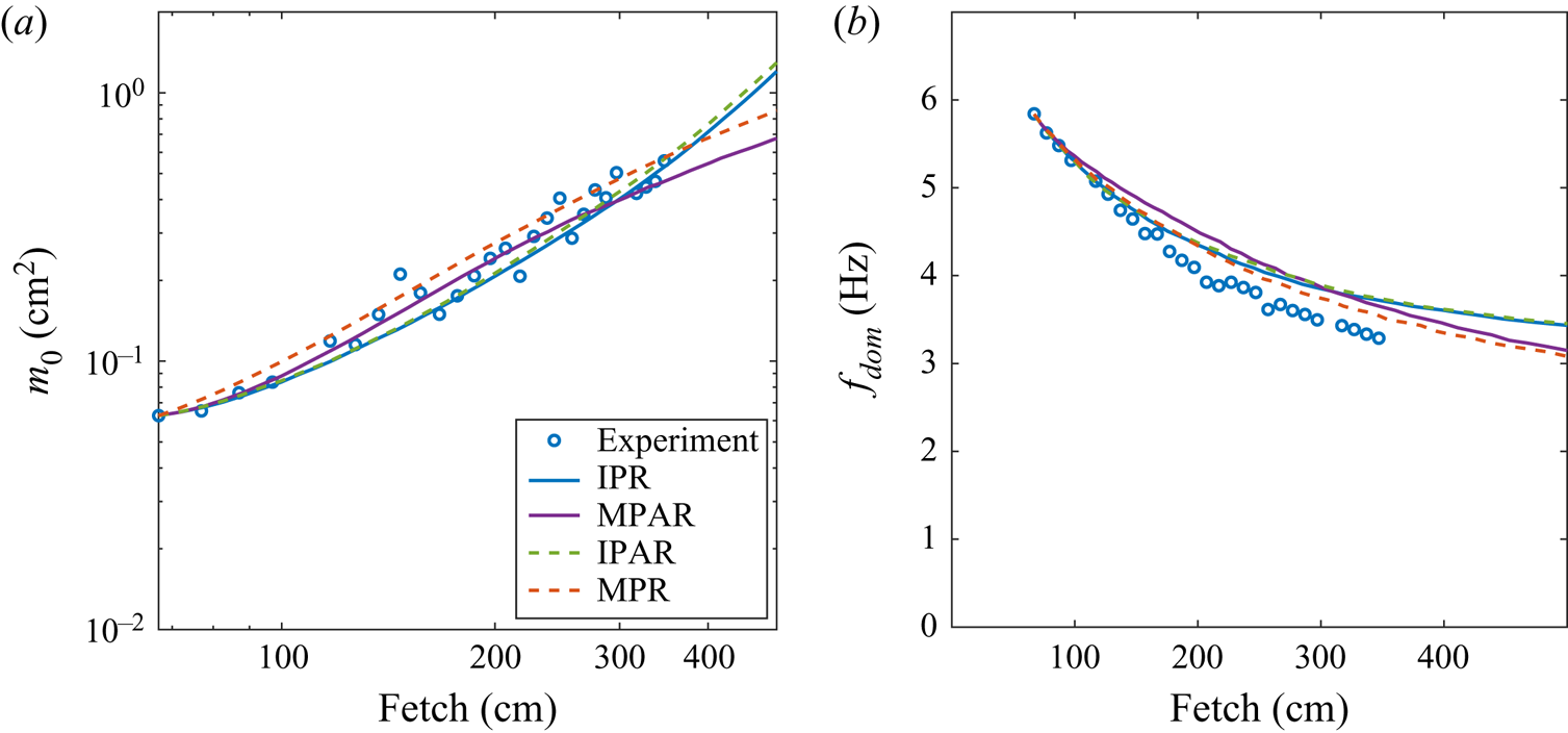
Comparison of simulations and experimental results for different randomization procedures, for wind velocity  $U = 8.5\ \textrm {m}\,\textrm {s}^{-1}$: $(a)$ variation of the wave energy with fetch, and $(b)$ variation of the dominant frequency.
The change of the effective viscosity affects not only the total wave energy but also the variation of the dominant frequency with fetch. This effect is studied in figure 3(b) where the values of  $a$ are adjusted to ensure wave energy growth as observed in experiments. The linear simulations show that, for very young waves, dissipation in the boundary layer below the air–water interface due to effective viscosity may play a significant role in the frequency downshifting with fetch. As expected, no change in $f_{dom}$ with fetch is obtained in the linear model solution when viscous dissipation is neglected. However, even for the lowest possible dissipation caused by the molecular viscosity of water, the adopted model predicts some modest (approximately 0.4 Hz) decrease in the dominant frequency. The frequency downshifting increases with increase in $\nu _{eff}$ up to approximately $\nu _{eff} = 0.08\ \textrm {cm}^{2}\,\textrm {s}^{-1}$. Increase of effective viscosity beyond $\nu _{eff} = 0.08\ \textrm {cm}^{2}\,\textrm {s}^{-1}$ practically does not affect the dominant frequency downshift of approximately 1 Hz along the simulation domain, well below the frequency downshifting by more than 2.5 Hz as observed in the experiments for $U = 8.5\ \textrm {m}\,\textrm {s}^{-1}$.
5. Experimental results versus numerical simulations
The solutions of the set of equations (3.7) with amplitude spectra measured at  $x_0 = 67\ \textrm {cm}$ used to determine the initial conditions for all wind velocities are now compared with the experimental results. For all wind velocities, the values of the two empirical coefficients, $a = 0.0235$ that determines the net wind input in (3.2) and $\nu _{eff} = 0.08\ \textrm {cm}^2\,\textrm {s}^{-1}$, were retained.
5.1. Various approaches to account for the random and three-dimensional nature of wind waves
As discussed in §§ 3.5 and 4, irregularity and directional spreading characterize wind waves in the laboratory as well as at larger scales in nature. They play a fundamental role in Reference PhillipsPhillips's (Reference Phillips1957) theory of wave generation by wind. The model equations (3.7), however, are quasi-deterministic and unidirectional. The results of different approaches to mimic in simulations the loss of spatial coherence of wind waves are now assessed by comparing the model predictions with experiments. The most straightforward way to represent the irregularity of wind waves at the initiation of simulations is by prescribing a random uniformly distributed phase to each mean amplitude in the spectrum in the initial conditions (see § 4). Monte Carlo simulations of multiple realizations of the spectrum with initial phase randomization (IPR) were therefore performed. Alternatively, the amplitudes of each frequency harmonic can also be randomized assuming a Gaussian distribution with standard deviation as obtained in experiments. The runs where both the initial phases and amplitudes were randomized are denoted as IPAR.
The IPR and IPAR simulations yield results that are in a reasonable agreement with experiments (see figure 4). Close similarity between the curves corresponding to IPR and IPAR simulations in figure 4(a,b) indicates that randomization of the initial amplitudes, in addition to randomization of the initial phase, does not affect the outcome notably. Within the domain of available experimental data, the wave energy in those simulations increases in agreement with the measurements. However, at larger fetches the increase of the energy with  $x$ becomes faster and deviates significantly from linear growth. The dominant frequency in those simulations exhibits significant downshifting that is quite close to that observed in the experiments (see figure 5b). At larger fetches, the rate of frequency downshifting with fetch decreases notably, unlike the trend in the dependence $f_{dom} (x)$ observed in the experiments.
Comparison of experimental results at  $U = 6.3\ \textrm {m}\,\textrm {s}^{-1}$ with linear and nonlinear model solutions for spatial evolution of: $(a)$ wave energy and $(b)$ dominant frequency.

IPR and IPAR runs simulate the irregularity of the initial conditions. However, each individual realization in the model computations remains fully deterministic and unidirectional so that the three-dimensional nature of wind waves is unaccounted for in those simulations. It is plausible to assume that the rapid loss of both spatial and temporal coherence of wind waves as discussed in § 3.5 is associated with the directional spreading.
In an attempt to account for limited spatial coherence using a unidirectional and essentially deterministic computational model, additional computations were performed where randomization was carried out in the course of integration at multiple locations. In the present simulations, randomization was performed at each station where the dominant frequency was adjusted, as specified in § 4.2. Again, two possible approaches were examined. First, multiple randomization of phases only (MPR) was applied, while the amplitudes of the spectral harmonics at each station were assigned fixed values corresponding to those computed in the integration procedure up to that point power-spectrum-averaged over all individual runs. The computations were then resumed with those new initial conditions along the segment with the length corresponding to the local dominant wavelength  $\lambda _{dom}(x)$. This selected spatial separation between successive randomization locations is in agreement with the available results on the spatial coherence of random wave fields as presented in § 3.5. In the last series of simulations, denoted by MPAR, both phases and amplitudes were repeatedly randomized at those stations in the course of integration. The effect of the length of the segment after which randomization was carried out was examined in additional runs with more frequent multiple randomizations at ${\rm \Delta} x =0.5\lambda _{dom}$. Those tests demonstrated that the simulation results are practically insensitive to the selection of ${\rm \Delta} x$.
There is a substantial similarity in the outcomes of different randomization procedures, and all adopted procedures yield results that do not differ significantly from the experiments. However, randomizations performed at multiple locations in the course of integration lead to a linear wave energy growth along the whole computational domain, in agreement with the results of Mitsuyasu & Honda (Reference Mitsuyasu and Honda1982). Randomization of amplitudes in addition to that of phases in the MPAR runs leads to somewhat slower energy growth with  $x$ as compared to phase randomizations only in MPR (see figure 4a). There is practically no effect of multiple amplitude randomizations on frequency downshifting, and the curves corresponding to MPR and MPAR in figure 4(b) are quite close.
It should be noted that the computational procedure (MPAR) that involves combined multiple amplitude and phase randomization requires larger ensembles of runs as compared to simulations (MPR) in which only the phases were randomized. In most cases, in order to obtain smooth curves representing the dependences  $m_0(x)$ and $f_{dom}(x)$, 100 independent realizations of the initial spectrum were sufficient in MPR simulations, whereas accounting for irregular amplitudes in the MPAR procedure required at least 400 realizations. Since, within the spatial domain that corresponds to the range of fetches where the measurements were carried out, both MPR and MPAR procedures yield results that agree well with measurements, the MPR approach is applied in what follows for comparison of the experimental and numerical results.
5.2. Effect of nonlinearity
The theoretical model presented above is now applied to assess the contribution of nonlinearity to the evolution of the wind waves with fetch. The spatial variations of the wave energy,  $m_0(x)$, and of the dominant frequency, $f_{dom}(x)$, obtained by solving the nonlinear model (3.7) with MPR are compared with the predictions of the linear model (4.2) in figure 5. Since randomization of phases does not affect the results of the linear model, initial amplitude randomization was applied to obtain an ensemble of realizations for a given initial spectrum. While the wave energy growth with fetch $x$ obtained in linear approximation is identical in all realizations, the individual spectra and thus the dominant frequency vary.
As expected, the linear model, while describing reasonably well the initial stages of the spatial evolution, yields explosive exponential growth of the wave energy with fetch, with wave amplitudes significantly exceeding the measured values (see figure 5a). The results of the nonlinear model are in good agreement with experiments; both are characterized by a close-to-linear growth of wave energy with fetch for  $x> 100\ \textrm {cm}$. As already demonstrated in figure 4(a), linear energy growth is obtained in the simulations when not only the nonlinearity, but also the wave field irregularity, is accounted for by applying the MPR procedure. The dominant frequency downshift is predicted by both linear and nonlinear models. The adopted version of the linear model, in which the spatial (but not the temporal) rates of change of wave amplitudes due to dissipation and net wind input vary with frequency, allows for frequency downshifting (see § 4). The frequency downshifting due to the contribution of linear mechanisms, while non-negligible, is significantly smaller than that observed in experiments. Incorporation of nonlinearity in the model increases the dominant frequency downshifting significantly, yielding results that are quite close to the experimentally measured values. As seen in figure 4(b), the wave field irregularity simulated by application of the multiple randomization procedure does not have a notable effect on $f_{dom}(x)$.
In order to assess the role of nonlinearity and wind input separately, the nonlinear model (3.7) was solved in the absence of dissipation in the surface boundary layer due to effective kinematic viscosity. Computations with  $\nu _{eff} = 0$ were performed by applying the MPR procedure. The resulting variations of the wave energy, dominant frequency and amplitude spectra with fetch are plotted in figure 6(a–c). To account for neglecting the dissipation term in (3.7), an appropriate adjustment of the net wind input coefficient $a$ was performed. This adjustment enables one to obtain reasonably good agreement between simulations and experiments in wave energy growth with fetch (see figure 6a). The results plotted in figure 6(b) demonstrate that, in the absence of effective viscosity, a certain downshift of the dominant wave frequency due to nonlinear interactions is still obtained. However, this downshift in figure 6(b) is significantly smaller than that measured experimentally. The computed amplitude spectra plotted in figure 6(c) suggest that, following the initial early development stage, the wave energy supplied by wind in the vicinity of the spectral peak is transferred by nonlinearity to both higher and lower frequencies. In analogy with hydrodynamic turbulence, these nonlinear energy transfers are often termed ‘direct’ and ‘inverse’ cascades, respectively (Zakharov & Filonenko Reference Zakharov and Filonenko1966; Zakharov & Zaslavsky Reference Zakharov and Zaslavsky1983; Annenkov & Shrira Reference Annenkov and Shrira2006). The energy transfer to lower frequencies results in spectral peak downshifting, whereas, in the absence of dissipation, the direct cascade causes accumulation of wave energy at high frequencies.
Nonlinear model solutions without effective kinematic viscosity,  $\nu _{eff} = 0$, for $U = 8.5\ \textrm {m}\,\textrm {s}^{-1}$. Variation with fetch of $(a)$ wave energy $m_0$, $(b)$ dominant frequency $f_{dom}$ and $(c)$ the computed amplitude spectra.

5.3. Spectral shapes
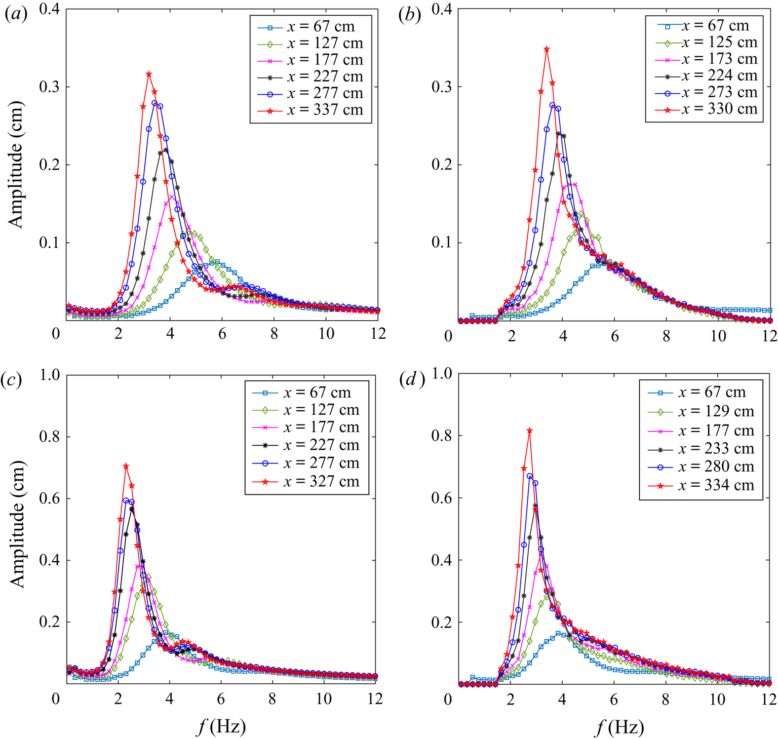
The evolution of the wave amplitude spectra with fetch in experiments and in simulations is presented in figure 7(a,b) and (c,d) for two wind velocities: a relatively weak wind with  $U = 8.5\ \textrm {m}\,\textrm {s}^{-1}$, and the strongest wind forcing applied in the present experiments, $U = 11.5\ \textrm {m}\,\textrm {s}^{-1}$, respectively. For each wind forcing condition, the initial spectra in simulations at fetch $x = 67\ \textrm {cm}$ are obviously identical to those measured in the experiments that defined the initial conditions in the simulations. The spectra obtained in simulations and in experiments are plotted at close locations. At both wind velocities, the evolution of the shape of the amplitude spectra in simulations is in good agreement with the experimental results. The frequency downshifting as well as the peak amplitude growth in simulations are qualitatively and to a large extent quantitatively similar to those obtained in the measurements. Note that the evolution of free waves only was studied in simulations; no attempt was made to compute the contribution of the bound waves around the second harmonic of the peak frequency, although those computations can be readily performed within the framework of the Zakharov equation (see Krasitskii Reference Krasitskii1994). The second-order bound waves clearly visible as secondary peaks in the measured spectra at larger fetches at higher wind velocity (figure 7c) contribute to the quantitative disagreement between the simulated and measured spectra away from the spectral peaks.
Evolution of wave amplitude spectra along the tank: comparison of ( $a$,
$a$, $c$) experimental results and ( $b$,
$b$, $d$) simulations at ( $a$,
$a$, $b$)
$b$)  $U = 6.3\ \textrm {m}\,\textrm {s}^{-1}$ and ( $c$,
$c$, $d$)
$d$)  $U = 11.5\ \textrm {m}\,\textrm {s}^{-1}$.
The variation with fetch of the dimensionless spectral width  $\epsilon$ defined by (3.5) is studied in figure 8 for the whole range of wind velocities $U$ employed. The experimental results are plotted in figure 8(a), while the model predictions are presented in figure 8(b). The dimensionless spectral width decreases from the initial value of approximately $\epsilon = 0.2$ to $\epsilon \approx 0.14$ for all wind velocities in experiments and in simulations. The decrease in $\epsilon$ in experiments is gradual and close to monotonic, while the model yields a dimensionless steepness that initially decreases faster, attains a minimum and then increases back. These differences between the curves representing the variation with fetch of the dimensionless spectral width $\epsilon$ in experiments and in simulations are much more pronounced at lower wind velocities, whereas for $U\geq 6.3\ \textrm {m}\,\textrm {s}^{-1}$ good quantitative and qualitative agreement is observed between figures 8(a) and 8(b) along the whole test section.
Evolution of the dimensionless spectral width  $\epsilon$ along the tank for various constant wind velocities $U$:
$U$:  $(a)$ experimental results and $(b)$ simulations.

5.4. Variation with fetch of wave field parameters
Variation with fetch of the measured total wave energy is compared in figure 9(a) with the simulation results for different wind velocities. For all wind forcing conditions, this figure demonstrates good agreement between the model and the experimental results, with the energy growth with fetch close to linear. At higher wind velocity, the model predictions at larger fetches overestimate the wave energy. This may be attributed to greater sensitivity to end effects of larger and longer waves approaching the far end of the test section. A similar effect at the far end of the test section was observed in Liberzon & Shemer (Reference Liberzon and Shemer2011).
Variation of  $(a)$ the total energy and $(b)$ dominant frequency $f_{dom}$ of free waves in the spectrum with fetch for different wind forcing conditions. Symbols are experimental results; and solid lines are model predictions.

The agreement between the variations with fetch of the dominant frequency,  $f_{dom}(x)$, in experiments and in model computations plotted for different wind velocities $U$ in figure 9(b) is satisfactory but less impressive than that obtained for wave energy growth in figure 9(a). The model gives a qualitatively correct downshifting of the dominant frequency with $x$; the decrease of $f_{dom}$ along the test section in simulations increases with the wind velocity $U$ as in the experiments. However, the rate of decrease in $f_{dom}(x)$ in simulations is somewhat smaller than that in the experiments. This discrepancy between experimental and numerical results is more prominent for lower wind velocities.
The spatial variations of the characteristic wave amplitude,  $m_0^{1/2}$, and of the dominant frequency, $f_{dom}$, are presented in figure 10 in a dimensionless form following Kitaigorodskii (Reference Kitaigorodskii1962) for all wind velocities $U$ employed in this study. Using $u_{\ast }$ as the characteristic velocity, the dimensionless parameters are defined as follows: the dimensionless fetch $\hat {x}=gx/u_{\ast }^2$, the characteristic wave amplitude $\hat {m}_0^{1/2}=m_0^{1/2}g/u_{\ast }^2$, and the dominant frequency $\hat {f}_{dom}=u_{\ast }f_{dom}/g$. It is customary to present the dependences of $\hat {m}_0^{1/2}$ and $\hat {f}_{dom}$ on the dimensionless fetch $\hat {x}$ as $\hat {m}_0^{1/2}=c_1\hat {x}^{b_1}$ and $\hat {f}_{dom}=c_2\hat {x}^{-b_2}$, respectively, where $b_1$, $c_1$ and $b_2$, $c_2$ are non-dimensional constants (Mitsuyasu Reference Mitsuyasu1968).
The variations of ( $a$,
$a$, $b$) the dimensionless amplitude $\hat {m}_0^{1/2}$ and ( $c$,
$c$, $d$) the dominant frequency $\hat {f}_{dom}$ with the dimensionless fetch $\hat {x}$ for different wind forcing conditions: ( $a$,
$a$, $c$) results of experiments and ( $b$,
$b$, $d$) results of simulations. The solid line in each panel denotes the linear fit to the data obtained for higher wind velocities only.

Figure 10 summarizes the main experimental and numerical results accumulated in this study. Comparison of figures 10(a,c) and 10(b,d) demonstrates that the suggested model adequately describes the variation of wave amplitudes and dominant frequencies with fetch for all wind velocities. The qualitative difference in behaviour of  $\hat {m}_0^{1/2}(\hat {x})$ and $\hat {f}_{dom}(\hat {x})$ at higher wind velocities as compared to lower velocities is clearly seen in figure 10 in the experimental as well as in the numerical results. For higher wind velocities, $U = 10.6\ \textrm {m}\,\textrm {s}^{-1}$ and $U = 11.5\ \textrm {m}\,\textrm {s}^{-1}$, both $\hat {m}_0^{1/2}(\hat {x}$) and $\hat {f}_{dom}(\hat {x})$ exhibit a linear dependence in log–log coordinates corresponding to power-law behaviour and collapse onto a single line, with very similar coefficients $b$ and $c$ in experiments and simulations. The values of the coefficients of the power law obtained in the present study are also close to those reported in laboratory experiments by Mitsuyasu (Reference Mitsuyasu1968) and Zavadsky, Liberzon & Shemer (Reference Zavadsky, Liberzon and Shemer2013). Moreover, they are comparable to those obtained by Kahma (Reference Kahma1981) and in additional field experiments summarized by Badulin et al. (Reference Badulin, Babanin, Zakharov and Resio2007). Note also that, in most studies, the value of the exponent $b_1$ is close to 0.5, indicating growth of the energy of gravity wind waves with fetch that is close to linear.
For lower wind velocities that correspond to larger dimensionless fetches  $\hat {x}$, the behaviour of $\hat {m}_0^{1/2}(\hat {x})$ and $\hat {f}_{dom}(\hat {x})$ deviates notably from a power law. A similar deviation from a power dependence at weaker wind forcing was also reported by Zavadsky et al. (Reference Zavadsky, Liberzon and Shemer2013). Note that, unlike for stronger wind forcing, for the lower values of $U$ waves in our experimental facility are quite short and affected by capillarity along a significant part of the test section; so that the relative contribution of gravity and surface tension varies in the course of wave propagation. Nevertheless, the shapes of the curves in both columns of figure 10 are indeed quite similar, with a reasonable quantitative agreement.
6. Discussion
The computational model suggested and verified experimentally in this study attempts to describe in a quantitatively accurate manner an extremely complex phenomenon of wind interaction with water surface. Even for the simplest case of constant wind velocity  $U$ studied here, many details of this interaction are still far from being fully understood. In spite of extensive theoretical and experimental efforts during recent decades, the relative importance of different mechanisms for energy and momentum transfer from wind to waves is not yet known even for the two-dimensional monochromatic waves that have been considered in most studies. While it is commonly agreed that wave breaking constitutes the major factor causing loss of wind-wave energy, the details of this process, which may differ significantly for wind waves of different wave age $c_p/u_{\ast }$, remain uncertain. Parameters such as the rate of energy loss and the spectral changes associated with a single breaking event are not yet documented well enough even for unidirectional regular waves in the absence of wind. The random and three-dimensional nature of wind waves and of their breaking, the role of droplet detachment due to wind, and additional possible mechanisms complicate the situation further and effectively prevent detailed quantitative description of wind-wave energy loss due to breaking.
It is often suggested that, while wind input and dissipation are of fundamental significance for the very existence of wind waves, their particular details are less important, and the dynamics of wind waves is mainly governed by nonlinear processes (Zakharov et al. Reference Zakharov, Badulin, Hwang and Caulliez2015). In the present study, both wind input and wave energy dissipation were introduced by simple phenomenological modelling. Based on the available experience as described in §§ 3.3 and 3.4, it is assumed that wind input as well as wave breaking are associated with high waves that may have short duration and emerge locally as a result of constructive interference of multiple energy-containing harmonics. The wind input and wave energy loss by breaking are therefore not localized in the Fourier frequency space, but rather distributed in the vicinity of the local dominant frequency. The adopted model for net wind input leans on Plant (Reference Plant1982) and Hwang & Sletten (Reference Hwang and Sletten2008) and lumps the effects of wind input and wave breaking into a single linear term in (3.7). A single empirical coefficient in this linear term was applied for all wind velocities.
An additional linear term is included in (3.7) to account for dissipation under the water surface as given by Lamb (Reference Lamb1932) for the molecular kinematic water viscosity  $\nu$, but taking a larger effective kinematic viscosity value $\nu _{eff}$. The role of this term is to eliminate accumulation of energy at high frequencies due to the nonlinear direct cascade to shorter waves as demonstrated in figure 6(c). A single empirical value of $\nu _{eff} = 0.08\ \textrm {cm}^{2}\,\textrm {s}^{-1} >\nu$ was selected to account for turbulence under wind waves at all wind velocities $U$. The simulation results presented in figure 7 demonstrate that even this simplest possible and very crude model is capable of a reasonably accurate prediction of the behaviour of the spatial spectral evolution of young gravity–capillary wind waves in our facility.
The numerical model employed in the present study (see § 3.6) is based on the spatial version of the Zakharov equation. Evolution of the complex amplitude of each frequency harmonic along the test section is computed starting from the initial value based on wave spectra measured in our facility in the matching experiments at a short fetch  $x_0 = 67\ \textrm {cm}$, as described in § 4.1. To account for wind-wave irregularity, Monte Carlo simulations were performed. However, the results of simulations demonstrate that the close-to-linear growth of the wave energy with fetch $x$ as observed in experiments can approximately be reproduced in simulations for a limited range of fetches only. At larger distances, the spatial rate of growth of the wave energy increases notably (see figure 4a). This close-to-exponential growth of wave energy in simulations based on randomization of the initial conditions only may be expected since, for each frequency harmonic, the wind input is modelled by a linear term, see (4.2), while the nonlinearity only redistributes the energy within the spectrum.
The wind input modelling adopted here originates from the theory by Miles (Reference Miles1957, Reference Miles1959), which is linear and deterministic, and thus predicts exponential growth in time. These features were retained in later developments of the theory – for more details, see Shemer (Reference Shemer2019). However, experiments on wind-wave growth under impulsive forcing by Zavadsky & Shemer (Reference Zavadsky and Shemer2017b) demonstrate that the exponential growth stage is extremely short, and is followed by stages with growth that is essentially linear in time. The behaviour observed in their study was in general agreement with the theory of wind-wave generation by Phillips (Reference Phillips1957), which is essentially stochastic and accounts for directional spreading. These observations, as well as extensive experimental evidence to the irregular nature of wind waves as discussed in § 3.5, prompted an attempt to enhance the irregularity in simulations and mimic the directional spreading by introducing repeated randomizations at multiple locations along the integration path. Multiple randomizations indeed result in an effectively linear growth of wave energy with fetch in the present simulations (see figures 4, 5 and 7).
The evolution of wave spectra with fetch is characterized not only by wave energy growth with fetch, but also by peak frequency downshifting (see figure 1). While the spatial variation of the wave energy in simulations can be directly affected by proper tuning of the coefficient  $a$ in (3.2), there is no straightforward way in the adopted model to control the dominant frequency downshifting. Frequency downshifting is often attributed mainly to wave nonlinearity; the present model allows one to examine this conjecture. For the very young wind waves studied here, the frequency dependence of the spatial growth rate coefficient $\delta _j$ defined by (4.2) makes possible certain frequency downshifting by purely linear effects, depending on the values of the two tunable coefficients in the model, $a$ and $\nu _{eff}$. Such downshifting was indeed obtained in the solutions of the linear model (see figure 5b). The amount of linearly obtained downshifting, however, is well below that observed in the experiments. As demonstrated in figure 3(b), increase of the effective viscosity beyond the adopted value does not contribute to an additional decrease with fetch of the dominant frequency. On the other hand, simulations performed when the viscous dissipation in the model was switched off, so that nonlinearity remained the main factor capable of causing frequency downshifting, also results in reduction of the dominant frequency, albeit much less pronounced than in the experiments. Only the combination of nonlinearity and dissipation in the model leads to frequency downshifting that is quite close to the measured values. It is worth mentioning that the irregularity introduced into the model by repeated randomization of the spectra, while being essential for proper description of wave energy variation with fetch, becomes important for adequate presentation of the frequency downshifting only at larger fetches (see figure 4b).
The quality of the model predictions decreases somewhat with decreasing wind velocity  $U$, as can be seen in figure 9. The scaling exponents as discussed in relation to figure 10 pertain to pure gravity waves, while at weaker wind forcing shorter gravity–capillary wind waves are observed in the present experiments along a significant part of the test section. Moreover, while the effect of capillarity is taken into account in computation of the nonlinear interaction coefficients in (3.7), short gravity–capillary waves are also affected by induced surface currents (Liberzon & Shemer Reference Liberzon and Shemer2011; Zavadsky & Shemer Reference Zavadsky and Shemer2017a). Those effects, however, cease to be relevant for larger fetches and longer waves and were not considered in the present model.
Presentation of the characteristic integral properties of the wind wave field in dimensionless scaled form in figure 10 demonstrates that the spatial evolution patterns under steady wind forcing observed in the present experiments and successfully reproduced by the suggested model are in a reasonable quantitative agreement with results obtained in a large wind-wave tank by Mitsuyasu & Honda (Reference Mitsuyasu and Honda1982), as well with numerous additional experiments at much larger scales surveyed in Badulin et al. (Reference Badulin, Babanin, Zakharov and Resio2007); an updated list of experiments on wind-wave growth is available in Zakharov et al. (Reference Zakharov, Badulin, Geogjaev and Pushkarev2019).
7. Conclusions
In spite of impressive progress attained over the years in the prediction of ocean waves using theoretical and numerical models, many questions regarding wind–wave interaction remain unresolved. Ocean-scale models are not directly applicable for description of wind waves in a small laboratory facility that evolve fast with fetch. Careful experiments in wind-wave tanks under controlled conditions provide characterization of waves with accuracy and resolution that is unattainable in field measurements. Such experiments are combined in the present study with nonlinear modelling that is adjusted to waves evolving under steady wind forcing along the test section of a moderately sized wind-wave facility. The model allows one to perform a detailed comparison of the numerical simulations with measurements of wind-wave field evolution with fetch, which were performed for a range of wind velocities  $U$. To the best of our knowledge, no such detailed comparison of simulations with experimental results has been attempted so far. The suggested model thus serves as a tool for studying the relative importance of different mechanisms contributing to the evolution of young wind waves.
The model is based on a unidirectional spatial version of the Zakharov equation; wind input and dissipation are accounted for by additional linear terms. The quasi-deterministic model describes the spatial evolution of each frequency harmonic. It is assumed that both wind input and dissipation due to breaking are not localized in the frequency space, but rather spread over the whole spectrum; they affect primarily the vicinity of the local dominant frequency. In addition, simple modelling of dissipation of very short waves in the boundary layer under the air–water interface due to effective turbulent viscosity is included.
The present model contains only two adjustable empirical parameters: the fixed values of those parameters were used for simulations of the wave field evolution along the test section at all wind forcing conditions. Consistently good agreement was obtained between the experimental and the numerical results.
The simulations demonstrate that a moderate dominant frequency downshifting can be obtained in the framework of the linear approach. An attempt to neglect viscous dissipation of short waves while retaining nonlinearity yielded a frequency downshift well below the experimentally observed values. The combination of all terms on the right-hand side of the governing equation (3.7) is required to obtain in the simulations a dominant frequency downshifting that is close to the experimentally obtained values.
Irregularity has a pronounced role in the spatial evolution of wind waves. In the present study, the quasi-deterministic model approach was amended by Monte Carlo simulations with multiple realizations of the initial spectrum with random phases and/or amplitudes. Moreover, it is demonstrated that rapid loss of coherence and the directional spreading of waves as observed in experiments can effectively be modelled within the unidirectional model by carrying out multiple randomization procedures of the computed spectra at numerous locations in the course of integration.
The model thus combines Miles’ linear approach (Miles Reference Miles1957, Reference Miles1959) to describe the temporal exponential growth of individual frequency harmonics with Phillips’ theory (Phillips Reference Phillips1957) that emphasizes the randomness and directional spreading of wind waves. The resulting model indeed yields a reasonably good quantitative agreement with the results of extensive experiments on the evolution of a young wind-wave field with fetch.
An effort was made to offer a model as simple as possible. Nevertheless, the performance of the model demonstrates that it is not oversimplified and describes adequately the major processes in the spatial evolution of wind waves in a laboratory tank.
Some mechanisms governing the evolution of the wave field along the test section discussed in the present study are apparently limited to the very young and short waves studied here. Nevertheless, it is important to stress that the quantitative similarity between relations describing the spatial variation of the integral wave parameters with fetch in the dimensionless scaled form obtained in the present study with those generally accepted for wind-wave evolution at much larger scales suggests that the significance of the present results may extend beyond the size of the facility.
Acknowledgements
Support of this research by the Israel Science Foundation (grants #306/15 and #508/19) is gratefully acknowledged. The authors thank Dr. A. Khait and G. Rosenman for help and advice.
Declaration of interests
The authors report no conflict of interest.


 Open access

