


1. Introduction
The minimization of pressure losses within conduits is of great interest as otherwise there is likely to be an unnecessary energy cost incurred to maintain the movement of fluid. Such losses stem from one of two main origins: they can be created by the interaction of pressure with the solid walls thereby leading to interaction drag (Mohammadi & Floryan Reference Mohammadi and Floryan2012) or arise from the friction between the fluid and the boundaries. Mechanisms that create frictional drag are reasonably well understood but possible strategies to control and reduce this drag are not so advanced. The results presented in this paper provide some general guidance as to how heating patterns might be used to reduce frictional drag. This is accomplished by encouraging the formation of a net buoyancy force, thereby providing propulsion augmentation in vertical conduits. At face value it might seem that by simply imposing a strong thermal gradient on the slot one could reduce the density of fluid and hence promote the buoyancy effects. Unfortunately, this elementary technique is rarely helpful because the magnitude of the permitted temperature differences is restricted by potential changes in the thermophysical properties of the fluid; this limitation is especially pertinent when the conduit is long. An alternative approach is proposed in this paper where the use of distributed heating patterns with zero mean value is suggested; this eliminates the need for large temperature differences. The resulting thermal field is now known as structured convection (Hossain & Floryan Reference Hossain and Floryan2013) – a term that is used to reflect the fact that its well-defined topology is controlled by the underlying heating pattern. This convection represents a forced system response which contrasts with the perhaps more familiar Rayleigh–Bénard convection that arises as a bifurcation from the pure conduction state. We point out that there is a well-developed and extensive literature that discusses convection driven by horizontal temperature gradients (Hughes & Griffiths Reference Hughes and Griffiths2008) but this cannot simply be extrapolated to vertical conduits.
Numerous studies of structured convection in horizontal channels have demonstrated conclusively the clear potential for using carefully chosen heating patterns to limit pressure losses (Hossain, Floryan & Floryan Reference Hossain, Floryan and Floryan2012; Floryan & Floryan Reference Floryan and Floryan2015; Hossain & Floryan Reference Hossain and Floryan2016; Inasawa, Taneda & Floryan Reference Inasawa, Taneda and Floryan2019). A similar effect can be achieved when looking at the driving force required to maintain the relative movement of parallel plates (Floryan, Shadman & Hossain Reference Floryan, Shadman and Hossain2018). This reduction can be achieved whether the heating is applied to the upper or lower wall, or both (Hossain & Floryan Reference Hossain and Floryan2014, Reference Hossain and Floryan2015a) and results from the formation of flow separation structures that we shall refer to as `bubbles’. These bubbles underpin the operation of three separate effects. First, they reduce the direct contact between the stream and the sidewalls, thus reducing shear; second, the fluid rotates inside the bubbles owing to the heating-induced density gradients and so provides a supplementary propulsion force; and, lastly, the presence of the bubbles restricts the effective flow cross-sectional area which is known to contribute to enhanced pressure losses. The pressure-gradient-reducing effect disappears for excessively fast flows which tend to wash away the separation bubbles. A careful choice of parameter combinations can eliminate the need for a mean pressure gradient to drive the prescribed flow rate owing to heating-induced self-pumping.
The use of patterned heating in horizontal slots leads to interesting theoretical questions regarding the properties of structured convection. This convection commences as steady rolls with a spatial pattern dictated by the heating distribution. An increase in the intensity of heating leads to the formation of secondary states through an instability process that arises owing to a competition between the spatial parametric resonance and the Rayleigh–Bénard mechanism (Bénard Reference Bénard1900; Rayleigh Reference Rayleigh1916; Hossain & Floryan Reference Hossain and Floryan2013, Reference Hossain and Floryan2022). The details of this transition are sensitive to the fluid Prandtl number Pr. Additional complications can arise if the bounding walls are not flat but instead are corrugated as this leads to an interplay between the heating and topography patterns and the activation of this interaction effect (Floryan & Inasawa Reference Floryan and Inasawa2021) leads to the onset of thermal streaming (Abtahi & Floryan Reference Abtahi and Floryan2017b, Reference Abtahi and Floryan2018; Inasawa, Hara & Floryan Reference Inasawa, Hara and Floryan2021). Topography patterns can create their own convection even when the walls are isothermal; this convection is an example of a forced system response (Abtahi & Floryan Reference Abtahi and Floryan2017a). The combination of heating and groove patterns can lead to a reduction in pressure losses greater than that achievable by pure heating alone (Hossain & Floryan Reference Hossain and Floryan2020). The addition of forced convection can change the nature of the secondary states from stationary rolls to travelling waves (Hossain & Floryan Reference Hossain and Floryan2015b). It is unclear how this system response might change should the channel be orientated vertically. The limited results concerning natural convection in vertical and oblique channels suggest that a net buoyancy force can be generated even by periodic heating with zero mean and this gives rise to a propulsive force (Floryan, Haq & Panday Reference Floryan, Haq and Panday2022b; Floryan et al. Reference Floryan, Wang, Panday and Bassom2022c).
Heating-modified flows in vertical channels are of importance in various aspects of architectural design as they can affect the performance of heating, ventilation and air conditioning systems. Passive ventilation is achieved through the so-called stack effect, whereby a density difference drives the heated air in the upward direction, thereby drawing in cool air at the base of a structure (Linden Reference Linden1999; Wong & Heryanto Reference Wong and Heryanto2004; Mortensen, Walker & Sherman Reference Mortensen, Walker and Sherman2011; Nagler Reference Nagler2021). Conversely, in a reverse stack effect hot air is drawn down into a cooler environment. Such systems have performance limitations in terms of the maximum possible flow rate that can be achieved but this can be addressed by adding fans; this has the effect introducing a mean pressure gradient. An appreciation of the properties of flow in vertical channels is also helpful in the design of fire prevention measures in which effective control of the intensification and spreading of combustion is of utmost importance (Song et al. Reference Song, Huang, Kuenzer, Zhu, Jiang, Pan and Zhong2020). Upright fault lines are found in thermal recovery processes (Tournier, Gethon & Rabinowicz Reference Tournier, Gethon and Rabinowicz2000) and in hydraulic fracturing for gas recovery (Gandossi &Von Estorff Reference Gandossi and Von Estorff2015) with the relevant flows characterized by very small Reynolds numbers. The introduction of pressure gradients can also be used for enhancement of cooling by the chimney effect (Putnam Reference Putnam1882), which has been found to have contemporary applications in the passive cooling of electronic components (Naylor, Floryan & Tarasuk Reference Naylor, Floryan and Tarasuk1991; Straatman, Tarasuk & Floryan Reference Straatman, Tarasuk and Floryan1993; Straatman et al. Reference Straatman, Naylor, Tarasuk and Floryan1994; Novak & Floryan Reference Novak and Floryan1995; Shahin & Floryan Reference Shahin and Floryan1999; Andreozzi, Buonomo & Manca Reference Andreozzi, Buonomo and Manca2005; Mehiris et al. Reference Mehiris, Ameziani, Rahli, Bouhadef and Bennacer2017) as well as in the design of passively cooled nuclear reactors (Weil Reference Weil2012). The strength of the chimney effect can be significantly enhanced by using it in conjugation with an externally imposed pressure gradient. We remark that the intriguing concept of a horizontal chimney effect that relies on pattern interaction has been recently proposed (Floryan et al. Reference Floryan, Baayoun, Panday and Bassom2022a).
It is this plethora of practical applications that motivates the work described below. Here, we focus on the analysis of pressure-gradient-driven flows in vertical channels exposed to patterned heating. It is important to emphasize that our concern is exclusively with laminar flow and the thermal modulation of turbulent flows is outside the scope of our interest. Our starting point is provided by recent study of natural convection in smooth inclined slots exposed to a patterned heating (Floryan et al. Reference Floryan, Haq and Panday2022b) which predicts the formation of a net buoyancy force even for purely periodic heating patterns. A study of natural convection in a vertical grooved slot shows the importance of the pattern interaction effect and thermal streaming in such configurations (Floryan et al. Reference Floryan, Wang, Panday and Bassom2022c). In the current work we aim to determine how patterned heating might be used to reduce pressure losses. It is important to emphasize that we confine ourselves to the situation in which the two sides of the vertical channel have equal mean temperatures upon which are superimposed the patterned profiles. Moreover, we restrict ourselves to a study of Boussinesq fluids. In view of the large number of parameters present in the problem, the extension to a non-Boussinesq fluid (Paolucci Reference Paolucci1982; Frőhlich, Laure & Peyret Reference Frőhlich, Laure and Peyret1992), although perfectly possible in theory, would likely lead to a rather opaque and confusing picture. Here, the focus on the role played by the patterning.
The remainder of the paper is organized as follows. In § 2, we introduce our model, which consists of a vertical channel that contains a fluid moving upward together with heating patterns that are applied to the walls. To appreciate some of the properties of the flows we perform several computations that are described in §§ 3 and 4. In the first of these we examine the case when only one wall of the conduit is heated and then proceed in § 4 to extend our calculations to allow the heating to be applied to both walls. It is shown that the relative positions of the two heating profiles can have a dramatic effect on the size of the system response. We complement these numerical results with a closer examination of two cases that are amenable to theoretical analysis; in Appendix A we develop the solution structure generated by long-wavelength thermal modulation while the short-wavelength limit is discussed in Appendix B. We round off the paper with a few final remarks and discussion in § 5.
2. Problem formulation
Consider steady two-dimensional pressure-gradient-driven flow of a Boussinesq fluid contained in a vertical isothermal channel formed by two smooth parallel walls unbounded in the  $x$-direction. The sides of the channel are separated by a distance $2h$ and the gravity vector is supposed to act in the negative x-direction, as shown in figure 1. We scale distances on the half-channel width h (so the edges are located at $y ={\pm} 1$), fluid velocities on the maximum streamwise velocity ${u_{max}}$ and the pressure on $\rho u_{max}^2$, where $\rho $ denotes the density of the fluid. Then, in the absence of heating, we have the standard forms of the velocity ${\boldsymbol{v}_0} = ({u_0},{v_0})$ and pressure ${p_0}$ fields, together with the streamfunction ${\varPsi _0}$ and the flow rate ${Q_0}$ given by
 \begin{align}{\boldsymbol{v}_0}(x,y) = (1 - {y^2},0),\quad {p_0}(x,y) ={-} 2x/Re,\quad {\varPsi _0} = y - {\textstyle{1 \over 3}}{y^3} + {\textstyle{2 \over 3}},\quad {Q_0} = {\textstyle{4 \over 3}};\end{align}
here, the Reynolds number has been defined by  $Re = {u_{max}}h/\nu $, where $\nu $ is the kinematic viscosity.

Figure 1. A schematic of the flow system.
We now apply sinusoidal heating to both walls which means that their (dimensionless) temperatures are
 \begin{gather}y ={-} 1:{\theta _R}(x) = {\textstyle{1 \over 2}}R{a_{p,R}}\cos (\alpha x),\end{gather}
 \begin{gather}y ={+} 1:{\theta _L}(x) = {\textstyle{1 \over 2}}R{a_{p,L}} \cos (\alpha x + \varOmega );\end{gather}
 where here, and in what follows, we use the subscripts R and L to describe the properties relating to the right and left walls, respectively. If T denotes the absolute temperature, then we base the relative temperature  $\theta $ on the difference $T - {T_W}$, where ${T_W}$ is the mean temperature of the walls, and scale it using $\kappa \nu /(g\varGamma {h^3})$ as the temperature scale; here, g is the gravitational acceleration, $\varGamma $ denotes the thermal expansion coefficient and $\kappa$ is the thermal diffusivity. The intensities of the heating of the walls are described by the two Rayleigh numbers $R{a_{p,R}} = g\varGamma {h^3}{T_{p,R}}/(\kappa \nu )$ and $R{a_{p,L}} = g\varGamma {h^3}{T_{p,L}}/(\kappa \nu )$; here, ${T_{p,L}}$ and ${T_{p,R}}$ are the differences between the maximum and minimum of the left and right periodic temperature components, respectively. We point out that the two thermal profiles (2.2) are perfectly tuned in as much that they are characterized by the same wavenumber $\alpha$ although the two patterns incorporate a phase offset $\varOmega $.
Convection in the slot is governed by the scaled continuity, Navier–Stokes and energy equations that can be written as
 \begin{gather}u\frac{{\partial u}}{{\partial x}} + v\frac{{\partial u}}{{\partial y}} ={-} \frac{{\partial p}}{{\partial x}} + {\nabla ^2}u + P{r^{ - 1}} \theta ,\quad \frac{{\partial u}}{{\partial x}} + \frac{{\partial v}}{{\partial y}} = 0,\end{gather}
 \begin{gather}u\frac{{\partial v}}{{\partial x}} + v\frac{{\partial v}}{{\partial y}} ={-} \frac{{\partial p}}{{\partial y}} + {\nabla ^2}v,\quad u\frac{{\partial \theta }}{{\partial x}} + v\frac{{\partial \theta }}{{\partial y}} = P{r^{ - 1}}{\nabla ^2}\theta ,\end{gather}
where  $(u,v)$ are the velocity components in the (x, y) directions scaled on ${U_v} = \nu /h$, p is the pressure scaled with $\rho U_\nu ^2$ and $Pr = \nu /\kappa $ is the Prandtl number. The relevant boundary conditions take the forms
 \begin{equation}u( - 1) = u(1) = 0,\quad v( - 1) = v(1) = 0,\quad \theta ( - 1) = {\theta _L}(x),\quad \theta (1) = {\theta _U}(x),\end{equation}
where the functions  ${\theta _L}(x)$ and ${\theta _U}(x)$ are as defined in (2.2) and the flow fields can be decomposed as
 \begin{gather}u(x,y) = Re {u_0}(y) + {u_1}(x,y),\quad v(x,y) = {v_1}(x,y), \end{gather}
 \begin{gather}p(x,y) = R{e^2}{p_0}(x) + Bx + {p_1}(x,y),\quad \psi (x,y) = Re {\psi _0}(y) + {\psi _1}(x,y),\end{gather}
where the subscript 1 refers to modification to the reference flow (2.1) induced by the heating and B denotes the pressure-gradient correction. We are interested in determining whether the imposition of wall heating can lead to a reduction in the pressure gradient required to maintain the specified flow rate. Accordingly, we impose the mass flow rate constraint in the form
 \begin{equation}Q(x){|_{mean}} \equiv {\lambda ^{ - 1}}\int_{{x_0}}^{{x_0} + \lambda } {\int_{ - 1}^1 {u(x,y)\,\textrm{d}y\,\textrm{d}x} } = \frac{4}{3}Re,\end{equation}
where  $\lambda $ is the wavelength of the heating and Q is scaled using ${U_v}$. We seek information concerning the mean pressure gradient, i.e.
 \begin{equation}{\left. {\frac{{\partial p}}{{\partial x}}} \right|_{mean}} \equiv {\lambda ^{ - 1}}\int_{{x_0}}^{{x_0} + \lambda } {\frac{{\partial p}}{{\partial x}}\,\textrm{d}x} ={-} 2Re + B,\end{equation}
and remark that positive values of B signify a reduction in the pressure losses.
The system (2.2)–(2.6) was solved by expressing the velocity components using a streamfunction  $\psi $ defined in the usual manner, i.e. $u = \partial \psi /\partial y$, $v ={-} \partial \psi /\partial x$, eliminating pressure and then using Fourier expansions in the x-direction together with Chebyshev expansions in the y-direction. An extensive discussion of the algorithm and the benchmarking of its accuracy have been described elsewhere (Hossain et al. Reference Hossain, Floryan and Floryan2012) and the reader is referred to that paper for further details. The pressure field was normalized by bringing the mean value of its periodic component to zero while the mean Nusselt number $N{u_{av}}$ was evaluated using
 \begin{equation}N{u_{av}} ={-} {\lambda ^{ - 1}}\int_{{x_0}}^{{x_0} + \lambda } {{{\left. {\frac{{\partial \theta }}{{\partial y}}} \right|}_{y ={-} 1}}\,\textrm{d}x} .\end{equation}
With this definition, positive values of  $N{u_{av}}$ mean that the right wall losing energy. We remark that the shear forces acting on the fluid at the right and left walls are given by
 \begin{equation}{F_R} ={-} {\lambda ^{ - 1}}\int_0^\lambda {{{\left. {\frac{{\partial u}}{{\partial y}}} \right|}_{y ={-} 1}}\,\textrm{d}x} ,\quad {F_L} = {\lambda ^{ - 1}}\int_0^\lambda {{{\left. {\frac{{\partial u}}{{\partial y}}} \right|}_{y ={+} 1}}\,\textrm{d}x} ,\end{equation}
respectively, while the total (buoyancy) body force per unit length is given by
 \begin{equation}{F_b} = {\lambda ^{ - 1}}P{r^{ - 1}}\int_{ - 1}^1 {\int_0^\lambda {\theta \,\textrm{d}x\,\textrm{d}y} } .\end{equation}
3. Heating with an arbitrary wavenumber: one-wall heating
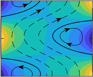
We commence our investigation into the problem by first looking at the case when we restrict the heating to just the right-hand wall  $(R{a_{p,L}} = 0)$; some typical flow patterns are displayed in figure 2. The flow topology for pure natural convection (when $Re = 0$) consists of a family of counter-rotating rolls (figure 2a). As the Reynolds number increases the flow pattern can undergo substantial modification. When $Re = 1$ we have a flow field that consists of convection-driven rolls combined with a stream tube that meanders between them and which carries fluid in the positive x-direction (see figure 2b). The net upward flow breaks various symmetries present in the natural convection and generates a mean buoyancy force as well as changing the shear forces that act on the two walls. A further increase to $Re = 5$ strengthens the stream tube and shrinks the size of the rolls, which can now be regarded as separation bubbles – the bubbles adjacent to the heated wall are appreciably larger (figure 2c). As $Re$ grows yet further this general process continues with the bubbles on the left wall becoming quite small when $Re = 10$ (figure 2d); they have completely disappeared by the stage $Re = 15$ (figure 2e). In contrast, the bubbles at the right wall persist irrespective of the value of $Re$ and the overall flow becomes essentially rectilinear when $Re = 100$ (figure 2f).

Figure 2. The flow and the temperature fields for one-wall heating with the parameter choices  $R{a_{p,R}} = 400$, $Pr = 0.71$ and $\alpha = 0.6$. In the sequence of plots the Reynolds number $Re$ is increased from $0$ to $100$. In (a) $Re = 0$, (b) $1$, (c) $5$, (d) $10$, (e) $15$ and (f) $100$. In all the plots the temperature has been normalized with its maximum ${\theta _{max}}$.
Heating-induced rolls tend to decrease the direct contact between the stream and the walls, thereby reducing the frictional resistance. The existence of separation bubbles diminishes the effective flow cross-sectional area, and this typically leads to an increase of pressure losses. The rotational motion of fluid within the bubbles themselves is partially driven by the buoyancy force associated with density variations – this effect provides some propulsion which reduces the pressure drop required to maintain a prescribed flow rate. The mean buoyancy force arises because the net fluid movement destroys symmetries which are present in pure natural convection and whether this force leads to either negative or positive propulsion depends on the flow conditions. The likely cumulative effect is difficult to predict without a careful and detailed analysis.
Figure 3 focuses on the profiles of various forces generated by the heating; in particular, the mean buoyancy force  ${F_b}$ as defined in (2.10) and the forces ${F_R}$ and ${F_L}$ (2.9) that act on the right and left walls, respectively. If the values taken by these latter two quantities for the case of an isothermal channel are denoted ${F_S}$ (note that the isothermal shears on the left and right walls are the same) then it is helpful to examine the differences $\mathrm{\Delta }{F_R} = {F_R} - {F_S}$ and $\mathrm{\Delta }{F_L} = {F_L} - {F_S}$, the sum $\mathrm{\Delta }{F_R} + \mathrm{\Delta }{F_L}$ together with the pressure-gradient correction B. The data displayed in figure 3(a) demonstrate the somewhat intricate role played by ${F_b}$ for the flow conditions illustrated here. We observe that ${F_b} = 0$ when $Re = 0$; it then rapidly increases with $Re$ until $Re \approx 5$, which suggests that this force is propelling the fluid. Once Re exceeds approximately 5, ${F_b}$ decreases and changes sign when $Re \approx 10$; now this buoyancy force opposes the fluid movement. Finally, it reaches a minimum value at $Re \approx 30$ before beginning to grow and becoming positive once more at $Re \approx 60$. The magnitude of the viscous force on the right wall decreases with its maximum value occurring when $Re \approx 10$. Heating always seems to increase the magnitude of the viscous force at the left wall, at least whenever the separation bubbles are present, but the sum of the two wall forces suggests that the overall viscous force is reduced. The pressure-gradient correction correlates well with variations of the mean buoyancy force and the total viscous force for the conditions used in figure 3(a). The shear stresses at the right wall increase near the hot spots and decrease near the cold spots, as illustrated in figure 3(b), with the cumulative effect shown in figure 3(a). The qualitative distribution of these stresses along the channel does not change much with $Re$ while the amplitude of their variations decreases as the separation bubbles are reduced and are eventually washed out. Shear stresses at the left wall increase opposite to the hot spots and decrease opposite to the cold spots, as illustrated in figure 3(c). Their magnitudes decrease much faster with $Re$ than those at the right wall.

Figure 3. (a) The forms of the buoyancy force  ${F_b}$, the viscous forces differences $\mathrm{\Delta }{F_R} = {F_R} - {F_S}$ and $\mathrm{\Delta }{F_L} = {F_L} - {F_S}$ at the two walls, the sum $\mathrm{\Delta }{F_R} + \mathrm{\Delta }{F_L}$ and the pressure-gradient correction B as functions of $Re$. Other parameter values are fixed at values $R{a_{p,R}} = 400,\, Pr = 0.71,\alpha = 0.6$. (b) The distribution of the viscous stress difference $\mathrm{\Delta }{\sigma _R} = {\sigma _{xv,R}} - {\sigma _{xv,S}}$ at the right wall and (c) the stress difference $\mathrm{\Delta }{\sigma _L} = {\sigma _{xv,L}} - {\sigma _{xv,S}}$ at the left wall where ${\sigma _{xv,S}}$ denotes the shear stress in an isothermal channel. In plots (b) and (c) five Reynolds numbers are used: $Re = 0$ (red lines), $1$ (green), $10$ (cyan), $25$ (purple), $100$ (black).
3.1. The role of the Prandtl number
The key role played by the mean buoyancy force raises the issue as to the importance of the Prandtl number. Asymptotic analysis presented later in the paper suggests that long-wavelength heating always reduces the pressure losses, but a similar reduction can be achieved in the short-wavelength limit only if Pr is sufficiently large. The conditions marking the transition between a reduction to an enhancement of pressure losses, together with the size of the pressure losses themselves, are illustrated in figure 4 – to gauge the effectiveness of heating the reader is reminded that when  $B = 2Re$ the pressure loss is zero. A plot of the mean buoyancy force as displayed in figure 5(a), which corresponds to the conditions used in figure 4(a), shows that this buoyancy force behaves in a similar fashion to the variations in the pressure-gradient correction. The shear at the right wall (see figure 5b) appears to be significantly reduced while that at the left wall generally increases, except when $\alpha $ and $Pr$ are large. The reduction in the total shear force as displayed in figure 5(d) correlates well with both the formation of the mean buoyancy force and the reduction in the pressure gradient. An increase in $Pr$ tends to strengthen the convection which in turn leads to an increase in the mean buoyancy force. When $Pr$ is very large, the buoyancy effects are confined to a boundary layer adjacent to the heated wall and reduces the mean buoyancy force as a smaller portion of the flow field is exposed to temperature variations. The buoyancy force also seems to decrease in the long-wavelength limit $\alpha \to 0$ as the magnitude of the temperature gradient decreases. A reduction in the buoyancy force is also noted in the short-wavelength structure $\alpha \to \infty $ ; now the temperature gradient becomes concentrated within a thin boundary layer adjacent to the heated wall. Changes in the viscous forces occur owing to modifications to the flow pattern and this leads to a pressure-gradient reduction similar in size to that which can be attributed to the buoyancy force.

Figure 4. The form of the pressure-gradient correction  $B/Re$ as a function of $\alpha $ and $Pr$ when $R{a_{p,R}} = 300$ for two values of the Reynolds number; (a) $Re = 1$ and (b) $Re = 10$. The region of parameter space shaded grey identifies those conditions that correspond to a reduction in the pressure losses.

Figure 5. The form of (a) the buoyancy force  ${F_b}$, (b) the force difference $\mathrm{\Delta }{F_R} = {F_R} - {F_{R,S}}$, (c) the force difference $\mathrm{\Delta }{F_L} = {F_L} - {F_{L,S}}$ and (d) the sum $\mathrm{\Delta }{F_R} + \mathrm{\Delta }{F_L}$ as functions of $\alpha $ and $Pr.$ The Rayleigh number $R{a_{p,R}} = 300$ and the Reynolds number $Re = 1$. The region of parameter space shaded grey identifies those conditions that correspond to a reduction in the losses.
To probe more deeply the properties of the flow structure we focused on the two values of the Prandtl number,  $Pr = 0.71$ and 7; these were chosen as they are the values appropriate to air and water, respectively. The form of $B(\alpha )$ is illustrated in figure 6. It is evident that the largest absolute value of B occurs at some $\alpha = O(1)$ value and falls off towards zero as $\alpha \to 0$ and $\alpha \to \infty $ – these limits are analysed in the appendices. It is also noted that the sign of B changes at some $\alpha = O(1)$ whose value(s) is a function of the other parameters in the problem. For example, when $Pr = 0.71$ there appear to be two ranges of $\alpha $; for relatively small values there is a reduction in the pressure losses but at larger values there is a significant increase of these losses. It seems that the critical value at which the transition between these contrasting behaviours occurs between these zones moves towards smaller α values as $R{a_{p,\, R}}$ increases, see figure 6(a,c). The details of this response are only slightly affected by an increase in the Reynolds number from $Re = 1$ to $Re = 10$. The situation changes somewhat at the higher Prandtl number $Pr = 7$. Now a reduction in the pressure losses is observed for all values $\alpha $ unless $R{a_{p,\, R}}$ becomes particularly large – this is illustrated in figure 5(b) for $R{a_{p,\, R}} = 1000$ for which, over a small range of $\alpha $, increasing losses are noted. An increase in $Re$ from $Re = 1$ to $Re = 10$ sees the elimination of the short range. In summary we conclude that an increase in $R{a_{p,\, R}}$ does not inevitably lead to a larger reduction in the pressure losses, and an increase in $Re$ does not necessarily result in a modification of the pressure losses.

Figure 6. The variation in the pressure-gradient correction quantity  $|B/Re|$ as a function of the heating wavenumber $\alpha $. Dashed lines denote parameter combinations for which $B/Re$ is negative.
The forms of the various forces that contribute to the flow dynamics when Pr = 0.71 and Re = 1 (appropriate to figure 6a) are depicted in figure 7(a); additional information that shows the changes in these forces relative to the base case of an isothermal channel is provided in figure 7(b). The right-wall shear force tends to moderate the pressure losses but the left-wall shear force increases the flow losses; which effect is the stronger depends on the particular flow parameters. The buoyancy force tends to reduce the losses at smallish values of  $\alpha $ but appears to have the opposite effect at relatively large values of $\alpha $. Taken overall, the combination of all these forces seems to reduce losses at small wavenumbers but increases them at shorter wavelengths. These remarks are naturally somewhat qualitative in nature as the detailed behaviour of the system response can change markedly with variation in Pr.

Figure 7. (a) The buoyancy force  $|{F_b}|$, the viscous forces at the right $|{F_R}|$ and left $|{F_L}|$ walls and the pressure force $|{F_p}|$. All quantities plotted as functions of the heating wavenumber $\alpha $. (b) Illustrates the variations of the viscous forces at the right $|\Delta {F_R}|= |{F_R} - {F_{R,S}}|$ and left $|\Delta {F_L}|= |{F_L} - {F_{L,S}}|$ walls, at both walls $|\Delta {F_v}|= |{F_v} - {F_{v,S}}|$ and the pressure force $|{F_b}|$. In all cases: $R{a_{p,R}} = 400$, $Re = 1$, $Pr = 0.71$. Dashed lines denote negative values.
3.2. The effect of the heating wavenumber  $\alpha $

Figure 8 provides information that helps describe how the flow pattern adapts as the heating wavenumber changes. Long-wavelength heating generates large separation bubbles (figure 8a) whose size diminishes with increasing  $\alpha $ (figure 8b,c) until they are confined to a thin boundary layer attached to the heated wall (figure 8d). If $Pr$ is increased, the separation bubbles seem to shrink (see figure 8e–h).

Figure 8. The flow and temperature fields for  $R{a_{p,R}} = 400,Re = 1$ and various values of $\alpha $. Temperatures have been normalized by ${\theta _{max}}$. In the top row the Prandtl number $Pr = 0.71$ while the wavenumber values are (a) $\alpha = 0.07$, (b) $0.39$, (c) $2.29$ and (d) $15$. In the bottom row $Pr = 7$ with the same values $\alpha $.
The distributions of the shear forces corresponding to the conditions used in figure 8(a–d) are profiled in figure 9(a); the equivalent results pertaining to the higher Prandtl number  $Pr = 7$ are shown in figure 9(b). These forces oscillate about a mean value whose size can change significantly according to the underlying flow conditions. The shear forces tend to oppose the fluid movement in regions where the stream is in direct contact with the walls but tends to promote movement in those areas adjacent to separation bubbles. As the wavenumber increases so the extent of the separation bubbles and the amplitude of the shear variations both reduce. At larger values of $Pr$ the amplitude of the shear variation is suppressed (cf. figure 9a,b).

Figure 9. The distributions of the viscous forces at the right ( ${\sigma _{xv,R}}$, solid lines) and the left ( ${\sigma _{xv,L}}$, dashed lines) walls when $R{a_{p,R}} = 400,\, Re = 1$ In (a) $Pr = 0.71$ while in (b) $Pr = 7$ and results are shown for the four wavenumbers used in figure 8 so $\alpha = 0.07,\, 0.39,\, 2.29\ \textrm{and}\ 15$.
3.3. Variation in the heating intensity
The data summarized in figure 10 provides a basis for the assessment of the effects of the heating intensity. The results suggest that at relatively modest values of Pr, e.g.  $Pr = 0.71$, an increase in $R{a_{p,\, R}}$ at $\alpha < \sim 2$ initially reduces pressure losses, but this effect is transitory and substantial increases in $R{a_{p,\, R}}$ ameliorate this effect; eventually, we get an increase in pressure losses for all values of $Re$ used in this study (see figure 10a,c). Pressure losses appear to always increase with $R{a_{p,\, R}}$ when a sufficiently large $\alpha $ is used. When $Pr = 7$ the reduction in losses increases with $R{a_{p,\, R}}$ (figure 10b,d).

Figure 10. The variation in the pressure-gradient correction  $B/Re$ as a function of wavenumber $\alpha $ and Rayleigh number $R{a_{p,R}}$. Grey shading identifies parameter combinations that lead to a reduction in the pressure losses.
Next, we explore the nature of the pressure losses as a function of  $R{a_{p,\, R}}$ for prescribed values of the wavenumber $\alpha $. The forms of B are illustrated in figure 11 for two values of $\alpha $; in figure 11(a) we have $\alpha = 0.6$, which lies solidly in the $B > 0$ region of figure 10(a), and in figure 11(b) we have $\alpha = 2$, for which $B < 0$. When $Pr = 0.71$ and $\alpha = 0.6$, B increases with $R{a_{p,\, R}}$ until $R{a_{p,\, R}} \approx 300$, then it starts to drop and becomes negative when $R{a_{p,\, R}} > 450$ (figure 11a). When $\alpha = 2$, B is always negative and its magnitude grows with $R{a_{p,\, R}}$. An increase in Reynolds number to $Re = 10$ changes the system response only in a marginal way (figure 11a). When $Pr = 7$, an increase in $R{a_{p,\, R}}$ initially enhances B but this trend reverses when $R{a_{p,\, R}}$ is relatively large leading to an increase in the pressure losses (figure 11b). It is of interest to note that the magnitude of B is in general roughly proportional to $Ra_{p,R}^2$ over the range studied.

Figure 11. Variation in the pressure-gradient correction  $|B/Re|$ as a function of $R{a_{p,R}}$ when (a) $Pr = 0.71$ and (b) $Pr = 7$. Dashed lines denote parameter combinations for which $B/Re$ is negative. The circular symbols correspond to the plots of the flow and temperature fields presented in figures 12 and 13.
The development of the flow and temperature fields as we increase  $R{a_{p,R}}$ are shown in figure 12 when $Pr = 0.71$. In all cases the growth of $R{a_{p,R}}$ gives rise to larger separation bubbles and more intense movement within them. In the case of smaller $\alpha $, the filling in of the space between the walls with the bubbles (see figure 12a–c) reduces the pressure gradient and eventually leads to an increase of these losses. The losses continually increase with $R{a_{p,R}}$ at larger wavenumbers (see figure 12d–f). A comparison of all the panels in figure 12 demonstrates that it is not easy to predict the overall effect; for instance, the large bubbles in figure 12(a) lead to a decrease of pressure losses while, in contrast, the relatively small bubbles in figure 12(d) increase these losses.

Figure 12. The flow and the temperature fields when  $Re = 1$, $Pr = 0.71$. The three heating intensities correspond to $R{a_{p,R}} = 100,300\ \textrm{and}\ 1000$; in (a–c) the wavenumber $\alpha = 0.6$ and in (d–f) $\alpha = 2$. The flow conditions used in these plots are marked by circles in figure 11(a).
The evolution of the flow and temperature patterns when  $Pr = 7$ are illustrated in figure 13. It is interesting to observe that pressure losses are reduced at smallish $R{a_{p,R}}$ (see figure 13a,d), which suggests that the buoyancy force is largely responsible for this effect. The addition of separation bubbles seems to promote the reduction of pressure losses (figure 13b,e); an effect that can ascribed to mitigation of the friction but, if these bubbles grow too large, the trend reverses and pressure losses grow (see figure 13c,f).

Figure 13. The flow and the temperature fields when  $Re = 1$, $Pr = 7$. The three heating intensities correspond to $R{a_{p,R}} = 100,600\ \textrm{and}\ 1200$ in (a–c) for which the wavenumber $\alpha = 0.6$; and to $R{a_{p,R}} = 100,1200\ \textrm{and}\ 2400$ in (d–f) where $\alpha = 2$. The flow conditions used in these plots are marked by circles in figure 11(b).
3.4. The effect of the Reynolds number Re
The effects of varying the size of the Reynolds number  $Re$ are addressed by the results summarized in figure 14. When $Re$ is small and $Pr = 0.71$, heating at small $\alpha $ reduces the pressure losses while at larger wavenumbers these losses irrespective of the heating intensity (figure 14a,b). An increase in $Re$ appears to have minimal effect on the flow properties until $Re$ approaches 1; after this, the magnitude of B starts to fall and this is accompanied by a concomitant decrease in the range of $\alpha $ over which B remains positive at lower values of $R{a_{p,R}}$ (figure 14a). An increase in $R{a_{p,R}}$ expands this interval at higher values of $Re$ (figure 14b). When $Pr = 7$ the pressure losses are reduced for all wavenumbers, at least for the relatively weak heating rate $R{a_{p,R}} = 400$, With an increase to $R{a_{p,R}} = 800$ a window in the $(\alpha ,Re)$-plane is created at small values of $Re$ in which losses increase (figure 14d). It is worth noting that this window closes as $Re$ grows.

Figure 14. The variation of the pressure-gradient correction  $B/Re$ as a function of $\alpha $ and $Re$ and for the parameter combinations $(Pr,\, R{a_{p,R}}) = $ (a) (0.71, 400), (b) (0.71,800), (c) (7,400) and (d) (7,800). Grey shading indicates parameter combinations that lead to a reduction in the pressure losses.
Some details of changes induced by varying  $Re$ are illustrated in figure 15 for the particular wavenumbers $\alpha = 0.6$ and $\alpha = 2$. There appears to be a well-defined asymptote as $Re \to 0$ in all cases but the value of B can be of either sign depending on the parameter values. An increase in $Re$ at the lower heating rate of $R{a_{p,R}} = 400$ initially mitigates the loss reduction and but there is an eventual increase in this loss when $\alpha = 0.6$. A similar effect is observed at the larger heating rate $R{a_{p,R}} = 800$. The situation is somewhat similar for $Pr = 7$; now there are well-defined positive asymptotes as $Re \to 0$ in all cases except when $(\alpha ,R{a_{p,R}}) = (0.6,800)$ for which B is negative (figure 15b). An increase in $Re$ leads to a reduction of $B$, except for this special case for which an increase in $Re$ first leads to an increase of $B$, which becomes positive, reaches a maximum when $Re \approx 3$ and then begins to decrease roughly proportional to $R{e^{ - 2}}$ (figure 15b).

Figure 15. The variation of the pressure-gradient correction  $|B/Re|$ as a function of $Re$ when (a) $Pr = 0.71$, (b) $Pr = 7$. Dashed lines denote negative values. The flow and temperature patterns for condition marked with circles in figure 15(a) are displayed in figure 2 and those marked by circles in figure 15(b) are displayed in figure 16.
The evolution of the flow patterns for various values  $Re$ has already been discussed for $Pr = 0.71$ (see figure 2). With a greater Prandtl number $Pr = 7$ there is a much quicker elimination of the separation bubbles, with the flow becoming virtually rectilinear by the stage $Re = 20$ (see figure 16) (cf. we previously noted that this only happens once $Re = 100$ when $Pr = 0.71)$. This can be explained in terms of the temperature field becoming almost uniform at smaller Re for larger $Pr$; at this stage, convective effects dominate their conductive counterparts.

Figure 16. The flow and temperature fields corresponding to the parameter values  $R{a_{p,R}} = 400,Pr = 7,\alpha = 0.6$. Panels show increasing values of Re; (a) Re = 0, (b) 0.1, (c) 0.5, (d) 1, (e) 5 and (f) 20. The temperature has been normalized using ${\theta _{max}}$. The flow conditions used in these figures are marked with circles in figure 15(b).
We close our description of these one-wall heating problems by noting that all the flows considered have fluid directed upwards (against gravity). This is not unduly restrictive for it is straightforward to generalize our finding to downward problems. This can be accomplished by nothing that if we change the sign of the buoyancy term in the x-momentum equation (2.3a) – the flow is directed towards the positive x-axis and the gravity vector is directed towards the positive x-axis. An inspection of (2.3) then shows that the solution remains unchanged under the transformations  $\theta \to - \theta ,\, x \to x + \lambda /2$. In other words, we conclude that the results for downward flows can be inferred directly from the calculations described above and the need for further separate computations is therefore rendered unnecessary. We are grateful to a referee for pointing out that these symmetries can only hold if the transport fluid properties are constant and will necessarily be broken in more realistic non-isothermal circumstances.
4. Heating applied to both walls
We now turn our attention to examining the problem when both walls of the slot are heated. It is perhaps unsurprising that in this configuration the relative position of the two heating patterns is a crucial factor that affects the performance of the system. We remind the reader that it is the phase difference  $\varOmega $ (see definition (2.2)) that is used to prescribe the relative patterning; $\varOmega = 0$ corresponds to hot spots at the walls being aligned in the horizontal direction while $\varOmega = {\rm \pi}$ corresponds to hot spots at one wall opposite cold spots on the other. We shall restrict our discussion mainly to $Pr = 0.71$ because this enables us to describe the plethora of possible system responses without being overwhelmed by numerous parameter combinations.
The flow and temperature fields when the hot spots are aligned exhibit a left/right symmetry, as shown in figure 17(a–f). Pure natural convection leads to the formation of two columns of counter-rotating rolls, as shown in figure 17(a). Heating-induced modulations of small  $Re$ flows lead to the trapping of fluid in the middle of the channel at positions next to the hot spots as well as the formation of separation bubbles at the height of the cold spots (see figure 17b). The net upwards flow takes the form of a stream tube which flows between the separation bubbles and then divides into two smaller stream tubes which surround the in-flow stagnation zones (figure 17b,c). An increase in $Re$ reduces the extent of the in-flow stagnation zones as well as the separation bubbles and then washes away the stagnation zones (figure 17d) before eliminating the separation bubbles (figure 17e). Eventually, the remnant flow becomes rectilinear (figure 17f). In figure 17(g–l) we show the contrasting problem $\varOmega = {\rm \pi}$ for which the flow and temperature fields do not possess any obvious symmetries. Now pure natural convection takes the form of a single column of counter-rotating rolls. Heating-induced modulations of the small- $Re$ flows lead to creation of separation bubbles attached to the cold spots (figure 17h–k). The net upwards flow takes the form of a single stream tube which meanders between the bubbles. As $Re$ increases the bubbles shrink and eventually are washed away (figure 17l).

Figure 17. The flow and temperature fields when the two walls are heated equally strongly with  $R{a_{p,R}} = R{a_{p,L}} = 200$. The wavenumber $\alpha = 0.6$. In (a–f) the hot spots are aligned so $\varOmega = 0$; the Reynolds number Re = (a) 0, (b) 0.1, (c) 0.2, (d) 1, (e) 10 and (f) 20. In (g–l) the hot spots on one wall are opposite the cold spots on the other so $\varOmega = {\rm \pi}$. In the calculations Re = (g) 0, (h) 1, (i) 5, ( j) 10, (k) 15 and (l) 20. The temperature has been normalized with ${\theta _{max}}$.
Modifications of the flow and temperature fields lead to forces whose structure strongly depend on  $\varOmega $. When $\varOmega = 0$, the two-wall heating leads to a reduction in pressure losses by up to an order of magnitude compared with the one-wall heating results. The range of $Re$ over which such a reduction is possible is depicted in figure 18 and both the amelioration of shear forces and the increase in the net buoyancy force contribute to this effect. The situation is qualitatively different when $\varOmega = {\rm \pi}$ as then the two-wall heating increases the pressure losses across a wide range of $Re$. We contrast this with the one-wall heating results for which losses can be reduced at certain values of $Re$ (see figure 18b); the reason for this can be ascribed to the net buoyancy force.

Figure 18. The mean buoyancy force  ${F_b}$, the viscous force differences at the right and left walls $\mathrm{\Delta }{F_R} = {F_R} - {F_{R,S}}$, $\mathrm{\Delta }{F_L} = {F_L} - {F_{L,S}}$, the sum $\mathrm{\Delta }{F_R} + \mathrm{\Delta }{F_L}$ and the pressure-gradient correction B. These quantities are shown as functions of $Re$ with $R{a_{p,R}} = R{a_{p,L}} = 200,\,Pr = 0.71,\,\alpha = 0.6$. The pressure-gradient correction for the one-wall heating case with $R{a_{p,R}} = 400$ has been superimposed for reference. (a) $\varOmega = 0$ and (b) $\varOmega = {\rm \pi}$.
The evolution of the flow and temperature fields as functions of the wavenumber are illustrated in figure 19 when  $\varOmega = 0$. The structure starts as a nearly rectilinear flow in the small- $\alpha $ limit; as the wavenumber increases separation bubbles form on both sides of the channel; eventually, their growth ceases and they are eliminated when $\alpha $ is sufficiently large. The situation is somewhat different when $\varOmega = {\rm \pi}$ as then the separation bubbles are in existence even at small values $\alpha $ and these slowly shrink as $\alpha $ grows before the flow becomes effectively rectilinear.

Figure 19. The flow and the temperature fields when  $R{a_{p,R}} = R{a_{p,L}} = 200,\,Re = 1,\,Pr = 0.71$. The temperature has been normalized with ${\theta _{max}}$. Results are shown at the five wavenumbers $\alpha = 0.2$, 1.2, 3, 5 and 9; in the top row the phase offset $\varOmega = 0$ and in the lower row $\varOmega = {\rm \pi}$.
It is helpful to comment briefly on the changes associated with an increase in  $Pr$ as this leads to strengthening of the convective effects. The evolution of the flow and temperature fields for the same conditions as in figure 19 but now with $Pr = 7$ are illustrated in figure 20. When there is no heating offset $\varOmega = 0$ there is no evidence of any separation bubbles irrespective of the wavenumber. On the other hand, separation bubbles are formed when $\varOmega = {\rm \pi}$ but now they are much weaker than their counterparts observed in figure 19 when $Pr = 0.71$.

Figure 20. The flow and the temperature fields when  $R{a_{p,R}} = R{a_{p,L}} = 200,\,Re = 1,\,Pr = 7$. The temperature has been normalized with ${\theta _{max}}$. Results are shown at the four wavenumbers $\alpha = 0.1$, 0.9, 2 and 8; in the top row the phase offset $\varOmega = 0$ and in the lower row $\varOmega = {\rm \pi}$.
Detailed information concerning the pressure-gradient reduction is provided in figure 21. These data pertain to the problem with the same heating intensity at the two walls with  $R{a_{p,R}} = R{a_{p,L}} = 200$. For comparison purposes, these plots also include data relevant to the single-wall heating with a doubled heating intensity so that $R{a_{p,R}} = 400,R{a_{p,L}} = 0$. An inspection of the two data sets provides a simple means by which one may estimate any possible gain associated either with the one-wall heating or by some heating to each wall. When $Pr = 0.71$, two-wall heating with $\varOmega = 0$ leads to a pressure-gradient reduction perhaps an order of magnitude larger than the one-wall heating results. Moreover, it extends the range of wavenumbers over which such a reduction is possible (figure 21a). The use of two-wall heating with $\varOmega = {\rm \pi}$ is detrimental as it appears to increase the pressure loss over the whole $\alpha $ range (figure 21a). When the fluid is water, for which $Pr = 7$, two-wall heating with $\varOmega = 0$ produces effects similar to those resulting from one-wall heating but the use of $\varOmega = {\rm \pi}$ produces results that are actually worse than their one-wall counterparts (figure 21b). We remark that the heating has minimal influence on the pressure gradient in both the small- and large- $\alpha $ limits regardless of the values of $\varOmega $ and $Pr$. The maximum effect on the pressure gradient occurs when $\alpha \approx 1- 2$; it also seems that $B \propto {\alpha ^2}$ as $\alpha \to 0$ and $B \propto {\alpha ^{ - 5}}$ as $\alpha \to \infty $ and these predictions are confirmed by some asymptotic analysis described in the appendices.

Figure 21. The pressure-gradient correction  $|B/Re|$ as a function of $\alpha $ when $R{a_{p,R}} = R{a_{p,L}} = 200$, $\varOmega = 0$ and $\varOmega = {\rm \pi}$. The results for the one-wall heating $R{a_{p,R}} = 400,\,R{a_{p,L}} = 0$ have been included for reference. Dashed lines represent negative values. (a) $Pr = 0.71$ and (b) $Pr = 7$.
Our discussion so far has been restricted to the extremes in the relative positioning of the heating patterns. Variations in the pressure losses regarded as a function of  $\varOmega $ is displayed in figure 22 confirm that, indeed, the data determined for $\varOmega = 0$ and $\varOmega = {\rm \pi}$ represent the extremes in the possible values of B. The optimal system performance is achieved when $\varOmega = 0$ and an unfortunate selection of $\varOmega $ can be enough to switch reductions in pressure losses to increases at a sufficiently small $Pr$.
$Pr$.

Figure 22. The pressure-gradient correction  $B/Re$ as a function of $\alpha $ and $\varOmega $ when $R{a_{p,R}} = R{a_{p,L}} = 200$. Here, we have two Reynolds numbers Re = 1 (a,b) and 10 (c,d) and two values of Pr: 0.71 (a,c) and 7 (b,d). Grey shading identifies conditions that lead to a reduction in the pressure losses.
The role played by  $Pr$ is illustrated in figure 23 for the extreme configurations $\varOmega = 0$ and $\varOmega = {\rm \pi}$. The results clearly demonstrate the attractiveness of employing $\varOmega = 0$; indeed, using $\varOmega = {\rm \pi}$ gives outcomes less good than those that provided by single-wall heating. The drawbacks of using $\varOmega = {\rm \pi}$ include a reduction in the achievable pressure losses, a restriction on the heating wavenumbers that correspond to a pressure reduction and a smaller range of $Pr$ over which pressure reductions are feasible.

Figure 23. The pressure-gradient correction  $B/Re$ as a function of $\alpha $ and $Pr$ for two-wall heating with $R{a_{p,R}} = R{a_{p,L}} = 200$ and the one-wall heating with $R{a_{p,R}} = 400$. The grey shading identifies those conditions that lead to a reduction in the pressure losses.
The final question to be addressed here relates to a characterization of the system response when the walls are exposed to different heating intensities. The results shown in figure 24 correspond to the situation when one of the walls is heated twice as strongly as the other. These findings can be compared with the data pertaining to equal heating configuration summarized in figure 22. The weakening of the heating of one wall moderates the magnitude of loss reduction but the qualitative dependence on the other parameters remains largely unchanged.

Figure 24. The pressure-gradient correction  $B/Re$ as a function of $\alpha $ and $\varOmega $ when $R{a_{p,R}} = 200,\,R{a_{p,L}} = 100$. Regions shaded grey identify conditions that leads to a reduction in the pressure losses.
5. Discussion
The reduction of pressure losses in conduits is of interest as a mechanism for controlling the cost of energy associated with fluid transportation. Our analysis has explored the potential of using patterned heating for restricting pressure losses in laminar flows through vertical channels. Using patterned heating in this way is particularly attractive as it sidesteps the need for large temperature differences. Here, we have supposed that the heating distribution takes a sinusoidal form characterized by the wavenumber  $\alpha $ and with an amplitude specified in terms of an appropriate Rayleigh number. This heating can be applied to one wall or both; in this latter instance this brings into play the consideration of the phase offset between the two patterns. We have assumed that the fluid is Boussinesq, and the field equations have been solved numerically to spectral accuracy. We have managed to develop explicit analytic solutions in the large and small $\alpha $ limits and we have demonstrated that these show excellent agreement with the computations. We posed the problem as one in which we asked the size of the pressure-gradient correction required to preserve the flow rate in the heated channel compared with the reference isothermal case.
We have seen that the heating generates separation bubbles which play a central role in minimizing the pressure losses. These bubbles reduce the direct contact between the stream and the sidewalls, thereby reducing frictional resistance. Furthermore, the bubbles restructure the temperature field, and this leads to the formation of a net buoyancy force which counterbalances the pressure losses. The appearance of these bubbles reduces the effective flow area, which tends to promote pressure losses. Owing to the multiplicity of the effects that feed into the system dynamics, its response can exhibit a wide range of characteristics as the various parameters change. An accurate prediction of the response with a particular combination of parameter values necessitates detailed analysis and it is difficult to draw useful conclusions that hold over a wide range of cases. With sufficient increase in the flow Reynolds number, the separation bubbles are washed away, and this eliminates the pressure-gradient-reducing effect completely. Our calculations suggest that heating is most effective when  $\alpha = 0(1)$ and is of somewhat limited use in the small and large wavenumber limits. The system response appears to be sensitive to variations in the Prandtl number; this can be explained by noting that, as Pr grows, the convective effects intensify, and these are responsible for the modification of the temperature field and hence the net buoyancy force. The heating of both walls can lead to a pattern interaction effect and an adjustment in the relative position of the two distributions can change the system response by as much as an order of magnitude. We have demonstrated that the optimal effect is achieved when the hot spots on the two walls are aligned horizontally.
One question that has not been addressed in this study concerns the stability of our solution structures. It is well known that thermally stratified shear channel flows such as Rayleigh–Bénard flows or pressure-driven laminar flows in differentially heated channels tend to be three-dimensional and unsteady. These very classical results pertain to uniform wall heating while our study has been focussed on patterned heating with the mean temperatures of the walls being equal. There seems to be very few studies into the stability of patterned convection, although Hossain & Floryan (Reference Hossain and Floryan2015b) have looked at this issue in a horizontal channel. It is very likely that there is a threshold beyond which the flow passes through a stability limit after which the flow becomes three-dimensional. Clearly, the next step in a study of the present problem would be a careful stability analysis of the flow to ascertain the point beyond which the system will no longer exhibit pressure losses when subjected to patterned heating.
In summary, we have shown that a significant and dramatic reduction in the pressure losses can be achieved if the various flow parameters are chosen carefully. As far as we know, these results are novel and potentially significant. They provide some general guidelines as to how the various problem parameters may be chosen and how the heating patterns may be arranged to achieve optimal results. The quantitative details of the system properties are naturally functions of the heating distribution, its strength, the flow Reynolds number and the Prandtl number. Carefully chosen heating of the two walls can induce a pattern interaction effect and a judicious choice can have as much as an order of magnitude effect on the system response. It would be of interest to know whether more intricate heating distributions might improve our scope in further reducing the pressure losses. There is also the issue as to how our ideas might generalize to other geometries. In this regard, our present calculations have been restricted to vertical conduits and we are currently looking at how the various conclusions are modified should the slot be inclined. We claim that, whilst many properties of patterned heating may be relatively well understood, in this paper we have established the unexpected result that it can give rise to a rather large reduction in pressure losses. In turn, this implies a potentially considerable saving in the energy expended in maintaining the flow. Whilst many practically important and relevant fluid flows are far more complicated than our idealized motion through a heated vertical conduit of the type envisioned here, we have shown that patterned heating may play a significant role in controlling important properties of physically and practically important flow configurations.
Acknowledgements
We are indebted to the three referees whose numerous comments and suggestions have led to a dramatic improvement in the manuscript.
Funding
This work has been carried out with support from NSERC of Canada.
Declaration of interests
The authors report no conflict of interests.
Appendix A. Long-wavelength heating
In this appendix we look at the properties of the patterned convection in the long-wavelength limit  $\alpha \ll 1$. We do this by introducing the stretched coordinate $X = \alpha x$ which brings the governing equations and thermal boundary conditions to the following form:
 \begin{gather}\alpha [Re(1 - {y^2}) + {u_1}]{u_{1X}} + {v_1}( - 2Re\,y + {u_{1y}}) ={-} \alpha {p_{1X}} + {\alpha ^2}{u_{1XX}} + {u_{1yy}} + \frac{1}{{Pr}}{\theta _1},\end{gather}
 \begin{gather}\alpha [Re(1 - {y^2}) + {u_1}]{v_{1X}} + {v_1}{v_{1y}} ={-} {p_{1y}} + {\alpha ^2}{v_{1XX}} + {v_{1yy}},\end{gather}
 \begin{gather}\alpha [Re(1 - {y^2}) + {u_1}]{\theta _{1X}} + {v_1}{\theta _{1y}} = \frac{1}{{Pr}}({\alpha ^2}{\theta _{1XX}} + {\theta _{1yy}}),\end{gather}
 \begin{gather}\alpha {u_{1X}} + {v_{1y}} = 0,\end{gather}
with the thermal boundary conditions becoming
 \begin{equation}
{\theta _1}(X, - 1) = {\textstyle{1 \over 2}}R{a_{p,R}}\cos X\quad \text{and}\quad {\theta
_1}(X,1) = {\textstyle{1 \over 2}}R{a_{p,L}}\cos (X +
\varOmega ).\end{equation}
\begin{equation}
{\theta _1}(X, - 1) = {\textstyle{1 \over 2}}R{a_{p,R}}\cos X\quad \text{and}\quad {\theta
_1}(X,1) = {\textstyle{1 \over 2}}R{a_{p,L}}\cos (X +
\varOmega ).\end{equation}
It is helpful for the subsequent calculations to define three related quantities
 \begin{equation}{R_1} = R{a_{p,R}} + R{a_{p,L}}\cos \varOmega ,\quad {R_2} = R{a_{p,R}} - R{a_{p,L}}\cos \varOmega \quad \textrm{and}\quad {R_3} = R{a_{p,L}}\sin \varOmega .\end{equation}
When  $\alpha \ll 1$ we seek solutions which assume the structure
 \begin{align}({u_1},{v_1},{p_1},{\theta _1}) &= {\alpha ^{ - 1}}(0,0,{\hat{P}_{ - 1}},0) + ({\hat{U}_0},0,{\hat{P}_0},{\hat{\theta }_0})\nonumber\\ &\quad + \alpha ({\hat{U}_1},{\hat{V}_0},{\hat{P}_1},{\hat{\theta }_1}) + {\alpha ^2}({\hat{U}_2},{\hat{V}_1},{\hat{P}_2},{\hat{\theta }_2}) + \cdots ,\end{align}
where all the unknowns are functions of X and y. Given the form of the boundary conditions we are led to the zeroth-order solutions
 \begin{gather}{\hat{U}_0} ={-} \frac{1}{{24\,Pr}}y(1 \!-\! {y^2})({R_2}\cos X \!+ {R_3}\sin X),\enspace {\hat{V}_0} \!=\!{-} \frac{1}{{96\,Pr}}{(1 \!-\! {y^2})^2}({R_3}\cos X \!-\! {R_2}\sin X),\end{gather}
 \begin{gather}{\hat{\theta }_0} = {\textstyle{1 \over 4}}[({R_1} - {R_2}y)\cos X - {R_3}(1 + y)\sin X]\quad \textrm{and}\quad {\hat{P}_{ - 1}} = \frac{1}{{4\,Pr}}({R_1}\sin X + {R_3}\cos X).\end{gather}
The  $O(\alpha )$ thermal field consists of both mean and $X$-dependent parts. It may be shown that
 \begin{align}{\hat{\theta }_1}(X,y) &={-} {\textstyle{1 \over 4}}Pr\,Re[{F_1}(y)\sin X + {F_2}(y)\cos X] + {\textstyle{1 \over {384}}}[{F_3}(y)\sin 2X\nonumber\\ &\quad + {F_4}(y)\cos 2X + {F_5}(y)],\end{align}
where the polynomials  ${F_1}(y) - {F_5}(y)$ are defined to be
 \begin{gather}{F_1}(y) = {\textstyle{1 \over {60}}}(1 - {y^2})[5({y^2} - 5){R_1} - y(3{y^2} - 7){R_2}],\end{gather}
 \begin{gather}{F_2}(y) = {\textstyle{1 \over {60}}}{R_3}(1 - {y^2})(3{y^3} + 5{y^2} - 7y - 25),\end{gather}
 \begin{gather}{F_3}(y) = {\textstyle{1 \over {60}}}(1 - {y^2})(3{y^4} - 2{y^2} - 17)(R_3^2 - R_2^2) - {\textstyle{1 \over {30}}}y(1 - {y^2})(7 - 3{y^2})(R_3^2 + {R_1}{R_2}),\end{gather}
 \begin{gather}{F_4}(y) = {\textstyle{1 \over {30}}}(1 - {y^2})(3{y^4} + 3{y^3} - 2{y^2} - 7y - 17){R_2}{R_3} - {\textstyle{1 \over {30}}}y(1 - {y^2})(3{y^2} - 7){R_1}{R_3},\end{gather}
 \begin{gather}{F_5}(y) = - {\textstyle{1 \over {30}}}y(1 - {y^2})(7 - 3{y^2})({R_1} + {R_2}){R_3}.\end{gather}
It then follows that
 \begin{gather}{\hat{U}_1}(X,y) = \frac{{Re{R_3}}}{{10\,080}} \left( {{F_6} - \frac{{{F_7}}}{{Pr}}} \right)\cos X + \frac{{Re}}{{10\,080}}\left( {{F_8} + {R_2}\frac{{{F_7}}}{{Pr}}} \right)\sin X + {\hat{U}_{M1}}(y),\end{gather}
 \begin{gather}{\hat{V}_1}(X,y) = \frac{{Re{R_3}}}{{10\,080}}\left( {{F_9} - \frac{{{F_{10}}}}{{Pr}}} \right)\sin X + \frac{{Re}}{{10\,080}}\left( {{F_{11}} - {R_2}\frac{{{F_{10}}}}{{Pr}}} \right)\cos X,\end{gather}
and
 \begin{equation}{\hat{P}_0} = {\textstyle{{17} \over {210}}}Re({R_3}\sin X - {R_1}\cos X),\end{equation}
in which the polynomials  ${F_6}(y) - {F_{11}}(y)$ are given by
 \begin{gather}{F_6}(y) = (1 - {y^2})(3{y^5} + 7{y^4} - 18{y^3} - 98{y^2} + 31y + 19),\end{gather}
 \begin{gather}{F_7}(y) = y({y^2} - 1)(5{y^4} - 16{y^2} + 19),\end{gather}
 \begin{gather}{F_8}(y) = ({y^2} - 1)[(3{y^5} - 18{y^3} + 31y){R_2} - (7{y^4} - 98{y^2} + 19){R_1}],\end{gather}
 \begin{gather}{F_9}(y) ={-} {\textstyle{1 \over 8}}{({y^2} - 1)^2}(3{y^4} + 8{y^3} - 22{y^2} - 152y + 51),\end{gather}
 \begin{gather}{F_{10}}(y) = {\textstyle{1 \over 8}}{({y^2} - 1)^2}(5{y^4} - 18{y^2} + 29),\end{gather}
and
 \begin{equation}{F_{11}}(y) ={-} {\textstyle{1 \over 8}}{({y^2} - 1)^2}[(3{y^4} - 22{y^2} + 51){R_2} - 8y({y^2} - 19){R_1}].\end{equation}
Furthermore, the mean part of the streamwise velocity  ${\hat{U}_{M1}}(y)$ is another polynomial but this consists only of terms of odd degree so the mass flux across the slot $- 1 \le y \le 1$ is zero. The full forms of ${\hat{U}_1}$, ${\hat{V}_1}$ and ${\hat{P}_0}$ also incorporate higher harmonics in X but these do not play a part in what follows so are not recorded.
We now move onto consideration of the  $O({\alpha ^2})$ terms. If we suppose that the pressure gradient
 \begin{equation}{p_X} = A\, {\alpha ^2} + \cdots ,\end{equation}
then the  $O({\alpha ^2})$ terms in the streamwise momentum and energy equations are
 \begin{gather}Re(1 - {y^2}){\hat{U}_{1X}} - 2Re\, y\, {\hat{V}_1} + {\hat{U}_0}{\hat{U}_{1X}} + {\hat{U}_1}{\hat{U}_{0X}} + {\hat{V}_0}{\hat{U}_{1y}} + {\hat{V}_1}{\hat{U}_{0y}}\nonumber\\ \quad ={-} (A + \cdots ) + {\hat{U}_{0XX}} + {\hat{U}_{2yy}} + \frac{1}{{Pr}}{\hat{\theta }_2},\end{gather}
 \begin{gather}Re(1 - {y^2}){\hat{\theta }_{1X}} + {\hat{U}_0}{\hat{\theta }_{1X}} + {\hat{U}_1}{\hat{\theta }_{0X}} + {\hat{V}_0}{\hat{\theta }_{1y}} + {\hat{V}_1}{\hat{\theta }_{0y}} = \frac{1}{{Pr}}({\hat{\theta }_{0XX}} + {\hat{\theta }_{2yy}}).\end{gather}
If we denote the mean part of  ${\hat{\theta }_2}(x,y)$ by ${\hat{\theta }_{2M}}(y)$ then the mean parts of (A11b) furnish an expression for ${({\hat{\theta }_{2M}})_{yy}}$ that can be integrated twice subject to the requirement that ${\hat{\theta }_{2M}}$ vanishes at $y ={\pm} 1$. This result is substituted into (A11a) for the mean function ${\hat{U}_{2M}}(y)$ which can be found subject to ${\hat{U}_{2M}}({\pm} 1) = 0$; the pressure gradient is then adjusted to ensure that the mean mass flux is zero. After considerable algebraic manipulation we find that
 \begin{align}A = \frac{{Re}}{{227026800\, P{r^2}}}\left\{ \begin{array}{@{}l@{}} (Ra_{p,L}^2 + Ra_{p,R}^2 - 2R{a_{p,L}}\, R{a_{p,R}}\cos \varOmega )(51 - 790\,Pr)\\ \quad + [5876(Ra_{p,L}^2 + Ra_{p,R}^2) + 9620\, R{a_{p,L}}R{a_{p,R}}\cos \Omega ]P{r^2} \end{array} \right\},\end{align}
and the pressure gradient is then  $B = A\, {\alpha ^2}$. When heating is applied at the right wall only, the above expression simplifies to the form
 \begin{equation}B = {\alpha ^2}\frac{{ReRa_{p,R}^2}}{{227026800\,P{r^2}}}(51 - 790\, Pr + 5876\, P{r^2}),\end{equation}
a quantity which is positive for any  $Pr$ which means that such heating always reduces pressure losses. The same conclusion holds for heating applied at the left wall only.
To determine the mean Nusselt number, we take the expression for  ${\hat{\theta }_{2M}}$ and evaluate the derivative at $y ={-} 1$ to find that
 \begin{equation}{\left. {\frac{{\textrm{d}{{\hat{\theta }}_{2M}}}}{{\textrm{d}y}}} \right|_{y ={-} 1}} = \frac{1}{{45\,360}}Re(Ra_{p,R}^2 - Ra_{p,L}^2)(1 - 10\,Pr),\end{equation}
which leads to
 \begin{align}N{u_{av}} ={-} {\alpha ^2}{\lambda ^{ - 1}}\int_{{x_0}}^{{x_0} + \lambda } {{{\left. {\frac{{\textrm{d}{{\hat{\theta }}_{2M}}}}{{\textrm{d}y}}} \right|}_{y ={-} 1}}\,\textrm{d}x} ={-} \frac{{{\alpha ^3}}}{{45\,360}}Re(Ra_{p,R}^2 - Ra_{p,L}^2)(1 - 10\,Pr).\end{align}
To assess the veracity of our results, we display in figure 25 a comparison of the asymptotic predictions against some numerical simulations of the full governing system. We plot the form of B as given by (A13) and the Nusselt number  $N{u_{av}}$ predicted by (A15). The comparison shows excellent agreement between the analytical and numerical findings, at least for wavenumbers $\alpha < 0.1$.

Figure 25. Comparisons of the numerically and analytically determined pressure-gradient correction B and the average Nusselt number  $N{u_{av}}$ for long-wavelength heating with $Re = 3$, $R{a_{p,R}} = 312$, $R{a_{p,L}} = 0$, $Pr = 0.71$. Dotted lines identify analytical solutions ${B_a}$ and $N{u_{av,a}}$ as given by (A13) and (A15), respectively, while the solid lines identify the corresponding numerical solutions ${B_n}$ and $N{u_{av,n}}$. The dashed-dotted lines identify the differences $\mathrm{\Delta }B = |{B_a} - {B_n}|$ and $\mathrm{\Delta }Nu = |N{u_{av,n}} - N{u_{av,a}}|$ which appear to be of size $O({\alpha ^4})$. Black lines relate to the pressure-gradient parameter B while red lines correspond to $N{u_{av}}$.
Appendix B. Short-wavelength heating
When  $\alpha $ is large most of the interesting motion takes place near the walls; given this we again put $X = \alpha x$ and introduce $Y = \alpha (y + 1)$ near the right-hand wall. Written in terms of these the governing equations become
 \begin{gather}\alpha \left[ {Re\left( {\frac{{2Y}}{\alpha } - \frac{{{Y^2}}}{{{\alpha^2}}}} \right) + {u_1}} \right]{u_{1X}} + {v_1}\left[ {2Re\left( {1 - \frac{Y}{\alpha }} \right) + \alpha {u_{1Y}}} \right]\nonumber\\ \quad ={-} \alpha {p_{1X}} + {\alpha ^2}({u_{1XX}} + {u_{1YY}}) + \frac{{{\theta _1}}}{{Pr}},\end{gather}
 \begin{gather}\alpha \left[ {Re\left( {\frac{{2Y}}{\alpha } - \frac{{{Y^2}}}{{{\alpha^2}}}} \right) + {u_1}} \right]{v_{1X}} + \alpha {v_1}{v_{1Y}} ={-} \alpha {p_{1Y}} + {\alpha ^2}({v_{1XX}} + {v_{1YY}}),\end{gather}
 \begin{gather}{u_{1X}} + {v_{1Y}} = 0,\end{gather}
 \begin{gather}\alpha \left[ {Re\left( {\frac{{2Y}}{\alpha } - \frac{{{Y^2}}}{{{\alpha^2}}}} \right) + {u_1}} \right]{\theta _{1X}} + \alpha {v_1}{\theta _{1Y}} = \frac{{{\alpha ^2}}}{{Pr}}({\theta _{1XX}} + {\theta _{1YY}}).\end{gather}
We solve these equations subject to the periodic heating on the edges of the slot so that
 \begin{equation}{\theta _1}(X, - 1) = {\textstyle{1 \over 2}}\, R{a_{p,R}}\cos X,\quad {\theta _1}(X,1) = {\textstyle{1 \over 2}}R{a_{p,L}}\cos (X + \varOmega ).\end{equation}
When  $\alpha \gg 1$ we seek solutions which assume the structure
 \begin{gather}
\begin{gathered}
{u_1} = {\alpha ^{ -
2}}\left( {\sum\limits_0^\infty {{\alpha^{ -
j}}{{\hat{U}}_j}} } \right),\quad {v_1} = {\alpha ^{ -
2}}\left( {\sum\limits_0^\infty {{\alpha^{ -
j}}{{\hat{V}}_j}} } \right),\nonumber\\ {p_1} = {\alpha ^{
- 1}}\left( {\sum\limits_0^\infty {{\alpha^{ -
j}}{{\hat{P}}_j}} } \right),\quad {\theta _1} = \left(
{\sum\limits_0^\infty {{\alpha^{ - j}}{{\hat{\varTheta
}}_j}} } \right),\end{gathered}\end{gather}
\begin{gather}
\begin{gathered}
{u_1} = {\alpha ^{ -
2}}\left( {\sum\limits_0^\infty {{\alpha^{ -
j}}{{\hat{U}}_j}} } \right),\quad {v_1} = {\alpha ^{ -
2}}\left( {\sum\limits_0^\infty {{\alpha^{ -
j}}{{\hat{V}}_j}} } \right),\nonumber\\ {p_1} = {\alpha ^{
- 1}}\left( {\sum\limits_0^\infty {{\alpha^{ -
j}}{{\hat{P}}_j}} } \right),\quad {\theta _1} = \left(
{\sum\limits_0^\infty {{\alpha^{ - j}}{{\hat{\varTheta
}}_j}} } \right),\end{gathered}\end{gather}
where all the unknowns are functions of X and Y. Leading-order terms in the thermal equation simply give
 \begin{equation}{\hat{\varTheta }_{0XX}} + {\hat{\varTheta }_{0YY}} = 0 \Rightarrow {\hat{\varTheta }_0}(X,Y) = {\textstyle{1 \over 2}}R{a_{p,R}}{\rm exp} ( - Y)\cos X,\end{equation}
in order to satisfy the boundary condition on  $Y = 0$ and to decay as $Y \to \infty $ . The next-order equations simply show that ${\hat{\varTheta }_1}(X,Y) \equiv 0$; we also have ${\hat{U}_1} = {\hat{V}_1} = {\hat{P}_1} \equiv 0$. At $O({\alpha ^{ - 2}})$ we find that
 \begin{equation}2YRe\,{\hat{\varTheta }_{0X}} = \frac{1}{{Pr}}({\hat{\varTheta }_{2XX}} + {\hat{\varTheta }_{2YY}}) \Rightarrow {\hat{\varTheta }_2}(X,Y) = \frac{1}{4}Pr\,Re\,R{a_{p,R}}Y(Y + 1){\rm exp} ( - Y)\sin X,\end{equation}
while O(1) terms in the two momentum and the continuity equations give
 \begin{equation}0 ={-} {\hat{P}_{0X}} + {\hat{U}_{0XX}} + {\hat{U}_{0YY}} + \frac{1}{{Pr}}{\hat{\varTheta }_0},\quad 0 ={-} {\hat{P}_{0Y}} + {\hat{V}_{0XX}} + {\hat{V}_{0YY}},\quad {\hat{U}_{0X}} + {\hat{V}_{0Y}} = 0,\end{equation}
whose solution is
 \begin{gather}
\begin{gathered}
{\hat{U}_0} = \frac{{R{a_{p,R}}}}{{16\,Pr}}Y(2 - Y)\textrm{exp}( - Y)\cos
X,\quad {\hat{V}_0} =
\frac{{R{a_{p,R}}}}{{16\,Pr}}{Y^2}{\rm exp} ( - Y)\sin
X,\nonumber\\ {\hat{P}_0} = \frac{{R{a_{p,R}}}}{{8\,Pr}}(1
+ 2Y){\rm exp} ( - Y)\sin X.\end{gathered}
\end{gather}
\begin{gather}
\begin{gathered}
{\hat{U}_0} = \frac{{R{a_{p,R}}}}{{16\,Pr}}Y(2 - Y)\textrm{exp}( - Y)\cos
X,\quad {\hat{V}_0} =
\frac{{R{a_{p,R}}}}{{16\,Pr}}{Y^2}{\rm exp} ( - Y)\sin
X,\nonumber\\ {\hat{P}_0} = \frac{{R{a_{p,R}}}}{{8\,Pr}}(1
+ 2Y){\rm exp} ( - Y)\sin X.\end{gathered}
\end{gather}
We next return to the energy equation at  $O({\alpha ^{ - 3}})$. We have that
 \begin{equation}{\hat{U}_0}{\hat{\varTheta }_{0X}} + {\hat{V}_0}\, {\hat{\varTheta }_{0Y}} - Re\, {Y^2}{\hat{\varTheta }_{0X}} = \frac{1}{{Pr}}({\hat{\varTheta }_{3XX}} + {\hat{\varTheta }_{3YY}}),\end{equation}
which, on substituting the leading-order results, becomes
 \begin{equation}{\hat{\varTheta }_{3XX}} + {\hat{\varTheta }_{3YY}} ={-} {\textstyle{1 \over {32}}}Ra_{p,R}^2\, Y\,\textrm{exp(} - 2Y\textrm{)}\sin 2X + {\textstyle{1 \over 2}}Pr\,Re\,R{a_{p,R}}{Y^2}{\rm exp} ( - Y)\sin X,\end{equation}
which admits the solution
 \begin{align}{\hat{\varTheta }_3}(X,Y) &={-} {\textstyle{1 \over {24}}}(2{Y^2} + 3Y + 3)Y{\rm exp} ( - Y)Pr\,Re\,R{a_{p,R}}\sin X\nonumber\\ &\quad + {\textstyle{1 \over {512}}}Ra_{p,R}^2\, Y(1 + 2Y){\rm exp} ( - 2Y)\sin 2X.\end{align}
We also need to solve the problem for  ${\hat{U}_2}$, ${\hat{V}_2}$ and ${\hat{P}_2}$. Given the forms of the leading-order solutions (B4) and (B7) the relevant equations can be written
 \begin{gather}{\hat{U}_{2XX}} + {\hat{U}_{2YY}} - {\hat{P}_{2X}} = \frac{{R{a_{p,R}}\, Re}}{{8\,Pr}}Y{\rm exp} ( - Y)[Y(Y - 1) - 2\,Pr(Y + 1)]\sin X,\end{gather}
 \begin{gather}{\hat{V}_{2XX}} + {\hat{V}_{2YY}} - {\hat{P}_{2Y}} = \frac{{R{a_{p,R}}\, Re}}{{8\,Pr}}{Y^3}{\rm exp} ( - Y)\cos X,\quad {\hat{U}_{2X}} + {\hat{V}_{2Y}} = 0.\end{gather}
The solution of this system is
 \begin{align}{\hat{U}_2} &= \frac{{Re\,R{a_{p,L}}}}{{8\,Pr}}\left[ { - \frac{1}{{12}}Y({Y^3} - {Y^2} - 3Y - 12) + \frac{{Pr}}{{24}}( - {Y^4} + 2{Y^3} + 9{Y^2} - 6Y)} \right]\nonumber\\ &\quad\times\, {\rm exp} ( - Y)\sin X,\end{align}
 \begin{align}{\hat{V}_2} &= \frac{{Re\,R{a_{p,L}}}}{{8\,Pr}}\left[ { - \frac{{{Y^2}}}{{12}}({Y^2} + 3Y + 6) + \frac{{Pr}}{{24}}{Y^2}(3 - 2Y - {Y^2})} \right]{\rm exp} ( - Y)\cos X,\end{align}
and
 \begin{align}{\hat{P}_2} = \frac{{Re\,R{a_{p,L}}}}{{8\,Pr}}\left[ {\frac{1}{6}(2{Y^3} \!-\! 3{Y^2} \!+\! 3Y + 9) - \frac{{Pr}}{{12}}(4{Y^3} + 12{Y^2} + 12Y \!+\! 15)} \right]{\rm exp} ( - Y)\cos X.\end{align}
It may be checked that at  $O({\alpha ^{ - 3}})$ and $O({\alpha ^{ - 4}})$ in the streamwise momentum equation the nonlinear terms cannot generate any mean terms so, fortunately, we do not need to deal with them in any detail. At $O({\alpha ^{ - 4}})$ in the energy equation we have
 \begin{equation}2Y\,Re\,{\hat{\varTheta }_{2X}} = \frac{1}{{Pr}}({\hat{\varTheta }_{4XX}} + {\hat{\varTheta }_{4YY}}) \Rightarrow {\hat{\varTheta }_4}(X,Y) \propto {\rm exp} ( - Y)\cos X.\end{equation}
We move to the fifth-order problem and find that
 \begin{align}\frac{1}{{Pr}}({\hat{\varTheta }_{5XX}} + {\hat{\varTheta }_{5YY}}) = 2Y\,Re\,{\hat{\varTheta }_{3X}} - Re{Y^2}{\hat{\varTheta }_{2X}} + {\hat{U}_0}{\hat{\varTheta }_{2X}} + {\hat{U}_2}{\hat{\varTheta }_{0X}} + {\hat{V}_0}{\hat{\varTheta }_{2Y}} + {\hat{V}_2}{\hat{\varTheta }_{0Y}}.\end{align}
Now, in view of the leading-order solutions, together with the second-order results, the nonlinear terms here will generate mean terms. If this mean component is denoted as  ${\hat{\varTheta }_{5M}}(Y)$ then
 \begin{align}\frac{{{\textrm{d}^2}{{\hat{\varTheta }}_{5M}}}}{{\textrm{d}{Y^2}}} = \frac{{Re\ Ra_{p,R}^2}}{{384}}Y\ \textrm{exp(} - 2Y\textrm{)[}2{Y^3} + 2{Y^2} + 3Y - 12 + Pr(3 + 3Y + 6{Y^2} - 5{Y^3})\textrm{]}\textrm{.}\end{align}
This can be integrated twice subject to  ${\hat{\varTheta }_{5M}}(0) = 0$ and the requirement that ${\hat{\varTheta }_{5M}}$ remains bounded as $Y \to \infty $. Then we obtain
 \begin{align}{\hat{\varTheta }_{5M}} &= \frac{{Ra_{p,R}^2Re}}{{1024}}\left[ (8\,Pr - 9)\{ \textrm{(}1 - (1 + 2Y + 2{Y^2}\textrm{)exp(} - 2Y\textrm{)}\}\right. \nonumber\\ &\left. \quad - \frac{2}{3}{Y^3}\textrm{exp(} - 2Y\textrm{)\{ }Pr(5Y + 14) - 2(Y + 5)\textrm{\} } \right].\end{align}
The streamwise momentum equation at  $O({\alpha ^{ - 5}})$ gives
 \begin{align}\begin{array}{ccccc} & 2Y\,Re\,{{\hat{U}}_{3X}} - {Y^2}\,Re\,{{\hat{U}}_{2X}} \!+\! {{\hat{U}}_0}{{\hat{U}}_{2X}} + {{\hat{U}}_2}{{\hat{U}}_{0X}} \!+\! 2\,Re\,{{\hat{V}}_3} - 2Y\,Re\,{{\hat{V}}_2} + {{\hat{V}}_0}{{\hat{U}}_{2Y}} + {{\hat{V}}_2}{{\hat{U}}_{0Y}}\\ & \quad ={-} {{\hat{P}}_{5X}} + {{\hat{U}}_{5XX}} + {{\hat{U}}_{5YY}} + \dfrac{{{{\hat{\varTheta }}_5}}}{{Pr}}. \end{array}\end{align}
We are again interested in the mean parts of this equation. If we suppose that  ${\hat{P}_{5M}} = AX$ then let us consider the mean part of ${\hat{U}_5}$, call it ${\hat{U}_{5M}}(Y)$. Fortunately, we do not need to solve for the full form of ${\hat{U}_{5M}}(Y)$; instead, it is sufficient to note that for large Y we have
 \begin{equation}{\hat{U}_{5M}} \sim \left[ {A - \frac{{Ra_{p,R}^2\, Re}}{{128}}\left( {1 - \frac{9}{{8\,Pr}}} \right)} \right]\frac{1}{2}{Y^2}.\end{equation}
This completes the analysis of the wall layer. We see that the  $O({\alpha ^{ - 5}})$ component of ${\theta _1}$ tends to a constant as $Y \to \infty $ (see (B17)) while the $O({\alpha ^{ - 7}})$ component of ${u_1}$ grows quadratically.
Thus, across the bulk of the slot where  $y = O(1)$ we have that
 \begin{equation}{u_1} = {\alpha ^{ - 5}}\tilde{U}(y) + \cdots ,\quad {\theta _1} = {\alpha ^{ - 5}}\tilde{\varTheta }(y) + \cdots ,\quad {p_1} = {\alpha ^{ - 5}}Ax + \cdots ,\end{equation}
and these satisfy
 \begin{equation}0 ={-} A + \frac{{{\textrm{d}^2}\tilde{U}}}{{\textrm{d}{y^2}}} + \frac{1}{{Pr}}\tilde{\varTheta },\quad \frac{{{\textrm{d}^2}\tilde{\varTheta }}}{{\textrm{d}{y^2}}} = 0.\end{equation}
The form of (B17) shows that for matching we require
 \begin{equation}\tilde{\varTheta } \to \frac{{Ra_{p,R}^2Re}}{{128}}\left( {Pr - \frac{9}{{8}}} \right)\ \textrm{as}\ y \to - 1.\end{equation}
An exactly parallel calculation at the left-hand wall shows that we must also demand that
 \begin{equation}\tilde{\varTheta } \to - \frac{{Ra_{p,L}^2Re}}{{128}}\left( {Pr - \frac{9}{{8}}} \right)\ \textrm{as}\ y \to 1.\end{equation}
Hence
 \begin{equation}\tilde{\varTheta }(y) = \frac{{Re}}{{256}}\left( {Pr - \frac{9}{{8}}} \right)[Ra_{p,R}^2 - Ra_{p,L}^2 - (Ra_{p,L}^2 + Ra_{p,R}^2)y],\end{equation}
so that
 \begin{equation}\frac{{{\textrm{d}^2}\tilde{U}}}{{\textrm{d}{y^2}}} = A - \frac{{Re}}{{256\,Pr}}\left( {Pr - \frac{9}{{8}}} \right)[Ra_{p,R}^2 - Ra_{p,L}^2 - (Ra_{p,L}^2 + Ra_{p,R}^2)y].\end{equation}
If we integrate twice and demand  $\tilde{U}({\pm} 1) = 0$ this determines that
 \begin{equation}A = \frac{{Re}}{{256\,Pr}}\left( {Pr - \frac{9}{{8}}} \right)(Ra_{p,R}^2 + Ra_{p,L}^2).\end{equation}
In conclusion, we see that to maintain a constant mass flux through the channel we need to impose a pressure-gradient correction  $B = {\alpha ^{ - 5}}A$ where $A$ is given by (B26). The sign of the pressure-gradient correction depends on $Pr$ with the reduction of pressure losses occurring only if $Pr > {\textstyle{9 \over 8}}$.
In figure 26 we compare our asymptotic predictions against some numerical simulations. We see excellent agreement between the two cases for  $\alpha > 10$.

Figure 26. A comparison of the numerically and analytically determined pressure-gradient correction B and the average Nusselt number  $N{u_{av}}$ for short-wavelength heating with $Re = 1$, $R{a_{p,R}} = 200$, $R{a_{p,L}} = 0$, $Pr = 7$. The dotted and solid lines identify the analytical and numerical solutions, respectively. The black lines relate to B while red refers to $N{u_{av}}$.


 Open access