1. Introduction
Geophysical and astrophysical fluid dynamics (GAFD) exhibits numerous examples where strong spatial and temporal separation of scales leads to rich nonlinear behaviours. Among them, the reversals of winds between eastern and western directions in the Earth’s stratosphere is one of the most striking. Known as the quasi-biennial oscillation (QBO), it was first quantitatively measured in the early 1960s (Ebdon Reference Ebdon1960; Reed et al. Reference Reed, Campbell, Rasmussen and Rogers1961). Due to the internal gravity waves (IGWs) induced by convective motions in the underlying troposphere, a downward pattern of zonal winds is generated through the alternating deposit of angular momentum by prograde and retrograde waves. Subsequent measurements showed the period of the flow to be 28 months on average, leading to its name (Baldwin et al. Reference Baldwin2001). It is much longer than the typical period of the waves, which is a few days.
Earth is not the only illustration of such a phenomenon. Jupiter also displays similar reversals, the quasi-quadrennial oscillation with period approximately 54 months (Leovy, Friedson & Orton Reference Leovy, Friedson and Orton1991), and Saturn with period 14.8 years, where it is related to the planet seasonal forcing (Orton et al. Reference Orton2008). The three planetary oscillations mentioned here are all equatorially confined.
In stars, there is a similar situation necessary for QBO, with a stably stratified layer – the radiative zone (RZ) – which is adjacent to a convectively unstable one – the convective zone (CZ). This has led the community to posit the existence of the same type of behaviour, known as shear-layer oscillations (Kumar, Talon & Zahn Reference Kumar, Talon and Zahn1999; Charbonnel & Talon Reference Charbonnel and Talon2005; Fuller et al. Reference Fuller, Lecoanet, Cantiello and Brown2014). However, such shear-layer oscillations have yet to be observed.
While wave-driven mean flow oscillations in GAFD arise from the interplay between convective motions and stably stratified layers, early works managed to capture the oscillations only modelling the stably stratified layer. Plumb (Reference Plumb1977) and Plumb & McEwan (Reference Plumb and McEwan1978) introduced a one-dimensional model accounting for the evolution of the mean flow excited by two monochromatic waves with opposite phase velocities (see § 3 for more details). Their work, which was corroborated in a laboratory experiment, sparked considerable interest in the atmospheric sciences community, as the model proved to be able to reproduce many qualitative features of the QBO (e.g. Wedi & Smolarkiewicz Reference Wedi and Smolarkiewicz2006; Renaud, Nadeau & Venaille Reference Renaud, Nadeau and Venaille2019), being besides a source of rich nonlinear behaviours. Yoden & Holton (Reference Yoden and Holton1988) indeed showed, through numerical integration of the Plumb–McEwan model, that the mean flow follows the behaviour of a Hopf bifurcation when the amplitude of the waves is changed. This was later confirmed by Semin et al. (Reference Semin, Garroum, Pétrélis and Fauve2018) via a weakly nonlinear analysis of the system (see also Semin & Pétrelis Reference Semin and Pétrelis2024). Transitions to chaos were also found (Kim & MacGregor Reference Kim and MacGregor2001).
While these one-dimensional models have had success in representing certain aspects of the QBO, many researchers have developed more complex models to address new observations of QBO disruptions, as well as making predictions of similar behaviours in other planets and stars. In the atmospheric sciences community, Saravanan (Reference Saravanan1990), for instance, took into account several waves (see also Léard et al. (Reference Léard, Lecoanet and Le Bars2020) or Chartrand, Nadeau & Venaille (Reference Chartrand, Nadeau and Venaille2024) more recently). Stochastic wave excitation has also been considered (Ewetola & Esler Reference Ewetola and Esler2024).
In the astrophysical community, the one-dimensional models have been applied to stellar parameters (Talon, Kumar & Zahn Reference Talon, Kumar and Zahn2002; Talon & Charbonnel Reference Talon and Charbonnel2003; Charbonnel & Talon Reference Charbonnel and Talon2005), and have also been extended to include additional physical effects. Kim & MacGregor (Reference Kim and MacGregor2003), for instance, included the influence of magnetic fields and applied their calculations to the Sun. The sophistication of direct numerical simulations (DNS) led to the development of global models, where contrary to the Plumb–McEwan model, the action of the CZ is resolved self-consistently and not through any form of parametrisation. For solar-like stars, where the RZ is below the CZ, Rogers & Glatzmaier (Reference Rogers and Glatzmaier2006) argued that hints of a mean flow reversal could be seen in their simulations. In the context of massive stars, where the locations of the two zones are inverted, Rogers, Lin & Lau (Reference Rogers, Lin and Lau2012) and Rogers et al. (Reference Rogers, Lin, McElwaine and Lau2013) reported the development of a mean flow in the RZ. The authors attributed its development to the continuous spectrum of IGWs generated by the CZ, but did not observe any reversals.
The first study to indeed observe an oscillating mean flow while explicitly solving for the dynamics of the two zones was conducted by Couston et al. (Reference Couston, Lecoanet, Favier and Le Bars2018a ) in a two-dimensional Cartesian geometry. Adopting a model where the thermal expansion coefficient of the modelled fluid differs in the two zones (see Couston et al. (Reference Couston, Lecoanet, Favier and Le Bars2017) and § 2), they were able to generate periodic reversals of the mean flow. Their work highlighted the key role of the ratio of molecular viscosity to thermal diffusivity in order to favour oscillations.
While the initial motivation of Couston et al. (Reference Couston, Lecoanet, Favier and Le Bars2018a ) came from the context of laboratory experiments where the nonlinear equation of state of fresh water allows for such mixed-layer dynamics, it is the goal of the present paper to extend their model to polar geometry, as a model of the equatorial slice of a star. Being able to thoroughly understand the complex interplay between the two zones with DNS is of the utmost importance to motivate future closure models for stellar evolution codes. A direct stellar application could be, for instance, to compare the CZ statistics of our work to the parametrised one used by Showman, Tan & Zhang (Reference Showman, Tan and Zhang2019) for brown dwarf oscillations. A better understanding of the mechanism behind wave-driven mean flow oscillations can also be applied to other geophysical and astrophysical contexts (see Bardet, Spiga & Guerlet (Reference Bardet, Spiga and Guerlet2022) for the case of Saturn).
The organisation of this paper is as follows. We first introduce our numerical model in § 2. As our numerical model has many similarities to the Plumb–McEwan model, we recall in § 3 the main characteristics of their work for completeness, adapted to our set-up, and refer to the original study. We present results in § 4. We detail the waves generated by the CZ (§ 4.1), then present properties of the mean flow – its period and typical velocity – in § 4.2. Implications of our study as well as directions for future work are discussed in § 5.
2. Methods
We study a two-dimensional non-rotating fluid in a disk of radius $\widetilde {r_o}$
. The fluid is governed by the Navier–Stokes equations:
$\widetilde {r_o}$
. The fluid is governed by the Navier–Stokes equations:
 \begin{align} \frac {\partial \widetilde {\boldsymbol{u}}}{\partial \widetilde {t}} + \boldsymbol{\widetilde {u}} \boldsymbol{\cdot }\widetilde {\boldsymbol{\nabla }} \boldsymbol{\widetilde {u}} &= - \frac { \widetilde {\boldsymbol{\nabla }} \widetilde {p}}{\widetilde {\rho _0}} + \widetilde {\nu }\, \widetilde {\Delta } \widetilde {\boldsymbol{u}} - \frac {\widetilde {\delta \rho }}{\widetilde {\rho _0}}(\widetilde {T})\,\widetilde {g}(\widetilde {r})\,\boldsymbol{e_r} - \widetilde {N}\, D(\widetilde {r})\,\widetilde {\boldsymbol{u}}, \end{align}
 \begin{align} \frac {\partial \widetilde {T}}{\partial \widetilde {t}} + \widetilde {\boldsymbol{u}} \boldsymbol{\cdot }\widetilde {\boldsymbol{\nabla }} \widetilde {T} &= \widetilde {\kappa }\, \widetilde {\Delta }\, \widetilde {T} + \widetilde {Q}(\widetilde {r}), \end{align}
 \begin{align} \widetilde {\boldsymbol{\nabla }} \boldsymbol{\cdot }\widetilde {\boldsymbol{u}} &= 0, \end{align}
evolving $\widetilde {\boldsymbol{u}}$
,
$\widetilde {\boldsymbol{u}}$
, $\widetilde {T}$
and
$\widetilde {T}$
and $\widetilde {p}$
, respectively, the velocity, temperature and pressure of the fluid, reported here in their dimensional forms with tildes. Here,
$\widetilde {p}$
, respectively, the velocity, temperature and pressure of the fluid, reported here in their dimensional forms with tildes. Here, $\widetilde {\nu }$
and
$\widetilde {\nu }$
and $\widetilde {\kappa }$
are the kinematic viscosity and thermal diffusivity, assumed to be constant throughout the domain. The gravity profile is linear in the radius
$\widetilde {\kappa }$
are the kinematic viscosity and thermal diffusivity, assumed to be constant throughout the domain. The gravity profile is linear in the radius $\widetilde {g}(\widetilde {r}\,)=\widetilde {g_o}\,\widetilde {r}/\widetilde {r_o}$
, with
$\widetilde {g}(\widetilde {r}\,)=\widetilde {g_o}\,\widetilde {r}/\widetilde {r_o}$
, with $\widetilde {g_o}$
its value at the surface of the domain. We now present all the assumptions and notations of (2.1)–(2.3).
$\widetilde {g_o}$
its value at the surface of the domain. We now present all the assumptions and notations of (2.1)–(2.3).
We model the mixed dynamics of a stably stratified envelope and a convectively unstable core, similar to the geometry of a massive star. Several methods exist in order to account for the coupled dynamics of both a CZ and an RZ. For example, one can impose a background density gradient changing sign at the interface between the two regions (see e.g. Aubert (Reference Aubert2025) in the geodynamo context). Here, we follow the description of Couston et al. (Reference Couston, Lecoanet, Favier and Le Bars2017). Originally motivated by the behaviour of water whose density peaks at $4\,^\circ{\textrm {C}}$
in laboratory conditions (see e.g. Vallis Reference Vallis2017), we impose that the density variations be piecewise linear as a function of temperature:
$4\,^\circ{\textrm {C}}$
in laboratory conditions (see e.g. Vallis Reference Vallis2017), we impose that the density variations be piecewise linear as a function of temperature:
 \begin{equation} \frac {\widetilde {\delta \rho }}{\widetilde {\rho _0}}(\widetilde {T}) =\left \{ \begin{aligned} S &\widetilde {\alpha _{\textit{CZ}}} \widetilde {T}, \quad \widetilde {T}\le \widetilde {T_i} , \\ - &\widetilde {\alpha _{\textit{CZ}}} \widetilde {T}, \quad \widetilde {T}\ge \widetilde {T_i}. \end{aligned} \right . \end{equation}
In line with the typical Boussinesq approximation, we only take into account the density variations $\widetilde {\delta \rho }$
with respect to the background density of the fluid
$\widetilde {\delta \rho }$
with respect to the background density of the fluid $\widetilde {\rho _0}$
in the buoyancy force. Equation (2.4) models the associated change of sign of the thermal expansion coefficient of the fluid, leading to two different behaviours: below the inversion temperature
$\widetilde {\rho _0}$
in the buoyancy force. Equation (2.4) models the associated change of sign of the thermal expansion coefficient of the fluid, leading to two different behaviours: below the inversion temperature $\widetilde {T_i}$
, the flow is stably stratified, and above the inversion temperature, the flow is convectively unstable. In the stellar context, this simulates a change from heat transfer by thermal convection in the core to heat transfer by radiative diffusion of photons in the envelope. Here,
$\widetilde {T_i}$
, the flow is stably stratified, and above the inversion temperature, the flow is convectively unstable. In the stellar context, this simulates a change from heat transfer by thermal convection in the core to heat transfer by radiative diffusion of photons in the envelope. Here, $S$
is the stiffness parameter controlling the amplitude of stable stratification of the RZ via the Brunt–Väisälä frequency
$S$
is the stiffness parameter controlling the amplitude of stable stratification of the RZ via the Brunt–Väisälä frequency
 \begin{equation} \widetilde {N}^2=-S\,\widetilde {\alpha _{\textit{CZ}}}\,\widetilde {g}(\widetilde {r}) \frac {\partial \widetilde {T_{RZ}}}{\partial \widetilde {r}}, \end{equation}
where $\widetilde {\alpha _{\textit{CZ}}}$
is the thermal expansion coefficient of the CZ. This is illustrated in figure 1(a), where the core, whose temperature is above
$\widetilde {\alpha _{\textit{CZ}}}$
is the thermal expansion coefficient of the CZ. This is illustrated in figure 1(a), where the core, whose temperature is above $\widetilde {T_i}$
, is more active than the envelope. High values of
$\widetilde {T_i}$
, is more active than the envelope. High values of $S$
tend to circularise the interface, as convective plumes are prevented from penetrating the strongly stratified medium (Couston et al. Reference Couston, Lecoanet, Favier and Le Bars2017).
$S$
tend to circularise the interface, as convective plumes are prevented from penetrating the strongly stratified medium (Couston et al. Reference Couston, Lecoanet, Favier and Le Bars2017).

Figure 1. Visualisations of convection, waves and mean flows in the problem, in code units (see § 2). (a) Temperature field in a simulation, displaying an active core compared to the envelope. The contour value $T_i=0$
denotes the boundary between the CZ and RZ. The colour bar is stretched, going from
$T_i=0$
denotes the boundary between the CZ and RZ. The colour bar is stretched, going from $-0.35$
(blue) to
$-0.35$
(blue) to $0$
(white) in the RZ, and from
$0$
(white) in the RZ, and from $0$
to
$0$
to $0.05$
(red) in the CZ. (b) Vorticity
$0.05$
(red) in the CZ. (b) Vorticity $\xi =\boldsymbol{\nabla }\times \boldsymbol{u}$
of the flow, illustrating the typical turbulence generated in the core of the domain. (c) Azimuthal flow developing in the stably stratified layer, here showing an anticlockwise mean component whose reversal is at the core of the present study.
$\xi =\boldsymbol{\nabla }\times \boldsymbol{u}$
of the flow, illustrating the typical turbulence generated in the core of the domain. (c) Azimuthal flow developing in the stably stratified layer, here showing an anticlockwise mean component whose reversal is at the core of the present study.
Convection is triggered through a volumetric heat source $ \widetilde {Q}(\widetilde {r})=\widetilde {Q_0}\,{\textrm{e}}^{-(\widetilde {r}/\widetilde {r_b})^2}$
. Its Gaussian shape peaking in the centre represents the action of nuclear reactions inside the star, similar to earlier studies in the same geometry (Rogers et al. Reference Rogers, Lin, McElwaine and Lau2013). In what follows, we set
$ \widetilde {Q}(\widetilde {r})=\widetilde {Q_0}\,{\textrm{e}}^{-(\widetilde {r}/\widetilde {r_b})^2}$
. Its Gaussian shape peaking in the centre represents the action of nuclear reactions inside the star, similar to earlier studies in the same geometry (Rogers et al. Reference Rogers, Lin, McElwaine and Lau2013). In what follows, we set $ \widetilde {r_b}=0.1 \widetilde {r_o}$
. While varying
$ \widetilde {r_b}=0.1 \widetilde {r_o}$
. While varying $\widetilde {r_b}$
would undeniably change the properties of the CZ quantitatively, we have made sure to choose it small compared to the interface radius
$\widetilde {r_b}$
would undeniably change the properties of the CZ quantitatively, we have made sure to choose it small compared to the interface radius $\widetilde {r_i}$
(see below and Appendix A), in order for internal heating and turbulence to be contained in the CZ only (see figure 1
b). It is their action that generates the propagation of IGWs in the RZ. We include a damping layer in the outer portion of the domain to prevent wave reflection with profile
$\widetilde {r_i}$
(see below and Appendix A), in order for internal heating and turbulence to be contained in the CZ only (see figure 1
b). It is their action that generates the propagation of IGWs in the RZ. We include a damping layer in the outer portion of the domain to prevent wave reflection with profile $D(\widetilde {r})= ( 1 + \tanh ((\widetilde {r}-\widetilde {r_d})/\widetilde {\delta }) )/2$
. Following Couston et al. (Reference Couston, Lecoanet, Favier and Le Bars2018a
), we work with
$D(\widetilde {r})= ( 1 + \tanh ((\widetilde {r}-\widetilde {r_d})/\widetilde {\delta }) )/2$
. Following Couston et al. (Reference Couston, Lecoanet, Favier and Le Bars2018a
), we work with $\widetilde {r_d}=0.9\widetilde {r_o}$
,
$\widetilde {r_d}=0.9\widetilde {r_o}$
, $\widetilde {\delta }=0.02\widetilde {r_o}$
. We discuss the properties of this damping layer in § 5.
$\widetilde {\delta }=0.02\widetilde {r_o}$
. We discuss the properties of this damping layer in § 5.
We non-dimensionalise the equations with $\widetilde {T_0}=\widetilde {T_s}(0)-\widetilde {T_s}(\widetilde {r_i^s})$
,
$\widetilde {T_0}=\widetilde {T_s}(0)-\widetilde {T_s}(\widetilde {r_i^s})$
, $\widetilde {r_o}$
,
$\widetilde {r_o}$
, $\widetilde {t_0}= ( \widetilde {r_o}/\widetilde {\alpha _{\textit{CZ}}}\,{} \widetilde {g_o} \widetilde {T_0} )^{1/2}$
and
$\widetilde {t_0}= ( \widetilde {r_o}/\widetilde {\alpha _{\textit{CZ}}}\,{} \widetilde {g_o} \widetilde {T_0} )^{1/2}$
and $\widetilde {p_0}=\widetilde {\rho _0} \widetilde {r_o}^2/\widetilde {t_0}^2$
, respectively, as temperature, length, time and pressure scales, and write each variable as
$\widetilde {p_0}=\widetilde {\rho _0} \widetilde {r_o}^2/\widetilde {t_0}^2$
, respectively, as temperature, length, time and pressure scales, and write each variable as $\widetilde {X}=\widetilde {X_0}X$
, with
$\widetilde {X}=\widetilde {X_0}X$
, with $X$
dimensionless. Here,
$X$
dimensionless. Here, $\widetilde {T_s}$
is the conductive temperature profile, the solution to
$\widetilde {T_s}$
is the conductive temperature profile, the solution to $\widetilde {\Delta }\, \widetilde {T} = -\widetilde {Q}(\widetilde {r}\,)/\widetilde {\kappa }$
, and
$\widetilde {\Delta }\, \widetilde {T} = -\widetilde {Q}(\widetilde {r}\,)/\widetilde {\kappa }$
, and $\widetilde {r_i^s}$
is the interface radius in this static case (see Appendix A). Equations (2.1)–(2.3) become
$\widetilde {r_i^s}$
is the interface radius in this static case (see Appendix A). Equations (2.1)–(2.3) become
 \begin{align} \frac {\partial \boldsymbol{{u}}}{\partial {t}} + \boldsymbol{{u}} \boldsymbol{\cdot }{\boldsymbol{\nabla }} \boldsymbol{{u}} &= - {\boldsymbol{\nabla \!}} {p} + \left (\frac {\textit{Pr}}{Ra}\right )^{1/2} {\Delta } \boldsymbol{{u}} - f ({T})\, {r} \,{T}\!\boldsymbol{e_r} - \textit{ND}(r)\,\boldsymbol{{u}}, \end{align}
 \begin{align} \frac {\partial {T}}{\partial {t}} + \boldsymbol{{u}} \boldsymbol{\cdot }{\boldsymbol{\nabla }} {T} &= \frac {1}{\left (Ra \textit{Pr} \right )^{1/2}} \Big ({\Delta } {T} + \left (1-T_o \right ) I_{r_b}\, {\textrm{e}}^{-(r/r_b)^2}\Big ), \end{align}
 \begin{align} {\boldsymbol{\nabla }} \boldsymbol{\cdot }\boldsymbol{{u}} &= 0. \end{align}
The temperature is expressed as the offset from $\widetilde {T_i}$
, so that
$\widetilde {T_i}$
, so that $T_i=0$
in our units. Equation (2.4) is rewritten as
$T_i=0$
in our units. Equation (2.4) is rewritten as $f=(\widetilde {\delta \rho }/\widetilde {\rho _0})/\widetilde {\alpha _{\textit{CZ}}}\,\widetilde {T}$
. The integral
$f=(\widetilde {\delta \rho }/\widetilde {\rho _0})/\widetilde {\alpha _{\textit{CZ}}}\,\widetilde {T}$
. The integral $I_{r_b}$
depends only on the geometry of the internal heating profile, and is expressed in Appendix A. The dimensionless parameters controlling the behaviour of (2.6)–(2.8) are
$I_{r_b}$
depends only on the geometry of the internal heating profile, and is expressed in Appendix A. The dimensionless parameters controlling the behaviour of (2.6)–(2.8) are
 \begin{equation} Ra= \frac {\widetilde {\alpha _{\textit{CZ}}}\,\widetilde {g_o} \widetilde {T_0} \widetilde {r_o}^3}{\widetilde {\nu }\widetilde {\kappa }}, \quad \textit{Pr} = \frac {\widetilde {\nu }}{\widetilde {\kappa }}, \quad S, \quad T_o, \end{equation}
where $Ra$
and
$Ra$
and $\textit{Pr}$
are the Rayleigh and Prandtl numbers, respectively;
$\textit{Pr}$
are the Rayleigh and Prandtl numbers, respectively; $S$
controls the value of the Brunt–Väisäla frequency
$S$
controls the value of the Brunt–Väisäla frequency $N=\sqrt {ST_o/\ln (r_i)}$
, which with the polar geometry and profile of
$N=\sqrt {ST_o/\ln (r_i)}$
, which with the polar geometry and profile of $g$
is constant. At the outer boundary, we impose stress-free and
$g$
is constant. At the outer boundary, we impose stress-free and $T(1)=T_o$
Dirichlet temperature boundary conditions.
$T(1)=T_o$
Dirichlet temperature boundary conditions.
In this mixed-layer set-up, the interface between the two zones $r_i$
is not an input parameter, contrary to studies where a background adiabatic gradient is imposed. Rather,
$r_i$
is not an input parameter, contrary to studies where a background adiabatic gradient is imposed. Rather, $r_i$
is controlled by the temperature boundary condition, as we show in Appendix A, as the thermal flux in the CZ and RZ must match when taking a time average. Here, we take
$r_i$
is controlled by the temperature boundary condition, as we show in Appendix A, as the thermal flux in the CZ and RZ must match when taking a time average. Here, we take $T_o=-0.35$
, enforcing
$T_o=-0.35$
, enforcing $r_i\approx 0.5$
. Similarly, we take
$r_i\approx 0.5$
. Similarly, we take $\textit{Pr}=0.01$
, motivated by earlier work suggesting that low-
$\textit{Pr}=0.01$
, motivated by earlier work suggesting that low- $\textit{Pr}$
systems tend to favour reversals (Couston et al. Reference Couston, Lecoanet, Favier and Le Bars2018a
). These occur when IGWs generated by the turbulent core deposit and extract angular momentum in the stably stratified layer, leading to the development of a mean azimuthal flow in the RZ (figure 1
c).
$\textit{Pr}$
systems tend to favour reversals (Couston et al. Reference Couston, Lecoanet, Favier and Le Bars2018a
). These occur when IGWs generated by the turbulent core deposit and extract angular momentum in the stably stratified layer, leading to the development of a mean azimuthal flow in the RZ (figure 1
c).
We integrate (2.6)–(2.8) using the pseudo-spectral code Dedalus (Burns et al. Reference Burns, Vasil, Oishi, Lecoanet and Brown2020), setting two different grids in the radial direction in order to refine the discretisation near the interface between the CZ and RZ (Vasil et al. Reference Vasil, Burns, Lecoanet, Olver, Brown and Oishi2016). Concretely, we have a first disk domain with $N_{r1}$
radial points from
$N_{r1}$
radial points from $r=0$
to
$r=0$
to $r=0.6$
, and a second annular domain with
$r=0.6$
, and a second annular domain with $N_{r2}$
radial points from
$N_{r2}$
radial points from $r=0.6$
to
$r=0.6$
to $r=1$
. The azimuthal discretisation is achieved through Fourier series. As the typical oscillation of the stably stratified layer is large compared to the convective turnover time, this study required long-time integrations in order to obtain significant temporal statistics, of the order of several thermal diffusive times
$r=1$
. The azimuthal discretisation is achieved through Fourier series. As the typical oscillation of the stably stratified layer is large compared to the convective turnover time, this study required long-time integrations in order to obtain significant temporal statistics, of the order of several thermal diffusive times $\tau _\kappa =\sqrt {Ra\textit{Pr}}$
. The temporal evolution is conducted using a two-step implicit/explicit Runge–Kutta time scheme, using a CFL condition with safety factor
$\tau _\kappa =\sqrt {Ra\textit{Pr}}$
. The temporal evolution is conducted using a two-step implicit/explicit Runge–Kutta time scheme, using a CFL condition with safety factor $0.4$
(Ascher, Ruuth & Spiteri Reference Ascher, Ruuth and Spiteri1997). Typical time steps varied between
$0.4$
(Ascher, Ruuth & Spiteri Reference Ascher, Ruuth and Spiteri1997). Typical time steps varied between $10^{-4}$
and
$10^{-4}$
and $10^{-3}$
. Details of the simulations are given in Appendix B.
$10^{-3}$
. Details of the simulations are given in Appendix B.
3. Theoretical considerations
As mentioned in § 1, the first studies of wave-induced mean flow oscillations simplified the problem by considering externally forced waves in a stably stratified medium. Here, we review this approach and apply it to our set-up, as we use it to interpret our results (§ 4).
Consider a horizontally periodic, vertically semi-infinite Cartesian domain, corresponding, respectively, to the zonal and radial directions of our polar geometry. At the base of this stably stratified layer ( $z=0$
), two waves of equal amplitudes are generated with the same frequencies
$z=0$
), two waves of equal amplitudes are generated with the same frequencies $\widetilde {\omega }$
and horizontal wavenumbers
$\widetilde {\omega }$
and horizontal wavenumbers $\widetilde {k}$
, but opposite phase velocities
$\widetilde {k}$
, but opposite phase velocities $\pm \widetilde {c}$
. Following Plumb & McEwan (Reference Plumb and McEwan1978), we zonally average
$\pm \widetilde {c}$
. Following Plumb & McEwan (Reference Plumb and McEwan1978), we zonally average $\langle \cdot \rangle$
the zonal velocity (2.1) in the bulk of the RZ, i.e. assuming
$\langle \cdot \rangle$
the zonal velocity (2.1) in the bulk of the RZ, i.e. assuming $D=0$
, and derive the dimensionless mean flow evolution equation
$D=0$
, and derive the dimensionless mean flow evolution equation
 \begin{equation} \frac {\partial \langle {u} \rangle }{\partial {t}} = -\frac {\partial \langle {u'} {w'}\rangle }{\partial {z}} + \varLambda _1 \frac {\partial ^2 \langle {u}\rangle }{\partial {z}^2}. \end{equation}
Considering low-frequency waves $\widetilde {\omega } \ll \widetilde {N}$
, and neglecting cross-wave interactions, use of a Wentzel–Kramers–Brillouin (WKB) approximation can be made so we can write the Reynolds stress term as (e.g. supplementary material in Couston et al. Reference Couston, Lecoanet, Favier and Le Bars2018a
)
$\widetilde {\omega } \ll \widetilde {N}$
, and neglecting cross-wave interactions, use of a Wentzel–Kramers–Brillouin (WKB) approximation can be made so we can write the Reynolds stress term as (e.g. supplementary material in Couston et al. Reference Couston, Lecoanet, Favier and Le Bars2018a
)
 \begin{equation} \langle {u'} {w'} \rangle = \pm \exp {\left (-\int _0^{{z}} \frac {{\textrm d}z'}{(\langle {u} \rangle \mp 1)^4}\right )}. \end{equation}
The control parameter is defined as
 \begin{equation} \varLambda _1 = \frac {\widetilde {\nu }\, \widetilde {c}}{\widetilde {d}\,\widetilde {L}}. \end{equation}
Velocities, lengths and times are measured in units of $\widetilde {c}$
,
$\widetilde {c}$
, $\widetilde {d}$
and
$\widetilde {d}$
and $\widetilde {c}\widetilde {d}/\widetilde {L}$
, respectively, where
$\widetilde {c}\widetilde {d}/\widetilde {L}$
, respectively, where $\widetilde {L}$
is the Reynolds stress contribution from one wave at the bottom of the domain, and
$\widetilde {L}$
is the Reynolds stress contribution from one wave at the bottom of the domain, and $\widetilde {d}= ( \widetilde {N}^3 (\widetilde {\nu }+\widetilde {\kappa } )/\widetilde {k}\widetilde {c^4} )^{-1}$
is the damping length of the waves (e.g. Plumb & McEwan Reference Plumb and McEwan1978). The latter results from both viscous and thermal dissipation, and its expression holds when diffusive time scales based on the vertical wavenumber are large compared to the wave period. The model that we present here differs from that of earlier studies as thermal dissipation is usually neglected in the expression of
$\widetilde {d}= ( \widetilde {N}^3 (\widetilde {\nu }+\widetilde {\kappa } )/\widetilde {k}\widetilde {c^4} )^{-1}$
is the damping length of the waves (e.g. Plumb & McEwan Reference Plumb and McEwan1978). The latter results from both viscous and thermal dissipation, and its expression holds when diffusive time scales based on the vertical wavenumber are large compared to the wave period. The model that we present here differs from that of earlier studies as thermal dissipation is usually neglected in the expression of $\widetilde {d}$
. Indeed, as already mentioned in Couston et al. (Reference Couston, Lecoanet, Favier and Le Bars2018a
), the wave–mean flow interaction leading to periodic reversals seems to be favoured for low Prandtl fluids, suggesting different typical temporal dissipative dynamics for the waves (
$\widetilde {d}$
. Indeed, as already mentioned in Couston et al. (Reference Couston, Lecoanet, Favier and Le Bars2018a
), the wave–mean flow interaction leading to periodic reversals seems to be favoured for low Prandtl fluids, suggesting different typical temporal dissipative dynamics for the waves ( $\widetilde {\nu }$
and
$\widetilde {\nu }$
and $\widetilde {\kappa }$
) and the flow (
$\widetilde {\kappa }$
) and the flow ( $\widetilde {\nu }$
). Some other works also consider linear Rayleigh friction relevant for the atmosphere or laboratory experiments. This introduces another dimensionless parameter
$\widetilde {\nu }$
). Some other works also consider linear Rayleigh friction relevant for the atmosphere or laboratory experiments. This introduces another dimensionless parameter $\varLambda _2=\widetilde {\gamma }\, \widetilde {c}\,\widetilde {d}/\widetilde {L}$
, where
$\varLambda _2=\widetilde {\gamma }\, \widetilde {c}\,\widetilde {d}/\widetilde {L}$
, where $\widetilde {\gamma }$
is the amplitude of the Rayleigh friction. The Reynolds stress (3.2) results from the product of perturbation velocities
$\widetilde {\gamma }$
is the amplitude of the Rayleigh friction. The Reynolds stress (3.2) results from the product of perturbation velocities $(u',w')$
. These perturbations are taken with respect to the means
$(u',w')$
. These perturbations are taken with respect to the means $(\langle u \rangle ,0)$
, so the total velocity reads
$(\langle u \rangle ,0)$
, so the total velocity reads $ (\langle u \rangle +u',w' )$
.
$ (\langle u \rangle +u',w' )$
.
Equations (3.1)–(3.2) correspond to the Plumb–McEwan model, notably studied by Yoden & Holton (Reference Yoden and Holton1988), Kim & MacGregor (Reference Kim and MacGregor2001) and Renaud et al. (Reference Renaud, Nadeau and Venaille2019). Qualitatively, when there is no Rayleigh friction ( $\varLambda _2=0$
),
$\varLambda _2=0$
), $\langle u \rangle = 0$
is a solution of (3.1)–(3.2) that can become unstable when
$\langle u \rangle = 0$
is a solution of (3.1)–(3.2) that can become unstable when $\varLambda _1$
is smaller than a threshold
$\varLambda _1$
is smaller than a threshold $\varLambda _1^c$
, i.e. when diffusion is small compared to wave forcing. Introducing Rayleigh friction (
$\varLambda _1^c$
, i.e. when diffusion is small compared to wave forcing. Introducing Rayleigh friction ( $\varLambda _2\gt 0$
) tends to stabilise the system and decreases
$\varLambda _2\gt 0$
) tends to stabilise the system and decreases $\varLambda _1^c$
. This point has been confirmed by linear stability analysis conducted for various boundary conditions (Semin et al. Reference Semin, Garroum, Pétrélis and Fauve2018; Renaud & Venaille Reference Renaud and Venaille2020). In the vicinity of the threshold, numerical integration of (3.1)–(3.2) yields an oscillatory mean flow whose period is of order
$\varLambda _1^c$
. This point has been confirmed by linear stability analysis conducted for various boundary conditions (Semin et al. Reference Semin, Garroum, Pétrélis and Fauve2018; Renaud & Venaille Reference Renaud and Venaille2020). In the vicinity of the threshold, numerical integration of (3.1)–(3.2) yields an oscillatory mean flow whose period is of order $1$
, which means that in dimensional terms, the oscillation period is of order
$1$
, which means that in dimensional terms, the oscillation period is of order $\widetilde {c}\widetilde {d}/\widetilde {L}$
. As mentioned by Semin & Pétrelis (Reference Semin and Pétrelis2024), the fact that the non-zero solution past the onset breaks the time translational invariance suggests that the mean velocity undergoes a Hopf bifurcation. They further showed through a weakly nonlinear analysis of (3.1)–(3.2) that depending on the ratio
$\widetilde {c}\widetilde {d}/\widetilde {L}$
. As mentioned by Semin & Pétrelis (Reference Semin and Pétrelis2024), the fact that the non-zero solution past the onset breaks the time translational invariance suggests that the mean velocity undergoes a Hopf bifurcation. They further showed through a weakly nonlinear analysis of (3.1)–(3.2) that depending on the ratio $\varLambda _2/\varLambda _1$
, this bifurcation could either be supercritical or subcritical. In the DNS, as we impose a damping layer at the top of the RZ, most of the dynamics is contained between
$\varLambda _2/\varLambda _1$
, this bifurcation could either be supercritical or subcritical. In the DNS, as we impose a damping layer at the top of the RZ, most of the dynamics is contained between $r_i$
and
$r_i$
and $r_d$
, which is why we consider
$r_d$
, which is why we consider $\varLambda _2=0$
and expect a supercritical bifurcation.
$\varLambda _2=0$
and expect a supercritical bifurcation.
This low-dimensional model offers an interesting tool for comparing to our DNS. However, there is one main difference between the two approaches. Convection excites a broad-band, temporally variable spectrum of waves, opposed to the steady excitation of a single pair of waves assumed here. We will comment on the similarities and differences as we present our results (§ 4).
4. Results
4.1. The CZ and wave properties
We will first discuss the convection that develops in our simulations, how it generates waves, and how this impacts the control parameter $\varLambda _1$
introduced above. In the core of the domain, we simulate internally heated thermal convection. Increasing
$\varLambda _1$
introduced above. In the core of the domain, we simulate internally heated thermal convection. Increasing $Ra$
from
$Ra$
from $0$
leads the system to bifurcate from the static solution
$0$
leads the system to bifurcate from the static solution $\boldsymbol{u}=\boldsymbol{0},\ T=T_s$
(see Appendix A) to convective patterns and non-zero velocities. As
$\boldsymbol{u}=\boldsymbol{0},\ T=T_s$
(see Appendix A) to convective patterns and non-zero velocities. As $Ra$
is further increased, turbulence sets in (figure 1
b).
$Ra$
is further increased, turbulence sets in (figure 1
b).
The typical magnitude of velocity and temperature perturbations can be estimated from simple order of magnitude arguments. Assuming the velocity to be approximately isotropic, ${u_\phi }\sim {u_r} \equiv {u_c}$
with (2.8), with order one length scales in both directions that we have verified for our simulations, and that the dominant balance in the radial component of (2.6) for the CZ is between the inertia and buoyancy terms, we obtain
${u_\phi }\sim {u_r} \equiv {u_c}$
with (2.8), with order one length scales in both directions that we have verified for our simulations, and that the dominant balance in the radial component of (2.6) for the CZ is between the inertia and buoyancy terms, we obtain
 \begin{equation} \frac {{u_\phi }}{{r}}\frac {\partial {u_r}}{\partial \phi } \sim {r}{T}\quad \Longrightarrow\quad {u_\phi } {u_r} \sim {T}, \end{equation}
which further assumes that the different contributions in the inertia term are of comparable magnitude. Similarly, assuming that the dominant balance in the temperature (2.7) is between advection and internal heating, we find for a statistically stationary case that
 \begin{equation} {\boldsymbol{\nabla }} \boldsymbol{\cdot }\left (\boldsymbol{{u}}{T} \right ) \sim \left ( Ra \textit{Pr} \right )^{-1/2} \quad\Longrightarrow\quad {u_r}{T}\sim \left ( Ra \textit{Pr}\right )^{-1/2}. \end{equation}
Combining (4.1) and (4.2), we obtain
 \begin{align} {u_\phi } {u_r} &\sim \left (Ra \textit{Pr} \right )^{-1/3}, \end{align}
 \begin{align} {T} &\sim \left (Ra \textit{Pr} \right )^{-1/3}. \end{align}
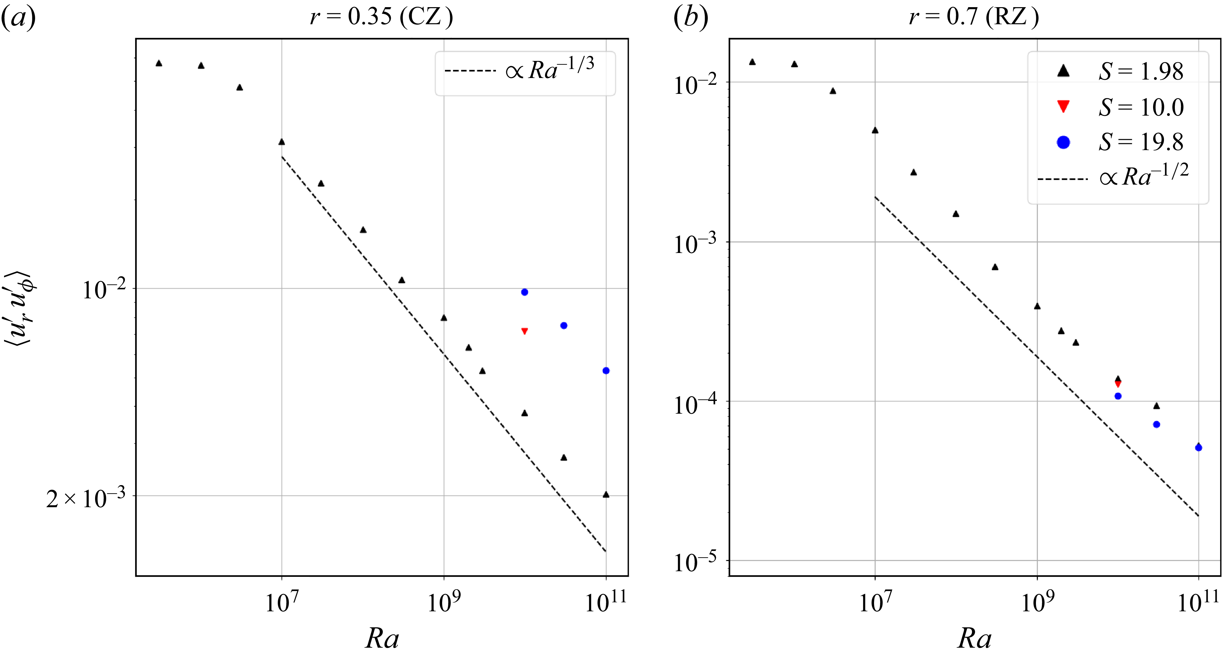
Note that to derive (4.3) and (4.4), we dropped order one factors. In figure 2(a), we plot $\langle u^{\prime}_r {u^{\prime}_\phi} \rangle$
in the CZ
$\langle u^{\prime}_r {u^{\prime}_\phi} \rangle$
in the CZ $(r=0.35)$
, where
$(r=0.35)$
, where $X'$
quantities are deviation from their azimuthal mean
$X'$
quantities are deviation from their azimuthal mean $\langle X\rangle$
. Note that
$\langle X\rangle$
. Note that $\langle u_r u_\phi \rangle = \langle u^{\prime}_r u^{\prime}_\phi\rangle$
as
$\langle u_r u_\phi \rangle = \langle u^{\prime}_r u^{\prime}_\phi\rangle$
as $\langle u_r\rangle =0$
. The plot shows good agreement with (4.3). In addition, there is a dependence on
$\langle u_r\rangle =0$
. The plot shows good agreement with (4.3). In addition, there is a dependence on $S$
, consistent with the earlier study of Couston et al. (Reference Couston, Lecoanet, Favier and Le Bars2017). They showed that convective plumes are enhanced for low-stiffness simulations, due to the fact that they can penetrate more easily in the radiative layer as
$S$
, consistent with the earlier study of Couston et al. (Reference Couston, Lecoanet, Favier and Le Bars2017). They showed that convective plumes are enhanced for low-stiffness simulations, due to the fact that they can penetrate more easily in the radiative layer as $N$
decreases with
$N$
decreases with $S$
(see (2.5)), consistent with our findings.
$S$
(see (2.5)), consistent with our findings.
The scaling laws (4.3) and (4.4) are predictions of the so-called ultimate or ‘Gallet’ regime of convection (Kraichnan Reference Kraichnan1962; Spiegel Reference Spiegel1963; Lepot, Aumaître & Gallet Reference Lepot, Aumaître and Gallet2018). The agreement between our simulations and these scaling laws is indeed not surprising as our convective model is similar to previous ones (Bouillaut et al. Reference Bouillaut, Lepot, Aumaître and Gallet2019; Hadjerci et al. Reference Hadjerci, Bouillaut, Miquel and Gallet2024) that demonstrated that for a volumetric heat source, molecular viscosity does not affect the Reynolds number or the heat transfer for flows with high enough $Ra$
. The ultimate regime is expected in problems with no thermal boundary layers (Lepot et al. Reference Lepot, Aumaître and Gallet2018). In our polar geometry, there is no bottom boundary at
$Ra$
. The ultimate regime is expected in problems with no thermal boundary layers (Lepot et al. Reference Lepot, Aumaître and Gallet2018). In our polar geometry, there is no bottom boundary at $r=0$
, and hence no bottom boundary layer. Furthermore, the CZ/RZ interface does not act as a thermal boundary layer because there are vertical motions across the interface, hence the flux is transported by a mix of convection and diffusion. Note that in our case, the thermal flux equilibrium between the two zones (Appendix A) prevents the spatially averaged temperature to drift in time, which therefore does not require any cooling (Lepot et al. Reference Lepot, Aumaître and Gallet2018). We can rewrite the scaling laws for velocity and temperature into the usual ones for the Reynolds number
$r=0$
, and hence no bottom boundary layer. Furthermore, the CZ/RZ interface does not act as a thermal boundary layer because there are vertical motions across the interface, hence the flux is transported by a mix of convection and diffusion. Note that in our case, the thermal flux equilibrium between the two zones (Appendix A) prevents the spatially averaged temperature to drift in time, which therefore does not require any cooling (Lepot et al. Reference Lepot, Aumaître and Gallet2018). We can rewrite the scaling laws for velocity and temperature into the usual ones for the Reynolds number $\textit{Re}= \widetilde {u_c} \widetilde {r_o}/\widetilde {\nu } \sim ( Ra_{\textit{eff}}/\textit{Pr} )^{1/2}$
and Nusselt number
$\textit{Re}= \widetilde {u_c} \widetilde {r_o}/\widetilde {\nu } \sim ( Ra_{\textit{eff}}/\textit{Pr} )^{1/2}$
and Nusselt number $\textit{Nu} \sim 1/T \sim ( Ra_{\textit{eff}}\,\textit{Pr} )^{1/2}$
, introducing an effective Rayleigh number
$\textit{Nu} \sim 1/T \sim ( Ra_{\textit{eff}}\,\textit{Pr} )^{1/2}$
, introducing an effective Rayleigh number $Ra_{\textit{eff}}=Ra\, {T}$
based on the temperature difference between the centre and the interface. Both scalings are indeed characteristic of the ultimate regime of convection. In other words, the dynamics of the CZ is fundamentally independent of molecular viscosity, which is expected for our set-up.
$Ra_{\textit{eff}}=Ra\, {T}$
based on the temperature difference between the centre and the interface. Both scalings are indeed characteristic of the ultimate regime of convection. In other words, the dynamics of the CZ is fundamentally independent of molecular viscosity, which is expected for our set-up.

Figure 2. Averaged Reynolds stress for different $Ra$
and
$Ra$
and $S$
, in (a) the CZ and (b) the RZ. Note that contributions from the mean flows have been removed, but keeping them gives the same results.
$S$
, in (a) the CZ and (b) the RZ. Note that contributions from the mean flows have been removed, but keeping them gives the same results.
In figure 2(b), we plot the same quantity $\langle u^{\prime}_r {u^{\prime}_\phi} \rangle$
in the stably stratified region (
$\langle u^{\prime}_r {u^{\prime}_\phi} \rangle$
in the stably stratified region ( $r=0.7$
). We find a steeper dependency with
$r=0.7$
). We find a steeper dependency with $Ra$
than in the CZ, with
$Ra$
than in the CZ, with $\langle u^{\prime}_r {u^{\prime}_\phi}\rangle \sim Ra^{-1/2}$
. It is possible to understand the observed behaviour from the theory of Lecoanet & Quataert (Reference Lecoanet and Quataert2013) (see also Goldreich & Kumar Reference Goldreich and Kumar1990; Couston et al. Reference Couston, Lecoanet, Favier and Le Bars2018b
). They make a theoretical prediction for the wave energy flux
$\langle u^{\prime}_r {u^{\prime}_\phi}\rangle \sim Ra^{-1/2}$
. It is possible to understand the observed behaviour from the theory of Lecoanet & Quataert (Reference Lecoanet and Quataert2013) (see also Goldreich & Kumar Reference Goldreich and Kumar1990; Couston et al. Reference Couston, Lecoanet, Favier and Le Bars2018b
). They make a theoretical prediction for the wave energy flux ${F}={u_r} {p}$
, which is conserved in the absence of dissipation (e.g. Lighthill & Lighthill Reference Lighthill and Lighthill1978; Le Saux et al. Reference Le Saux, Baraffe, Guillet, Vlaykov, Morison, Pratt, Constantino and Goffrey2023). Neglecting diffusive effects, they estimate the total wave energy flux to scale as
${F}={u_r} {p}$
, which is conserved in the absence of dissipation (e.g. Lighthill & Lighthill Reference Lighthill and Lighthill1978; Le Saux et al. Reference Le Saux, Baraffe, Guillet, Vlaykov, Morison, Pratt, Constantino and Goffrey2023). Neglecting diffusive effects, they estimate the total wave energy flux to scale as
 \begin{equation} {F} \sim u_c^3 \frac {\omega _c}{N}, \end{equation}
with ${u_c} \sim (Ra \textit{Pr} )^{-1/6}$
(see (4.3)) the typical velocity of the CZ, and
${u_c} \sim (Ra \textit{Pr} )^{-1/6}$
(see (4.3)) the typical velocity of the CZ, and $\omega _c$
the dominant frequency. We will now show that this prediction is consistent with the power law observed in figure 2(b). To do so, the pressure must be related to the azimuthal velocity, which is done by taking the horizontal derivative of the linearised horizontal component of (2.6) in the bulk of the RZ (no damping layer) and in the inviscid limit. Assuming that the most significant contribution comes from frequency
$\omega _c$
the dominant frequency. We will now show that this prediction is consistent with the power law observed in figure 2(b). To do so, the pressure must be related to the azimuthal velocity, which is done by taking the horizontal derivative of the linearised horizontal component of (2.6) in the bulk of the RZ (no damping layer) and in the inviscid limit. Assuming that the most significant contribution comes from frequency $\omega =\omega _c$
and horizontal wavenumber
$\omega =\omega _c$
and horizontal wavenumber $m=1$
leads to
$m=1$
leads to $p=r\omega u_\phi /m$
, which indeed gives
$p=r\omega u_\phi /m$
, which indeed gives
 \begin{equation} {u_r}{u_\phi }\sim \left ( Ra \textit{Pr}\right )^{-1/2}. \end{equation}
Thus, similarly to the CZ, the properties of the largest-amplitude waves, which dominate the total wave energy flux and total angular momentum flux, can be explained by diffusion-free arguments. Note that this does not necessarily apply to the entire spectrum of IGWs, as we discuss next.

Figure 3. Wave energy flux temporal spectra measurements for (a–c) varying $Ra$
, fixed
$Ra$
, fixed $S$
and (d–f) fixed
$S$
and (d–f) fixed $Ra$
, varying
$Ra$
, varying $S$
. Spectra are computed in the RZ (
$S$
. Spectra are computed in the RZ ( $r=0.7$
), and displayed for three values of the horizontal wavenumber. The dashed lines show comparisons with predictions by Lecoanet & Quataert (Reference Lecoanet and Quataert2013).
$r=0.7$
), and displayed for three values of the horizontal wavenumber. The dashed lines show comparisons with predictions by Lecoanet & Quataert (Reference Lecoanet and Quataert2013).
The dynamics of the waves generated in the CZ and propagating in the RZ can be further characterised by studying spectra. In figure 3, we show frequency spectra of the wave energy flux for simulations of varying $Ra$
(figures 3
a–c) and varying
$Ra$
(figures 3
a–c) and varying $S$
(figures 3
d–f). Reynolds stress or kinetic energy spectra display similar behaviours. Spectra are computed by conducting a double Fourier transform on
$S$
(figures 3
d–f). Reynolds stress or kinetic energy spectra display similar behaviours. Spectra are computed by conducting a double Fourier transform on $u_r$
and
$u_r$
and $p$
both along the azimuthal and time coordinates, at
$p$
both along the azimuthal and time coordinates, at $r=0.7$
, over one thermal diffusive time. To eliminate contamination from secular variation, we applied a temporal Hann window function. Here,
$r=0.7$
, over one thermal diffusive time. To eliminate contamination from secular variation, we applied a temporal Hann window function. Here, $m=1,2,3$
are the first three largest horizontal wavenumbers.
$m=1,2,3$
are the first three largest horizontal wavenumbers.
Focusing on figures 3(a–c), we observe that the different curves tend to collapse onto one another as the Rayleigh number is increased. (As $F$
is not a positive quantity, we display only positive values.) This behaviour is consistent with Anders et al. (Reference Anders2023): the shape of the spectra, which is the exciting mechanism for the reversing mean flow, converges for high-enough
$F$
is not a positive quantity, we display only positive values.) This behaviour is consistent with Anders et al. (Reference Anders2023): the shape of the spectra, which is the exciting mechanism for the reversing mean flow, converges for high-enough $Ra$
.
$Ra$
.
Figures 3(d–f) show that varying $S$
shifts the spectra to peak at lower frequencies. This can be understood qualitatively by recalling that an increased value of
$S$
shifts the spectra to peak at lower frequencies. This can be understood qualitatively by recalling that an increased value of $S$
corresponds to a higher value of
$S$
corresponds to a higher value of $N$
(§ 2), and hence to a larger separation between the convective frequency
$N$
(§ 2), and hence to a larger separation between the convective frequency $\omega _c$
and that of buoyancy
$\omega _c$
and that of buoyancy $N$
, as the
$N$
, as the $x$
-axis is normalised by
$x$
-axis is normalised by $N$
. Indeed, we observe that the typical width of the spectra for the highest value of
$N$
. Indeed, we observe that the typical width of the spectra for the highest value of $S$
considered (
$S$
considered ( $S=19.8$
, yellow curve) decreases compared to the lower case (
$S=19.8$
, yellow curve) decreases compared to the lower case ( $S=1.98$
, green curve), leading to spectra being more peaked. Note that the predictions of Lecoanet & Quataert (Reference Lecoanet and Quataert2013) assume
$S=1.98$
, green curve), leading to spectra being more peaked. Note that the predictions of Lecoanet & Quataert (Reference Lecoanet and Quataert2013) assume $\omega _c \ll N$
, whereas here we have
$\omega _c \ll N$
, whereas here we have $N/\omega _c$
at most
$N/\omega _c$
at most $3.16$
(for
$3.16$
(for $S=19.8$
). Indeed, we find that their predictions for the frequency spectra (dashed lines) are at best valid only for a small range of frequencies. Lecoanet & Quataert (Reference Lecoanet and Quataert2013) also assume three-dimensional turbulence, though Lecoanet et al. (Reference Lecoanet, Cantiello, Anders, Quataert, Couston, Bouffard, Favier and Le Bars2021) find similar spectra in two-dimensional Cartesian simulations. The other important point is that their prediction is derived in the inviscid case. Finally, there are peaks slightly below
$S=19.8$
). Indeed, we find that their predictions for the frequency spectra (dashed lines) are at best valid only for a small range of frequencies. Lecoanet & Quataert (Reference Lecoanet and Quataert2013) also assume three-dimensional turbulence, though Lecoanet et al. (Reference Lecoanet, Cantiello, Anders, Quataert, Couston, Bouffard, Favier and Le Bars2021) find similar spectra in two-dimensional Cartesian simulations. The other important point is that their prediction is derived in the inviscid case. Finally, there are peaks slightly below $\omega = N$
corresponding to standing modes that have not been completely removed by the damping layer (Lecoanet et al. Reference Lecoanet, Cantiello, Anders, Quataert, Couston, Bouffard, Favier and Le Bars2021; Anders et al. Reference Anders2023).
$\omega = N$
corresponding to standing modes that have not been completely removed by the damping layer (Lecoanet et al. Reference Lecoanet, Cantiello, Anders, Quataert, Couston, Bouffard, Favier and Le Bars2021; Anders et al. Reference Anders2023).
Using these results, we can estimate the value of $\varLambda _1$
in our simulations. Rewriting (3.3) using the dimensionless parameters of the DNS gives
$\varLambda _1$
in our simulations. Rewriting (3.3) using the dimensionless parameters of the DNS gives
 \begin{equation} \varLambda _1 = \frac {1+\textit{Pr}}{Ra} \frac {1}{\langle {u^{\prime}_r}{u^{\prime}_\phi}\rangle }\left (\frac {N}{\overline {\omega }}\right )^3\overline {k}^2. \end{equation}
We have that $\varLambda _1$
depends on three simulation outputs: the angular momentum flux
$\varLambda _1$
depends on three simulation outputs: the angular momentum flux $\langle {u^{\prime}_r}{u^{\prime}_\phi}\rangle$
, the frequency ratio
$\langle {u^{\prime}_r}{u^{\prime}_\phi}\rangle$
, the frequency ratio $N/\overline {\omega }$
, and the average azimuthal wavenumber
$N/\overline {\omega }$
, and the average azimuthal wavenumber $\overline {k}$
. Here,
$\overline {k}$
. Here, $\overline {X}$
denotes weighted averages (see below). In figure 2 and (4.6), we show the strong dependence of
$\overline {X}$
denotes weighted averages (see below). In figure 2 and (4.6), we show the strong dependence of $\langle {u^{\prime}_r}{u^{\prime}_\phi}\rangle$
on
$\langle {u^{\prime}_r}{u^{\prime}_\phi}\rangle$
on $Ra$
and
$Ra$
and $\textit{Pr}$
. To first order, the ratio
$\textit{Pr}$
. To first order, the ratio $N/\overline {\omega }$
is determined by
$N/\overline {\omega }$
is determined by $S$
, and
$S$
, and $\overline {k}$
corresponds to the dominant mode of the CZ, which is
$\overline {k}$
corresponds to the dominant mode of the CZ, which is $m=1$
in our simulations. Note that this reasoning holds for the maxima of spectra, which can be quite dispersed. Here, we rather measured the typical frequencies and azimuthal wavenumbers by conducting weighted averages of the spectra presented in figure 3 in the corresponding direction (see Appendix B), namely
$m=1$
in our simulations. Note that this reasoning holds for the maxima of spectra, which can be quite dispersed. Here, we rather measured the typical frequencies and azimuthal wavenumbers by conducting weighted averages of the spectra presented in figure 3 in the corresponding direction (see Appendix B), namely $\overline {\omega }\equiv \langle |\omega F |\rangle / \langle | F |\rangle$
and
$\overline {\omega }\equiv \langle |\omega F |\rangle / \langle | F |\rangle$
and $\overline {k}\equiv \langle |m F |\rangle / (\langle | F |\rangle /0.7)$
– we recall that
$\overline {k}\equiv \langle |m F |\rangle / (\langle | F |\rangle /0.7)$
– we recall that $F$
is measured at
$F$
is measured at $r=0.7$
. It enables us to obtain a more useful measure of
$r=0.7$
. It enables us to obtain a more useful measure of $\varLambda _1$
. Using (4.6), we predict that
$\varLambda _1$
. Using (4.6), we predict that $\varLambda _1$
decreases like
$\varLambda _1$
decreases like ${Ra}^{-1/2}$
at fixed
${Ra}^{-1/2}$
at fixed $S$
and
$S$
and $\textit{Pr}$
. While we recover this scaling for low
$\textit{Pr}$
. While we recover this scaling for low $Ra$
, at higher
$Ra$
, at higher $Ra$
, we find
$Ra$
, we find $\varLambda \propto Ra^{-1/3}$
. As we showed in figure 2(b) that
$\varLambda \propto Ra^{-1/3}$
. As we showed in figure 2(b) that $\langle u^{\prime}_r u^{\prime}_\phi \rangle \propto Ra^{-1/2}$
,
$\langle u^{\prime}_r u^{\prime}_\phi \rangle \propto Ra^{-1/2}$
, $\varLambda _1 \propto Ra^{-1/3}$
means that
$\varLambda _1 \propto Ra^{-1/3}$
means that $\overline {k}$
or
$\overline {k}$
or $\overline {\omega }$
depends on
$\overline {\omega }$
depends on $Ra$
(see Appendix B). This may be explained by the way in which we measure
$Ra$
(see Appendix B). This may be explained by the way in which we measure $\overline {k}$
and
$\overline {k}$
and $\overline {\omega }$
. Nevertheless, increasing
$\overline {\omega }$
. Nevertheless, increasing $Ra$
decreases
$Ra$
decreases $\varLambda _1$
until it becomes smaller than
$\varLambda _1$
until it becomes smaller than $\varLambda _1^c$
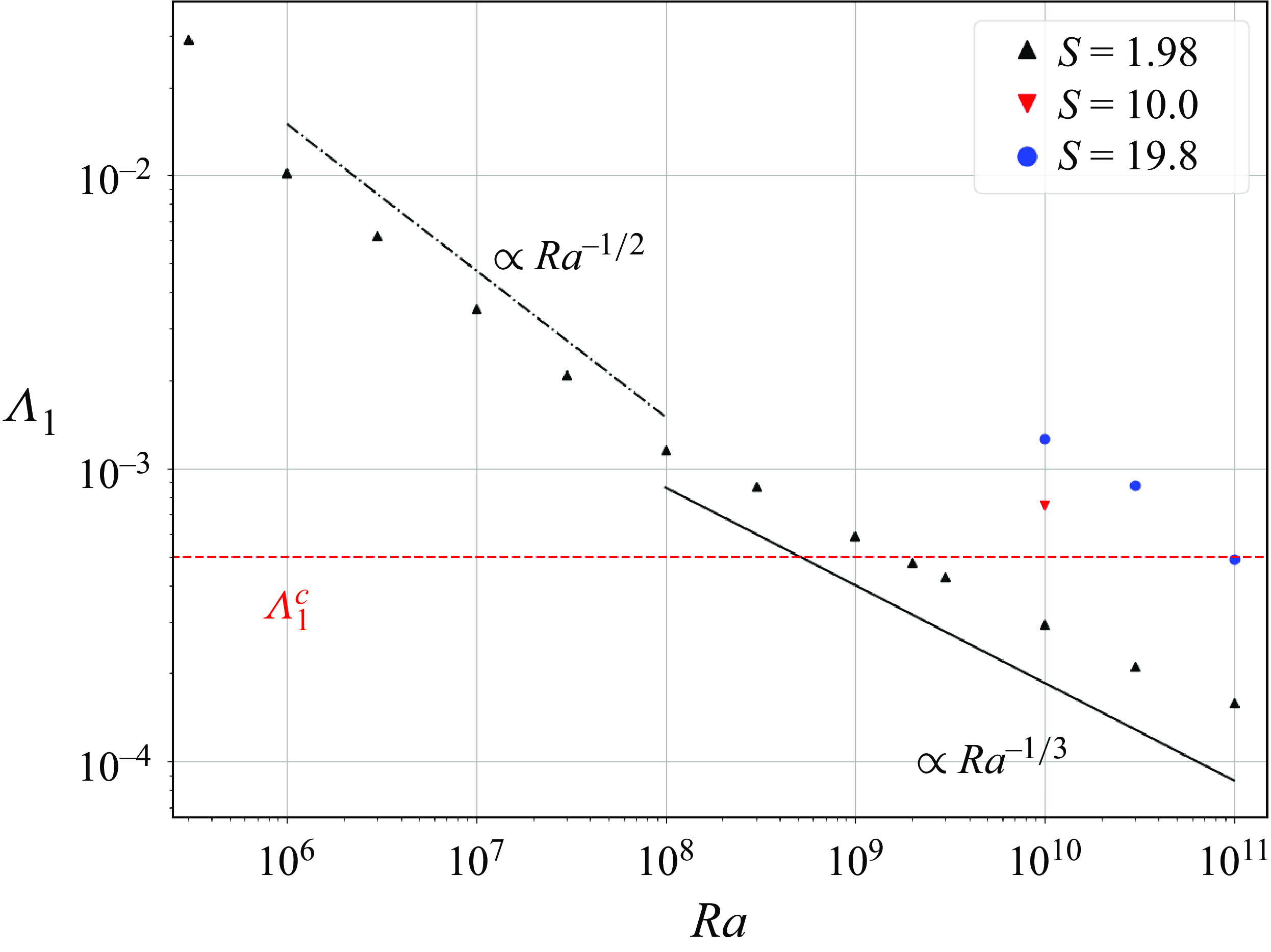
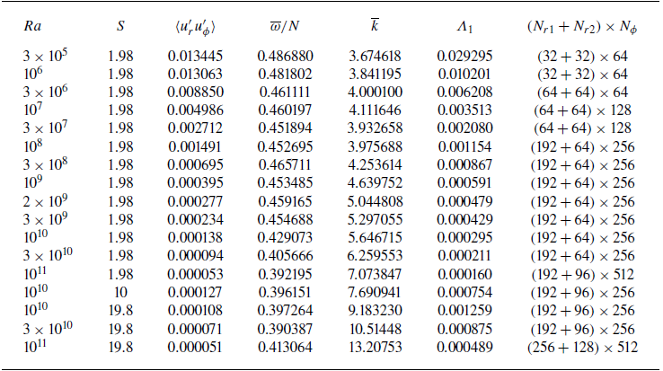
. We estimate
$\varLambda _1^c$
. We estimate $\varLambda _1^c\approx 5\times10^{-4}$
in the simulations (red line of figure 4). The system is then beyond the onset of a reversing mean flow, i.e. the Rayleigh number is higher than a critical Rayleigh number. Higher values of
$\varLambda _1^c\approx 5\times10^{-4}$
in the simulations (red line of figure 4). The system is then beyond the onset of a reversing mean flow, i.e. the Rayleigh number is higher than a critical Rayleigh number. Higher values of $S$
, while increasing the corresponding values of critical Rayleigh numbers, does not affect the picture. Note that (4.7) gives some weight to the interpretation of Couston et al. (Reference Couston, Lecoanet, Favier and Le Bars2018a
) who observed favoured mean flows for low Prandtl simulations, as
$S$
, while increasing the corresponding values of critical Rayleigh numbers, does not affect the picture. Note that (4.7) gives some weight to the interpretation of Couston et al. (Reference Couston, Lecoanet, Favier and Le Bars2018a
) who observed favoured mean flows for low Prandtl simulations, as $\varLambda _1 \propto \sqrt {\textit{Pr}}\,(1+\textit{Pr})$
. On the contrary, laboratory experiments conducted by Semin et al. (Reference Semin, Garroum, Pétrélis and Fauve2018) led to mean flow reversals using salt stratification, for which the value of the equivalent quantity – the Schmidt number – is rather approximately
$\varLambda _1 \propto \sqrt {\textit{Pr}}\,(1+\textit{Pr})$
. On the contrary, laboratory experiments conducted by Semin et al. (Reference Semin, Garroum, Pétrélis and Fauve2018) led to mean flow reversals using salt stratification, for which the value of the equivalent quantity – the Schmidt number – is rather approximately $700$
. This suggests that the quantity that determines the properties of the mean flow evolution is
$700$
. This suggests that the quantity that determines the properties of the mean flow evolution is $\varLambda _1$
rather than
$\varLambda _1$
rather than $\textit{Pr}$
. Semin et al. (Reference Semin, Garroum, Pétrélis and Fauve2018) showed that their results could be explained by varying
$\textit{Pr}$
. Semin et al. (Reference Semin, Garroum, Pétrélis and Fauve2018) showed that their results could be explained by varying $\varLambda _1$
, and we find similar results in our simulations.
$\varLambda _1$
, and we find similar results in our simulations.


4.2. Reversing mean flows
In figure 5, we visualise the mean flows generated in simulations with $S=1.98$
and
$S=1.98$
and $Ra\in \{10^{10},3\times10^{10},10^{11}\}$
. These correspond to simulations where
$Ra\in \{10^{10},3\times10^{10},10^{11}\}$
. These correspond to simulations where $\varLambda _1$
has become small enough for a mean flow to develop, in agreement with the discussion of § 4.1 and figure 4.
$\varLambda _1$
has become small enough for a mean flow to develop, in agreement with the discussion of § 4.1 and figure 4.

Figure 5. Mean flow visualisation for $S=1.98$
: (a,c,e) Hovmöller diagrams (colours correspond to flow amplitudes) and (b,d, f) phase portraits of local probes of the zonal velocity in the RZ (colours correspond to time) for (a,b)
$S=1.98$
: (a,c,e) Hovmöller diagrams (colours correspond to flow amplitudes) and (b,d, f) phase portraits of local probes of the zonal velocity in the RZ (colours correspond to time) for (a,b) $Ra=10^{10}$
, (c,d)
$Ra=10^{10}$
, (c,d) $Ra=3\times10^{10}$
and (e,f)
$Ra=3\times10^{10}$
and (e,f) $Ra=10^{11}$
.
$Ra=10^{11}$
.
In figures 5(a,c,e), we plot Hovmöller diagrams showing the zonally averaged azimuthal velocity $\langle {u_\phi }\rangle$
as a function of both space and time. This is a classical type of representation of the problem (see e.g. Wedi & Smolarkiewicz Reference Wedi and Smolarkiewicz2006), which illustrates how the pattern of the flow evolves. Focusing on figure 5(a), we can describe the velocity evolution. At
$\langle {u_\phi }\rangle$
as a function of both space and time. This is a classical type of representation of the problem (see e.g. Wedi & Smolarkiewicz Reference Wedi and Smolarkiewicz2006), which illustrates how the pattern of the flow evolves. Focusing on figure 5(a), we can describe the velocity evolution. At $t=0$
(note that this simulation was initialised with the final state of the
$t=0$
(note that this simulation was initialised with the final state of the $Ra=3\times10^9$
simulation), the mean flow is negative at lower radii in the RZ, and positive at higher radii in the RZ. We will next discuss the propagation and angular momentum transport of first the prograde (positive phase velocity) waves, and then the retrograde (negative phase velocity) waves. Prograde IGWs propagate from the CZ/RZ interface towards the top of the layer. They are absorbed by the medium at a relatively high radius where their absorption leads to a local acceleration of the flow. As time goes by (until
$Ra=3\times10^9$
simulation), the mean flow is negative at lower radii in the RZ, and positive at higher radii in the RZ. We will next discuss the propagation and angular momentum transport of first the prograde (positive phase velocity) waves, and then the retrograde (negative phase velocity) waves. Prograde IGWs propagate from the CZ/RZ interface towards the top of the layer. They are absorbed by the medium at a relatively high radius where their absorption leads to a local acceleration of the flow. As time goes by (until $t\approx 0.5 \tau _\kappa$
), the absorption process occurs lower as the waves are preferentially absorbed when
$t\approx 0.5 \tau _\kappa$
), the absorption process occurs lower as the waves are preferentially absorbed when $\langle u_\phi \rangle \sim c$
(see e.g. (3.2)). This leads to the mean flow propagating downwards and even penetrating into the CZ. While these prograde waves are subsequently absorbed at lower radii, retrograde waves are not filtered by the positive mean flow and are able to propagate in the RZ to deposit their angular momentum, with a blue patch that starts to appear at high radii at
$\langle u_\phi \rangle \sim c$
(see e.g. (3.2)). This leads to the mean flow propagating downwards and even penetrating into the CZ. While these prograde waves are subsequently absorbed at lower radii, retrograde waves are not filtered by the positive mean flow and are able to propagate in the RZ to deposit their angular momentum, with a blue patch that starts to appear at high radii at $t\approx 0.2 \tau _\kappa$
. It is the alternation between the absorption processes of prograde and retrograde waves that gives birth to the observed large-scale oscillation that repeats afterwards. It is in good agreement with reduced models; the main difference here is that the spectrum of waves is continuous (figure 3). Note that the typical period of mean flow reversals is comparable to the thermal diffusion time, i.e. much longer than the convective turnover time (see the rapid variations in the CZ). Similar results were obtained by Couston et al. (Reference Couston, Lecoanet, Favier and Le Bars2018a
) in Cartesian geometry. This phenomenon is also observed in figures 5(c,e), but the pattern described before is different. Indeed, for the highest
$t\approx 0.2 \tau _\kappa$
. It is the alternation between the absorption processes of prograde and retrograde waves that gives birth to the observed large-scale oscillation that repeats afterwards. It is in good agreement with reduced models; the main difference here is that the spectrum of waves is continuous (figure 3). Note that the typical period of mean flow reversals is comparable to the thermal diffusion time, i.e. much longer than the convective turnover time (see the rapid variations in the CZ). Similar results were obtained by Couston et al. (Reference Couston, Lecoanet, Favier and Le Bars2018a
) in Cartesian geometry. This phenomenon is also observed in figures 5(c,e), but the pattern described before is different. Indeed, for the highest $Ra$
reported (figure 5
e), the mean flow has a modified shape, which we interpret as the transition towards a quasi-periodic behaviour. Shorter reversals of the flows can be seen close to the CZ/RZ interface. This is expected in the Plumb–McEwan model (Kim & MacGregor Reference Kim and MacGregor2001; Renaud et al. Reference Renaud, Nadeau and Venaille2019) when
$Ra$
reported (figure 5
e), the mean flow has a modified shape, which we interpret as the transition towards a quasi-periodic behaviour. Shorter reversals of the flows can be seen close to the CZ/RZ interface. This is expected in the Plumb–McEwan model (Kim & MacGregor Reference Kim and MacGregor2001; Renaud et al. Reference Renaud, Nadeau and Venaille2019) when $\varLambda _1$
is sufficiently reduced, but here we report a clear example with a self-consistent wave spectrum. Note that Chartrand et al. (Reference Chartrand, Nadeau and Venaille2024) attribute this transition to a quasi-periodic regime by the emergence of new unstable modes in the linearised problem of § 3. The comparison is nevertheless complicated by the stochastic nature of the current problem, and is left for future work.
$\varLambda _1$
is sufficiently reduced, but here we report a clear example with a self-consistent wave spectrum. Note that Chartrand et al. (Reference Chartrand, Nadeau and Venaille2024) attribute this transition to a quasi-periodic regime by the emergence of new unstable modes in the linearised problem of § 3. The comparison is nevertheless complicated by the stochastic nature of the current problem, and is left for future work.

Figure 6. Same as in figure 5 but for $Ra=10^{10}$
: (a,b)
$Ra=10^{10}$
: (a,b) $S=1.98$
, (c,d)
$S=1.98$
, (c,d) $S=10$
and (e, f)
$S=10$
and (e, f) $S=19.8$
.
$S=19.8$
.
In figures 5(b,d, f), we plot phase portraits of two local probes of the flow at $r=0.7$
and
$r=0.7$
and $r=0.8$
. Phase portraits show the emergence of limit cycles and their regularity (Kim & MacGregor Reference Kim and MacGregor2001). Combining these two representations illustrates how increasing
$r=0.8$
. Phase portraits show the emergence of limit cycles and their regularity (Kim & MacGregor Reference Kim and MacGregor2001). Combining these two representations illustrates how increasing $Ra$
affects the evolution of the flow: the shape shown in figure 5(b) displays a regular limit cycle, in agreement with the Hovmöller diagram shown in figure 5(a). There is a single orbit as the flow is periodic. Note the short time scale fluctuations clearly visible in this representation, attributable to fluctuations due to the CZ. The orbit is, however, modified in figures 5(d, f) as
$Ra$
affects the evolution of the flow: the shape shown in figure 5(b) displays a regular limit cycle, in agreement with the Hovmöller diagram shown in figure 5(a). There is a single orbit as the flow is periodic. Note the short time scale fluctuations clearly visible in this representation, attributable to fluctuations due to the CZ. The orbit is, however, modified in figures 5(d, f) as $Ra$
is increased, with limit cycles exhibiting now a more complex shape. In figure 5(f), the phase portrait is expected to fill in a torus as the flow is quasi-periodic. Thus increasing
$Ra$
is increased, with limit cycles exhibiting now a more complex shape. In figure 5(f), the phase portrait is expected to fill in a torus as the flow is quasi-periodic. Thus increasing $Ra$
maintains reversals while modifying the period of the flow.
$Ra$
maintains reversals while modifying the period of the flow.
In figure 6, we visualise the mean flows generated in simulations with $Ra=10^{10}$
and
$Ra=10^{10}$
and $S \in \{1.98,10,19.8\}$
. While, as shown above, we find regular mean flow oscillations for low
$S \in \{1.98,10,19.8\}$
. While, as shown above, we find regular mean flow oscillations for low $S$
(figures 6
a,b), increasing
$S$
(figures 6
a,b), increasing $S$
causes the mean flow evolution to become increasingly irregular (figures 6
c–f). That said, the mean flow still exhibits downward-propagating patterns for higher values of
$S$
causes the mean flow evolution to become increasingly irregular (figures 6
c–f). That said, the mean flow still exhibits downward-propagating patterns for higher values of $S$
. We expect that simulations with
$S$
. We expect that simulations with $S=10$
or
$S=10$
or $S=19.8$
would exhibit regular mean flows similar to the
$S=19.8$
would exhibit regular mean flows similar to the $S=1.98$
simulations if they are run with higher
$S=1.98$
simulations if they are run with higher $Ra$
corresponding to
$Ra$
corresponding to $\varLambda _1$
sufficiently below
$\varLambda _1$
sufficiently below $\varLambda _1^c$
(see figure 4). Note that in figure 5, we plot the mean flow evolution for two thermal times, whereas in figure 6, we plot the mean flow evolution for
$\varLambda _1^c$
(see figure 4). Note that in figure 5, we plot the mean flow evolution for two thermal times, whereas in figure 6, we plot the mean flow evolution for $1.5$
thermal times. This is in part due to computational constraints, as higher
$1.5$
thermal times. This is in part due to computational constraints, as higher $S$
simulations require higher vertical resolution.
$S$
simulations require higher vertical resolution.
Next we turn our attention to the period of the mean flow oscillations. We measure the period $T_{\textit{osc}}$
by finding the frequency of the highest-amplitude peak of the Fourier transform of
$T_{\textit{osc}}$
by finding the frequency of the highest-amplitude peak of the Fourier transform of $u_\phi (r=0.65)$
. We find that
$u_\phi (r=0.65)$
. We find that $T_{\textit{osc}}$
is insensitive to the choice of radius. We plot
$T_{\textit{osc}}$
is insensitive to the choice of radius. We plot $T_{\textit{osc}}$
for each of our simulations in figure 7(a). Simulations without coherent mean flow oscillations (
$T_{\textit{osc}}$
for each of our simulations in figure 7(a). Simulations without coherent mean flow oscillations ( $\varLambda _1\gt \varLambda _1^c$
) correspond to cases where a regular mean flow is difficult to observe, but nevertheless exhibit some activities in their RZ. We also plot with a dashed line
$\varLambda _1\gt \varLambda _1^c$
) correspond to cases where a regular mean flow is difficult to observe, but nevertheless exhibit some activities in their RZ. We also plot with a dashed line $T_{\textit{osc}} \propto \tau _{\kappa }=\sqrt {Ra \textit{Pr}}$
, following the observations of figure 5 where the two time scales appear to be connected. Indeed, expressing
$T_{\textit{osc}} \propto \tau _{\kappa }=\sqrt {Ra \textit{Pr}}$
, following the observations of figure 5 where the two time scales appear to be connected. Indeed, expressing $\widetilde {T_{\textit{osc}}} \sim \widetilde {c}\widetilde {d}/\widetilde {L}$
in the DNS non-dimensionalisation leads to
$\widetilde {T_{\textit{osc}}} \sim \widetilde {c}\widetilde {d}/\widetilde {L}$
in the DNS non-dimensionalisation leads to
 \begin{equation} T_{\textit{osc}} \sim \left ( \frac {\overline {\omega }}{N} \right )^5\frac {N^2}{\overline {k} ^4}\frac {\sqrt {Ra \textit{Pr}}}{1+\textit{Pr}}\frac {1}{\langle {u^{\prime}_r}{u^{\prime}_\phi}\rangle }\equiv X_T. \end{equation}
In figure 7(b), we plot $T_{\textit{osc}}$
as a function of
$T_{\textit{osc}}$
as a function of $X_T$
, showing that the simulations agree well with (4.8). The combination of the dependencies of both
$X_T$
, showing that the simulations agree well with (4.8). The combination of the dependencies of both $\langle u^{\prime}_r u^{\prime}_\phi \rangle$
and
$\langle u^{\prime}_r u^{\prime}_\phi \rangle$
and $\tau _\kappa$
on
$\tau _\kappa$
on $Ra$
and
$Ra$
and $\textit{Pr}$
leads to
$\textit{Pr}$
leads to $T_{\textit{osc}}\propto (Ra \textit{Pr})^1$
. The diffusive time scale constrains the oscillation of the mean flow through the typical damping length of the waves, which for low-
$T_{\textit{osc}}\propto (Ra \textit{Pr})^1$
. The diffusive time scale constrains the oscillation of the mean flow through the typical damping length of the waves, which for low- $\textit{Pr}$
fluids is dominated by thermal diffusion. Equation (4.8) was derived in the framework of the Hopf bifurcation, which means that in the vicinity of the threshold,
$\textit{Pr}$
fluids is dominated by thermal diffusion. Equation (4.8) was derived in the framework of the Hopf bifurcation, which means that in the vicinity of the threshold, ${T_{\textit{osc}}^{\text{1-D}}}\sim O(1)$
; recall that the one-dimensional (1-D) model and DNS have different units. Besides showing the good agreement with earlier reduced models, our DNS allow us to compute the prefactor in (4.8),
${T_{\textit{osc}}^{\text{1-D}}}\sim O(1)$
; recall that the one-dimensional (1-D) model and DNS have different units. Besides showing the good agreement with earlier reduced models, our DNS allow us to compute the prefactor in (4.8), $T_{\textit{osc}}=4X_T$
.
$T_{\textit{osc}}=4X_T$
.

Figure 7. Dominant period evolution. (a) Measurement in our data set via Fourier transform (see text for details) as a function of $Ra$
for several
$Ra$
for several $S$
. (b) Same as (a) but as a function of
$S$
. (b) Same as (a) but as a function of $X_T$
(see (4.8)). Simulations for which
$X_T$
(see (4.8)). Simulations for which $\varLambda _1$
is higher than
$\varLambda _1$
is higher than $\varLambda _1^c$
are reported as empty symbols.
$\varLambda _1^c$
are reported as empty symbols.

Figure 8. Mean flow velocity evolution. (a) Root mean square of the RZ zonal velocity (measured from $r=0.6$
to
$r=0.6$
to $r=1$
in our data set) as a function of
$r=1$
in our data set) as a function of $Ra$
for several
$Ra$
for several $S$
. (b) Plot of
$S$
. (b) Plot of $u_{\textit{rms}}^{\textit{RZ}}/c={u}_{\textit{rms}}^{\textit{RZ}}/(\overline {\omega }/\overline {k} )$
(see text for details) against the distance from the onset
$u_{\textit{rms}}^{\textit{RZ}}/c={u}_{\textit{rms}}^{\textit{RZ}}/(\overline {\omega }/\overline {k} )$
(see text for details) against the distance from the onset $\varepsilon =(\varLambda _1^c-\varLambda _1)/\varLambda _1$
.
$\varepsilon =(\varLambda _1^c-\varLambda _1)/\varLambda _1$
.
The Plumb–McEwan model also makes predictions for the velocity amplitude of the mean flow. Figure 8(a) shows the root mean square zonal velocity $\langle {u_\phi }\rangle$
in the RZ as a function of
$\langle {u_\phi }\rangle$
in the RZ as a function of $Ra$
for several
$Ra$
for several $S$
. On the one hand, for
$S$
. On the one hand, for $S=1.98$
, the flow increases in amplitude until
$S=1.98$
, the flow increases in amplitude until $Ra=10^{10}$
. We can interpret this in terms of the 1-D model for which the control parameter is
$Ra=10^{10}$
. We can interpret this in terms of the 1-D model for which the control parameter is $1/\varLambda _1$
. Thus for this Hopf bifurcation, we expect the velocity to increase as the square root of the supercriticality, i.e.
$1/\varLambda _1$
. Thus for this Hopf bifurcation, we expect the velocity to increase as the square root of the supercriticality, i.e. $u^{\textit{RZ}}_{\textit{rms}}/c \propto \sqrt {(\varLambda _1^c-\varLambda _1)/\varLambda _1}\equiv \sqrt {\varepsilon }$
. We show in figure 8(b) that this is consistent with the three lowest
$u^{\textit{RZ}}_{\textit{rms}}/c \propto \sqrt {(\varLambda _1^c-\varLambda _1)/\varLambda _1}\equiv \sqrt {\varepsilon }$
. We show in figure 8(b) that this is consistent with the three lowest $Ra$
at
$Ra$
at $S=1.98$
, though this result is very sensitive to the precise value of
$S=1.98$
, though this result is very sensitive to the precise value of $\varLambda _1^c$
. However, for larger
$\varLambda _1^c$
. However, for larger $Ra\gt 10^{10}$
, we find smaller-amplitude mean flows, which we attribute to the emergence of new patterns and the transition towards a quasi-periodic state. Note that what appears to be a secondary transition between
$Ra\gt 10^{10}$
, we find smaller-amplitude mean flows, which we attribute to the emergence of new patterns and the transition towards a quasi-periodic state. Note that what appears to be a secondary transition between $Ra=10^{10}$
and
$Ra=10^{10}$
and $Ra=3\times10^{10}$
could be due to the fact that the wave damping length starts to be comparable to the size of the RZ, as it reads
$Ra=3\times10^{10}$
could be due to the fact that the wave damping length starts to be comparable to the size of the RZ, as it reads $\widetilde{d}/(\widetilde{r_o}-\widetilde{r_i}) = (\overline{\omega}/N)^4 (N/\overline{k}^3)\sqrt{RaPr}/ ((1+Pr)(1-r_i))$
. Chartrand et al. (Reference Chartrand, Nadeau and Venaille2024) indeed showed that more complex bifurcations could occur when this is the case, which could account for the non-monotonic velocity variations with
$\widetilde{d}/(\widetilde{r_o}-\widetilde{r_i}) = (\overline{\omega}/N)^4 (N/\overline{k}^3)\sqrt{RaPr}/ ((1+Pr)(1-r_i))$
. Chartrand et al. (Reference Chartrand, Nadeau and Venaille2024) indeed showed that more complex bifurcations could occur when this is the case, which could account for the non-monotonic velocity variations with $Ra$
in the present work. On the other hand, increasing
$Ra$
in the present work. On the other hand, increasing $S$
seems to reduce the amplitude of the flow through a higher value of the Brunt–Väisälä frequency.
$S$
seems to reduce the amplitude of the flow through a higher value of the Brunt–Väisälä frequency.
We want to emphasise the striking finding of our paper that DNS, although involving a continuous spectrum of IGWs due to the CZ, are well captured by the Plumb–McEwan model. It hints that spectra, through their dominant frequency, act as an effective monochromatic forcing. This point should, however, be nuanced, and remains qualitative, particularly for the velocity. The ability of the reduced model to quantitatively compare to global simulations outputs was tested by Couston et al. (Reference Couston, Lecoanet, Favier and Le Bars2018a
), who extracted DNS spectra of various frequencies and horizontal wavenumbers. Concretely, it consists in integrating numerically the model of § 3 while summing contributions of the Reynolds stress (3.2) from several waves, taking for the prefactors the values measured in DNS. While they were able to reproduce mean flow reversals with this mixed DNS/Plumb–McEwan model, the comparison was not perfect. One possible reason could be that, as in our case, the important level of fluctuations due to the CZ limits the comparison with the 1-D model. Indeed (see § 3), the latter considers deterministic dynamics, i.e. neglects any stochastic processes. We posit that the fluctuations of the CZ, for instance acting through temporal variations of $\langle {u^{\prime}_r} {u^{\prime}_\phi}\rangle$
, affects the classical picture. Their effect could be thought of as a multiplicative noise, which we discuss in § 5. The present point is that in the perspective of understanding the system as resulting from a Hopf bifurcation, the notion of a threshold only makes sense statistically. This may explain why the run at
$\langle {u^{\prime}_r} {u^{\prime}_\phi}\rangle$
, affects the classical picture. Their effect could be thought of as a multiplicative noise, which we discuss in § 5. The present point is that in the perspective of understanding the system as resulting from a Hopf bifurcation, the notion of a threshold only makes sense statistically. This may explain why the run at $S=10$
,
$S=10$
, $Ra=10^{10}$
has
$Ra=10^{10}$
has $\varLambda _1\gt \varLambda _1^c$
(see Appendix B), i.e. should be classified as stable, but nevertheless exhibits features (see again figure 6
c) that are typical of a reversing mean flow. Fluctuations are also apparent in the phase portraits of figures 5 and 6 where noise superimposed to limit cycles is clearly visible.
$\varLambda _1\gt \varLambda _1^c$
(see Appendix B), i.e. should be classified as stable, but nevertheless exhibits features (see again figure 6
c) that are typical of a reversing mean flow. Fluctuations are also apparent in the phase portraits of figures 5 and 6 where noise superimposed to limit cycles is clearly visible.

Figure 9. Temporal behaviours of the mean flow. (a) Local probes of the zonally averaged velocity at $r=0.65$
as a function of time for
$r=0.65$
as a function of time for $Ra=10^{10}$
and
$Ra=10^{10}$
and $Ra=10^{11}$
, both at
$Ra=10^{11}$
, both at $S=1.98$
. (b) Corresponding Fourier transform for the signals reported in (a). The
$S=1.98$
. (b) Corresponding Fourier transform for the signals reported in (a). The $x$
-axis is normalised by the value of the dominant frequency in each case.
$x$
-axis is normalised by the value of the dominant frequency in each case.
In figure 9(a), we show $\langle {u_\phi } \rangle (r=0.65)$
for the simulations
$\langle {u_\phi } \rangle (r=0.65)$
for the simulations $S=1.98$
,
$S=1.98$
, $Ra=10^{10}$
and
$Ra=10^{10}$
and $Ra=10^{11}$
, corresponding to the Hovmöller diagrams reported in figures 5(a) and 5(e). We use these data to measure the mean flow oscillation periods. We show the corresponding Fourier transform in figure 9(b). The time series illustrate the time scale separation that is at the basis of past reduced models. Convective motions produce variations on time scales
$Ra=10^{11}$
, corresponding to the Hovmöller diagrams reported in figures 5(a) and 5(e). We use these data to measure the mean flow oscillation periods. We show the corresponding Fourier transform in figure 9(b). The time series illustrate the time scale separation that is at the basis of past reduced models. Convective motions produce variations on time scales $O(1)$
. It is these rapid variations that lead to the much longer oscillation of
$O(1)$
. It is these rapid variations that lead to the much longer oscillation of $O(10^4)$
corresponding to the reversing mean flow. In figure 9(b), the Fourier transforms exhibit two clear peaks. Interestingly, even the peak-to-peak amplitude fluctuates, as the results of the CZ noise discussed earlier. We also see that the typical mean flow velocity decreases as
$O(10^4)$
corresponding to the reversing mean flow. In figure 9(b), the Fourier transforms exhibit two clear peaks. Interestingly, even the peak-to-peak amplitude fluctuates, as the results of the CZ noise discussed earlier. We also see that the typical mean flow velocity decreases as $Ra$
increases (figure 8
b). Our interpretation is that the system undergoes a second transition in this case, leading to the emergence of a second noticeable peak in the Fourier transform. Indeed, a higher frequency emerges on the red curve of figure 9(b), which seems to be situated between
$Ra$
increases (figure 8
b). Our interpretation is that the system undergoes a second transition in this case, leading to the emergence of a second noticeable peak in the Fourier transform. Indeed, a higher frequency emerges on the red curve of figure 9(b), which seems to be situated between $3f_{\textit{max}}$
and
$3f_{\textit{max}}$
and $4f_{\textit{max}}$
. The fact that it does not correspond to an integer multiple of
$4f_{\textit{max}}$
. The fact that it does not correspond to an integer multiple of $f_{\textit{max}}$
suggests the transition to a quasi-periodic regime, as one would rather expect clear harmonics – integer multiples of
$f_{\textit{max}}$
suggests the transition to a quasi-periodic regime, as one would rather expect clear harmonics – integer multiples of $f_{\textit{max}}$
– if the system were to remain periodic. This is compatible with the temporal probe of figure 9(a), which exhibits shorter oscillations between each global extremum, which are absent for
$f_{\textit{max}}$
– if the system were to remain periodic. This is compatible with the temporal probe of figure 9(a), which exhibits shorter oscillations between each global extremum, which are absent for $Ra=10^{10}$
, as well as with figure 5(e), where shorter oscillations appear at
$Ra=10^{10}$
, as well as with figure 5(e), where shorter oscillations appear at $r=0.65$
.
$r=0.65$
.
We also report a third peak lower than $f_{\textit{max}}$
for the
$f_{\textit{max}}$
for the $Ra=10^{11}$
simulation at
$Ra=10^{11}$
simulation at $f_{\textit{max}}/2$
, compatible with a phase-locking scenario. This was already observed in reduced models for some range of the parameters (Kim & MacGregor Reference Kim and MacGregor2001), and is a classical scenario transition towards chaotic states. Note, however, that caution must be considered about this point as very long statistics – numerically demanding – could improve the quality of the signals. It is besides not impossible that fluctuations could lead this
$f_{\textit{max}}/2$
, compatible with a phase-locking scenario. This was already observed in reduced models for some range of the parameters (Kim & MacGregor Reference Kim and MacGregor2001), and is a classical scenario transition towards chaotic states. Note, however, that caution must be considered about this point as very long statistics – numerically demanding – could improve the quality of the signals. It is besides not impossible that fluctuations could lead this $1/2$
peak to be only a transient, or that other quasi-periodic states could emerge, corresponding to different ratios of frequencies (Kim & MacGregor Reference Kim and MacGregor2001; Renaud et al. Reference Renaud, Nadeau and Venaille2019). While increasing
$1/2$
peak to be only a transient, or that other quasi-periodic states could emerge, corresponding to different ratios of frequencies (Kim & MacGregor Reference Kim and MacGregor2001; Renaud et al. Reference Renaud, Nadeau and Venaille2019). While increasing $Ra$
from
$Ra$
from $10^{10}$
to
$10^{10}$
to $10^{11}$
modifies the picture with the onset of different patterns, both visually (figure 5) and in the spectra (figure 9
b), it is not clear yet why the velocity decreases in this case. Further investigation of the emergence of peculiar frequencies could be an interesting perspective in future laboratory experiments that can produce longer data sets than DNS.
$10^{11}$
modifies the picture with the onset of different patterns, both visually (figure 5) and in the spectra (figure 9
b), it is not clear yet why the velocity decreases in this case. Further investigation of the emergence of peculiar frequencies could be an interesting perspective in future laboratory experiments that can produce longer data sets than DNS.
5. Discussion and perspectives
In this paper, we studied the dynamics of mean flow oscillation in a stably stratified layer, through the coupling with a convectively unstable layer. Extending earlier work by Couston et al. (Reference Couston, Lecoanet, Favier and Le Bars2018a
) in Cartesian geometry, we worked in polar geometry, and via a parametric survey, investigated the role of varying the strength of convection ( $Ra$
) and the buoyancy frequency (
$Ra$
) and the buoyancy frequency ( $S$
) on the mean flow oscillations. Our results showed overall good qualitative agreement with the weakly nonlinear analysis of a reduced model of the problem conducted by Semin et al. (Reference Semin, Garroum, Pétrélis and Fauve2018). The mean flow develops as a Hopf bifurcation, leading to a simple dependence of its period and velocity amplitude in the vicinity of the threshold (figures 7 and 8). Further from the bifurcation threshold, the system develops more interesting nonlinear behaviours (figure 9). As this rich topic is at the boundary between GAFD and nonlinear physics, we now discuss some directions for possible future work.
$S$
) on the mean flow oscillations. Our results showed overall good qualitative agreement with the weakly nonlinear analysis of a reduced model of the problem conducted by Semin et al. (Reference Semin, Garroum, Pétrélis and Fauve2018). The mean flow develops as a Hopf bifurcation, leading to a simple dependence of its period and velocity amplitude in the vicinity of the threshold (figures 7 and 8). Further from the bifurcation threshold, the system develops more interesting nonlinear behaviours (figure 9). As this rich topic is at the boundary between GAFD and nonlinear physics, we now discuss some directions for possible future work.
A broader exploration of the parameter regime of this problem could be conducted. Even if going towards astrophysical values for $Ra$
and
$Ra$
and $S$
is out of reach – broadly expected to be larger than
$S$
is out of reach – broadly expected to be larger than $10^{20}$
and
$10^{20}$
and $10^6$
– it would be interesting to run simulations at
$10^6$
– it would be interesting to run simulations at $S=O(100)$
in the context of mean flows, as the CZ was observed to be barely affected by the RZ in this regime (Couston et al. Reference Couston, Lecoanet, Favier and Le Bars2017). Those simulations would nevertheless be very demanding numerically, with high spatial resolutions for very long temporal integrations.
$S=O(100)$
in the context of mean flows, as the CZ was observed to be barely affected by the RZ in this regime (Couston et al. Reference Couston, Lecoanet, Favier and Le Bars2017). Those simulations would nevertheless be very demanding numerically, with high spatial resolutions for very long temporal integrations.
Besides the control parameters that we varied here ( $Ra$
and
$Ra$
and $S$
) or that were varied in the past (
$S$
) or that were varied in the past ( $\textit{Pr}$
by Couston et al. Reference Couston, Lecoanet, Favier and Le Bars2018a
), it is worth commenting on the additional ones used in our model. The internal heating profile has a spatial extension controlled by
$\textit{Pr}$
by Couston et al. Reference Couston, Lecoanet, Favier and Le Bars2018a
), it is worth commenting on the additional ones used in our model. The internal heating profile has a spatial extension controlled by $r_b=0.1$
that was not changed. As discussed in § 2, the
$r_b=0.1$
that was not changed. As discussed in § 2, the $r_b$
value has been chosen so that
$r_b$
value has been chosen so that $r_b\lt r_i$
to confine heating to the CZ, but varying its value could change things quantitatively. Nevertheless, the fact that mixed-layer models can lead to a reversing mean flow with two types of convection – internal heating here or classical Rayleigh–Bénard boundary forcing (Couston et al. Reference Couston, Lecoanet, Favier and Le Bars2018a
) – suggests that the global picture does not depend on these precise details of the CZ.
$r_b\lt r_i$
to confine heating to the CZ, but varying its value could change things quantitatively. Nevertheless, the fact that mixed-layer models can lead to a reversing mean flow with two types of convection – internal heating here or classical Rayleigh–Bénard boundary forcing (Couston et al. Reference Couston, Lecoanet, Favier and Le Bars2018a
) – suggests that the global picture does not depend on these precise details of the CZ.
Another important assumption of our model is the form of the damping layer. Even if it depends on two parameters ( $r_d$
and
$r_d$
and $\delta$
), the fact that it is confined to the very top of the domain makes it compatible with the classical picture of the QBO. Indeed, the wave absorption mechanism described in the discussion of figure 5 (see also Vallis Reference Vallis2017) implies that there is no downward propagation of the waves, i.e. that the mean flow is not affected by what occurs above the highest level of wave absorption. This description is relevant for the atmosphere where the waves are expected to break if they reach high-enough altitudes. However, in stars, this is not necessarily the case as reflections can occur. Indeed, standing modes are observed via asteroseismology (see e.g. Aerts Reference Aerts2021). Standing modes are still present in our simulations due to the reflection with the top boundary (see figure 3). A further investigation of this problem could be to compare simulations relevant for planets, with a damping layer, to simulations relevant for stars, with a reflecting boundary. This could, for instance, be done in the light of recent results by Chartrand et al. (Reference Chartrand, Nadeau and Venaille2024), who studied the effect of the ratio of the wave damping length to the size of the domain, which would amount to varying
$\delta$
), the fact that it is confined to the very top of the domain makes it compatible with the classical picture of the QBO. Indeed, the wave absorption mechanism described in the discussion of figure 5 (see also Vallis Reference Vallis2017) implies that there is no downward propagation of the waves, i.e. that the mean flow is not affected by what occurs above the highest level of wave absorption. This description is relevant for the atmosphere where the waves are expected to break if they reach high-enough altitudes. However, in stars, this is not necessarily the case as reflections can occur. Indeed, standing modes are observed via asteroseismology (see e.g. Aerts Reference Aerts2021). Standing modes are still present in our simulations due to the reflection with the top boundary (see figure 3). A further investigation of this problem could be to compare simulations relevant for planets, with a damping layer, to simulations relevant for stars, with a reflecting boundary. This could, for instance, be done in the light of recent results by Chartrand et al. (Reference Chartrand, Nadeau and Venaille2024), who studied the effect of the ratio of the wave damping length to the size of the domain, which would amount to varying $d/(r_d-r_i)$
in our case. Another interesting possibility could be to examine other techniques to more effectively prevent reflections (e.g. Berenger Reference Berenger1994).
$d/(r_d-r_i)$
in our case. Another interesting possibility could be to examine other techniques to more effectively prevent reflections (e.g. Berenger Reference Berenger1994).
Different dissipation mechanisms have been studied in different models. The Plumb–McEwan model considers a mix between diffusion and friction that, as described above (§ 3), can be non-dimensionalised using $\varLambda _1$
and
$\varLambda _1$
and $\varLambda _2$
, respectively. For most of the RZ between
$\varLambda _2$
, respectively. For most of the RZ between $r_i$
and
$r_i$
and $r_d$
, our model does not have friction. Thus in the notation of Semin et al. (Reference Semin, Garroum, Pétrélis and Fauve2018), we have
$r_d$
, our model does not have friction. Thus in the notation of Semin et al. (Reference Semin, Garroum, Pétrélis and Fauve2018), we have $\varLambda _2=0$
. This means that the effect of changing
$\varLambda _2=0$
. This means that the effect of changing $N$
is different in the two systems. For us, varying
$N$
is different in the two systems. For us, varying $S$
, and hence
$S$
, and hence $N$
, only modifies
$N$
, only modifies $\varLambda _1$
as
$\varLambda _1$
as $\varLambda _2=0$
. Thus we always find supercritical bifurcations. In contrast, when Semin et al. (Reference Semin, Garroum, Pétrélis and Fauve2018) vary
$\varLambda _2=0$
. Thus we always find supercritical bifurcations. In contrast, when Semin et al. (Reference Semin, Garroum, Pétrélis and Fauve2018) vary $N$
in their laboratory experiments, this changes both
$N$
in their laboratory experiments, this changes both $\varLambda _1$
and
$\varLambda _1$
and $\varLambda _2$
, and allows for the transition from supercritical to subcritical bifurcations that is not observed in our system.
$\varLambda _2$
, and allows for the transition from supercritical to subcritical bifurcations that is not observed in our system.
The qualitative agreement that we managed to highlight through the present work between the study of Semin et al. (Reference Semin, Garroum, Pétrélis and Fauve2018) and ours raises the more general question of how to compare complex global simulations involving a large number of modes to simpler reduced models considering only a few. As DNS are very demanding numerically, reduced models offer a complimentary approach. If the Plumb–McEwan approach has already proven to capture the dynamics of the QBO despite its apparent simplicity (Baldwin et al. Reference Baldwin2001; Renaud et al. Reference Renaud, Nadeau and Venaille2019), then we believe that our model could serve as a starting point for improvement as the CZ is self-consistently simulated. Related to the fluctuant dynamics of the latter and the discussion around figure 9, future works should focus on characterising the effect of the noise on the generation of the mean flow. This could be done via a twofold approach. First, we could modify the model of § 3 in order to study the effect of a multiplicative noise (e.g. Fauve et al. Reference Fauve, Herault, Michel and Pétrélis2017) on the mechanism, as was done by e.g. Ewetola & Esler (Reference Ewetola and Esler2024). Note that stochastic dynamics were also considered in Renaud (Reference Renaud2018), but through additive noise, showing interesting complex behaviours. Second, DNS could be used to infer the precise properties of the noise induced by the CZ, in the spirit of laboratory experiments focusing on fluctuations (Aumaître & Fauve Reference Aumaître and Fauve2003) or DNS (Labarre, Fauve & Chibbaro Reference Labarre, Fauve and Chibbaro2023), through probability density functions. Similar characteristics were already measured in Couston et al. (Reference Couston, Lecoanet, Favier and Le Bars2018a ) that could be used to set the noise of a stochastic Plumb–McEwan model.
To conclude this study, we finally discuss the initial motivation for this work (§ 1), which is stellar fluid dynamics and astrophysical applications. Indeed, the geometry of the domain was chosen to model a massive star with a convective core and a radiative envelope. Many simplifications were assumed that could be investigated in the future by adding physical effects to the current model, e.g. three-dimensional dynamics, rotation, or even magnetic fields. In this work, we employ the Boussinesq approximation and a piecewise-linear equation of state to model the interaction between a CZ and an RZ. Thus we assume that density variations are small between the core and the surface. While this is not the case for stars (see e.g. Anders et al. Reference Anders2023), our approach allows us to tackle the coupling between the two zones self-consistently. In a star, the fluid transitions from convective to stably stratified due to large changes in the background thermodynamic profiles. Going towards fully compressible, or in an intermediate step anelastic simulations, may therefore appear as an appealing next step for astrophysical considerations.
Although here we considered a central CZ surrounded by an outer RZ, there are also natural systems (e.g. solar-type stars) in which a convective envelope lies above a central RZ. While adapting the present Boussinesq model would presumably still allow for mean flow reversals – albeit with some differences due to changes in the nature of the CZ – the solar-like and massive stars cases would differ a lot when taking into account density variations. In the former, gravity waves excited by convection propagate downwards, in a direction where density increases, whereas it is the other way around in the latter, similarly to what happens in the Earth’s atmosphere. In both stellar cases, however, the criterion for gravity waves to reach high amplitudes and break is that the wave luminosity be higher than the radiative luminosity, which is not expected in most stellar environments (Lecoanet et al. Reference Lecoanet, Cantiello, Quataert, Couston, Burns, Pope, Jermyn, Favier and Le Bars2019). In the solar-like case, Rogers & Glatzmaier (Reference Rogers and Glatzmaier2006) argued that they observed hints of a mean flow reversal in the stably stratified layer of an anelastic simulation.
While it is not possible to run simulations at realistic parameter values, it is possible to extrapolate our results to astrophysical parameters. Using the characteristics of a 15 solar mass star (Anders et al. Reference Anders2023; Lecoanet & Edelmann Reference Lecoanet and Edelmann2023), a direct numerical application of (4.7) leads to $\varLambda _1 \approx 2\times10^{-6} \ll \varLambda _1^c\approx 5\times10^{-4}$
, suggesting that the supercriticality of stars is only of order
$\varLambda _1 \approx 2\times10^{-6} \ll \varLambda _1^c\approx 5\times10^{-4}$
, suggesting that the supercriticality of stars is only of order $100$
, despite asymptotically large values of
$100$
, despite asymptotically large values of $Ra$
and
$Ra$
and $S$
. Oscillations of the kind reported here are then expected, with a typical period of order
$S$
. Oscillations of the kind reported here are then expected, with a typical period of order $5\times10^6$
years (see (4.8)). Note that this estimate is an upper limit for the period, and could differ in a real star. For instance, we have discussed that the behaviour of
$5\times10^6$
years (see (4.8)). Note that this estimate is an upper limit for the period, and could differ in a real star. For instance, we have discussed that the behaviour of $\varLambda _1$
changes with
$\varLambda _1$
changes with $Ra$
(figure 4). In our simulations, waves interact with the mean flow diffusively, whereas in atmospherical and astrophysical applications they are thought to interact with the mean flow via critical layer interactions and wave breaking. Indeed, the fact that
$Ra$
(figure 4). In our simulations, waves interact with the mean flow diffusively, whereas in atmospherical and astrophysical applications they are thought to interact with the mean flow via critical layer interactions and wave breaking. Indeed, the fact that $u_{\textit{rms}}^{\textit{RZ}}/c \ll 1$
(figure 8) combined with the discussion about the oscillation being related to the wave damping length – through the thermal diffusive time (4.8) – highlights that waves are absorbed via diffusive processes and not wave breaking. This question will be addressed in a future work by focusing solely on the RZ, where an emphasis will be put on how wave breaking affects the mean flow. It could be interesting to connect breaking and the reduced model approach, through the use of turbulent diffusion coefficients. These could drastically reduce the previous estimate of the period.
$u_{\textit{rms}}^{\textit{RZ}}/c \ll 1$
(figure 8) combined with the discussion about the oscillation being related to the wave damping length – through the thermal diffusive time (4.8) – highlights that waves are absorbed via diffusive processes and not wave breaking. This question will be addressed in a future work by focusing solely on the RZ, where an emphasis will be put on how wave breaking affects the mean flow. It could be interesting to connect breaking and the reduced model approach, through the use of turbulent diffusion coefficients. These could drastically reduce the previous estimate of the period.
In the tradition of the history of wave-induced mean flows, adopting various approaches with different scales, through 1-D or global DNS, seems the adequate philosophy to tackle this rich nonlinear problem.
Funding
F.D. is supported by Simons Foundation grant SFI-MPS-T-MPS-00007353 and BSF grant 2022107. D.L. is partially supported by NSF AAG grant AST-2405812, Sloan Foundation grant FG-2024-21548, and Simons Foundation grant SFI-MPS-T-MPS-00007353.
Declaration of interests
The authors report no conflict of interest.
Appendix A. Static temperature profile and interface location
Here, we will describe the diffusive temperature equilibrium, and how it is used to define $\widetilde {T_0}$
, which we use to non-dimensionalise temperatures in our model.
$\widetilde {T_0}$
, which we use to non-dimensionalise temperatures in our model.
When the Rayleigh number is below the onset of convection, one can solve for the temperature profile $\widetilde {T_s}$
,
$\widetilde {T_s}$
,
 \begin{equation} \widetilde {\Delta }\, \widetilde {T_s} = \frac {1}{\widetilde {r}}\frac {\textrm d}{{\textrm d}\widetilde {r}}\left (\widetilde {r}\,\frac {{\textrm d}\widetilde {T_s}}{{\textrm d}\widetilde {r}}\right )= \frac {-\widetilde {Q}(\widetilde {r})}{\widetilde {\kappa }}, \end{equation}
which straightforwardly integrates to
 \begin{equation} \widetilde {T_s}(\widetilde {r}) = \widetilde {T_o} + \int _{\widetilde {r}}^{\widetilde {r_o}}\left ( \int _0^{\widetilde {r'}} \frac {\widetilde {Q}(\widetilde {r''})\,\widetilde {r''}\,{\textrm d}\widetilde {r''}}{\widetilde {\kappa }}\right )\frac {{\textrm d}\widetilde {r'}}{\widetilde {r'}}. \end{equation}
Note that we keep $\widetilde {Q}(\widetilde {r})$
as a generic function of
$\widetilde {Q}(\widetilde {r})$
as a generic function of $\widetilde {r}$
for generality, but that our simulations use
$\widetilde {r}$
for generality, but that our simulations use $\widetilde {Q}(\widetilde {r})=\widetilde {Q_0}\,{\textrm{e}}^{-(\widetilde {r}/\widetilde {r_b})^2}$
. We then define
$\widetilde {Q}(\widetilde {r})=\widetilde {Q_0}\,{\textrm{e}}^{-(\widetilde {r}/\widetilde {r_b})^2}$
. We then define $\widetilde {T_0}$
as
$\widetilde {T_0}$
as
 \begin{equation} \widetilde {T_0} \equiv \widetilde {T_s}(0)-\widetilde {T_s}(\widetilde {r_i^s}) = \frac {1}{1+({\widetilde {T_i}-\widetilde {T_o}})/{\widetilde {T_0}}}\int _0^{\widetilde {r_o}}\left ( \int _0^{\widetilde {r'}} \frac {\widetilde {Q}(\widetilde {r''})\,\widetilde {r''}\,{\textrm d}\widetilde {r''}}{\widetilde {\kappa }}\right )\frac {{\textrm d}\widetilde {r'}}{\widetilde {r'}}. \end{equation}
The latter expression can be used to make the system (2.1)–(2.3) dimensionless, where the following dimensionless integral appears:
 \begin{equation} I_{r_b} = \frac {1}{\int _0^{1}\left ( \int _0^{r'} {\textrm{e}}^{-(r''/0.1)^2}\,r''\,{\textrm d}r''\right ) {{\textrm d}r'}/{r'}}. \end{equation}
The previous results can be used to infer the location of the interface between the RZ and the CZ. We assume that the flux is carried by convection for $r\lt r_i$
, and is carried by conduction for
$r\lt r_i$
, and is carried by conduction for $r\gt r_i$
. After some algebra, we find
$r\gt r_i$
. After some algebra, we find
 \begin{equation} \ln (r_i) \frac {\int _0^{r_i} {\textrm{e}}^{-(r/0.1)^2}\, r\,{\textrm d}r}{\int _0^1 \left ( \int _0^r {\textrm{e}}^{-(r'/0.1)^2}\,r'\,{\textrm d}r' \right ) {\textrm d}r/r} = \frac {T_o}{1-T_o}, \end{equation}
an implicit equation for $r_i$
. Figure 10 shows very good agreement between our measurement of the CZ/RZ interface position in DNS – tracked through the value
$r_i$
. Figure 10 shows very good agreement between our measurement of the CZ/RZ interface position in DNS – tracked through the value $T(r=r_i)=0$
– and this analytical prediction. The figure illustrates how
$T(r=r_i)=0$
– and this analytical prediction. The figure illustrates how $T_o$
controls the geometry of the domain. For
$T_o$
controls the geometry of the domain. For $T_o=0$
we obtain a purely convective domain, while the RZ becomes larger when
$T_o=0$
we obtain a purely convective domain, while the RZ becomes larger when $|T_o|$
increases.
$|T_o|$
increases.

Figure 10. Output interface radius $r_i$
as a function of the boundary condition of temperature
$r_i$
as a function of the boundary condition of temperature $T_o$
obtained via (A5) and in the DNS.
$T_o$
obtained via (A5) and in the DNS.
Appendix B. Table of results
Table 1 displays the details of the simulations shown in this work.
Table 1. Summary of the simulations presented in this work, with their parameters $Ra$
and
$Ra$
and $S$
,
$S$
, $\textit{Pr}=0.01$
and
$\textit{Pr}=0.01$
and $T_o=-0.35$
, output measurements
$T_o=-0.35$
, output measurements $\langle u^{\prime}_ru^{\prime}_\phi\rangle$
,
$\langle u^{\prime}_ru^{\prime}_\phi\rangle$
, $\overline {\omega }/N$
,
$\overline {\omega }/N$
, $\overline {k}$
and
$\overline {k}$
and $\varLambda _1$
(see discussion about (4.7)), and spatial resolution.
$\varLambda _1$
(see discussion about (4.7)), and spatial resolution.