


Impact Statement
This application article presents a novel approach to sea-surface wind speed monitoring. It is addressed to a multidisciplinary audience involving geophysicists, signal analysts, and machine learning practitioners in the fields of geosciences. Because of its multidisciplinary scope, this work invests as much in the scientific as in the operational aspects.
1. Introduction
The characterization, quantification, and study of wind speed at the sea surface are primary interests for a broad ensemble of scientific and operational purposes. Because of the spatiotemporal-scale heterogeneity, different sensors and observation techniques have been developed and implemented through the years to target some given features of the flow field. In situ measures (Gould et al., Reference Gould, Sloyan and Visbeck2013) allow us to observe the phenomenon near-continuously in time with good measurement accuracy but limited spatial coverage. On the other hand, remote-sensing products (Amani et al., Reference Amani, Mohseni, Layegh, Nazari, Fatolazadeh, Salehi, Ahmadi, Ebrahimy, Ghorbanian and Jin2022), especially synthetic aperture radar (SAR) imagery (Monaldo et al., Reference Monaldo, Jackson and Pichel2013), can observe a spatially wide region at high spatial resolution, but the revisit time of the remote sensor of a given region may not suffice to capture the temporal evolution of surface wind patterns. Numerical weather prediction (NWP) approaches, based on mathematical modeling, are another source of wind speed information. Environmental variables reanalyses (Valmassoi et al., Reference Valmassoi, Keller, Kleist, English, Ahrens, Ďurán, Bauernschubert, Bosilovich, Fujiwara and Hersbach2023) are obtained by data assimilation methods. Despite being state-of-the-art for wind speed forecasting and reconstruction, they may be biased by timing and/or intensity errors (Storto et al., Reference Storto, Alvera-Azcárate, Balmaseda, Barth, Chevallier, Counillon, Domingues, Drevillon, Drillet, Forget, Garric, Haines, Hernandez, Iovino, Jackson, Lellouche, Masina, Mayer, Oke, Penny, Peterson, Yang and Zuo2019) and their spatial resolution may not suffice to resolve the smaller scales. In last years, machine learning modeling gained popularity among the geophysical communities thanks to its efficacy in modeling high-dimensional dynamical systems and to the ever-growing volumes of oceanic observations and data bases (Karpatne et al., Reference Karpatne, Atluri, Faghmous, Steinbach, Banerjee, Ganguly, Shekhar, Samatova and Kumar2017, Karpatne et al., Reference Karpatne, Ebert-Uphoff, Ravela, Babaie and Kumar2018; Yu and Ma, Reference Yu and Ma2021; Bergen et al., Reference Bergen, Johnson, de Hoop and Beroza2019). The problem of wind speed forecasting and estimation has been the object of many studies (Arabi et al., Reference Arabi, Asgarimehr, Kada and Wickert2023; Saxena et al., Reference Saxena, Mishra and Rao2021; Arnold and Asgarimehr, Reference Arnold and Asgarimehr2021). In this work, we shift the focus of the analysis on the problem of reconstructing complete, high-resolution (HR) wind speed fields time series from its partial observations. In other words, the objective is to exploit the complementary information heterogeneous input sources to retrieve the HR spatiotemporal information related to the sea-surface wind speed. This kind of inverse problems (Snieder and Trampert, Reference Snieder and Trampert1999) is typically solved with data assimilation methods (Bannister, Reference Bannister2017; Carrassi et al., Reference Carrassi, Bocquet, Bertino and Evensen2018) and deep learning–based inversion techniques (Barth et al., Reference Barth, Alvera-Azcárate, Licer and Beckers2020; Manucharyan et al., Reference Manucharyan, Siegelman and Klein2021) that are used to spatiotemporally interpolate sparse geophysical fields. Recent work proposed to bridge data assimilation and deep learning techniques (Arcucci et al., Reference Arcucci, Zhu, Hu and Guo2021; Farchi et al., Reference Farchi, Bocquet, Laloyaux, Bonavita, Chrust and Malartic2022). Here, we elaborate on the work of Fablet et al., (Fablet et al., Reference Fablet, Chapron, Drumetz, Mémin, Pannekoucke and Rousseau2021a; Reference Fablet, Beauchamp, Drumetz and Rousseaub). They propose a framework, the 4DVarNet, which is inspired by the 4DVar variational data assimilation scheme (see Talagrand, Reference Talagrand2015) and based on deep learning modeling. The 4DVar inversion scheme is kept explicitly and is parameterized in some of its parts by trainable neural network operators, giving and end-to-end trainable and differentiable architecture. The appeal of this method is that the time-dependent processes stated by the 4DVar state-space formulation better inform the learning-based part of the inversion.
Given the scale heterogeneity of the input observations mentioned above, the wind speed retrieval from its partial observations is an inherently multimodal problem (Hong et al., Reference Hong, Gao, Yokoya, Yao, Chanussot, Du and Zhang2020). We hypothesize that the HR wind speed time series reconstruction can profit from the complementary information in the input data. We design an observing system simulation experiment (Hoffman and Atlas, Reference Hoffman and Atlas2016) based on synthetic wind speed data to test the 4DVarNet framework for the reconstruction task and assess the impact of each input source. HR satellite products, in situ time series, and low-resolution (LR) NWP products are obtained by the original synthetic wind speed fields. We prove that the 4DVarNet inversion outperforms a vanilla deep learning–based inversion scheme. We also show how the 4DVarNet can jointly exploit the HR spatial information of the satellite pseudo-observation and the temporal information of the local in situ time series. To conclude, we show that the 4DVarNet, suitably parameterized to ingest a multimodal dataset, can attenuate the bias imputable to errors in LR NWP products.
The rest of this article is structured as follows. Section 2 gives an overview of the dataset used. Section 3 discusses the methodological aspects of the 4DVar inversion, the models used, and the experimental settings. Section 4 presents and discusses the results, and Section 5 closes the paper and restates the main highlights of our analyses.
2. Data
For this work, we prioritize the use of a simulation dataset not to have co-location and grid compatibility issues between satellite and reanalysis fields and time series. We use the output of the RUWRF mesoscale model (Optis et al., Reference Optis, Kumler, Scott, Debnath and Moriarty2020), based on the version 4.1.2 of the WRF model (Powers et al., Reference Powers, Klemp, Skamarock, Davis, Dudhia, Gill, Coen, Gochis, Ahmadov and Peckham2017). This model runs a parent nest with a resolution of $ 9 $
km for a time interval of
$ 9 $
km for a time interval of $ 120 $
hours and a child nest with a resolution of
$ 120 $
hours and a child nest with a resolution of $ 3 $
km (
$ 3 $
km ( $ \sim 0.03{}^{\circ} $
) out of
$ \sim 0.03{}^{\circ} $
) out of $ 48 $
hours. The resolution of the child nest is the reference HR for our analyses. The region selected (a portion of the North American East Coast) has dimensions of
$ 48 $
hours. The resolution of the child nest is the reference HR for our analyses. The region selected (a portion of the North American East Coast) has dimensions of $ 644\times 645 $
km and the complete time series selected ranges from January 1, 2019, 00:00 to January 1, 2021, 23:00. Panel (a) of Figure 1 shows the region selected. The dataset is formatted as a collection of 24-hour time series, from 00:00 to 23:00 for each day. We process the wind speed components into the vector norm to work with the wind speed modulus.
$ 644\times 645 $
km and the complete time series selected ranges from January 1, 2019, 00:00 to January 1, 2021, 23:00. Panel (a) of Figure 1 shows the region selected. The dataset is formatted as a collection of 24-hour time series, from 00:00 to 23:00 for each day. We process the wind speed components into the vector norm to work with the wind speed modulus.
Qualitative description of the dataset. Panel (a): Geographical region and buoys positions. Panel (b): In situ pseudo-observations. Panel (c). Original HR fields and the emulated LR fields.

LR data. We obtain LR fields to emulate data assimilation products. Reanalyses are well suited for mesoscale phenomena, characterized by spatial scales ranging from tens to hundreds of kilometers and temporal scales ranging from hours to some days. We manufacture the LR fields by downsampling the original data and reinterpolating the result on the HR grid, see Panel (c) of Figure 1. The resulting data are prepared to have a spatial and temporal resolution of $ 30 $
km and
$ 30 $
km and $ 6 $
hours, at hours 00:00, 06:00, 12:00, 18:00, and 23:00. The spatial resolution chosen matches the resolution of the ECMWF ERA-5 data base products (Hersbach et al., Reference Hersbach, Bell, Berrisford, Hirahara, Horányi, Muñoz-Sabater, Nicolas, Peubey, Radu, Schepers, Simmons, Soci, Abdalla, Abellan, Balsamo, Bechtold, Biavati, Bidlot, Bonavita, De Chiara, Dahlgren, Dee, Diamantakis, Dragani, Flemming, Forbes, Fuentes, Geer, Haimberger, Healy, Hogan, Hólm, Janisková, Keeley, Laloyaux, Lopez, Lupu, Radnoti, Rosnay, Rozum, Vamborg, Villaume and Thépaut2020).
$ 6 $
hours, at hours 00:00, 06:00, 12:00, 18:00, and 23:00. The spatial resolution chosen matches the resolution of the ECMWF ERA-5 data base products (Hersbach et al., Reference Hersbach, Bell, Berrisford, Hirahara, Horányi, Muñoz-Sabater, Nicolas, Peubey, Radu, Schepers, Simmons, Soci, Abdalla, Abellan, Balsamo, Bechtold, Biavati, Bidlot, Bonavita, De Chiara, Dahlgren, Dee, Diamantakis, Dragani, Flemming, Forbes, Fuentes, Geer, Haimberger, Healy, Hogan, Hólm, Janisková, Keeley, Laloyaux, Lopez, Lupu, Radnoti, Rosnay, Rozum, Vamborg, Villaume and Thépaut2020).
HR data. We use the original fields to emulate noise-free HR satellite pseudo-observations. Given the typical temporal sampling frequency of SAR products, we choose to prepare our dataset to have the HR fields with a temporal sampling frequency of $ 12 $
hours. In particular, we set the HR observations at hours 06:00 and 18:00 of each input time series.
$ 12 $
hours. In particular, we set the HR observations at hours 06:00 and 18:00 of each input time series.
In situ time series. We obtain local in situ time series by the pixel values of the original HR fields on the positions of the NOAA National Data Buoy Center network (reference site: https://www.ndbc.noaa.gov/). The buoys selected are those that were active in the time window and spatial extent chosen. In situ pseudo-observations have hourly temporal resolution.
2.1. Experimental configurations
We can identify four experimental configurations for our experiments as combinations of the input sources described above. We can state these configurations as follows. (i) SR: only LR fields, (ii) C1: LR fields and HR fields with frequency of 12 hours, (iii) C2: LR fields and in situ observations with hourly sampling frequency, (iv) C3: LR fields, HR fields with frequency of 12 hours and hourly in situ time series. The LR fields have sampling frequency of 6 hours in all the configurations. The name SR for the first configurations refers to the superresolution task. The model is required to reconstruct the ground truth HR fields time series from partial time series of LR fields. These configurations are used to assess the value of each input source on the overall model reconstruction performance. Note that these configurations relate only with the combinations on input sources and do not refer to model architectures.
3. Methods
The classical 4DVar data assimilation scheme is based on the following state-space formulation
 $$ \left\{\begin{array}{l}\dot{\mathbf{x}}(t)=\mathcal{M}\left(\mathbf{x}(t)\right)+\boldsymbol{\eta} (t)\\ {}\mathbf{y}(t)=\mathcal{H}\left(\mathbf{x}(t)\right)+\boldsymbol{\unicode{x025B}} (t)\end{array}\right. $$
where $ \mathbf{x}\in X $
is the objective state variable,
$ \mathbf{x}\in X $
is the objective state variable, $ \mathbf{y}\in Y $
is the partial observation of
$ \mathbf{y}\in Y $
is the partial observation of $ \mathbf{x} $
provided by the observation operator
$ \mathbf{x} $
provided by the observation operator $ \mathcal{H}:X\to Y $
. The spaces
$ \mathcal{H}:X\to Y $
. The spaces $ X\subset {\mathrm{\mathbb{R}}}^m $
and
$ X\subset {\mathrm{\mathbb{R}}}^m $
and $ Y\subset {\mathrm{\mathbb{R}}}^d $
are high-dimensional state and observation spaces. One typically has that
$ Y\subset {\mathrm{\mathbb{R}}}^d $
are high-dimensional state and observation spaces. One typically has that $ d<m $
. The operator
$ d<m $
. The operator $ \mathcal{M}:X\to X $
encodes the time evolution of the state variable and
$ \mathcal{M}:X\to X $
encodes the time evolution of the state variable and $ \boldsymbol{\eta} \in {\mathrm{\mathbb{R}}}^m $
and
$ \boldsymbol{\eta} \in {\mathrm{\mathbb{R}}}^m $
and $ \boldsymbol{\unicode{x025B}} \in {\mathrm{\mathbb{R}}}^d $
are independent identically distributed noise processes. The objective is to invert the forward processes
$ \boldsymbol{\unicode{x025B}} \in {\mathrm{\mathbb{R}}}^d $
are independent identically distributed noise processes. The objective is to invert the forward processes $ \mathcal{M} $
and
$ \mathcal{M} $
and $ \mathcal{H} $
from the observations to retrieve the state variable. In this case, the observations contain information about HR and LR fields and in situ time series. The state variable contains the information about the complete HR wind speed fields. The state-space formulation is discretized and the continuous dynamical prior
$ \mathcal{H} $
from the observations to retrieve the state variable. In this case, the observations contain information about HR and LR fields and in situ time series. The state variable contains the information about the complete HR wind speed fields. The state-space formulation is discretized and the continuous dynamical prior $ \mathcal{M} $
is replaced by the one-step-ahead predictor
$ \mathcal{M} $
is replaced by the one-step-ahead predictor $ \Phi :\mathrm{\mathbb{R}}\times X\to X $
defined as
$ \Phi :\mathrm{\mathbb{R}}\times X\to X $
defined as
 $$ \Phi \left(t+\Delta t,\mathbf{x}\right)=\mathbf{x}(t)+{\int}_t^{t+\Delta t}\mathcal{M}\left(\mathbf{x}(t)\right)\hskip0.1em dt $$
The 4DVar scheme states the problem as the minimization of the following variational costFootnote 1
 $$ {\displaystyle \begin{array}{c}{U}_{\Phi}\left(\mathbf{x},\mathbf{y};\Omega \right)={\lambda}_1\parallel \mathcal{H}\left(\mathbf{x}\right)-\mathbf{y}{\parallel}^2+{\lambda}_2\parallel \mathbf{x}-\Phi \left(\mathbf{x}\right){\parallel}^2\\ {}={\lambda}_1\parallel \mathbf{x}-\mathbf{y}{\parallel}_{\Omega}^2+{\lambda}_2\parallel \mathbf{x}-\Phi \left(\mathbf{x}\right){\parallel}^2\end{array}} $$
As usual in inverse problems, the variational cost involves a data proximity term and a prior knowledge constraint. In this case, this constraint refers to prior physical knowledge. The symbol $ \parallel \cdot \parallel $
is an
$ \parallel \cdot \parallel $
is an $ {L}_2 $
norm. The parameters
$ {L}_2 $
norm. The parameters $ {\lambda}_{1,2} $
are tunable weights, and
$ {\lambda}_{1,2} $
are tunable weights, and $ \Omega $
represents the spatiotemporal sampling domain. The observation operator
$ \Omega $
represents the spatiotemporal sampling domain. The observation operator $ \mathcal{H} $
, in our case, enforces the temporal sampling frequencies of each input source, as prescribed by the configurations introduced above. For this reason, the observation term can be stated compactly as the distance between observations and the state of the domain
$ \mathcal{H} $
, in our case, enforces the temporal sampling frequencies of each input source, as prescribed by the configurations introduced above. For this reason, the observation term can be stated compactly as the distance between observations and the state of the domain $ \Omega $
.
$ \Omega $
.
3.1. Direct learning–based inversion
To fix a baseline, we choose to use a vanilla learning–based inversion scheme. This kind of trainable scheme has proven effective in imaging problems (Ongie et al., Reference Ongie, Jalal, Metzler, Baraniuk, Dimakis and Willett2020). This inversion can be stated as follows:
 $$ \mathbf{x}={f}_{\boldsymbol{\theta}}\left(\mathbf{y}\right) $$
where $ {f}_{\theta} $
is a neural network parameterized by the parameters
$ {f}_{\theta} $
is a neural network parameterized by the parameters $ \boldsymbol{\theta} $
. This neural network is trained to reconstruct the full-time series of HR wind speeds from the time series of partial observations, with no need for the variational cost formulation. This kind of end-to-end learning scheme directly relates the observations to the state variable. Some examples of learning-based direct inversion to perform spatiotemporal interpolation of satellite products are provided by the work of Barth et al. (Reference Barth, Alvera-Azcárate, Licer and Beckers2020), for sea-surface temperature, and Manucharyan et al. (Reference Manucharyan, Siegelman and Klein2021) for sea-surface height.
$ \boldsymbol{\theta} $
. This neural network is trained to reconstruct the full-time series of HR wind speeds from the time series of partial observations, with no need for the variational cost formulation. This kind of end-to-end learning scheme directly relates the observations to the state variable. Some examples of learning-based direct inversion to perform spatiotemporal interpolation of satellite products are provided by the work of Barth et al. (Reference Barth, Alvera-Azcárate, Licer and Beckers2020), for sea-surface temperature, and Manucharyan et al. (Reference Manucharyan, Siegelman and Klein2021) for sea-surface height.
3.2. Trainable data assimilation scheme
In the classical 4DVar, the operator $ \Phi $
is implemented by Euler or Runge–Kutta ODE integration schemes (Cash, Reference Cash2003). In the 4DVarNet case,
$ \Phi $
is implemented by Euler or Runge–Kutta ODE integration schemes (Cash, Reference Cash2003). In the 4DVarNet case, $ \Phi $
is parameterized by a neural network operator (Fablet et al., Reference Fablet, Chapron, Drumetz, Mémin, Pannekoucke and Rousseau2021a). By this design choice, the flow operator is parameterized and trained to learn the state-space dynamics of the state variable. This makes the variational cost itself a learnable function. The minimization of the variational cost is performed by a second neural network operator, the gradient solver
$ \Phi $
is parameterized by a neural network operator (Fablet et al., Reference Fablet, Chapron, Drumetz, Mémin, Pannekoucke and Rousseau2021a). By this design choice, the flow operator is parameterized and trained to learn the state-space dynamics of the state variable. This makes the variational cost itself a learnable function. The minimization of the variational cost is performed by a second neural network operator, the gradient solver $ \Gamma $
. The iterative rule to update the state variable is the following:
$ \Gamma $
. The iterative rule to update the state variable is the following:
 $$ \left\{\begin{array}{l}\hskip0.36em {\boldsymbol{\delta}}^k=\Gamma \left({\nabla}_{\mathbf{x}}{U}_{\Phi}\left({\mathbf{x}}^k,\mathbf{y},\Omega \right)\right)\\ {}{\mathbf{x}}^{k+1}={\mathbf{x}}^k-\alpha \hskip0.1em {\boldsymbol{\delta}}^k\end{array}\right. $$
where $ k $
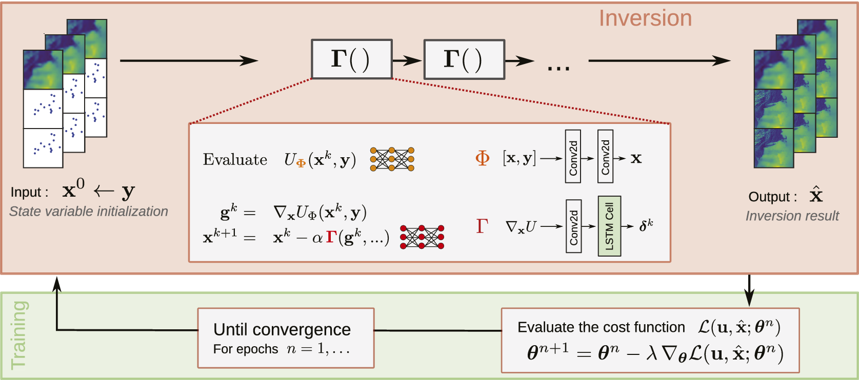
refers to the iteration number. For our experiments, we set the total number of iterations to 5. The 4DVarNet scheme leverages the automatic differentiation capabilities of modern deep learning frameworks to evaluate the gradients of the variational cost (Baydin et al., Reference Baydin, Pearlmutter, Radul and Siskind2018). Figure 2 represents the 4DVarNet scheme graphically, the organization of the input observations and the output reconstructions and the architectures of the trainable networks used. The 4DVarNet can be seen as a bi-level optimization framework to jointly learn the variational model and solver (Fablet and Drumetz, Reference Fablet, Drumetz and Rousseau2020). As the state variable is available from the variational cost minimization, it is used to evaluate a training loss function. This loss function is in turn optimized to fit the trainable networks parameters. These two steps are repeated for the number of training epochs selected by the user.
$ k $
refers to the iteration number. For our experiments, we set the total number of iterations to 5. The 4DVarNet scheme leverages the automatic differentiation capabilities of modern deep learning frameworks to evaluate the gradients of the variational cost (Baydin et al., Reference Baydin, Pearlmutter, Radul and Siskind2018). Figure 2 represents the 4DVarNet scheme graphically, the organization of the input observations and the output reconstructions and the architectures of the trainable networks used. The 4DVarNet can be seen as a bi-level optimization framework to jointly learn the variational model and solver (Fablet and Drumetz, Reference Fablet, Drumetz and Rousseau2020). As the state variable is available from the variational cost minimization, it is used to evaluate a training loss function. This loss function is in turn optimized to fit the trainable networks parameters. These two steps are repeated for the number of training epochs selected by the user.
Schematic illustration of the 4DVarNet framework. The observations and the state variable are prepared as concatenations of the input sources available. The symbol $ \boldsymbol{\theta} $
represents the networks
$ \boldsymbol{\theta} $
represents the networks $ \Phi $
and
$ \Phi $
and $ \Gamma $
parameters and
$ \Gamma $
parameters and $ n $
denotes the training epoch index. The symbol
$ n $
denotes the training epoch index. The symbol $ \mathbf{u} $
represents the ground truths. The statement
$ \mathbf{u} $
represents the ground truths. The statement $ {\mathbf{x}}^0\leftarrow \mathbf{y} $
means that the initial guess of the state variable is initialized with the observations. The red box contains the inversion part to solve for the state variable
$ {\mathbf{x}}^0\leftarrow \mathbf{y} $
means that the initial guess of the state variable is initialized with the observations. The red box contains the inversion part to solve for the state variable $ \mathbf{x} $
, being the parameters
$ \mathbf{x} $
, being the parameters $ \boldsymbol{\theta} $
fixed as of the previous training iteration. The green box highlights the parameters training part to solve for
$ \boldsymbol{\theta} $
fixed as of the previous training iteration. The green box highlights the parameters training part to solve for $ \boldsymbol{\theta} $
, with the state variable
$ \boldsymbol{\theta} $
, with the state variable $ \mathbf{x} $
fixed as returned by the inversion part.
$ \mathbf{x} $
fixed as returned by the inversion part.
The 4DVarNet scheme has been successfully applied to sea-surface height (Beauchamp et al., Reference Beauchamp, Febvre, Georgenthum and Fablet2023), sediment (Vient et al., Reference Vient, Fablet, Jourdin and Delacourt2022), and turbidity (Dorffer et al., Reference Dorffer, Jourdin, Mouillot, Devillers and Fablet2023). The open-source 4DVarNet code base is available on the following repositories, the started version: https://github.com/CIA-Oceanix/4dvarnet-starter and the core version: https://github.com/CIA-Oceanix/4dvarnet-core.
Multimodal version. We mentioned that the problem is inherently multimodal. Both the direct inversion and the 4DVarNet configuration discussed do not process the heterogeneous HR, LR, and local components of the observations $ \mathbf{y} $
separately. We propose the following modification to account explicitly for this input source heterogeneity. The observation term in the variational cost has a further term that evaluates the distance between the feature maps of the observations and the state variable. These feature maps are not constrained by the spatiotemporal characteristics of the observation components and can better relate. The new variational cost reads
$ \mathbf{y} $
separately. We propose the following modification to account explicitly for this input source heterogeneity. The observation term in the variational cost has a further term that evaluates the distance between the feature maps of the observations and the state variable. These feature maps are not constrained by the spatiotemporal characteristics of the observation components and can better relate. The new variational cost reads
 $$ {U}_{\Phi}\left(\mathbf{x},\mathbf{y};\Omega \right)={\lambda}_1\parallel \mathbf{x}-\mathbf{y}{\parallel}_{\Omega}^2+{\lambda}_1\parallel {\psi}_{\mathbf{x}}\left(\mathbf{x}\right)-{\psi}_{\mathbf{y}}\left(\mathbf{y}\right){\parallel}^2+{\lambda}_2\parallel \mathbf{x}-\Phi \left(\mathbf{x}\right){\parallel}^2 $$
where $ {\psi}_{\mathbf{x},\mathbf{y}} $
is the trainable neural networks. For simplicity, we call single-modal the 4DVarNet based on the plain variational cost 3 and we call multimodal the 4DVarNet based on the variational cost 6. In both the single and multimodal versions of the 4DVarNet, we choose to train the weights
$ {\psi}_{\mathbf{x},\mathbf{y}} $
is the trainable neural networks. For simplicity, we call single-modal the 4DVarNet based on the plain variational cost 3 and we call multimodal the 4DVarNet based on the variational cost 6. In both the single and multimodal versions of the 4DVarNet, we choose to train the weights $ {\lambda}_{1,2} $
as well.
$ {\lambda}_{1,2} $
as well.
3.3. Numerical implementation
The observations and state variable objects are obtained by concatenating the LR and anomaly fields, see Figure 2. The anomaly is the difference between the HR and LR fields. The LR represents the average field information, while the anomaly is the deviation from the LR of the HR field. This choice prevents the model to process redundantly the LR information. We choose a 2D convolutional neural network to parameterize both for the direct inversion and the dynamical prior $ \Phi $
of the 4DVarNet. The gradient solver
$ \Phi $
of the 4DVarNet. The gradient solver $ \Gamma $
is parameterized by a 2D convolutional LSTM (Hochreiter and Schmidhuber, Reference Hochreiter and Schmidhuber1997). The networks
$ \Gamma $
is parameterized by a 2D convolutional LSTM (Hochreiter and Schmidhuber, Reference Hochreiter and Schmidhuber1997). The networks $ {\psi}_{\mathbf{x},\mathbf{y}} $
are composed by 2D or 1D convolutional layers depending on the experimental configuration. Recall that by configuration we mean the input data combinations. 2D layers process spatial image fields and 1D layers are well suited for multivariate time series.
$ {\psi}_{\mathbf{x},\mathbf{y}} $
are composed by 2D or 1D convolutional layers depending on the experimental configuration. Recall that by configuration we mean the input data combinations. 2D layers process spatial image fields and 1D layers are well suited for multivariate time series.
3.4. Learning scheme
The models are trained with the following supervised mean-squared-error cost function:
 $$ {\displaystyle \begin{array}{l}\mathrm{\mathcal{L}}\left(\mathbf{u},\hat{\mathbf{x}}\right)=\frac{1}{M}\sum \limits_{i=0}^M\sum \limits_{t=0}^T\hskip0.1em {\lambda}_l\parallel {\mathbf{u}}_{it}^{lr}-{\hat{\mathbf{x}}}_{it}^{lr}{\parallel}^2+{\lambda}_h\parallel {\mathbf{u}}_{it}^{hr}-{\hat{\mathbf{x}}}_{it}^{hr}{\parallel}^2+\hskip3em \\ {}\hskip6.560001em +{\lambda}_g\parallel \nabla {\mathbf{u}}_{it}^{hr}-\nabla {\hat{\mathbf{x}}}_{it}^{hr}{\parallel}^2+{\lambda}_p\parallel {\hat{\mathbf{x}}}_{it}^{hr}-\Phi \left({\hat{\mathbf{x}}}_{it}^{hr}\right){\parallel}^2\end{array}} $$
Let $ \mathbf{u} $
and
$ \mathbf{u} $
and $ \hat{\mathbf{x}} $
be the ground truths and the reconstructions, respectively. The symbols
$ \hat{\mathbf{x}} $
be the ground truths and the reconstructions, respectively. The symbols $ M $
and
$ M $
and $ T $
represent the number of elements in each data batch and the time window length, that is, 24 hours. To evaluate the loss function, we obtain the HR fields summing the LR and anomaly components of the reconstructed state variable. The spatial gradients term enforces the spatial coherence of the output fields. These gradients, evaluated with the finite difference method available in the Pytorch library, are computed with respect to the coordinates that define the fields spatial grid. Note that these spatial finite difference-based gradients are evaluated numerically. This has nothing in common with the gradients of the variational cost, as in the first line of Equation 5, which are evaluated by automatic differentiation. The last training loss term acts as a regularization and enforces the parameters to be learned in compliance with the dynamics specified by the first equation of the state-space formulation 1. This term should not be dominant, so the weight
$ T $
represent the number of elements in each data batch and the time window length, that is, 24 hours. To evaluate the loss function, we obtain the HR fields summing the LR and anomaly components of the reconstructed state variable. The spatial gradients term enforces the spatial coherence of the output fields. These gradients, evaluated with the finite difference method available in the Pytorch library, are computed with respect to the coordinates that define the fields spatial grid. Note that these spatial finite difference-based gradients are evaluated numerically. This has nothing in common with the gradients of the variational cost, as in the first line of Equation 5, which are evaluated by automatic differentiation. The last training loss term acts as a regularization and enforces the parameters to be learned in compliance with the dynamics specified by the first equation of the state-space formulation 1. This term should not be dominant, so the weight $ {\lambda}_p $
is set to a small value. In this case,
$ {\lambda}_p $
is set to a small value. In this case, $ {\lambda}_p={10}^{-3} $
. We train the model for 50 epochs with the Adam algorithm (Kingma and Ba, Reference Kingma and Ba2014). Training is regularized by the
$ {\lambda}_p={10}^{-3} $
. We train the model for 50 epochs with the Adam algorithm (Kingma and Ba, Reference Kingma and Ba2014). Training is regularized by the $ {L}_2 $
method and by early stopping based on the validation loss.
$ {L}_2 $
method and by early stopping based on the validation loss.
The learning rates for $ \Phi $
,
$ \Phi $
, $ \Gamma $
, and the parameters
$ \Gamma $
, and the parameters $ {\lambda}_{1,2} $
are, respectively,
$ {\lambda}_{1,2} $
are, respectively, $ {10}^{-4} $
,
$ {10}^{-4} $
, $ {10}^{-3} $
, and
$ {10}^{-3} $
, and $ {10}^{-4} $
. The weight decay coefficients are, in the same order,
$ {10}^{-4} $
. The weight decay coefficients are, in the same order, $ {10}^{-5} $
,
$ {10}^{-5} $
, $ {10}^{-5} $
, and
$ {10}^{-5} $
, and $ {10}^{-8} $
. The coefficients
$ {10}^{-8} $
. The coefficients $ {\lambda}_l $
,
$ {\lambda}_l $
, $ {\lambda}_h $
, and
$ {\lambda}_h $
, and $ {\lambda}_g $
are, respectively,
$ {\lambda}_g $
are, respectively, $ 2.5 $
,
$ 2.5 $
, $ 15 $
, and
$ 15 $
, and $ {10}^{-2} $
. In the multimodal 4DVarNet case, the models
$ {10}^{-2} $
. In the multimodal 4DVarNet case, the models $ {\psi}_{\mathbf{x},\mathbf{y}} $
have learning rate and weight decay coefficient set to
$ {\psi}_{\mathbf{x},\mathbf{y}} $
have learning rate and weight decay coefficient set to $ {10}^{-4} $
and
$ {10}^{-4} $
and $ {10}^{-7} $
. We used a batch size
$ {10}^{-7} $
. We used a batch size $ 8 $
for all the simulationsFootnote
2.
$ 8 $
for all the simulationsFootnote
2.
4. Results
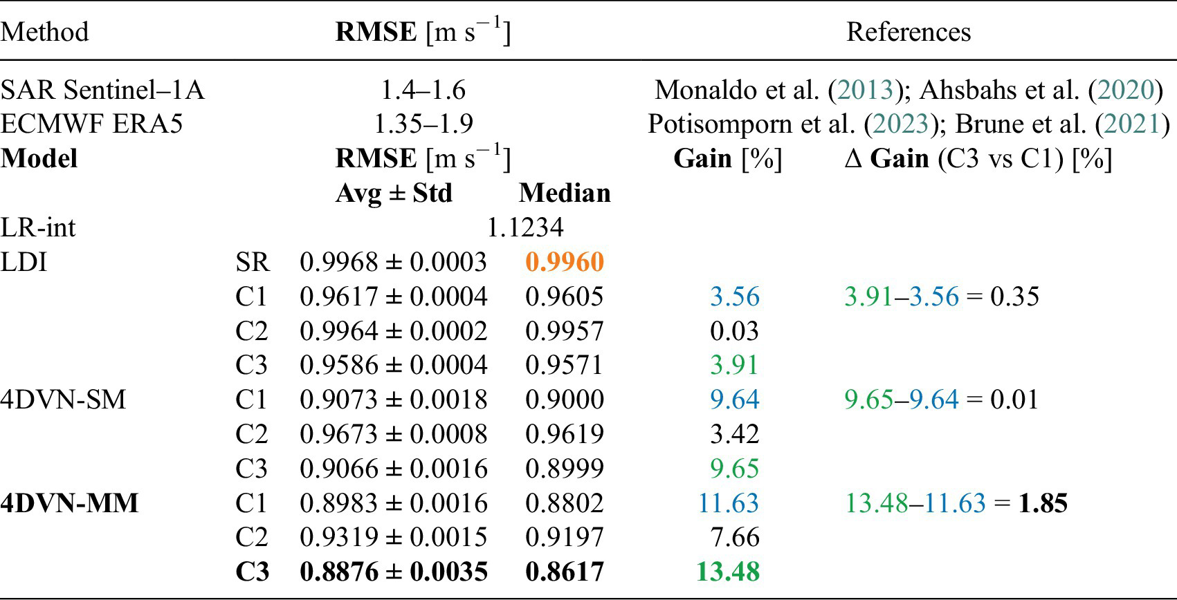
In the presentation of the results, we adopt the following notation. Let LDI be the direct inversion baseline. Let 4DVN-SM denote the single-modal 4DVarNet version and 4DVN-MM the multimodal version. Let the symbols {LDI, 4DVN-SM, 4DVN-MM}-{SR, C[1,2,3]} indicate the model-data configuration combinations. These abbreviations are, for readers’ convenience, restated systematically in part A of Table 1. The target of each model are the ground truth HR original fields.
Global overview on the benchmark experiments
Table A—Table of the abbreviations used in the results presentation. The symbol ✘ states that a given input data source is missing. 1 h, 6 h, and 12 h stand, respectively, for observation sampling frequency of 1, 6, and 12 h.

—Benchmark test results. To contextualize our results, the first two rows report the typical reconstruction errors expected when using SAR Sentinel-1A imagery and the wind speed reanalyses of the ECMWF ERA-5 catalog. In the second part of this Table, we report the RMSE scores for our simulations, expressed by Equations 8 and 9. Relative gains are expressed in percentage. The gains are referred to the LDI-SR baseline, marked in orange. The black boldface highlights the best result. We follow the names conventions stated in part A of this Table.
4.1. Evaluation framework
To set up the evaluation scheme, we chose a proper reference metric for the sea-surface wind speed reconstruction. In the literature, reference values for the root-mean-squared error (RMSE) can be found for SAR-derived wind speed fields (Monaldo et al., Reference Monaldo, Jackson and Pichel2013; Ahsbahs et al., Reference Ahsbahs, Maclaurin, Draxl, Jackson, Monaldo and Badger2020) and reanalyzed products (Brune et al., Reference Brune, Keller and Wahl2021; Gualtieri, Reference Gualtieri2021; Potisomporn et al., Reference Potisomporn, Adcock and Vogel2023). Part B of Table 1 reports the reference values provided by the cited work. The RMSE score is evaluated for SAR and reanalyses using in situ observations and assuming that these observations match the true wind values. In our case, we use synthetic simulated data and we have no in situ observations to be used as ground truth.Footnote 3 To fix a reference performance value, we do the following. We interpolate the LR fields in time on the 24-hour window. Recall that our experimental configurations have LR fields with observation frequency of 6 hours. We then evaluate the RMSE between these interpolated time series and the ground truth HR fields. Let B-RMSE represent this metric, which attains the value of 1.1234 m s−1. We assume that our HR ground truth fields match the real physical phenomenon. In this way, we can directly compare our B-RMSE with the RMSE range found in the literature for reanalyzed fields, that is, 1.35–1.9 m s−1. Our B-RMSE attains a lower value than the lower bound of this interval. This is due to the fact that our interpolated LR fields, simulating real reanalyses, are not affected by model errors, as happens for real reanalyses. In this way, we can fix our B-RMSE as a quantitative reference for this case study. That is, if only LR NWP products were available. Next, we evaluate how two classes of trainable models (direct inversion and 4DVarNet) give better reconstruction performance leveraging (i) learnable modules and/or (ii) heterogeneous input observations. We may emphasize that we choose as baseline the superresolution direct inversion model LDI-SR because it is the simplest method that aims to reconstruct the HR ground truth fields, while the LR interpolation approach does not. Therefore, we keep the mentioned B-RMSE as quantitative reference, but it would not be a fair baseline to assess the 4DVarNet performance improvement.
The reconstructions of our models are evaluated with the RMSE score related to an ensemble of 10 model runs. We assess the RMSE in two ways. First, we collect the reconstruction RMSEs between each model’s output and the ground truths. We evaluate the average RMSE and the standard deviation as measures of centrality and spread. In formulas
 $$ {\displaystyle \begin{array}{c}\mathrm{Avg}\;\mathrm{RMSE}\left(\hat{\mathbf{x}},\mathbf{u}\right)=\frac{1}{R}{\sum}_{r=1}^R\mathrm{RMSE}\left({\hat{\mathbf{x}}}_r,\mathbf{u}\right)=\frac{1}{R}{\sum}_{r=1}^R\sqrt{\frac{1}{M}{\sum}_{i=1}^M{\left({\hat{\mathbf{x}}}_r-\mathbf{u}\right)}^2}\\ {}\mathrm{Std}\;\mathrm{RMSE}\left(\hat{\mathbf{x}},\mathbf{u}\right)=\sqrt{\frac{1}{R}{\sum}_{r=1}^R{\left(\mathrm{AvgRMSE}-\mathrm{RMSE}\left(\hat{\mathbf{x}},\mathbf{u}\right)\right)}^2}\end{array}} $$
where $ \mathbf{u} $
is the ground truth,
$ \mathbf{u} $
is the ground truth, $ {\hat{\mathbf{x}}}_r $
is the model
$ {\hat{\mathbf{x}}}_r $
is the model $ r $
reconstruction,
$ r $
reconstruction, $ R $
is the number of model runs, equivalent to the ensemble members, and
$ R $
is the number of model runs, equivalent to the ensemble members, and $ M $
is the number of samples. Second, the RMSE is evaluated between the ground truths and the median of an ensemble of 10 model runs (Rincy and Gupta, Reference Rincy and Gupta2020). In formulas
$ M $
is the number of samples. Second, the RMSE is evaluated between the ground truths and the median of an ensemble of 10 model runs (Rincy and Gupta, Reference Rincy and Gupta2020). In formulas
 $$ \mathrm{M}\mathrm{e}\mathrm{d}\mathrm{i}\mathrm{a}\mathrm{n}\ \mathrm{R}\mathrm{M}\mathrm{S}\mathrm{E}(\hat{\mathbf{x}},\mathbf{u})=\mathrm{R}\mathrm{M}\mathrm{S}\mathrm{E}(\mathbf{u},\mathrm{M}\mathrm{e}\mathrm{d}\mathrm{i}\mathrm{a}\mathrm{n}(\{{\hat{\mathbf{x}}}_r;r=1,\dots, R\})) $$
We define a relative gain to compare the model improvement w.r.t. the chosen baseline as $ \left(1-{p}_m/{p}_b\right)\times 100 $
, where
$ \left(1-{p}_m/{p}_b\right)\times 100 $
, where $ {p}_m $
and
$ {p}_m $
and $ {p}_b $
are the performance of the model and baseline, respectively.
$ {p}_b $
are the performance of the model and baseline, respectively.
4.2. Model benchmark
The 4DVarNet is compared against the LDI-SR model. This baseline model is trained to perform a superresolution task to retrieve the finer-scaled information from the LR input fields. The neural network used for the direct learning–based inversion shares the same architecture used to parameterize the dynamical prior $ \Phi $
of the 4DVarNet framework. Part B of Table 1 lists systematically the simulations results. We can see that the 4DVarNet, in both the single and multimodal versions, outperforms the direct inversion baseline. However, the 4DVN-SM model does not benefit fully from the in situ observations, and indeed, the baseline does. The rightmost column of the table evaluates the difference between the performance associated to the configuration C3 w.r.t. the configuration C1. That is, the added value of in situ time series. In the case of 4DVN-MM, thanks to the features maps term in the variational cost 6, the framework can effectively benefit from the in situ time series. Figure 3 illustrates the spatial distribution of the time-average gain of the C3 configuration w.r.t. the C1 configuration, for both the 4DVN-SM and 4DVN-MM models. The single-modal 4DVN-SM, despite outperforming the direct inversion baseline, does not fully use the HR information of the satellite pseudo-observations. 4DVN-MM, on the other hand, can effectively extract the spatiotemporal HR information from both satellite pseudoproducts and in situ time series. The effect of this multimodal skill is reflected in the area affected by the reconstruction improvement, on tens-of-kilometers neighborhoods of the in situ buoys.
$ \Phi $
of the 4DVarNet framework. Part B of Table 1 lists systematically the simulations results. We can see that the 4DVarNet, in both the single and multimodal versions, outperforms the direct inversion baseline. However, the 4DVN-SM model does not benefit fully from the in situ observations, and indeed, the baseline does. The rightmost column of the table evaluates the difference between the performance associated to the configuration C3 w.r.t. the configuration C1. That is, the added value of in situ time series. In the case of 4DVN-MM, thanks to the features maps term in the variational cost 6, the framework can effectively benefit from the in situ time series. Figure 3 illustrates the spatial distribution of the time-average gain of the C3 configuration w.r.t. the C1 configuration, for both the 4DVN-SM and 4DVN-MM models. The single-modal 4DVN-SM, despite outperforming the direct inversion baseline, does not fully use the HR information of the satellite pseudo-observations. 4DVN-MM, on the other hand, can effectively extract the spatiotemporal HR information from both satellite pseudoproducts and in situ time series. The effect of this multimodal skill is reflected in the area affected by the reconstruction improvement, on tens-of-kilometers neighborhoods of the in situ buoys.
Average gains maps. Left panel: plain 4DVarNet, average gain of 4DVN-SM-C3 vs 4DVN-SM-C1. Right panel: 4DVarNet with the additive trainable observation term in the variational cost, 4DVN-MM-C3 vs 4DVN-MM-C1.

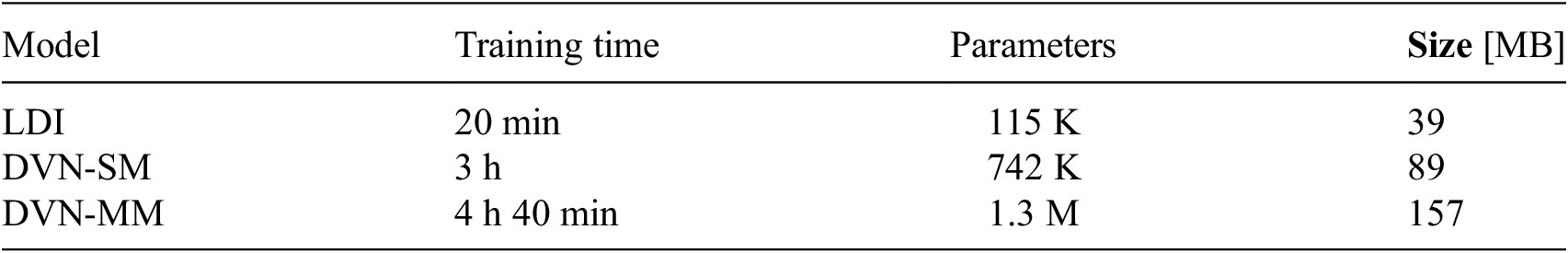
To complete the systematic benchmark of our models, we show in Table 2 that the computational effort associated with each model is used. We report the training time for the ensemble of 10 model runs, the trainable parameters of one single model of the ensemble, and the memory size required to store the 10-member model ensemble. Not surprisingly, the multimodal 4DVarNet 4DVN-MM is the most expensive model in terms of resources.
Computational effort associated to the models used. Training times refer to the time required to train the ensemble of 10 models. The trainable parameters are the number of parameters of one single model. Memory size refers to the space required to save the 10-members model ensemble
4.3. Biased LR data
Reanalyzed NWP products can be biased by model errors. To emulate this scenario, we train our models on an artificially biased dataset where the LR fields are modified by a random delay of $ \left[-4,+4\right] $
hours or a random phase amplitude of
$ \left[-4,+4\right] $
hours or a random phase amplitude of $ \left[\mathrm{0.5,1.5}\right] $
. Formally,
$ \left[\mathrm{0.5,1.5}\right] $
. Formally,
 $$ {\mathbf{y}}^{lr}(t)=\left\{\begin{array}{l}{\mathbf{y}}^{lr}\left(t+\Delta t\right)\;\mathrm{with}\;\Delta t\hskip0.22em \sim \hskip0.22em \mathcal{U}\left(-4,+4\right)\\ {}\hskip1.12em \alpha \hskip0.1em {\mathbf{y}}^{lr}(t)\;\mathrm{with}\;\alpha \hskip0.22em \sim \hskip0.22em \mathcal{U}\left(\mathrm{0.5,1.5}\right)\end{array}\right. $$
where $ \mathcal{U} $
represents the uniform distribution. Interestingly, this at-train-time modification can be seen as a dynamic data augmentation process (Xu et al., Reference Xu, Lee and Hsu2021). At test time, the model is evaluated using a test set that is systematically modified by each one of the modification factors. In this way, we can visualize a set of performance curves that depict that reconstruction error as a function of the modification factor, see Figure 4. In the case of random delay, the reconstruction curves for 4DVN-MM-C3 are lower at the extremes. This means that the model trained on the biased dataset learns the error in LR fields. Intriguingly, the curve associated with 4DVN-MM-C3 is systematically lower than the curve of 4DVN-SM-C3. This proves that the modeling choice of the additional term in the variational cost 6 gives the model the capability to learn and generalize even in the case of biased input data. In the amplitude case, the effect is less pronounced. An explanation of this phenomenon could be the following. In the delay case, there is a clear mismatch between the HR field and the swapped LR field. The LR field remodulation by the amplitude factors we chose may not suffice to make the field drastically different from the original. This implies a lesser model capability to detect and attenuate the LR data bias.
$ \mathcal{U} $
represents the uniform distribution. Interestingly, this at-train-time modification can be seen as a dynamic data augmentation process (Xu et al., Reference Xu, Lee and Hsu2021). At test time, the model is evaluated using a test set that is systematically modified by each one of the modification factors. In this way, we can visualize a set of performance curves that depict that reconstruction error as a function of the modification factor, see Figure 4. In the case of random delay, the reconstruction curves for 4DVN-MM-C3 are lower at the extremes. This means that the model trained on the biased dataset learns the error in LR fields. Intriguingly, the curve associated with 4DVN-MM-C3 is systematically lower than the curve of 4DVN-SM-C3. This proves that the modeling choice of the additional term in the variational cost 6 gives the model the capability to learn and generalize even in the case of biased input data. In the amplitude case, the effect is less pronounced. An explanation of this phenomenon could be the following. In the delay case, there is a clear mismatch between the HR field and the swapped LR field. The LR field remodulation by the amplitude factors we chose may not suffice to make the field drastically different from the original. This implies a lesser model capability to detect and attenuate the LR data bias.
Biased LR field tests. Left panel: random delay. Right panel: random intensity. The suffixes “-rd” and “-ri” identify the models trained in the case of random delay and intensity, respectively.

5. Conclusions
Our analysis presents the application of a hybrid data assimilation and deep learning framework used to retrieve HR wind speed fields from the partial observations of sea-surface wind. We showed that this framework can outperform a deep learning–based direct inversion scheme. We see that the 4DVarNet scheme improves the baseline in two independent ways. The first is imputable to the underlying 4DVar formulation that accounts explicitly for time processes. This informs the reconstruction of the temporal features of the phenomenon. On the other hand, the 4DVN-MM model better exploits the different input sources. This multimodal skill covers a primary importance in oceanography and geosciences since the large volumes of Earth observations are characterized by different spatiotemporal features. Our results show that proper modeling choices allow us to profit from the complementary information conveyed by these diverse observation sources. We also proved that these modeling choices, thanks to the flexibility of deep learning modeling, can endow the 4DVarNet framework with improved generalization capabilities that help to attenuate the errors in NWP products.
Open peer review
To view the open peer review materials for this article, please visit http://doi.org/10.1017/eds.2024.34.
Acknowledgments
The computing resources were provided by the Région Bretagne, via the project CPER AIDA (2021–2027).
Author contribution
Conceptualization: M.Z; N.F; D.C; A.G; R.F. Methodology: N.F; D.C; R.F. Data curation: M.Z. Data visualization: M.Z. Writing original draft: M.Z; N.F; D.C; A.G; R.F. All authors approved the final submitted draft.
Data availability statement
The source code used for the simulations is available at https://github.com/CIA-Oceanix/4DVN-MM-W2D. RUWRF data are available through the THREDDS Data Server at https://tds.marine.rutgers.edu/thredds/cool/ruwrf/catalog.html.
Provenance statement
This article is part of the Climate Informatics 2024 proceedings and was accepted in Environmental Data Science on the basis of the Climate Informatics peer review process.
Funding statement
This research was supported by grants from the ANR Chair Oceanix ANR-19-CHIA-0016; Agence Nationale de la Recherche (ANR). The work has been co-funded by Naval Group.
Competing interest
None.
Ethical standard
The research meets all ethical guidelines, including adherence to the legal requirements of the study country.


 Open access
Comments
Dr. Claire Monteleoni,
Editor-in-Chief
Environmental Data Science
Dear Dr. Monteleoni,
This letter supports the submission of our paper “Multi-Modal
Learning-based Reconstruction of High-Resolution Spatial
Wind Speed Fields” to Environmental Data Science.
Our work addresses the joint exploitation of ocean
remote sensing and in-situ observations in sea surface
state data-driven modeling. We focus in particular on
sea surface wind speed. We propose a hybrid deep learning
and variational data assimilation framework to simultaneously
process heterogeneous and multi-sensor sources of information.
The originality of this work stems from the effectiveness of our
proposed framework to exploit the complementary information
conveyed by the input data. The numerical experiments and the
results detailed in our paper show that our model is competitive
with the baseline provided by the performance level of Numerical
Weather Forecast models, as ECMWF ERA-5 and purely
learning-based schemes.
We think that this work may be of interest for operational applications,
ocean engineering practitioners as well as for researchers in the
field of data-driven ocean surface modeling, particularly on the
topic of multi-modal learning and multi-sensor information
processing and fusion.
The correspondence should be addressed to Matteo Zambra
at matteo.zambra1@gmail.com and to Prof. Ronan Fablet
at ronan.fablet@imt-atlantique.fr.
Thank you for your attention and consideration.
Kindest regards,
Matteo Zambra
Ph.D.
IMT Atlantique, UMR CNRS Lab-STICC
Brest, France
(Previous affiliation)
matteo.zambra1@gmail.com
Ronan Fablet
Full Professor
IMT Atlantique, UMR CNRS Lab-STICC
Brest, France
ronan.fablet@imt-atlantique.fr