


1. Introduction
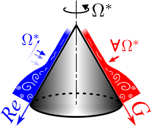
The three-dimensional boundary layer induced by a cone rotating in otherwise still fluid has been studied where the flow geometry is defined by the half-apex angle  $\psi$ (figure 1). We consider an orthogonal coordinate system with the origin located at the apex of the cone shown in figure 1, where $x$,
$x$,  $\theta$ and $z$ are the coordinates along the generatrix of the cone, azimuthal and wall-normal directions, respectively. Lengths are normalised by $\delta _{\nu }^{*}=\sqrt {\nu ^{*}/ (\varOmega ^{*}\sin \psi )}$, where $\nu ^{*}$ and $\varOmega ^{*}$ are the kinematic viscosity of the surrounding fluid and angular velocity, respectively (superscript $^{*}$ denotes a dimensional quantity). Note that the commonly used Reynolds number based on $x^{*}$ and the local wall velocity $V_{w}^{*}$ is the square of $x=x^*/\delta _{\nu }^{*}$. Scaling the lengths with $\delta _{\nu }^{*}$, one obtains the same von Kármán similarity solution as for the rotating disk for the mean flow on the cone (Segalini & Camarri Reference Segalini and Camarri2019). The flow visualisations conducted by Kobayashi & Izumi (Reference Kobayashi and Izumi1983) show that depending on $\psi$ the flow is dominated by different instabilities; on a broad cone (including the disk, i.e. $\psi =90^{\circ }$) cross-flow instability develops and is observed as stationary co-rotating vortices similar to the ones on a swept wing. On sharper cones ( $\psi \lesssim 40^{\circ }$), in contrast, centrifugal instability becomes dominant (including the cylinder, i.e. $\psi =0^{\circ }$), giving rise to counter-rotating vortices. Recent works provide further quantitative data for broad cones (Imayama, Alfredsson & Lingwood Reference Imayama, Alfredsson and Lingwood2012, Reference Imayama, Alfredsson and Lingwood2013, Reference Imayama, Alfredsson and Lingwood2014; Kato, Alfredsson & Lingwood Reference Kato, Alfredsson and Lingwood2019a; Kato et al. Reference Kato, Kawata, Alfredsson and Lingwood2019b). However, such detailed experimental data on slender cones have up to now not been available.
The coordinate system  $(x, \theta , z)$ on the cone and its dimension.

A crucial question for the slender rotating-cone flow is the effect of the rotational rate  $\varOmega ^{*}$ on transition. The reported transition locations and the influence of $\varOmega ^{*}$ are highly variable on the slender cones while independent works on the disk show more consistent results (see Imayama et al. (Reference Imayama, Alfredsson and Lingwood2013), and the references therein); Kreith, Ellis & Giesing (Reference Kreith, Ellis and Giesing1963, figure 5), Kobayashi & Izumi (Reference Kobayashi and Izumi1983, § 3.3) and Tieng & Wang (Reference Tieng and Wang1993, figure 9) reported that $\varOmega ^{*}$ does not affect the transition Reynolds number significantly. In contrast, Hussain, Garrett & Stephen (Reference Hussain, Garrett and Stephen2014, figure 2 made by Nickels and Betényi originally) show that the transition Reynolds number decreases as $\varOmega ^{*}$ increases with a trend that becomes more significant as $\psi$ decreases.
In this paper, we evaluate the flow on a slender cone ( $\psi = 30^{\circ }$) at different rotational rates based on a Görtler number $G$ (in addition to $x$), which has been used for flows dominated by centrifugal instability, e.g. the boundary layer on a concave wall (Floryan Reference Floryan1986; Schrader, Brandt & Zaki Reference Schrader, Brandt and Zaki2011; Méndez et al. Reference Méndez, Shadloo, Hadjadj and Ducoin2018). For such boundary-layer flows, the free-stream velocity is used as the reference velocity; however, here we define the Görtler number for the rotating-cone boundary layer as
 \begin{equation} G=\frac{V_{w}^{*} \delta_{2}^{*}}{\nu^{*}}\sqrt{\frac{\delta_{2}^{*}}{R^{*}}}=\sqrt{\frac{x \,\delta_{2}^{3}}{\sin \psi}}, \end{equation}
where the reference velocity is the local wall velocity  $V_{w}^{*}=R^{*}\varOmega ^{*}$, the radius is $R^{*}=x^{*} \sin \psi$, which is considered as the curvature of the streamline on the surface, and $\delta _{2}$ is the momentum thickness normalised by $\delta ^{*}_{\nu }$. The momentum thickness is evaluated as
 \begin{equation} \delta_{2}(x; \varOmega^{*})=\int_{0}^{ \delta_{90}} [1-V(x, z; \varOmega^{*})]V(x, z; \varOmega^{*})\, \mathrm{d} z, \end{equation}
where  $V$ is the measured mean azimuthal velocity component normalised by $V_{w}^{*}$ and $\delta _{90}$ is the $z$-position (normalised by $\delta ^{*}_{\nu }$) where $V$ is 0.1. Also, we compare the results with local linear stability analysis (LLSA) as a complement to the present experiments.
2. LLSA
The LLSA is performed similarly to the analysis of Segalini & Camarri (Reference Segalini and Camarri2019). The linear perturbation equations in the laboratory frame of reference are solved in a parallel framework at several  $x$-locations, where at each station the local mean velocity profile from the von Kármán profile is imposed (here denoted as $U_0(z)$, $V_0(z)$ and $W_0(z)$ for $x$-,
$x$-,  $\theta$- and $z$-components, respectively, with $V_0(z=0)=1$ according to the adopted normalisation). Time is normalised by $\varOmega ^*$, and the base and perturbation velocity fields are normalised by $(\nu ^*\varOmega ^*\sin \psi )^{1/2}$.
Modal analysis of the velocity components and pressure in the form  $(u, v, w, p)\propto (\hat{u}, \hat{v}, \hat{w}, \hat{p})(z)\exp [\mathrm {i}(\alpha x+n\theta -\omega t)]$ is performed to transform the perturbation equations to a set of ordinary differential equations with the eigenfunctions and eigenvalue $\alpha =\alpha _{r}+{\mathrm i} \alpha _{i}$ as unknowns. This eigenvalue problem was solved at several $x$-locations to account for the change of the base velocity profile. Here $n$ and $\omega$ are the azimuthal wavenumber (taking only integer values due to the continuity in $\theta$-direction) and frequency (the latter normalised by $\varOmega ^{*}$), respectively. Due to the small boundary-layer thickness, the radial variation in the $z$-direction is assumed constant ( $r\approx x\sin \psi$ within the boundary layer). Differently from Segalini & Camarri (Reference Segalini and Camarri2019), terms of order $O(x)^{-2}$ have been discarded in the analysis without significant deviations from the full parallel and weakly divergent solution. The perturbation equations in modal form are
 \begin{gather} \left(\mathrm{i}\alpha+\frac{1}{x}\right)\hat{u} + \textrm{i}\beta\hat{v} + \frac{\partial \hat{w}}{\partial z}+\frac{1}{x}\cot\psi\hat{w}=0, \end{gather}
 \begin{gather}\left[\mathcal{L}+{U}_0\right]\hat{u}-2V_0\hat{v}+ x\frac{\mathrm{d}{U_0}}{\mathrm{d} z}\hat{w} + \mathrm{i}\alpha\hat{p}=0, \end{gather}
 \begin{gather}2V_0\hat{u}+\left[\mathcal{L}+{U}_0\right]\hat{v}+x\frac{\mathrm{d}{V_0}}{\mathrm{d} z}\hat{w}+\cot\psi{V}_0\hat{w} +\mathrm{i}\beta\hat{p}=0, \end{gather}
 \begin{gather}-2\cot\psi{V}_0\hat{v}+\left[\mathcal{L}+\frac{\mathrm{d}{W}_{0}}{\mathrm{d} z}\right]\hat{w}+\frac{\partial \hat{p}}{\partial z} =0, \end{gather}
with the linear operator
 \begin{align} \mathcal{L}={-}\frac{\mathrm{i}\omega}{\sin\psi} +\mathrm{i}\alpha x{U}_0+\mathrm{i}\beta x{V}_0+W_0\frac{\partial}{\partial z}+\alpha^2+\beta^2-\frac{\partial^2}{\partial z^2}-\frac1{x}\left(\mathrm{i}\alpha+\cot\psi\frac{\partial}{\partial z}\right), \end{align}
with  $\beta =n/(x\sin \psi )$. A Chebyshev collocation method with 100 points was used to solve (2.1)–(2.4). The points followed an exponentially mapped Gauss–Lobatto distribution within a domain between the wall and the upper boundary located at $z_{max}=40$.
3. Experiment
A solid aluminium-alloy cone was mounted on an air bearing and rotated by a DC motor as shown in figure 1. It has a smooth surface (surface roughness of approximately  $1\ \mathrm {\mu } \textrm {{m}}$) and the rotational imbalance was approximately $10\ \mathrm {\mu }\textrm {{m}}$ at the cone edge. The azimuthal velocity component in the laboratory frame of reference ( $V+v$, where $v$ is the variation in time) was measured by a single hot-wire probe (its diameter was $2.5\ \mathrm {\mu }\textrm {m}$ and the sensing length approximately 0.7 mm) at fixed points in the laboratory frame of reference and normalised by $V_{w}^{*}$. In contrast to the periodic signal due to cross-flow vortices on broad cones (Imayama et al. Reference Imayama, Alfredsson and Lingwood2014; Kato et al. Reference Kato, Kawata, Alfredsson and Lingwood2019b), preliminary tests showed that the signal contains multiple wave packets, which appear spontaneously rather than periodically and seem to be similar to noise-sustained structures on a rotating cylinder exposed to an axial flow due to a convective instability (Babcock, Ahlers & Cannell Reference Babcock, Ahlers and Cannell1991; Tsameret & Steinberg Reference Tsameret and Steinberg1994). To obtain accurate statistics of the irregular waves, the signal was recorded for 3600 cone revolutions. The stationary component with respect to the cone surface was evaluated by phase averaging (according to the cone revolution) the whole length of the sample record. The non-stationary component was obtained by subtracting the spectrum of the stationary modes from the total one in the same way as was done by Kato et al. (Reference Kato, Segalini, Alfredsson and Lingwood2019c).
4. Results and discussions
Figure 2 shows the measured 90 % boundary-layer thickness  $\delta _{90}$ as function of $x$ and $G$ for the different rotation rates. In the laminar region, $\delta _{90}$ is nearly constant following the similarity solution, which is shown by the solid line $\delta _{90}=2.81$ (except a slight overshoot at $x=150$). For each case, the boundary layer thickens as $x$ and $G$ increase, indicating the onset of transition. The transition begins at smaller $x$ as $\varOmega ^{*}$ increases as shown in figure 2(a) whereas figure 2(b) shows that all data collapse nicely on a single curve. Furthermore, the thickening starts in the range $8 \lesssim G \lesssim 10$. The value of $G=10$ is also marked by the arrows in figure 2(a). Beyond $G\approx 10$, the thickness increases with a slope of 2/3, indicating that $\delta _{2}$ is proportional to $\delta _{90}$ (see (1.1)). (The data can be found in tables as supplementary material available at https://doi.org/10.1017/jfm.2021.216.) It is also interesting that this threshold of $G$ is close to the one where the boundary layer on a concave wall starts to transition under low turbulence condition (Liepmann Reference Liepmann1945).
Normalised 90 % boundary-layer thickness  $\delta _{90}$ as a function of (a) $x$ and (b) Görtler number $G$. The thick line $\delta _{90}=2.81$ shows the similarity solution. The arrows at the abscissa in panel (a) indicate the transition Görtler number $G=$10. The insert in panel (b) expands the region where the transition starts.

Figure 3 shows a typical development of the mean velocity and r.m.s. profiles (ai–x) and probability density function (p.d.f.) normalised by the local maximum (bi–x). In the laminar region, the mean profiles agree with the similarity solution (solid line). Beyond  $G\approx 10$ (aiii,biii), the 90 % boundary-layer thickness (dotted line) starts to increase and the profile begins to deviate from the similarity solution. The p.d.f. initially develops symmetrically (bi), and then begins to skew. Following the discussions by Kato et al. (Reference Kato, Kawata, Alfredsson and Lingwood2019b), the skewed profiles in (bii–iv) probably indicate the downwelling of low-momentum fluid at low $z$ and upwelling of high-momentum fluid at high $z$ although here the vortices are counter-rotating and not stationary with respect to the cone surface as the co-rotating stationary cross-flow vortices are. In (bv–vii), the branched maximum is also observed for $z>2$, which may indicate the overturning of the upwelling high-momentum fluid extending to the outer region of the boundary layer. Finally, the similarity of p.d.f. profiles in (bviii–x) indicates that the boundary layer has reached a turbulent state.
Profiles of azimuthal mean velocity  $V$ (in the laboratory frame) and r.m.s. of the azimuthal velocity fluctuation $v$ (
$v$ ( ${\bigcirc}$ and $\times$, (a i–x)) and p.d.f. of $v$ (b i–x) at different $x$-locations ( $\varOmega ^{*}=900$ rpm): (a i,b i) $x = 200$ ( $G=7.9$), (a ii,b ii) $x = 260$ ( $G=9.9$), (a iii,b iii) $x = 280$ ( $G=10.1$), (a iv,b iv) $x = 300$ ( $G=12.1$), (a v,b v) $x = 320$ ( $G=14.9$), (a vi,b vi) $x = 340$ ( $G=21.8$), (a vii,b vii) $x = 360$ ( $G=34.3$), (a viii,b viii) $x = 380$ ( $G=46.9$), (a ix,b ix) $x = 400$ ( $G=57.6$), (a x,b x) $x = 440$ ( $G=71.1$). The solid lines in panels (a i–x) show the similarity solution. The thick horizontal dashed lines indicate the measured 90 % boundary-layer thickness $\delta _{90}$.

Figure 4 shows the p.d.f. of  $v$ at $z=1.5$ as a function of downstream position and illustrates the instability and transition process as was first introduced by Imayama et al. (Reference Imayama, Alfredsson and Lingwood2012). It shows similar stages of transition as compared to broad cones (see figure 5 in Kato et al. Reference Kato, Kawata, Alfredsson and Lingwood2019b) despite the fact that the dominant primary instability is expected to be different.
The p.d.f. of the azimuthal velocity fluctuation  $v$ at $z=1.5$ on the cone rotating at different speeds $\varOmega ^{*}$: (a) 600 rpm, (b) 900 rpm, (c) 1800 rpm. On the upper axis, Görtler number $G$ is shown; the arrow at the top shows the point at $G=10$.

The same experimental data as in figure 4 are used for figure 5 but here the power-spectrum density of the non-stationary component is shown. In contrast to p.d.f.s, the spectra are very different from the ones on the broad cone (see figure 2(e) in Kato et al. Reference Kato, Segalini, Alfredsson and Lingwood2019c); the initial peak is smoother and the change in transition is more gradual, whereas spiky initial peaks and an abrupt transition are observed for the broad cone (Kato et al. Reference Kato, Alfredsson and Lingwood2019a, Reference Kato, Kawata, Alfredsson and Lingwoodb). Figure 5 shows that the disturbance begins to grow around  $G\lesssim 7$ with $\omega \approx 1$. The most energetic frequency shifts to higher $\omega$ as $G$ (or $x$) increases. In the range $14\lesssim G \lesssim 20$, the most energetic mode ( $\omega =4$) saturates. Again, the transition location at $G=10$ is marked by the arrow at the top in each figure, indicating a similar stage of transition regardless of $\varOmega ^{*}$.
Power-spectrum density distributions  $\log (E)$ of the non-stationary velocity fluctuation $v^{\prime }$ at $z=1.5$ on the cones rotating at different speeds $\varOmega ^{*}$: (a) 600 rpm, (b) 900 rpm, (c) 1800 rpm. Here $\omega$ is the frequency normalised by the rotational rate $\varOmega ^{*}$. On the upper axis, Görtler number $G$ is shown; the arrow at the top shows the point at $G=10$.

Figure 6 shows the growth rate as a function of  $(n,\omega )$ based on LLSA at different $x$-locations. The thick solid white line indicates the neutral curve. The dotted line $n=\omega$ indicates the stationary mode. The flow first becomes unstable at $x\approx 35$, with $(n,\omega ) \approx (-3, 0.4)$. Here, $n<0$ means the wave propagates azimuthally downstream (opposite to the rotational direction) with an inclination toward the apex (the angle of the vortex axis with respect to the downstream direction $\epsilon =\tan ^{-1} (\beta /\alpha _{r})<0$, where all detected $\alpha _{r}$ were positive; as a comparison the stationary vortices on the broad cones have $\epsilon >0$). Such a vortex can be found in figure 6 in Kobayashi & Izumi (Reference Kobayashi and Izumi1983) and regarded as the structure dominated by centrifugal instability (from the visualisations, $n$ appears to be either 0 or –1) although they reported $\epsilon =0^{\circ }$ in their table 1. At $x\approx 48$, the ring-like structure ( $n=0$) first becomes unstable for $\omega =2$. As $x$ increases, the most growing mode with $n=0$ or $-1$ shifts to a higher frequency, similar to the observation in figure 5. The LLSA also shows that the stationary mode ( $n=\omega =10$) becomes unstable at $x\approx 230$. For larger $x$, the growth rate of the modes with $n<0$ gradually decreases while the growth rate of the stationary mode increases further. In the present measurements, however, no significantly growing stationary mode was observed; the measured fluctuations mainly consist of non-stationary modes.
Spatial growth rate  $-\alpha _{i}$ based on LLSA at different $x$-locations: (a) $x=50$ ( $G=3.44$), (b) $x=100$ ( $G=4.87$), (c) $x=200$ ( $G=5.97$), (d) $x=300$ ( $G=8.44$). The thick solid white line indicates the neutral curve ( $-\alpha _{i}=0$). The dotted line at $\omega =n$ indicates the stationary mode. The Görtler number $G$ is estimated based on the momentum thickness of the similarity solution $\delta _{2}=0.49$.

Figure 7(a–d) illuminate the difference of the scalings based on  $x$ and $G$ in the development of the mode, which first becomes unstable for $n=0$, namely $\omega =2$; the r.m.s. (a,b) and its growth rates $-\alpha _{i}$ (c,d) are shown as function of $x$ (a,c) and $G$ (b,d). Figure 7(a) indicates that the initial amplitude increases as the rotational speed $\varOmega ^{*}$ increases. However, the measured growth rate (symbols) in (c) is not affected significantly; most measured data are located between the solid ( $n=0$) and dotted lines ( $n=-1$), showing the growth rates based on LLSA. Note that the mode with $n=1$ (the dashed line) never becomes unstable. Plotting the same data with $G$, the amplitudes (b) and growth rates (d) collapse on single curves up to $G\approx 10$. Again, the good agreement with LLSA can be seen in (d), where the growth rates are converted based on different momentum thicknesses; the thick and thin lines are based on the measured thickness $\delta _{2}=0.55\pm 0.04$ and on the similarity solution $\delta _{2}=0.49$. Although the choice of $\delta _{2}$ slightly shifts these curves, all measured data are nicely located between these two predictions for $n=0$ and $-1$.
$-1$.
The r.m.s. (a,b) and the growth rate (c,d) of the non-stationary mode for  $\omega =2$ as a function of $x$ (a,c) and $G$ (b,d). The symbols show the measured data for different rotational rates $\varOmega ^{*}$. The dotted, solid and dashed lines in panels (c,d) indicate the growth rates based on LLSA for $n=-1, 0$ and $1$, respectively. In panel (d), the thick and thin lines show the results of LLSA converted with the measured momentum thickness $\delta _{2}=0.55\pm 0.04$ and one based on the similarity solution $\delta _{2}=0.49$. The r.m.s. is obtained by integrating the premultiplied spectrum in the range of $1.5<\omega <2.5$. The growth rate is calculated from r.m.s. using a seven-point running average (applied twice) and central difference. Only every fifth measured point is shown for ease of visibility. The two circular markers at $x=287$ and $302$ in panel (c) are outliers due to the spontaneously detected wave packets, which cause the step in $v_{rms}$ in panel (a). The effect of the step is amplified by taking the derivative in $x$ to obtain the growth rate.

Similarly, analysis for  $\omega =1$, around which the measured disturbance first becomes unstable (see figure 5), is shown in figure 8. Although the measured r.m.s. and $-\alpha _{i}$ are smaller than the ones in figure 7 (therefore, the effect of $\varOmega ^{*}$ on r.m.s. is not so clear), the trends are similar and the measured $-\alpha _{i}$ agrees with the prediction of $n=-2$ (dash-dotted line) or $-1$ (dotted line) based on LLSA. Again, the modes $(n,\omega )=(0,1)$ or (1,1) never become unstable (solid and dashed lines). These results suggest the vortex structures are inclined toward the apex ( $\epsilon <0$). To resolve such structures (outside the current scope), two-point measurements or DNS could be conducted.
Same analysis as figure 7 but for  $\omega =1$. The dash-dotted lines in panels (c,d) indicate $-\alpha _{i}$ based on LLSA for $n=-2$. The symbols and other lines indicate the same as figure 7. The r.m.s. is obtained by integrating the premultiplied spectrum in the range of $0.5<\omega <1.5$.

Finally, the wall-normal profiles of the mode  $(n,\omega )=(-1,2)$ are shown in figure 9; r.m.s. profiles at different $x$-locations (symbols) in the laminar region are compared with the eigenfunction $\hat {v}$ of LLSA (solid line). As can be seen, the measured profiles agree reasonably well with $\hat {v}$. Thus, the measurements agree well with LLSA for both the wall-normal shape and growth rate.
Normalised r.m.s. profiles at different  $x$-locations and eigenfunctions $\hat {v}$ of LLSA for non-stationary modes (solid line: $\omega =2, n=-1$ at $x=200$). R.m.s. is normalised by the local maximum $v_{{rms,max}}$, which was determined by a least square fit around the peak.

An open question from this work is why the modes with  $-2 \lesssim n \lesssim 0$ become dominant rather than ones having larger growth rates (i.e. $-5 \lesssim n\lesssim -3$) as shown in figure 6. Vortex structures with similar wavenumbers $n$ were also observed by Kohama (Reference Kohama2000, figure 1c). A possible explanation for the preferential wavenumber closer to zero might be that the axisymmetric shape of the cone makes the boundary layer more receptive to the axisymmetric or near-axisymmetric waves (with different frequencies). Therefore, other modes away from $n=0$ might occasionally be triggered by surrounding disturbances, but contribute much less to the time-averaged statistics. The behaviour of the most growing modes according to LLSA as well as effects of these modes on transition remain as a question for further studies.
5. Conclusions and discussions
Instability and transition in the boundary layer driven by a rotating slender cone ( $\psi =30^{\circ }$) are investigated through hot-wire measurements and LLSA. The measurements show that the instability development is governed by the Görtler number $G$ rather than the Reynolds number (or the radial location $x$), which is a new finding, and the boundary layer begins to thicken, indicating the start of transition, at a well-defined value of $G\approx 10$ independent of the rotational rate $\varOmega ^{*}$ (figure 2).
The measured spectra (figure 5) indicate that the non-stationary disturbance with a frequency  $\omega \approx 1$ first becomes unstable. As the Görtler number increases, the measured most energetic frequency becomes higher and saturation occurs for $\omega \approx 4$ in the range $14\lesssim G \lesssim 20$. The measured critical frequencies $\omega =1$ and $2$ correspond to the critical frequencies of slightly inclined vortex structure toward the apex and ring-like vortex structure. The developments of these disturbances agree with the ones based on the stability analysis (figures 7 and 8). The early visualisation study by Kohama (Reference Kohama2000, figure 1c) reported a dominant ring-like structure, for which we here first report quantitative experimental data supported by linear stability analysis.
The measurements also clarify the influence of the rotational rate  $\varOmega ^{*}$; higher $\varOmega ^{*}$ increases the initial amplitude of the disturbance at a given $x$-location and shifts transition upstream in Reynolds number (figure 7). Scaling with Görtler number, in contrast, uniquely determines the amplitude of disturbances in the laminar regime, and the transition location becomes independent of $\varOmega ^{*}$. Thus, we consider that the previous variable results from different studies are not only due to the different transition criteria, insufficiently sampling time for the irregularly developing disturbances, different investigated range of $\varOmega ^{*}$, but essentially due to the evaluation of the experiments conducted under different conditions based on $x$ or Reynolds number.
Supplementary material
Supplementary material is available at https://doi.org/10.1017/jfm.2021.216.
Funding
This work was supported mainly by the Swedish Research Council through the ASTRID project (VR Contract No. 2013-5786), supporting the first author.
Declaration of interests
The authors report no conflict of interest.


 Open access