


1. Model and main result
1.1 Definitions and some notation
Let $n \geq 1$
be an integer. A meandric system of size
$n \geq 1$
be an integer. A meandric system of size $n$
is a collection of non-crossing loops in the plane that intersect the horizontal axis exactly at the points
$n$
is a collection of non-crossing loops in the plane that intersect the horizontal axis exactly at the points $[2n] \;:\!=\; \{1, \ldots, 2n \}$
. We call these points the vertices of the meandric system; two meandric systems that differ only by a continuous deformation of the plane that fixes the horizontal axis are regarded as the same. Meandric systems were introduced, to our knowledge, by Di Francesco, Golinelli, and Guitter [Reference Di Francesco, Golinelli and Guitter1] and have recently become again a topic of interest [Reference Borga, Gwynne and Park2, Reference Féray and Thévenin4, Reference Kargin6]. A meandric system can be regarded as a set of
$[2n] \;:\!=\; \{1, \ldots, 2n \}$
. We call these points the vertices of the meandric system; two meandric systems that differ only by a continuous deformation of the plane that fixes the horizontal axis are regarded as the same. Meandric systems were introduced, to our knowledge, by Di Francesco, Golinelli, and Guitter [Reference Di Francesco, Golinelli and Guitter1] and have recently become again a topic of interest [Reference Borga, Gwynne and Park2, Reference Féray and Thévenin4, Reference Kargin6]. A meandric system can be regarded as a set of $n$
non-crossing arcs with endpoints
$n$
non-crossing arcs with endpoints $[2n]$
in the upper half-plane and another such set in the lower half-plane; a meandric system thus determines two non-crossing matchings (pair-partitions) of
$[2n]$
in the upper half-plane and another such set in the lower half-plane; a meandric system thus determines two non-crossing matchings (pair-partitions) of $[2n]$
, one for each half-plane, and it is easily seen that this yields a bijection between meandric systems of size
$[2n]$
, one for each half-plane, and it is easily seen that this yields a bijection between meandric systems of size $n$
and pairs of two non-crossing matchings of
$n$
and pairs of two non-crossing matchings of $[2n]$
. In particular, since the number of non-crossing matchings of
$[2n]$
. In particular, since the number of non-crossing matchings of $[2n]$
is the Catalan number,
$[2n]$
is the Catalan number,
 \begin{align} \mathrm{Cat}_n\;:\!=\;\frac{(2n)!}{n!\,(n+1)!}, \end{align}
see, for example, [Reference Stanley7, item 61], the number of meandric systems of size $n$
is
$n$
is $\mathrm{Cat}_n^2$
.
$\mathrm{Cat}_n^2$
.
Each connected component of a meandric system is a single loop, intersecting the horizontal axis in a subset of $[2n]$
, say
$[2n]$
, say $\left \{i_1\lt \dots \lt i_{2k}\right \}$
, which we call the support of the loop. Note that necessarily, there is an even number of vertices in the support and an even number of integers in each gap
$\left \{i_1\lt \dots \lt i_{2k}\right \}$
, which we call the support of the loop. Note that necessarily, there is an even number of vertices in the support and an even number of integers in each gap $(i_j,i_{j+1})$
, that is,
$(i_j,i_{j+1})$
, that is, $i_{j+1}-i_j$
is odd for
$i_{j+1}-i_j$
is odd for $1\le j\lt 2k$
. We say that two such loops have the same shape if they differ only by a translation. Thus, we may normalise each shape to have leftmost vertex
$1\le j\lt 2k$
. We say that two such loops have the same shape if they differ only by a translation. Thus, we may normalise each shape to have leftmost vertex $1$
and make the following formal definition:
$1$
and make the following formal definition:
Definition 1.1.
A shape is a (connected) non-crossing loop $S$
whose support is a set of integers
$S$
whose support is a set of integers $\left \{ i_1=1 \lt i_2 \lt \cdots \lt i_{2k} = 2\ell \right \}$
, for some
$\left \{ i_1=1 \lt i_2 \lt \cdots \lt i_{2k} = 2\ell \right \}$
, for some $k,\ell \geq 1$
, such that
$k,\ell \geq 1$
, such that $i_{j+1}-i_j$
is odd for all
$i_{j+1}-i_j$
is odd for all $1 \leq j \leq 2k-1$
.
$1 \leq j \leq 2k-1$
.
Let $M$
be a meandric system and
$M$
be a meandric system and $C$
be a connected component of
$C$
be a connected component of $M$
. We say that
$M$
. We say that $C$
has shape
$C$
has shape $S$
if
$S$
if $C$
and
$C$
and $S$
differ only by a translation.
$S$
differ only by a translation.
Our main theorem is the following. We prove two special cases as Theorems 3.1 and 4.4 and prove the remaining, more difficult, case in Section 4.2. In the paper, $\overset{(d)}{\rightarrow }$
and
$\overset{(d)}{\rightarrow }$
and $\overset{\mathbb{P}}{\rightarrow }$
denote, respectively, convergence in distribution and convergence in probability.
$\overset{\mathbb{P}}{\rightarrow }$
denote, respectively, convergence in distribution and convergence in probability.
Theorem 1.2.
Fix a shape $S$
. Let
$S$
. Let $M_n$
be a uniformly random meandric system of size
$M_n$
be a uniformly random meandric system of size $n$
(i.e. on
$n$
(i.e. on $[\![ 1, 2n ]\!]$
) and denote by
$[\![ 1, 2n ]\!]$
) and denote by $X_{S,n}$
the number of connected components of
$X_{S,n}$
the number of connected components of $M_n$
with shape
$M_n$
with shape $S$
. Then,
$S$
. Then, $X_{S,n}$
satisfies a central limit theorem: there exist
$X_{S,n}$
satisfies a central limit theorem: there exist $\mu _S, \sigma _S \gt 0$
such that
$\mu _S, \sigma _S \gt 0$
such that
 \begin{align} \frac{X_{S,n}-n\mu _S}{\sigma _S \sqrt{n}} \underset{n \rightarrow \infty }{\overset{(d)}{\longrightarrow }} \mathcal{N}(0,1), \end{align}
where $\mathcal{N}(0,1)$
denotes the standard normal distribution.
$\mathcal{N}(0,1)$
denotes the standard normal distribution.
Observe that the convergence $\frac{X_{S,n}}{n} \underset{n \rightarrow \infty }{\overset{{\mathbb{P}}}{\rightarrow }} \mu _S$
for some constant
$\frac{X_{S,n}}{n} \underset{n \rightarrow \infty }{\overset{{\mathbb{P}}}{\rightarrow }} \mu _S$
for some constant $\mu _S$
was already obtained in ref. [Reference Féray and Thévenin4], with an explicit expression for
$\mu _S$
was already obtained in ref. [Reference Féray and Thévenin4], with an explicit expression for $\mu _S$
.
$\mu _S$
.
2. Preliminaries
2.1 More notation
For integers $m\le n$
,
$m\le n$
, $[\![ m,n ]\!]$
denotes the integer interval
$[\![ m,n ]\!]$
denotes the integer interval $[m,n]\cap \mathbb{Z}$
. The size of
$[m,n]\cap \mathbb{Z}$
. The size of $[\![ m,n ]\!]$
is its number of points, that is,
$[\![ m,n ]\!]$
is its number of points, that is, $n-m+1$
. Note that
$n-m+1$
. Note that $[n]=[\![ 1,n ]\!]$
.
$[n]=[\![ 1,n ]\!]$
.
For a component $C$
of a meandric system, we denote by
$C$
of a meandric system, we denote by $L_C$
(
$L_C$
( $R_C$
), the leftmost (rightmost) point in the support of
$R_C$
), the leftmost (rightmost) point in the support of $C$
. Furthermore, we say that the base of
$C$
. Furthermore, we say that the base of $C$
is the interval
$C$
is the interval $[\![ L_C,R_C ]\!]$
and let
$[\![ L_C,R_C ]\!]$
and let $\ell (C)$
denote the half-length of
$\ell (C)$
denote the half-length of $C$
, defined as half the size of its base, that is,
$C$
, defined as half the size of its base, that is, $\ell (C)\;:\!=\;\frac 12(R_C-L_C+1)$
. (Note that
$\ell (C)\;:\!=\;\frac 12(R_C-L_C+1)$
. (Note that $\ell (C)$
always is an integer.) We use the same definitions for a shape
$\ell (C)$
always is an integer.) We use the same definitions for a shape $S$
; then
$S$
; then $L_S=1$
, and thus
$L_S=1$
, and thus $R_S=2\ell (S)$
.
$R_S=2\ell (S)$
.
For integers $N \ge k \geq 0$
, we let
$N \ge k \geq 0$
, we let
 \begin{align} (N)_k \;:\!=\; N(N-1) \cdots (N-k+1)=\frac{N!}{(N-k)!} =k!\,\binom Nk, \end{align}
the $k$
-th descending factorial of
$k$
-th descending factorial of $N$
.
$N$
.
We use standard $o$
and
$o$
and $O$
notation. Furthermore, for two (positive) sequences
$O$
notation. Furthermore, for two (positive) sequences $a_n$
and
$a_n$
and $b_n$
,
$b_n$
, $a_n\sim b_n$
means
$a_n\sim b_n$
means $a_n/b_n\to 1$
as
$a_n/b_n\to 1$
as $n\to \infty$
, that is,
$n\to \infty$
, that is, $a_n=b_n(1+o(1))$
, and
$a_n=b_n(1+o(1))$
, and $a_n=\Theta (b_n)$
means that there exist constants
$a_n=\Theta (b_n)$
means that there exist constants $c\gt 0$
and
$c\gt 0$
and $C$
such that
$C$
such that $c \le a_n/b_n \le C$
for sufficiently large
$c \le a_n/b_n \le C$
for sufficiently large $n$
. Note that, for example,
$n$
. Note that, for example, $a_{n,r}\sim b_{n,r}$
for
$a_{n,r}\sim b_{n,r}$
for $r=O(\sqrt n)$
means that this holds for every sequence
$r=O(\sqrt n)$
means that this holds for every sequence $r=r(n)=O(\sqrt n)$
, which is equivalent to
$r=r(n)=O(\sqrt n)$
, which is equivalent to $a_{n,r}\sim b_{n,r}$
uniformly for
$a_{n,r}\sim b_{n,r}$
uniformly for $r\le C\sqrt n$
, for any
$r\le C\sqrt n$
, for any $C\lt \infty$
; uniformity in
$C\lt \infty$
; uniformity in $r$
is thus automatic in such cases. We write ‘uniformly for
$r$
is thus automatic in such cases. We write ‘uniformly for $r=O(\sqrt n)$
’ for ‘uniformly for
$r=O(\sqrt n)$
’ for ‘uniformly for $r\le C\sqrt n$
, for any
$r\le C\sqrt n$
, for any $C\lt \infty$
’. Unspecified limits are as
$C\lt \infty$
’. Unspecified limits are as $n\to \infty$
.
$n\to \infty$
.
2.2 The key tool: Gao and Wormald’s theorem
Our proof relies on a theorem due to Gao and Wormald [Reference Gao and Wormald5], stating that we can deduce a central limit theorem for a sequence of variables from the asymptotic behaviour of their high (factorial) moments. Let us recall this result.
Theorem 2.1 (Gao & Wormald [Reference Gao and Wormald5]). Let $\mu _ns_n \gt - 1$
and set
$\mu _ns_n \gt - 1$
and set $\sigma _n\;:\!=\; \sqrt{\mu _n + \mu _n^2 s_n}$
, where
$\sigma _n\;:\!=\; \sqrt{\mu _n + \mu _n^2 s_n}$
, where $0\lt \mu _n \rightarrow \infty$
. Suppose that
$0\lt \mu _n \rightarrow \infty$
. Suppose that $\sigma _n=o(\mu _n)$
,
$\sigma _n=o(\mu _n)$
, $\mu _n=o(\sigma _n^3)$
, and that a sequence
$\mu _n=o(\sigma _n^3)$
, and that a sequence $\{X_n \}$
of nonnegative random variables satisfies as
$\{X_n \}$
of nonnegative random variables satisfies as $n \rightarrow \infty$
:
$n \rightarrow \infty$
:
 \begin{align} \operatorname{\mathbb E}{}[(X_n)_r] \sim \mu _n^r \exp \left ( \frac{r^2 s_n}{2} \right ). \end{align}
uniformly for all integers $r$
in the range
$r$
in the range $c\mu _n/\sigma _n \leq r \leq C \mu _n/\sigma _n$
, for some constants
$c\mu _n/\sigma _n \leq r \leq C \mu _n/\sigma _n$
, for some constants $C\gt c\gt 0$
. Then
$C\gt c\gt 0$
. Then $(X_n-\mu _n)/\sigma _n$
converges in distribution to a standard normal variable as
$(X_n-\mu _n)/\sigma _n$
converges in distribution to a standard normal variable as $n \rightarrow \infty$
.
$n \rightarrow \infty$
.
In other words, if high factorial moments of a variable asymptotically match those of a normal distribution, then convergence to the normal distribution holds.
2.3 Some lemmas
We state some simple lemmas that will be used later. The first is a well-known estimate that we often will use in the sequel.
Lemma 2.2.
-
1. If $0\le k\le n/2$
, then
(2.3)
\begin{align} (n)_k = n^k\exp \Bigl (-\frac{k^2}{2n}+O\Bigl (\frac{k^3}{n^2}+\frac{k}{n}\Bigr )\Bigr ) . \end{align}
$0\le k\le n/2$
, then
(2.3)
\begin{align} (n)_k = n^k\exp \Bigl (-\frac{k^2}{2n}+O\Bigl (\frac{k^3}{n^2}+\frac{k}{n}\Bigr )\Bigr ) . \end{align}
-
2. In particular, if
$k=O(\sqrt n)$
, then
(2.4)
\begin{align} (n)_k = n^k\exp \Bigl (-\frac{k^2}{2n}+o(1)\Bigr ) \sim n^k\exp \Bigl (-\frac{k^2}{2n}\Bigr ) . \end{align}
-
3. More generally, if
$0\le k\le m$
with
$m=O(\sqrt n)$
, then
(2.5)
\begin{align} (n-m+k)_k \sim n^k\exp \Bigl (-\frac{m^2-(m-k)^2}{2n}\Bigr ) = n^k\exp \Bigl (-\frac{k(2m-k)}{2n}\Bigr ) . \end{align}


Proof. (i), (ii): This follows easily from a Taylor expansion of $\log (1-i/n)$
for
$\log (1-i/n)$
for $0\le i\lt k$
; we omit the details.
$0\le i\lt k$
; we omit the details.
(iii): This follows from (ii) and $(n-m+k)_k = (n)_m/(n)_{m-k}$
.
$(n-m+k)_k = (n)_m/(n)_{m-k}$
.
As one consequence, we obtain the following asymptotics.
Lemma 2.3.
Let $n\to \infty$
and
$n\to \infty$
and $0\le r=O(\sqrt n)$
. Then
$0\le r=O(\sqrt n)$
. Then
 \begin{align} \frac{\mathrm{Cat}_{n-r}}{\mathrm{Cat}_n} \sim 2^{-2r}. \end{align}
Proof. The definition (1.1) and Lemma 2.2 yield
 \begin{align} \frac{\mathrm{Cat}_{n-r}}{\mathrm{Cat}_n} &= \frac{(n)_r(n+1)_r}{(2n)_{2r}} \sim \frac{(n)_r^2}{(2n)_{2r}} =\frac{n^{2r}}{(2n)^{2r}}\exp \Bigl (-2\frac{r^2}{2n}+\frac{(2r)^2}{4n}+o(1)\Bigr ) \sim 2^{-2r}. \\ & \nonumber \end{align}
We end this section with another elementary and well-known result.
Lemma 2.4.
Let $m, n, k \geq 1$
. The number of unordered
$m, n, k \geq 1$
. The number of unordered $k$
-tuples of disjoint intervals of size
$k$
-tuples of disjoint intervals of size $m$
in
$m$
in $[n]$
is given by
$[n]$
is given by
 \begin{align} \binom{n-k(m-1)}{k}. \end{align}
Proof. By deleting all points except the leftmost in each chosen interval, we obtain a bijection between the set of such $k$
-tuples of intervals and the set of
$k$
-tuples of intervals and the set of $k$
-tuples of distinct points in
$k$
-tuples of distinct points in $[n-k(m-1)]$
.
$[n-k(m-1)]$
.
3. The first example: components of half-length
$1$

As a warm-up, we consider first the simple case where $S$
is the loop of half-length
$S$
is the loop of half-length $1$
. For any
$1$
. For any $i \in [2n]$
, we let
$i \in [2n]$
, we let $Y_i$
be the indicator that the following holds:
$Y_i$
be the indicator that the following holds:
![]()
Then,
 \begin{align} X_{S,n} = \sum _{i=1}^{2n-1} Y_i \end{align}
and thus, for every $r\ge 1$
, summing over
$r\ge 1$
, summing over $1\le i_1\lt \dots \lt i_r\lt 2n$
,
$1\le i_1\lt \dots \lt i_r\lt 2n$
,
 \begin{align} \operatorname{\mathbb E}{}[(X_{S,n})_r] &= \operatorname{\mathbb E}{} \biggl [r!\sum _{i_1\lt \dots \lt i_r} Y_{i_1}\dotsm Y_{i_r}\biggr ] =r!\sum _{i_1\lt \dots \lt i_r} \operatorname{\mathbb E}{} \bigl [Y_{i_1}\dotsm Y_{i_r}\bigr ]. \end{align}
The expectation in the last sum is non-zero if and only if the $r$
subintervals
$r$
subintervals $[\![ i_j,i_j+1 ]\!]$
of
$[\![ i_j,i_j+1 ]\!]$
of $[\![ 1,2n ]\!]$
are disjoint, so by Lemma 2.4, there are
$[\![ 1,2n ]\!]$
are disjoint, so by Lemma 2.4, there are $\binom{2n-r}{r}$
non-zero terms. Each of the non-zero terms is
$\binom{2n-r}{r}$
non-zero terms. Each of the non-zero terms is $1/\mathrm{Cat}_n^2$
times the number of meandric systems of size
$1/\mathrm{Cat}_n^2$
times the number of meandric systems of size $n$
that contain
$n$
that contain $r$
given loops of half-length
$r$
given loops of half-length $1$
; by deleting these loops (and the vertices in them), we obtain a bijection between such meandric systems and the meandric systems of size
$1$
; by deleting these loops (and the vertices in them), we obtain a bijection between such meandric systems and the meandric systems of size $n-r$
, and hence the number of them is
$n-r$
, and hence the number of them is $\mathrm{Cat}_{n-r}^2$
. Consequently, (3.2) yields
$\mathrm{Cat}_{n-r}^2$
. Consequently, (3.2) yields
 \begin{align} \operatorname{\mathbb E}{}[(X_{S,n})_r] &= (2n-r)_r \frac{\mathrm{Cat}_{n-r}^2}{\mathrm{Cat}_n^2} = \frac{(2n)_{2r}}{(2n)_r}\cdot \frac{\mathrm{Cat}_{n-r}^2}{\mathrm{Cat}_n^2} . \end{align}
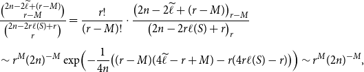
In particular, using Lemmas 2.2 and 2.3, if $r=O(\sqrt n)$
, then
$r=O(\sqrt n)$
, then
 \begin{align} \operatorname{\mathbb E}{}[(X_{S,n})_r] \sim (2n)^{2r-r}\exp \Bigl (-\frac{4r^2}{4n}+\frac{r^2}{4n}\Bigr )2^{-4r} = \left ( \frac{n}{8} \right )^r \exp \left ( -\frac{3r^2}{4n} \right ) . \end{align}
In other words, (2.2) holds (uniformly) for $0\le r\le C\sqrt n$
, for any fixed
$0\le r\le C\sqrt n$
, for any fixed $C\lt \infty$
, with
$C\lt \infty$
, with
 \begin{align} \mu _n&\;:\!=\;\frac{n}{8}, \end{align}
 \begin{align} s_n&\;:\!=\;-\frac{3}{2n}. \end{align}
We have $\mu _ns_n=-3/16\gt -1$
, and thus
$\mu _ns_n=-3/16\gt -1$
, and thus
 \begin{align} \sigma _n\;:\!=\;\sqrt{\mu _n(1+\mu _ns_n)}=\sqrt{\frac{13}{128} n}. \end{align}
We thus have $\sigma _n=o(\mu _n)$
and
$\sigma _n=o(\mu _n)$
and $\mu _n=o(\sigma _n^3)$
, and consequently Theorem 2.1 applies and yields:
$\mu _n=o(\sigma _n^3)$
, and consequently Theorem 2.1 applies and yields:
Theorem 3.1.
If $S$
is a simple loop of half-length 1, then
$S$
is a simple loop of half-length 1, then
 \begin{align} \frac{X_{S,n}-n/8}{\sqrt{13 n/128}} \underset{n \rightarrow \infty }{\overset{(d)}{\longrightarrow }} \mathcal{N}(0,1). \end{align}
This is Theorem 1.2 for this particular choice of $S$
, with
$S$
, with $\mu _S=1/8$
and
$\mu _S=1/8$
and $\sigma ^2_S=13/128$
.
$\sigma ^2_S=13/128$
.
4. Extension to any fixed shape
Let us now show how we can extend this result to any fixed shape $S$
. We now let
$S$
. We now let $Y_i$
be the indicator that there is a component
$Y_i$
be the indicator that there is a component $C$
of shape
$C$
of shape $S$
such that
$S$
such that $L_C=i$
; note that (3.1) and (3.2) still hold.
$L_C=i$
; note that (3.1) and (3.2) still hold.
Recall that $\ell (S)$
is the half-length of
$\ell (S)$
is the half-length of $S$
, so
$S$
, so $S$
has base
$S$
has base $[\![ 1,2\ell (S) ]\!]$
. We also define here three other constants
$[\![ 1,2\ell (S) ]\!]$
. We also define here three other constants $K(S), c_+(S), c_-(S)$
depending on
$K(S), c_+(S), c_-(S)$
depending on $S$
. To avoid heavy notation, we will drop the argument
$S$
. To avoid heavy notation, we will drop the argument $S$
in what follows and only denote them by
$S$
in what follows and only denote them by $K,c_+, c_-$
.
$K,c_+, c_-$
.
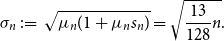
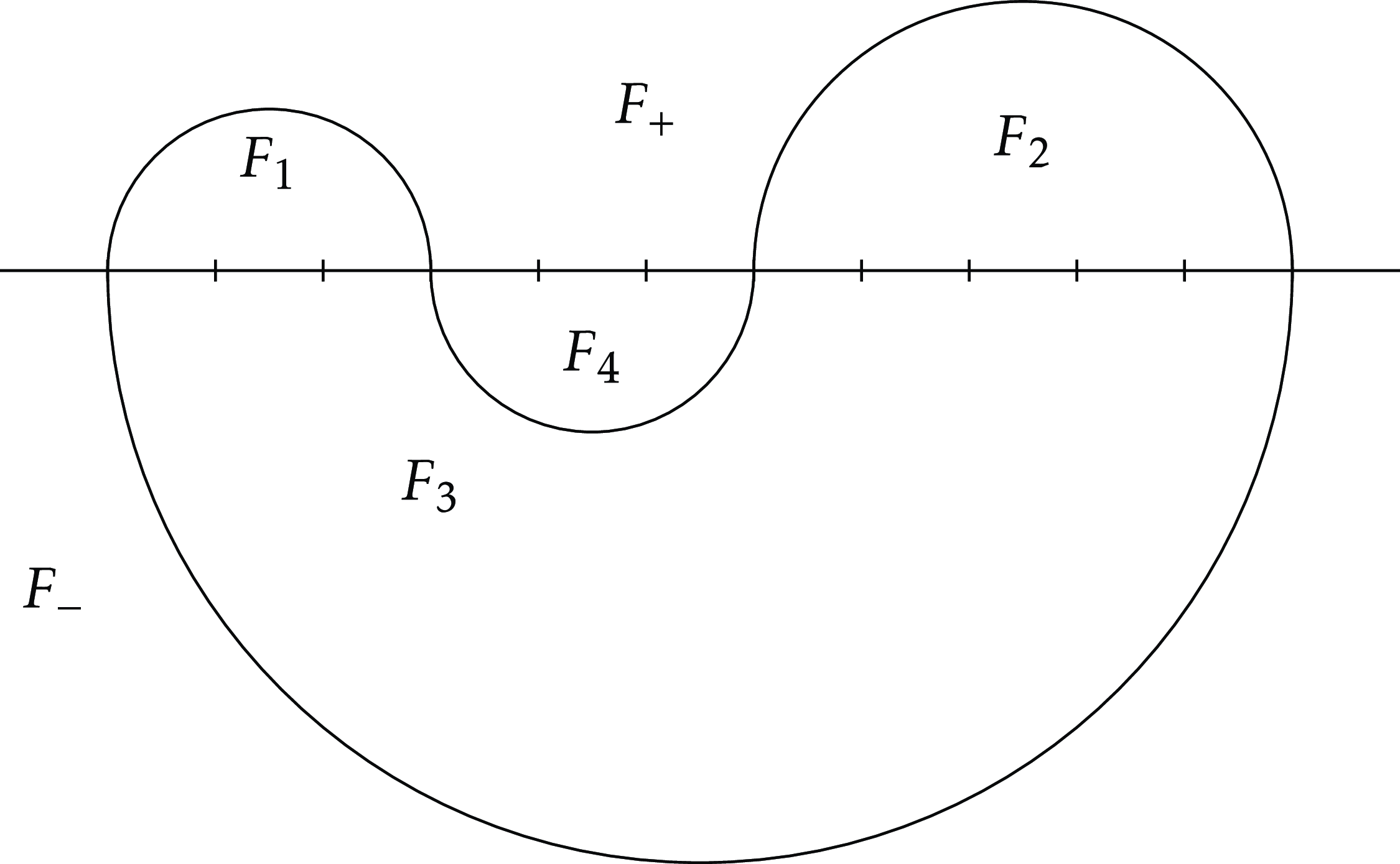
Definition 4.1.
(See an example in Figure
1
) Observe that a component $C$
of shape
$C$
of shape $S$
, taken along with the horizontal axis, splits the plane into two unbounded faces, each belonging to one of the half-planes, and a certain number of bounded faces. Let
$S$
, taken along with the horizontal axis, splits the plane into two unbounded faces, each belonging to one of the half-planes, and a certain number of bounded faces. Let $F_+$
denote the unbounded face in the upper half-plane,
$F_+$
denote the unbounded face in the upper half-plane, $F_-$
the one in the lower half-plane, and
$F_-$
the one in the lower half-plane, and $\mathcal{F}(C)$
the set of bounded faces. For a face
$\mathcal{F}(C)$
the set of bounded faces. For a face $F$
, let
$F$
, let $\nu (F)$
be the number of vertices in
$\nu (F)$
be the number of vertices in $[\![ L_C,R_C ]\!]$
that lie on the boundary of
$[\![ L_C,R_C ]\!]$
that lie on the boundary of $F$
but not on
$F$
but not on $C$
, and observe that necessarily
$C$
, and observe that necessarily $\nu (F)$
is even. We then set
$\nu (F)$
is even. We then set
 \begin{align} K(S) &\;:\!=\; \prod _{F \in \mathcal{F}(C)} \mathrm{Cat}_{\nu (F)/2}, \end{align}
 \begin{align} c_+(S)& \;:\!=\; \nu (F_+)/2, \end{align}
 \begin{align} c_-(S)& \;:\!=\; \nu (F_-)/2. \end{align}
Note that these constants do not depend on the set of vertices on which $C$
is defined, but only on its shape
$C$
is defined, but only on its shape $S$
.
$S$
.
4.1 Strong shapes
We say that two components overlap if their bases overlap. Hence, if the components have the same shape $S$
, and the leftmost points in their supports are
$S$
, and the leftmost points in their supports are $i$
and
$i$
and $j$
, they overlap if
$j$
, they overlap if $|j-i|\lt 2\ell (S)$
.
$|j-i|\lt 2\ell (S)$
.
A component $C$
with four bounded faces
$C$
with four bounded faces $F_1, F_2, F_3, F_4$
. In this example, we have
$F_1, F_2, F_3, F_4$
. In this example, we have $K(S)=\mathrm{Cat}_1^2 \mathrm{Cat}_2 \mathrm{Cat}_3=10$
,
$K(S)=\mathrm{Cat}_1^2 \mathrm{Cat}_2 \mathrm{Cat}_3=10$
, $c_+(S)=1$
, and
$c_+(S)=1$
, and $c_-(S)=0$
, where
$c_-(S)=0$
, where $S$
is the shape of
$S$
is the shape of $C$
.
$C$
.
For simplicity, we study first the case when this cannot happen. We say that a shape $S$
is strong if two different components of a meandric system that both have shape
$S$
is strong if two different components of a meandric system that both have shape $S$
cannot overlap. Thus, if
$S$
cannot overlap. Thus, if $S$
is strong, then
$S$
is strong, then $Y_iY_j=0$
when
$Y_iY_j=0$
when $|j-i|\lt 2\ell (S)$
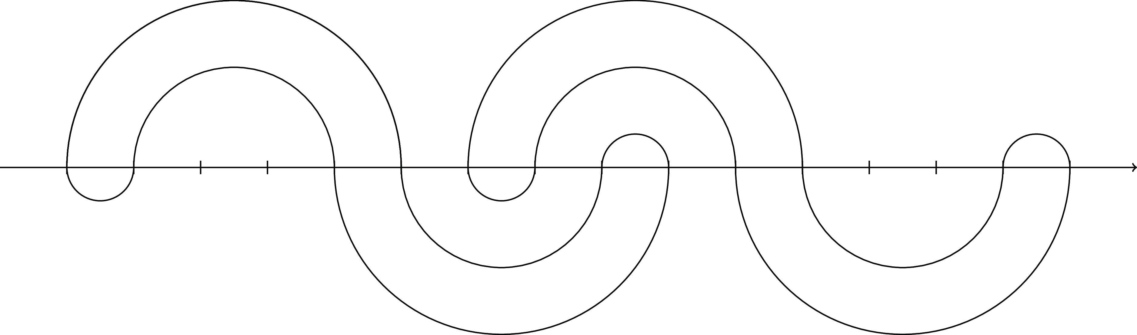
. The simple loop in Section 3 and the loop in Fig. 1 are examples of strong shapes. A shape that is not strong is called weak; an example is given in Fig. 2.
$|j-i|\lt 2\ell (S)$
. The simple loop in Section 3 and the loop in Fig. 1 are examples of strong shapes. A shape that is not strong is called weak; an example is given in Fig. 2.
Proposition 4.2.
Let $S$
be a strong shape of half-length
$S$
be a strong shape of half-length $\ell (S)$
. Then, for all
$\ell (S)$
. Then, for all $r \geq 1$
, we have
$r \geq 1$
, we have
 \begin{equation} \operatorname{\mathbb E}{}[(X_{S,n})_r] =\bigl (2n-2r\ell (S)+r\bigr )_{r} \, K^r \, \frac{\mathrm{Cat}_{n-r\ell (S) + r c_+} \mathrm{Cat}_{n- r \ell (S) + r c_-}}{\mathrm{Cat}_n^2}. \end{equation}
Proof. We argue as in Section 3. As noted above, (3.2) still holds, and since $S$
is strong, we have
$S$
is strong, we have $Y_iY_j=0$
when
$Y_iY_j=0$
when $|j-i|\lt 2\ell (S)$
. Hence, the number of non-zero terms in (3.2) is
$|j-i|\lt 2\ell (S)$
. Hence, the number of non-zero terms in (3.2) is $\binom{2n-r(2\ell (S)-1)}{r}$
by Lemma 2.4. Again, all non-zero terms have the same value, which is
$\binom{2n-r(2\ell (S)-1)}{r}$
by Lemma 2.4. Again, all non-zero terms have the same value, which is $1/\mathrm{Cat}_n^2$
times the number of ways that
$1/\mathrm{Cat}_n^2$
times the number of ways that $r$
given disjoint loops of shape
$r$
given disjoint loops of shape $S$
can be completed to a meandric system of size
$S$
can be completed to a meandric system of size $n$
. We can fill in the bounded faces of each component in
$n$
. We can fill in the bounded faces of each component in $K$
ways, and there are
$K$
ways, and there are $2n-2r\ell (S)+2rc_\pm$
vertices left in the upper and lower components, respectively, so they may be filled in
$2n-2r\ell (S)+2rc_\pm$
vertices left in the upper and lower components, respectively, so they may be filled in $\mathrm{Cat}_{n-r\ell (S)+rc_\pm }$
ways. This yields (4.4).
$\mathrm{Cat}_{n-r\ell (S)+rc_\pm }$
ways. This yields (4.4).
By Lemmas 2.2 and 2.3, it follows from (4.4) that, (uniformly) for $r=O(\sqrt{n})$
, we have
$r=O(\sqrt{n})$
, we have
 \begin{align} \operatorname{\mathbb E}{}[(X_{S,n})_r] \underset{n \rightarrow \infty }{\sim } \left ( \frac{2n K}{4^{2\ell (S)-c_+-c_-}} \right )^r \exp \left ( -\frac{r^2}{4n} \left [ (2\ell (S))^2 - (2\ell (S)-1)^2 \right ] \right ) . \end{align}
This is (2.2) with
 \begin{align} \mu _n&\;:\!=\;\frac{2n K}{4^{2\ell (S)-c_+-c_-}}, \end{align}
 \begin{align} s_n&\;:\!=\;-\frac{(2\ell (S))^2-(2\ell (S)-1)^2)}{2n} =-\frac{4\ell (S)-1}{2n}. \end{align}
In order to apply Theorem 2.1, we need to check that $\mu _ns_n \gt -1$
, which boils down to the following.
$\mu _ns_n \gt -1$
, which boils down to the following.
Two components of same shape overlapping. Here, $\operatorname{\mathbb E}{}[Y_1 Y_7]\gt 0$
, while
$\operatorname{\mathbb E}{}[Y_1 Y_7]\gt 0$
, while $2\ell (S)=10$
.
$2\ell (S)=10$
.
Lemma 4.3. We have
 \begin{equation} K (4\ell (S)-1) \lt 4^{2\ell (S)-c_+-c_-} . \end{equation}
Proof. Observe that we can bound $K$
using the fact that
$K$
using the fact that $\mathrm{Cat}_n \leq \frac{4^n}{n+1}$
for all
$\mathrm{Cat}_n \leq \frac{4^n}{n+1}$
for all $n$
. It is easy to see that for given
$n$
. It is easy to see that for given $c_\pm$
, out of all possible choices of components with these values of
$c_\pm$
, out of all possible choices of components with these values of $c_{\pm }$
,
$c_{\pm }$
, $K$
is largest if there is only one bounded face in each half-plane, and thus,
$K$
is largest if there is only one bounded face in each half-plane, and thus,
 \begin{align} K \leq \mathrm{Cat}_{\ell (S)-c_+-1} \mathrm{Cat}_{\ell (S)-c_- -1} \leq \frac{4^{2\ell (S)-c_+-c_- -2}}{(\ell (S)-c_+)(\ell (S)-c_-)} \leq \frac{4^{2\ell (S)-c_+-c_- -2}}{\ell (S)}, \end{align}
since $c_++c_- \leq \ell (S)-1$
(to see this, observe that a vertex cannot belong to both unbounded faces of
$c_++c_- \leq \ell (S)-1$
(to see this, observe that a vertex cannot belong to both unbounded faces of $S$
and that at least two vertices belong to
$S$
and that at least two vertices belong to $C$
). This yields (4.8) directly.
$C$
). This yields (4.8) directly.
It is clear that $\mu _n \rightarrow \infty$
. Furthermore, we have just proved that
$\mu _n \rightarrow \infty$
. Furthermore, we have just proved that $1+ \mu _n s_n$
is a positive constant. Thus
$1+ \mu _n s_n$
is a positive constant. Thus $\sigma _n=\Theta (\sqrt{\mu _n})$
, and hence
$\sigma _n=\Theta (\sqrt{\mu _n})$
, and hence $\sigma _n=o(\mu _n)$
and
$\sigma _n=o(\mu _n)$
and $\mu _n = o(\sigma _n^3)$
. We can therefore apply Theorem 2.1 to obtain the central limit theorem in this case too:
$\mu _n = o(\sigma _n^3)$
. We can therefore apply Theorem 2.1 to obtain the central limit theorem in this case too:
Theorem 4.4.
Let $S$
be a strong shape. Then
$S$
be a strong shape. Then
 \begin{align} \frac{X_{S,n} - n \mu _S}{\sigma _S\sqrt{n}} \underset{n \longrightarrow \infty }{\overset{(d)}{\rightarrow }} \mathcal{N}(0,1), \end{align}
where
 \begin{align} \mu _S = \frac{2K}{4^{2\ell (S)-c_+-c_-}} \quad \textrm{and}\quad \sigma _S = \sqrt{\frac{2K}{4^{2\ell (S)-c_+-c_-}} \Bigl (1- \frac{K(4\ell (S)-1)}{4^{2\ell (S)-c_+-c_-}} \Bigr )} . \end{align}
This proves Theorem 1.2 in the case when $S$
is a strong shape, with explicit formulas for
$S$
is a strong shape, with explicit formulas for $\mu _S$
and
$\mu _S$
and $\sigma _S$
.
$\sigma _S$
.
4.2 Weak shapes
Finally, we study the case of a weak shape $S$
. Thus, now there may be overlaps between two components of shape
$S$
. Thus, now there may be overlaps between two components of shape $S$
, that is, two indices
$S$
, that is, two indices $i\lt j$
such that
$i\lt j$
such that $|j-i|\lt 2\ell (S)$
and
$|j-i|\lt 2\ell (S)$
and $Y_i Y_j=1$
, where
$Y_i Y_j=1$
, where $Y_i$
is defined as before. See Fig. 2 for an example.
$Y_i$
is defined as before. See Fig. 2 for an example.
Let $A^r$
be the set of all
$A^r$
be the set of all $r$
-tuples
$r$
-tuples $ E \;:\!=\; \{ i_1, \ldots, i_r \}$
with
$ E \;:\!=\; \{ i_1, \ldots, i_r \}$
with $1 \leq i_1\lt \cdots \lt i_r \leq 2n$
. For any such
$1 \leq i_1\lt \cdots \lt i_r \leq 2n$
. For any such $r$
-tuple
$r$
-tuple $E$
, define an equivalence relation
$E$
, define an equivalence relation $\sim _E$
on
$\sim _E$
on $\{ 1,\ldots, r \}$
as the smallest one (for the inclusion of the equivalence classes) satisfying: for all
$\{ 1,\ldots, r \}$
as the smallest one (for the inclusion of the equivalence classes) satisfying: for all $1 \leq k_1, k_2 \leq r$
such that
$1 \leq k_1, k_2 \leq r$
such that $|i_{k_1} - i_{k_2}| \lt 2\ell (S)$
,
$|i_{k_1} - i_{k_2}| \lt 2\ell (S)$
, $k_1 \sim _E k_2$
. We call the equivalence classes of
$k_1 \sim _E k_2$
. We call the equivalence classes of $\sim _E$
blocks. Furthermore, for
$\sim _E$
blocks. Furthermore, for $1 \leq j \leq r$
, we let
$1 \leq j \leq r$
, we let $A^r_j$
be the set of
$A^r_j$
be the set of $r$
-tuples
$r$
-tuples $E\in A^r$
that have exactly
$E\in A^r$
that have exactly $j$
blocks. Thus
$j$
blocks. Thus $A^r=\bigsqcup _{j=1}^r A^r_j$
. Note that
$A^r=\bigsqcup _{j=1}^r A^r_j$
. Note that $A^r_r$
is the set of
$A^r_r$
is the set of $r$
-tuples
$r$
-tuples $E$
such that all blocks are singletons. An
$E$
such that all blocks are singletons. An $r$
-tuple
$r$
-tuple $E$
corresponds to a collection
$E$
corresponds to a collection $(C_k)_1^r$
of loops of shape
$(C_k)_1^r$
of loops of shape $S$
, shifted such that
$S$
, shifted such that $C_k$
has
$C_k$
has $L_{C_k}=i_k$
. In particular,
$L_{C_k}=i_k$
. In particular, $E\in A_r^r$
if and only if these loops are non-overlapping.
$E\in A_r^r$
if and only if these loops are non-overlapping.
Define, for all $1 \leq u \leq r$
:
$1 \leq u \leq r$
:
 \begin{align} F_u \;:\!=\; \binom{2n-2u\ell (S)+u}{u} \, K^u \, \frac{\mathrm{Cat}_{n-u\ell (S) + u c_+} \mathrm{Cat}_{n- u \ell (S) + u c_-}}{\mathrm{Cat}_n^2}. \end{align}
By the argument in the proof of Proposition 4.2, $u!\,F_u$
is the contribution to
$u!\,F_u$
is the contribution to $\operatorname{\mathbb E}{}[(X_{S,n})_u]$
from
$\operatorname{\mathbb E}{}[(X_{S,n})_u]$
from $u$
-tuples of non-overlapping components.
$u$
-tuples of non-overlapping components.
We have the following estimates:
Lemma 4.5.
Let $S$
be a weak shape.
$S$
be a weak shape.
-
(i) For all
$r\ge 1$
,(4.13)
\begin{equation} \operatorname{\mathbb E}{}[(X_{S,n})_r] \geq r! F_r. \end{equation}
-
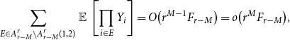
(ii) For all
$1 \leq u \leq r$
,(4.14)
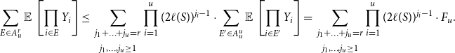
\begin{align} \sum _{E \in A^r_u} \operatorname{\mathbb E}{}\left [\prod _{i \in E}Y_i\right ] &\leq \binom{r-1}{u-1} (2\ell (S))^{r-u} F_u. \end{align}
-
(iii) For each fixed
$M \geq 0$
, uniformly for
$r=O(\sqrt{n})$
with
$r\ge 2M$
,(4.15)and, if also
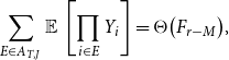
\begin{align} \sum _{E \in A^r_{r-M}} \operatorname{\mathbb E}{}\left [\prod _{i \in E}Y_i\right ] = \Theta \left (r^M F_{r-M}\right ) \end{align}
$r\to \infty$
,(4.16)where
\begin{align} \sum _{E \in A^r_{r-M}(1,2)} \operatorname{\mathbb E}{}\left [ \prod _{i \in E} Y_i \right ] = (1-o(1))\sum _{E \in A^r_{r-M}} \operatorname{\mathbb E}{}\left [ \prod _{i \in E} Y_i \right ], \end{align}
$A^r_{r-M}(1,2)$
is the subset of
$A^r_{r-M}$
made only of blocks of sizes
$1$
or
$2$
.


Proof of Lemma 4.5. (i): We rewrite (3.2) as
 \begin{align} \operatorname{\mathbb E}{}\left [ (X_{S,n})_r \right ] =r! \sum _{E \in A^r} \operatorname{\mathbb E}{}\left [ \prod _{i \in E} Y_i \right ] = r!\sum _{u=1}^r\sum _{E \in A^r_u} \operatorname{\mathbb E}{}\left [ \prod _{i \in E} Y_i \right ]. \end{align}
The term with $u=r$
yields the contribution from
$u=r$
yields the contribution from $r$
-tuples of non-overlapping components, which as noted after (4.12) is
$r$
-tuples of non-overlapping components, which as noted after (4.12) is $r! F_r$
.
$r! F_r$
.
(ii): For each $r$
-tuple
$r$
-tuple $E\in A^r_u$
, keep in the product only the leftmost point of each block, observing that, for any sets
$E\in A^r_u$
, keep in the product only the leftmost point of each block, observing that, for any sets $A \subseteq B \subseteq [\![ 1, 2n ]\!]$
, we have
$A \subseteq B \subseteq [\![ 1, 2n ]\!]$
, we have $\operatorname{\mathbb E}{}\left [ \prod _{i \in B} Y_i \right ] \leq \operatorname{\mathbb E}{}\left [ \prod _{i \in A} Y_i\right ]$
. Note that this set of leftmost points belongs to
$\operatorname{\mathbb E}{}\left [ \prod _{i \in B} Y_i \right ] \leq \operatorname{\mathbb E}{}\left [ \prod _{i \in A} Y_i\right ]$
. Note that this set of leftmost points belongs to $A^u_u$
. If the size of the
$A^u_u$
. If the size of the $i$
-th leftmost block is
$i$
-th leftmost block is $j_i$
, then for each set of leftmost points, the number of possible positions of the other
$j_i$
, then for each set of leftmost points, the number of possible positions of the other $j_i-1$
points in the block is at most
$j_i-1$
points in the block is at most $(2\ell (S))^{j_i-1}$
, since each point after the first is within
$(2\ell (S))^{j_i-1}$
, since each point after the first is within $2\ell (S)$
of the preceding one. Hence,
$2\ell (S)$
of the preceding one. Hence,
 \begin{align} \sum _{E \in A^r_u} \operatorname{\mathbb E}{}\left [\prod _{i \in E}Y_i\right ] &\leq \, \sum _{\substack{j_1+\ldots +j_u=r \\[5pt] j_1, \ldots, j_u \geq 1}}{\prod _{i=1}^u (2\ell (S))^{j_i-1} }\cdot \sum _{E' \in A^u_u} \operatorname{\mathbb E}{}\left [\prod _{i \in E'}Y_i\right ] = \, \sum _{\substack{j_1+\ldots +j_u=r \\[5pt] j_1, \ldots, j_u \geq 1}}{\prod _{i=1}^u (2\ell (S))^{j_i-1} }\cdot F_u . \end{align}
Finally, this yields (4.14), since the number of allowed sequences $(j_1,\dots,j_u)$
is
$(j_1,\dots,j_u)$
is $\binom{r-1}{u-1}$
and
$\binom{r-1}{u-1}$
and $\prod _{i=1}^u (2\ell (S))^{j_i-1} =(2\ell (S))^{r-u}$
for all of them.
$\prod _{i=1}^u (2\ell (S))^{j_i-1} =(2\ell (S))^{r-u}$
for all of them.
(iii): We partition the set $A^r_{r-M}$
as follows. Consider an
$A^r_{r-M}$
as follows. Consider an $(r-M)$
-tuple
$(r-M)$
-tuple $T \;:\!=\; (T_1, \ldots, T_{r-M})$
of integers
$T \;:\!=\; (T_1, \ldots, T_{r-M})$
of integers $\geq 1$
, of sum
$\geq 1$
, of sum $r$
, and consider also a function
$r$
, and consider also a function $J$
which, to each
$J$
which, to each $1 \leq i \leq r-M$
, associates a
$1 \leq i \leq r-M$
, associates a $T_i$
-tuple
$T_i$
-tuple $J_i$
of integers
$J_i$
of integers $1 \;=\!:\;\, j_{i,1} \lt j_{i,2} \lt \ldots \lt j_{i,T_i}$
such that, for all
$1 \;=\!:\;\, j_{i,1} \lt j_{i,2} \lt \ldots \lt j_{i,T_i}$
such that, for all $1 \leq k \leq T_i-1$
,
$1 \leq k \leq T_i-1$
, $j_{i,k+1}-j_{i,k} \lt 2\ell (S)$
, and, furthermore, the
$j_{i,k+1}-j_{i,k} \lt 2\ell (S)$
, and, furthermore, the $T_i$
loops of shape
$T_i$
loops of shape $S$
that start at the vertices
$S$
that start at the vertices $j_{i,k}$
(
$j_{i,k}$
( $k=1,\dots,T_i$
) are disjoint so that they may occur together as components in a meandric system. (We call such pairs
$k=1,\dots,T_i$
) are disjoint so that they may occur together as components in a meandric system. (We call such pairs $(T,J)$
admissible.) Denote by
$(T,J)$
admissible.) Denote by $A_{T,J}$
the subset of
$A_{T,J}$
the subset of $A^r_{r-M}$
made of
$A^r_{r-M}$
made of $r$
-tuples
$r$
-tuples $E$
such that the
$E$
such that the $i$
-th leftmost block of
$i$
-th leftmost block of $E$
has size
$E$
has size $T_i$
, and if this block is
$T_i$
, and if this block is $\left \{a^1_i, \ldots, a^{T_i}_i\right \}$
, then we have
$\left \{a^1_i, \ldots, a^{T_i}_i\right \}$
, then we have $a_i^{k+1}-a_i^k = j_{i,k+1}-j_{i,k}$
for all
$a_i^{k+1}-a_i^k = j_{i,k+1}-j_{i,k}$
for all $1 \leq k \leq T_i-1$
. In other words,
$1 \leq k \leq T_i-1$
. In other words, $A_{T,J}$
accounts for all
$A_{T,J}$
accounts for all $r$
-tuples of components with
$r$
-tuples of components with $r-M$
blocks, where the sizes of the blocks are given, as well as the intervals between the starting points of each component of shape
$r-M$
blocks, where the sizes of the blocks are given, as well as the intervals between the starting points of each component of shape $S$
in each block. Hence,
$S$
in each block. Hence, $A^r_{r-M}$
is the union
$A^r_{r-M}$
is the union $\bigcup A_{T,J}$
over all admissible pairs
$\bigcup A_{T,J}$
over all admissible pairs $(T,J)$
.
$(T,J)$
.
Since we only consider $(r-M)$
-tuples
$(r-M)$
-tuples $T$
such that
$T$
such that
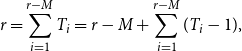 \begin{align} r=\sum _{i=1}^{r-M} T_i = r-M+\sum _{i=1}^{r-M} (T_i-1), \end{align}
there at most $M$
indices
$M$
indices $i$
with
$i$
with $T_i\gt 1$
and thus at least
$T_i\gt 1$
and thus at least $r-2M$
indices with
$r-2M$
indices with $T_i=1$
. Note also that if
$T_i=1$
. Note also that if $T_i=1$
, then trivially,
$T_i=1$
, then trivially, $J_i=(1)$
. Given an admissible pair
$J_i=(1)$
. Given an admissible pair $(T,J)$
, we define the reduced pair
$(T,J)$
, we define the reduced pair $(\widehat{T},\widehat{J})$
by deleting all
$(\widehat{T},\widehat{J})$
by deleting all $T_i$
and
$T_i$
and $J_i$
such that
$J_i$
such that $T_i=1$
from
$T_i=1$
from $T$
and
$T$
and $J$
; thus
$J$
; thus $\widehat{T}\;:\!=\;(T_i\;:\;1\le i\le r-M \textrm{ and }T_i\gt 1)$
and similarly for
$\widehat{T}\;:\!=\;(T_i\;:\;1\le i\le r-M \textrm{ and }T_i\gt 1)$
and similarly for $\widehat{J}$
. Consequently,
$\widehat{J}$
. Consequently, $\widehat{T}$
and
$\widehat{T}$
and $\widehat{J}$
are both sequences of (the same) length
$\widehat{J}$
are both sequences of (the same) length $\le M$
. Since (4.19) implies that their entries are bounded (for a fixed
$\le M$
. Since (4.19) implies that their entries are bounded (for a fixed $M$
), there is only a finite set
$M$
), there is only a finite set $\mathcal{T}$
of reduced pairs
$\mathcal{T}$
of reduced pairs $(\widehat{T},\widehat{J})$
, where
$(\widehat{T},\widehat{J})$
, where $\mathcal{T}$
depends on
$\mathcal{T}$
depends on $M$
and
$M$
and $S$
but not on
$S$
but not on $r$
.
$r$
.
Conversely, given an admissible reduced pair $(\widehat{T},\widehat{J})$
, with
$(\widehat{T},\widehat{J})$
, with $\widehat{T}=(\widehat{T}_1,\dots,\widehat{T}_k)$
, we can obtain
$\widehat{T}=(\widehat{T}_1,\dots,\widehat{T}_k)$
, we can obtain $(\widehat{T},\widehat{J})$
from
$(\widehat{T},\widehat{J})$
from $\binom{r-M}{k}$
different (admissible) pairs
$\binom{r-M}{k}$
different (admissible) pairs $(T,J)$
. Note that here, by (4.19), since each
$(T,J)$
. Note that here, by (4.19), since each $\widehat{T}_i\ge 2$
,
$\widehat{T}_i\ge 2$
,
 \begin{align} k \le \sum _{i=1}^k(\widehat{T}_i-1) = \sum _{i=1}^{r-M}(T_i-1)=M, \end{align}
with equality if and only if $\widehat{T}_i=2$
for all
$\widehat{T}_i=2$
for all $i\le k$
.
$i\le k$
.
We now want to understand the behaviour of $\sum _{E \in A_{T,J}} \operatorname{\mathbb E}{} \left [ \prod _{i \in E} Y_i \right ]$
for an admissible pair
$\sum _{E \in A_{T,J}} \operatorname{\mathbb E}{} \left [ \prod _{i \in E} Y_i \right ]$
for an admissible pair $(T,J)$
. In a way similar to Proposition 4.2 (using an extension of Lemma 2.4 to intervals of different lengths), we obtain
$(T,J)$
. In a way similar to Proposition 4.2 (using an extension of Lemma 2.4 to intervals of different lengths), we obtain
 \begin{align} \sum _{E \in A_{T,J}} \operatorname{\mathbb E}{} \left [ \prod _{i \in E} Y_i \right ] = \binom{2n-2\widetilde{\ell }+(r-M)}{r-M}\, \widetilde{K}\, \frac{\mathrm{Cat}_{n-d_+} \mathrm{Cat}_{n-d_-}}{\mathrm{Cat}_n^2}, \end{align}
where, for any $E\in A_{T,J}$
,
$E\in A_{T,J}$
, $\widetilde{\ell }$
is the sum of the half-lengths of the blocks,
$\widetilde{\ell }$
is the sum of the half-lengths of the blocks, $\widetilde{K}$
accounts for the bounded faces defined by the horizontal axis and the loops defined by
$\widetilde{K}$
accounts for the bounded faces defined by the horizontal axis and the loops defined by $E$
, and
$E$
, and $d_+, d_-$
for the unbounded faces. (Note that these constants are the same for all
$d_+, d_-$
for the unbounded faces. (Note that these constants are the same for all $E\in A_{T,J}$
, so they depend only on
$E\in A_{T,J}$
, so they depend only on $T$
and
$T$
and $J$
.) Moreover, since at least
$J$
.) Moreover, since at least $r-2M$
of these blocks are singletons, and the remaining blocks are determined by
$r-2M$
of these blocks are singletons, and the remaining blocks are determined by $\widehat{T}$
and
$\widehat{T}$
and $\widehat{J}$
, we can write
$\widehat{J}$
, we can write
 \begin{align} \widetilde{K} = K^{r-2M} K', \end{align}
for some $K'\gt 0$
depending only on
$K'\gt 0$
depending only on $(\widehat{T},\widehat{J})$
. Similarly,
$(\widehat{T},\widehat{J})$
. Similarly,
 \begin{align} \widetilde{\ell } &= (r-M) \ell (S) + \ell ', \end{align}
 \begin{align} d_+&=(r-M)(\ell (S) - c_+) + e_+, \end{align}
 \begin{align} d_-& = (r-M)(\ell (S)-c_-)+e_- \end{align}
for some $\ell ', e_+,e_-$
depending only on
$\ell ', e_+,e_-$
depending only on $(\widehat{T},\widehat{J})$
. In particular, for a fixed
$(\widehat{T},\widehat{J})$
. In particular, for a fixed $M$
, it follows that
$M$
, it follows that $K', \ell ', e_+, e_-$
can only take a fixed number of values independently of
$K', \ell ', e_+, e_-$
can only take a fixed number of values independently of $n$
and
$n$
and $r$
.
$r$
.
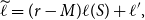
We compare (4.21) and $F_{r-M}$
given by (4.12). First, by Lemma 2.2(iii),
$F_{r-M}$
given by (4.12). First, by Lemma 2.2(iii),
 \begin{align} & \frac{\binom{2n-2\widetilde{\ell } + (r-M)}{r-M}}{\binom{2n-2(r-M) \ell (S) + (r-M)}{r-M}} = \frac{\bigl (2n-2\widetilde{\ell } + (r-M)\bigr )_{r-M}}{\bigl (2n-2(r-M) \ell (S) + (r-M)\bigr )_{r-M}} \\[5pt] \notag &\hskip 4em \sim \exp \Bigl (-\frac{r-M}{4n} \bigl ((4\widetilde{\ell }-r+M)-(4(r-M)\ell (S)-r+M)\bigr )\Bigr ) =\exp \bigl (o(1)\bigr ), \end{align}
since $\widetilde{\ell }=r\ell (S)+O(1)$
by (4.23) and
$\widetilde{\ell }=r\ell (S)+O(1)$
by (4.23) and $r=o(n)$
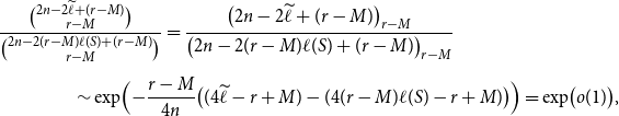
. Similarly, as a consequence of Lemma 2.3 and (4.24)–(4.25),
$r=o(n)$
. Similarly, as a consequence of Lemma 2.3 and (4.24)–(4.25),
 \begin{align} &\frac{\mathrm{Cat}_{n-d_\pm }}{\mathrm{Cat}_{n-(r-M)(\ell (S)-c_\pm )}} \sim 4^{-d_\pm +(r-M)(\ell (S)-c_\pm )}=4^{-e_\pm }. \end{align}
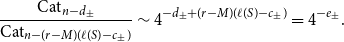
Consequently, using also (4.22), we obtain from (4.21) and (4.12),
 \begin{align} \frac{\sum _{E \in A_{T,J}} \operatorname{\mathbb E}{} \left [ \prod _{i \in E} Y_i \right ]}{F_{r-M}} = C_{T,J} (1+o(1)), \end{align}
where $C_{T,J}\gt 0$
only depends on
$C_{T,J}\gt 0$
only depends on $(\widehat{T},\widehat{J})$
and therefore only takes a finite number of values. In particular,
$(\widehat{T},\widehat{J})$
and therefore only takes a finite number of values. In particular,
 \begin{align} \sum _{E \in A_{T,J}} \operatorname{\mathbb E}{} \left [ \prod _{i \in E} Y_i \right ]=\Theta \bigl (F_{r-M}\bigr ), \end{align}
and this holds uniformly for $r=O(\sqrt n)$
and all admissible
$r=O(\sqrt n)$
and all admissible $(T,J)$
.
$(T,J)$
.
By (4.20) and the discussion before it, there are $\binom{r-M}{k}=\Theta (r^k)$
admissible pairs
$\binom{r-M}{k}=\Theta (r^k)$
admissible pairs $(T,J)$
for each
$(T,J)$
for each $(\widehat{T},\widehat{J})$
, where
$(\widehat{T},\widehat{J})$
, where $k\le M$
, with equality when all
$k\le M$
, with equality when all $\widehat{T}_i=2$
. Note that since we assume that the shape
$\widehat{T}_i=2$
. Note that since we assume that the shape $S$
is weak, there exists at least one such admissible
$S$
is weak, there exists at least one such admissible $(\widehat{T},\widehat{J})$
with
$(\widehat{T},\widehat{J})$
with $\widehat{T}=(2,\dots,2)$
. Hence, summing (4.29) over all
$\widehat{T}=(2,\dots,2)$
. Hence, summing (4.29) over all $(T,J)$
yields (4.15).
$(T,J)$
yields (4.15).
Moreover, $A^r_{r-M}\setminus A^r_{r-M}(1,2)$
is the union
$A^r_{r-M}\setminus A^r_{r-M}(1,2)$
is the union $\bigcup ' A_{T,J}$
where we only sum over admissible pairs
$\bigcup ' A_{T,J}$
where we only sum over admissible pairs $(T,J)$
with some
$(T,J)$
with some $T_i\ge 3$
; these correspond to reduced pairs
$T_i\ge 3$
; these correspond to reduced pairs $(\widehat{T},\widehat{J})$
with some
$(\widehat{T},\widehat{J})$
with some $\widehat{T}_i\ge 3$
, and we see from (4.20) that each such reduced pair has length
$\widehat{T}_i\ge 3$
, and we see from (4.20) that each such reduced pair has length $\le M-1$
and thus corresponds to
$\le M-1$
and thus corresponds to $O(r^{M-1})$
admissible pairs. Consequently, summing (4.29) over all
$O(r^{M-1})$
admissible pairs. Consequently, summing (4.29) over all $(T,J)$
of this type yields
$(T,J)$
of this type yields
 \begin{align} \sum _{E \in A^r_{r-M}\setminus A^r_{r-M}(1,2)} \operatorname{\mathbb E}{}\left [ \prod _{i \in E} Y_i \right ] = O\bigl (r^{M-1}F_{r-M}\bigr ) = o\bigl (r^{M}F_{r-M}\bigr ), \end{align}
The next proposition shows that, in order to get the asymptotic behaviour of $\operatorname{\mathbb E}{}[(X_{S,n})_r]$
, we only need to take into account the configurations whose number of blocks that are not singletons is a given constant.
$\operatorname{\mathbb E}{}[(X_{S,n})_r]$
, we only need to take into account the configurations whose number of blocks that are not singletons is a given constant.
Proposition 4.6.
Fix a weak shape $S$
. Then, there exists
$S$
. Then, there exists $\eta \gt 0$
such that, for any
$\eta \gt 0$
such that, for any $\varepsilon \gt 0$
, there exists
$\varepsilon \gt 0$
, there exists $M\gt 0$
such that we have, uniformly for
$M\gt 0$
such that we have, uniformly for $r\le \eta \sqrt{n}$
,
$r\le \eta \sqrt{n}$
,
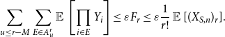 \begin{align} \sum _{u \leq r-M} \sum _{E \in A^r_u} \operatorname{\mathbb E}{}\left [\prod _{i \in E} Y_{i} \right ] \le \varepsilon F_r \leq \varepsilon \frac{1}{r!} \operatorname{\mathbb E}{}[(X_{S,n})_r]. \end{align}
Remark 4.7.
For convenience, we assume here that $r/\sqrt n$
is small. In fact, Proposition
4.6
can easily be extended to
$r/\sqrt n$
is small. In fact, Proposition
4.6
can easily be extended to $r\le C\sqrt n$
for any
$r\le C\sqrt n$
for any $C$
(with
$C$
(with $M$
depending on
$M$
depending on $C$
and
$C$
and $\varepsilon$
), but we do not need for this.
$\varepsilon$
), but we do not need for this.
To prove this, we start with a lemma:
Lemma 4.8.
There exists $Q \gt 0$
depending only on the shape
$Q \gt 0$
depending only on the shape $S$
such that, for
$S$
such that, for $n$
large enough, for all
$n$
large enough, for all $u \leq \sqrt{n}$
:
$u \leq \sqrt{n}$
:
 \begin{align} \frac{F_{u+1}}{F_u} \geq Q \frac{n}{u}. \end{align}
Proof. We just compute the ratio term by term, recalling (4.12). We have $\frac{K^{u+1}}{K^u} = K$
. The ratio of the ratios of Catalan numbers converges uniformly to a positive constant. Finally, the ratio of binomial coefficients is, using Lemma 2.2
(ii),
$\frac{K^{u+1}}{K^u} = K$
. The ratio of the ratios of Catalan numbers converges uniformly to a positive constant. Finally, the ratio of binomial coefficients is, using Lemma 2.2
(ii),
 \begin{align} \frac{u!}{(u+1)!}\cdot \frac{\bigl (2n-(u+1)(2\ell (S)-1)\bigr )_{u+1}}{\bigl (2n-u(2\ell (S)-1)\bigr )_u} =\frac{1}{u+1}\cdot \frac{(2n)^{u+1}}{(2n)^u}\exp \bigl (O(1)\bigr ) \ge c\frac{n}{u} \end{align}
for some $c\gt 0$
and all large
$c\gt 0$
and all large $n$
and
$n$
and $u\le \sqrt n$
. The result follows.
$u\le \sqrt n$
. The result follows.
Proof of Proposition
4.6. Using Lemma 4.5(ii), we have for all $M\geq 0$
:
$M\geq 0$
:
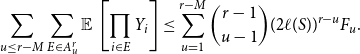 \begin{align} \sum _{u \leq r-M} \sum _{E \in A^r_u} \operatorname{\mathbb E}{}\left [\prod _{i \in E} Y_{i} \right ] &\le \sum _{u=1}^{r-M} \binom{r-1}{u-1} (2\ell (S))^{r-u} F_u. \end{align}
Letting
 \begin{align} B_{r,u} \;:\!=\; \binom{r-1}{u-1} (2\ell (S))^{r-u} F_u, \end{align}
we get from Lemma 4.8 that, for $r\le \sqrt n$
and any
$r\le \sqrt n$
and any $u \leq r-1$
:
$u \leq r-1$
:
 \begin{align} \frac{B_{r,u+1}}{B_{r,u}} = \frac{1}{2\ell (S)} \frac{r-u}{u} \frac{F_{u+1}}{F_u} \geq \frac{Q}{2\ell (S)} \frac{n(r-u)}{u^2} \geq \frac{Q}{2\ell (S)} \frac{n}{u^2} . \end{align}
Hence, there exists $\eta \gt 0$
small enough such that, for all
$\eta \gt 0$
small enough such that, for all $u \lt r \leq \eta \sqrt{n}$
, we have
$u \lt r \leq \eta \sqrt{n}$
, we have $B_{r,u+1} \geq 2 B_{r,u}$
, and thus by backward induction,
$B_{r,u+1} \geq 2 B_{r,u}$
, and thus by backward induction,
 \begin{align} B_{r,u} \le 2^{-(r-u)}B_{r,r} . \end{align}
Then, for $r\le \eta \sqrt n$
, (4.34) yields
$r\le \eta \sqrt n$
, (4.34) yields
 \begin{align} \sum _{u \leq r-M} \sum _{E \in A^r_u} \operatorname{\mathbb E}{}\left [\prod _{i \in E} Y_{i} \right ] &\le \sum _{u=1}^{r-M} B_{r,u} \le 2^{1-M} B_{r,r} =2^{1-M}F_r. \end{align}
This yields (4.31) if we choose $M$
such that
$M$
such that $2^{1-M}\le \varepsilon$
, since
$2^{1-M}\le \varepsilon$
, since $r!\,F_r \le \operatorname{\mathbb E}{}[(X_{S,n})_r]$
by Lemma 4.5(i).
$r!\,F_r \le \operatorname{\mathbb E}{}[(X_{S,n})_r]$
by Lemma 4.5(i).
Proposition 4.6 shows that we only need to understand the asymptotic behaviour of the configurations with a number of blocks $r-M$
for given
$r-M$
for given $M \geq 0$
, and Lemma 4.5(iii) that we can focus on configurations with blocks of size
$M \geq 0$
, and Lemma 4.5(iii) that we can focus on configurations with blocks of size $1$
or
$1$
or $2$
. To actually prove our final result, we need to refine Lemma 4.5(iii) and obtain the explicit constants that appear. We define another set of constants, which will account for the cases with blocks of size 2, that is, cases when two components of shape
$2$
. To actually prove our final result, we need to refine Lemma 4.5(iii) and obtain the explicit constants that appear. We define another set of constants, which will account for the cases with blocks of size 2, that is, cases when two components of shape $S$
overlap.
$S$
overlap.
Definition 4.9.
Let $S$
be a shape. There is a finite set of integers
$S$
be a shape. There is a finite set of integers $i \geq 1$
such that
$i \geq 1$
such that $\operatorname{\mathbb E}{}[Y_1 Y_i] \gt 0$
and
$\operatorname{\mathbb E}{}[Y_1 Y_i] \gt 0$
and $i-1 \lt 2\ell (S)$
. Let
$i-1 \lt 2\ell (S)$
. Let $I(S)$
be this set and
$I(S)$
be this set and $i_1, \ldots, i_k$
its elements. For
$i_1, \ldots, i_k$
its elements. For $i \in I(S)$
, let
$i \in I(S)$
, let $\ell _i$
,
$\ell _i$
, $K_i$
,
$K_i$
, $c_+(i)$
, and
$c_+(i)$
, and $c_-(i)$
be the equivalents of
$c_-(i)$
be the equivalents of $\ell (S), K, c_+, c_-$
in this case of two components
$\ell (S), K, c_+, c_-$
in this case of two components $C, C'$
that overlap and start at positions
$C, C'$
that overlap and start at positions $1$
and
$1$
and $i$
(replacing in the definition the component by the union of the two components). In particular,
$i$
(replacing in the definition the component by the union of the two components). In particular, $\ell _i = \ell (S) + (i-1)/2$
is the total half-length of the block made of two components of shape
$\ell _i = \ell (S) + (i-1)/2$
is the total half-length of the block made of two components of shape $S$
started at positions
$S$
started at positions $1$
and
$1$
and $i$
. Furthermore,
$i$
. Furthermore, $C$
and
$C$
and $C'$
together with the horizontal axis define two unbounded faces (
$C'$
together with the horizontal axis define two unbounded faces ( $F_+$
in the upper half-plane and
$F_+$
in the upper half-plane and $F_-$
in the lower half-plane) and several bounded faces; let
$F_-$
in the lower half-plane) and several bounded faces; let $\mathcal{F}(C,C')$
be the set of bounded faces. For each face
$\mathcal{F}(C,C')$
be the set of bounded faces. For each face $F$
, let
$F$
, let $\nu (F)$
be the number of integers in
$\nu (F)$
be the number of integers in $[\![ L(C),R(C) ]\!]\cup [\![ L(C'),R(C') ]\!] =[\![ L(C),R(C') ]\!]$
that are incident to
$[\![ L(C),R(C) ]\!]\cup [\![ L(C'),R(C') ]\!] =[\![ L(C),R(C') ]\!]$
that are incident to $F$
but do not belong to
$F$
but do not belong to $C$
nor to
$C$
nor to $C'$
. We set
$C'$
. We set $K_i \;:\!=\; \prod _{F \in \mathcal{F}(C, C')} \mathrm{Cat}_{\nu (F)/2}$
. Finally, we define
$K_i \;:\!=\; \prod _{F \in \mathcal{F}(C, C')} \mathrm{Cat}_{\nu (F)/2}$
. Finally, we define $c_\pm (i)\;:\!=\;\nu (F_\pm )/2$
. Observe again that all these constants only depend on
$c_\pm (i)\;:\!=\;\nu (F_\pm )/2$
. Observe again that all these constants only depend on $S$
and
$S$
and $i$
.
$i$
.
Note that $i\in I(S)$
may be even; in this case
$i\in I(S)$
may be even; in this case $2\ell _i$
,
$2\ell _i$
, $\nu (F_+)$
and
$\nu (F_+)$
and $\nu (F_-)$
are odd, and thus
$\nu (F_-)$
are odd, and thus $\ell _i$
and
$\ell _i$
and $c_\pm (i)$
are half-integers.
$c_\pm (i)$
are half-integers.
Lemma 4.10.
Let $r=O(\sqrt n)$
with
$r=O(\sqrt n)$
with $r\to \infty$
. Then, for every fixed
$r\to \infty$
. Then, for every fixed $M\ge 0$
,
$M\ge 0$
,
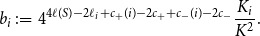
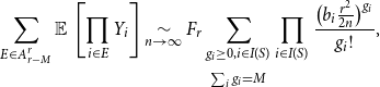 \begin{align} \sum _{E \in A^r_{r-M}} \operatorname{\mathbb E}{}\left [ \prod _{i \in E} Y_i \right ] \underset{n \rightarrow \infty }{\sim } F_r \sum _{\substack{g_i\ge 0, i\in I(S)\\[5pt] \sum _i g_i=M}} \prod _{i \in I(S)} \frac{\bigl (b_i\frac{r^2}{2n}\bigr )^{g_i}}{g_i!}, \end{align}
where
 \begin{align} b_i&\;:\!=\;4^{4\ell (S)-2\ell _i+c_+(i)-2c_++c_-(i)-2c_-}\frac{K_i}{K^2}. \end{align}
Note that $b_i$
measures (in a specific way) how much two overlapping components of shape
$b_i$
measures (in a specific way) how much two overlapping components of shape $S$
differ from two non-overlapping ones.
$S$
differ from two non-overlapping ones.
Proof. For each $I(S)$
-tuple
$I(S)$
-tuple $G = (g_i)_{i \in I(S)}$
of integers with sum
$G = (g_i)_{i \in I(S)}$
of integers with sum $M$
, let
$M$
, let $A^r_{r-M, G}$
be the set of
$A^r_{r-M, G}$
be the set of $r$
-tuples
$r$
-tuples $1 \leq i_1 \lt \ldots \lt i_r \leq 2n$
with
$1 \leq i_1 \lt \ldots \lt i_r \leq 2n$
with $r-2M$
blocks of size
$r-2M$
blocks of size $1$
and
$1$
and $M$
blocks of size
$M$
blocks of size $2$
, such that for each
$2$
, such that for each $i\in I(S)$
, there are
$i\in I(S)$
, there are $g_i$
blocks of type
$g_i$
blocks of type $\left \{i_k,i_{k+1}= i_k+i-1\right \}$
with
$\left \{i_k,i_{k+1}= i_k+i-1\right \}$
with $k\lt r$
. Then
$k\lt r$
. Then $A^r_{r-M,G}$
is the union of some classes
$A^r_{r-M,G}$
is the union of some classes $A_{T,J}$
from the proof of Lemma 4.5, with all
$A_{T,J}$
from the proof of Lemma 4.5, with all $T_i\in \left \{1,2\right \}$
and a specified number
$T_i\in \left \{1,2\right \}$
and a specified number $g_i$
of
$g_i$
of $k$
such that
$k$
such that $J_k=(1,i)$
. Hence, we obtain from (4.21), where the multinomial coefficient in (4.41) is the number of
$J_k=(1,i)$
. Hence, we obtain from (4.21), where the multinomial coefficient in (4.41) is the number of $(T,J)$
that is included in
$(T,J)$
that is included in $A^r_{r-M,G}$
,
$A^r_{r-M,G}$
,
 \begin{align} \sum _{E \in A^r_{r-M, G}} \operatorname{\mathbb E}{}\left [ \prod _{i \in E} Y_i \right ] = \binom{r-M}{g_{i_1}, \ldots, g_{i_k}, r-2M} \binom{2n-2\widetilde{\ell }+(r-M)}{r-M}\, \widetilde{K}\, \frac{\mathrm{Cat}_{n-d_+} \mathrm{Cat}_{n-d_-}}{\mathrm{Cat}_n^2}, \end{align}
where, by (4.22)–(4.25) and the argument yielding them:
 \begin{align} \widetilde{K} &= K^{r-2M} \prod _{i \in I(S)} K_i^{g_i}, \end{align}
 \begin{align} \widetilde{\ell }&= (r-2M)\ell (S) + \sum _{i \in I(S)} g_i\ell _i, \end{align}
 \begin{align} d_\pm &= \widetilde{\ell } - (r-2M) c_\pm - \sum _{i \in I(S)} g_i c_\pm (i) . \end{align}
We now argue similarly as in the proof of Lemma 4.5, but this time, we compare to $F_r$
. We have
$F_r$
. We have
 \begin{align} & \binom{r-M}{g_1, \ldots, g_k,r-2M} \sim r^M \prod _{i \in I(S)} \frac{1}{g_i!}, \end{align}
 \begin{align} & \frac{\binom{2n-2\widetilde{\ell } + (r-M)}{r-M}}{\binom{2n-2r \ell (S) + r}{r}} = \frac{r!}{(r-M)!}\cdot \frac{\bigl (2n-2\widetilde{\ell } + (r-M)\bigr )_{r-M}}{\bigl (2n-2r \ell (S) + r\bigr )_{r}} \\[5pt] \notag & \sim r^M(2n)^{-M}\exp \Bigl (-\frac{1}{4n} \bigl ((r-M)(4\widetilde{\ell }-r+M)-r(4r\ell (S)-r)\bigr )\Bigr ) \sim r^M(2n)^{-M}, \end{align}
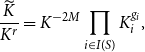 \begin{align} & \frac{\widetilde{K}}{K^r} = K^{-2M} \prod _{i \in I(S)} K_i^{g_i}, \end{align}
 \begin{align} & \frac{\mathrm{Cat}_{n-d_\pm }}{\mathrm{Cat}_{n-r \ell (S) + r c_\pm }} \sim 4^{-d_\pm +r(\ell (S)-c_\pm )} = 4^{2M(\ell (S)-c_\pm ) - \sum _{i \in I(S)} (\ell _i - c_\pm (i)) g_i}. \end{align}
and thus, from (4.41) and (4.12), recalling that $\sum _{i\in I(S)}g_i=M$
,
$\sum _{i\in I(S)}g_i=M$
,
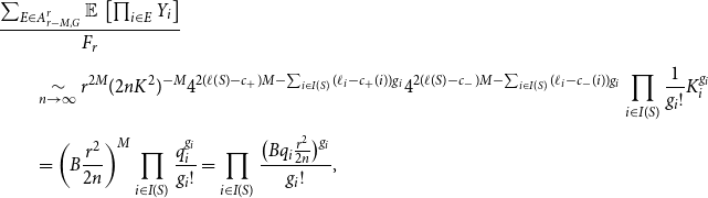 \begin{align} &\frac{\sum _{E \in A^r_{r-M, G}} \operatorname{\mathbb E}{}\left [ \prod _{i \in E} Y_i \right ]}{F_r} \\[5pt] \notag &\qquad \underset{n \rightarrow \infty }{\sim } r^{2M} (2nK^2)^{-M} 4^{2(\ell (S)-c_+)M - \sum _{i \in I(S)} (\ell _i - c_+(i))g_i} 4^{2(\ell (S)-c_-)M - \sum _{i \in I(S)} (\ell _i - c_-(i))g_i} \prod _{i \in I(S)} \frac{1}{g_i!} K_i^{g_i} \\[5pt] \notag &\qquad = \left ( B \frac{r^2}{2n} \right )^M \prod _{i \in I(S)} \frac{q_i^{g_i}}{g_i!} = \prod _{i \in I(S)} \frac{\bigl (Bq_i\frac{r^2}{2n}\bigr )^{g_i}}{g_i!}, \end{align}
where
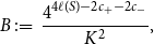 \begin{align} B&\;:\!=\;\frac{4^{4\ell (S)-2c_+-2c_-}}{K^2}, \end{align}
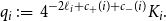 \begin{align} q_i&\;:\!=\;4^{-2\ell _i+c_+(i)+c_-(i)}K_i. \end{align}
The set $A^r_{r-M}(1,2)$
defined in Lemma 4.5(iii) is the union of
$A^r_{r-M}(1,2)$
defined in Lemma 4.5(iii) is the union of $A^{r}_{r-M,G}$
over all
$A^{r}_{r-M,G}$
over all $G$
with sum
$G$
with sum $M$
. Hence, (4.49) implies, noting that there is only a finite number of such
$M$
. Hence, (4.49) implies, noting that there is only a finite number of such $G$
,
$G$
,
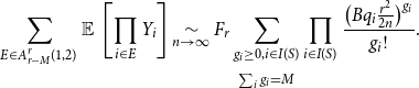 \begin{align} \sum _{E \in A^r_{r-M}(1,2)} \operatorname{\mathbb E}{}\left [ \prod _{i \in E} Y_i \right ] \underset{n \rightarrow \infty }{\sim } F_r \sum _{\substack{g_i\ge 0, i\in I(S)\\[5pt] \sum _i g_i=M}} \prod _{i \in I(S)} \frac{\bigl (Bq_i\frac{r^2}{2n}\bigr )^{g_i}}{g_i!} . \end{align}
The result (4.39) now follows from (4.52) and (4.16), using $Bq_i=b_i$
.
$Bq_i=b_i$
.
Proof of Theorem
1.2 for weak shapes. Let $r\to \infty$
with
$r\to \infty$
with $r\le \eta \sqrt n$
, where
$r\le \eta \sqrt n$
, where $\eta$
is as in Proposition 4.6.
$\eta$
is as in Proposition 4.6.
We may sum (4.39) over all $M\ge 0$
(with
$M\ge 0$
(with $A^r_{r-M}\;:\!=\;\emptyset$
for
$A^r_{r-M}\;:\!=\;\emptyset$
for $M\gt r$
), since Proposition 4.6 shows that we may approximate the sum by a finite sum with a fixed number of terms. Consequently, recalling (4.17),
$M\gt r$
), since Proposition 4.6 shows that we may approximate the sum by a finite sum with a fixed number of terms. Consequently, recalling (4.17),
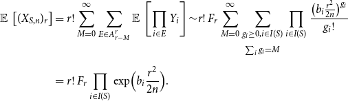 \begin{align} \operatorname{\mathbb E}{}\left [ (X_{S,n})_r \right ] &=r!\sum _{M=0}^\infty \sum _{E \in A^r_{r-M}} \operatorname{\mathbb E}{}\left [ \prod _{i \in E} Y_i \right ]{\sim } r!\,F_r \sum _{M=0}^\infty \sum _{\substack{g_i\ge 0, i\in I(S)\\[5pt] \sum _i g_i=M}} \prod _{i \in I(S)} \frac{\bigl (b_i\frac{r^2}{2n}\bigr )^{g_i}}{g_i!} \\[5pt] \notag & =r!\,F_r\prod _{i \in I(S)} \exp \Bigl (b_i\frac{r^2}{2n}\Bigr ) . \end{align}
By Lemmas 2.2 and 2.3, (4.12) implies (similarly to [4.5])
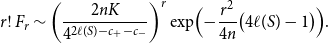 \begin{align} r!\,F_r\sim \left ( \frac{2n K}{4^{2\ell (S)-c_+-c_-}} \right )^r \exp \Bigl (-\frac{r^2}{4n}\bigl (4\ell (S)-1\bigr )\Bigr ). \end{align}
Finally, (4.53) and (4.54) yield, for $r\to \infty$
with
$r\to \infty$
with $r\le \eta \sqrt n$
,
$r\le \eta \sqrt n$
,
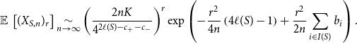 \begin{align} \operatorname{\mathbb E}{}\left [(X_{S,n})_r\right ] \underset{n \rightarrow \infty }{\sim } \left ( \frac{2n K}{4^{2\ell (S)-c_+-c_-}} \right )^r \exp \left ( -\frac{r^2}{4n} \left ( 4\ell (S)-1 \right ) + \frac{r^2}{2n}\sum _{i \in I(S)} b_i \right ). \end{align}
This is (2.2), with
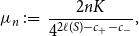 \begin{align} \mu _n&\;:\!=\;\frac{2n K}{4^{2\ell (S)-c_+-c_-}}, \end{align}
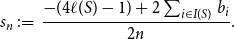 \begin{align} s_n&\;:\!=\;\frac{-(4\ell (S)-1)+2\sum _{i\in I(S)}b_i}{2n}. \end{align}
In particular, (2.2) thus holds for $r=r(n)$
with
$r=r(n)$
with $\frac{\eta }2\sqrt n \le r \le \eta \sqrt n$
; as noted in Section 2.1, it then automatically holds uniformly in this range. Furthermore,
$\frac{\eta }2\sqrt n \le r \le \eta \sqrt n$
; as noted in Section 2.1, it then automatically holds uniformly in this range. Furthermore,
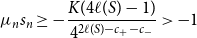 \begin{align} \mu _ns_n\ge -\frac{K (4\ell (S)-1) }{4^{2\ell (S)-c_+-c_-} }\gt -1 \end{align}
by Lemma 4.3, and we have again $\mu _n=\Theta (n)$
and
$\mu _n=\Theta (n)$
and $\sigma _n=\Theta (\sqrt n)$
. It follows that Theorem 2.1 applies in this case too, which yields (1.2).
$\sigma _n=\Theta (\sqrt n)$
. It follows that Theorem 2.1 applies in this case too, which yields (1.2).
 \begin{align} \sigma ^2_S=\frac{2 K}{4^{2\ell (S)-c_+-c_-}} \Bigl (1+\frac{ K}{4^{2\ell (S)-c_+-c_-}}\Bigl (1-4\ell (S)+2\sum _{i\in I(S)}b_i\Bigr ) \Bigr ), \end{align}
with $b_i$
given by (4.40). Note that this formula holds also for strong shapes (when
$b_i$
given by (4.40). Note that this formula holds also for strong shapes (when $I(S)=\emptyset$
) by (4.11).
$I(S)=\emptyset$
) by (4.11).
5. Open problems
We list here some open problems concerning possible extensions of our results.
-
1. It seems possible to extend the arguments above to joint factorial moments
(5.1)for several shapes
\begin{align} \operatorname{\mathbb E}{}\bigl [(X_{S_1,n})_{r_1}\dotsm (X_{S_k,n})_{r_k}\bigr ] \end{align}
$S_1,\dots,S_k$
and then obtain a multivariate version of Theorem 1.2 using a multivariate version of Gao and Wormald’s theorem [Reference Ojeda, Holmgren and Janson3], [Reference Wormald8]. However, we have not checked the details. Such a multivariate theorem would immediately imply, for example, a central limit theorem for the number of components of a given half-length.
-
2. Considering shapes that are similar, can we obtain a central limit theorem for the number of components that only cross the horizontal axis twice (i.e. the support has size 2, but the half-length is arbitrary)?
-
3. Is is true, as Kargin [Reference Kargin6] has conjectured, that the total number of components is asymptotically normal?


 Open access