







1. Introduction
Turbulence involves energy transfer across a wide range of scales and is important for many applications, such as combustion (Ertesvåg & Magnussen Reference Ertesvåg and Magnussen2000), ocean engineering (Hasselmann, Munk & MacDonald Reference Hasselmann, Munk and MacDonald1963) and the Earth's climate (Richardson Reference Richardson1922). It is generally understood that energy is transferred from large scales to small scales, known as the forward cascade (Richardson Reference Richardson1922; Kolmogorov Reference Kolmogorov1941). But an inverse cascade in which energy is transferred from small scales to large scales also occurs (Domaradzki et al. Reference Domaradzki, Liu, Härtel and Kleiser1994; Dunn & Morrison Reference Dunn and Morrison2003; Cimarelli, De Angelis & Casciola Reference Cimarelli, De Angelis and Casciola2013; Cimarelli et al. Reference Cimarelli, De Angelis, Jimenez and Casciola2016). Both forward and inverse cascades are involved in vortex regeneration in the self-sustaining process for wall turbulence (Hamilton, Kim & Waleffe Reference Hamilton, Kim and Waleffe1995; Waleffe Reference Waleffe1997). In turbulence modelling and simulation, failure to consider backscatter can result in inaccurate large-eddy simulations (LES) (Piomelli et al. Reference Piomelli, Cabot, Moin and Lee1991; Härtel et al. Reference Härtel, Kleiser, Unger and Friedrich1994; Cimarelli & De Angelis Reference Cimarelli and De Angelis2014). The above considerations are all dictated by the physics of the energy cascade across scales in wall-bounded turbulent flows.
This energy cascade can be viewed in either physical space or Fourier space. In physical space, the energy cascade is characterised by high spatio-temporal intermittency (Meneveau & Sreenivasan Reference Meneveau and Sreenivasan1991). In Fourier space, for flow geometries (such as channels, pipes, boundary layers) with at least one homogeneous spatial dimension, the energy cascade can be interpreted as energy redistributed among different Fourier modes, described by the nonlinear energy transfer term in the spectral turbulent kinetic energy (sTKE) equation (Tennekes & Lumley Reference Tennekes and Lumley1972; Pope Reference Pope2000). Here, a mode refers to scales with a particular wavelength in the homogeneous direction. The nonlinear energy transfer term in the spectral energy budget represents the net energy received by a particular mode from all other modes through nonlinear interactions since the term is a convolution of all wavenumber-compatible triadic interactions. Triadic interaction refers to the energy transfer among three modes whose wavenumbers satisfy  $\boldsymbol {k}+\boldsymbol {p}+\boldsymbol {q}=\boldsymbol {0}$ (Domaradzki & Rogallo Reference Domaradzki and Rogallo1990; Domaradzki Reference Domaradzki1992; Waleffe Reference Waleffe1992; Domaradzki et al. Reference Domaradzki, Liu, Härtel and Kleiser1994). However, we merely know the net energy transfer for each Fourier mode, not the detailed contributions to this net value from the nonlinear energy transfer term, because the convolution hides the individual triadic interactions.
Compared to homogeneous isotropic turbulence, only a few studies have explored the triadic interactions of nonlinear energy transfer for channel flows (Domaradzki et al. Reference Domaradzki, Liu, Härtel and Kleiser1994; Webber, Handler & Sirovich Reference Webber, Handler and Sirovich2002; Cho, Hwang & Choi Reference Cho, Hwang and Choi2018; Karban et al. Reference Karban, Martini, Cavalieri and Jordan2023). A single wavenumber triad could be interpreted as energy transfer from a source mode to a recipient mode via an advective mode (Domaradzki & Rogallo Reference Domaradzki and Rogallo1990; Smyth Reference Smyth1992; Webber et al. Reference Webber, Handler and Sirovich2002; Alexakis, Mininni & Pouquet Reference Alexakis, Mininni and Pouquet2005; Jin, Symon & Illingworth Reference Jin, Symon and Illingworth2021). To gain more insight into the energy cascade in channel flows, we expand the convolution of the nonlinear energy transfer term in streamwise–spanwise wavenumber space. Following this, we formulate a variable  $\hat {M}_{(s_x,s_y)(k_x,k_y)}$ (defined in § 2.3) that represents mode-to-mode nonlinear energy transfer in streamwise–spanwise wavenumber space. Compared to the convolution term, which gives us only the net energy transfer for a specific Fourier mode, with this variable, we are able to quantify the energy transfer between any two Fourier modes.
We use this four-dimensional variable  $\hat {M}_{(s_x,s_y)(k_x,k_y)}$ (one source mode and one recipient mode, with each mode consisting of a streamwise wavenumber and a spanwise wavenumber) to explore three things using direct numerical simulations (DNS) datasets at $Re_{\tau }=180$ and $590$. First, since the nonlinear energy transfer term in the sTKE equations could give us only one value representing the net energy transfer for each mode previously, we use this new variable $\hat {M}_{(s_x,s_y)(k_x,k_y)}$ to obtain two additional values quantifying the net energy transfer gain and loss due to nonlinear interactions for each mode. Second, we investigate the nonlinear energy transfer budgets for three types of modes. Similar to Jovanović & Bamieh (Reference Jovanović and Bamieh2005), each type of mode indicates a specific region in the streamwise–spanwise wavenumber space. Third, we apply a cutoff wavenumber filter to divide all the scales in the DNS into large and small scales. In the spirit of LES, the large scales are treated as resolved scales, while the small scales are treated as subgrid scales. We quantify the forward cascade and inverse cascade between resolved and subgrid scales. We further compare the net forward cascade calculated using $\hat {M}$ with the forward cascade calculated using the Smagorinsky eddy viscosity. The similarities and differences between $Re_{\tau }=180$ and $590$ are discussed. It is worth noting that we integrate energy transfer in the wall-normal direction and over time to obtain $\hat {M}$. Although $\hat {M}$ provides information in the streamwise–spanwise wavenumber space, it does not capture wall-normal-dependent and time-dependent information.
This paper is organised as follows. In § 2, the equations for the sTKE budget and variable  $\hat {M}_{(s_x,s_y)(k_x,k_y)}$ representing mode-to-mode nonlinear energy transfer are derived. The DNS datasets are described in § 3. Section 4 presents the results. Specifically, § 4.1 revisits the previous study from Symon, Illingworth & Marusic (Reference Symon, Illingworth and Marusic2021) about the wall-normal integrated spectral energy transfer budget; § 4.2 uses two examples to interpret variable $\hat {M}$ and to illustrate energy transfer pathways; § 4.3 presents the positive and negative nonlinear energy transfer spectra; § 4.4 investigates the nonlinear energy transfer for three types of modes; and § 4.5 quantifies the forward cascade and inverse cascade between resolved scales and subgrid scales in the spirit of LES. Conclusions are drawn in § 5.
2. Methods
In § 2.1, we describe the governing equations for plane Poiseuille flow and their non-dimensionalisation. Then an introduction to the sTKE equation integrated across the channel height is presented in § 2.2. In § 2.3, we introduce a four-dimensional variable quantifying mode-to-mode nonlinear energy transfer and the pertinent properties.
2.1. Plane Poiseuille flow equations
Consider the non-dimensional incompressible Navier–Stokes equations for the fluctuation velocities after a decomposition  $\mathcal {U}_i = U_i + u_i$, where $\mathcal {U}_i$, $U_i$ and $u_i$ represent the instantaneous velocity, streamwise–spanwise-averaged velocity and fluctuation velocity, respectively:
 \begin{equation} \left.\begin{gathered} \frac{\partial u_i}{\partial x_i} = 0, \\ \frac{\partial u_i}{\partial t} + u_j\,\frac{\partial U_i}{\partial x_j} + U_j\,\frac{\partial u_i}{\partial x_j} + \frac{\partial}{\partial x_j} (u_i u_j- \langle u_i u_j\rangle_{xy} ) ={-}\frac{\partial p}{\partial x_i} + \frac{1}{Re_{\tau}}\,\frac{\partial^2 u_i}{\partial x_j\,\partial x_j}, \end{gathered}\right\} \end{equation}
where the indices  $i=1,2,3$ represent the $x$ (streamwise), $y$ (spanwise) and $z$ (wall-normal) directions. The corresponding velocity components are denoted by $u$,
$u$,  $v$ and $w$. Pressure is denoted as $p$. Velocity scales are non-dimensionalised using the friction velocity $u_{\tau }$, length scales are non-dimensionalised using the channel half-height $h$, time scales are non-dimensionalised using $h/u_{\tau }$, and pressure is non-dimensionalised using $\rho u_{\tau }^2$, where $u_{\tau }=\sqrt {\tau _w/\rho }$, $\rho$ is the density, $\tau _w$ is the mean wall shear stress, and $u_{\tau }$ is the friction velocity. Then the friction Reynolds number $Re_{\tau } = hu_{\tau }/\nu$ is defined using $h$,
$h$,  $u_{\tau }$ and the kinematic viscosity $\nu$. Here, $\langle \, \rangle _{xy}$ means averaging in the streamwise and spanwise directions.
2.2. Spectral energy transfer budget
Owing to the periodic assumption in the streamwise and spanwise directions, we investigate energy transfer in two-dimensional streamwise–spanwise wavenumber space. We define the inner product  $\langle c_1,c_2 \rangle = \frac {1}{2} \int _{-1}^{1} c_1^* c_2 \,\mathrm {d} z$, where $c_1$ and $c_2$ are two complex vectors, and $^*$ denotes the complex conjugate. We use this inner product definition to represent the wall-normal integrated kinetic energy at mode $(k_x,k_y)$ (Reddy & Henningson Reference Reddy and Henningson1993; Domaradzki et al. Reference Domaradzki, Liu, Härtel and Kleiser1994):
 \begin{equation} \hat{E}(k_x,k_y) = \tfrac{1}{2} \langle \hat{u}^{(k_x,k_y)}, \hat{u}^{(k_x,k_y)} \rangle + \tfrac{1}{2} \langle \hat{v}^{(k_x,k_y)}, \hat{v}^{(k_x,k_y)} \rangle + \tfrac{1}{2} \langle \hat{w}^{(k_x,k_y)}, \hat{w}^{(k_x,k_y)} \rangle, \end{equation}
where  $k_x$ is the streamwise wavenumber, and $k_y$ is the spanwise wavenumber. The wavenumber is defined as $k = 2{\rm \pi} / \lambda$, where $\lambda$ is the wavelength. According to the non-dimensionalisation rule, wavenumbers $k_x$ and $k_y$ are scaled with the channel height $h$. Wavenumbers in viscous units are sometimes used: $k^+ = k \nu /h u_{\tau }$. The superscript refers to the individual Fourier mode under consideration: $\hat {u}^{(k_x,k_y)}$ is the Fourier coefficient of $u$ at wavenumber $(k_x,k_y)$.
The spectral energy transfer budget can be obtained by first taking Fourier transforms of (2.1) in the  $x$ and $y$ directions, and then multiplying by the conjugate mode $(\hat {u}_i^{(k_x,k_y)})^* = \hat {u}_i^{(-k_x,-k_y)}$. Then we integrate the energy transfer budget in the wall-normal direction and obtain (Symon et al. Reference Symon, Illingworth and Marusic2021)
 $$\begin{gather} \overline{\frac{\partial \hat{E}{(k_x , k_y)}}{\partial t}} = \underbrace{-\overline{\left\langle \hat{u}, \frac{\mathrm{d} U}{\mathrm{d} z}\,\hat{w}\right\rangle}}_{\hat{P}{(k_x , k_y)}} -\underbrace{\frac{1}{Re_{\tau}} \overline{\left\langle \widehat{\frac{\partial u_i}{\partial x_j}}, \widehat{\frac{\partial u_i}{\partial x_j}} \right\rangle}}_{\hat{D} (k_x , k_y)} \underbrace{{}- \overline{\left\langle \hat{u}_i, \widehat{\frac{\partial u_i u_j}{\partial x_j}} \right\rangle}}_{\hat{N}(k_x, k_y)}, \end{gather}$$
 $$\begin{gather}\hat{P}{(k_x, k_y)} - \hat{D}{(k_x , k_y)} + \hat{N}{(k_x , k_y)} =0, \end{gather}$$
with summation implied in the coordinate directions over the repeating index  $i$ or $j$. The angle brackets denote the inner product definition provided at the beginning of this section. This inner product involves integration in the wall-normal direction. The overbar denotes time-averaging. Equation (2.3a) describes the wall-normal integrated energy transfer balance for a single Fourier mode. The left-hand side is the time derivative of the turbulent kinetic energy for a single Fourier mode; $\hat {P}$ represents production, $-\hat {D}$ represents (pseudo) dissipation (Pope Reference Pope2000), and $\hat {N}$ represents the net nonlinear energy transfer (the net energy that mode $(k_x,k_y)$ receives through nonlinear interactions with all other modes). The size of an eddy corresponding to a given Fourier mode can be defined using the isotropic wall-parallel wavelength: $\lambda _I = 2{\rm \pi} /k_I$, where $k_I^2 = k_x^2 + k_y^2$ (Jiménez Reference Jiménez2018; Lee & Moser Reference Lee and Moser2019). For a statistically stationary flow, the left-hand side of (2.3a) is zero, meaning that the wall-normal integrated production, dissipation and net nonlinear energy transfer reach a balance for each mode, as shown in (2.3b). According to the normalisation described in § 2.1, the energy transfer terms ( $\hat {P}$, $\hat {D}$ and $\hat {N}$ in (2.3a)) are non-dimensionalised by $u_{\tau }^3/h$. Strictly speaking, production, dissipation and nonlinear energy transfer in (2.3a) are energy transfer rates because it is the kinetic energy variation rate on the left-hand side of (2.3a).
Throughout this paper, we use non-negative wavenumbers to describe a mode  $(k_x,k_y)$, where $k_x \geq 0$ and $k_y \geq 0$. Energy transfer at mode $(0,0)$ is zero because of the chosen decomposition of the velocities. The energy transfer at mode $(k_x,k_y)$ with $k_x > 0$ and $k_y > 0$ contains the contributions from the wavenumber pairs $(k_x,k_y)$, $(-k_x,-k_y)$, $(-k_x,k_y)$ and $(k_x,-k_y)$. For example, production at mode $(k_x,k_y)$ is equal to $\hat {P}(k_x,k_y)+\hat {P}(-k_x,k_y) + \mathrm {c.c.}$, where $\mathrm {c.c.}$ represents complex conjugate terms. The energy transfer at mode $(k_x,0)$ with $k_x > 0$ contains the contributions from the wavenumber pairs $(k_x,0)$ and $(-k_x,0)$. For example, production at mode $(k_x,0)$ is equal to $\hat {P}(k_x,0) + \mathrm {c.c.}$. The energy transfer at mode $(0,k_y)$ with $k_y > 0$ contains the contributions from the wavenumber pairs $(0,k_y)$ and $(0,-k_y)$. For example, production at mode $(0,k_y)$ is equal to $\hat {P}(0,k_y) + \mathrm {c.c.}$. Following this, the energy transfer terms $\hat {P},\hat {D},\hat {N}$ for each mode $(k_x,k_y)$ with $k_x\geq 0$, $k_y\geq 0$ are real numbers. The derivation of (2.3a) can be found in Pope (Reference Pope2000).
In (2.3a),  $\hat {N}(k_x,k_y)$ is conservative:
 \begin{equation} \int_{0}^{\infty} \int_{0}^{\infty} \hat{N}(k_x,k_y)\,\mathrm{d} k_x \,\mathrm{d} k_y = 0. \end{equation}
Equation (2.4) states that the sum of the net nonlinear energy transfer across all Fourier modes is zero. This implies that nonlinear energy transfer redistributes energy across scales without adding or removing energy overall. This can also be seen from the Reynolds–Orr equation: the only energy source for turbulence is production, and the only energy sink for turbulence is dissipation (Schmid & Henningson Reference Schmid and Henningson2001).
2.3. Mode-to-mode nonlinear energy transfer  $\hat {M}_{(s_x,s_y)(k_x,k_y)}$

On the right-hand side of (2.3a),  $\hat {N}(k_x,k_y)$ represents the net energy received by mode $(k_x,k_y)$ from nonlinear interactions between mode $(k_x,k_y)$ and all other modes, without giving information about the individual contributions to this net value. To illustrate, mode $(k_{x},k_{y})$ could potentially gain energy from mode $(s_{x1},s_{y1})$, lose energy to mode $(s_{x2},s_{y2})$, gain energy from mode $(s_{x3},s_{y3})$, lose energy to mode $(s_{x4},s_{y4})$, and so on. But those mode-to-mode nonlinear energy transfers are hidden because $\hat {N}$ represents a sum over all modes.
In (2.3a),  $\hat {N}(k_x,k_y)$ can be expressed as a convolution composed of all wavenumber-compatible triadic interactions:
 \begin{equation} \hat{N}(k_x,k_y) = \int_{0}^{\infty} \int_{0}^{\infty} \hat{M}_{(s_x,s_y)(k_x,k_y)}\,\mathrm{d} s_x \,\mathrm{d} s_y, \end{equation}
where
 \begin{equation} \hat{M}_{(s_x,s_y)(k_x,k_y)} ={-} \overline{\hat{u}_i^{({-}k_x,-k_y)}\, \hat{u}_j^{(k_x - s_x,k_y- s_y)}\,\widehat{\frac{\partial u_i}{\partial x_j}}^{(s_x,s_y)}}. \end{equation}
A single set of triadic interactions involving three distinct modes can be understood as the energy transferred nonlinearly from a source mode  $(s_x,s_y)$ to a recipient mode $(k_x,k_y)$ with the help of an advective mode $(k_x - s_x, k_y - s_y)$ (Domaradzki & Rogallo Reference Domaradzki and Rogallo1990; Smyth Reference Smyth1992; Webber et al. Reference Webber, Handler and Sirovich2002; Alexakis et al. Reference Alexakis, Mininni and Pouquet2005; Jin et al. Reference Jin, Symon and Illingworth2021; de Salis Young, Hao & Garcia-Mayoral Reference de Salis Young, Hao and Garcia-Mayoral2024). Here, $s_x$ is the streamwise wavenumber and $s_y$ is the spanwise wavenumber for another mode $(s_x,s_y)$ different from mode $(k_x,k_y)$. Thus the four-dimensional variable $\hat {M}_{(s_x,s_y)(k_x,k_y)}$ describes the energy transferred nonlinearly from one Fourier mode $(s_x,s_y)$ to another Fourier mode $(k_x,k_y)$. Compared to $\hat {N}$, $\hat {M}$ provides more detailed information about nonlinear energy transfer. However, it should be noted that $\hat {M}$ does not capture all details as $\hat {M}$ measures the time-averaged wall-normal-integrated energy transfer, condensing the information in the wall-normal direction and over time. Although the advective mode $(k_x-s_x,k_y-s_y)$ is one component of $\hat {M}$ (McKeon Reference McKeon2017; Lozano-Durán, Bae & Encinar Reference Lozano-Durán, Bae and Encinar2020; Bae, Lozano-Duran & McKeon Reference Bae, Lozano-Duran and McKeon2021; de Salis Young et al. Reference de Salis Young, Hao and Garcia-Mayoral2024), this paper focuses on the source mode $(s_x,s_y)$ and recipient mode $(k_x,k_y)$.
As mentioned before, we consider modes composed with non-negative wavenumbers. The full expressions for  $\hat {M}_{(s_x,s_y)(k_x,k_y)}$ with $s_x,s_y,k_x,k_y \geq 0$ are discussed in detail in Appendix A. Most result discussions in this paper centre on the mode-to-mode nonlinear energy transfer $\hat {M}$ in (2.6). For ease of reading, we sometimes omit the word ‘nonlinear’. Apart from production and dissipation, energy transfer, gaining energy and losing energy in the following discussions refer to $\hat {M}$ in (2.6) due to nonlinear interactions.
Furthermore,  $\hat {M}$, which represents wall-normal integrated energy transfer, satisfies the identities
 $$\begin{gather} \hat{M}_{(s_x,s_y)(k_x,k_y)} ={-} \hat{M}_{(k_x,k_y)(s_x,s_y)}, \end{gather}$$
 $$\begin{gather}\hat{M}_{(k_x,k_y)(k_x,k_y)} = 0. \end{gather}$$
Equation (2.7) states that the nonlinear energy transfer from mode  $(s_x,s_y)$ to mode $(k_x,k_y)$ is equal and opposite to the nonlinear energy transfer from mode $(k_x,k_y)$ to mode $(s_x,s_y)$. Equation (2.8) states that each mode transfers zero energy nonlinearly to itself. Equations (2.7) and (2.8) arise from the continuity equation and the boundary conditions at the walls (the proof is in Appendix B).
Here,  $\hat {P}$, $\hat {D}$, $\hat {N}$ and $\hat {M}$ represent densities of energy transfer per unit time and per unit volume.
3. Simulation parameters
The DNS are performed using a staggered-grid fourth-order finite-difference solver (Chung, Monty & Ooi Reference Chung, Monty and Ooi2014). Table 1 summarises the simulation parameters. For  $L_x = 2{\rm \pi}$ and $L_y={\rm \pi}$, the maximum wavenumbers resolved by the simulation are $k_x = \pm 55$, $k_y = \pm 110$ for $Re_{\tau } = 180$, and $k_x = \pm 191$, $k_y = \pm 382$ for $Re_{\tau } = 590$; the minimum wavenumbers are $k_x = \pm 1$, $k_y = \pm 2$ for both Reynolds numbers. The grids are evenly distributed in the streamwise and spanwise directions. In the wall-normal direction, the grid follows a Chebyshev distribution. The grid coordinate in the $z$ direction is $z=\cos ({n}/{N{\rm \pi} })$, $z \in [-1,1]$, where $n$ is an integer from $0$ to $n_z$ (in table 1), and $n_z$ is the total number of grid point in the $z$ direction.
Parameter setup of the DNS:  $L$ is domain length, $n$ is number of grid points, $\varDelta ^+$ is grid-spacing in viscous units, and $\Delta t$ is the simulation time step.

For  $Re_{\tau }=180$, the total simulation time is $20h/u_{\tau }$ with time step $0.002 h/u_{\tau }$; for $Re_{\tau }=590$, the total simulation time is $10h/u_{\tau }$ with time step $0.0002h/u_{\tau }$. Here, $h/u_{\tau }$ is used as the time unit for non-dimensionalisation. The time-averaged first- and second-order statistics of the present DNS data show good agreement with Moser, Kim & Mansour (Reference Moser, Kim and Mansour1999), as shown in figure 1.
Comparison between the DNS dataset represented by solid lines and the standard DNS dataset (Moser et al. Reference Moser, Kim and Mansour1999) represented by discrete markers: (a) mean streamwise velocity; (b) turbulence stresses. Here, blue indicates  $Re_{\tau }=180$, and black indicates $Re_{\tau }=590$.

4. Results
4.1. Energy transfer distributions
This subsection revisits the wall-normal integrated energy transfer for a single mode, as stated in (2.3a) (Symon et al. Reference Symon, Illingworth and Marusic2021). Different from Symon et al. (Reference Symon, Illingworth and Marusic2021), we use two full channel datasets, and visualise the premultiplied energy transfer spectra, as shown in figure 2. The relationship between wavenumber and wavelength is  $\lambda = 2{\rm \pi} /k$, where $\lambda$ refers to wavelength, and $k$ refers to wavenumber. We see that the wall-normal integrated production spectra $\hat {P}$ (figures 2a,d) show relatively $Re_{\tau }$-independent features at these two Reynolds numbers: their peaks are nearly aligned. For the wall-normal integrated dissipation spectra $\hat {D}$ (figures 2b,e), we see that there is a small peak shift towards a smaller streamwise wavelength from $Re_{\tau }=180$ to $Re_{\tau }=590$. The locations of the peaks are in line with the previous study that the production peak occurs at $\lambda _x^+ \approx 600$, $\lambda _y^+ \approx 100$ (at $z^+ \approx 15$), and the peak for dissipation caused by streamwise velocities occurs at $\lambda _x^+ \approx 200$, $\lambda _y^+ \approx 70$ (at $z^+ \approx 70$) (Lee & Moser Reference Lee and Moser2019). The energy transfer spectra integrated along the wall-normal height at $Re_{\tau }=180$ and $590$ do not show significant differences, primarily because of the short outer layers at low $Re_{\tau }$. The contribution from the large scales in the outer layer would become more significant as $Re_{\tau }$ increases (Hutchins & Marusic Reference Hutchins and Marusic2007; Lee & Moser Reference Lee and Moser2019). The Reynolds–Orr equation states that the energy source for turbulence is production, and the energy sink is dissipation (Schmid & Henningson Reference Schmid and Henningson2001). However, the energy source and sink are characterised by different structures, as large scales are responsible mainly for production and small scales are responsible mainly for dissipation. When viewed in terms of individual Fourier modes, (2.3a) states that the gap between production and dissipation is bridged by nonlinear energy transfer that is conservative, as shown in (2.4). As for the nonlinear energy transfer spectra $\hat {N}$ (figures 2c, f), we see the same streamwise forward cascade in which energy is transferred from large streamwise scales to small streamwise scales at $Re_{\tau }=180$ and $590$.
(a,d) Premultiplied production spectra  $k_x k_y \hat {P}$. (b,e) Premultiplied (negative) dissipation spectra $k_x k_y \hat {D}$. (c, f) Premultiplied nonlinear energy transfer spectra $k_x k_y \hat {N}$. Here, (a,b,c) $Re_{\tau }=180$ and (d,e, f) $Re_{\tau }=590$.

Recall that  $\hat {N}$ represents the net energy that one mode receives from all other modes through nonlinear interactions. Observing figures 2(c, f), we see that there is a band of modes near $\lambda _x^+ \approx 300$ with near-zero net energy transfer $\hat {N}(k_x,k_y) \approx 0$. However, $\hat {N}=0$ alone cannot distinguish these two possible cases: first, these modes do not participate in nonlinear interactions; second, these modes gain and lose approximately the same amount of energy, resulting in a near-zero energy transfer. Similarly, for modes for which $\hat {N} \neq 0$, $\hat {N}$ provides only the net energy transfer for one mode without giving the detailed budget. We see the same streamwise forward cascade at $Re_{\tau }=180$ and $590$ (figures 2c, f) by examining $\hat {N}$. However, it is not the only piece of information that we can obtain from the nonlinear interactions. In order to explore nonlinear interactions in more detail, we investigate the mode-to-mode nonlinear energy transfer using the variable $\hat {M}_{(s_x,s_y)(k_x,k_y)}$ defined in (2.6).
4.2. Energy transfer pathways
We first use two examples to interpret the introduced four-dimensional variable  $\hat {M}_{(s_x,s_y)(k_x,k_y)}$ that represents energy transferred nonlinearly from mode $(s_x,s_y)$ to mode $(k_x,k_y)$, as shown in (2.6) and Appendix A. For each example, we first choose a streamwise wavenumber and a spanwise wavenumber for mode $(k_x,k_y)$, which remains fixed. Then we vary the streamwise and spanwise wavenumbers for mode $(s_x,s_y)$. Both examples use the $Re_{\tau }=180$ dataset. First, $\hat {M}$ is visualised with linear axes because modes containing zero wavenumbers cannot be shown on a premultiplied energy spectrum. Second, the premultiplied spectrum $s_x s_y \hat {M}$ is shown.
For the first example, we choose to fix mode  $(0,6)$ corresponding to $(\lambda _x^+ = \infty, \lambda _y^+=188)$. This mode has significant production at $Re_{\tau }=180$, which means that this mode gains significant energy from the mean flow. We would like to understand how this streamwise-constant mode redistributes energy to other modes. Figure 3(a) shows $\hat {M}_{(s_x,s_y)(0,6)}$, which quantifies the energy that mode $(0,6)$ marked by the black cross gains from modes in pink and loses to modes in green. We see that apart from gaining energy from the wider mode $(0,4)$ (wider in the spanwise direction), it loses energy to all other modes, including the even wider mode $(0,2)$. The colour intensity tells us that local nonlinear energy transfer between mode $(0,6)$ and its neighbouring modes in Fourier space is strong (Brasseur & Wei Reference Brasseur and Wei1994; Domaradzki et al. Reference Domaradzki, Liu, Härtel and Kleiser1994; Cho et al. Reference Cho, Hwang and Choi2018). In particular, mode $(0,6)$ loses the most energy to the next smallest streamwise scales with $s_x=1$ outlined in orange, representing a forward energy cascade. This forward cascade can also be observed from the arrow in the premultiplied spectrum in figure 4(a). The direction of the arrow is determined by identifying which mode receives the most energy from mode $(0,6)$. In this case, mode $(0,6)$ loses the most energy to mode $(1,6)$, so the arrow points from mode $(0,6)$ to mode $(1,6)$. The length of the arrow is proportional to the magnitude of the energy transfer from mode $(0,6)$ to mode $(1,6)$.
Plots of (a)  $\hat {M}_{(s_x,s_y)(0,6)}$, where the black cross marks the fixed mode $(0,6)$, and (b) $\hat {M}_{(s_x,s_y)(1,6)}$, where the black cross marks the fixed mode $(1,6)$. Modes marked in orange boxes are used to illustrate the property stated in (2.7). The data are calculated for the $Re_{\tau }=180$ case.

(a) The premultiplied spectrum  $s_x s_y \hat {M}_{(s_x,s_y)(0,6)}$, where the black cross marks the fixed mode $(0,6)$ corresponding to $(\lambda _x^+,\lambda _y^+)=(\infty,188)$. (b) The premultiplied spectrum $s_x s_y \hat {M}_{(s_x,s_y)(1,6)}$, where the black cross marks the fixed mode $(1,6)$ corresponding to $(\lambda _x^+,\lambda _y^+)=(1130,188)$. (c) The premultiplied spectrum $s_x s_y \hat {M}_{(s_x,s_y)(3,6)}$, where the black cross marks the fixed mode $(3,6)$ corresponding to $(\lambda _x^+,\lambda _y^+)=(377,188)$. The arrow in each plot marks the dominant energy transfer direction.

For the second example, we choose to fix mode  $(1,6)$ corresponding to $(\lambda _x^+ = 1130, \lambda _y^+=188)$. Figure 3(b) shows $\hat {M}_{(s_x,s_y)(1,6)}$. From the first example, we see that mode $(0,6)$ loses the most energy to this mode $(1,6)$. The two modes highlighted in orange boxes in figures 3(a,b) have the same magnitude but opposite signs, respecting (2.7). We see the similar forward energy cascade in which mode $(1,6)$ gains energy from the next largest streamwise scale with $s_x=0$ and loses energy to the next smallest streamwise scale with $s_x=2$ but larger spanwise scale with $s_y=4$. In general, inspecting the spanwise wavenumbers, we observe that mode $(1,6)$ loses a significant amount of energy to scales with larger spanwise wavelengths ( $s_y<6$). This corresponds to a spanwise inverse energy cascade in which energy is transferred from small spanwise scales to large spanwise scales (Cimarelli et al. Reference Cimarelli, De Angelis and Casciola2013, Reference Cimarelli, De Angelis, Jimenez and Casciola2016; Cho et al. Reference Cho, Hwang and Choi2018), though this inverse spanwise energy cascade is not obvious from the arrow in the premultiplied spectrum in figure 4(b).
Since the two selected modes  $(0,6)$ and $(1,6)$ exhibit minimal energy gain, we further examine mode $(3,6)$, which has a smaller streamwise wavelength. Figure 4(c) displays the premultiplied spectrum for mode $(3,6)$. The results indicate that mode $(3,6)$ gains energy from larger streamwise scales in the pink-coloured region and loses energy to smaller streamwise scales in the green-coloured region, demonstrating a streamwise forward cascade. It is worth noting that mode $(3,6)$ loses energy to a wide range of smaller streamwise scales. The arrow indicates only the direction in which mode $(3,6)$ loses the most energy.
For each example, we obtain one dominant energy transfer pathway from the fixed mode  $(k_x,k_y)$ to the mode to which the fixed mode $(k_x,k_y)$ loses the most energy (as shown by the arrows in figure 4). We further sweep through a sufficient number of resolved modes as source modes, and identify their largest recipient modes. For each case, we plot an arrow pointing from the source mode to its corresponding largest recipient mode, with the length of the arrow proportional to the magnitude of the energy transfer. The path of the nonlinear energy transfer in streamwise–spanwise wavenumber space is shown in figure 5. For both $Re_{\tau }=180$ and $590$, we see that there are large left-pointing arrows corresponding to the forward streamwise energy cascade, and large bottom-pointing arrows corresponding to the forward spanwise energy cascade. It should be noted that each arrow in figure 5 illustrates only the dominant energy transfer pathway for each fixed $(k_x,k_y)$ case, without showing other less dominant energy transfer pathways. In addition, the energy transfer pathways describe only the statistical properties because the variable $\hat {M}$ is a time-averaged quantity (2.6).
Dominant energy transfer pathways: (a)  $Re_{\tau }=180$, (b) $Re_{\tau }=590$.

The two examples (figure 3) illustrate the quantification of mode-to-mode nonlinear energy transfer in streamwise–spanwise wavenumber space. For mode  $(0,6)$, we can further calculate how much energy mode $(0,6)$ gains in total due to nonlinear interactions by summing all the modes in pink in figure 3(a). Similarly, we can calculate how much energy mode $(0,6)$ loses in total due to nonlinear interactions by summing all the modes in green in figure 3(a). The next subsection aims to calculate the net energy transfer gain and loss due to nonlinear interactions for each mode in streamwise–spanwise wavenumber space.
4.3. Decomposition of net nonlinear energy transfer $\hat {N}$

With the introduced variable  $\hat {M}$ in (2.5), we can decompose $\hat {N}$ for a given mode $(k_x,k_y)$ into positive and negative contributions:
 $$\begin{gather} \hat{N}^+(k_x,k_y) = \int_{0}^{\infty} \int_{0}^{\infty} \hat{M}_{(s_x,s_y)(k_x,k_y)} \{\hat{M}>0\}\,\mathrm{d} s_x \,\mathrm{d} s_y, \end{gather}$$
 $$\begin{gather}\hat{N}^{-}(k_x,k_y) = \int_{0}^{\infty} \int_{0}^{\infty} \hat{M}_{(s_x,s_y)(k_x,k_y)} \{\hat{M}<0\} \,\mathrm{d} s_x \,\mathrm{d} s_y, \end{gather}$$
where  $\{\,\}$ is an indicator. An indicator is equal to $1$ when the argument is true, and $0$ when the argument is false. The positive energy transfer $\hat {N}^+$ quantifies the total energy that mode $(k_x,k_y)$ gains from other modes. The negative energy transfer $\hat {N}^-$ quantifies the total energy that mode $(k_x,k_y)$ loses to other modes. According to (2.5), these two variables are linked to the net energy transfer $\hat {N}$ by
 \begin{equation} \hat{N}(k_x,k_y) = \hat{N}^+(k_x,k_y) + \hat{N}^{-}(k_x,k_y). \end{equation}
The triadic interaction in the streamwise–spanwise wavenumber space enables this decomposition. However, it is important to note that  $\hat {N}^+$ and $\hat {N}^-$ do not provide a complete picture of energy gain and loss, as $\hat {M}$ is derived through wall-normal integration and time averaging.
Figure 6(a,b) quantify the energy transfer gain and loss for each mode at  $Re_{\tau } = 180$. We see the dual characteristic of nonlinear energy transfer that each mode acts as an energy source and energy recipient. The difference between the energy transfer gain and loss for each mode results in the net nonlinear energy transfer spectrum $\hat {N}$, as shown in figure 6(c) and respecting equation (4.2). Figure 6(c) is the same as figure 2(c) and figure 6( f) is the same as figure 2( f). We see that the mode marked by the black cross where $\hat {N} \approx 0$ in figure 6(c) has non-negligible net energy loss and net energy gain as observed in the corresponding locations in figure 6(a,b). This indicates that this mode gains and loses approximately equal amount of energy, resulting in near-zero net nonlinear energy transfer. The production and dissipation spectra show that large scales lose energy because they gain the most energy through production, while small scales gain energy to dissipate it. This results in intermediate scales with a net zero $\hat {N}$. The $\hat {N}^+$ and $\hat {N}^-$ spectra indicate that energy gain and loss transition ‘smoothly’ across scales for the Reynolds numbers considered. However, this is not necessarily true for high-Reynolds-number flows.
Decomposition of the net nonlinear energy transfer:  $\hat {N}^- + \hat {N}^+ = \hat {N}$. (a,d) Premultiplied negative nonlinear energy transfer spectra $k_x k_y \hat {N}^-$, where dashed lines mark the peak. (b,e) Premultiplied positive nonlinear energy transfer spectra $k_x k_y \hat {N}^+$, where dashed lines mark the peak, (c, f) Premultiplied net nonlinear energy transfer spectra $k_x k_y \hat {N}$. Here, (a–c) $Re_{\tau }=180$, and (d–f) $Re_{\tau }=590$. The black crosses in (a–c) mark a mode with $\hat {N} \approx 0$ for explanation purposes.

Now we answer the other question raised at the end of § 4.1. As mentioned previously, the net energy transfer spectra  $\hat {N}$ reveal the same streamwise forward cascade at $Re_{\tau }=180$ and $590$ (figures 6c, f). At $Re_{\tau }=180$, we see that the negative energy transfer spectrum $\hat {N}^-$ peak is at $\lambda _x^+ \approx 600$, $\lambda _y^+ \approx 100$, and the positive energy transfer spectrum $\hat {N}^+$ peak is at $\lambda _x^+ \approx 150$, $\lambda _y^+ \approx 70$, indicated by the white dashed lines in figures 6(a,b). This indicates that large streamwise scales lose the most energy, and small streamwise scales gain the most energy. Thus figures 6(a,b) illustrate the streamwise forward cascade, which aligns with the net energy transfer spectrum (figure 6c).
At  $Re_{\tau }=590$, we see that the negative energy transfer spectrum $\hat {N}^-$ peak is at $\lambda _x^+ \approx 200$, $\lambda _y^+ \approx 90$, and the positive energy transfer spectrum $\hat {N}^+$ peak is at $\lambda _x^+ \approx 150$, $\lambda _y^+ \approx 80$, indicated by the white dashed lines in figures 6(d,e). From $Re_{\tau }=180$ to $590$, there is a significant negative energy transfer spectrum peak shift to a much smaller $\lambda _x^+$. The spectra of $\hat {N}^+$ and $\hat {N}^-$ reveal the same streamwise forward cascade as $\hat {N}$, because of (4.2). The shift of $\hat {N}^-$ peak cannot be deduced directly from the production and dissipation spectra, because $\hat {N}^-$ is obtained through the triadic interaction. The reason for this shift remains unclear at this stage. Note that the above discussions are for the whole channel since $\hat {M}$ is wall-normal integrated nonlinear energy transfer that hides the nonlinear energy transfer in the wall-normal direction.
4.4. Nonlinear energy transfer of three specific modes
Linear analysis explains the energy amplification mechanisms of different modes (Schmid & Henningson Reference Schmid and Henningson2001; Jovanović & Bamieh Reference Jovanović and Bamieh2005), leaving the nonlinear part relatively unexplored. Since nonlinear energy transfer is conservative, the nonlinear energy transfer among different modes should be interpreted as energy redistribution. In this subsection, we use  $\hat {M}$ to investigate the energy redistribution of three different modes: streamwise-constant modes, oblique 2 : 1 modes and spanwise-constant modes.
Following Jovanović & Bamieh (Reference Jovanović and Bamieh2005), we define the nonlinear energy transfer of the streamwise-constant modes as
 \begin{equation} \hat{M}_{(s_x,s_y) (k_x=0)} = \sum_{k_x=0} \hat{M}_{(s_x,s_y)(k_x,k_y)}. \end{equation}
Oblique waves are characterised by  $k_x \approx O(1)$, $k_y \approx O(1)$. Considering the geometry of the channel box used in this study, we define the nonlinear energy transfer of the oblique 2 : 1 modes (where 2 : 1 refers to $L_x/L_y=2\,{:}\,1$) as
 \begin{equation} \hat{M}_{(s_x,s_y) (k_y=2k_x)} = \sum_{k_y=2k_x} \hat{M}_{(s_x,s_y)(k_x,k_y)}. \end{equation}
We define the nonlinear energy transfer of the spanwise-constant modes as
 \begin{equation} \hat{M}_{(s_x,s_y)(k_y=0)} = \sum_{k_y=0} \hat{M}_{(s_x,s_y)(k_x,k_y)}. \end{equation}
 Figure 7 shows the nonlinear energy transfer of the three different modes at  $Re_{\tau }=180$ and $590$. As for the interpretation of each subplot, the specific modes (indicated by the black crosses) gain energy from modes in pink, and lose energy to modes in green. We see that the streamwise-constant modes (figures 7a,d) lose energy to smaller streamwise scales ( $s_x>0$), exhibiting a streamwise forward cascade. This could be linked to streak breakdown which is one phase of the self-sustaining process. Due to the instability of long streamwise streaks, they break down into smaller streamwise streaks (Hamilton et al. Reference Hamilton, Kim and Waleffe1995). The breakdown of streamwise streaks has been observed both experimentally (Blackwelder & Eckelmann Reference Blackwelder and Eckelmann1979) and numerically (Hwang & Bengana Reference Hwang and Bengana2016). For the oblique 2 : 1 modes (figures 7b,e), we see that they generally gain energy from scales with larger aspect ratios $s_y / s_x$ (which is equivalent to $k_y/k_x$) (Symon et al. Reference Symon, Illingworth and Marusic2021), and lose energy to scales with smaller aspect ratios, exhibiting a transverse cascade (Lee & Moser Reference Lee and Moser2019; Symon et al. Reference Symon, Illingworth and Marusic2021). For the spanwise-constant modes (figures 7c, f), we see that they mainly gain energy from smaller spanwise scales, exhibiting a spanwise inverse cascade (Cimarelli et al. Reference Cimarelli, De Angelis and Casciola2013, Reference Cimarelli, De Angelis, Jimenez and Casciola2016; Cho et al. Reference Cho, Hwang and Choi2018). If we think of the streamwise-constant modes with infinite aspect ratio $s_y / s_x \to \infty$ and the spanwise-constant modes with zero aspect ratio $s_y / s_x \to 0$, then we could conclude that there exists energy transfer from scales with large aspect ratio to scales with small aspect ratio. In terms of the shapes of scales, this transverse cascade refers to energy transfer from streamwise-elongated scales to spanwise-elongated scales. It is also worth noting that the transverse cascade of the three modes is not substantially influenced by the Reynolds number for this range.
Plots of (a,d)  $\hat {M}_{(s_x,s_y)(k_x=0)}$, (b,e) $\hat {M}_{(s_x,s_y)(k_y=2k_x)}$, (c, f) $\hat {M}_{(s_x,s_y)(k_y=0)}$, visualised using discrete modes. Here, (a–c) $Re_{\tau } = 180$, and (d–f) $Re_{\tau } = 590$. Black crosses mark the modes of the investigated structures.

The above discussion tells us that the transverse energy cascade is related to  $s_y / s_x$ (which is equivalent to $k_y/k_x$). We can also visualise this same piece of information on a log-polar coordinate in which $s_y / s_x$ corresponds to a certain slope (Lee & Moser Reference Lee and Moser2019), as shown in figure 8. Following Lee & Moser (Reference Lee and Moser2019), $s_x^{\#} = \xi s_x / \sqrt {s_x^2+s_y^2}$, $s_y^{\#} = \xi s_y / \sqrt {s_x^2+s_y^2}$ and $\xi = \log (\sqrt {s_x^2+s_y^2}/k_{ref})$, with $k_{ref} = Re_{\tau } / 50\,000$. From figures 8(a,d), the streamwise-constant modes located on the $s_x^{\#}=0$ axis lose energy to other modes, corresponding to the finding that modes located on the $s_x^{\#}=0$ axis have significant net negative nonlinear energy transfer (Lee & Moser Reference Lee and Moser2019). From figures 8(b,e), the oblique 2 : 1 modes located on $s_y^{\#} = 2 s_x^{\#}$ gain energy from modes satisfying $s_y^{\#} > 2 s_x^{\#}$, and lose energy to modes satisfying $s_y^{\#} < 2 s _x^{\#}$, corresponding to the transverse cascade mentioned previously. From figures 8(c, f), the spanwise-constant modes located on the $s_y^{\#}=0$ axis mainly gain energy but also lose a small amount of energy. We see that one advantage of using log-polar premultiplied spectra over the traditional premultiplied spectra is that we can visualise modes that contain one zero wavenumber (either $s_x=0$ or $s_y=0$).
Log-polar premultiplied energy spectra (a,d)  $({(s_x^2+s_y^2)}/{\xi })\, \hat {M}_{(s_x,s_y)(k_x=0)}$, (b,e) $({(s_x^2+s_y^2)}/{\xi })\, \hat {M}_{(s_x,s_y)(k_y=2k_x)}$, (c, f) $({(s_x^2+s_y^2)}/{\xi })\, \hat {M}_{(s_x,s_y)(k_y=0)}$. Here, (a–c) $Re_{\tau } = 180$, and (d–f) $Re_{\tau } = 590$. Black crosses mark the modes of the investigated structures.

Note that the above discussion concerns only the nonlinear energy transfer as one component in the energy transfer balance (2.3a). One should not interpret this as saying that energy merely originates from the streamwise-constant modes, goes through the oblique 2 : 1 modes, and finally dissipates at the spanwise-constant modes. Equation (2.3a) gives the energy transfer budget for each mode. To evaluate the overall energy transfer balance comprehensively, we need to consider the production and dissipation as well. Motivated by § 4.3, we decompose the net nonlinear energy transfer of each mode into its positive and negative parts. According to (2.3a) and (4.2), for each mode, the energy transfer budget is
 \begin{equation} \hat{P} + \hat{D} + \hat{N}^+ + \hat{N}^- = 0. \end{equation}
The energy budgets (2.3a) for the three modes are shown in figure 9. For the streamwise-constant modes, they receive a large amount of energy from the mean flow through production, as seen from the blue bars, and they lose a large amount of energy nonlinearly to other modes, as seen from the purple bars. For the oblique 2 : 1 modes, apart from gaining energy from the mean flow and dissipating energy, they gain and lose energy nonlinearly through interacting with other modes, as seen from the purple and yellow bars. For the spanwise-constant modes, the only energy gain is through nonlinear energy transfer, as seen from the yellow bars. The streamwise-constant modes and the oblique 2 : 1 modes gain energy from the mean flow (positive production), while the spanwise-constant modes lose energy to the mean flow (negative production). Dissipation occurs for all three modes as seen from the red bars. Although the values are different at the two Reynolds numbers, different types of energy transfer show similar trends in the three modes.
Energy budgets for the streamwise-constant mode ( $k_x=0$), oblique 2 : 1 mode ( $k_y=2k_x$) and spanwise-constant mode ( $k_y=0$). Here, (a) $Re_{\tau }=180$, and (b) $Re_{\tau }=590$.

Having discussed the three types of modes, we proceed to discuss a certain type of structure. It has been found that streamwise-constant modes with spanwise wavelengths  $\lambda _y^+ \approx 100$ experience significant energy growth due to linear mechanisms (Pujals et al. Reference Pujals, García-Villalba, Cossu and Depardon2009; Hwang & Cossu Reference Hwang and Cossu2010). Using the variable $\hat {M}$, we can investigate the nonlinear energy transfer of this specific structure. We define the mode-to-mode nonlinear energy transfer of streamwise streaks with $\lambda _y^+ \approx 100$ as
 \begin{equation} \hat{M}_{(s_x,s_y) (streaks)} = \sum_{k_x=0,\lambda_y^+{\approx} 100} \hat{M}_{(s_x,s_y)(k_x,k_y)}. \end{equation}
 Figure 10 shows the log-polar premultiplied energy spectra of streamwise streaks at  $Re_{\tau }=180$ and $590$. According to the definition in (4.7), the discussed streamwise streaks have zero streamwise wavenumber $k_x=0$, corresponding to $s_x^{\#}=0$. The discussed streamwise streaks have spanwise wavelength $\lambda _y^+ \approx 100$, corresponding to $s_y^{\#}=3.49$. We see that the streamwise streaks mainly lose energy to smaller scales at $Re_{\tau }=180$ and $590$. The main difference from figures 8(a,d) is that the streamwise streaks receive a small amount of energy from large scales, as indicated by the pink colour.
Log-polar premultiplied energy spectra of streamwise streaks  $({(s_x^2 + s_y^2)}/{\xi })\, \hat {M}_{(s_x,s_y)(streaks)}$. Black crosses mark the modes satisfying $k_x=0$ and $\lambda _y^+ \approx 100$. Here, (a) $Re_{\tau }=180$, and (b) $Re_{\tau }=590$.

4.5. Forward cascade and inverse cascade
In this subsection, we use  $\hat {M}$ to quantify the forward and inverse cascades between the large scales and small scales in the spirit of LES. For channel flows, resolved scales could be set by modes belonging to a rectangular region determined by the conditions $k_x \leq k_{xC}$ and $k_y \leq k_{yC}$, where $k_{xC}$ and $k_{yC}$ are cutoff wavenumbers (Germano et al. Reference Germano, Piomelli, Moin and Cabot1991; Domaradzki et al. Reference Domaradzki, Liu, Härtel and Kleiser1994; Härtel et al. Reference Härtel, Kleiser, Unger and Friedrich1994). These cutoff wavenumbers are determined by the choice of a single variable $n_C$:
 \begin{equation} k_{xC} = \frac{2{\rm \pi} n_C}{L_x},\quad k_{yC} = \frac{2{\rm \pi} n_C}{L_y}. \end{equation}
One issue of subgrid-scale energy transfer modelling with eddy viscosity is that it assumes that the subgrid scales only dissipate energy and neglects the energy transferred from the subgrid scales to the resolved scales, also known as ‘backscatter’ (Piomelli et al. Reference Piomelli, Cabot, Moin and Lee1991). Figure 11 illustrates the two-way energy transfer between the resolved scales and subgrid scales. We aim to quantify the forward cascade and inverse cascade using mode-to-mode nonlinear energy transfer  $\hat {M}$.
A sketch illustrating the forward cascade and inverse cascade between the resolved-scale region  $\mathbb {R}$ marked in dark grey and the subgrid-scale region $\mathbb {S}$ marked in light grey. Region $\mathbb {R}$ contains the resolved scales, and region $\mathbb {S}$ contains the subgrid scales. Here, $k_{xC}$ and $k_{yC}$ are the cutoff wavenumbers, and $k_{xDNS}$ and $k_{yDNS}$ are the maximum wavenumbers resolved by DNS.

Recall that  $\hat {M}_{(s_x,s_y)(k_x,k_y)}$ represents energy transfer from mode $(s_x,s_y)$ to mode $(k_x,k_y)$. For the forward cascade, energy is transferred from the resolved scales in region $\mathbb {R}$ to the subgrid scales in region $\mathbb {S}$, as indicated by the solid arrow in figure 11. Similar to (4.1a) and (4.1b), for this forward cascade, we can calculate the energy lost by each mode (4.9b) in the resolved-scale region $\mathbb {R}$ and the energy gained by each mode (4.9a) in the subgrid-scale region $\mathbb {S}$:
 $$\begin{gather} \hat{N}^+_{F}(k_x,k_y,n_C) = \iint \hat{M}_{(s_x,s_y)(k_x,k_y)} \{\hat{M}>0, (s_x,s_y) \in \mathbb{R}, (k_x,k_y) \in \mathbb{S}\}\,\mathrm{d} s_x \,\mathrm{d} s_y, \end{gather}$$
 $$\begin{gather}\hat{N}^{-}_{F}(k_x,k_y,n_C) = \iint \hat{M}_{(s_x,s_y)(k_x,k_y)}\{\hat{M}<0, (s_x,s_y) \in \mathbb{S}, (k_x,k_y) \in \mathbb{R}\} \,\mathrm{d} s_x \,\mathrm{d} s_y. \end{gather}$$
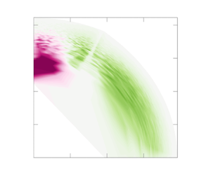
 Figure 12 shows an example of the forward cascade from the resolved scales to the subgrid scales at  $Re_{\tau }=180$. The choice of cutoff wavenumber $n_C=5$ corresponds to the filtering width $\varDelta _i$ satisfying $\varDelta _i \approx 5 \Delta x_i$ ( $i=1,2$) at $Re_{\tau }=180$. Figure 12(a) shows that streamwise-elongated modes with large $k_y/k_x$ in region $\mathbb {R}$ lose the most energy. Figure 12(b) shows that modes gaining energy in region $\mathbb {S}$ do not show significant preference with respect to $k_y/k_x$.
An example of the forward cascade, where  $n_C=5$ corresponds to $(\lambda _x^+ = 226, \lambda _y^+= 113)$ at $Re_{\tau }=180$: (a) $\hat {N}^{-}_{F}(k_x,k_y,5)$ shows the energy lost by resolved scales in region $\mathbb {R}$; (b) $\hat {N}^+_{F}(k_x,k_y,5)$ shows the energy gained by subgrid scales in region $\mathbb {S}$. Dashed lines mark the boundary between the resolved-scale region $\mathbb {R}$ and the subgrid-scale region $\mathbb {S}$. Note that the maximum wavenumbers in this figure are not the maximum wavenumbers resolved in the DNS.

For the inverse cascade, energy is transferred from the subgrid scales in region  $\mathbb {S}$ to the resolved scales in region $\mathbb {R}$, as indicated by the dashed-line arrow in figure 11. Similar to (4.1a) and (4.1b), for this inverse cascade, we can calculate the energy gained by each mode (4.10a) in the resolved-scale region $\mathbb {R}$, and the energy lost by each mode (4.10b) in the subgrid-scale region $\mathbb {S}$:
 $$\begin{gather} \hat{N}^+_{I}(k_x,k_y,n_C) = \iint \hat{M}_{(s_x,s_y)(k_x,k_y)} \{\hat{M}>0, (s_x,s_y) \in \mathbb{S}, (k_x,k_y) \in \mathbb{R}\} \, \mathrm{d} s_x \,\mathrm{d} s_y, \end{gather}$$
 $$\begin{gather}\hat{N}^{-}_{I}(k_x,k_y,n_C) = \iint \hat{M}_{(s_x,s_y)(k_x,k_y)} \{\hat{M}<0, (s_x,s_y) \in \mathbb{R}, (k_x,k_y) \in \mathbb{S}\} \,\mathrm{d} s_x \,\mathrm{d} s_y. \end{gather}$$
 Figure 13 shows an example of the inverse cascade from the subgrid scales to the resolved scales at  $Re_{\tau }=180$. Figure 13(a) shows the asymmetry of modes losing energy in region $\mathbb {S}$: only streamwise elongated modes with large $k_y/k_x$ lose energy. Figure 13(b) shows that modes gaining energy in region $\mathbb {R}$ do not show significant preference with respect to $k_y/k_x$.
Inverse cascade example:  $n_C=5$ ( $\lambda _x^+ = 226$, $\lambda _y^+= 113$) at $Re_{\tau }=180$. Here, (a) $\hat {N}^{-}_{I}(k_x,k_y,5)$ shows how subgrid scales in region $\mathbb {S}$ lose energy; (b) $\hat {N}^+_{I}(k_x,k_y,5)$ shows how resolved scales in region $\mathbb {R}$ gain energy.

We further quantify the forward cascade and inverse cascade between the resolved scales and subgrid scales determined by  $n_C$:
 $$\begin{gather} N_{F}(n_C) = \iint_{\mathbb{S}} \hat{N}^+_{F} \,\mathrm{d} k_x \,\mathrm{d} k_y \overset{(2.7)}={-}\iint_{\mathbb{R}} \hat{N}^{-}_{F} \, \mathrm{d} k_x \,\mathrm{d} k_y, \end{gather}$$
 $$\begin{gather}N_{I}(n_C) = \iint_{\mathbb{R}} \hat{N}^+_{I} \,\mathrm{d} k_x \,\mathrm{d} k_y \overset{(2.7)}={-}\iint_{\mathbb{S}} \hat{N}^{-}_{I} \, \mathrm{d} k_x \,\mathrm{d} k_y. \end{gather}$$
 The forward cascade and inverse cascade calculated using (4.11) and (4.12) for  $Re_{\tau }=180$ and $590$ are shown in figure 14. A general criterion for LES is to resolve a sufficient amount of large scales that should contain 80 % of the total kinetic energy (Pope Reference Pope2000). By checking the DNS datasets, we know that scales with $\lambda _{x}^+ = 2 \lambda _{y}^+ >162$ need to be resolved at $Re_{\tau }=180$, and scales with $\lambda _{x}^+ = 2 \lambda _{y}^+ >232$ need to be resolved at $Re_{\tau }=590$. Therefore, we need to consider the energy transfer when the cutoff wavelengths satisfy $\lambda _{xC}^+ = 2 \lambda _{yC}^+ <162$ at $Re_{\tau }=180$, and $\lambda _{xC}^+ = 2 \lambda _{yC}^+ <232$ at $Re_{\tau }=590$. We see that the forward cascade is at least four times larger than the inverse cascade when $\lambda _{xC}^+<250$, indicating that the net energy transfer is from the resolved scales to the subgrid scales, shown by the solid lines. This justifies why eddy viscosity considering only the forward cascade is used in LES (Pope Reference Pope2000). The net forward cascade from resolved scales to subgrid scales could also be expected from figure 2. Large scales are mainly responsible for production, and small scales are mainly responsible for dissipation. The imbalance between production and dissipation in terms of each scale results in the net forward energy cascade. However, the inverse cascade is not negligible when $\lambda _{xC}^+>100$, so the negligence of it has been proposed as a source of inaccuracy in LES (Anderson & Domaradzki Reference Anderson and Domaradzki2012; Cimarelli & De Angelis Reference Cimarelli and De Angelis2014).
Quantification of the energy transfer between the resolved scales and subgrid scales: (a) cutoff wavelengths are scaled in inner units; (b) cutoff wavelengths are scaled in outer units. Dashed lines indicate forward cascade  $N_{F}$; dotted lines indicate inverse cascade $N_{I}$; solid lines indicate net energy cascade $N_{F}-N_{I}$. Blue indicates $Re_{\tau }=180$; black indicates $Re_{\tau }=590$.

When interpreting figure 14, two things should be noted. First, the results would be different if the aspect ratio between the streamwise and spanwise cutoff wavenumbers  $k_{xC} / k_{yC} = \frac {1}{2}$ were changed. Second, the above results represent only the wall-normal integrated forward and inverse cascades. Due to the inhomogeneity in the wall-normal direction of wall-bounded flows, the forward cascade and inverse cascade would vary with wall-normal height.
Now we compare the energy cascade calculated using  $\hat {M}$ with the eddy viscosity method. The forward cascade from the resolved scales to the subgrid scales $N_{\nu }$ can be calculated using the linear eddy viscosity model (Pope Reference Pope2000)
 \begin{equation} N_{\nu} = \nu \tilde{S}^2, \end{equation}
where  $\nu$ is the eddy viscosity, $\tilde {S}$ is the characteristic filtered rate of strain $\tilde {S} = (2 \tilde {S}_{ij} \tilde {S}_{ij})^{{1}/{2}}$, $\tilde {S}_{ij}$ is the filtered rate-of-strain tensor $\tilde {S}_{ij} = \frac {1}{2} ({\partial \tilde {u}_i}/{\partial x_j} + {\partial \tilde {u}_j}/{\partial x_i})$, and $\tilde {u}_i$ is the filtered velocity of the resolved scales.
We can use the Smagorinsky eddy viscosity (Smagorinsky Reference Smagorinsky1963)
 \begin{equation} \nu = (C_s D_z \varDelta)^2 \tilde{S}, \end{equation}
where  $C_s$ is the Smagorinsky coefficient, set to be $C_s=0.067$ (Moin & Kim Reference Moin and Kim1982), and $D_z$ is the damping function that accounts for low-Reynolds-number subgrid-scale stress near the wall, set to be $D_z = 1-\exp (-z^+/25)$ (Moin & Kim Reference Moin and Kim1982). Since we do not apply filtering in the wall-normal direction, the characteristic length scale of the largest subgrid-scale eddies $\varDelta$ is set to be $\varDelta = (\varDelta _1 \varDelta _2)^{{1}/{2}}$. After we have obtained the filtered velocity fields $\tilde {u}_i$ using the cutoff wavenumbers (4.8a,b) in Fourier space, we calculate the forward cascade $N_{\nu }$ in (4.13) and the Smagorinsky eddy viscosity $\nu$ in (4.14) directly in physical space.
Figure 15 shows the forward cascades from the resolved scales to subgrid scales predicted by the eddy viscosity (4.14) at  $Re_{\tau }=180$ and $590$. We see that the forward cascade at $Re_{\tau }=590$ is approximately 20 times higher than the forward cascade at $Re_{\tau }=180$. We do not put the forward cascades predicted from (4.14) and from $\hat {M}$ on the same figure because they differ in magnitude substantially. Nevertheless, both the eddy viscosity (4.14) and $\hat {M}$ are able to predict the forward cascades with respect to cutoff wavelengths with the same shape. The forward cascade predicted by the eddy viscosity (4.14) first increases as the cutoff wavelengths ( $\lambda _{xC}$ and $\lambda _{yC}$) decrease, and then decreases to zero as the cutoff wavelengths approach the DNS grid sizes, aligning with the trends in figure 14. The substantial mismatch in magnitude between the eddy viscosity (4.14) and $\hat {M}$ is that $\hat {M}$ represents the wall-normal integrated energy transfer and is a time-averaged variable. Statistics of energy transfer has been averaged out in the wall-normal direction and the time domain, which could be more prominent at $Re_{\tau }=590$. That is the main reason why $N_F-N_I$ in figure 14 is substantially smaller than $N_{\nu }$ in figure 15. Nevertheless, $\hat {M}$ could be extended to include the wall-normal coordinate, and $N_F-N_I$ can be calculated at each wall-normal height before being time and wall-normal averaged.
Forward cascade  $N_{\nu }$ predicted by the eddy viscosity (4.14) in (a) inner units, (b) outer units. Blue indicates $Re_{\tau }=180$, left-hand axis; black indicates $Re_{\tau }=590$, right-hand axis.

5. Conclusions and outlook
We investigate nonlinear energy transfer in turbulent channel flow in Fourier space at  $Re_{\tau }=180$ and $590$. We introduce a four-dimensional variable $\hat {M}_{(s_x,s_y)(k_x,k_y)}$ that describes the nonlinear energy transfer between any two modes in streamwise–spanwise wavenumber space, by analysing the individual triadic interactions of the nonlinear energy transfer term in the spectral turbulent kinetic energy equation.
We use this variable to explore three things. First, we decompose the net nonlinear energy transfer  $\hat {N}$ into its positive and negative contributions: $\hat {N}^+$ and $\hat {N}^-$. This allows us to separately quantify the total energy gained and total energy lost by each mode. Second, we investigate the nonlinear energy transfer of three specific modes. We observe that there exists energy transfer from streamwise-elongated structures to spanwise-elongated structures, and that this transverse cascade is characterised by the aspect ratio $k_y/k_x$. Third, we quantify the forward cascade and inverse cascade between the resolved scales and subgrid scales in the spirit of LES. For both Reynolds numbers considered, the forward cascade is significantly larger than the inverse cascade when $\lambda _{xC}^+<250$, justifying why eddy viscosity considers only the forward cascade used in LES. However, the inverse cascade is not negligible when $\lambda _{xC}^+>100$. We also compare the energy cascade calculated using $\hat {M}$ with the Smagorinsky eddy viscosity. The forward cascades calculated from the two methods show a substantial deviation in magnitude and a similar trend with respect to the cutoff wavelengths.
The pathways illustrated by  $\hat {M}$ represent a nonlinear energy transfer network in two-dimensional Fourier space (Gürcan, Li & Morel Reference Gürcan, Li and Morel2020). A promising area for future work would be to extend mode-to-mode nonlinear energy transfer $\hat {M}_{(s_x,s_y)(k_x,k_y)}$ to include another dimension, the wall-normal coordinate, to investigate the details of mode-to-mode nonlinear energy transfer at any wall-normal height.
Funding
This research was supported by the University of Melbourne's Research Computing Services and the Petascale Campus Initiative.
Declaration of interests
The authors report no conflict of interest.
Appendix A. Full expression for $\hat {M}_{(s_x,s_y)(k_x,k_y)}$

Mode-to-mode nonlinear energy transfer  $\hat {M}$ is formulated from $\hat {N}$:
 \begin{equation} \hat{N}(k_x, k_y) ={-} \left\langle \hat{u}_i^{(k_x , k_y)}, \widehat{\frac{\partial u_i u_j }{\partial x_j}}^{(k_x , k_y)} \right\rangle \overset{\mathrm{continuity}}={-} \left\langle \hat{u}_i^{(k_x , k_y)}, \widehat{u_j\,\frac{\partial u_i}{\partial x_j}}^{(k_x , k_y)} \right\rangle. \end{equation}
If we assign  $f_i = -u_j ({\partial u_i}/{\partial x_j})$, then $\hat {N}$ could be expressed according to three different cases:
 \begin{align} \underset{(k_x,k_y \in \mathbb{R^+})}{\hat{N}(k_x,k_y)} &= (\,\hat{f}_i^{(k_x,k_y)}\,\hat{u}_i^{({-}k_x,-k_y)} + \hat{f}_i^{({-}k_x,k_y)}\,\hat{u}_i^{(k_x,-k_y)} + \mathrm{c.c.}) \nonumber\\ &= 2\,\mathrm{Real}\{\,\hat{f}_i^{(k_x,k_y)}\,\hat{u}_i^{({-}k_x,-k_y)} + \hat{f}_i^{({-}k_x,k_y)}\,\hat{u}_i^{(k_x,-k_y)} \}, \end{align}
 $$\begin{align} \underset{(k_y \in \mathbb{R^+})}{\hat{N}(0,k_y)} &= (\,\hat{f}_i^{(0,k_y)}\,\hat{u}_i^{(0,-k_y)} + \mathrm{c.c.}) = 2\,\mathrm{Real}\{\,\hat{f}_i^{(0,k_y)}\,\hat{u}_i^{(0,-k_y)}\}, \end{align}$$
 $$\begin{align}\underset{(k_x \in \mathbb{R^+})}{\hat{N}(k_x,0)} &= (\,\hat{f}_i^{(k_x,0)}\,\hat{u}_i^{({-}k_x,0)} + \mathrm{c.c.}) = 2\,\mathrm{Real}\{\,\hat{f}_i^{(k_x,0)}\,\hat{u}_i^{({-}k_x,0)}\}, \end{align}$$
where  $\mathrm {c.c.}$ represents complex conjugate terms; $\mathbb{R}$ refers to real numbers in Appendices A and B.
From the dyadic interactions in the wavenumber space,  $\hat {f}_i^{(k_x,k_y)}$ could be expressed as
 \begin{align} \hat{f}_i^{(k_x,k_y)} &={-}\sum_{s_x,s_y \in \mathbb{R^+}} \left(\hat{u}_j^{(k_x-s_x,k_y-s_y)}\, \widehat{\frac{\partial u_i}{\partial x_j}}^{(s_x,s_y)}+ \hat{u}_j^{(k_x+s_x,k_y+s_y)}\,\widehat{\frac{\partial u_i}{\partial x_j}}^{({-}s_x,-s_y)} \right.\nonumber\\ &\quad \left.{}+\hat{u}_j^{(k_x+s_x,k_y-s_y)}\,\widehat{\frac{\partial u_i}{\partial x_j}}^{({-}s_x,s_y)}+ \hat{u}_j^{(k_x-s_x,k_y+s_y)}\,\widehat{\frac{\partial u_i}{\partial x_j}}^{(s_x,-s_y)}\right) \nonumber\\ &\quad -\sum_{b \in \mathbb{R^+}} \left(\hat{u}_j^{(k_x,k_y-s_y)}\, \widehat{\frac{\partial u_i}{\partial x_j}}^{(0,s_y)}+\hat{u}_j^{(k_x,k_y+s_y)}\, \widehat{\frac{\partial u_i}{\partial x_j}}^{(0,-s_y)}\right) \nonumber\\ &\quad -\sum_{a \in \mathbb{R^+}} \left(\hat{u}_j^{(k_x-s_x,k_y)}\, \widehat{\frac{\partial u_i}{\partial x_j}}^{(s_x,0)}+\hat{u}_j^{(k_x+s_x,k_y)}\, \widehat{\frac{\partial u_i}{\partial x_j}}^{({-}s_x,0)}\right). \end{align}
Substitute (A3) into (A2a), (A2b) and (A2c). The mode-to-mode nonlinear transfer between two modes for nine different cases is summarised here:
 \begin{align} & \hat{M}_{(s_x,s_y)(k_x,k_y)} \nonumber\\ &\quad ={-}2\,\mathrm{Real}\left\{\hat{u}_j^{(k_x-s_x,k_y-s_y)}\, \widehat{\frac{\partial u_i}{\partial x_j}}^{(s_x,s_y)}\, \hat{u}_i^{({-}k_x,-k_y)}+\hat{u}_j^{(k_x+s_x,k_y+s_y)}\, \widehat{\frac{\partial u_i}{\partial x_j}}^{({-}s_x,-s_y)}\, \hat{u}_i^{({-}k_x,-k_y)} \right.\nonumber\\ &\qquad +\hat{u}_j^{(k_x+s_x,k_y-s_y)}\, \widehat{\frac{\partial u_i}{\partial x_j}}^{({-}s_x,s_y)}\, \hat{u}_i^{({-}k_x,-k_y)}+\hat{u}_j^{(k_x-s_x,k_y+s_y)}\, \widehat{\frac{\partial u_i}{\partial x_j}}^{(s_x,-s_y)}\, \hat{u}_i^{({-}k_x,-k_y)} \nonumber\\ &\qquad +\hat{u}_j^{({-}k_x-s_x,k_y-s_y)}\, \widehat{\frac{\partial u_i}{\partial x_j}}^{(s_x,s_y)}\, \hat{u}_i^{(k_x,-k_y)}+\hat{u}_j^{({-}k_x+s_x,k_y+s_y)}\, \widehat{\frac{\partial u_i}{\partial x_j}}^{({-}s_x,-s_y)}\, \hat{u}_i^{(k_x,-k_y)} \nonumber\\ &\qquad \left.{}+\hat{u}_j^{({-}k_x+s_x,k_y-s_y)}\, \widehat{\frac{\partial u_i}{\partial x_j}}^{({-}s_x,s_y)}\, \hat{u}_i^{(k_x,-k_y)}+\hat{u}_j^{({-}k_x-s_x,k_y+s_y)}\, \widehat{\frac{\partial u_i}{\partial x_j}}^{(s_x,-s_y)}\, \hat{u}_i^{(k_x,-k_y)}\right\}, \end{align}
 \begin{align} & \hat{M}_{(0,s_y)(k_x,k_y)} ={-}2\,\mathrm{Real}\left\{\hat{u}_j^{(k_x,k_y-s_y)}\, \widehat{\frac{\partial u_i}{\partial x_j}}^{(0,s_y)}\, \hat{u}_i^{({-}k_x,-k_y)}+\hat{u}_j^{(k_x,k_y+s_y)}\, \widehat{\frac{\partial u_i}{\partial x_j}}^{(0,-s_y)}\, \hat{u}_i^{({-}k_x,-k_y)} \right.\nonumber\\ &\quad \left.{}+\hat{u}_j^{({-}k_x,k_y-s_y)}\, \widehat{\frac{\partial u_i}{\partial x_j}}^{(0,s_y)}\, \hat{u}_i^{(k_x,-k_y)}+\hat{u}_j^{({-}k_x,k_y+s_y)}\, \widehat{\frac{\partial u_i}{\partial x_j}}^{(0,-s_y)}\, \hat{u}_i^{(k_x,-k_y)}\right\}, \end{align}
 \begin{align} & \hat{M}_{(s_x,0)(k_x,k_y)} ={-}2\,\mathrm{Real}\left\{\hat{u}_j^{(k_x-s_x,k_y)}\, \widehat{\frac{\partial u_i}{\partial x_j}}^{(s_x,0)}\, \hat{u}_i^{({-}k_x,-k_y)}+\hat{u}_j^{(k_x+s_x,k_y)}\, \widehat{\frac{\partial u_i}{\partial x_j}}^{({-}s_x,0)}\, \hat{u}_i^{({-}k_x,-k_y)} \right.\nonumber\\ &\quad \left.{}+\hat{u}_j^{({-}k_x-s_x,k_y)}\, \widehat{\frac{\partial u_i}{\partial x_j}}^{(s_x,0)}\, \hat{u}_i^{(k_x,-k_y)}+\hat{u}_j^{({-}k_x+s_x,k_y)}\, \widehat{\frac{\partial u_i}{\partial x_j}}^{({-}s_x,0)}\, \hat{u}_i^{(k_x,-k_y)}\right\}, \end{align}
 \begin{align} & \hat{M}_{(s_x,s_y)(0,k_y)} ={-}2\,\mathrm{Real}\left\{\hat{u}_j^{({-}s_x,k_y-s_y)}\, \widehat{\frac{\partial u_i}{\partial x_j}}^{(s_x,s_y)}\, \hat{u}_i^{(0,-k_y)}+\hat{u}_j^{(s_x,k_y+s_y)}\, \widehat{\frac{\partial u_i}{\partial x_j}}^{({-}s_x,-s_y)}\, \hat{u}_i^{(0,-k_y)} \right. \nonumber\\ &\quad \left.{}+\hat{u}_j^{(s_x,k_y-s_y)}\, \widehat{\frac{\partial u_i}{\partial x_j}}^{({-}s_x,s_y)}\, \hat{u}_i^{(0,-k_y)}+ \hat{u}_j^{({-}s_x,k_y+s_y)}\, \widehat{\frac{\partial u_i}{\partial x_j}}^{(s_x,-s_y)}\, \hat{u}_i^{(0,-k_y)}\right\}, \end{align}
 \begin{align} &\hat{M}_{(0,s_y)(0,k_y)} ={-}2\,\mathrm{Real}\left\{\hat{u}_j^{(0,k_y-s_y)}\, \widehat{\frac{\partial u_i}{\partial x_j}}^{(0,s_y)}\, \hat{u}_i^{(0,-k_y)}+\hat{u}_j^{(0,k_y+s_y)}\, \widehat{\frac{\partial u_i}{\partial x_j}}^{(0,-s_y)}\, \hat{u}_i^{(0,-k_y)}\right\}, \end{align}
 \begin{align} &\hat{M}_{(s_x,0)(0,k_y)} ={-}2\,\mathrm{Real}\left\{\hat{u}_j^{({-}s_x,k_y)}\, \widehat{\frac{\partial u_i}{\partial x_j}}^{(s_x,0)}\, \hat{u}_i^{(0,-k_y)}+\hat{u}_j^{(s_x,k_y)}\, \widehat{\frac{\partial u_i}{\partial x_j}}^{({-}s_x,0)}\, \hat{u}_i^{(0,-k_y)}\right\}, \end{align}
 \begin{align} & \hat{M}_{(s_x,s_y)(k_x,0)} ={-}2\,\mathrm{Real}\left\{\hat{u}_j^{(k_x-s_x,-s_y)}\, \widehat{\frac{\partial u_i}{\partial x_j}}^{(s_x,s_y)}\, \hat{u}_i^{({-}k_x,0)}+\hat{u}_j^{(k_x+s_x,s_y)}\, \widehat{\frac{\partial u_i}{\partial x_j}}^{({-}s_x,-s_y)}\, \hat{u}_i^{({-}k_x,0)} \right. \nonumber\\ &\quad \left.{}+\hat{u}_j^{(k_x+s_x,-s_y)}\, \widehat{\frac{\partial u_i}{\partial x_j}}^{({-}s_x,s_y)}\, \hat{u}_i^{({-}k_x,0)}+\hat{u}_j^{(k_x-s_x,s_y)}\, \widehat{\frac{\partial u_i}{\partial x_j}}^{(s_x,-s_y)}\, \hat{u}_i^{({-}k_x,0)}\right\}, \end{align}
 \begin{align} &\hat{M}_{(0,s_y)(k_x,0)} ={-}2\,\mathrm{Real}\left\{\hat{u}_j^{(k_x,-s_y)}\, \widehat{\frac{\partial u_i}{\partial x_j}}^{(0,s_y)}\, \hat{u}_i^{({-}k_x,0)}+\hat{u}_j^{(k_x,s_y)}\, \widehat{\frac{\partial u_i}{\partial x_j}}^{(0,-s_y)}\, \hat{u}_i^{({-}k_x,0)}\right\}, \end{align}
 \begin{align} &\hat{M}_{(s_x,s_y)(k_x,0)} ={-}2\,\mathrm{Real}\left\{\hat{u}_j^{(k_x-s_x,0)}\, \widehat{\frac{\partial u_i}{\partial x_j}}^{(s_x,0)}\, \hat{u}_i^{({-}k_x,0)}+\hat{u}_j^{(k_x+s_x,0)}\, \widehat{\frac{\partial u_i}{\partial x_j}}^{({-}s_x,0)}\, \hat{u}_i^{({-}k_x,0)}\right\}. \end{align}
Appendix B. Proof of $\hat {M}_{(s_x,s_y)(k_x,k_y)} = -\hat {M}_{(k_x,k_y)(s_x,s_y)}$

Note that  $\hat {M}_{(s_x,s_y)(k_x,k_y)} = -\hat {M}_{(k_x,k_y)(s_x,s_y)}$ is satisfied only for wall-normal integrated $\hat {M}$. Two identities described below are used.
First, for three complex variables  $a$,
$a$,  $b$ and $c$, we have $\mathrm {Real}\{abc\} = \mathrm {Real}\{a^*b^*c^*\}$.
Second, for any set of triadic interaction, there exists a relationship that involves swapping the Fourier modes between the second and third terms:
 \begin{equation} -\int \hat{u}_j^{(k_x-s_x,k_y-s_y)}\, \widehat{\frac{\partial u_i}{\partial x_j}}^{(s_x,s_y)}\, \hat{u}_i^{({-}k_x,-k_y)} \,\mathrm{d} z = \int \hat{u}_j^{(k_x-s_x,k_y-s_y)}\, \widehat{\frac{\partial u_i}{\partial x_j}}^{({-}k_x,-k_y)}\, \hat{u}_i^{(s_x,s_y)} \,\mathrm{d} z. \end{equation}
Proof. We have
 \begin{align} & \int \hat{u}_j^{(k_x-s_x,k_y-s_y)}\,\widehat{\frac{\partial u_i}{\partial x_j}}^{(s_x,s_y)}\, \hat{u}_i^{({-}k_x,-k_y)} \,\mathrm{d} z +\int \hat{u}_j^{(k_x-s_x,k_y-s_y)}\, \widehat{\frac{\partial u_i}{\partial x_j}}^{({-}k_x,-k_y)}\, \hat{u}_i^{(s_x,s_y)} \,\mathrm{d} z \nonumber\\ &\quad =\int \hat{u}_j^{(k_x-s_x,k_y-s_y)}\, \frac{\partial \hat{u}_i^{(s_x,s_y)}\hat{u}_i^{({-}k_x,-k_y)}}{\partial x_j}\,\mathrm{d} z \nonumber\\ &\quad =\int \left(\hat{u}_j^{(k_x-s_x,k_y-s_y)}\,\frac{\partial \hat{u}_i^{(s_x,s_y)} \hat{u}_i^{({-}k_x,-k_y)}}{\partial x_j} + \frac{\partial \hat{u}_j^{(k_x-s_x,k_y-s_y)}}{\partial x_j}\, \hat{u}_i^{(s_x,s_y)}\,\hat{u}_i^{({-}k_x,-k_y)}\right) \mathrm{d} z \nonumber\\ &\quad =\int \frac{\partial( \hat{u}_j^{(k_x-s_x,k_y-s_y)}\hat{u}_i^{(s_x,s_y)} \hat{u}_i^{({-}k_x,-k_y)})}{\partial x_j}\,\mathrm{d} z \nonumber\\ &\quad =\hat{u}_j^{(k_x-s_x,k_y-s_y)}\,\hat{u}_i^{(s_x,s_y)}\,\hat{u}_i^{({-}k_x,-k_y)}\big|_{{-}1}^{1} \nonumber\\ &\quad =0. \end{align}
We use the continuity equation and the boundary conditions at the walls.
We consider three different cases. For each case, we list the terms in  $\hat {M}_{(s_x,s_y)(k_x,k_y)}$ in the left-hand column, and the terms in $\hat {M}_{(k_x,k_y)(s_x,s_y)}$ in the right-hand column. Then we compare the columns. For simplicity, we use Fourier modes to represent the terms. For example, $(k_x-s_x,k_y-s_y)(s_x,s_y)(-k_x,-k_y)$ means the term $\hat {u}_j^{(k_x-s_x,k_y-s_y)}\,({\partial \hat {u}_i}/{\partial x_j})^{(s_x,s_y)}\, \hat {u}_i^{(-k_x,-k_y)}$. The first identity indicates $(k_x-s_x,k_y-s_y)(s_x,s_y)(-k_x,-k_y)=(s_x-k_x,s_y-k_y)(-s_x,-s_y)(k_x,k_y)$, and the second identity indicates $(k_x-s_x,k_y-s_y)(s_x,s_y)(-k_x,-k_y)=-(k_x-s_x,k_y-s_y)(-k_x,-k_y)(s_x,s_y)$.
(i) For
$k_x,k_y,s_x,s_y \in \mathbb {R^+}$, according to (A4a):
(B3)\begin{equation} \left.\begin{array}{ll} \hat{M}_{(s_x,s_y)(k_x,k_y)} & \hat{M}_{(k_x,k_y)(s_x,s_y)} \\ \unicode{x2460}(k_x-s_x,k_y-s_y)(s_x,s_y)({-}k_x,-k_y) & -\unicode{x2460}(s_x-k_x,s_y-k_y)(k_x,k_y)({-}s_x,-s_y)\\ \unicode{x2461}(k_x+s_x,k_y+s_y)({-}s_x,-s_y)({-}k_x,-k_y) & -\unicode{x2461}(s_x+k_x,s_y+k_y)({-}k_x,-k_y)({-}s_x,-s_y)\\ \unicode{x2462}(k_x+s_x,k_y-s_y)({-}s_x,s_y)({-}k_x,-k_y) & -\unicode{x2464}(s_x+k_x,s_y-k_y)({-}k_x,k_y)({-}s_x,-s_y)\\ \unicode{x2463}(k_x-s_x,k_y+s_y)(s_x,-s_y)({-}k_x,-k_y) & -\unicode{x2465}(s_x-k_x,s_y+k_y)(k_x,-k_y)({-}s_x,-s_y)\\ \unicode{x2464}({-}k_x-s_x,k_y-s_y)(s_x,s_y)(k_x,-k_y) & -\unicode{x2462}({-}s_x-k_x,s_y-k_y)(k_x,k_y)(s_x,-s_y)\\ \unicode{x2465}({-}k_x+s_x,k_y+s_y)({-}s_x,-s_y)(k_x,-k_y) & -\unicode{x2463}({-}s_x+k_x,s_y+k_y)({-}k_x,-k_y)(s_x,-s_y)\\ \unicode{x2466}({-}k_x+s_x,k_y-s_y)({-}s_x,s_y)(k_x,-k_y) & -\unicode{x2466}({-}s_x+k_x,s_y-k_y)({-}k_x,-k_y)(s_x,-s_y)\\ \unicode{x2467}({-}k_x-s_x,k_y+s_y)(s_x,-s_y)(k_x,-k_y) & -\unicode{x2467}({-}s_x-k_x,s_y+k_y)(k_x,-k_y)(s_x,-s_y). \end{array}\right\} \end{equation}(ii) For
$k_x=0, k_y,s_x,s_y \in \mathbb {R^+}$, according to (A4d):
(B4)Terms\begin{equation} \left.\begin{array}{ll} \hat{M}_{(s_x,s_y)(0,k_y)} & \hat{M}_{(0,k_y)(s_x,s_y)} \\ \unicode{x2460}({-}s_x,k_y-s_y)(s_x,s_y)(0,-k_y) & -\unicode{x2460}(s_x,s_y-k_y)(0,k_y)({-}s_x,-s_y)\\ \unicode{x2461}(s_x,k_y+s_y)({-}s_x,-s_y)(0,-k_y) & -\unicode{x2461}(s_x,s_y+k_y)(0,-k_y)({-}s_x,-s_y)\\ \unicode{x2462}(s_x,k_y-s_y)({-}s_x,s_y)(0,-k_y) & -\unicode{x2462}({-}s_x,s_y-k_y)(0,k_y)(s_x,-s_y)\\ \unicode{x2463}({-}s_x,k_y+s_y)(s_x,-s_y)(0,-k_y) & -\unicode{x2463}({-}s_x,s_y+k_y)(0,-k_y)(s_x,-s_y). \end{array}\right\} \end{equation}$\hat {M}_{(s_x,s_y)(k_x,0)}$ and $\hat {M}_{(k_x,0)(s_x,s_y)}$ could be listed similarly.(iii) For
$k_x,a=0, k_y,s_y \in \mathbb {R^+}$, according to (A4e):
(B5)Terms\begin{equation} \left.\begin{array}{ll} \hat{M}_{(0,s_y)(0,k_y)} & \hat{M}_{(0,k_y)(0,s_y)} \\ \unicode{x2460}(0,k_y-s_y)(0,s_y)(0,-k_y) & -\unicode{x2460}(0,s_y-k_y)(0,k_y)(0,-s_y)\\ \unicode{x2461}(0,k_y+s_y)(0,-s_y)(0,-k_y) & -\unicode{x2461}(0,s_y+k_y)(0,-k_y)(0,-s_y). \end{array}\right\} \end{equation}$\hat {M}_{(s_x,0)(k_x,0)},\hat {M}_{(k_x,0)(s_x,0)},\hat {M}_{(s_x,0)(0,k_y)},\hat {M}_{(0,k_y)(s_x,0)}$ could be listed similarly.


Combining these three cases, we prove that the nonlinear energy transfer from mode  $(s_x,s_y)$ to mode $(k_x,k_y)$ equals the opposite of the nonlinear energy transfer from mode $(k_x,k_y)$ to mode $(s_x,s_y)$:
 \begin{equation} \hat{M}_{(s_x,s_y)(k_x,k_y)} ={-}\hat{M}_{(k_x,k_y)(s_x,s_y)},\quad k_x,k_y,s_x,s_y \in \{\mathbb{R}^+{\cup} 0\}. \end{equation}
In addition, there is no nonlinear energy transfer from one mode to itself. This could be proved by setting  $s_x=k_x$ and $s_y=k_y$ in (B6):
 \begin{equation} \hat{M}_{(k_x,k_y)(k_x,k_y)}=0. \end{equation}
Properties (B6) and (B7) are for wall-normal integrated  $\hat {M}$.


 Open access

