





1. Introduction
Understanding the interaction between free-stream disturbances and shock waves is central to predicting unsteady behaviour in hypersonic blunt body flows. Ribner (Reference Ribner1954a , Reference Ribnerb ) conducted the foundational work on how disturbances interact with shock waves. Through a linearised analysis of normal shock jump conditions, he demonstrated that each type of infinitesimal upstream disturbance – acoustic, entropy or vorticity – generates all three disturbance modes upon interaction with the shock. This coupling underscores the complex nature of shock–disturbance interactions. Moore (Reference Moore1954) extended this theoretical framework to oblique shocks, while McKenzie & Westphal (Reference McKenzie and Westphal1968) derived analytical expressions for the amplitudes of transmitted and refracted waves, showing how the transmission, reflection and mode generation coefficients depend both on the Mach number and the angle of incidence.
Morkovin (Reference Morkovin1960) was among the first to include reflections from a body downstream of the shock. He examined the flow on the stagnation line to assess how upstream disturbances – particularly entropy fluctuations – generate downstream perturbations. Morkovin discussed the possibility of a resonance between the transmitted acoustic and entropy waves at the shock, and the reflected acoustic wave. While reproducing his results, we discovered an error in his paper: although the coefficient $\varPi _{31}$
is correctly written in its explicit form, its sign is consistently incorrect in all the plots, i.e. a factor of
$\varPi _{31}$
is correctly written in its explicit form, its sign is consistently incorrect in all the plots, i.e. a factor of $-1$
is missing when
$-1$
is missing when $\varPi _{31}$
is plotted. This sign error leads to the misleading conclusion that the body dampens the disturbances, which is puzzling, since reflections are expected to amplify the disturbances. In addition, his analysis assumes that the post-shock flow is uniform, which is unrealistic, as the actual flow along the stagnation line decelerates to a stop. Our analysis reproduces Morkovin’s results using the correct sign of the coefficient
$\varPi _{31}$
is plotted. This sign error leads to the misleading conclusion that the body dampens the disturbances, which is puzzling, since reflections are expected to amplify the disturbances. In addition, his analysis assumes that the post-shock flow is uniform, which is unrealistic, as the actual flow along the stagnation line decelerates to a stop. Our analysis reproduces Morkovin’s results using the correct sign of the coefficient $\varPi _{31}$
and quantifies the differences in disturbance amplification between the actual flow and the idealised uniform flow. Additional discussion of the analysis by Morkovin (Reference Morkovin1960), including a correction of its figures, is given in Appendix A.
$\varPi _{31}$
and quantifies the differences in disturbance amplification between the actual flow and the idealised uniform flow. Additional discussion of the analysis by Morkovin (Reference Morkovin1960), including a correction of its figures, is given in Appendix A.
Building on these foundations, recent studies have explored amplification mechanisms within the region between the bow shock and the body. Chaudhry & Candler (Reference Chaudhry and Candler2017) employed direct numerical simulations alongside an analytical model to characterise the transfer function between free-stream disturbances and Pitot pressure spectra in hypersonic flows. Their results revealed that a resonance between the shock and probe geometry can significantly amplify pressure fluctuations. Schilden & Schröder (Reference Schilden and Schröder2017, Reference Schilden and Schröder2019) showed that stagnation point probe signals in supersonic flow are strongly affected by the type, frequency and wave inclination of the free-stream disturbance, underscoring the need for careful probe calibration. While the present study follows previous works and focuses on the response of the shock to free-stream perturbations, recent findings by Sawant, Theofilis & Levin (Reference Sawant, Theofilis and Levin2022), considering the internal structure of the shock using kinetic approaches, point to the existence of shock internal frequencies which may trigger different receptivity mechanisms. More recently, Xiong, Zhao & Wu (Reference Xiong, Zhao and Wu2023) used a one-dimensional model to demonstrate that post-shock disturbance resonance can lead to substantial amplification under certain flow conditions. Furthermore, simulations of unsteady hypersonic flow over blunt bodies using shock-fitting techniques that accurately capture the stagnation line, such as those of Brooks & Powers (Reference Brooks and Powers2004) and Najafi, Hejranfar & Esfahanian (Reference Najafi, Hejranfar and Esfahanian2014), have neglected the generated entropy disturbances along the stagnation line, without offering a detailed justification for this simplification.
The objective of the present work is to examine the behaviour of infinitesimally small disturbances along the stagnation line of a blunt body. Our theoretical analysis combines the shock-fitting approach with linear stability theory across a broad parameter space, enabling a more complete understanding of shock-generated disturbances and their downstream effects. The difficulties of capturing the generated entropy disturbances are discussed and quantified. In addition, the role of the base flow pressure gradient in coupling between the post-shock acoustic and entropy disturbances is analysed.
2. Mathematical model
2.1. Base flow
The base flow is a steady solution of the two-dimensional Euler equations that describe the isentropic flow of an inviscid, calorically perfect gas in the shock layer (the region between the bow shock and the body). The base flow is computed using a shock-fitting algorithm with a high-accuracy spectral discretisation in space, which calculates the shock shape as part of the solution, as described in detail in Milman & Karp (Reference Milman and Karp2025), as well as previous works by Kopriva (Reference Kopriva1999) and Brooks & Powers (Reference Brooks and Powers2004). The unsteady Euler equations in the shock layer are marched in time until convergence to steady state. The Rankine–Hugoniot relations provide the jump conditions at the moving shock, while its acceleration is determined by a compatibility equation that accounts for waves propagating from the shock layer back to the shock. At the body surface, the no-penetration boundary condition is prescribed. Further details, including the governing equations, are provided in Milman & Karp (Reference Milman and Karp2025). The flow variables are non-dimensionalised as follows,
 \begin{align} t = \frac {{t}^*\sqrt {p_\infty /\rho _\infty }}{L}, x = \frac {{x}^*}{L} , y = \frac {{y}^*}{L} , u = \frac {{u}^*}{\sqrt {p_\infty /\rho _\infty }} , v = \frac {{v}^*}{\sqrt {p_\infty /\rho _\infty }} , p = \frac {{p}^*}{p_\infty } , \rho = \frac {{\rho }^*}{\rho _\infty }, \end{align}
where $u$
and
$u$
and $v$
are the horizontal (
$v$
are the horizontal ( $x$
) and vertical (
$x$
) and vertical ( $y$
) velocity components, respectively,
$y$
) velocity components, respectively, $p$
is the pressure and
$p$
is the pressure and $\rho$
is the density. The asterisk indicates dimensional quantities,
$\rho$
is the density. The asterisk indicates dimensional quantities, $M_\infty$
is the free-stream Mach number,
$M_\infty$
is the free-stream Mach number, $p_\infty$
is the free-stream pressure,
$p_\infty$
is the free-stream pressure, $\rho _\infty$
is the free-stream density and
$\rho _\infty$
is the free-stream density and $L$
is a reference length, which for a blunt body is usually chosen as the leading edge radius. In addition, the entropy is defined as
$L$
is a reference length, which for a blunt body is usually chosen as the leading edge radius. In addition, the entropy is defined as
 \begin{equation} s = \frac {{s}^*}{c_v} = \ln \frac {p}{\rho ^\gamma }, \end{equation}
where $c_v$
is the specific heat capacity at constant volume, and
$c_v$
is the specific heat capacity at constant volume, and $\gamma$
is the adiabatic index, with
$\gamma$
is the adiabatic index, with $\gamma =1.4$
throughout this paper.
$\gamma =1.4$
throughout this paper.
2.2. Equations on the stagnation streamline
Along the stagnation streamline, the vertical velocity component vanishes, i.e. $v = 0$
, due to symmetry (however,
$v = 0$
, due to symmetry (however, $\partial v/\partial y$
is retained for now). In this case, the continuity equation is replaced by the entropy convection equation. Under these assumptions, the governing equations simplify to
$\partial v/\partial y$
is retained for now). In this case, the continuity equation is replaced by the entropy convection equation. Under these assumptions, the governing equations simplify to
 \begin{equation} \frac {\partial u}{\partial t} + u \frac {\partial u}{\partial x} + \frac {1}{\rho }\frac {\partial p}{\partial x} =0, \end{equation}
 \begin{equation} \frac {\partial p}{\partial t} + u \frac {\partial p}{\partial x} + \gamma p \left (\frac {\partial u}{\partial x} +\frac {\partial v}{\partial y}\right ) = 0, \end{equation}
 \begin{equation} \frac {\partial s}{\partial t} + u \frac {\partial s}{\partial x} = 0. \end{equation}
The shock-fitting methodology is utilised to map the physical domain, $(x, t)$
, to the computational domain,
$(x, t)$
, to the computational domain, $(\xi , \tau )$
, where the Chebyshev–Gauss–Lobatto distribution is used. The transformation is given by
$(\xi , \tau )$
, where the Chebyshev–Gauss–Lobatto distribution is used. The transformation is given by
 \begin{equation} \xi = 1 - 2 \frac {x - x_b}{x_{\!s}(t) - x_b},\quad \tau = t, \end{equation}
where $x_b$
represents the stationary body coordinate, and
$x_b$
represents the stationary body coordinate, and $x_{\!s}(t)$
denotes the time-dependent shock coordinate. Thus, the stagnation streamline,
$x_{\!s}(t)$
denotes the time-dependent shock coordinate. Thus, the stagnation streamline, $x\in [x_{\!s},x_b]$
, is mapped to
$x\in [x_{\!s},x_b]$
, is mapped to $\xi \in [-1,1]$
. Applying these transformations, the equations in the computational domain are given by
$\xi \in [-1,1]$
. Applying these transformations, the equations in the computational domain are given by
 \begin{equation} \frac {\partial u}{\partial \tau } + (\xi _t + u \xi _x) \frac {\partial u}{\partial \xi } + \frac {1}{\rho } \xi _x \frac {\partial p}{\partial \xi } =0, \end{equation}
 \begin{equation} \frac {\partial p}{\partial \tau } + (\xi _t + u \xi _x) \frac {\partial p}{\partial \xi } + \gamma p \left (\xi _x\frac {\partial u}{\partial \xi } +\frac {\partial v}{\partial y}\right ) = 0, \end{equation}
 \begin{equation} \frac {\partial s}{\partial \tau } + (\xi _t + u \xi _x) \frac {\partial s}{\partial \xi } = 0, \end{equation}
with the following transformation metrics:
 \begin{equation} \xi _t = \frac {\xi - 1 }{x_b-x_{\!s}} \frac {{\text{d}} x_{\!s}}{{\text{d}}\tau },\quad \xi _x = \frac {2}{x_b-x_{\!s}}. \end{equation}
2.3. Linear stability analysis
The above equations are linearised by decomposing the variables $\boldsymbol{q}=(u,p,s,x_{\!s})^{\text{T}}$
, namely velocity, pressure, entropy and shock location, respectively, into a steady base flow
$\boldsymbol{q}=(u,p,s,x_{\!s})^{\text{T}}$
, namely velocity, pressure, entropy and shock location, respectively, into a steady base flow $\boldsymbol{Q}=(U,P,S,X_{\!s})^{\text{T}}$
and a disturbance
$\boldsymbol{Q}=(U,P,S,X_{\!s})^{\text{T}}$
and a disturbance $\boldsymbol{q}'$
 \begin{equation} \boldsymbol{q} = \boldsymbol{Q}(\xi ) + \varepsilon \boldsymbol{q}'(\xi ,\tau ), \quad \varepsilon \ll 1. \end{equation}
The base flow is a steady solution of (2.5), i.e.
 \begin{equation} R U \frac {{\text{d}} U}{{\text{d}}\xi } + \frac {{\text{d}} P}{{\text{d}}\xi } =0,\quad \frac {\partial V}{\partial y} = -\varXi _x\left (\frac {{\text{d}} U}{{\text{d}}\xi } + \frac {U}{\gamma P}\frac {{\text{d}} P}{{\text{d}}\xi }\right )\!,\quad \frac {{\text{d}} S}{{\text{d}}\xi }=0, \end{equation}
where $R$
is the base flow density, given by
$R$
is the base flow density, given by $R=(P/\exp {S})^{1/\gamma }$
. Substituting (2.7) into (2.5) and retaining only the
$R=(P/\exp {S})^{1/\gamma }$
. Substituting (2.7) into (2.5) and retaining only the $\mathcal{O}(\varepsilon )$
terms results in the linearised disturbance equations
$\mathcal{O}(\varepsilon )$
terms results in the linearised disturbance equations
 \begin{equation} \frac {\partial u'}{\partial \tau } + \varXi _x \frac {{\text{d}} U}{{\text{d}}\xi } u' + U \varXi _x \frac {\partial u'}{\partial \xi } +\frac {\varXi _x}{R} \frac {\partial p'}{\partial \xi } - \frac {\varXi _x}{\gamma P R}\frac {{\text{d}} P}{{\text{d}}\xi } p' + \frac {\varXi _x }{\gamma R} \frac {{\text{d}} P}{{\text{d}}\xi }\ s' + \varXi _t \frac {{\text{d}} U}{{\text{d}}\xi } \frac {{\text{d}} x_{\!s}'}{{\text{d}}\tau } = 0, \end{equation}
 \begin{equation} \varXi _x \frac {{\text{d}} P}{{\text{d}}\xi } u' +\gamma P \varXi _x \frac {\partial u'}{\partial \xi } + \frac {\partial p'}{\partial \tau } + U \varXi _x \frac {\partial p'}{\partial \xi } -\frac {U\varXi _x}{P}\frac {{\text{d}} P}{{\text{d}}\xi } p' + \frac {\varXi _x^2}{2} \left (U\frac {{\text{d}} P}{{\text{d}}\xi } + \gamma P \frac {{\text{d}} U}{{\text{d}}\xi }\right )x_{\!s}' + \varXi _t \frac {{\text{d}} P}{{\text{d}}\xi } \frac {{\text{d}} x_{\!s}'}{{\text{d}}\tau } =0, \end{equation}
 \begin{equation} \frac {\partial s'}{\partial \tau } + U \varXi _x \frac {\partial s'}{\partial \xi } = 0, \end{equation}
where the base flow vertical velocity derivative, $\partial V/\partial y$
, is eliminated using (2.8) and the disturbance vertical velocity derivative,
$\partial V/\partial y$
, is eliminated using (2.8) and the disturbance vertical velocity derivative, $\partial v'/\partial y$
, is assumed to be small and therefore neglected. The base flow metrics are given by
$\partial v'/\partial y$
, is assumed to be small and therefore neglected. The base flow metrics are given by
 \begin{equation} \varXi _t = \frac {\xi - 1 }{x_b-X_{\!s}},\quad \varXi _x = \frac {2}{x_b-X_{\!s}}. \end{equation}
The entropy equation is singular at the stagnation point, since $U(\xi =1)=0$
is a coefficient in front of
$U(\xi =1)=0$
is a coefficient in front of $\partial /\partial \xi$
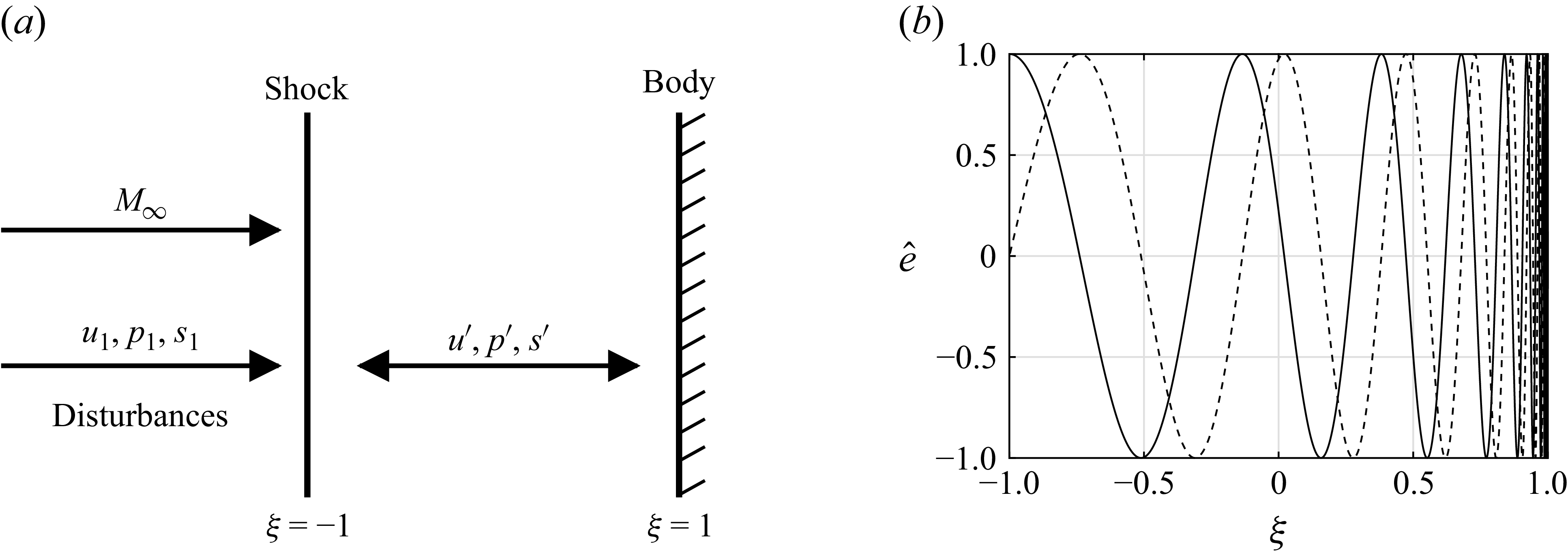
. Therefore, a numerical solution is not straightforward. Nevertheless, a scheme dealing with the singularity is devised as detailed below to solve the equations accurately. First, the acoustic (isentropic) field is solved. Then, the entropic component is found by using an analytical expression for the singularity, which allows solving only for the entropy integration constant. A sketch of the problem, adapted from Morkovin (Reference Morkovin1960), is shown in figure 1(a).
$\partial /\partial \xi$
. Therefore, a numerical solution is not straightforward. Nevertheless, a scheme dealing with the singularity is devised as detailed below to solve the equations accurately. First, the acoustic (isentropic) field is solved. Then, the entropic component is found by using an analytical expression for the singularity, which allows solving only for the entropy integration constant. A sketch of the problem, adapted from Morkovin (Reference Morkovin1960), is shown in figure 1(a).
(a) Sketch of the problem (adapted from Morkovin Reference Morkovin1960). (b) Schematic of the entropy wave $\hat {e}(\xi )$
, solid/dashed lines indicate the real/imaginary parts, respectively.
$\hat {e}(\xi )$
, solid/dashed lines indicate the real/imaginary parts, respectively.

2.4. Entropy disturbance
The entropy disturbances are found employing the following normal-mode ansatz
 \begin{equation} s'(\xi , \tau ) = \hat {s}(\xi ) e^{-i\omega \tau } + \text{c.c.}, \end{equation}
where $\hat {s}(\xi )$
represents the complex amplitude of the disturbance,
$\hat {s}(\xi )$
represents the complex amplitude of the disturbance, $\omega$
is the frequency and ‘c.c.’ denotes the complex conjugate. The linearised entropy equation is
$\omega$
is the frequency and ‘c.c.’ denotes the complex conjugate. The linearised entropy equation is
 \begin{equation} - i \omega \hat {s} + U\varXi _x\frac {{\text{d}}\hat {s}}{{\text{d}}\xi } = 0. \end{equation}
The solution to this first-order linear differential equation is given by
 \begin{equation} \hat {s}(\xi ) = \hat {s}_2 \hat {e}(\xi ),\quad \hat {e}(\xi )=\exp \int _{-1}^{\xi } \frac {i \omega }{\varXi _x U(\xi ')} \, {\text{d}}\xi ', \end{equation}
where $\hat {s}_2$
is an integration constant determined by the linearised Rankine–Hugoniot shock jump conditions at
$\hat {s}_2$
is an integration constant determined by the linearised Rankine–Hugoniot shock jump conditions at $\xi =-1$
, and
$\xi =-1$
, and $\hat {e}(\xi )$
is the normalised entropy mode shape, such that
$\hat {e}(\xi )$
is the normalised entropy mode shape, such that $\hat {e}(-1)=1$
. Since the function is singular on the body (
$\hat {e}(-1)=1$
. Since the function is singular on the body ( $\xi =1$
), it is useful to rewrite it as
$\xi =1$
), it is useful to rewrite it as
 \begin{equation} \hat {e}(\xi ) = \left (\frac {1-\xi }{2}\right )^n \exp \int _{-1}^{\xi } g(\xi ') \, {\text{d}}\xi ', \quad g(\xi )=\frac {n}{1-\xi }+\frac { i \omega }{\varXi _x U(\xi )}, \end{equation}
where $n$
is chosen such that the integrand
$n$
is chosen such that the integrand $g(\xi )$
becomes non-singular, and the integrand value on the body is found using L’Hôpital’s rule
$g(\xi )$
becomes non-singular, and the integrand value on the body is found using L’Hôpital’s rule
 \begin{equation} n = \frac {i\omega }{\varXi _x \frac {{\text{d}} U}{{\text{d}}\xi }\Big |_{\xi =1}},\quad \lim _{\xi \to 1}g(\xi )=-\frac {i\omega }{2\varXi _x}\frac {\frac {{\text{d}}^2U}{{\text{d}}\xi ^2}\Big |_{\xi =1}}{\left (\frac {{\text{d}} U}{{\text{d}}\xi }\Big |_{\xi =1}\right )^2}. \end{equation}
Near the stagnation point $\hat {e}\sim (1-\xi )^n$
, which attains values on the unit circle. The characteristic wavenumber of the oscillations,
$\hat {e}\sim (1-\xi )^n$
, which attains values on the unit circle. The characteristic wavenumber of the oscillations, $\alpha \sim \omega / U$
, tends to infinity as
$\alpha \sim \omega / U$
, tends to infinity as $U\to 0$
.
$U\to 0$
.
A sample solution of the entropy equation is shown in figure 1(b). It can be seen that the wavenumber indeed increases towards the body (and the wavelength tends to zero). The only way to circumvent the singularity is by choosing $\hat {s}_2 = 0$
, which means that there is no generation of entropy disturbances by the shock; however, this is non-physical since the shock generates entropy disturbances. Note that inclusion of even a very small amount of viscosity is expected to regularise the singularity, since eventually the disturbance wavelength becomes small enough to be comparable to the viscous length scale.
$\hat {s}_2 = 0$
, which means that there is no generation of entropy disturbances by the shock; however, this is non-physical since the shock generates entropy disturbances. Note that inclusion of even a very small amount of viscosity is expected to regularise the singularity, since eventually the disturbance wavelength becomes small enough to be comparable to the viscous length scale.
2.5. Acoustic disturbance
Similarly to the entropy, a normal-mode ansatz is used
 \begin{equation} \boldsymbol{q}' = \tilde {\boldsymbol{q}}(\xi ) e^{-i\omega \tau } + \text{c.c.}, \end{equation}
where $\omega$
is the frequency. Since, for the entropy, we only need to determine the jump across the shock
$\omega$
is the frequency. Since, for the entropy, we only need to determine the jump across the shock $\hat {s}_2$
, we define
$\hat {s}_2$
, we define
 \begin{equation} \tilde {\boldsymbol{q}} = (\hat {u}, \hat {p}, \hat {s}, \hat {x}_{s})^{\mathrm{T}} = \hat {\boldsymbol{q}} \odot (1,\, 1,\, \hat {e},\, 1)^{\mathrm{T}}, \quad \hat {\boldsymbol{q}} = (\hat {u}, \hat {p}, \hat {s}_2, \hat {x}_{s})^{\mathrm{T}}, \end{equation}
which has two unknown functions, the velocity $\hat {u}(\xi )$
and pressure
$\hat {u}(\xi )$
and pressure $\hat {p}(\xi )$
, as well as two unknown scalars, the entropy jump
$\hat {p}(\xi )$
, as well as two unknown scalars, the entropy jump $\hat {s}_2$
and the shock displacement
$\hat {s}_2$
and the shock displacement $\hat {x}_{\!s}$
. In addition, discretisation implies
$\hat {x}_{\!s}$
. In addition, discretisation implies ${\text{d}}/{\text{d}}\xi =\mathcal{D}_\xi$
. The resulting equations are
${\text{d}}/{\text{d}}\xi =\mathcal{D}_\xi$
. The resulting equations are
 \begin{align} \left (\!-i\omega + \varXi _x \frac {{\text{d}} U}{{\text{d}}\xi }+ U \varXi _x \mathcal{D}_\xi \right ) \hat {u} + \left (\frac {\varXi _x}{R} \mathcal{D}_\xi - \frac {\varXi _x}{\gamma P R}\frac {{\text{d}} P}{{\text{d}}\xi } \right ) \hat {p} + \left (\frac {\varXi _x}{\gamma R} \frac {{\text{d}} P}{{\text{d}}\xi } \hat {e} \right )\hat {s}_2 + \left (-i\omega \varXi _t \frac {{\text{d}} U}{{\text{d}}\xi } \right ) \hat {x}_{\!s} =0, \end{align}
 \begin{align} \varXi _x\! \left (\frac {{\text{d}} P}{{\text{d}}\xi } +\gamma P \mathcal{D}_\xi \right ) \hat {u}+ \left (\!-i\omega + U\varXi _x\left (\mathcal{D}_\xi -\frac {1}{P}\frac {{\text{d}} P}{{\text{d}}\xi }\right )\right ) \hat {p} + \left (\frac {\varXi _x^2}{2} \left (U\frac {{\text{d}} P}{{\text{d}}\xi } + \gamma P \frac {{\text{d}} U}{{\text{d}}\xi }\right ) - i\omega \varXi _t \frac {{\text{d}} P}{{\text{d}}\xi }\right )\hat {x}_{\!s} = 0. \end{align}
A special case arises when the base flow pressure gradient vanishes, i.e. ${\text{d}} P/{\text{d}}\xi = 0$
. In this case, the equations governing the acoustic field become decoupled from the entropy disturbance, indicating that the post-shock acoustic (isentropic) and entropy (non-isentropic) modes evolve independently. This implies that the base flow pressure gradient acts as a coupling mechanism, scattering entropy disturbances into acoustic waves and vice versa.
${\text{d}} P/{\text{d}}\xi = 0$
. In this case, the equations governing the acoustic field become decoupled from the entropy disturbance, indicating that the post-shock acoustic (isentropic) and entropy (non-isentropic) modes evolve independently. This implies that the base flow pressure gradient acts as a coupling mechanism, scattering entropy disturbances into acoustic waves and vice versa.
2.6. Combined solution
The disturbance flow field is therefore written as a sum of two solutions
 \begin{equation} \hat {\boldsymbol{q}} = \hat {\boldsymbol{q}}_i + \hat {\boldsymbol{q}}_{ii}, \end{equation}
where the acoustic (isentropic) component, $\hat {\boldsymbol{q}}_i=(\hat {u}_i, \hat {p}_i, 0, \hat {x}_{s,i})^{\text{T}}$
, is obtained by enforcing
$\hat {\boldsymbol{q}}_i=(\hat {u}_i, \hat {p}_i, 0, \hat {x}_{s,i})^{\text{T}}$
, is obtained by enforcing $\hat s_{2,i}=0$
, and the entropic component,
$\hat s_{2,i}=0$
, and the entropic component, $\hat {\boldsymbol{q}}_{ii}=(\hat {u}_{ii}, \hat {p}_{ii}, \hat {s}_2, \hat {x}_{s,ii})^{\text{T}}$
, satisfies
$\hat {\boldsymbol{q}}_{ii}=(\hat {u}_{ii}, \hat {p}_{ii}, \hat {s}_2, \hat {x}_{s,ii})^{\text{T}}$
, satisfies $\hat s_{2,ii}=\hat s_2$
. In the special case
$\hat s_{2,ii}=\hat s_2$
. In the special case ${\text{d}} P/{\text{d}}\xi =0$
, it follows that
${\text{d}} P/{\text{d}}\xi =0$
, it follows that $\hat u_{ii}=\hat p_{ii}=\hat x_{s,ii}=0$
, which means that the shock response is entirely driven by the acoustic mode, and the entropy perturbation is generated consequentially by the shock motion.
$\hat u_{ii}=\hat p_{ii}=\hat x_{s,ii}=0$
, which means that the shock response is entirely driven by the acoustic mode, and the entropy perturbation is generated consequentially by the shock motion.
2.7. Boundary conditions
The boundary conditions at the shock, derived from the linearised Rankine–Hugoniot relations, can be expressed in the following compact form. Upon applying the modal decomposition given in (2.16), these conditions become
 \begin{equation} \begin{Bmatrix} \hat {u}_2 \\[2pt] \hat {p}_2 \\[2pt] \hat {s}_2 \end{Bmatrix} = \boldsymbol{\varLambda } \begin{Bmatrix} \hat {u}_1 \\[2pt] \hat {p}_1 \\[2pt] \hat {s}_1 \end{Bmatrix} + i\omega \boldsymbol{\varPi } \hat {x}_{\!s}. \end{equation}
Here, the subscript 2 refers to the state on the high pressure side of the shock, $\xi = -1$
, while the subscript 1 denotes the incoming free-stream disturbance on the low pressure side of the shock. The coefficient values for
$\xi = -1$
, while the subscript 1 denotes the incoming free-stream disturbance on the low pressure side of the shock. The coefficient values for $\boldsymbol{\varLambda }$
and
$\boldsymbol{\varLambda }$
and $\boldsymbol{\varPi }$
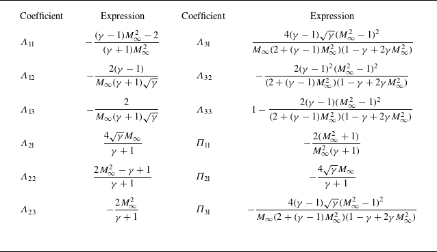
are provided in Appendix B. In our analysis, following the approach of Morkovin (Reference Morkovin1960), we consider only planar waves but examine the response to all three fundamental free-stream wave types
$\boldsymbol{\varPi }$
are provided in Appendix B. In our analysis, following the approach of Morkovin (Reference Morkovin1960), we consider only planar waves but examine the response to all three fundamental free-stream wave types
 \begin{equation} \omega _{\!e}=\alpha \sqrt {\gamma } M_\infty ,\quad \quad \omega _{\!f}=\alpha \sqrt {\gamma } \left (M_\infty +1\right )\!,\quad \omega _{\!s}=\alpha \sqrt {\gamma } \left (M_\infty -1\right )\!, \end{equation}
 \begin{equation} \begin{Bmatrix} \hat {u}_1 \\[2pt] \hat {p}_1 \\[2pt] \hat {s}_1 \end{Bmatrix}_{\!e} = \begin{Bmatrix} 0 \\[2pt] 0 \\[2pt] -\gamma \end{Bmatrix}\! , \quad \quad \begin{Bmatrix} \hat {u}_1 \\[2pt] \hat {p}_1 \\[2pt] \hat {s}_1 \end{Bmatrix}_{\!f} = \begin{Bmatrix} 1/\sqrt {\gamma } \\[3pt] 1 \\[2pt] 0 \end{Bmatrix}\! , \quad \quad \begin{Bmatrix} \hat {u}_1 \\[2pt] \hat {p}_1 \\[2pt] \hat {s}_1 \end{Bmatrix}_{\!s} = \begin{Bmatrix} -1/\sqrt {\gamma } \\[2pt] 1 \\[2pt] 0 \end{Bmatrix}\!, \end{equation}
 \begin{equation} \hat {\rho }_{1,e}=1,\quad \quad \quad \quad \quad \quad \hat {\rho }_{1,f}=1/{\gamma },\quad \quad \quad \quad \quad \hat {\rho }_{1,s}=1/{\gamma }.\quad \quad \quad \end{equation}
Here, the subscripts $e$
,
$e$
, $f$
and
$f$
and $s$
denote entropy, fast acoustic and slow acoustic waves, respectively. The parameter
$s$
denote entropy, fast acoustic and slow acoustic waves, respectively. The parameter $\alpha$
denotes the streamwise wavenumber and
$\alpha$
denotes the streamwise wavenumber and $\omega$
is the frequency. The density,
$\omega$
is the frequency. The density, $\hat {\rho }_1$
, is obtained from the linearised entropy equation,
$\hat {\rho }_1$
, is obtained from the linearised entropy equation, $\hat {s}_1 = \hat {p}_1 - \gamma \hat {\rho }_1$
. Any single-frequency planar disturbance wave can be expressed as a superposition of the three fundamental solutions above. The boundary conditions, following the decomposition in (2.19), are expressed in the following form:
$\hat {s}_1 = \hat {p}_1 - \gamma \hat {\rho }_1$
. Any single-frequency planar disturbance wave can be expressed as a superposition of the three fundamental solutions above. The boundary conditions, following the decomposition in (2.19), are expressed in the following form:
 \begin{equation} \begin{Bmatrix} \hat {u}_{2,i} \\[3pt] \hat {p}_{2,i} \\[3pt] \hat {s}_{2,i} \end{Bmatrix} = \begin{bmatrix} \boldsymbol{\varLambda }_{1\boldsymbol{\cdot }} \\[3pt] \boldsymbol{\varLambda }_{2\boldsymbol{\cdot }} \\[3pt] \boldsymbol{0} \end{bmatrix} \begin{Bmatrix} \hat {u}_1 \\[3pt] \hat {p}_1 \\[3pt] \hat {s}_1 \end{Bmatrix} + i\omega \begin{Bmatrix} \varPi _{11} \\[3pt] \varPi _{21} \\[3pt] 0 \end{Bmatrix} \hat {x}_{s,i},\quad \begin{Bmatrix} \hat {u}_{2,ii} \\[3pt] \hat {p}_{2,ii} \\[3pt] \hat {s}_{2,ii} \end{Bmatrix} = \begin{bmatrix} \boldsymbol{0} \\[3pt] \boldsymbol{0} \\[3pt] \boldsymbol{\varLambda }_{3\boldsymbol{\cdot }} \end{bmatrix} \begin{Bmatrix} \hat {u}_1 \\[3pt] \hat {p}_1 \\[3pt] \hat {s}_1 \end{Bmatrix} + i\omega \begin{Bmatrix} 0 \\[3pt] 0 \\[3pt] \varPi _{31} \end{Bmatrix} \hat {x}_{s,i} + i\omega \boldsymbol{\varPi } \hat {x}_{s,ii}. \end{equation}
The remaining boundary condition is the no-penetration condition on the body
 \begin{equation} \hat {u}(\xi =1) = \hat {u}_i(\xi =1)= \hat {u}_{ii}(\xi =1) = 0. \end{equation}
The linearised equations were solved on a Chebyshev grid, with 250 collocation points.
3. Results
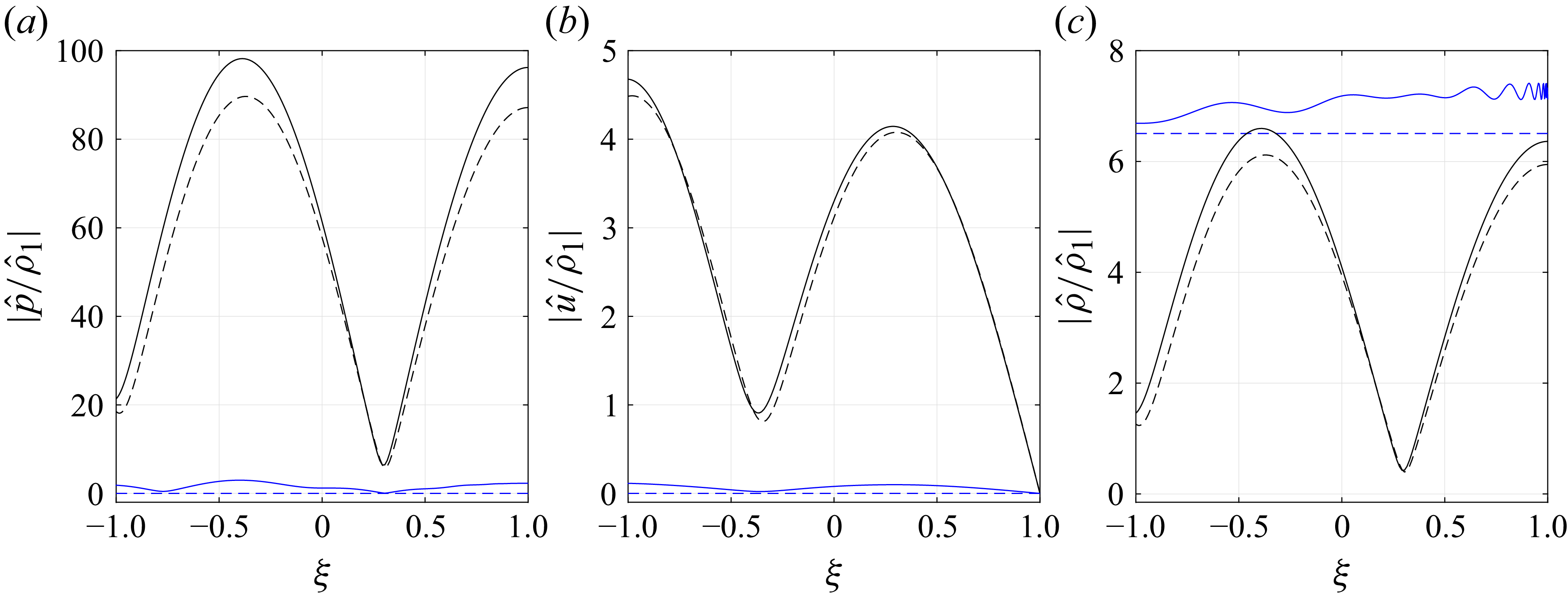
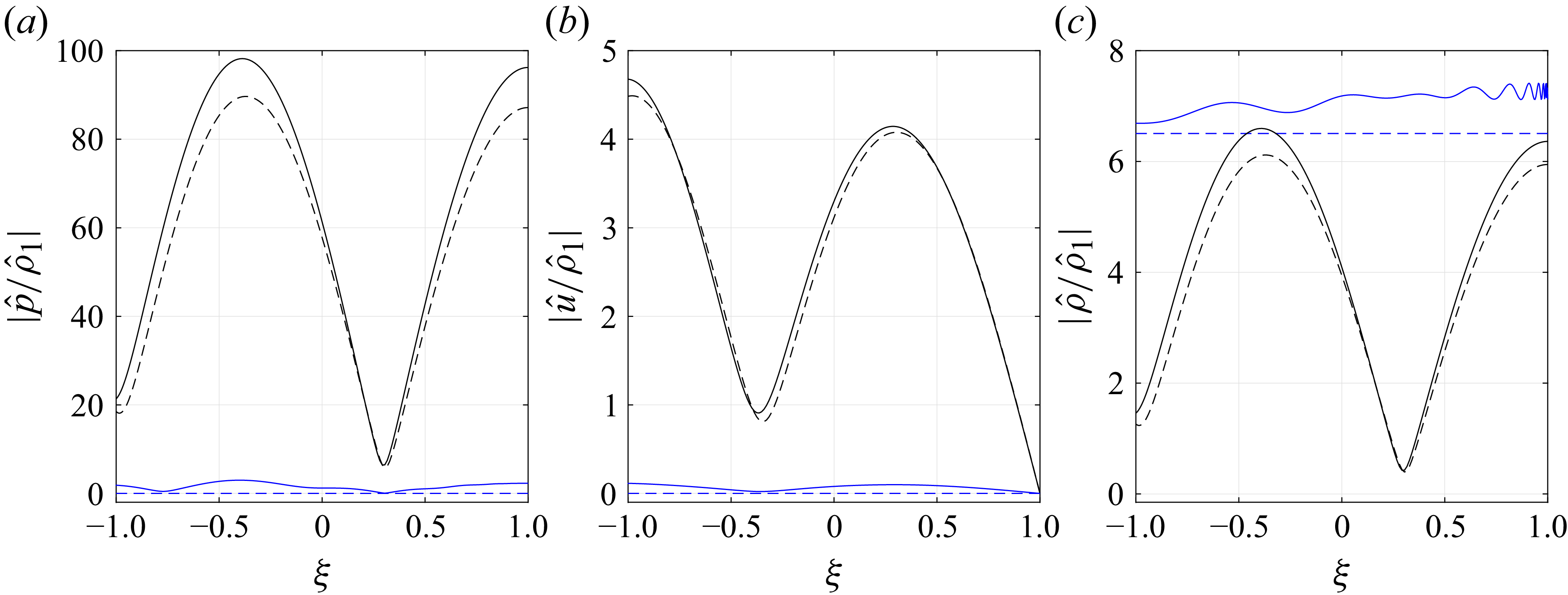
A cylinder at $M_\infty = 7$
is chosen as a representative case. Initially, the response of the flow on the stagnation line to an incoming entropy wave with frequency
$M_\infty = 7$
is chosen as a representative case. Initially, the response of the flow on the stagnation line to an incoming entropy wave with frequency $\omega = 40$
is examined. Then, a frequency sweep is conducted, followed by a variation of the Mach number. The amplitudes of
$\omega = 40$
is examined. Then, a frequency sweep is conducted, followed by a variation of the Mach number. The amplitudes of $\hat {p}$
,
$\hat {p}$
, $\hat {u}$
and
$\hat {u}$
and $\hat {\rho }$
for the acoustic (
$\hat {\rho }$
for the acoustic ( $\hat {\boldsymbol{q}}_i$
) and entropic (
$\hat {\boldsymbol{q}}_i$
) and entropic ( $\hat {\boldsymbol{q}}_{ii}$
) components are shown by the solid black and blue lines in figure 2, respectively, with the density perturbation,
$\hat {\boldsymbol{q}}_{ii}$
) components are shown by the solid black and blue lines in figure 2, respectively, with the density perturbation, $\hat {\rho }$
, obtained from
$\hat {\rho }$
, obtained from $\hat {s} = \hat {p}/P - \gamma \hat {\rho }/R$
. Although the total density perturbation includes comparable acoustic and entropic contributions, the pressure and velocity disturbances are dominated by the acoustic (isentropic) mode, for which
$\hat {s} = \hat {p}/P - \gamma \hat {\rho }/R$
. Although the total density perturbation includes comparable acoustic and entropic contributions, the pressure and velocity disturbances are dominated by the acoustic (isentropic) mode, for which $\hat {\rho } = (R / \gamma P)\hat {p}$
. Therefore, it is justified to disregard the entropic component when the velocity and pressure fields are of primary interest.
$\hat {\rho } = (R / \gamma P)\hat {p}$
. Therefore, it is justified to disregard the entropic component when the velocity and pressure fields are of primary interest.
The base flow pressure gradient, ${\text{d}} P/{\text{d}}\xi$
, introduces a coupling between the acoustic and entropic modes, which is quantified by comparison with the solution assuming
${\text{d}} P/{\text{d}}\xi$
, introduces a coupling between the acoustic and entropic modes, which is quantified by comparison with the solution assuming ${\text{d}} P/{\text{d}}\xi =0$
, indicated by the dashed lines. The solution neglecting
${\text{d}} P/{\text{d}}\xi =0$
, indicated by the dashed lines. The solution neglecting ${\text{d}} P/{\text{d}}\xi$
assumes uniform pressure and density while retaining the actual velocity distribution. Only minor quantitative changes in the solution are observed. Therefore, omitting the term
${\text{d}} P/{\text{d}}\xi$
assumes uniform pressure and density while retaining the actual velocity distribution. Only minor quantitative changes in the solution are observed. Therefore, omitting the term ${\text{d}} P/{\text{d}}\xi$
provides a justified simplification that preserves the essential characteristics of the flow while reducing the analytical complexity. The shock displacement amplitudes are
${\text{d}} P/{\text{d}}\xi$
provides a justified simplification that preserves the essential characteristics of the flow while reducing the analytical complexity. The shock displacement amplitudes are $|\hat {x}_{s,i}/\hat {\rho }_1| = 0.142$
and
$|\hat {x}_{s,i}/\hat {\rho }_1| = 0.142$
and $|\hat {x}_{s,ii}/\hat {\rho }_1| = 0.003$
, indicating that the acoustic component dominates the shock response. In the absence of the base flow pressure gradient, only the acoustic response remains, with
$|\hat {x}_{s,ii}/\hat {\rho }_1| = 0.003$
, indicating that the acoustic component dominates the shock response. In the absence of the base flow pressure gradient, only the acoustic response remains, with $|\hat {x}_{\!s}/\hat {\rho }_1|=|\hat {x}_{s,i}/\hat {\rho }_1| = 0.136$
.
$|\hat {x}_{\!s}/\hat {\rho }_1|=|\hat {x}_{s,i}/\hat {\rho }_1| = 0.136$
.
Acoustic $\square _i$
(black) and entropic
$\square _i$
(black) and entropic $\square _{ii}$
(
$\square _{ii}$
( ) components with (solid) and without (dashed) the base flow pressure gradient, for a cylinder at $M_\infty = 7$
and free-stream entropy wave with
$M_\infty = 7$
and free-stream entropy wave with $\omega = 40$
(
$\omega = 40$
( $\tilde \omega = 2.9$
). (a) Pressure. (b) Velocity. (c) Density.
$\tilde \omega = 2.9$
). (a) Pressure. (b) Velocity. (c) Density.
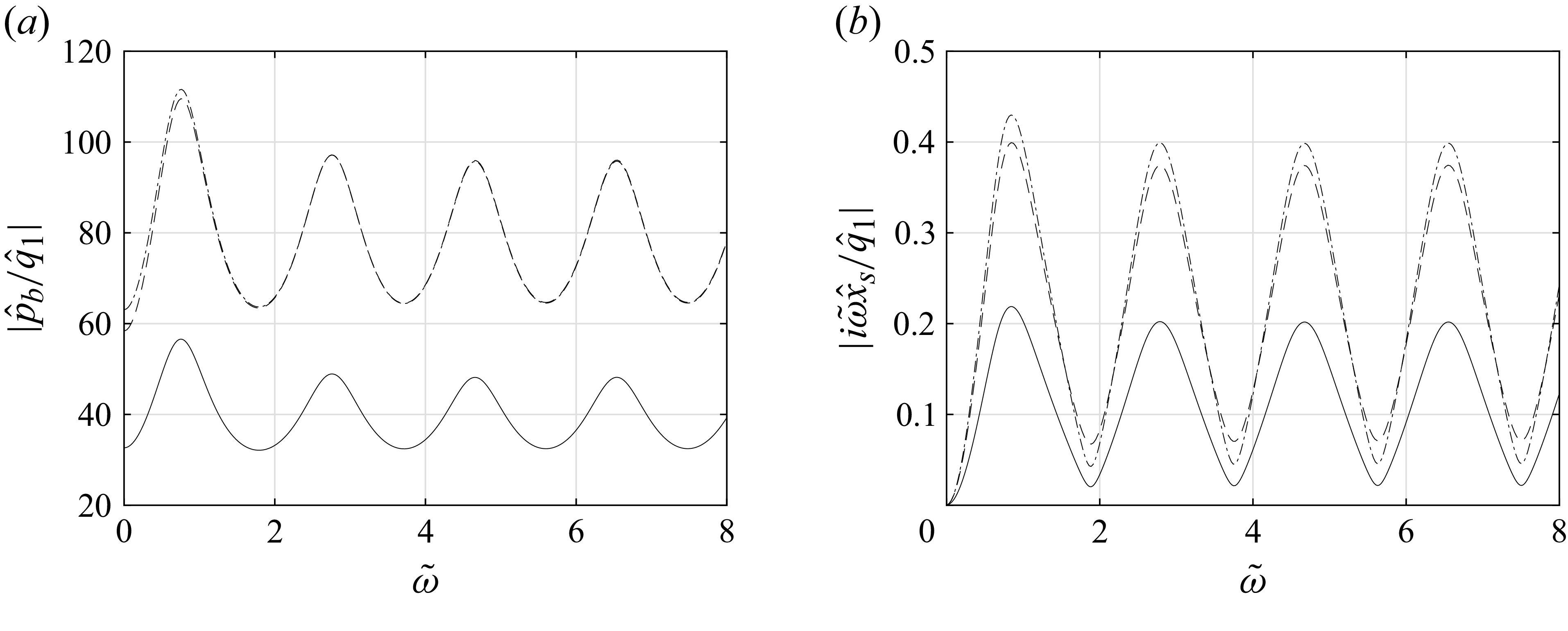
(a) Disturbance pressure amplitude on the body, $|\hat {p}_b|$
, and (b) shock velocity amplitude,
$|\hat {p}_b|$
, and (b) shock velocity amplitude, $|i\tilde {\omega }\hat {x}_{\!s}|$
, vs. rescaled frequency
$|i\tilde {\omega }\hat {x}_{\!s}|$
, vs. rescaled frequency $\tilde {\omega }$
, for incoming slow acoustic (solid); entropy (dashed–dotted); and fast acoustic (dashed) waves, for a cylinder at
$\tilde {\omega }$
, for incoming slow acoustic (solid); entropy (dashed–dotted); and fast acoustic (dashed) waves, for a cylinder at $M_\infty = 7$
.
$M_\infty = 7$
.
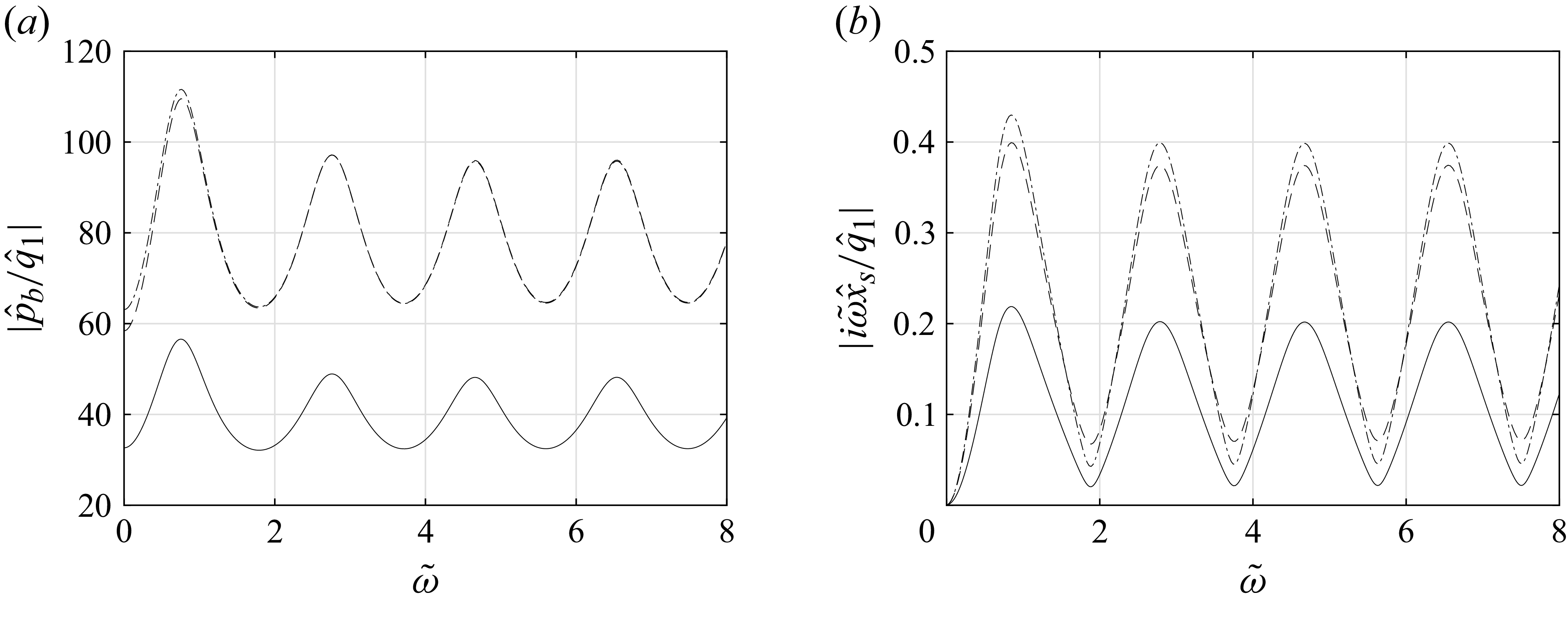
The frequency shown in figure 2 corresponds to the second peak that maximises the disturbance pressure on the body (see figure 3 and related discussion in the next subsection). For this frequency, there is a constructive interference between the fast and slow acoustic waves, that can be quantified by the ratio between the values of the acoustic pressure and density on the body and the shock, yielding $\hat {p}_{b,i}/\hat {p}_{2,i} \approx \hat {\rho }_{b,i}/\hat {\rho }_{2,i} \approx 4.5$
. The entropic density component, however, grows only slightly from the shock to the body due to the rise in base flow density, and the oscillatory behaviour of the entropy wave (figure 1
b) is visible as
$\hat {p}_{b,i}/\hat {p}_{2,i} \approx \hat {\rho }_{b,i}/\hat {\rho }_{2,i} \approx 4.5$
. The entropic density component, however, grows only slightly from the shock to the body due to the rise in base flow density, and the oscillatory behaviour of the entropy wave (figure 1
b) is visible as $\xi \to 1$
. Since the velocity perturbations of the acoustic waves are of opposite phases, the acoustic velocity disturbance attains local minima where the acoustic pressure attains local maxima and vice versa. For the frequency of the first peak that maximises the disturbance pressure on the body, monotonic increase (decrease) of the acoustic pressure (velocity) is observed, with the extrema attained at the boundaries (not shown here).
$\xi \to 1$
. Since the velocity perturbations of the acoustic waves are of opposite phases, the acoustic velocity disturbance attains local minima where the acoustic pressure attains local maxima and vice versa. For the frequency of the first peak that maximises the disturbance pressure on the body, monotonic increase (decrease) of the acoustic pressure (velocity) is observed, with the extrema attained at the boundaries (not shown here).
3.1. Effect of frequency
The effect of frequency is assessed by examining the pressure disturbance amplitude on the body, $|\hat {p}_b|$
, and the shock velocity amplitude,
$|\hat {p}_b|$
, and the shock velocity amplitude, $|i\tilde {\omega }\hat {x}_{\!s}|$
, shown in figures 3(a) and 3(b), respectively. The values are normalised by the free-stream disturbance amplitude
$|i\tilde {\omega }\hat {x}_{\!s}|$
, shown in figures 3(a) and 3(b), respectively. The values are normalised by the free-stream disturbance amplitude $|\hat {q}_1|$
, which for the acoustic modes is
$|\hat {q}_1|$
, which for the acoustic modes is $\hat {q}_1 = \hat {p}_1$
, while for the entropy mode it is
$\hat {q}_1 = \hat {p}_1$
, while for the entropy mode it is $\hat {q}_1 = \hat {\rho }_1$
. The frequency is rescaled as follows:
$\hat {q}_1 = \hat {\rho }_1$
. The frequency is rescaled as follows:
 \begin{equation} \tilde {\omega } = \frac {2 \omega \Delta }{\pi \sqrt {\gamma P_0 / R_0}}, \end{equation}
where $\varDelta$
is the shock standoff distance,
$\varDelta$
is the shock standoff distance, $P_0$
is the stagnation pressure and
$P_0$
is the stagnation pressure and $R_0$
is the stagnation density. This renormalisation, as obtained from the analytical solution presented in Morkovin (Reference Morkovin1960), places the extrema of the disturbance pressure on the body at integer values of
$R_0$
is the stagnation density. This renormalisation, as obtained from the analytical solution presented in Morkovin (Reference Morkovin1960), places the extrema of the disturbance pressure on the body at integer values of $\tilde {\omega }$
for uniform post-shock flows. In the present results for
$\tilde {\omega }$
for uniform post-shock flows. In the present results for $M_\infty = 7$
, a shift in the location of these extrema is observed compared with the prediction based on uniform flow. The first peak, which occurs at
$M_\infty = 7$
, a shift in the location of these extrema is observed compared with the prediction based on uniform flow. The first peak, which occurs at $\tilde \omega \approx 0.75$
, in both pressure and shock velocity amplitudes, is the highest, with comparable amplification of fast acoustic disturbances (dashed lines) and entropy waves (dashed–dotted lines). Slow acoustic waves (solid lines) reach approximately 50 % of the response to fast acoustic waves.
$\tilde \omega \approx 0.75$
, in both pressure and shock velocity amplitudes, is the highest, with comparable amplification of fast acoustic disturbances (dashed lines) and entropy waves (dashed–dotted lines). Slow acoustic waves (solid lines) reach approximately 50 % of the response to fast acoustic waves.
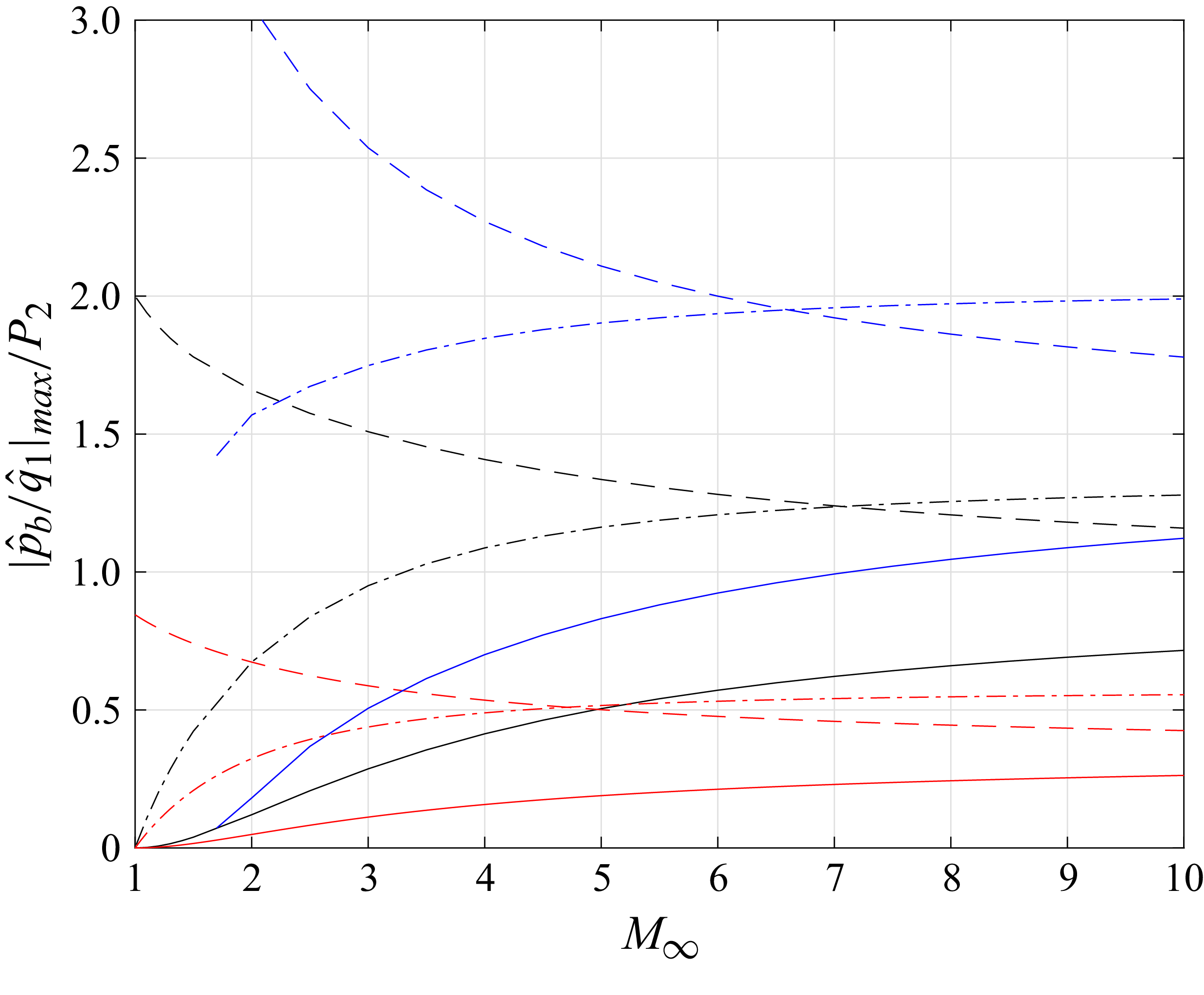
Maximum amplitude of the disturbance pressure on the body, $|\hat {p}_b|_{\textit{max}}$
, vs. Mach number. Actual flow (), uniform flow (black) and no reflections (
$|\hat {p}_b|_{\textit{max}}$
, vs. Mach number. Actual flow (), uniform flow (black) and no reflections ( ). Incoming slow acoustic (solid); entropy (dashed–dotted); and fast acoustic (dashed) waves.
3.2. Effect of Mach number
The effect of the free-stream Mach number, $M_\infty$
, is quantified by examining the maximum amplitude of the disturbance pressure on the body,
$M_\infty$
, is quantified by examining the maximum amplitude of the disturbance pressure on the body, $|\hat {p}_b|_{\textit{max}}$
, attained at
$|\hat {p}_b|_{\textit{max}}$
, attained at $\tilde \omega \approx 0.75$
. The value of
$\tilde \omega \approx 0.75$
. The value of $|\hat {p}_b/\hat {q}_1|_{\textit{max}}$
, normalised by the base flow post-shock pressure
$|\hat {p}_b/\hat {q}_1|_{\textit{max}}$
, normalised by the base flow post-shock pressure $P_2$
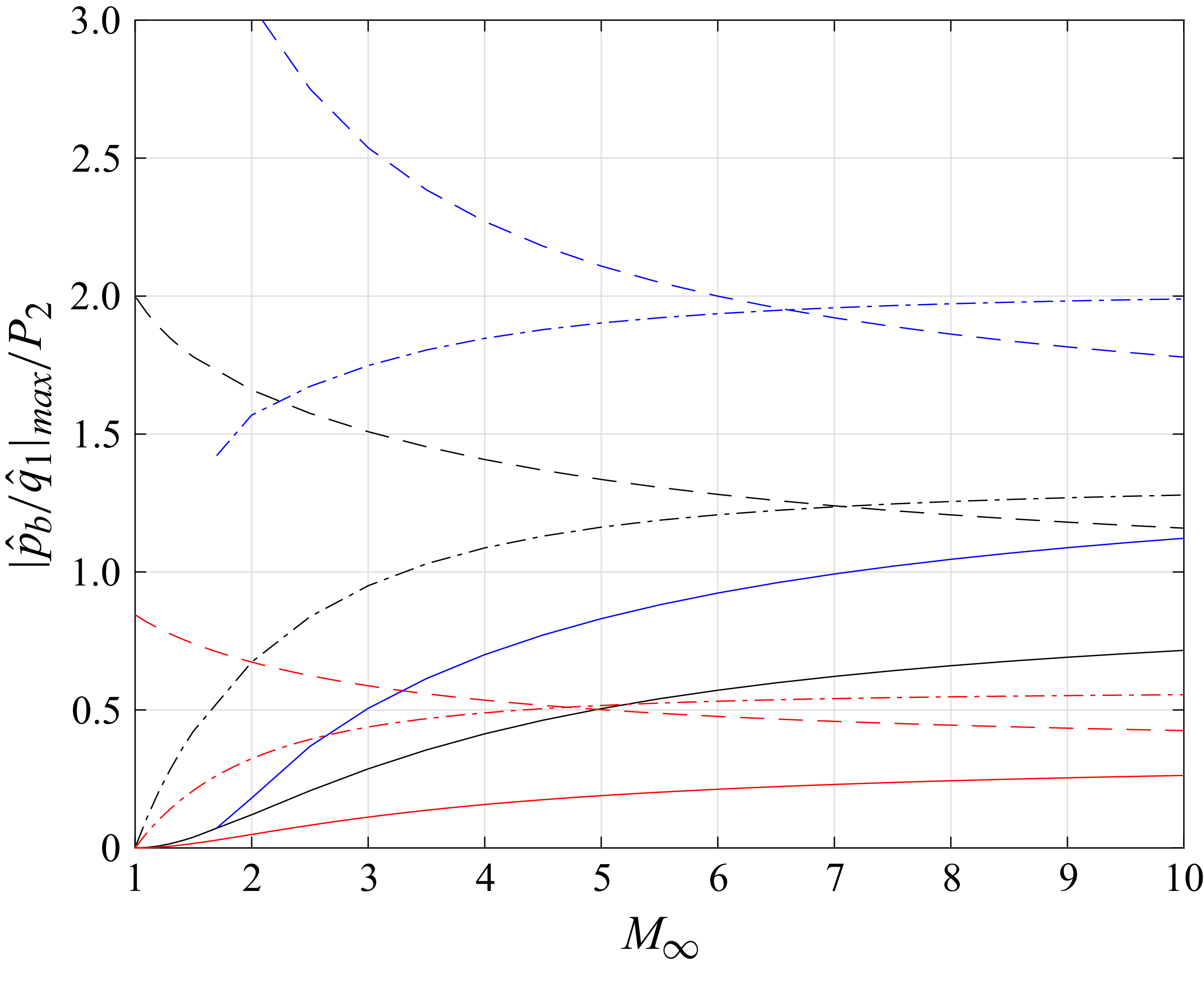
, is shown in figure 4 for the three types of free-stream disturbances: slow acoustic (solid lines), entropy (dashed–dotted lines) and fast acoustic (dashed lines). Three different configurations are compared: actual decelerating stagnation-line flows are coloured blue, the simplified uniform post-shock flow proposed by Morkovin (Reference Morkovin1960) is coloured black and the response of the shock neglecting reflections from the body as analysed by Ribner (Reference Ribner1954a
) is coloured red. The results show that, as expected, the presence of the body always leads to amplification of the incoming disturbances. The actual flow (blue) leads to approximately 50 % higher amplification compared with the uniform flow (black). Among the disturbance types, for Mach numbers smaller than approximately 6.6 the fast acoustic wave is the most highly amplified, followed by the entropy wave and finally the slow acoustic wave. For Mach numbers above approximately 6.6 the entropy wave surpasses the fast acoustic wave. The amplification trends with the Mach number vary between the slow acoustic and entropy waves, which increase with
$P_2$
, is shown in figure 4 for the three types of free-stream disturbances: slow acoustic (solid lines), entropy (dashed–dotted lines) and fast acoustic (dashed lines). Three different configurations are compared: actual decelerating stagnation-line flows are coloured blue, the simplified uniform post-shock flow proposed by Morkovin (Reference Morkovin1960) is coloured black and the response of the shock neglecting reflections from the body as analysed by Ribner (Reference Ribner1954a
) is coloured red. The results show that, as expected, the presence of the body always leads to amplification of the incoming disturbances. The actual flow (blue) leads to approximately 50 % higher amplification compared with the uniform flow (black). Among the disturbance types, for Mach numbers smaller than approximately 6.6 the fast acoustic wave is the most highly amplified, followed by the entropy wave and finally the slow acoustic wave. For Mach numbers above approximately 6.6 the entropy wave surpasses the fast acoustic wave. The amplification trends with the Mach number vary between the slow acoustic and entropy waves, which increase with $M_\infty$
, and the fast acoustic wave, which decreases with
$M_\infty$
, and the fast acoustic wave, which decreases with $M_\infty$
. All responses level off at higher Mach numbers, as
$M_\infty$
. All responses level off at higher Mach numbers, as $M_\infty \to \infty$
.
$M_\infty \to \infty$
.
4. Discussion and conclusions
The receptivity problem targeted at the flow on the stagnation line of blunt bodies in supersonic flow is formulated and solved by combining a spectral shock-fitting algorithm with a linear disturbance analysis. While reproducing the results of Morkovin (Reference Morkovin1960) for uniform post-shock flow, a wrong sign was identified in one of the coefficients, inadvertently suggesting damping by the body; with the corrected sign, the presence of the body amplifies disturbances. Our main findings are as follows:
-
(i) Acoustic disturbances dominate pressure and velocity responses, while the density response is influenced by both acoustic and entropy modes.
-
(ii) Post-shock entropy disturbances exhibit singular behaviour near the stagnation point, with their wavenumber stretching to infinity.
-
(iii) The base flow pressure gradient introduces a coupling between acoustic and entropic disturbances; however, since these are relatively minor corrections, it is justified to neglect the base flow pressure gradient.
-
(iv) The maximal disturbance pressure on the body occurs when the rescaled frequency $\tilde \omega$
is approximately 0.75.
$\tilde \omega$
is approximately 0.75. -
(v) The realistic stagnation-line base flow amplifies all disturbance types approximately 50 % higher compared with the idealised uniform post-shock flow.
-
(vi) The amplification of fast acoustic waves decreases with
$M_\infty$
, while the response to entropy and slow acoustic waves increases with
$M_\infty$
. The most amplified disturbance changes from the fast acoustic to the entropy wave at
$M_\infty \approx 6.6$
. All responses level off as the Mach number increases.


The applicability of the one-dimensional model to actual two-dimensional (planar or axisymmetric) flows is an important subject for future research. In addition, the interaction of the shock with vorticity disturbances, which does not exist in one-dimensional flow, and disturbances which are oblique with respect to the stagnation streamline, also require further investigation.
Funding
The research was supported by an internal grant from Technion Israel Institute of Technology.
Declaration of interests
The authors report no conflict of interest.
Appendix A. Discussion and correction of the analysis by Morkovin (Reference Morkovin1960)
It should be noted that all the mathematical expressions in Morkovin (Reference Morkovin1960) are correct. However, the plots and conclusions drawn from them are not, due to an inadvertently added minus sign to $\varPi _{31}$
. This coefficient
$\varPi _{31}$
. This coefficient
 \begin{equation} \varPi _{31} = \frac {1}{1 - M^2}\left (1 - \frac {\rho _{1m}}{\rho _{m}}\right ) \left (1 + M^2 + (\gamma - 1)\left (1 - \frac {\rho _{m}}{\rho _{1m}}\right ) M^2\right )\!, \end{equation}
is always positive; however, throughout Morkovin (Reference Morkovin1960) it was consistently used with a minus sign. In the above expression $M$
is the post-shock Mach number and
$M$
is the post-shock Mach number and $\rho _{m}/\rho _{1m}$
is the density ratio across the shock. Note that all the expressions in this appendix refer to their definitions in Morkovin (Reference Morkovin1960).
$\rho _{m}/\rho _{1m}$
is the density ratio across the shock. Note that all the expressions in this appendix refer to their definitions in Morkovin (Reference Morkovin1960).
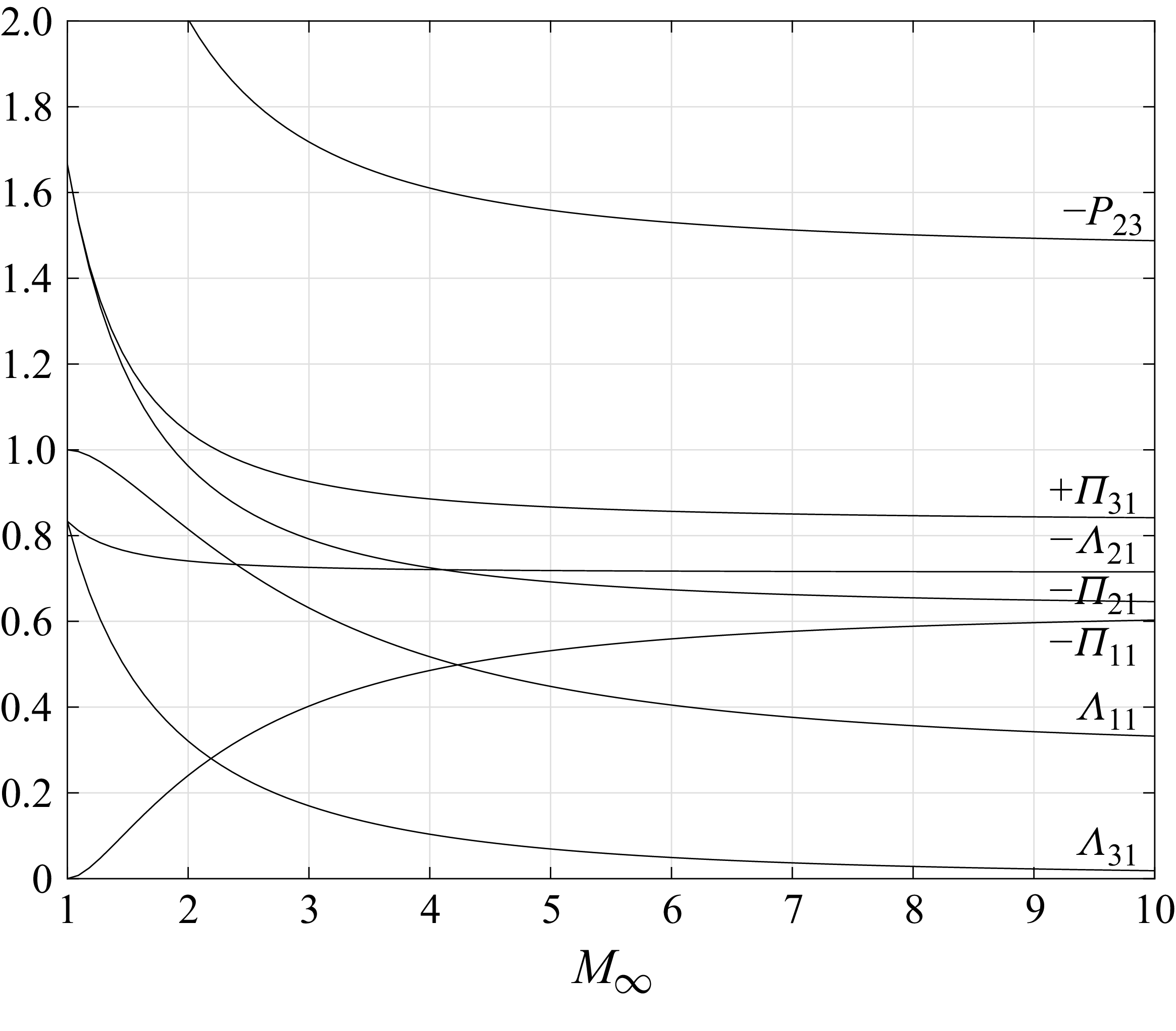
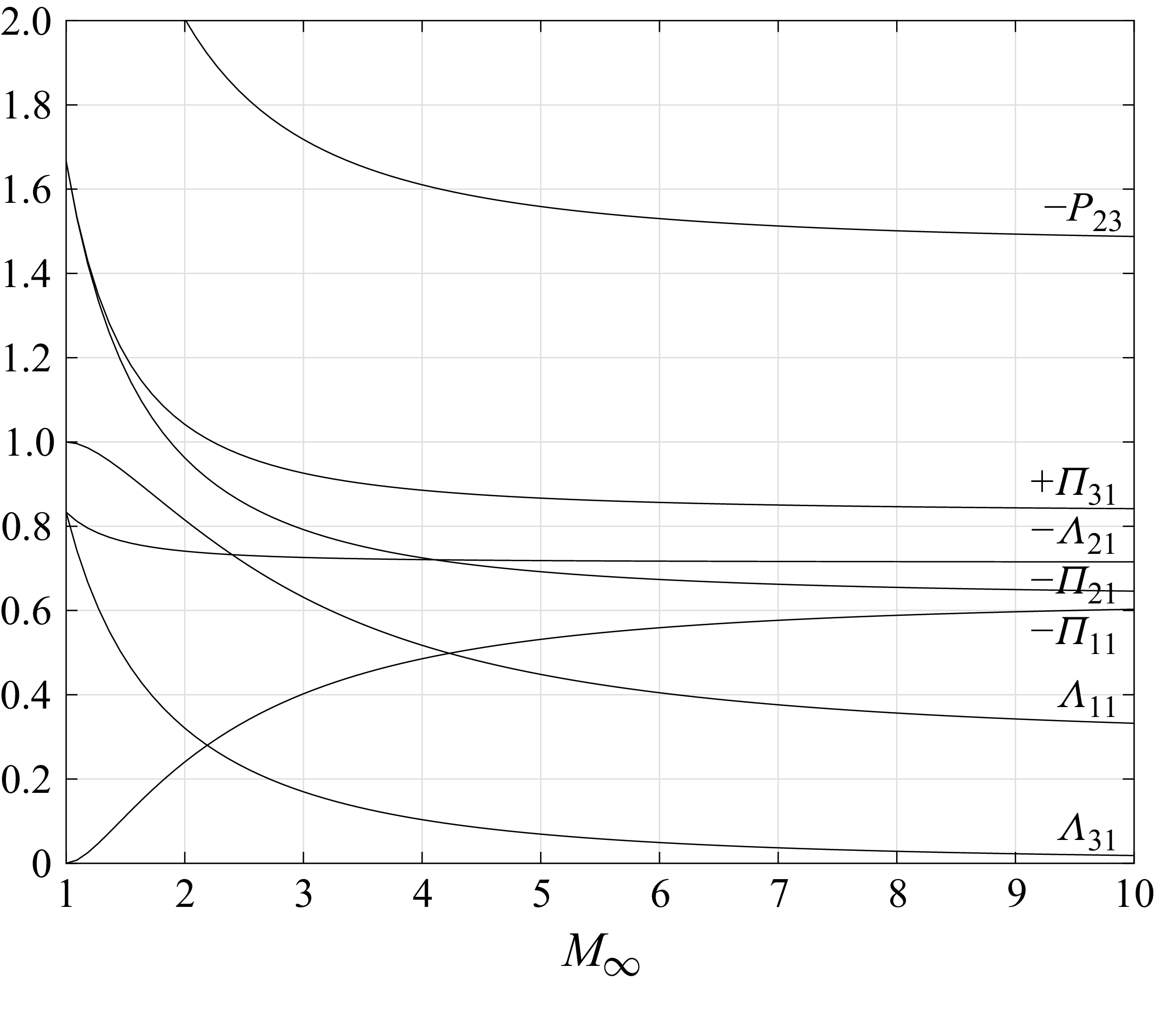
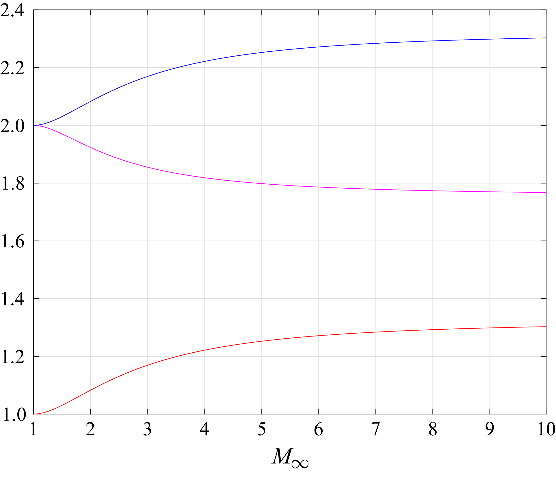
Corrected figure 2 from Morkovin (Reference Morkovin1960), with $+\varPi _{31}$
and
$+\varPi _{31}$
and $-P_{23}$
.
$-P_{23}$
.
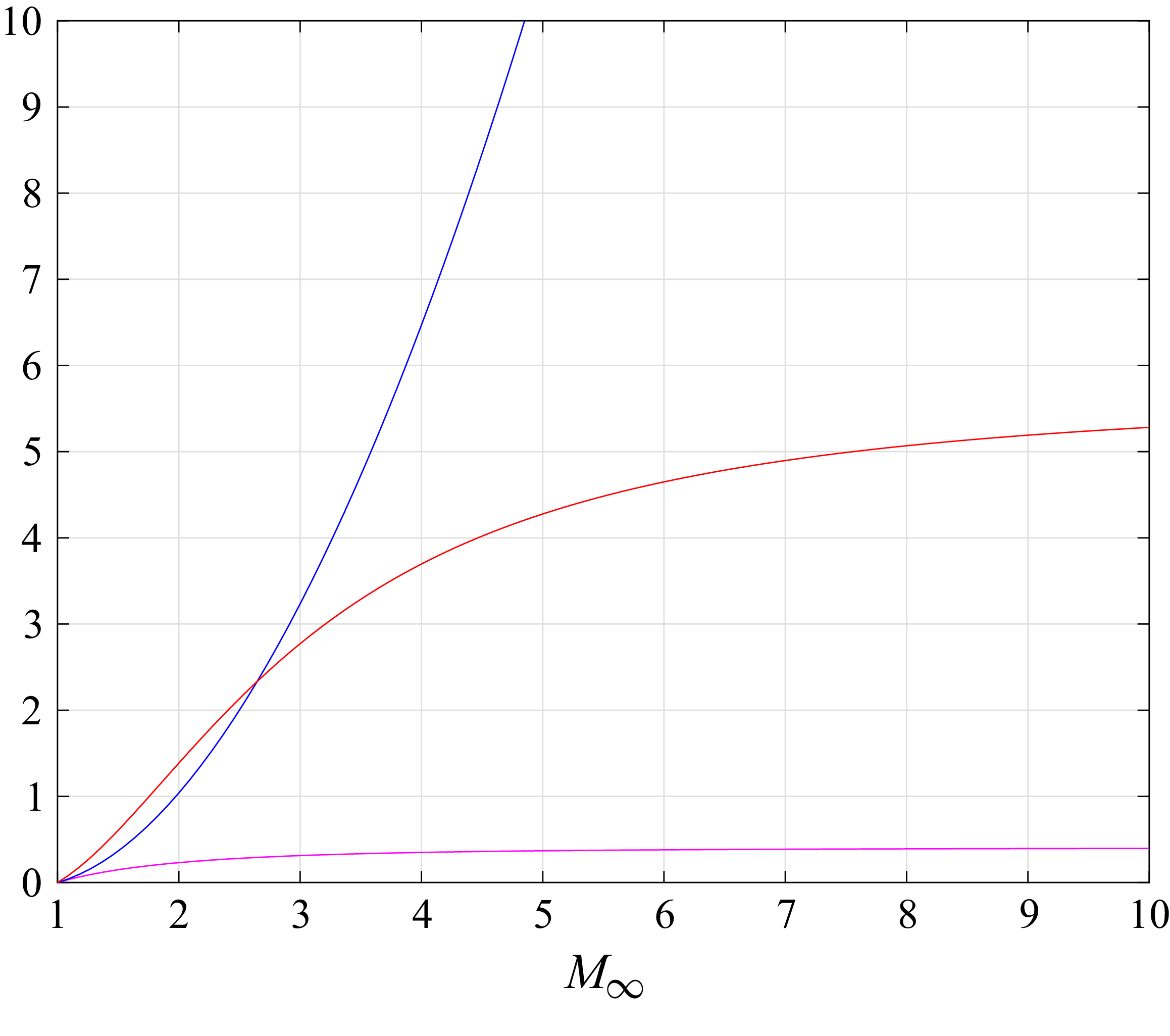
Corrected figure 3 from Morkovin (Reference Morkovin1960), (8a) (); $|({\delta p_+}/{({\gamma }/{2}) p_m M^2})/({\delta T_-}/{T_{1m}})|$
();
$|({\delta p_+}/{({\gamma }/{2}) p_m M^2})/({\delta T_-}/{T_{1m}})|$
(); $|{\varDelta _{23}}/{P_{23}}|$
(7a) (
$|{\varDelta _{23}}/{P_{23}}|$
(7a) ( ).
).

Coefficients $\varLambda _{ij}$
and
$\varLambda _{ij}$
and $\varPi _{ij}$
.
$\varPi _{ij}$
.

Corrected figure 5 from Morkovin (Reference Morkovin1960), $|{P_{23}}/{\varPi _{21}}|$
(13b) ();
$|{P_{23}}/{\varPi _{21}}|$
(13b) (); $|{P_{23}}/{\varPi _{31}}|$
(13c) (); max of (14)
$|{P_{23}}/{\varPi _{31}}|$
(13c) (); max of (14) $|{\varPi _{31}}/{\varPi _{21}}|$
().
$|{\varPi _{31}}/{\varPi _{21}}|$
().
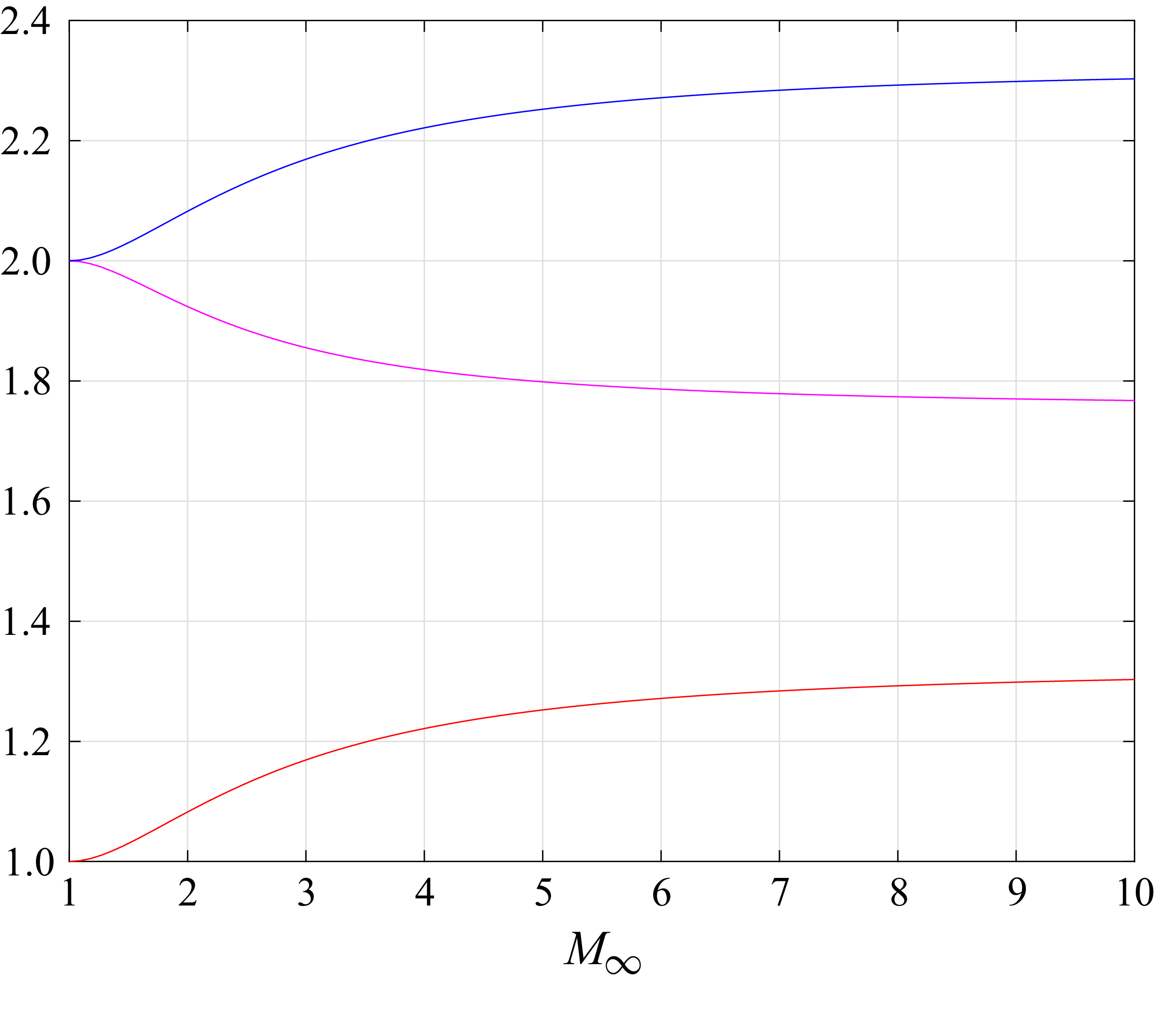
The corrected versions of figures 2, 3 and 5 in Morkovin (Reference Morkovin1960) (without the inadvertently added minus sign to $\varPi _{31}$
) are shown in figures 5, 6 and 7, respectively. In figure 5 only the curves of
$\varPi _{31}$
) are shown in figures 5, 6 and 7, respectively. In figure 5 only the curves of $\varPi _{31}$
and
$\varPi _{31}$
and $P_{23}$
are different from the original (figure 2 in Morkovin Reference Morkovin1960). Note that
$P_{23}$
are different from the original (figure 2 in Morkovin Reference Morkovin1960). Note that $P_{23}=\varPi _{21}-\varPi _{31}$
is negative, therefore, a minus sign is added to it to consistently plot only positive quantities. In figure 6 all coefficients smoothly decrease to 0 as
$P_{23}=\varPi _{21}-\varPi _{31}$
is negative, therefore, a minus sign is added to it to consistently plot only positive quantities. In figure 6 all coefficients smoothly decrease to 0 as ${M_\infty}\to 1$
, compared with the divergent behaviour in the original (figure 3 in Morkovin Reference Morkovin1960). In figure 7, the values of
${M_\infty}\to 1$
, compared with the divergent behaviour in the original (figure 3 in Morkovin Reference Morkovin1960). In figure 7, the values of $|{P_{23}}/{\varPi _{21}}|$
and
$|{P_{23}}/{\varPi _{21}}|$
and $|{P_{23}}/{\varPi _{31}}|$
, which are the multiplying factors as a result of the body, are close to 2, which implies that reflections from the body lead to amplification of disturbances, compared with values lower than unity in the original (figure 5 in Morkovin Reference Morkovin1960).
$|{P_{23}}/{\varPi _{31}}|$
, which are the multiplying factors as a result of the body, are close to 2, which implies that reflections from the body lead to amplification of disturbances, compared with values lower than unity in the original (figure 5 in Morkovin Reference Morkovin1960).














 Open access

