2 The Narimanov–Moiseev-type modal equations

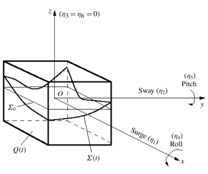
A cyclically moving rigid square base container is partially filled with a finite liquid depth by a perfect incompressible (irrotational flows) liquid. Figure 1 introduces necessary notation including the prescribed time-periodic translatory $\boldsymbol{v}_{O}(t)=(\dot{\unicode[STIX]{x1D702}}_{1}(t),\dot{\unicode[STIX]{x1D702}}_{2}(t),0)$ and instant angular $\unicode[STIX]{x1D74E}(t)=(\dot{\unicode[STIX]{x1D702}}_{4}(t),\dot{\unicode[STIX]{x1D702}}_{5}(t),\dot{\unicode[STIX]{x1D702}}_{6}(t))$ velocities of the container, which satisfy the periodicity condition $\boldsymbol{v}_{O}(t+T)=\boldsymbol{v}_{O}(t)$ and $\unicode[STIX]{x1D74E}(t+T)=\unicode[STIX]{x1D74E}(t)$, where $T=2\unicode[STIX]{x03C0}/\unicode[STIX]{x1D70E}$ is the forcing period. The developed nonlinear sloshing theory below requires that the heave container component is zero ($\unicode[STIX]{x1D702}_{3}(t)\equiv 0$) to avoid parametric resonances in the hydrodynamic system (see a recent review on the parametric waves by Ibrahim (Reference Ibrahim2015)).

Figure 1.

A rigid square base container moves cyclically with a small amplitude in surge, sway, roll, pitch and yaw so that its translatory velocity is $\boldsymbol{v}_{O}(t)=(v_{O1}(t),v_{O2}(t),0)=(\dot{\unicode[STIX]{x1D702}}_{1}(t),\dot{\unicode[STIX]{x1D702}}_{2}(t),0)$ and the instant angular velocity is $\unicode[STIX]{x1D74E}(t)=(\unicode[STIX]{x1D714}_{1}(t),\unicode[STIX]{x1D714}_{2}(t),\unicode[STIX]{x1D714}_{3}(t))=(\dot{\unicode[STIX]{x1D702}}_{4}(t),\dot{\unicode[STIX]{x1D702}}_{5}(t),\dot{\unicode[STIX]{x1D702}}_{6}(t))$. The $Oxyz$ coordinate system is rigidly fixed with the container. The mean (hydrostatic) free surface $\unicode[STIX]{x1D6F4}_{0}$ belongs to the $Oxy$ plane and the origin is in the geometric centre of $\unicode[STIX]{x1D6F4}_{0}$. In the non-dimensional statement, the tank breadth and width are equal to the unit but the non-dimensional mean liquid depth equals to $h$.

Oscillatory liquid motions (sloshing) are considered in the non-inertial (tank-fixed) coordinate system $Oxyz$ whose $Oxy$-plane coincides with the mean (hydrostatic) free surface $\unicode[STIX]{x1D6F4}_{0}$ and $Oz$ runs through the centre of $\unicode[STIX]{x1D6F4}_{0}$. Mathematically, the sloshing problem consists of finding the two unknowns: the free surface $\unicode[STIX]{x1D6F4}(t)$ (described by the single-value representation $z=f(x,y,t)$) and the absolute velocity potential $\unicode[STIX]{x1D6F7}(x,y,z,t)$. The corresponding free-surface problem and its variational analogy are presented in Part 1 (see more mathematical and physical details in chap. 2 of Faltinsen & Timokha (Reference Faltinsen and Timokha2009)).

The present paper concentrates on the steady-state waves, which are associated with the $(T=2\unicode[STIX]{x03C0}/\unicode[STIX]{x1D70E})$-periodic solutions, $f(x,y,t+T)=f(x,y,t)$ and $\unicode[STIX]{x1D735}\unicode[STIX]{x1D6F7}(x,y,z,t+T)=\unicode[STIX]{x1D735}\unicode[STIX]{x1D6F7}(x,y,z,t)$, of the sloshing problem and their stability. The periodic solutions (for longitudinal, diagonal and oblique tank reciprocations) were constructed in Parts 1 and 4 by employing an asymptotic (modal) theory by Narimanov (Reference Narimanov1957) and Moiseev (Reference Moiseev1958). The theory suggests the small (relative to the tank breadth $L$) non-dimensional tank forcing,

(2.1)$$\begin{eqnarray}\unicode[STIX]{x1D702}_{i}(t)\sim O(\unicode[STIX]{x1D716})\ll 1,\quad i=1,2,4,5,6,\end{eqnarray}$$

where $\unicode[STIX]{x1D702}_{i}(t)$ are the above-introduced five degrees of freedom of the moving tank, and the $L$-scaled modal representation of the free surface

(2.2)$$\begin{eqnarray}\displaystyle f(x,y,t) & = & \displaystyle \underbrace{a_{1}(t)f_{1}^{(1)}(x)+b_{1}(t)f_{1}^{(2)}(y)}_{O(\unicode[STIX]{x1D716}^{1/3})}+\underbrace{a_{2}(t)f_{2}^{(1)}(x)+b_{2}(t)f_{2}^{(2)}(y)+c_{1}(t)f_{1}^{(1)}(x)f_{1}^{(2)}(y)}_{O(\unicode[STIX]{x1D716}^{2/3})}\nonumber\\ \displaystyle & & \displaystyle +\,\underbrace{a_{3}(t)f_{3}^{(1)}(x)+b_{3}(t)f_{3}^{(2)}(y)+c_{21}(t)f_{2}^{(1)}(x)f_{1}^{(2)}(y)+c_{12}(t)f_{1}^{(1)}(x)f_{2}^{(2)}(y)}_{O(\unicode[STIX]{x1D716})}\nonumber\\ \displaystyle & & \displaystyle +\,\text{[lin.]}+o(\unicode[STIX]{x1D716}),\end{eqnarray}$$

where $[f_{i}^{(1)}(x)\,f_{j}^{(2)}(y)]$ are the natural sloshing modes expressed in terms of the two-dimensional Stokes waves

(2.3a,b)$$\begin{eqnarray}f_{i}^{(1)}(x)=\cos (\unicode[STIX]{x03C0}i(x+1/2))\quad \text{and}\quad f_{i}^{(2)}(y)=\cos (\unicode[STIX]{x03C0}i(y+1/2)),\quad i\geqslant 0,\end{eqnarray}$$

where the summand $[\text{lin}.]\lesssim O(\unicode[STIX]{x1D716})$ implies contribution of the higher natural sloshing modes, which are governed by the linear sloshing theory (see § 5.4.3 of Faltinsen & Timokha (Reference Faltinsen and Timokha2009)), but $a_{1}(t),b_{1}(t),a_{2}(t),b_{2}(t),c_{1}(t),a_{3}(t),b_{3}(t),c_{21}(t),c_{12}(t)$ are the non-dimensional free-surface (hydrodynamic) generalised coordinates, which are involved in the nonlinear interaction within the framework of the Narimanov–Moiseev theory. The asymptotic ordering of the generalised coordinates $a_{1}(t),b_{1}(t)$, $a_{2}(t),b_{2}(t),c_{1}(t)$, $a_{3}(t),b_{3}(t),c_{21}(t),c_{12}(t)$ and structure of the ‘ansatz’ (2.2) follow from mathematical results by Moiseev (Reference Moiseev1958) and Narimanov (Reference Narimanov1957) who, in particular, proved that the primarily excited cross-modes $f_{1}^{(1)}(x)$ and $f_{1}^{(2)}(y)$ ($a_{1}(t)$ and $b_{1}(t)$, respectively) have the lowest asymptotic order $O(\unicode[STIX]{x1D716}^{1/3})$ when $O(\unicode[STIX]{x1D716})$ is the forcing amplitude scale.

To apply the Narimanov–Moiseev theory, one should demand the following three necessary conditions. First, the theory suggests the finite liquid depth,

(2.4)$$\begin{eqnarray}0.4\lesssim h\end{eqnarray}$$

($h$ is the non-dimensional, $L$-scaled, liquid depth). Second, the forcing frequency $\unicode[STIX]{x1D70E}$ is close to the lowest natural sloshing frequency $\unicode[STIX]{x1D70E}_{1}=\unicode[STIX]{x1D70E}_{0,1}=\unicode[STIX]{x1D70E}_{1,0}$ to satisfy the so-called Moiseev detuning

(2.5)$$\begin{eqnarray}\unicode[STIX]{x1D70E}^{2}/\unicode[STIX]{x1D70E}_{1}^{2}-1=O(\unicode[STIX]{x1D716}^{2/3})\Leftrightarrow \unicode[STIX]{x1D6EC}=\bar{\unicode[STIX]{x1D70E}}_{1}^{2}-1=\unicode[STIX]{x1D70E}_{1}^{2}/\unicode[STIX]{x1D70E}^{2}-1=O(\unicode[STIX]{x1D716}^{2/3}).\end{eqnarray}$$

Third, the theory assumes no secondary resonances (see the definition of the secondary resonance and when it is possible for rectangular containers in chapters 8 and 9 of Faltinsen & Timokha (Reference Faltinsen and Timokha2009)).

Part 1 showed that neglecting the $o(\unicode[STIX]{x1D716})$-quantities in the governing equation and boundary conditions (generally speaking, Part 1 utilises the Bateman–Luke variational formulation of the original free-surface problem) derives the following Narimanov–Moiseev-type modal system of ordinary differential equations with respect to the nonlinearly interacting hydrodynamic generalised coordinates:

(2.6a)$$\begin{eqnarray}\displaystyle & & \displaystyle \ddot{a}_{1}+\text{}\underline{2\unicode[STIX]{x1D709}_{1,0}\unicode[STIX]{x1D70E}_{1,0}{\dot{a}}_{1}}+\unicode[STIX]{x1D70E}_{1,0}^{2}a_{1}+d_{1}(\ddot{a}_{1}a_{2}+{\dot{a}}_{1}{\dot{a}}_{2})+d_{2}(\ddot{a}_{1}a_{1}^{2}+{\dot{a}}_{1}^{2}a_{1})+d_{3}\ddot{a}_{2}a_{1}+d_{6}\ddot{a}_{1}b_{1}^{2}\nonumber\\ \displaystyle & & \displaystyle \qquad +\,d_{7}(\ddot{b}_{1}c_{1}+{\dot{b}}_{1}{\dot{c}}_{1})+d_{8}\ddot{b}_{1}a_{1}b_{1}+d_{9}\ddot{c}_{1}b_{1}+d_{10}{\dot{b}}_{1}^{2}a_{1}+d_{11}{\dot{a}}_{1}{\dot{b}}_{1}b_{1}\nonumber\\ \displaystyle & & \displaystyle \quad =-P_{1,0}(\ddot{\unicode[STIX]{x1D702}}_{1}-S_{1,0}\ddot{\unicode[STIX]{x1D702}}_{5}-g\unicode[STIX]{x1D702}_{5}),\end{eqnarray}$$

(2.6b)$$\begin{eqnarray}\displaystyle & & \displaystyle \ddot{b}_{1}+\text{}\underline{2\unicode[STIX]{x1D709}_{0,1}\unicode[STIX]{x1D70E}_{0,1}{\dot{a}}_{1}}+\unicode[STIX]{x1D70E}_{0,1}^{2}b_{1}+d_{1}(\ddot{b}_{1}b_{2}+{\dot{b}}_{1}{\dot{b}}_{2})+d_{2}(\ddot{b}_{1}b_{1}^{2}+{\dot{b}}_{1}^{2}b_{1})+d_{3}\ddot{b}_{2}b_{1}+d_{6}\ddot{b}_{1}a_{1}^{2}\nonumber\\ \displaystyle & & \displaystyle \qquad +\,d_{7}(\ddot{a}_{1}c_{1}+{\dot{a}}_{1}{\dot{c}}_{1})+d_{8}\ddot{a}_{1}a_{1}b_{1}+d_{9}\ddot{c}_{1}a_{1}+d_{10}{\dot{a}}_{1}^{2}b_{1}+d_{11}{\dot{a}}_{1}{\dot{b}}_{1}a_{1}\nonumber\\ \displaystyle & & \displaystyle \quad =-P_{0,1}(\ddot{\unicode[STIX]{x1D702}}_{2}+S_{0,1}\ddot{\unicode[STIX]{x1D702}}_{4}+g\unicode[STIX]{x1D702}_{4});\end{eqnarray}$$

(2.7a)$$\begin{eqnarray}\displaystyle & \ddot{a}_{2}+\text{}\underline{2\unicode[STIX]{x1D709}_{2,0}\unicode[STIX]{x1D70E}_{2,0}{\dot{a}}_{2}}+\unicode[STIX]{x1D70E}_{2,0}^{2}a_{2}+d_{4}\ddot{a}_{1}a_{1}+d_{5}{\dot{a}}_{1}^{2}=0, & \displaystyle\end{eqnarray}$$

(2.7b)$$\begin{eqnarray}\displaystyle & \ddot{b}_{2}+\text{}\underline{2\unicode[STIX]{x1D709}_{0,2}\unicode[STIX]{x1D70E}_{2,0}{\dot{b}}_{2}}+\unicode[STIX]{x1D70E}_{0,2}^{2}b_{2}+d_{4}\ddot{b}_{1}b_{1}+d_{5}{\dot{b}}_{1}^{2}=0, & \displaystyle\end{eqnarray}$$

(2.7c)$$\begin{eqnarray}\displaystyle & \ddot{c}_{1}+\text{}\underline{2\unicode[STIX]{x1D709}_{1,1}\unicode[STIX]{x1D70E}_{2,0}{\dot{c}}_{1}}+\hat{d}_{1}(\ddot{a}_{1}b_{1}+\ddot{b}_{1}a_{1})+\hat{d}_{3}{\dot{a}}_{1}{\dot{b}}_{1}+\unicode[STIX]{x1D70E}_{1,1}^{2}c_{1}=0; & \displaystyle\end{eqnarray}$$

(2.8a)$$\begin{eqnarray}\displaystyle & & \displaystyle \ddot{a}_{3}+\text{}\underline{2\unicode[STIX]{x1D709}_{3,0}\unicode[STIX]{x1D70E}_{3,0}{\dot{a}}_{3}}+\unicode[STIX]{x1D70E}_{3,0}^{2}a_{3}+\ddot{a}_{1}(q_{1}a_{2}+q_{2}a_{1}^{2})+q_{3}\ddot{a}_{2}a_{1}+q_{4}{\dot{a}}_{1}^{2}a_{1}+q_{5}{\dot{a}}_{1}{\dot{a}}_{2}\nonumber\\ \displaystyle & & \displaystyle \quad =-P_{3,0}(\ddot{\unicode[STIX]{x1D702}}_{1}-S_{3,0}\ddot{\unicode[STIX]{x1D702}}_{5}-g\unicode[STIX]{x1D702}_{5}),\end{eqnarray}$$

(2.8b)$$\begin{eqnarray}\displaystyle & & \displaystyle \ddot{c}_{21}+\text{}\underline{2\unicode[STIX]{x1D709}_{2,1}\unicode[STIX]{x1D70E}_{2,1}{\dot{c}}_{21}}+\unicode[STIX]{x1D70E}_{2,1}^{2}c_{21}+\ddot{a}_{1}(q_{6}c_{1}+q_{7}a_{1}b_{1})+\ddot{b}_{1}(q_{8}a_{2}+q_{9}a_{1}^{2})+q_{10}\ddot{a}_{2}b_{1}\nonumber\\ \displaystyle & & \displaystyle \quad +\,q_{11}\ddot{c}_{1}a_{1}+q_{12}{\dot{a}}_{1}^{2}b_{1}+q_{13}{\dot{a}}_{1}{\dot{b}}_{1}a_{1}+q_{14}{\dot{a}}_{1}{\dot{c}}_{1}+q_{15}{\dot{a}}_{2}{\dot{b}}_{1}=0,\end{eqnarray}$$

(2.8c)$$\begin{eqnarray}\displaystyle & & \displaystyle \ddot{c}_{12}+\text{}\underline{2\unicode[STIX]{x1D709}_{1,2}\unicode[STIX]{x1D70E}_{1,2}{\dot{c}}_{12}}+\unicode[STIX]{x1D70E}_{1,2}^{2}c_{12}+\ddot{b}_{1}(q_{6}c_{1}+q_{7}a_{1}b_{1})+\ddot{a}_{1}(q_{8}b_{2}+q_{9}b_{1}^{2})+q_{10}\ddot{b}_{2}a_{1}\nonumber\\ \displaystyle & & \displaystyle \quad +\,q_{11}\ddot{c}_{1}b_{1}+q_{12}{\dot{b}}_{1}^{2}a_{1}+q_{13}{\dot{a}}_{1}{\dot{b}}_{1}b_{1}+q_{14}{\dot{b}}_{1}{\dot{c}}_{1}+q_{15}{\dot{a}}_{1}{\dot{b}}_{2}=0,\end{eqnarray}$$

(2.8d)$$\begin{eqnarray}\displaystyle & & \displaystyle \ddot{b}_{3}+\text{}\underline{2\unicode[STIX]{x1D709}_{0,3}\unicode[STIX]{x1D70E}_{0,3}{\dot{b}}_{3}}+\unicode[STIX]{x1D70E}_{0,3}^{2}b_{3}+\ddot{b}_{1}(q_{1}b_{2}+q_{2}b_{1}^{2})+q_{3}\ddot{b}_{2}b_{1}+q_{4}{\dot{b}}_{1}^{2}b_{1}+q_{5}{\dot{b}}_{1}{\dot{b}}_{2}\nonumber\\ \displaystyle & & \displaystyle \quad =-P_{0,3}(\ddot{\unicode[STIX]{x1D702}}_{2}+S_{0,3}\ddot{\unicode[STIX]{x1D702}}_{4}+g\unicode[STIX]{x1D702}_{4}),\end{eqnarray}$$

(2.9)$$\begin{eqnarray}\unicode[STIX]{x1D70E}_{j,i}=\unicode[STIX]{x1D70E}_{i,j}=\sqrt{g\unicode[STIX]{x03C0}\sqrt{i^{2}+j^{2}}\tanh (\unicode[STIX]{x03C0}\sqrt{i^{2}+j^{2}}h)}\end{eqnarray}$$

are the natural (circular) sloshing frequencies ($g$ is the $L$-scaled gravity acceleration),

(2.10a,b)$$\begin{eqnarray}P_{i,0}=P_{0,i}=\frac{2}{\unicode[STIX]{x03C0}i}\tanh (\unicode[STIX]{x03C0}ih)[(-1)^{i}-1],\quad S_{i,0}=S_{0,i}=\frac{2}{\unicode[STIX]{x03C0}i}\tanh (\unicode[STIX]{x03C0}ih/2),\end{eqnarray}$$

and the hydrodynamic coefficients at the nonlinear terms are functions of $h$. To facilitate interested applied mathematicians and engineers, the supplementary materials A, available at https://doi.org/10.1017/jfm.2020.253, report computational formulas for the hydrodynamic coefficients and tables them for some particular values of $h$. An interesting mathematical fact is that $\unicode[STIX]{x1D702}_{6}(t)$ (yaw) is not presented in the Narimanov–Moiseev-type equations (2.6)–(2.8). This means that the yaw-type resonant forcing of the lowest natural sloshing frequency $\unicode[STIX]{x1D70E}_{1}=\unicode[STIX]{x1D70E}_{0,1}=\unicode[STIX]{x1D70E}_{1,0}$ exclusively affects the linear sloshing component in representation (2.2), i.e. only sway, pitch, roll and surge matter when $\unicode[STIX]{x1D70E}$ is close to $\unicode[STIX]{x1D70E}_{1}$. As was discussed in Part 1, the third-order generalised coordinates are ‘driven’, i.e. equations (2.6)–(2.7) do not depend on $a_{3},b_{3},c_{12}$ and $c_{21}$ but (2.8) contain only linear terms by these generalised coordinates. These generalised coordinates and (2.8) are a necessary mathematical component of the Narimanov–Moiseev theory, which requires to account for all the $O(\unicode[STIX]{x1D716})$-quantities in derivations. Part 4 also showed that contribution by $a_{3},b_{3},c_{12}$ and $c_{21}$ is necessary to get a good agreement with experimental measurements.

Because damping was important in Part 4 to fit experimental data by Ikeda et al. (Reference Ikeda, Ibrahim, Harata and Kuriyama2012), the modal system is equipped with the underlined linear damping terms. The damping ratios $\unicode[STIX]{x1D709}_{i,j}$ express a summarised (‘integral’) effect of different physical factors, which include the laminar boundary layer on the wetted tank surface (Faltinsen & Timokha Reference Faltinsen and Timokha2009, equations (6.139)). Part 4 also discusses when the linear damping terms can be utilised by the Narimanov–Moiseev-type modal equations, whose derivation suggests an ideal liquid with irrotational flows. A requirement is that the viscous vortical flows are localised near the wetted bottom/walls and/or the free surface. This includes the aforementioned boundary layer and, possibly, the effect of breaking waves. However, the damping ratios $\unicode[STIX]{x1D709}_{i,j}$ should remain asymptotically small values. Part 4 concludes that, mathematically, $\unicode[STIX]{x1D709}_{1,0}=\unicode[STIX]{x1D709}_{0,1}=O(\unicode[STIX]{x1D716}^{2/3})$ to match the Narimanov–Moiseev asymptotic relations. The same order for the ‘higher’ damping rates means that the linear terms in (2.7) and (2.8) are $O(\unicode[STIX]{x1D716}^{4/3})$ and $O(\unicode[STIX]{x1D716}^{5/3})$, respectively, and, therefore, these terms can, as in Part 4, be neglected in the forthcoming derivations of the periodic $a_{2},b_{2},c_{1}$ and $a_{3},b_{3},c_{12},c_{21}$.

Using the Narimanov–Moiseev-type modal system (2.6)–(2.8) facilitates the so-called classification of the steady-state resonant wave regimes (modes). The classification suggests: (i) derivation of the asymptotic $(T=2\unicode[STIX]{x03C0}/\unicode[STIX]{x1D70E})$-periodic solutions and examining their stability, (ii) specifying a link between these solutions and the corresponding steady-state wave modes and, finally, (iii) investigation of the wave-amplitude response curves identifying, in a parallel way, which stable steady-state wave mode(s) correspond to each point on the curves and how the wave modes change versus the forcing frequency $\unicode[STIX]{x1D70E}/\unicode[STIX]{x1D70E}_{1}$ and other typical input parameters. In the studied case, these parameters are the semi-axis ratio $0\leqslant |\unicode[STIX]{x1D6FF}_{1}|\leqslant 1$, angular position and direction of the horizontal translatory elliptic tank motion. The theoretical classification for the semi-axis ratio $\unicode[STIX]{x1D6FF}_{1}=0$ was successfully done in Part 4. These results were supported by experiments by Ikeda et al. (Reference Ikeda, Ibrahim, Harata and Kuriyama2012).

3 Steady-state resonant waves

3.1 Asymptotic periodic solution

The asymptotic derivation scheme from Parts 1 and 4 can be modified to get a general asymptotic $T$-periodic solution of (2.6)–(2.8) for three-dimensional non-parametric tank excitations. The scheme should, as usual, start with the lowest-order component

(3.1a,b)$$\begin{eqnarray}a_{1}(t)=a\cos \unicode[STIX]{x1D70E}t+\bar{a}\sin \unicode[STIX]{x1D70E}t+O(\unicode[STIX]{x1D716});\quad b_{1}(t)=\bar{b}\cos \unicode[STIX]{x1D70E}t+b\sin \unicode[STIX]{x1D70E}t+O(\unicode[STIX]{x1D716}),\end{eqnarray}$$

which, according to the Narimanov–Moiseev theory, describes the asymptotically dominant contribution of the primary excited Stokes modes, $f_{1}^{(1)}(x)$ and $f_{1}^{(2)}(y)$, in the modal representation (2.2).

The first Fourier harmonics in $a_{1}(t),b_{1}(t)$ are the only lowest-order asymptotic components of the steady-state solution within the framework of the Narimanov–Moiseev asymptotic theory. Inserting (3.1) into (2.7) derives the $O(\unicode[STIX]{x1D716}^{2/3})$-components of $a_{2}(t),b_{2}(t)$ and $c_{1}(t)$, which are quadratic functions of $a,\bar{a},\bar{b},b$ (these expressions are identical to those in Part 4). Furthermore, substituting (3.1) and $a_{2}(t)$, $b_{2}(t)$, $c_{1}(t)$ into (2.6) and (2.8) makes it possible to find the periodic solution of the entire modal system (2.6)–(2.8) up to the $O(\unicode[STIX]{x1D716})$ terms. Interested readers are referred to the supplementary materials B for more analytical details. The main result is the solvability (secularity) condition with regard to $a,\bar{a},b,\bar{b}$,

(3.2)$$\begin{eqnarray}\left.\begin{array}{@{}c@{}}\unicode[STIX]{x2460}:a[\unicode[STIX]{x1D6EC}+m_{1}(a^{2}+\bar{a}^{2})+m_{2}\bar{b}^{2}+m_{3}b^{2}]+\bar{a}[(m_{2}-m_{3})\bar{b}b+\unicode[STIX]{x1D709}]=\unicode[STIX]{x1D716}_{x},\\ \unicode[STIX]{x2461}:\bar{a}[\unicode[STIX]{x1D6EC}+m_{1}(a^{2}+\bar{a}^{2})+m_{2}b^{2}+m_{3}\bar{b}^{2}]+a[(m_{2}-m_{3})\bar{b}b-\unicode[STIX]{x1D709}]=\bar{\unicode[STIX]{x1D716}}_{x},\\ \unicode[STIX]{x2462}:b[\unicode[STIX]{x1D6EC}+m_{1}(b^{2}+\bar{b}^{2})+m_{2}\bar{a}^{2}+m_{3}a^{2}]+\bar{b}[(m_{2}-m_{3})\bar{a}a-\unicode[STIX]{x1D709}]=\unicode[STIX]{x1D716}_{y},\\ \unicode[STIX]{x2463}:\bar{b}[\unicode[STIX]{x1D6EC}+m_{1}(b^{2}+\bar{b}^{2})+m_{2}a^{2}+m_{3}\bar{a}^{2}]+b[(m_{2}-m_{3})\bar{a}a+\unicode[STIX]{x1D709}]=\bar{\unicode[STIX]{x1D716}}_{y},\end{array}\right\}\end{eqnarray}$$

which contains for the three-dimensional forcing the four non-dimensional forcing amplitudes $\unicode[STIX]{x1D716}_{x},\bar{\unicode[STIX]{x1D716}}_{x},\unicode[STIX]{x1D716}_{y},\bar{\unicode[STIX]{x1D716}}_{y}=O(\unicode[STIX]{x1D716})$ associated with the lowest Fourier harmonics on the right-hand side of (2.6a) and (2.6b), i.e.

(3.3)$$\begin{eqnarray}\left.\begin{array}{@{}c@{}}\displaystyle \unicode[STIX]{x1D716}_{x}=\frac{1}{\unicode[STIX]{x1D70E}^{2}}\frac{\unicode[STIX]{x1D70E}}{\unicode[STIX]{x03C0}}\int _{0}^{2\unicode[STIX]{x03C0}/\unicode[STIX]{x1D70E}}\cos \unicode[STIX]{x1D70E}tK_{x}(t)\,\text{d}t;\quad \bar{\unicode[STIX]{x1D716}}_{x}=\frac{1}{\unicode[STIX]{x1D70E}^{2}}\frac{\unicode[STIX]{x1D70E}}{\unicode[STIX]{x03C0}}\int _{0}^{2\unicode[STIX]{x03C0}/\unicode[STIX]{x1D70E}}\sin \unicode[STIX]{x1D70E}tK_{x}(t)\,\text{d}t,\\ \displaystyle \bar{\unicode[STIX]{x1D716}}_{y}=\frac{1}{\unicode[STIX]{x1D70E}^{2}}\frac{\unicode[STIX]{x1D70E}}{\unicode[STIX]{x03C0}}\int _{0}^{2\unicode[STIX]{x03C0}/\unicode[STIX]{x1D70E}}\cos \unicode[STIX]{x1D70E}tK_{y}(t)\,\text{d}t;\quad \unicode[STIX]{x1D716}_{y}=\frac{1}{\unicode[STIX]{x1D70E}^{2}}\frac{\unicode[STIX]{x1D70E}}{\unicode[STIX]{x03C0}}\int _{0}^{2\unicode[STIX]{x03C0}/\unicode[STIX]{x1D70E}}\sin \unicode[STIX]{x1D70E}tK_{y}(t)\,\text{d}t,\end{array}\right\}\end{eqnarray}$$

where $K_{x}(t)=-P_{1,0}(\ddot{\unicode[STIX]{x1D702}}_{1}-S_{1,0}\ddot{\unicode[STIX]{x1D702}}_{5}-g\unicode[STIX]{x1D702}_{5})$, $K_{y}(t)=-P_{0,1}(\ddot{\unicode[STIX]{x1D702}}_{2}+S_{0,1}\ddot{\unicode[STIX]{x1D702}}_{4}+g\unicode[STIX]{x1D702}_{4})$ and $\unicode[STIX]{x1D709}=2\unicode[STIX]{x1D709}_{0,1}=2\unicode[STIX]{x1D709}_{1,0}$. Because we focus on resonant excitations of the lowest natural sloshing frequency, at least one of $\unicode[STIX]{x1D716}_{x},\bar{\unicode[STIX]{x1D716}}_{x},\bar{\unicode[STIX]{x1D716}}_{y}$ and $\unicode[STIX]{x1D716}_{y}$ should not be zero; specifically, all four non-dimensional forcing amplitudes could be non-zero in the most general case. The non-dimensional coefficients $m_{1},m_{2}$ and $m_{3}$ are functions of the non-dimensional liquid depth $h$. Computational formulas for $m_{1},m_{2}$ and $m_{3}$ are given in the supplementary materials B. Their values satisfy

(3.4)$$\begin{eqnarray}m_{2}<m_{1}<0,\quad 0<m_{3},\quad m_{1}+m_{3}>0\quad \text{as}~h>0.3368\ldots ,\end{eqnarray}$$

where $h_{\ast }=0.3368\ldots$ is the critical depth (Hermann & Timokha Reference Hermann and Timokha2008). Part 4 derived a similar secular system for the oblique forcing, in which $\bar{\unicode[STIX]{x1D716}}_{x}=\unicode[STIX]{x1D716}_{y}=0$. As we will show, the more complicated right-hand side with $\unicode[STIX]{x1D716}_{y}\not =0$ significantly changes the analytical properties of (3.2) and its solutions. This complicated right-hand side makes inapplicable analytical and numerical results from Part 4, which had to be modified to study the three-dimensional forcing.

The secular system (3.2) determines the lowest-order non-dimensional amplitude parameters $a,\bar{a},b,\bar{b}$ as functions of the non-dimensional frequency parameter $\unicode[STIX]{x1D6EC}$ and, therefore, it computes the first-order component of steady-state waves expressed in terms of the hydrodynamic generalised coordinates (3.1). Furthermore, the second-order wave component is associated with the generalised coordinates $a_{2},b_{2}$ and $c_{1}$, which are governed by the homogeneous modal equations (2.7). As shown in Part 4, exact analytical expressions for $a_{2},b_{2}$ and $c_{1}$ are uniquely quadratic functions of $a,\bar{a},b,\bar{b}$. The third-order generalised coordinates $a_{3}(t),b_{3}(t),c_{12}(t)$ and $c_{21}(t)$ do not appear in the subsystem (2.6)–(2.7); they follow from (2.8). This explains why the $O(\unicode[STIX]{x1D716})$-order asymptotic component (in contrast to the $O(\unicode[STIX]{x1D716}^{2/3})$-order contribution) of the constructed asymptotic periodic solution does not affect the lowest-order non-dimensional amplitude parameters $a,\bar{a},b,\bar{b}$. Finally, the supplementary materials B reproduce another analytical result from Part 4, which shows, in particular, that Lyapunov’s stability of the constructed asymptotic periodic solution exclusively depends on $a,\bar{a},b,\bar{b}$ and $\unicode[STIX]{x1D6EC}$. In summary, solving the secular system (3.2) for the fixed forcing amplitude parameters $\unicode[STIX]{x1D716}_{x},\bar{\unicode[STIX]{x1D716}}_{x},\bar{\unicode[STIX]{x1D716}}_{y},\unicode[STIX]{x1D716}_{y}$ gives the lowest-order wave-amplitude parameters $a,\bar{a},b,\bar{b}$ versus the forcing frequency parameter $\unicode[STIX]{x1D6EC}$, determines the first- and second-order components of the corresponding steady-state waves and the waves stability. The higher-order Fourier harmonics in $\unicode[STIX]{x1D702}_{i}(t)$, $i=1,2,4,5,6$ only contribute to the highest-order components of the steady-state wave flows.

3.2 Asymptotically equivalent orbital tank motion

Concentrating only on the first- and second-order approximations and Lyapunov’s stability of the corresponding steady-state wave regimes reduces the external excitation effect to the four forcing amplitude parameters $\unicode[STIX]{x1D716}_{x},\bar{\unicode[STIX]{x1D716}}_{x},\bar{\unicode[STIX]{x1D716}}_{y}$ and $\unicode[STIX]{x1D716}_{y}$ appearing on the right-hand side of (3.2). Taking them instead of the original periodic sway, surge, roll, pitch and yaw introduces the prescribed out-of-phase sway-and-surge tank motion

(3.5)$$\begin{eqnarray}\hspace{-4.79993pt}\left.\begin{array}{@{}c@{}}\unicode[STIX]{x1D702}_{1}^{\ast }(t)=e_{x}\cos \unicode[STIX]{x1D70E}t+\bar{e}_{x}\sin \unicode[STIX]{x1D70E}t,\quad \unicode[STIX]{x1D702}_{2}^{\ast }(t)=\bar{e}_{y}\cos \unicode[STIX]{x1D70E}t+e_{y}\sin \unicode[STIX]{x1D70E}t,\quad \unicode[STIX]{x1D702}_{4}^{\ast }(t)=\unicode[STIX]{x1D702}_{5}^{\ast }(t)\equiv 0,\\ \unicode[STIX]{x1D716}_{x}=P_{1}e_{x},\quad \bar{\unicode[STIX]{x1D716}}_{x}=P_{1}\bar{e}_{x},\quad \bar{\unicode[STIX]{x1D716}}_{y}=P_{1}\bar{e}_{y},\quad \unicode[STIX]{x1D716}_{y}=P_{1}e_{y};\quad P_{1}=P_{1,0}=P_{0,1}<0.\end{array}\right\}\!\end{eqnarray}$$

When using the Narimanov–Moiseev asymptotic theory, the resonant translatory forcing (3.5) yields the same secular system (3.2), derives the same first- and second-order components of the asymptotic periodic solution and keeps, specifically, the same stability properties. Under these circumstances, the combined out-of-phase sway-and-surge excitation (3.5) could be considered as an asymptotically equivalent tank forcing to the given periodic sway, surge, roll, pitch and yaw. The equivalence provides an efficient parameter study of the steady-state waves for a given combined periodic sway, surge, roll, pitch and yaw. The three-dimensional tank ‘trajectories’ are then characterised by an infinite set of input parameters, but the equivalent orbit (3.5) operates with the four real numbers $e_{x},\bar{e}_{x},\bar{e}_{y},e_{y}$, only three of which, as we will show, are independent.

Keeping the lowest Fourier harmonics in (3.5) of the generic periodic sway, surge, roll, pitch and yaw is a serious advantage of the Narimanov–Moiseev asymptotic theory if the task consists of classifying the stable/unstable resonant waves due the resonant forcing of the lowest natural sloshing frequency. For example, the horizontal tank motion along the Bernoulli lemniscate of the non-dimensional width $l_{a}$ by $\unicode[STIX]{x1D702}_{1}(t)=l_{a}\cos \unicode[STIX]{x1D70E}t/(1+\sin ^{2}\unicode[STIX]{x1D70E}t)=2l_{a}(\sqrt{2}-1)\cos \unicode[STIX]{x1D70E}t+\cdots$, $\unicode[STIX]{x1D702}_{2}(t)=l_{a}\sin \unicode[STIX]{x1D70E}t\cos \unicode[STIX]{x1D70E}t/(1+\sin ^{2}\unicode[STIX]{x1D70E}t)=2l_{a}(3-2\sqrt{2})\sin 2\unicode[STIX]{x1D70E}t+\cdots$ is, according to this analytical result, equivalent to the longitudinal excitation by $\unicode[STIX]{x1D702}_{1}(t)=2l_{a}(\sqrt{2}-1)\cos t$, which was considered in Part 1. For an oblique position of the Bernoulli lemniscate, one should apply results from Part 4. Difference between the steady-state sloshing due to original (lemniscate) and longitudinal trajectories is the $O(\unicode[STIX]{x1D716})$-order wave component, which, in addition, does not affect the hydrodynamic stability.

Another important consequence of the asymptotic equivalence is that it mathematically argues why the suspended container (Cooker Reference Cooker1994), which yields the purely harmonic forcing (3.5) for small-magnitude pendulum motions, could be employed (see, e.g., Turner, Bridges & Ardakani (Reference Turner, Bridges and Ardakani2015a,Reference Turner, Bridges and Ardakanib)) for modelling the non-parametric resonant vessel behaviour in a periodic sea, which can deal with rather complicated periodic sway, surge, roll, pitch and yaw.

We must stress that the proven equivalence requires the resonant forcing, for which the sloshing amplitude is of a lower asymptotic order than the forcing. Mathematically, it is not possible in the linear (non-resonant) approximation. However, the Narimanov–Moiseev theory is only a very particular case when the equivalent orbits exist. More complex resonances require the adaptive modal theory for which the orbital equivalence is, intuitively, allowed but requires a dedicated study.

When $e_{x}e_{y}-\bar{e}_{x}\bar{e}_{y}=0$, equation (3.5) implies a harmonic (longitudinal, oblique or diagonal) horizontal tank reciprocation. This particular case was studied in Part 4. If $e_{x}e_{y}-\bar{e}_{x}\bar{e}_{y}\not =0$, the tank moves translatory along a centred elliptic orbit, which is governed by

(3.6)$$\begin{eqnarray}(e_{y}^{2}+\bar{e}_{y}^{2})x^{2}+(e_{x}^{2}+\bar{e}_{x}^{2})y^{2}-2(e_{x}\bar{e}_{y}+\bar{e}_{x}e_{y})xy=(e_{x}e_{y}-\bar{e}_{x}\bar{e}_{y})^{2}\end{eqnarray}$$

(readers can easily prove that by computing the fundamental invariants).

Figure 2.

The centred elliptic tank orbit is defined by its semi-axes $|e_{x}^{\prime }|$ and $|e_{y}^{\prime }|$ (without loss of generality, $0\leqslant |e_{y}^{\prime }|\leqslant |e_{x}^{\prime }|\not =0$), angle $\unicode[STIX]{x1D6FE}$ between the major axis and $Ox$ as well as by the angular direction (clockwise or counterclockwise) as schematically illustrated in (a). Panel (b) depicts the circular orbit ($e_{x}^{\prime }=e_{y}^{\prime }$). Panels (c) and (d) show the two limiting cases, for which the ellipse axes are parallel to the symmetry planes associated with either vertical walls or diagonals, respectively. The two-sided arrows indicate the reciprocating harmonic tank excitations whose effect on the steady-state sloshing was studied in Part 4.

Any centred elliptic trajectory is fully determined by (i) its semi-axis lengths $|e_{x}^{\prime }|$ and $|e_{y}^{\prime }|$ (without loss of generality, $0\leqslant |e_{y}^{\prime }|\leqslant |e_{x}^{\prime }|\not =0$), (ii) the angle $\unicode[STIX]{x1D6FE}$ between the major axis and $Ox$ and, finally, (iii) the trajectory direction (clockwise or counterclockwise). The trajectory is schematically depicted in figure 2(a). Assuming $|e_{x}^{\prime }|$, $|e_{y}^{\prime }|$ and $\unicode[STIX]{x1D6FE}$ are known (these can be computed from (3.6)) leads to the generic parametric representation

(3.7a,b)$$\begin{eqnarray}\unicode[STIX]{x1D702}_{1}^{\ast }(t)=[e_{x}^{\prime }\cos \unicode[STIX]{x1D6FE}]\cos \unicode[STIX]{x1D70E}t-[e_{y}^{\prime }\sin \unicode[STIX]{x1D6FE}]\sin \unicode[STIX]{x1D70E}t,\quad \unicode[STIX]{x1D702}_{2}^{\ast }(t)=[e_{x}^{\prime }\sin \unicode[STIX]{x1D6FE}]\cos \unicode[STIX]{x1D70E}t+[e_{y}^{\prime }\cos \unicode[STIX]{x1D6FE}]\sin \unicode[STIX]{x1D70E}t,\end{eqnarray}$$

which should, to within the phase lag by $t$, be equivalent to (3.5). Here, $e_{x}^{\prime }\not =0$ and $e_{y}^{\prime }$ are not necessarily positive numbers to define the tank trajectory direction as follows

(3.8a-c)$$\begin{eqnarray}e_{x}^{\prime }e_{y}^{\prime }>0~{-}~\text{counterclockwise},\quad e_{x}^{\prime }e_{y}^{\prime }<0~{-}~\text{clockwise},\quad e_{x}^{\prime }e_{y}^{\prime }=0~{-}~\text{reciprocation}.\end{eqnarray}$$

Because the phase lag $t:=t+\unicode[STIX]{x1D703}^{\prime }/\unicode[STIX]{x1D70E}$ keeps invariant the centred elliptic orbit (including its direction), one can simplify (3.5) by making $\bar{e}_{x}=0$. The same it true for (3.7). In the latter case, the needed phase lag $\unicode[STIX]{x1D703}^{\prime }$ comes from

(3.9a,b)$$\begin{eqnarray}\cos \unicode[STIX]{x1D703}^{\prime }=(e_{x}^{\prime }\cos \unicode[STIX]{x1D6FE})/\sqrt{e_{x}^{\prime 2}\cos ^{2}\unicode[STIX]{x1D6FE}+e_{y}^{\prime 2}\sin ^{2}\unicode[STIX]{x1D6FE}},\quad \sin \unicode[STIX]{x1D703}^{\prime }=(e_{y}^{\prime }\sin \unicode[STIX]{x1D6FE})/\sqrt{e_{x}^{\prime 2}\cos ^{2}\unicode[STIX]{x1D6FE}+e_{y}^{\prime 2}\sin ^{2}\unicode[STIX]{x1D6FE}}.\end{eqnarray}$$

It transforms (3.7) to the form

(3.10)$$\begin{eqnarray}\left.\begin{array}{@{}c@{}}\displaystyle \unicode[STIX]{x1D702}_{1}^{\ast }(t)=\underbrace{|e_{x}^{\prime }|\sqrt{\cos ^{2}\unicode[STIX]{x1D6FE}+\unicode[STIX]{x1D6FF}_{1}^{2}\sin ^{2}\unicode[STIX]{x1D6FE}}}_{\unicode[STIX]{x1D716}_{x}/P_{1}}\cos \unicode[STIX]{x1D70E}t,\\ \displaystyle \unicode[STIX]{x1D702}_{2}^{\ast }(t)=\underbrace{|e_{x}^{\prime }|\frac{\cos \unicode[STIX]{x1D6FE}\sin \unicode[STIX]{x1D6FE}(1-\unicode[STIX]{x1D6FF}_{1}^{2})}{\sqrt{\cos ^{2}\unicode[STIX]{x1D6FE}+\unicode[STIX]{x1D6FF}_{1}^{2}\sin ^{2}\unicode[STIX]{x1D6FE}}}}_{\bar{\unicode[STIX]{x1D716}}_{y}/P_{1}}\cos \unicode[STIX]{x1D70E}t+\underbrace{\frac{|e_{x}^{\prime }|\unicode[STIX]{x1D6FF}_{1}}{\sqrt{\cos ^{2}\unicode[STIX]{x1D6FE}+\unicode[STIX]{x1D6FF}_{1}^{2}\sin ^{2}\unicode[STIX]{x1D6FE}}}}_{\unicode[STIX]{x1D716}_{y}/P_{1}}\sin \unicode[STIX]{x1D70E}t,\end{array}\right\}\end{eqnarray}$$

where

(3.11)$$\begin{eqnarray}-1\leqslant \unicode[STIX]{x1D6FF}_{1}=e_{y}^{\prime }/e_{x}^{\prime }\leqslant 1.\end{eqnarray}$$

The modulus $|\unicode[STIX]{x1D6FF}_{1}|$ is the semi-axis ratio of the elliptic orbit in figure 2(a). The criterion (3.8) reads then as

(3.12a-c)$$\begin{eqnarray}\unicode[STIX]{x1D6FF}_{1}>0~{-}~\text{counterclockwise},\quad \unicode[STIX]{x1D6FF}_{1}<0~{-}~\text{clockwise},\quad \unicode[STIX]{x1D6FF}_{1}=0~{-}~\text{reciprocation}.\end{eqnarray}$$

3.3 Integral wave amplitudes and phase lags

Adopting (3.10) and recombining equations in (3.2) by the rules $\bar{a}\,\unicode[STIX]{x2460}-a\,\unicode[STIX]{x2461}$, $\bar{b}\,\unicode[STIX]{x2462}-b\,\unicode[STIX]{x2463}$, $a\,\unicode[STIX]{x2460}+\bar{a}\,\unicode[STIX]{x2461}$ and $b\,\unicode[STIX]{x2462}+\bar{b}\,\unicode[STIX]{x2463}$ replace the secular system (3.2) by

(3.13)

where

(3.14)$$\begin{eqnarray}\left.\begin{array}{@{}c@{}}A=\sqrt{a^{2}+\bar{a}^{2}},\quad B=\sqrt{\bar{b}^{2}+b^{2}};\quad a=A\cos \unicode[STIX]{x1D713},\\ \bar{a}=A\sin \unicode[STIX]{x1D713},\quad \bar{b}=B\cos \unicode[STIX]{x1D711},\quad b=B\sin \unicode[STIX]{x1D711}\end{array}\right\}\end{eqnarray}$$

are the lowest-order integral wave amplitudes ($A,B$) along $Ox$ and $Oy$ and the corresponding phase lags ($\unicode[STIX]{x1D713},\unicode[STIX]{x1D711}$), respectively, but

(3.15a-c)$$\begin{eqnarray}\unicode[STIX]{x1D6F6}_{y}=\sqrt{\unicode[STIX]{x1D716}_{y}+\bar{\unicode[STIX]{x1D716}}_{y}^{2}},\quad \cos \unicode[STIX]{x1D703}^{\prime \prime }=\unicode[STIX]{x1D716}_{y}/\unicode[STIX]{x1D6F6}_{y},\quad \sin \unicode[STIX]{x1D703}^{\prime \prime }=\bar{\unicode[STIX]{x1D716}}_{y}/\unicode[STIX]{x1D6F6}_{y},\end{eqnarray}$$

and

(3.16)$$\begin{eqnarray}\left.\begin{array}{@{}c@{}}\displaystyle F=F(\unicode[STIX]{x1D6FC})=(m_{3}-m_{2})\cos ^{2}\unicode[STIX]{x1D6FC}=\frac{m_{3}-m_{2}}{1+C^{2}},\\ \displaystyle D=D(\unicode[STIX]{x1D6FC})=(m_{3}-m_{2})\sin \unicode[STIX]{x1D6FC}\cos \unicode[STIX]{x1D6FC}=\frac{(m_{3}-m_{2})C}{1+C^{2}},\quad \unicode[STIX]{x1D6FC}=\unicode[STIX]{x1D711}-\unicode[STIX]{x1D713},\,C=\tan \unicode[STIX]{x1D6FC}.\end{array}\right\}\end{eqnarray}$$

The secular systems (3.2) and (

3.13

) are mathematically equivalent, i.e. having known $\unicode[STIX]{x1D6EC}$, $A,B$, $\unicode[STIX]{x1D713},\unicode[STIX]{x1D711}$ from (

3.13

) computes $\unicode[STIX]{x1D6EC}$, $a,\bar{a},b,\bar{b}$ and vice versa. Unfortunately, both (3.2) and (

3.13

) are difficult to use in numerical studies and even implement the solution method from Part 4, which was specially constructed and only applicable for the reciprocating forcing with $\unicode[STIX]{x1D716}_{y}=0$. The forthcoming two sections present an alternative (modified) numerical-analytical approach.

3.3.1 Alternative forms of (3.13)

An alternative secular system can be obtained after excluding the phase lags $\unicode[STIX]{x1D713}$ and $\unicode[STIX]{x1D711}$. The first (rather obvious) step of the derivation consists of taking  and  which leads to

(3.17)$$\begin{eqnarray}\left.\begin{array}{@{}c@{}}EQ1=A^{2}[(\unicode[STIX]{x1D6EC}+m_{1}A^{2}+(m_{3}-F(\unicode[STIX]{x1D6FC}))B^{2})^{2}+(D(\unicode[STIX]{x1D6FC})B^{2}+\unicode[STIX]{x1D709})^{2}]-\unicode[STIX]{x1D716}_{x}^{2}=0,\\ EQ2=B^{2}[(\unicode[STIX]{x1D6EC}+m_{1}B^{2}+(m_{3}-F(\unicode[STIX]{x1D6FC}))A^{2})^{2}+(D(\unicode[STIX]{x1D6FC})A^{2}-\unicode[STIX]{x1D709})^{2}]-\unicode[STIX]{x1D6F6}_{y}^{2}=0.\end{array}\right\}\end{eqnarray}$$

Further, we substitute $\unicode[STIX]{x1D711}=\unicode[STIX]{x1D713}+\unicode[STIX]{x1D6FC}$ into  and  and insert expressions for $(\unicode[STIX]{x1D716}_{x}\cos \unicode[STIX]{x1D713})$ and $(\unicode[STIX]{x1D716}_{x}\sin \unicode[STIX]{x1D713})$ from  and  The result is the linear algebraic homogeneous equations with respect to the non-zero amplitude parameters $[\unicode[STIX]{x1D6F6}_{y}A/\unicode[STIX]{x1D716}_{x}]$ and $[B]$,

(3.18)$$\begin{eqnarray}\left.\begin{array}{@{}l@{}}[B][\unicode[STIX]{x1D6EC}+m_{1}B^{2}+(m_{3}-F)A^{2}]-\displaystyle \left[\frac{\unicode[STIX]{x1D6F6}_{y}A}{\unicode[STIX]{x1D716}_{x}}\right]\\ \quad \times \,[\cos (\unicode[STIX]{x1D6FC}+\unicode[STIX]{x1D703}^{\prime \prime })(DB^{2}+\unicode[STIX]{x1D709})+\sin (\unicode[STIX]{x1D6FC}+\unicode[STIX]{x1D703}^{\prime \prime })(\unicode[STIX]{x1D6EC}+m_{1}A^{2}+(m_{3}-F)B^{2})]=0,\\ \text{}[B][DA^{2}-\unicode[STIX]{x1D709}]-\displaystyle \left[\frac{\unicode[STIX]{x1D6F6}_{y}A}{\unicode[STIX]{x1D716}_{x}}\right]\\ \quad \times \,[\cos (\unicode[STIX]{x1D6FC}+\unicode[STIX]{x1D703}^{\prime \prime })(\unicode[STIX]{x1D6EC}+m_{1}A^{2}+(m_{3}-F)B^{2})-\sin (\unicode[STIX]{x1D6FC}+\unicode[STIX]{x1D703}^{\prime \prime })(DB^{2}+\unicode[STIX]{x1D709})]=0\end{array}\right\}\end{eqnarray}$$

whose solvability (zero-determinant condition) yields the third equation

(3.19)$$\begin{eqnarray}\displaystyle EQ3 & = & \displaystyle \unicode[STIX]{x1D709}(A^{2}-B^{2})[(m_{1}-m_{3})\unicode[STIX]{x1D716}_{y}\sin \unicode[STIX]{x1D6FC}+(m_{1}-m_{2})\bar{\unicode[STIX]{x1D716}}_{y}\cos \unicode[STIX]{x1D6FC}]\nonumber\\ \displaystyle & & \displaystyle +\,\unicode[STIX]{x1D716}_{y}\cos \unicode[STIX]{x1D6FC}[\unicode[STIX]{x1D709}^{2}+(\unicode[STIX]{x1D6EC}+m_{1}(A^{2}+B^{2}))(\unicode[STIX]{x1D6EC}+m_{2}(A^{2}+B^{2}))\nonumber\\ \displaystyle & & \displaystyle +\,(m_{1}-m_{2})^{2}A^{2}B^{2}-\sin ^{2}\unicode[STIX]{x1D6FC}(m_{2}-m_{3})^{2}A^{2}B^{2}]\nonumber\\ \displaystyle & & \displaystyle -\,\bar{\unicode[STIX]{x1D716}}_{y}\sin \unicode[STIX]{x1D6FC}[\unicode[STIX]{x1D709}^{2}+(\unicode[STIX]{x1D6EC}+m_{1}(A^{2}+B^{2}))(\unicode[STIX]{x1D6EC}+m_{3}(A^{2}+B^{2}))+(m_{1}-m_{3})^{2}A^{2}B^{2}\nonumber\\ \displaystyle & & \displaystyle -\,\cos ^{2}\unicode[STIX]{x1D6FC}(m_{2}-m_{3})^{2}A^{2}B^{2}]=0.\end{eqnarray}$$

Even though this derivation step is based on analytical ideas from Part 4, the resulting (3.21) and (3.21c) differ from their analogy in Part 4 (equations (5.4) and (5.6)). This is especially clearly seen for (3.19), which depends now on three forcing amplitude parameters and has much more complicated analytical structure. This means that the three-dimensional forcing makes inapplicable numerical schemes from Part 4.

The system (3.17), (3.19) (of three equations) couples the four unknowns $\unicode[STIX]{x1D6EC}$, $A^{2},B^{2}$ and $\unicode[STIX]{x1D6FC}$. Obviously, if the tetrad $(\unicode[STIX]{x1D6EC},A,B,-\unicode[STIX]{x03C0}\leqslant \unicode[STIX]{x1D6FC}=\unicode[STIX]{x1D711}-\unicode[STIX]{x1D713}\leqslant \unicode[STIX]{x03C0})$ satisfies (3.13), it automatically satisfies (3.17) and (3.19). However, because (in contrast to (3.13)) $EQ1,EQ2,EQ3$ are the $\unicode[STIX]{x03C0}$-periodic functions by $\unicode[STIX]{x1D6FC}$, the system (3.17), equation (3.19) cannot identify the original phase lag difference $\unicode[STIX]{x1D6FC}$ but outputs $\unicode[STIX]{x1D6FC}=\unicode[STIX]{x1D6FC}_{0}+\unicode[STIX]{x03C0}k$, $k\in \mathbb{Z}$, where, without loss of generality, $-\unicode[STIX]{x03C0}/2\leqslant \unicode[STIX]{x1D6FC}_{0}\leqslant \unicode[STIX]{x03C0}/2$. The problem on restoring the original $\unicode[STIX]{x1D6FC}$ from $\unicode[STIX]{x1D6FC}_{0}$ can be solved after noting that $F(\unicode[STIX]{x1D6FC})$ and $D(\unicode[STIX]{x1D6FC})$ on the left-hand side of (3.13) are also the $\unicode[STIX]{x03C0}$-periodic functions of $\unicode[STIX]{x1D6FC}$. This means that substituting $\unicode[STIX]{x1D6FC}=\unicode[STIX]{x1D6FC}_{0}+\unicode[STIX]{x03C0}k$, $k\in \mathbb{Z}$ into $F(\unicode[STIX]{x1D6FC})$ and $D(\unicode[STIX]{x1D6FC})$ of (3.13) correctly computes their left-hand sides, and, because we assume $\unicode[STIX]{x1D716}_{x}\unicode[STIX]{x1D6F6}\not =0$, one can restore the phase lags $\unicode[STIX]{x1D711}$ and $\unicode[STIX]{x1D713}$ from (3.13) as well as the original phase lag difference $-\unicode[STIX]{x03C0}\leqslant \unicode[STIX]{x1D6FC}=\unicode[STIX]{x1D711}-\unicode[STIX]{x1D713}\leqslant \unicode[STIX]{x03C0}$. Bearing in mind the latter analytical manipulation, one can conclude that the alternative secular system (3.17), (3.19) is mathematically equivalent to (3.13).

In order to find $A,B$ and $\unicode[STIX]{x1D6FC}$, Part 4 (the reciprocating forcing, equations (5.4) and (5.6)) developed a specific numerical scheme, which is based on excluding the trigonometric terms with $\unicode[STIX]{x1D6FC}$ and replacing them by $C$ in (3.16). As we stated above, the three-dimensional forcing makes these secular equations and their solutions much more complicated. Numerical tests established situations when several different solutions exist with small but not zero $C$ and, simultaneously, for the same input parameters, the system has solutions with finite and very large $C$. An accurate detection of these different $C$ becomes a numerically consuming task. Thus, analytical ideas from Part 4 are not applicable. Computations have to adopt another parameter instead of the trigonometrical terms with $\unicode[STIX]{x1D6FC}$. Hereafter, we introduce

(3.20a-c)$$\begin{eqnarray}0\leqslant \unicode[STIX]{x1D6FD}=\cos \unicode[STIX]{x1D6FC}_{0}\leqslant 1,\quad \sin \unicode[STIX]{x1D6FC}_{0}=\pm \sqrt{1-\unicode[STIX]{x1D6FD}^{2}},\quad -\unicode[STIX]{x03C0}/2\leqslant \unicode[STIX]{x1D6FC}_{0}\leqslant \unicode[STIX]{x03C0}/2,\end{eqnarray}$$

which excludes trigonometric quantities from (3.17), (3.19) and transforms the secular equations to the form

(3.21a)$$\begin{eqnarray}\displaystyle EQ1_{\pm }(\unicode[STIX]{x1D6EC},A^{2},B^{2},\unicode[STIX]{x1D6FD}) & = & \displaystyle A^{2}[(\unicode[STIX]{x1D6EC}+m_{1}A^{2}+(m_{3}[1-\unicode[STIX]{x1D6FD}^{2}]+m_{2}\unicode[STIX]{x1D6FD}^{2})B^{2})^{2}\nonumber\\ \displaystyle & & \displaystyle +\,(\pm (m_{3}-m_{2})\unicode[STIX]{x1D6FD}\sqrt{1-\unicode[STIX]{x1D6FD}^{2}}A^{2}+\unicode[STIX]{x1D709})^{2}]-\unicode[STIX]{x1D716}_{x}^{2}=0,\end{eqnarray}$$

(3.21b)$$\begin{eqnarray}\displaystyle EQ2_{\pm }(\unicode[STIX]{x1D6EC},A^{2},B^{2},\unicode[STIX]{x1D6FD}) & = & \displaystyle B^{2}[(\unicode[STIX]{x1D6EC}+m_{1}B^{2}+(m_{3}[1-\unicode[STIX]{x1D6FD}^{2}]+m_{2}\unicode[STIX]{x1D6FD}^{2})A^{2})^{2}\nonumber\\ \displaystyle & & \displaystyle +\,(\mp (m_{3}-m_{2})\unicode[STIX]{x1D6FD}\sqrt{1-\unicode[STIX]{x1D6FD}^{2}}A^{2}+\unicode[STIX]{x1D709})^{2}]-\unicode[STIX]{x1D6F6}_{y}^{2}=0,\end{eqnarray}$$

(3.21c)$$\begin{eqnarray}\displaystyle & & \displaystyle EQ3_{\pm }(\unicode[STIX]{x1D6EC},A^{2},B^{2},\unicode[STIX]{x1D6FD})=\unicode[STIX]{x1D709}(A^{2}-B^{2})\nonumber\\ \displaystyle & & \displaystyle \quad \times \left[\pm (m_{1}-m_{3})\unicode[STIX]{x1D6FF}_{1}\sqrt{1-\unicode[STIX]{x1D6FD}^{2}}+{\textstyle \frac{1}{2}}(m_{1}-m_{2})\sin 2\unicode[STIX]{x1D6FE}(1-\unicode[STIX]{x1D6FF}_{1}^{2})\unicode[STIX]{x1D6FD}\right]\nonumber\\ \displaystyle & & \displaystyle \quad +\,\unicode[STIX]{x1D6FF}_{1}\unicode[STIX]{x1D6FD}[\unicode[STIX]{x1D709}^{2}+(\unicode[STIX]{x1D6EC}+m_{1}(A^{2}+B^{2}))(\unicode[STIX]{x1D6EC}+m_{2}(A^{2}+B^{2}))+(m_{1}-m_{2})^{2}A^{2}B^{2}\nonumber\\ \displaystyle & & \displaystyle \quad -\,(1-\unicode[STIX]{x1D6FD}^{2})(m_{2}-m_{3})^{2}A^{2}B^{2}]\nonumber\\ \displaystyle & & \displaystyle \quad \mp \,{\textstyle \frac{1}{2}}\sin 2\unicode[STIX]{x1D6FE}(1-\unicode[STIX]{x1D6FF}_{1}^{2})\sqrt{1-\unicode[STIX]{x1D6FD}^{2}}[\unicode[STIX]{x1D709}^{2}+(\unicode[STIX]{x1D6EC}+m_{1}(A^{2}+B^{2}))(\unicode[STIX]{x1D6EC}+m_{3}(A^{2}+B^{2}))\nonumber\\ \displaystyle & & \displaystyle \quad +\,(m_{1}-m_{3})^{2}A^{2}B^{2}-\unicode[STIX]{x1D6FD}^{2}(m_{2}-m_{3})^{2}A^{2}B^{2}]=0.\end{eqnarray}$$

3.3.2 Numerical solutions of (3.21)

The secular system (3.21) will be used for analytical and numerical studies. These suggest considering the following two cases. The first case $EQ1_{+}=EQ2_{+}=EQ3_{+}=0$ implies

(3.22a,b)$$\begin{eqnarray}D=D(\unicode[STIX]{x1D6FD})=(m_{3}-m_{2})\unicode[STIX]{x1D6FD}\sqrt{1-\unicode[STIX]{x1D6FD}^{2}}\geqslant 0,\quad F=F(\unicode[STIX]{x1D6FD})=(m_{3}-m_{2})\unicode[STIX]{x1D6FD}^{2}\geqslant 0,\end{eqnarray}$$

and, therefore, the unknowns $A,\unicode[STIX]{x1D6FD}$ and $B$ belong to the three-dimensional curvilinear trapezoidal

(3.23a-c)$$\begin{eqnarray}0<A<\frac{|\unicode[STIX]{x1D716}_{x}|}{\unicode[STIX]{x1D709}},\quad 0<\unicode[STIX]{x1D6FD}\leqslant 1,\quad 0<B^{2}\leqslant \min \left[\frac{1}{D(\unicode[STIX]{x1D6FD})}\left(\frac{|\unicode[STIX]{x1D716}_{x}|}{A}-\unicode[STIX]{x1D709}\right),\frac{\unicode[STIX]{x1D6F6}_{y}}{(D(\unicode[STIX]{x1D6FD})A^{2}-\unicode[STIX]{x1D709})^{2}}\right],\end{eqnarray}$$

where, as we see, the lower and upper bounds of $A$ and $\unicode[STIX]{x1D6FD}$ are fixed (do not depend on $B$) but the upper bound for $B$ depends on $A$ and $\unicode[STIX]{x1D6FD}$.

Now, we can analytically solve $EQ1_{\pm }=0$ with respect to $\unicode[STIX]{x1D6EC}$ for $(A^{2},\unicode[STIX]{x1D6FD};B^{2})$ belonging to (3.23),

(3.24)$$\begin{eqnarray}\unicode[STIX]{x1D6EC}=\unicode[STIX]{x1D6EC}_{\pm }^{+}(A^{2},\unicode[STIX]{x1D6FD};B^{2})=-m_{1}A^{2}-(m_{3}-F(\unicode[STIX]{x1D6FD}))B^{2}\pm \sqrt{\frac{\unicode[STIX]{x1D716}_{x}^{2}}{A^{2}}-(D(\unicode[STIX]{x1D6FD})B^{2}+\unicode[STIX]{x1D709})^{2}}.\end{eqnarray}$$

Substituting (3.24) into (3.21b) and (3.21c) yields the system

(3.25a,b)$$\begin{eqnarray}EQ2_{+}(\unicode[STIX]{x1D6EC}_{\pm }^{+}(A^{2},\unicode[STIX]{x1D6FD};B^{2}),A^{2},B^{2},\unicode[STIX]{x1D6FD})=0,\quad EQ3_{+}(\unicode[STIX]{x1D6EC}_{\pm }^{+}(A^{2},\unicode[STIX]{x1D6FD};B^{2}),A^{2},B^{2},\unicode[STIX]{x1D6FD})=0,\end{eqnarray}$$

with respect to the three unknowns $A^{2},\unicode[STIX]{x1D6FD}$ and $B^{2}$, which belong to (3.23). The system (3.25) can be solved to find $A^{2}$ and $B^{2}$ as functions of $\unicode[STIX]{x1D6FD}$.

When considering the second case, $EQ1_{-}=EQ2_{-}=EQ3_{-}=0$,

(3.26a,b)$$\begin{eqnarray}D=D(\unicode[STIX]{x1D6FD})=-(m_{3}-m_{2})\unicode[STIX]{x1D6FD}\sqrt{1-\unicode[STIX]{x1D6FD}^{2}}<0,\quad F=F(\unicode[STIX]{x1D6FD})=(m_{3}-m_{2})\unicode[STIX]{x1D6FD}^{2}>0,\end{eqnarray}$$

the unknowns belong to the curvilinear three-dimensional trapezoidal

(3.27a-c)$$\begin{eqnarray}0<B<\frac{\unicode[STIX]{x1D6F6}_{y}}{\unicode[STIX]{x1D709}},\quad 0\leqslant \unicode[STIX]{x1D6FD}\leqslant 1,\quad 0<A^{2}\leqslant \min \left[-\frac{1}{D(\unicode[STIX]{x1D6FD})}\left(\frac{\unicode[STIX]{x1D6F6}_{y}}{B}-\unicode[STIX]{x1D709}\right),\frac{\unicode[STIX]{x1D716}_{x}^{2}}{(D(\unicode[STIX]{x1D6FD})B^{2}+\unicode[STIX]{x1D709})^{2}}\right],\end{eqnarray}$$

(3.21b) outputs

(3.28)$$\begin{eqnarray}\unicode[STIX]{x1D6EC}=\unicode[STIX]{x1D6EC}_{\pm }^{-}(B^{2},\unicode[STIX]{x1D6FD};A^{2})=-m_{1}B^{2}-(m_{3}-F(\unicode[STIX]{x1D6FD}))A^{2}\pm \sqrt{\frac{\unicode[STIX]{x1D6F6}_{y}^{2}}{B^{2}}-(D(\unicode[STIX]{x1D6FD})A^{2}-\unicode[STIX]{x1D709})^{2}}\end{eqnarray}$$

so that the problem reduces to the system

(3.29a,b)$$\begin{eqnarray}EQ1_{-}(\unicode[STIX]{x1D6EC}_{\pm }^{-}(A^{2},\unicode[STIX]{x1D6FD};B^{2}),A^{2},B^{2},\unicode[STIX]{x1D6FD})=0,\quad EQ3_{-}(\unicode[STIX]{x1D6EC}_{\pm }^{-}(A^{2},\unicode[STIX]{x1D6FD};B^{2}),A^{2},B^{2},\unicode[STIX]{x1D6FD})=0,\end{eqnarray}$$

with respect to the three unknowns $A^{2},\unicode[STIX]{x1D6FD}$ and $B^{2}$ from (3.27). The system also determines $A^{2}$ and $B^{2}$ as functions of $\unicode[STIX]{x1D6FD}$.

One must note that the proposed numerical scheme provides, in fact, exhaustive search for all admissible solutions, which, as we showed, belong to the curvilinear trapezoidals (3.23) and (3.27). Thinking in terms of the wave-amplitude response curves, this means that it effectively detects and does not miss out both continuous branches existing in the entire resonant zone and locally distributed loop-type branches, which, as our computations will show, may emerge from a single point for certain sets of the input parameters.

Part 4 demonstrated applicability of the Narimanov–Moiseev-type modal system for the non-dimensional input parameters

(3.30)$$\begin{eqnarray}\left.\begin{array}{@{}c@{}}h=0.6\Rightarrow (m_{1}=-2.208338,m_{2}=-3.4721902875,m_{3}=3.7126173325),\\ |e_{x}^{\prime }|=0.00727\Rightarrow (O(\unicode[STIX]{x1D716})=|P_{1}|\,|e_{x}^{\prime }|=0.00884),\quad \unicode[STIX]{x1D709}=0.0256,\end{array}\right\}\end{eqnarray}$$

which are associated with experimental model tests by Ikeda et al. (Reference Ikeda, Ibrahim, Harata and Kuriyama2012) who studied the steady-state resonant sloshing for the reciprocating (longitudinal, diagonal and oblique) harmonic tank motions. The input parameters are rather typical when the Narimanov–Moiseev theory is applicable. This includes the mean liquid depths $0.5\lesssim h$ ($m_{1},m_{2}$ and $m_{3}$ weakly change for those depths, see the supplementary materials B), relatively small forcing amplitudes (based on the authors experience) and the damping coefficient $\unicode[STIX]{x1D709}$, at least, for the laboratory tanks whose horizontal dimensions are less than one meter. For larger tanks, the viscous boundary layer effect on the wetted tank surface decreases but the ‘integral’ damping coefficient $\unicode[STIX]{x1D709}$ (we assumed that the damping rates integrally account for all dissipative factors in the hydrodynamic system) become then significantly contributed by the local free-surface phenomena, which are discussed, e.g., in Part 1. Numerical examples in the forthcoming sections will, therefore, adopt (3.30).

3.4 Steady-state wave modes

Solving (3.25) and (3.29) and utilising (3.24) and (3.28), respectively, outputs $(\unicode[STIX]{x1D6EC},A^{2},B^{2},\unicode[STIX]{x1D6FD})$. Later on, by using (3.22) and (3.26) to compute $D$ and $F$, we restore the phase lags $\unicode[STIX]{x1D713}$ and $\unicode[STIX]{x1D711}$ from (3.13) and compute $\unicode[STIX]{x1D6FC}=\unicode[STIX]{x1D711}-\unicode[STIX]{x1D713}$. Finally, equation (3.14) returns the wave-amplitude parameters $a,\bar{a},\bar{b},b$, which determine the steady-state wave

(3.31)$$\begin{eqnarray}z=S(x,y;a,\bar{b})\cos \unicode[STIX]{x1D70E}t+S(x,y;\bar{a},b)\sin \unicode[STIX]{x1D70E}t+o(\unicode[STIX]{x1D716}^{1/3})\end{eqnarray}$$

and its stability, where $S(x,y;\cdot _{1},\cdot _{2})=\cdot _{1}\,f_{1}^{(1)}(x)+\cdot _{2}\,f_{1}^{(2)}(y)$ is the combined Stokes mode.

Using (3.31) makes it possible to define the types of the corresponding steady-state waves. The first type implies the standing wave mode (particular cases are planar, diagonal and square-like; see details and discussions in Part 1 in the supplementary materials B). It occurs when surface patterns by $S(x,y;a,\bar{b})$ and $S(x,y;\bar{a},b)$ in (3.31) are geometrically similar, i.e.

(3.32)$$\begin{eqnarray}\exists C_{1},C_{2}\,(C_{1}^{2}+C_{2}^{2}\not =0)\quad \text{such that}~C_{1}S(x,y;a,\bar{b})+C_{2}S(x,y;\bar{a},b)=0,\end{eqnarray}$$

and, therefore, the lowest-order component in (3.31) admits the following form

(3.33)$$\begin{eqnarray}z=S(x,y;\unicode[STIX]{x1D6FE}_{1},\unicode[STIX]{x1D6FE}_{2})\cos (\unicode[STIX]{x1D70E}t+t_{0})+o(\unicode[STIX]{x1D716}^{1/3}),\quad \unicode[STIX]{x1D6FE}_{1},\unicode[STIX]{x1D6FE}_{2}=O(\unicode[STIX]{x1D716}^{1/3}).\end{eqnarray}$$

When (3.32) is not satisfied, the single-value representation $z=S(x,y;a,\bar{b})\cos \unicode[STIX]{x1D70E}t+S(x,y;\bar{a},b)\sin \unicode[STIX]{x1D70E}t$ determines the swirling wave mode, i.e. an azimuthally propagating wave running in either clockwise or counterclockwise direction around $Oz$. Swirling (rotary wave) for the square base tank slightly differs from what is swirling for the circular base tank, when the lowest-order approximation alike (3.31) may be re-written in a mathematical form, which clearly identifies an azimuthal wave propagation. Part 1 defines the swirling wave mode for the square base tank as where ‘an almost flat crest travels around each of the four sides with an almost flat trough on the opposite side’; it also clarifies this definition by photos from the dedicated authors model tests, which are reproduced in the supplementary materials B. A mathematical treatment of the swirling wave mode can be done by considering the nodal line in the lowest-order approximation, i.e. the time-dependent curve on $\unicode[STIX]{x1D6F4}_{0}$ implicitly defined by the equation $S(x,y;a,\bar{b})\cos \unicode[STIX]{x1D70E}t+S(x,y;\bar{a},b)\sin \unicode[STIX]{x1D70E}t=0$. The motionless nodal line corresponds to a standing wave. When (3.32) is not fulfilled, the nodal line changes in time. Moreover, an elementary analysis shows that the nodal line steadily rotates (with deformations) around the $Oz$ axis and the rotation direction depends on the sign of

(3.34)$$\begin{eqnarray}\unicode[STIX]{x1D6EF}=ab-\bar{a}\bar{b}=AB\sin \unicode[STIX]{x1D6FC},\end{eqnarray}$$

so that, because $A,B>0$, one can discriminate counterclockwise/clockwise swirling and standing waves as follows

(3.35a-c)$$\begin{eqnarray}\sin \unicode[STIX]{x1D6FC}>0~{-}~\text{counterclockwise},\quad \sin \unicode[STIX]{x1D6FC}<0~{-}~\text{clockwise},\quad \sin \unicode[STIX]{x1D6FC}=0~{-}~\text{standing}.\end{eqnarray}$$

To explain experimental observations by Ikeda et al. (Reference Ikeda, Ibrahim, Harata and Kuriyama2012) and account for the asymptotic character of (3.31), Part 4 had to introduce the so-called nearly standing wave mode. Mathematically, it occurs when $S(x,y;a,\bar{b})$ and $S(x,y;\bar{a},b)$ determine similar surface patters on the adopted asymptotic scale $O(\unicode[STIX]{x1D716}^{1/3})$, i.e.

(3.36)$$\begin{eqnarray}\exists ~C_{1},C_{2}:C_{1}^{2}+C_{2}^{2}=O(1)\quad \text{such that}~C_{1}S(x,y;a,\bar{b})+C_{2}S(x,y;\bar{a},b)=O(\unicode[STIX]{x1D716}^{2/3})\end{eqnarray}$$

and, as a consequence, the lowest-order component in (3.31) rewrites in the form

(3.37)$$\begin{eqnarray}z=S(x,y;\unicode[STIX]{x1D6FE}_{1},\unicode[STIX]{x1D6FE}_{2})\cos (\unicode[STIX]{x1D70E}t+t_{0})+S(x,y;\unicode[STIX]{x1D6FE}_{1}^{\prime },\unicode[STIX]{x1D6FE}_{2}^{\prime })\cos (\unicode[STIX]{x1D70E}t+t_{0}^{\prime })+o(\unicode[STIX]{x1D716}^{1/3}),\end{eqnarray}$$

where

(3.38a,b)$$\begin{eqnarray}\unicode[STIX]{x1D6FE}_{1},\unicode[STIX]{x1D6FE}_{2}=O(\unicode[STIX]{x1D716}^{1/3}),\quad \unicode[STIX]{x1D6FE}_{1}^{\prime },\unicode[STIX]{x1D6FE}_{2}^{\prime }=O(\unicode[STIX]{x1D716}^{2/3}),\quad \text{and, generally},t_{0}\not =t_{0}^{\prime }.\end{eqnarray}$$

Accounting for the latter wave type, the resonant steady-state waves fall apart into the purely and nearly standing wave modes, the swirling (rotary) wave mode, which occurs either clockwise or counterclockwise as well as irregular waves (all steady-state wave regimes are unstable and chaotic, modulated, etc. waves are realised). The irregular waves were detected in experiments from Part 1; they are also numerically confirmed by using the Narimanov–Moiseev and adaptive modal theories in Part 2 (Faltinsen, Rognebakke & Timokha Reference Faltinsen, Rognebakke and Timokha2005) for the longitudinal and diagonal forcing cases. The following criterion helps to identify them

(3.39)$$\begin{eqnarray}\left.\begin{array}{@{}c@{}}O(\unicode[STIX]{x1D716}^{1/3})\lesssim \sin \unicode[STIX]{x1D6FC}>0\Leftrightarrow \text{counterclockwise swirling}\\ O(\unicode[STIX]{x1D716}^{1/3})=\sin \unicode[STIX]{x1D6FC}\Leftrightarrow 1-\unicode[STIX]{x1D6FD}=O(\unicode[STIX]{x1D716}^{2/3})\Leftrightarrow \text{nearly\text{-}standing}\\ \sin \unicode[STIX]{x1D6FC}=0\Leftrightarrow \unicode[STIX]{x1D6FD}=1\Leftrightarrow \text{standing},\\ O(\unicode[STIX]{x1D716}^{1/3})\lesssim \sin \unicode[STIX]{x1D6FC}<0\Leftrightarrow \text{clockwise swirling},\end{array}\right\}\end{eqnarray}$$

all steady-state waves are unstable $\Leftrightarrow$ irregular (chaotic/modulated) sloshing.

The steady-state wave modes are symbolically classified in figure 3 where, due to (3.12) and (3.39), we can introduce swirling, which is co- or counter-directed with the elliptic orbit. The appropriate criterion reads as

(3.40a,b)$$\begin{eqnarray}\unicode[STIX]{x1D6FF}_{1}\sin \unicode[STIX]{x1D6FC}>0~{-}~\text{co\text{-}directed},\quad \unicode[STIX]{x1D6FF}_{1}\sin \unicode[STIX]{x1D6FC}<0~{-}~\text{counter\text{-}directed}.\end{eqnarray}$$

Figure 3.

Symbolic classification of the steady-state wave modes by using (3.39). The criterion (3.40) makes it possible to distinguish co- and counter-directed (with respect to the orbital tank motions) swirling waves. The introduced symbols are further used as markers on the wave-amplitude response curves. Visualisation of the steady-state wave modes is given in Part 1 and the book by Faltinsen & Timokha (Reference Faltinsen and Timokha2009). We incorporate some of them into the supplementary materials.

The forthcoming steady-state analysis operates with the wave-amplitude response curves in the $(\unicode[STIX]{x1D70E}/\unicode[STIX]{x1D70E}_{1},A,B)$-space. Different line types mark stable and unstable solutions but the criteria (3.39) and (3.40) are employed to specify/analyse the swirling wave direction. Figure 3 supplements the wave type classification.

4 Circular orbit

The circular tank forcing (figure 2b schematically depicts that) implies

(4.1)$$\begin{eqnarray}\left.\begin{array}{@{}c@{}}\unicode[STIX]{x1D6FF}_{1}=\pm 1~\text{(counter\text{-}or clockwise trajectory)}\Rightarrow \\ \bar{\unicode[STIX]{x1D716}}_{y}=0,\quad \unicode[STIX]{x1D716}_{x}=P_{1}|e_{x}^{\prime }|,\quad \unicode[STIX]{x1D716}_{y}=\unicode[STIX]{x1D6FF}_{1}P_{1}|e_{x}^{\prime }|,\quad \unicode[STIX]{x1D6F6}_{y}^{2}=\unicode[STIX]{x1D716}_{x}^{2}=(P_{1}e_{x}^{\prime })^{2}\end{array}\right\}\end{eqnarray}$$

in (3.10) and (3.21a), (3.21b), where $|e_{x}^{\prime }|$ is the orbit radius, and the third secular equation (3.21c) takes the form

(4.2)$$\begin{eqnarray}\displaystyle EQ3_{\pm }(\unicode[STIX]{x1D6EC},A^{2},B^{2},\unicode[STIX]{x1D6FD}) & = & \displaystyle \pm (m_{1}-m_{3})\sqrt{1-\unicode[STIX]{x1D6FD}^{2}}\unicode[STIX]{x1D709}(A^{2}-B^{2})\nonumber\\ \displaystyle & & \displaystyle +\,\unicode[STIX]{x1D6FD}[\unicode[STIX]{x1D709}^{2}+(\unicode[STIX]{x1D6EC}+m_{1}(A^{2}+B^{2}))(\unicode[STIX]{x1D6EC}+m_{2}(A^{2}+B^{2}))\nonumber\\ \displaystyle & & \displaystyle +\,(m_{1}-m_{2})^{2}A^{2}B^{2}-(1-\unicode[STIX]{x1D6FD}^{2})(m_{2}-m_{3})^{2}A^{2}B^{2}].\end{eqnarray}$$

One can see that (4.1) makes the secular system (3.21a), (3.21b), (4.2) independent of the sign of $\unicode[STIX]{x1D6FF}_{1}$. This means that its solutions (the tetrads $(\unicode[STIX]{x1D6EC},A^{2},B^{2},\unicode[STIX]{x1D6FD})$) and, therefore, the wave-amplitude response curves in the $(\unicode[STIX]{x1D70E}/\unicode[STIX]{x1D70E}_{1},A,B)$ space do not depend on the circular direction (counter- or clockwise). However, using (3.13), (4.1) to restore the phase lags $\unicode[STIX]{x1D711}$ and $\unicode[STIX]{x1D713}$ shows that the phase lag difference $\unicode[STIX]{x1D6FC}$ is affected by the sign. This means that one can adopt, without loss of generality, $\unicode[STIX]{x1D6FF}_{1}=1$ in calculations but we should use the criterion (3.40) to distinguish co- and counter-directed stable swirling waves.

Adopting (4.1) in the secular system (3.21a), (3.21b), (4.2) derives the following particular analytical solution

(4.3a-d)$$\begin{eqnarray}1>\unicode[STIX]{x1D6EC}=-(m_{1}+m_{3})A^{2}\pm \sqrt{\frac{\unicode[STIX]{x1D716}_{x}^{2}}{A^{2}}-\unicode[STIX]{x1D709}^{2}},\quad 0<A\leqslant \frac{|\unicode[STIX]{x1D716}_{x}|}{\unicode[STIX]{x1D709}},\quad \underbrace{\unicode[STIX]{x1D6FD}=0}_{\unicode[STIX]{x1D6FC}=\pm \unicode[STIX]{x03C0}/2+\unicode[STIX]{x03C0}k},\quad A=B;\end{eqnarray}$$

inserting this solution into (3.13) (to get $\unicode[STIX]{x1D711}$ and $\unicode[STIX]{x1D713}$) deduces $\sin \unicode[STIX]{x1D6FC}=\unicode[STIX]{x1D6FF}_{1}$. According to (3.39) and (3.40), (4.3) implies the swirling wave mode, whose angular propagation coincides with the circular orbit.

Numerical analysis of the secular system (3.21a), (3.21b), (4.2) within (4.1) and $\unicode[STIX]{x1D6FD}\not =0$ detects the steady-state sloshing with $A\not =B$ and $\unicode[STIX]{x1D6FD}\not =0$. This is opposite to the circular base tank considered by Raynovskyy & Timokha (Reference Raynovskyy and Timokha2018a) when $m_{2}=m_{3}$ in the corresponding secular equations. Mathematically, one can show that this solution is impossible in the considered case, too, if the identity $m_{2}=m_{3}$ holds true. However, table 3 in the supplementary materials shows that this never happens for the square cross-section and finite liquid depths. The exhaustive search detected the aforementioned solution, using a very thick mesh with a refinement procedure, in a narrow interval of $\unicode[STIX]{x1D6FD}$, where $0.995<\unicode[STIX]{x1D6FD}\leqslant 1$. In this interval, $1-\unicode[STIX]{x1D6FD}\leqslant 0.995\lesssim O(\unicode[STIX]{x1D716}^{2/3})$ on the adopted asymptotic scale (3.30) and, therefore, the found solutions imply either standing (when $\unicode[STIX]{x1D6FD}=1$) or nearly standing wave modes. Specifically, Hiramitsu & Funakoshi (Reference Hiramitsu and Funakoshi2015) did not find out those solutions in their numerical studies devoted to the circular tank forcing; they only numerically identified our analytical solution (4.3). Because of a very narrow range where these solutions exist, this could be a computational problem.

Figure 4.

The steady-state wave-amplitude response curves associated with the circular orbital tank motion schematically depicted in figure 2(b). The solid lines mark stable solutions but the dashed (deep-blue) lines are used to indicate the instability. Panel (a) shows the response curves in the $(\unicode[STIX]{x1D70E}/\unicode[STIX]{x1D70E}_{1},A,B)$ space but (b) and (c) demonstrate their projections on the $(\unicode[STIX]{x1D70E}/\unicode[STIX]{x1D70E}_{1},A)$ and $(\unicode[STIX]{x1D70E}/\unicode[STIX]{x1D70E}_{1},B)$ planes, respectively. The branch $P_{l}S_{0}WP_{r}$ implies swirling whose angular wave propagation coincides with direction of the circular orbit. The loop-type response curves (symmetric with respect to the $A=B$ plane) imply the nearly standing (square-like) wave mode but points $E,\bar{E}$ and $P_{0},\bar{P}_{0}$ correspond to the (purely standing) square-like waves. Symbols from figure 3 and criteria (3.39), (3.40) are used to specify stable standing, nearly standing and swirling waves. The input data (3.30) are adopted in the computations.

Figure 4 demonstrates the wave-amplitude response curves for the circular forcing with the input data (3.30). Panel (a) shows a three-dimensional view but panels (b) and (c) are projections of the three-dimensional branching on the $(\unicode[STIX]{x1D70E}/\unicode[STIX]{x1D70E}_{1},A)$ and $(\unicode[STIX]{x1D70E}/\unicode[STIX]{x1D70E}_{1},B)$ planes, respectively. Each point of the response curves corresponds to one (unique) steady-state wave whose lowest-order amplitude components in the $Ox$ and $Oy$ directions are equal to $A$ and $B$, respectively. The solid lines denote stable steady-state solutions but the dashed lines are used to mark the instability. The stable steady-state wave modes are marked by symbols from figure 3.

The swirling wave mode (analytical solution (4.3)) is represented by points on the continuous curve $P_{l}S_{0}WP_{r}$. The curve belongs to the plane $A=B$ in the $(\unicode[STIX]{x1D70E}/\unicode[STIX]{x1D70E}_{1},A,B)$ space. It demonstrates the well-known damped hard-spring-type behaviour, that is, when the damping coefficient $\unicode[STIX]{x1D709}$ decreases, point $S_{0}$ goes to infinity. As it typically happens for the hard-spring type branching, stable solutions (here, stable swirling waves) correspond to points on $P_{l}S_{0}$ and $WP_{r}$. This means that two different stable swirling waves are theoretically possible in the frequency range determined by $W$ (the left bound) and $S_{0}$ (the right bound). According to (3.40), swirling on the branch $P_{l}S_{0}WP_{r}$ is co-directed with the circular tank orbit.

Standing (points $P_{0},\tilde{P}_{0}$ and $E,\tilde{E}$ where $\unicode[STIX]{x1D6FD}=1$) and nearly standing waves are represented in figure 4 by the two loop-type branches $EU^{\prime }P_{0}D_{0}^{\prime }E$ ($B<A$) and $\tilde{E}\tilde{U} ^{\prime }\tilde{P}_{0}\tilde{D}_{0}^{\prime }\tilde{E}$ ($A<B$). These branches are symmetric relative to the plane $A=B$ in the $(\unicode[STIX]{x1D70E}/\unicode[STIX]{x1D70E}_{1},A,B)$ space so that substitution $A\rightarrow B,B\rightarrow A$ transforms $EU^{\prime }P_{0}D_{0}^{\prime }E$ to $\tilde{E}\tilde{U} ^{\prime }\tilde{P}_{0}\tilde{D}_{0}^{\prime }\tilde{E}$ and visa-versa. This symmetry reflects invariance of the steady-state wave modes relative to the $\unicode[STIX]{x03C0}/2$-rotation of the $Oxy$ coordinate system around $Oz$. There exist either four or eight (panels (b) and (c) make it more precise) solutions of the secular system, which imply the nearly standing (nearly square-like) wave mode in a certain frequency range with $\unicode[STIX]{x1D70E}/\unicode[STIX]{x1D70E}_{1}<1$. However, only two (on $D_{0}^{\prime }U$ and $\tilde{D}_{0}^{\prime }\tilde{U}$) of these four/eight solutions are stable. Positions of $P_{0}\,(\tilde{P}_{0})$ and $D_{0}^{\prime }\,(\tilde{D}_{0}^{\prime })$ depend on the damping coefficient $\unicode[STIX]{x1D709}$. They go to infinity as $\unicode[STIX]{x1D709}\rightarrow 0$.

In summary, the circular orbital forcing always excites the stable resonant steady-state swirling whose angular propagation (around $Oz$) coincides with the forcing direction (clockwise or counterclockwise). For $\unicode[STIX]{x1D70E}/\unicode[STIX]{x1D70E}_{1}>1$, two different swirling waves may coexist in a certain frequency range whose upper bound strictly depends on damping. For $\unicode[STIX]{x1D70E}/\unicode[STIX]{x1D70E}_{1}<1$, the swirling wave co-exists (in a local frequency range) with two stable nearly standing square-like waves. The square-like waves are characterised by a relatively large amplitude relative to the wave amplitude of the co-existing stable swirling. Part 1 (figure 10) discovered a similar situation for the longitudinal forcing when the square-like waves of larger amplitude co-existed with stable planar wave of lower amplitude. Attempts to find out these square-like waves in experimental model tests (with almost zero initial scenarios) have failed except for $h=0.34$. The latter became possible since smaller liquid depths lead to a narrow frequency range where only square-like waves are stable (planar wave is unstable). Unfortunately, such a frequency range is not possible for the circular forcing, even for smaller depths. Stable swirling always co-exists with the square-like waves for any resonant frequencies with $\unicode[STIX]{x1D70E}/\unicode[STIX]{x1D70E}_{1}<1$. As a consequence, the only way to experimentally detect the nearly standing square-like waves for circular excitations is to adopt exotic non-zero initial scenario. This is rather difficult to organise. From this point of view, the stable nearly standing waves on $EU^{\prime }$ and $\tilde{E}\tilde{U} ^{\prime }$ may be treated as almost unphysical; probability of their experimental occurrence looks very low.

5 Wall-symmetric elliptic orbits

Dealing with the so-called canonic position of the elliptic orbits in figure 2(c) mathematically implies

(5.1a-e)$$\begin{eqnarray}-1<\unicode[STIX]{x1D6FF}_{1}<1;\quad \unicode[STIX]{x1D6FE}=0\Rightarrow \bar{\unicode[STIX]{x1D716}}_{y}=0,\quad \unicode[STIX]{x1D716}_{x}=P_{1}|e_{x}^{\prime }|,\quad \unicode[STIX]{x1D716}_{y}=\unicode[STIX]{x1D6FF}_{1}\unicode[STIX]{x1D716}_{x},\quad \unicode[STIX]{x1D6F6}_{y}^{2}=\unicode[STIX]{x1D716}_{y}^{2}\end{eqnarray}$$

in (3.10) and (3.21a), (3.21b), where $|e_{x}^{\prime }|$ is the major semi-axis length; (3.21c) $\Rightarrow$

(5.2)$$\begin{eqnarray}\displaystyle EQ3_{\pm }(\unicode[STIX]{x1D6EC},A^{2},B^{2},\unicode[STIX]{x1D6FD}) & = & \displaystyle \pm \sqrt{1-\unicode[STIX]{x1D6FD}^{2}}\unicode[STIX]{x1D709}(m_{1}-m_{3})(A^{2}-B^{2})\nonumber\\ \displaystyle & & \displaystyle +\,\unicode[STIX]{x1D6FD}[\unicode[STIX]{x1D709}^{2}+(\unicode[STIX]{x1D6EC}+m_{1}(A^{2}+B^{2}))(\unicode[STIX]{x1D6EC}+m_{2}(A^{2}+B^{2}))\nonumber\\ \displaystyle & & \displaystyle +\,(m_{1}-m_{2})^{2}A^{2}B^{2}-(1-\unicode[STIX]{x1D6FD}^{2})(m_{2}-m_{3})^{2}A^{2}B^{2}]=0.\quad\end{eqnarray}$$

For (5.1), the secular system (3.21a), (3.21b), (5.2) becomes depending on the modulus $|\unicode[STIX]{x1D6FF}_{1}|$ (the semi-axis ratio) but independent of the sign of $\unicode[STIX]{x1D6FF}_{1}$. This means that the tetrads $(\unicode[STIX]{x1D6EC},A^{2},B^{2},\unicode[STIX]{x1D6FD})$ and the corresponding response curves in the $(\unicode[STIX]{x1D70E}/\unicode[STIX]{x1D70E}_{1},A,B)$ space do not depend on the forcing direction (counterclockwise or clockwise) but, since the actual phase lags $\unicode[STIX]{x1D711},\unicode[STIX]{x1D713}$ and their difference $\unicode[STIX]{x1D6FC}$ are affected by the sign, results on the swirling wave mode should be interpreted by using the criterion (3.40), i.e. one must discriminate counter-directed and co-directed swirling waves. Symbols from figure 3 will be adopted to mark that feature on the response curves.

A transformation (‘metamorphosis’) of the response curves versus the semi-axis ratio $0\leqslant |\unicode[STIX]{x1D6FF}_{1}|<1$ is shown in figures 5 and 6. The calculations used the input data (3.30). The solid lines imply stable steady-state solutions but the dashed (deep-blue) lines mark instability. All notation is taken (with minor additions) from Part 4. Symbols from figure 3 specify the stable steady-state sloshing modes.

Figure 5.

The steady-state wave-amplitude response curves in the $(\unicode[STIX]{x1D70E}/\unicode[STIX]{x1D70E}_{1},A,B)$ space for the input parameters (3.30). The solid lines specify stable solutions but the dashed (deep-blue) lines mark their instability. The column (a) is devoted to the longitudinal harmonic forcing ($\unicode[STIX]{x1D6FF}_{1}=0$, the results are taken from figure 4a by Faltinsen & Timokha (Reference Faltinsen and Timokha2017)). The branch $P_{l}TEP_{0}WP_{r}$ corresponds to the planar wave mode (stable on $P_{l}T$ and $WP_{r}$). Each point on the arc-type branch $ED_{0}UVS_{0}W$ implies two steady-state waves including the stable nearly standing waves ($D_{0}U$) and swirling ($VS_{0}$), which differ from each other only by the angular propagation direction. There are no stable solutions in the frequency range between $T$ and $V$ where an irregular sloshing is expected. The column (b) shows the response curves for $|\unicode[STIX]{x1D6FF}_{1}|=0.05$ (relatively small semi-axis ratio). The response curves from (a) split for the case (b) into the two non-connected branches $P_{l}TD_{0}UVS_{0}P_{r}$ and (loop type) $EP_{0}S_{0}^{\prime }V^{\prime }D_{0}^{\prime }E$. The standing wave mode disappears except at points $E$ and $P_{0}$ (unstable). Stable nearly planar waves (because of the relatively small $|\unicode[STIX]{x1D6FF}_{1}|$) are associated with points on $P_{l}T$ and $WP_{r}$. The stable swirling from (a) splits into counter- ($V^{\prime }S_{0}^{\prime }$) and co- ($VS_{0}$) directed swirling modes in (b). Stable nearly square-like waves (different, in contrast to the case (a)) are associated with points on $D_{0}U$ and $D_{0}^{\prime }U^{\prime }$. The frequency range of irregular waves is still determined by $T$ and $V$.

Figure 6.

The steady-state wave-amplitude response curves in the $(\unicode[STIX]{x1D70E}/\unicode[STIX]{x1D70E}_{1},A,B)$ space for the input parameters (3.30) and different values of the semi-axis ratio $|\unicode[STIX]{x1D6FF}_{1}|=O(1)$ on the adopted asymptotic scale. Input parameters, basic notation, mathematical and physical interpretations of the branching and associated steady-state wave modes are explained in figure 5(b). Panels (a–c) show that the counter-directed (to the tank orbit) swirling (associated with $V^{\prime }S_{0}^{\prime }$) disappears with increasing $|\unicode[STIX]{x1D6FF}_{1}|$ but the nearly standing waves ($U^{\prime }D_{0}^{\prime }$) exist for all tested $|\unicode[STIX]{x1D6FF}_{1}|$. When the tank orbit becomes nearly circular (d), there appears (from a ‘single point’) an extra loop-type branch responsible for the nearly standing waves. Specifically, points $E$ and $E^{\prime }$ imply the stable standing (square-like) wave mode. Computations used $|\unicode[STIX]{x1D6FF}_{1}|=0.30$ (a), $0.50$ (b), $0.70$ (c) and $0.95$ (d).

The starting point in figure 5 is the wave-amplitude response curves for the longitudinal harmonic tank excitations ($\unicode[STIX]{x1D6FF}_{1}=0$). Part 4 derived analytical solution for that case, which is reported in the supplementary materials C. According to this result, the longitudinal forcing causes planar standing ($\unicode[STIX]{x1D6FD}=1$, $B=0$), swirling and nearly standing (nearly square-like) waves; a non-empty frequency range of irregular waves exists. The wave-amplitude branching (relevant to experiments by Ikeda et al. (Reference Ikeda, Ibrahim, Harata and Kuriyama2012)) is reproduced in figure 5(a). It is numerically (but not visually) identical to that by Faltinsen & Timokha (Reference Faltinsen and Timokha2017, figure 4a). Figure 5(a) contains a three-dimensional view in the $(\unicode[STIX]{x1D70E}/\unicode[STIX]{x1D70E}_{1},A,B)$ space and two projections on $(\unicode[STIX]{x1D70E}/\unicode[STIX]{x1D70E}_{1},A)$ and $(\unicode[STIX]{x1D70E}/\unicode[STIX]{x1D70E}_{1},B)$, respectively. The response curves consist of the branch $P_{l}TEP_{0}WP_{r}$ (it belongs to the $(\unicode[STIX]{x1D70E}/\unicode[STIX]{x1D70E}_{1},A)$ plane) and the arc-type branch $ED_{0}UVS_{0}E$. They are linked with each other at bifurcation points $E$ and $W$. The branch $P_{l}TEP_{0}WP_{r}$ is responsible for planar waves; it exhibits the damped soft-spring type behaviour.

Stable solutions on the arc-type branch $ED_{0}UVS_{0}W$ imply either swirling ($VS_{0}$) or nearly standing ($D_{0}U$) steady-state waves. An important note is that each point on this branch corresponds to the two $Ox$-symmetric waves (in contrast to $P_{l}TEP_{0}WP_{r}$). For $VS_{0}$, this symmetry means that there exist two physically identical rotary waves propagating in opposite (clock- or counterclockwise) directions. The two stable $Ox$-symmetric nearly standing (square-like) waves for each point on $D_{0}U$ (calculations give $1\not =1-\unicode[STIX]{x1D6FD}\leqslant 0.95\lesssim O(\unicode[STIX]{x1D716}^{2/3})$ with (3.30)) could be interpreted as two asymptotic solutions (3.37) with $\unicode[STIX]{x1D6FE}_{1},\pm \unicode[STIX]{x1D6FE}_{2}$ (and, generally, different $t_{0}$). The planar (standing) waves are unstable between abscissas of $T$ and $W$ where stable swirling (associated with $VS_{0}$) and irregular waves are expected. The planar wave mode coexists with swirling in the frequency range defined by $W$ and $S_{0}$ but the nearly square-like waves are realisable between abscissas of $D_{0}$ and $T$ (theory and experiments in Part 1 showed that $U$ moves into the zone between $T$ and $W$ for $h\lesssim 0.4$). When the damping coefficient $\unicode[STIX]{x1D709}$ tends to zero, points $D_{0}$ and $S_{0}$ go to infinity. This may theoretically enlarge the aforementioned zones of stability for the nearly standing and swirling wave modes.

Figure 5(b) illustrates a metamorphosis of the response curves from column (a) when the semi-axis ratio $|\unicode[STIX]{x1D6FF}_{1}|$ is relatively small but not zero. We were not able to find analytical (even particular) solutions for that case. The numerical scheme from § 3 was implemented to solve the secular system (3.21a), (3.21b), (5.2) equipped with (5.1). Computations suggested that $\unicode[STIX]{x1D6FD}\not =0$ as $0<|\unicode[STIX]{x1D6FF}_{1}|<1$ (substituting $\unicode[STIX]{x1D6FD}=0$ into (5.2) $\Rightarrow A=B$$\Rightarrow |\unicode[STIX]{x1D6FF}_{1}|=1$ from (3.21a), (3.21b) with (5.1)) but $\unicode[STIX]{x1D6FD}=1$ (standing waves) was allowed. The response curves in figure 5(b) are drawn for the input data (3.30). They show that considering $|\unicode[STIX]{x1D6FF}_{1}|=0.05$ splits the connected curve from the column (a) into the two non-connected branches, $P_{l}TD_{0}UVS_{0}WP_{r}$ continuously going from $P_{l}$ to $P_{r}$ and the loop-type branch $EP_{0}S_{0}^{\prime }V^{\prime }U^{\prime }D_{0}^{\prime }E$. A difference between (a) and (b) is that each point on $P_{l}TD_{0}UVS_{0}WP_{r}$ and $EP_{0}S_{0}^{\prime }V^{\prime }U^{\prime }D_{0}^{\prime }E$ in (b) corresponds to a unique periodic solution and, therefore, implies only one steady-state wave. Indeed, each point on the arc-type branch $ED_{0}UVS_{0}E$ in column (a) implies a pair of the $Ox$-symmetric steady-state waves but the non-zero $|\unicode[STIX]{x1D6FF}_{1}|$ (passage to a wall-symmetric elliptic tank orbit) breaks this symmetry. As a consequence, the column (b) deals with two different stable nearly standing ($1-\unicode[STIX]{x1D6FD}\leqslant 0.95=O(\unicode[STIX]{x1D716}^{2/3})$ in calculations with (3.30)) waves on $D_{0}U$ and $D_{0}^{\prime }U^{\prime }$ and, of course, two stable swirling waves on $VS_{0}$ and $V^{\prime }S_{0}^{\prime }$, respectively. These swirling waves have not only different angular propagation directions but also different wave amplitudes. Similar splitting into co- and counter-directed swirling was detected in computations by Hiramitsu & Funakoshi (Reference Hiramitsu and Funakoshi2015) for a square base tank as well as described by Raynovskyy & Timokha (Reference Raynovskyy and Timokha2018a) and Timokha & Raynovskyy (Reference Timokha and Raynovskyy2018) for the circular base container. However, sloshing in the circular base basin does not allow for the stable nearly standing wave mode. Points on $P_{l}T$ and $WR_{r}$ were associated with stable planar standing waves in column (a) but they become responsible for the nearly standing (nearly planar) waves in column (b). Positions of $T$ and $W$ are weakly affected by the non-zero $|\unicode[STIX]{x1D6FF}_{1}|=0.05$ and, therefore, the frequency range of irregular waves remains practically the same. The limit $\unicode[STIX]{x1D709}\rightarrow 0$ will shift points $P_{0}$, $D_{0}(D_{0}^{\prime })$ and $S_{0}(S_{0}^{\prime })$ far away from the primary resonant zone.

Increasing the semi-axis ratio to $|\unicode[STIX]{x1D6FF}_{1}|=O(1)$ (on the chosen asymptotic scale) converts the nearly standing waves on $P_{l}T$ and $WR_{r}$ to the co-directed swirling. Figure 6 contains four panels, which demonstrate this and other metamorphoses of the wave-amplitude response curves. Only three-dimensional views are shown. The values $|\unicode[STIX]{x1D6FF}_{1}|=0.3$, 0.5, 0.7 and 0.95 are used as representing most impressive peculiarities of the response curves. Notation, mathematical and physical interpretations of the ‘stable’ branches and the corresponding steady-state wave modes are adopted from figure 5(b). Two response curves in (a–c) look topologically identical to those in the column (b) of figure 5, i.e. there are the continuous branch $P_{l}TD_{0}UVS_{0}WP_{r}$ going through the entire resonant zone and the loop-type branch $D_{0}^{\prime }EP_{0}U^{\prime }D_{0}^{\prime }$. Differences between these panels become clear when monitoring types and stability ranges of the steady-state waves. As we stated above, nearly standing (planar) waves on $P_{l}T$ and $WR_{r}$ become impossible when $|\unicode[STIX]{x1D6FF}_{1}|=O(1)$. Periodic solutions on $P_{l}T$ and $WP_{r}$ as well as $D_{0}U$ (nearly standing waves) covert then to the stable swirling, which is co-directed with the elliptic tank orbit.

The counter-directed swirling disappears when the semi-axis ratio $|\unicode[STIX]{x1D6FF}_{1}|$ exceeds 0.5 for the input data (the same critical value was estimated in numerical experiments by Raynovskyy & Timokha (Reference Raynovskyy and Timokha2018a) for the circular-base basin). A particular consequence of this fact is that the frequency range of irregular waves ($TV$) narrows with increasing $|\unicode[STIX]{x1D6FF}_{1}|$; the range becomes empty in panel (d) drawn with $|\unicode[STIX]{x1D6FF}_{1}|=0.95$ (the tank orbit is close to the circle). The branching is then topologically identical to that in figure 4. Its principal ‘novelty’ with regard to (a–c) is the loop-type branch $\tilde{D}_{0}^{\prime }\tilde{E}\tilde{P}_{0}\tilde{U}$ responsible for the nearly standing wave mode (stable for points on $\tilde{D}_{0}^{\prime }\tilde{U} ^{\prime }$). This branch emerges ‘from a single point’ at $|\unicode[STIX]{x1D6FF}_{1}|=0.8$ (for the input data (3.30)). Hiramitsu & Funakoshi (Reference Hiramitsu and Funakoshi2015) report a few calculations for the wall-symmetric elliptic orbits and demonstrate how an energetic parameter $\sqrt{E}$ changes versus the frequency parameter. Qualitatively, these calculations lead to similar branching (for $\sqrt{E}$) but differ from our results with $|\unicode[STIX]{x1D6FF}_{1}|$ approaching the unit. This difference was discussed for the circular orbit as, possibly, insufficient accuracy in calculations by Hiramitsu & Funakoshi (Reference Hiramitsu and Funakoshi2015) since the nearly standing wave solution occurs in a very narrow range by $\unicode[STIX]{x1D6FD}$.

In summary, passage from the harmonic longitudinal reciprocation to elliptic tank (canonic) orbits in the $Oxy$ plane (figure 2b), first, breaks away the $Ox$ symmetry of nearly standing and swirling wave modes so that, in particular, swirling waves have different amplitudes depending on their angular propagation direction. Second, a further increase of the semi-axis ratio $|\unicode[STIX]{x1D6FF}_{1}|$ eliminates, starting with a critical value of $|\unicode[STIX]{x1D6FF}_{1}|$ (estimated at ≈0.5 for the tested input data), swirling whose angular propagation is opposite to the tank orbit (similar to the circular base basin studied by Raynovskyy & Timokha (Reference Raynovskyy and Timokha2018a)). Third, the co-directed swirling waves become stable in the entire resonant zone and, as a consequence, irregular waves are not predicted when the tank trajectory approaches a circle. The latter limit topologically changes the wave-amplitude branching by yielding an extra loop-type branch emerging from a ‘single point’ in the $(\unicode[STIX]{x1D70E}/\unicode[STIX]{x1D70E}_{1},A,B)$ space. Finally, the stable nearly standing (square-like) waves are possible for all values $0\leqslant |\unicode[STIX]{x1D6FF}_{1}|\leqslant 1$ and this wave mode co-exists with others. This means that experimental detections of the nearly standing waves need specific initial scenarios, which allow to discriminate it from other co-existing stable wave mode.

6 Diagonal-type elliptic orbits

The square base tank translatory moves along an elliptic orbit whose major axis belongs to the tank diagonal as shown in figure 2(d). Taking $\unicode[STIX]{x1D6FE}=\unicode[STIX]{x03C0}/4$ reduces (3.21) to the form

(6.1a)$$\begin{eqnarray}\displaystyle EQ1_{\pm }(A^{2},B^{2},\unicode[STIX]{x1D6FD}) & = & \displaystyle A^{2}[(\unicode[STIX]{x1D6EC}+m_{1}A^{2}+(m_{3}-(m_{3}-m_{2})\unicode[STIX]{x1D6FD}^{2})\,B^{2})^{2}\nonumber\\ \displaystyle & & \displaystyle +\,(\unicode[STIX]{x1D6FD}\sqrt{1-\unicode[STIX]{x1D6FD}^{2}}B^{2}\pm \unicode[STIX]{x1D709})^{2}]=\unicode[STIX]{x1D716}_{x}^{2}={\textstyle \frac{1}{2}}P_{1}^{2}{e_{x}^{\prime }}^{2}(1+\unicode[STIX]{x1D6FF}_{1}^{2}),\end{eqnarray}$$

(6.1b)$$\begin{eqnarray}\displaystyle EQ2_{\pm }(A^{2},B^{2},\unicode[STIX]{x1D6FD}) & = & \displaystyle B^{2}[(\unicode[STIX]{x1D6EC}+m_{1}B^{2}+(m_{3}-(m_{3}-m_{2})\unicode[STIX]{x1D6FD}^{2})A^{2})^{2}\nonumber\\ \displaystyle & & \displaystyle +\,(\unicode[STIX]{x1D6FD}\sqrt{1-\unicode[STIX]{x1D6FD}^{2}}A^{2}\mp \unicode[STIX]{x1D709})^{2}]=\unicode[STIX]{x1D6F6}_{y}^{2}=\unicode[STIX]{x1D716}_{x}^{2}={\textstyle \frac{1}{2}}P_{1}^{2}{e_{x}^{\prime }}^{2}(1+\unicode[STIX]{x1D6FF}_{1}^{2}),\end{eqnarray}$$

(6.1c)$$\begin{eqnarray}\displaystyle & & \displaystyle EQ3_{\pm }(A^{2},B^{2},\unicode[STIX]{x1D6FD})=\unicode[STIX]{x1D709}(A^{2}-B^{2})\nonumber\\ \displaystyle & & \displaystyle \quad \times \,[\pm 2\unicode[STIX]{x1D6FF}_{1}(m_{1}-m_{3})\sqrt{1-\unicode[STIX]{x1D6FD}^{2}}+(m_{1}-m_{2})(1-\unicode[STIX]{x1D6FF}_{1}^{2})\unicode[STIX]{x1D6FD}]\nonumber\\ \displaystyle & & \displaystyle \quad +\,2\unicode[STIX]{x1D6FD}\unicode[STIX]{x1D6FF}_{1}[\unicode[STIX]{x1D709}^{2}+(\unicode[STIX]{x1D6EC}+m_{1}(A^{2}+B^{2}))(\unicode[STIX]{x1D6EC}+m_{2}(A^{2}+B^{2}))+(m_{1}-m_{2})^{2}A^{2}B^{2}\nonumber\\ \displaystyle & & \displaystyle \quad -\,(m_{2}-m_{3})^{2}(1-\unicode[STIX]{x1D6FD}^{2})A^{2}B^{2}]\mp \sqrt{1-\unicode[STIX]{x1D6FD}^{2}}(1-\unicode[STIX]{x1D6FF}_{1}^{2})[\unicode[STIX]{x1D709}^{2}-\unicode[STIX]{x1D6FD}^{2}(m_{2}-m_{3})^{2}A^{2}B^{2}\nonumber\\ \displaystyle & & \displaystyle \quad +\,(\unicode[STIX]{x1D6EC}+m_{1}(A^{2}+B^{2}))(\unicode[STIX]{x1D6EC}+m_{3}(A^{2}+B^{2}))+(m_{1}-m_{3})^{2}A^{2}B^{2}]=0.\end{eqnarray}$$

In contrast to the cases in §§ 4 and 5, the secular system depends on the sign of $\unicode[STIX]{x1D6FF}_{1}$, or, in other words, the orbit direction (clockwise or counterclockwise) affects the wave-amplitude response curves. On the other hand, the secular system (6.1) possesses the following special kind of symmetry: if $(A^{2},B^{2},\unicode[STIX]{x1D6FD};\unicode[STIX]{x1D6FF}_{1},\pm )$ is a solution of the secular system, then $(B^{2},A^{2},\unicode[STIX]{x1D6FD};-\unicode[STIX]{x1D6FF}_{1},\mp )$ is also its solution. This means that, as long as we know the response curves for, e.g. the diagonal-type counterclockwise elliptic forcing, substitution $A\rightarrow B$, $B\rightarrow A$ outputs the response curves for the diagonal-type clockwise elliptic forcing. Due to this symmetry (relative to the diagonal plane), the forthcoming analysis may, without loss of generality, focus on the counterclockwise ($0<\unicode[STIX]{x1D6FF}_{1}\leqslant 1$) tank orbits. There are two limiting cases of the diagonal-type elliptic forcing, which are associated with $\unicode[STIX]{x1D6FF}_{1}=0$ (the diagonal harmonic tank excitation was studied in Part 4) and $\unicode[STIX]{x1D6FF}_{1}=1$ (the circular forcing was analysed in § 4).

A purpose of Part 4 has been to resolve contradictions between experimental measurements by Ikeda et al. (Reference Ikeda, Ibrahim, Harata and Kuriyama2012) and theoretical results from Part 1. The undamped analysis in Part 1 established two physically identical (to within the angular propagation direction) swirling waves, which have, because of the four symmetry planes ($x=0$, $y=0$, $y=x$ and $y=-x$), equal amplitudes on the perpendicular walls, i.e. $A=B$ in terms of the lowest-order approximation. However, experiments by Ikeda et al. (Reference Ikeda, Ibrahim, Harata and Kuriyama2012) did not confirm the latter equality. According to the experimental measurements, $B>A$ for the counterclockwise swirling but $A<B$ when the rotary wave propagates clockwise. Part 4 explains and quantifies these inequalities by introducing a non-zero damping into the Narimanov–Moiseev modal theory.

Figure 7.

The steady-state wave-amplitude response curves for the diagonal reciprocating ($\unicode[STIX]{x1D6FE}=\unicode[STIX]{x03C0}/4$, $\unicode[STIX]{x1D6FF}_{1}=0$, (a), reproduction from Part 4) and diagonal-type elliptic ($\unicode[STIX]{x1D6FE}=\unicode[STIX]{x03C0}/4$, $\unicode[STIX]{x1D6FF}_{1}=0.05$, (b)) forcing. The physical input parameters are defined in (3.30). In the column (a), $P_{l}D_{0}U_{1}WP_{r}$ implies the standing diagonal wave mode (stable and unstable) with $A=B$ but $U_{1}D_{1}V_{1}S_{0}^{\prime }R_{1}W$ and $U_{1}P_{0}V_{2}R_{2}W$ correspond to the counterclockwise and clockwise swirling waves, which, due to the non-zero damping, are characterised by different wave amplitudes at the perpendicular tank walls (the latter phenomenon was observed by Ikeda et al. (Reference Ikeda, Ibrahim, Harata and Kuriyama2012) and theoretically described in Part 4). Irregular sloshing is expected for the forcing frequencies between $U_{1}$ and $V_{1,2}$. In the column (b), the non-zero but relatively small semi-axis ratio $\unicode[STIX]{x1D6FF}_{1}=0.05$ causes a splitting of the continuous branching and yields the branch $P_{1}D_{0}E^{\prime \prime }E^{\prime }D_{1}U_{1}V_{1}S_{0}^{\prime }R_{1}P_{r}$ (stable counterclockwise swirling on $V_{1}S_{0}^{\prime }$, nearly standing waves on $P_{l}T$, $D_{0}U_{1}$ and $R_{1}P_{r}$, and standing (square-like) waves at $E^{\prime }$ and $E^{\prime \prime }$) as well as the loop-type branch $WS_{0}^{\prime \prime }V_{2}P_{0}W$ (stable clockwise swirling on $V_{2}S_{0}^{\prime \prime }$). The irregular waves are then expected between $U_{1}$ and $V_{1}$.

Results from Part 4 (figure 8b) on the steady-state wave-amplitude response curves in the $(\unicode[STIX]{x1D70E}/\unicode[STIX]{x1D70E}_{1},A,B)$ space with projections on the ($\unicode[STIX]{x1D70E}/\unicode[STIX]{x1D70E}_{1},A$) and ($\unicode[STIX]{x1D70E}/\unicode[STIX]{x1D70E}_{1},B$) planes are reproduced (almost identically) in figure 7(a). The same input data (3.30) and notation are adopted. The wave-amplitude branching consists of the connected curve with two bifurcation points $U_{1}$ and $W$ where the branch $P_{l}D_{0}U_{1}WP_{r}$ laying in the $A=B$ plane is linked with the two branches $U_{1}D_{1}V_{1}S_{0}^{\prime }R_{1}W$ and $U_{1}P_{0}V_{2}R_{2}W$. Points on the branch $P_{l}D_{0}U_{1}WP_{r}$ imply diagonal (standing) waves (stable and unstable). The branch was drawn by using the analytical solution

(6.2a-d)$$\begin{eqnarray}1>\unicode[STIX]{x1D6EC}=-(m_{1}+m_{2})A^{2}\pm \sqrt{\frac{\unicode[STIX]{x1D716}_{x}^{2}}{A^{2}}-\unicode[STIX]{x1D709}^{2}},\quad 0<A\leqslant \frac{|\unicode[STIX]{x1D716}_{x}|}{\unicode[STIX]{x1D709}},\quad \unicode[STIX]{x1D6FD}=1,\quad A=B.\end{eqnarray}$$

The branches $U_{1}D_{1}V_{1}S_{0}^{\prime }R_{1}W$ and $U_{1}P_{0}V_{2}R_{2}W$ are computed with the secular system (6.1). Stable periodic solutions on these branches imply counterclockwise and clockwise swirling, respectively. Irregular waves are expected in the frequency range between $U_{1}$ and $V_{1}$.

Figure 7(b) demonstrates what happens with the wave-amplitude branching in the column (a) when $\unicode[STIX]{x1D6FF}_{1}$ is not zero but remains relatively small ($\unicode[STIX]{x1D6FF}_{1}=0.05$ in these computations). The column (b) shows a splitting of the originally continuous branching in the column (a). The first branch $P_{l}D_{0}E^{\prime \prime }E^{\prime }D_{1}U_{1}V_{1}S_{0}^{\prime }R_{1}P_{r}$ is a continuous curve going through the entire resonant zone but the second one, $P_{0}WS_{0}^{\prime \prime }V_{2}P_{0}$, has a loop-type shape. Intervals $P_{l}T$, $D_{0}U_{1}$ and $WP_{r}$ in the column (a) are responsible for the diagonal (standing) waves. They convert to the nearly standing (nearly diagonal) waves in the column (b) (except at points $E^{\prime }$ and $E^{\prime \prime }$ implying the (purely) square-like sloshing). Interval $V_{1}S_{0}^{\prime }$ on $P_{l}D_{0}E^{\prime \prime }E^{\prime }D_{1}U_{1}V_{1}S_{0}^{\prime }R_{1}P_{r}$ is responsible for the stable steady-state solutions, which describe the counterclockwise swirling; $V_{2}S_{0}^{\prime \prime }$ on the loop-type curve $WS_{0}^{\prime \prime }V_{2}P_{0}W$ implies the stable clockwise swirling. The frequency range of irregular waves (determined by $U_{1}$ and $V_{1}$) saves approximately fixed location and width in (a) and (b).

When the semi-axis ratio $\unicode[STIX]{x1D6FF}_{1}$ increases to become of the order $O(1)$ on the adopted asymptotic scale (3.30), the response curves are a subject of metamorphoses, which are illustrated in figures 8 and 9. In figure 8, computations were done with $\unicode[STIX]{x1D6FF}_{1}=0.3$ (a) and 0.5 (b). Both three-dimensional views and projections on the planes $(\unicode[STIX]{x1D70E}/\unicode[STIX]{x1D70E}_{1},A)$ and $(\unicode[STIX]{x1D70E}/\unicode[STIX]{x1D70E}_{1},B)$ are depicted. The figure establishes the following global trends: disappearance of the loop-type branch $P_{0}V_{2}S_{0}^{\prime \prime }$ so that stable clockwise swirling becomes impossible ($0.38\lesssim \unicode[STIX]{x1D6FF}_{1}$ for the given input data), increase of the frequency range of irregular waves (the lower bound is associated with $T$), appearance of the stable nearly standing wave mode (on the small ‘island’ $U_{1}^{\prime }U_{1}$) and, finally, conversion of the nearly standing wave mode to counterclockwise swirling on $P_{1}T$ and $R_{1}P_{r}$. The wave-amplitude branching in figure 8(b) is typical for the semi-axis ratios $0.38\lesssim \unicode[STIX]{x1D6FF}_{1}\lesssim 0.75$ (at least, for the input parameters (3.30)). The branching consists of the single response curve $P_{l}TD_{0}E^{\prime \prime }U_{1}^{\prime \prime }U_{1}^{\prime }U_{1}E^{\prime }D_{1}V_{1}S_{0}^{\prime }R_{1}P_{r}$. Stable and unstable zones periodically alternate each other along this curve. Hiramitsu & Funakoshi (Reference Hiramitsu and Funakoshi2015) publishes two computational examples in the (forcing frequency, non-dimensional energy)-plane for the diagonal-type forcing corresponding to $\unicode[STIX]{x1D6FF}_{1}=0$ and 0.364. The results are qualitatively consistent with our analysis.

Figure 8.

The steady-state wave-amplitude response curves for the diagonal-type ($\unicode[STIX]{x1D6FE}=\unicode[STIX]{x03C0}/4$) elliptic counterclockwise orbital forcing with the semi-axis ratios $\unicode[STIX]{x1D6FF}_{1}=0.3$ (a) and $\unicode[STIX]{x1D6FF}_{1}=0.5$ (b). Physical input parameters, notation and symbols are taken from figure 7(b). Points $E^{\prime }$ and $E^{\prime \prime }$ correspond to the square-like (standing) waves but points on $D_{0}U_{1}^{\prime \prime }$ and (relatively small) interval $U_{1}^{\prime }U_{1}$ imply the stable nearly standing wave mode. Solutions on $P_{l}T$ and $R_{1}P_{r}$ convert to the stable counterclockwise swirling, which is also represented by points on $V_{1}S_{0}^{\prime }$. Irregular waves are possible between $U_{1}$ and $V_{1}$ as well as $T$ and $U_{1}^{\prime }$. The clockwise swirling is possible for $\unicode[STIX]{x1D6FF}_{1}=0.3$ but the semi-axis ratio $=0.5$ makes this wave mode impossible.

Figure 9.

The metamorphosis of the steady-state wave-amplitude response curves for the diagonal-type ($\unicode[STIX]{x1D6FE}=\unicode[STIX]{x03C0}/4$) counterclockwise elliptic forcing with $\unicode[STIX]{x1D6FF}_{1}$ equal to: (a) $0.75$, (b) $0.785$, (c) $0.786$ and (d) $0.95$. The physical input parameters are defined in (3.30). Notation and symbols are taken from figure 8. Comparing the panel (a) with figure 8(b) indicates the vanishing stability ‘island’ $U_{1}^{\prime }U_{1}$ (nearly standing waves) and appearance of the ‘island’ $V_{1}^{\prime }V_{1}^{\prime \prime }$ (stable counterclockwise swirling). Zone of irregular waves does not increase. Panels (b) and (c) show an emerge of one from two loop-type branches, which are expected in the limit $\unicode[STIX]{x1D6FF}_{1}\rightarrow 1$. For $\unicode[STIX]{x1D6FF}_{1}=0.785$ in (b), the ‘island’ $V_{1}^{\prime }V_{1}^{\prime \prime }$ touches $TD_{0}$ to constitute bifurcation point $V_{0}$. A further increase of $\unicode[STIX]{x1D6FF}_{1}$ (panel (c), $\unicode[STIX]{x1D6FF}_{1}=0.786$ in computations) divides the branching at this bifurcation point and leads to the continuous response curve $P_{l}TV_{0}^{\prime }V_{0}^{\prime }V_{1}S_{0}^{\prime }R_{1}P_{r}$ (counterclockwise swirling) and the loop-type branch $D_{1}E^{\prime \prime }U_{1}E^{\prime }D_{0}V_{0}^{\prime \prime }D_{1}$ (the nearly standing sloshing except at $E^{\prime \prime }$ where a (purely) standing wave is expected). Panel (d) shows that the branching becomes close to that in figure 4 as $\unicode[STIX]{x1D6FF}_{1}$ tends to the unit (the circular tank orbit).

Figure 9 demonstrates geometric and topologic metamorphoses of the response curves for the semi-axis ratios $0.75\lesssim \unicode[STIX]{x1D6FF}_{1}<1$. An emphasis is placed on how the curve $P_{l}TD_{0}E^{\prime \prime }U_{1}^{\prime \prime }U_{1}^{\prime }U_{1}E^{\prime }D_{1}V_{1}S_{0}^{\prime }R_{1}P_{r}$ breaks away at $\unicode[STIX]{x1D6FF}_{1}=0.785$ to yield one continuous curve in the entire resonant zone plus a loop-type branch. Details of this transformation are explained in panels (a–c). Panel (a) shows how the stability ‘island’ $U_{1}^{\prime }U_{1}$ (responsible for nearly standing waves) disappears but the stable counterclockwise swirling mode becomes possible for points on the interval $V_{1}^{\prime }V_{1}^{\prime \prime }$. The branching still consists of a single continuous curve. A further increase of $\unicode[STIX]{x1D6FF}_{1}$ to 0.785 causes intersection of $V_{1}^{\prime }V_{1}^{\prime \prime }$ and $TD_{0}$, which yields bifurcation point $V_{0}$ (panel b). Parameter $\unicode[STIX]{x1D6FD}$ is far from the unit about $V_{1}^{\prime }$ but $\unicode[STIX]{x1D6FD}\approx 0.93$ at $V_{1}^{\prime \prime }$ so that the stable steady-state sloshing changes its type along the small interval $V_{1}^{\prime \prime }V_{0}V_{1}$ – from the nearly standing (square-like) wave mode at $V_{1}^{\prime \prime }$ to the counterclockwise swirling at $V_{1}^{\prime }$. Panel (c) demonstrates a splitting of the connected response curves into the branch $P_{l}V_{0}^{\prime }V_{1}^{\prime }V_{1}S_{0}^{\prime }R_{1}P_{r}$ (counterclockwise swirling) and the loop-type branch $D_{1}E^{\prime \prime }U_{1}E^{\prime }D_{0}V_{0}^{\prime \prime }V_{1}^{\prime \prime }D_{1}$ (nearly standing waves). For those values of $\unicode[STIX]{x1D6FF}_{1}$, irregular waves are only possible in a narrow frequency range between $V_{1}^{\prime }$ and $V_{1}$. This wave type fully disappears for $\unicode[STIX]{x1D6FF}_{1}=0.95$ in panel (d). The latter panel also contains the extra loop-type branch $\tilde{D}_{0}\tilde{E}^{\prime }\tilde{U} _{1}\tilde{E}^{\prime \prime }\tilde{D}_{0}$, which emerges from a single point at $\unicode[STIX]{x1D6FF}_{1}=0.88$.

In summary, passage from reciprocating to elliptic diagonal-type excitations causes qualitatively similar metamorphoses of the wave-amplitude response curves and associated steady-state wave regimes to those described in § 5 for the wall-symmetric position of the elliptic orbit. This includes conversion of stable (diagonal) standing waves to the swirling wave mode (co-directed with the orbit direction), a narrowing and vanishing frequency range for irregular waves, disappearance of the counter-directed swirling as well as a constantly existing zone of the stable nearly standing wave mode. On the other hand, original ($\unicode[STIX]{x1D6FF}_{1}=0$) and intermediate ($0<\unicode[STIX]{x1D6FF}_{1}<1$) shapes of the response curves during their metamorphoses with increasing the semi-axis ratio differs from those in § 5.

7 Oblique-type elliptic tank orbits

After examining longitudinal ($\unicode[STIX]{x1D6FE}=0$, § 5) and diagonal ($\unicode[STIX]{x1D6FE}=\unicode[STIX]{x03C0}/4$, § 6) positions of elliptic orbits and clarifying what are typical transformations of the wave-amplitude response curves versus the semi-axis ratio $0\leqslant |\unicode[STIX]{x1D6FF}_{1}|\leqslant 1$, one can finally focus on the most general angular position of the elliptic orbit in figure 2(a), which will be called the oblique-type elliptic forcing. This case turned out to be much more complicated, requiring us to consider, independently, co- and counter-directed elliptic orbits and, moreover, we have to present results for two trial ‘oblique’ angles $\unicode[STIX]{x1D6FE}=\unicode[STIX]{x03C0}/6$ and $\unicode[STIX]{x03C0}/12$. The results are reported in figures 10–16.

Let us first focus on mathematical and physical aspects and admissible solutions of the considered secular equations (3.21). By choosing an appropriate position of the $Oxy$ frame and, thereby, using symmetry relative to the diagonal planes, the angle $\unicode[STIX]{x1D6FE}$ in figure 2(a) may be assumed belonging to the interval $-\unicode[STIX]{x03C0}/4\leqslant \unicode[STIX]{x1D6FE}\leqslant -\unicode[STIX]{x03C0}/4$. Furthermore, $\unicode[STIX]{x1D6F6}_{y}^{2}$ and, therefore, $EQ1_{\pm }$ and $EQ2_{\pm }$ in (3.21a) and (3.21b), respectively, are independent of the signs of $\unicode[STIX]{x1D6FE}$ and $\unicode[STIX]{x1D6FF}_{1}$. However, analysing $EQ3_{\pm }$ in (3.21c) shows that the wave-amplitude response curves and associated steady-state wave modes are different for $(\unicode[STIX]{x1D6FE}\unicode[STIX]{x1D6FF}_{1})>0$ (the case implies either counterclockwise trajectory for positive $\unicode[STIX]{x1D6FE}$ or clockwise trajectory with negative $\unicode[STIX]{x1D6FE}$) and $(\unicode[STIX]{x1D6FE}\unicode[STIX]{x1D6FF}_{1})<0$ (either clockwise trajectory for positive $\unicode[STIX]{x1D6FE}$ or counter-clockwise trajectory with negative $\unicode[STIX]{x1D6FE}$). This property is a consequence of the symmetry relative to the vertical coordinate planes $Oxz$ and $Oyz$, which keeps invariant the sign of $(\unicode[STIX]{x1D6FE}\unicode[STIX]{x1D6FF}_{1})$ (just consider the $Ox$ symmetric ellipses in figure 2a for different orbital directions!). There are no other symmetries of the square, thus, in order to describe all possible steady-state wave motions for the oblique-type elliptic forcing, one must independently analyse $(\unicode[STIX]{x1D6FE}\unicode[STIX]{x1D6FF}_{1})>0$ and $(\unicode[STIX]{x1D6FE}\unicode[STIX]{x1D6FF}_{1})<0$. In the present section, we adopt positive $0<\unicode[STIX]{x1D6FE}<\unicode[STIX]{x03C0}/4$ but consider counterclockwise ($0<\unicode[STIX]{x1D6FF}_{1}<1$) and clockwise ($-1<\unicode[STIX]{x1D6FF}_{1}<0$) orbital tank motions.

The authors were not able to construct any particular analytical solutions of the secular system (3.21) for the oblique-type tank forcing and, therefore, the forthcoming analysis will be done by utilising the computational scheme in § 3. Numerical examples will adopt the trial angle $\unicode[STIX]{x1D6FE}=\unicode[STIX]{x03C0}/6$ and $\unicode[STIX]{x03C0}/12$ and the input data (3.30). A requirement to consider the two different trial angles and build-up many illustrative graphs in figures 10–16 is caused, as our numerical experiments showed, by significantly different metamorphoses (with changing $0<|\unicode[STIX]{x1D6FF}_{1}|<1$) of the response curves for $0<\unicode[STIX]{x1D6FE}\lesssim \unicode[STIX]{x03C0}/8$ and $\unicode[STIX]{x03C0}/8\lesssim \unicode[STIX]{x1D6FE}<\unicode[STIX]{x03C0}/4$. Restricting to one trial $0<\unicode[STIX]{x1D6FE}<\unicode[STIX]{x03C0}/4$ would make the steady-state analysis incomplete.

Figure 10.

The steady-state wave-amplitude response curves for the oblique-type elliptic forcing with $\unicode[STIX]{x1D6FE}=\unicode[STIX]{x03C0}/6$ and counterclockwise tank orbits with the semi-axis ratio $\unicode[STIX]{x1D6FF}_{1}=0$ (column a corresponds to the limiting case – the oblique harmonic reciprocation) and 0.45 (column b). The input data from (3.30). Notations are taken from Part 4, the solid lines imply the stable wave regimes but the dashed (deep-blue) lines mark the waves instability. The column (a) is a reproduction (with minor changes) of figure 6(b) from Part 4; it shows that the oblique reciprocation with positive $0<\unicode[STIX]{x1D6FE}<\unicode[STIX]{x03C0}/4$ yields the continuous branch $P_{l}TD_{0}UVS_{0}WW_{0}P_{r}$ implying the counterclockwise stable swirling (on $VS_{0}$ and $WW_{0}$) in the primary resonant zone and the nearly standing waves away from the resonance zone (on $P_{l}T$, $W_{0}P_{r}$ and $D_{0}U$). The stable clockwise stable swirling corresponds to points on $V^{\prime }S_{0}^{\prime }$ belonging to the loop-type branch $P_{0}S_{0}^{\prime }V^{\prime }P_{0}$. Irregular waves are expected in the frequency range $UV$. Passage to positive $0.45=\unicode[STIX]{x1D6FF}_{1}=O(1)$ in the column (b) saves $P_{l}TD_{0}UVS_{0}WW_{0}P_{r}$ but the clockwise stable swirling on $P_{0}S_{0}^{\prime }V^{\prime }P_{0}$ disappears. The column (b) shows that, when $\unicode[STIX]{x1D6FF}_{1}=O(1)$ on the chosen asymptotic scale, the pieces $P_{l}T$ and $W_{0}P_{r}$ become responsible for the stable counterclockwise swirling.

7.1 Counterclockwise elliptic forcing

Figure 10(a) reproduces results from Part 4 on the wave-amplitude response curves for the oblique harmonic (reciprocating) tank forcing with $\unicode[STIX]{x1D6FE}=\unicode[STIX]{x03C0}/6$. The figure keeps unchanged basic notations for branches and bifurcation points by Faltinsen & Timokha (Reference Faltinsen and Timokha2017, figure 6b). The solid lines imply stable solutions (wave regimes) but the dashed (deep-blue) lines mark unstable ones. For that case, applicability of the Narimanov–Moiseev-type modal theory and the corresponding asymptotic steady-state analysis were supported by observations and measurements in Ikeda et al. (Reference Ikeda, Ibrahim, Harata and Kuriyama2012). The experiments also confirmed different maximum wave elevations at perpendicular walls (inequality $A\not =B$) for counterclockwise and clockwise swirling with the same forcing frequency $\unicode[STIX]{x1D70E}/\unicode[STIX]{x1D70E}_{1}$.

The wave-amplitude branching in the column (a) contains the continuous response curve $P_{l}TD_{0}UVS_{0}WW_{0}P_{r}$ running through the entire resonant zone and the loop-type curve $P_{0}S_{0}^{\prime }V^{\prime }P_{0}$ existing only in the primary resonant zone. The counterclockwise stable swirling (points on $VS_{0}$ and $WW_{0}$) is associated with the aforementioned continuous response curve but the clockwise stable swirling ($V^{\prime }S_{0}^{\prime }$) – with the loop-type branch $P_{0}S_{0}^{\prime }V^{\prime }P_{0}$. All other stable steady-state waves are of the nearly standing type (points on $P_{l}T$, $W_{0}P_{r}$ and $D_{0}U$). An irregular sloshing is expected in the frequency range between abscissas of $U$ and $V$. The response curves do not contain points responsible for the (purely) standing wave mode ($\unicode[STIX]{x1D6FD}=1$ or $\sin \unicode[STIX]{x1D6FC}=0$) even away from the primary resonant zone on $P_{l}T$ and $W_{0}P_{r}$ where the linear sloshing theory could be applicable. Part 4 theoretically clarified this and other specific peculiarities by a non-zero damping in the hydrodynamic system. Indeed, when $\unicode[STIX]{x1D709}=0$, points on $P_{l}T$ and $W_{0}P_{r}$ imply the square-like standing wave mode.

Attention should be paid to the stability interval $WW_{0}P_{r}$. When approaching $P_{r}$ (a point away from the primary resonance zone), $\unicode[STIX]{x1D6FD}$ becomes very close but not equal to unity ($\unicode[STIX]{x1D6FD}\approx 0.9999$ for the input data (3.30)), namely, as we mentioned above, the nearly standing sloshing occurs. However, when going from $P_{r}$ to $W$, $\unicode[STIX]{x1D6FD}$ rapidly decreases to achieve $O(\unicode[STIX]{x1D716}^{1/3})\lesssim 1-\unicode[STIX]{x1D6FD}$ in the vicinity of $W_{0}$ and, later on, $1-\unicode[STIX]{x1D6FD}=O(1)$, $\sin \unicode[STIX]{x1D6FC}>0$ in a local neighbourhood of $W$. This means that the nearly standing waves for points on $P_{r}W_{0}$ change to a counterclockwise stable swirling on $W_{0}W$.

Passage from zero to positive but relatively small value of $\unicode[STIX]{x1D6FF}_{1}$ keeps a topologically identical branching. As in figure 10(a), the branching consists of the continuous response curve $P_{l}TD_{0}UVS_{0}WW_{0}P_{r}$ and the loop-type branch $P_{0}S_{0}^{\prime }V^{\prime }P_{0}$. However, the loop-type branch reduces with increasing $\unicode[STIX]{x1D6FF}_{1}$ and, finally, disappears for the semi-axis ratio exceeding a critical value (≈ 0.5 for the input data (3.30)). When approaching this critical value from above, the loop-type branch $P_{0}S_{0}^{\prime }V^{\prime }P_{0}$ gets rid of points responsible for the stable clockwise swirling. In the present computations, this happens approximately at $\unicode[STIX]{x1D6FF}_{1}=0.4$. Figure 10(b) demonstrates the wave-amplitude response curves for the oblique-type elliptic counterclockwise forcing with $\unicode[STIX]{x1D6FF}_{1}=0.45$. They confirm the aforementioned feature. Comparison of the columns (a) and (b) in figure 10 shows that points on $P_{l}T$ and $W(W_{0})P_{r}$ become corresponding to the stable counterclockwise swirling (here, co-directed with the orbit) as it was observed before for other positions of the elliptic orbit when $\unicode[STIX]{x1D6FF}_{1}=O(1)$. Irregular waves are still predicted in the frequency range defined by $T$ and $V$. Furthermore, the column (b) demonstrates a decrease of $D_{0}U$ (nearly standing waves), an increase of $VS_{0}$ (counterclockwise swirling) and a drift of $W$ to the right.

Figure 11.

Typical steady-state wave-amplitude response curves for the oblique-type elliptic forcing for $\unicode[STIX]{x1D6FE}=\unicode[STIX]{x03C0}/6$ and counterclockwise orbits with the semi-axis ratios $\unicode[STIX]{x1D6FF}_{1}\geqslant 0.5$. The computations adopt (3.30) and $\unicode[STIX]{x1D6FF}_{1}=0.5$ (a), 0.75 (b), 0.796 (c), 0.7972 (d), 0.798 (e) and 0.95 (f). Notation is taken from figure 10. Comparison of the panel (a) and the three-dimensional view in figure 10(b) shows that the loop-type branch $P_{0}S_{0}^{\prime }$ disappears for $\unicode[STIX]{x1D6FF}_{1}=0.5$. In the range $0.47\lesssim \unicode[STIX]{x1D6FF}_{1}\lesssim 0.75$, only stable counterclockwise swirling, nearly square-like waves and irregular sloshing are predicted. Panels (b–f) show what happens for $0.75\lesssim \unicode[STIX]{x1D6FF}_{1}<1$ (the semi-axis ratio approaches the unit). A loop-type branch with $B<A$ emerges from a ‘single point’ and becomes visible in (b). The branch grows with increasing $\unicode[STIX]{x1D6FF}_{1}$ to yield a frequency range for the stable nearly standing waves. Another loop-type branch ($A<B$) is a consequence of touching $V^{\prime }V^{\prime \prime }$ (stable swirling at $V^{\prime }$ and nearly standing wave at $V^{\prime \prime }$) and $TD_{0}$ (unstable sloshing). This kind of intersection and related bifurcation were described in figure 9 for the diagonal-type elliptic forcing. Irregular waves are not predicted in the cases (e) and (f), i.e. for the semi-axis ratios $0.8\lesssim \unicode[STIX]{x1D6FF}_{1}\leqslant 1$.

Figure 11(a) shows that the loop-type branch indeed disappears for $\unicode[STIX]{x1D6FF}_{1}=0.5$ (as in figure 8b for the diagonal-type forcing) and the branch $P_{l}TD_{0}UVS_{0}WP_{r}$ keeps invariant its structure and consequence of the stable/unstable intervals. The clockwise (counter-directed to the tank orbit) stable swirling is impossible but the counterclockwise (co-directed with the orbital forcing) swirling occurs in the frequency ranges, which are similar to those in figure 10(b).

Figure 11(b–f) demonstrate metamorphoses of the wave-amplitude response curves when $0.75\leqslant \unicode[STIX]{x1D6FF}_{1}\leqslant 0.95$ (the cases are similar to those in figure 9 but for different $\unicode[STIX]{x1D6FE}$). The branching should reach the geometric shape in figure 4 as $\unicode[STIX]{x1D6FF}_{1}$ approaches the unit. Comparing panels (a) and (b) ($\unicode[STIX]{x1D6FF}_{1}=0.5$ and 0.75, respectively) shows generally negligible geometric changes of the continuous curve $P_{l}D_{0}\tilde{E}U\tilde{E}^{\prime }VS_{0}WP_{r}$; the only difference is two points $\tilde{E}$ and $\tilde{E}^{\prime }$, which imply the square-like (purely standing) wave mode. An astonishing thing is appearance of the small loop-type branch $D_{0}^{\prime }$, which is born from a ‘single point’ at, approximately, $\unicode[STIX]{x1D6FF}_{1}=0.746$.

The limiting case with $\unicode[STIX]{x1D6FF}_{1}=1$ also requires the second loop-type branch. Three panels (c–e) illustrate how this branch ($D_{0}\tilde{E}U\tilde{V}^{\prime \prime }V_{0}^{\prime \prime }D_{0}$) ‘buds’ from the continuous response curve $P_{l}D_{0}\tilde{E}U\tilde{E}^{\prime }VS_{0}WP_{r}$. Computations in the panels are done with $\unicode[STIX]{x1D6FF}_{1}=0.796$, 0.7972 and 0.798, respectively. Evolution of the branching is analogous to what we observed in figure 9(a–c). It has the same three compulsory stages. These are, first, a new (and relatively small) ‘island’ $V^{\prime \prime }(V_{0})V^{\prime }$, which emerges on $P_{l}D_{0}\tilde{E}U\tilde{E}^{\prime }VS_{0}WP_{r}$ (panel c) so that $\unicode[STIX]{x1D6FD}$ rapidly changes along it, causing the nearly standing wave mode in a neighbourhood of the endpoint $V^{\prime \prime }$ and the counterclockwise swirling in a neighbourhood of the endpoint $V^{\prime }$. Second, the piece $V^{\prime \prime }(V_{0})V^{\prime }$ touches $TD_{0}$ to constitute the bifurcation point $V_{0}$ (panel (d), $\unicode[STIX]{x1D6FF}_{1}=0.7972$). Finally, the loop-type branch $D_{0}\tilde{E}U\tilde{V}^{\prime \prime }V_{0}^{\prime \prime }D_{0}$ breaks away with a further increase of $\unicode[STIX]{x1D6FF}_{1}$ as it is shown in panel (e). For $0.8\lesssim \unicode[STIX]{x1D6FF}_{1}\leqslant 1$, the stable counterclockwise (co-directed with the forcing trajectory) swirling exists in the entire resonant zone. Two stable nearly standing waves co-exist with the stable swirling in a certain frequency domain. Irregular sloshing (all steady-state regimes are unstable) is not predicted.

Figure 12.

The same as in figures 10 and 11 but for $\unicode[STIX]{x1D6FE}=\unicode[STIX]{x03C0}/12$. The semi-axis ratio $\unicode[STIX]{x1D6FF}_{1}=0.0$ in (a) (harmonic oblique reciprocation), $\unicode[STIX]{x1D6FF}_{1}=0.6$ (b), $\unicode[STIX]{x1D6FF}_{1}=0.743$ (c), $\unicode[STIX]{x1D6FF}_{1}=0.744$ (d), $\unicode[STIX]{x1D6FF}_{1}=0.745$ (e) and $\unicode[STIX]{x1D6FF}_{1}=0.9$ (f). The physical input data are taken from (3.30). The panels qualitatively repeat the wave-amplitude metamorphoses of the response curves in figures 10 and 11. An exception is the branch $D_{0}^{\prime }U^{\prime }P_{0}D_{0}^{\prime }$, which does not emerge from a single point as happened for $\unicode[STIX]{x1D6FE}=\unicode[STIX]{x03C0}/6$. The latter fact implies two (not one) stable nearly standing wave modes (points on $D_{0}U$ and $D_{0}^{\prime }U^{\prime }$) existing for all $0\leqslant \unicode[STIX]{x1D6FF}_{1}\leqslant 1$.

Figure 12 demonstrates changes of the response curves when $\unicode[STIX]{x1D6FE}$ differs from the trial value $\unicode[STIX]{x03C0}/6$ ($\unicode[STIX]{x1D6FE}=\unicode[STIX]{x03C0}/12$ in these calculations). Qualitatively, the wave-amplitude branching is similar to those in figures 10 and 11. The principal difference is the loop-type branch $P_{0}S_{0}^{\prime }V^{\prime }U^{\prime }D_{0}^{\prime }P_{0}$ ($P_{0}D_{0}^{\prime }U^{\prime }P_{0}$). For $\unicode[STIX]{x1D6FE}=\unicode[STIX]{x03C0}/6$, this branch vanished at $\unicode[STIX]{x1D6FF}_{1}=0.45$ but, later on, it emerged from a single point at $\unicode[STIX]{x1D6FF}_{1}=0.746$. Figure 12 shows that this branch exists (does not vanish for certain values of $\unicode[STIX]{x1D6FF}_{1}$) for all $0<\unicode[STIX]{x1D6FF}_{1}<1$ as $\unicode[STIX]{x1D6FE}=\unicode[STIX]{x03C0}/12$. Physically, this fact implies two stable nearly standing waves ($D_{0}U$ and $D_{0}^{\prime }U^{\prime }$) in figure 12 for arbitrary semi-axis ratios.

Hiramitsu & Funakoshi (Reference Hiramitsu and Funakoshi2015) presented one numerical branching in the frequency–energy plane for the counterclockwise orbit with $\unicode[STIX]{x1D6FE}=\unicode[STIX]{x03C0}/8$ and $\unicode[STIX]{x1D6FF}_{1}=0.364$. The results are qualitatively consistent with our calculations. They detect one continuous branch going through the entire resonant zone and a loop-type branch with an interval responsible for the counter-directed swirling mode.

Figure 13.

The steady-state wave-amplitude response curves caused by the oblique-type clockwise elliptic forcing with $\unicode[STIX]{x1D6FE}=\unicode[STIX]{x03C0}/6$. Here, $\unicode[STIX]{x1D6FF}_{1}=-0.015$ (a) and $\unicode[STIX]{x1D6FF}_{1}=-0.025$ (b). The input data are taken from (3.30) but notation was introduced in figure 10(a) (oblique harmonic reciprocation, $\unicode[STIX]{x1D6FF}_{1}=0$). The two columns demonstrate qualitative changes in the wave-amplitude branching when the tank orbit has a relatively small semi-axis ratio. The reciprocating tank forcing causes two non-connected branches in figure 10(a). The column (a) shows that these response curves join at bifurcation point $W_{0}$, which implies the standing (square-like) wave mode. This happens about $\unicode[STIX]{x1D6FF}_{1}=-0.015$. Another standing wave is associated with point $E$, which coincides with the turning point $T$. When the semi-axis ratio continues increasing, this branching breaks away at $W_{0}$ (the bifurcation point ‘jumps’ to $P_{0}S_{0}$). The column (b) ($\unicode[STIX]{x1D6FF}_{1}=-0.025$) demonstrates that the branching consists then of the single continuous curve $P_{l}TED_{0}UVS_{0}W_{0}P_{0}V^{\prime }S_{0}^{\prime }W_{0}^{\prime }P_{r}$. Disposition of frequency ranges for stable swirling, nearly standing and irregular waves is practically identical to that in figure 10(a) except for a narrow zone $W_{0}W^{\prime }$, which defines the stable clockwise (co-directed with the forcing direction) swirling.

7.2 Clockwise elliptic forcing

Figures 10(a) and 12(a) (see also Part 4) show that the oblique harmonic tank reciprocation with $0<\unicode[STIX]{x1D6FE}<\unicode[STIX]{x03C0}/4$ yields the two non-connected branches: the continuous curve $P_{l}D_{0}UVS_{0}WW_{0}P_{r}$ and the loop-type branch $P_{0}V^{\prime }S_{0}^{\prime }V^{\prime }(U^{\prime }D_{0}^{\prime })P_{0}$. The first branch contains points responsible for the stable counterclockwise swirling ($VS_{0}$) and the second one has the interval $V^{\prime }S_{0}^{\prime }$, which corresponds to the stable clockwise swirling mode. In other words, the oblique harmonic forcing cannot lead to physically identical but oppositely propagating swirling waves as happened for the longitudinal excitation. To reach the limiting wave-amplitude branching in figure 4 as $|\unicode[STIX]{x1D6FF}_{1}|\rightarrow 1$, the response curves should go through very specific metamorphoses, which are accompanied, in particular, by a removal of the stable counterclockwise from the $P_{l}D_{0}UVS_{0}WW_{0}P_{r}$ branch. How this may happen is demonstrated in the two illustrative examples for $\unicode[STIX]{x1D6FE}=\unicode[STIX]{x03C0}/6$ and $\unicode[STIX]{x03C0}/12$ with $-1<\unicode[STIX]{x1D6FF}_{1}<0$.

Let us consider the oblique harmonic tank reciprocation with the angle $\unicode[STIX]{x1D6FE}=\unicode[STIX]{x03C0}/6$ and the corresponding wave-amplitude response curves in figure 10(a). After that, let us slightly perturb $\unicode[STIX]{x1D6FF}_{1}<0$, which physically means clockwise elliptic tank motions with a small semi-axis ratio. Figure 13(a) presents the first interesting result for $\unicode[STIX]{x1D6FF}_{1}=-0.015$. The response curves for this semi-axis ratio look indeed rather interesting. One can see that the two originally (when $\unicode[STIX]{x1D6FF}_{1}=0$) non-connected branches $P_{l}D_{0}UVS_{0}WW_{0}P_{r}$ and $P_{0}S_{0}^{\prime }UD_{0}$ touch each other and yield the intersection (bifurcation) point $W_{0}$. Specifically, the bifurcation point $W_{0}$ implies the standing (square-like) wave ($\unicode[STIX]{x1D6FD}=1$, see figure 3). There also exists the second standing wave, which is associated with $E$, which coincides with the turning point $T$. Because the semi-axis ratio $|\unicode[STIX]{x1D6FF}_{1}|=0.015$ is $O(\unicode[STIX]{x1D716})$ on the asymptotic scale (3.30), the frequency ranges of stable steady-state waves remain almost identical to those in figure 10(a) where $\unicode[STIX]{x1D6FF}_{1}=0$. An exception is the piece (interval) $W_{0}W^{\prime }$, which emerges from the bifurcation point $W_{0}$. Points on $W_{0}W^{\prime }$ imply the stable nearly standing waves.

Figure 13(b) illustrates modifications of the wave-amplitude response curves due to a further increase of the semi-axis ratio (computations were done with $\unicode[STIX]{x1D6FF}_{1}=-0.025$). After disconnecting at $W_{0}$, the wave-amplitude branching becomes the single continuous curve $P_{l}TED_{0}UVS_{0}W_{0}P_{0}V^{\prime }S_{0}^{\prime }W_{0}^{\prime }P_{r}$ where $E$ and $W_{0}$ remain responsible for the unstable (purely) standing waves. Specifically, the point $E$ moves then along this curve from ‘periphery’ to the primary resonance zone but $W_{0}$ ‘jumps’ onto the interval $P_{0}S_{0}$. The semi-axis ratio $|\unicode[STIX]{x1D6FF}_{1}|=0.025$ remains $O(\unicode[STIX]{x1D716})$ and, therefore, the steady-state wave amplitudes and the frequency ranges of the stable steady-state wave modes (see projections on $(\unicode[STIX]{x1D70E}/\unicode[STIX]{x1D70E}_{1},A)$ and $(\unicode[STIX]{x1D70E}/\unicode[STIX]{x1D70E}_{1},B)$) negligibly change in the column (b). However, there are qualitative differences in the vicinity of the former bifurcation point $W_{0}$. In panel (a), $W_{0}W$ corresponds to stable counterclockwise swirling and $W_{0}W^{\prime }$ implies stable nearly standing waves. Because $W_{0}$ jumps onto $P_{0}S_{0}$ in panel (b), the interval $W_{0}W$ vanishes but, because $\unicode[STIX]{x1D6FD}$ rapidly decreases along $W_{0}W^{\prime }$, the stable clockwise (co-directed with the tank orbit) swirling wave is predicted in a local neighbourhood of $W^{\prime }$.

A further metamorphosis of the wave-amplitude response curves for the oblique-type clockwise elliptic forcing with increasing $|\unicode[STIX]{x1D6FF}_{1}|=O(1)$ on the asymptotic scale (3.30) is demonstrated in figures 14 and 15. Figures 13(b, $\unicode[STIX]{x1D6FF}_{1}=-0.025$) and 14(a, $\unicode[STIX]{x1D6FF}_{1}=-0.275$) display the topologically equivalent branching, which consists of a single continuous curve running from $P_{l}$ to $P_{r}$ though the primary resonant zone. However, figure 14(a) exhibits the following differences: (i) points $E$ and $W_{0}$ continuously drift into the primary resonance zone along the response curve, (ii) points on $P_{l}T$ and $P_{r}W^{\prime }$ become responsible for stable clockwise swirling (co-directed with the elliptic tank orbits), (iii) the interval $VS_{0}$, on which stable counterclockwise swirling occurs, diminishes but $V^{\prime }S_{0}^{\prime }$ (clockwise, co-directed swirling) enlarges, (iv) a new interval $U^{\prime }U^{\prime \prime }$ appears, along which $\unicode[STIX]{x1D6FD}$ rapidly changes to cause the nearly standing wave mode at $U^{\prime }$ and counterclockwise swirling in the vicinity of $U^{\prime \prime }$.

Figure 14.

The steady-state wave-amplitude response curves caused by the oblique-type clockwise elliptic forcing for $\unicode[STIX]{x1D6FE}=\unicode[STIX]{x03C0}/6$ with $\unicode[STIX]{x1D6FF}_{1}=-0.275$ (a), $\unicode[STIX]{x1D6FF}_{1}=-0.280$ (b), $\unicode[STIX]{x1D6FF}_{1}=-0.290$ (c) and $\unicode[STIX]{x1D6FF}_{1}=-0.5$ (d). The input data are defined in (3.30). Basic notation is taken from figure 13. The figure demonstrates a diminishing of the counterclockwise (counter-directed to the elliptic forcing) swirling through forming the bifurcation point $V^{\prime }$ in (b), a further break away of the loop-type branch $VS_{0}$ (b,c) and, finally, disappearance of the latter branch (d).

Figure 15.

The same as in figure 14 but for $\unicode[STIX]{x1D6FF}_{1}=-0.702$ (a), $\unicode[STIX]{x1D6FF}_{1}=-0.7029$ (b), $\unicode[STIX]{x1D6FF}_{1}=-0.704$ (c) and $\unicode[STIX]{x1D6FF}_{1}=-0.95$ (d). The panels demonstrate formation of the loop-type branches (attributes of the circular orbital forcing) with increasing the semi-axis ratio $|\unicode[STIX]{x1D6FF}_{1}|$.

Figure 16.

The same as in figures 13–15 but for the clockwise tank trajectory with $\unicode[STIX]{x1D6FE}=\unicode[STIX]{x03C0}/12$. The semi-axis ratio $\unicode[STIX]{x1D6FF}_{1}$ is equal to $-0.0138$ (a), $-0.4$ (b), $-0.465$ (c), $-0.4658$ (d),$-0.469$ (e) and $-0.95$ (f).

An increase of the semi-axis ratio $|\unicode[STIX]{x1D6FF}_{1}|$ in figure 14(b–d) ‘extrudes’ the stable counterclockwise (counter-directed) swirling mode from the resonant zone. The associated topological metamorphoses look rather attractive. First, the branch piece $U^{\prime }U^{\prime \prime }$ touches $P_{0}S_{0}$ and constitutes bifurcation point $V^{\prime }$ as shown in panel (b) ($\unicode[STIX]{x1D6FF}_{1}=-0.28$). Second, a further increase of the semi-axis ratio causes a break away of the loop $V^{\prime }S_{0}VV^{\prime }$ (panel c) accompanied by a rapid reduction of $VS_{0}$ (stable counterclockwise swirling) with increasing $|\unicode[STIX]{x1D6FF}_{1}|$. The loop-type branch vanishes at $\unicode[STIX]{x1D6FF}_{1}\approx -0.3$ (for the given input data). Panel (d, $\unicode[STIX]{x1D6FF}_{1}=-0.5$) demonstrates the branching, which is similar to that in figure 11(a). An exception is existence of the (purely) standing waves associated with $E$ and $W_{0}$. Similar disposition and sizes of the effective (for stable steady-state waves) frequency ranges and irregular waves are expected for both directions (clockwise and counterclockwise) of the oblique-type elliptic tank orbits when the semi-axis ratio is close to  ≈0.5.

Figure 15 examines the wave-amplitude response curves and associated steady-state waves when the clockwise oblique-type elliptic forcing trajectory tends to the circular shape. The calculations were done with $\unicode[STIX]{x1D6FF}_{1}=-0.702$ (a), $\unicode[STIX]{x1D6FF}_{1}=-0.7029$ (b), $\unicode[STIX]{x1D6FF}_{1}=-0.704$ (c) and $\unicode[STIX]{x1D6FF}_{1}=-0.95$ (d) and $\unicode[STIX]{x1D6FE}=\unicode[STIX]{x03C0}/6$. Formation of the loop-type branch $D_{0}EUW_{0}D_{0}$ ($B>A$) is similar to that in figure 11(c–e). In both cases, the co-directed stable swirling mode exists in the entire resonance zone (irregular waves become impossible) starting with the semi-axis ratio $|\unicode[STIX]{x1D6FF}_{1}|=0.75$.

Figure 16 shows the wave-amplitude response curves for the oblique-type clockwise elliptic forcing when $\unicode[STIX]{x1D6FE}=\unicode[STIX]{x03C0}/12$. The starting situation is depicted in figure 12(a), which corresponds to the harmonic oblique reciprocation ($\unicode[STIX]{x1D6FF}_{1}=0$). Figure 16(a) demonstrates how the two non-connected branches in figure 12(a) join each other and constitute bifurcation point $W_{0}$ (as in figure 13b). Figure 16(b,c) demonstrate formation of a single response curve whose stable and unstable intervals alternate with each other. As in the previous examples, the counterclockwise swirling disappears for the semi-axis ratio ${\approx}0.5$. Indeed, the corresponding interval $S_{0}V$ is relatively small in cases (c–e) and it fully vanishes as $0.5\lesssim |\unicode[STIX]{x1D6FF}_{1}|$. Figure 16(d,e) shows, first, intersection of the response curve at point $B$ with the forthcoming break of at the bifurcation point, which leads to the loop-type branch $W_{0}UED_{0}W_{0}$. Another loop-type branch $\tilde{W}_{0}\tilde{U} \tilde{E}\tilde{D}_{0}\tilde{W}_{0}$ emerges from a single point when $|\unicode[STIX]{x1D6FF}_{1}|$ tends to the unit.

In summary, the oblique-type elliptic forcing causes a large variety of the wave-amplitude response curves whose topology and geometry strongly depend on the semi-axis ratio and, In particular, on the tank orbit direction. Metamorphoses of the wave-amplitude response curves are very attractive when $(\unicode[STIX]{x1D6FE}\unicode[STIX]{x1D6FF}_{1})<0$ (either clockwise trajectory for positive $\unicode[STIX]{x1D6FE}$ or counter-clockwise trajectory with negative $\unicode[STIX]{x1D6FE}$). In particular, when $0<|\unicode[STIX]{x1D6FF}_{1}|\lesssim 0.5$ (the upper bound depends on the physical input). When $|\unicode[STIX]{x1D6FF}_{1}|\approx 0.5$, the counter-directed (to the tank orbit) swirling, normally, disappears. Furthermore, disposition and frequency ranges of the stable nearly standing and co-directed swirling waves as well as irregular waves remain similar for the semi-axis ratios $0.5\lesssim |\unicode[STIX]{x1D6FF}_{1}|\lesssim 0.75$. A further increase of the semi-axis ratio ($0.75\lesssim |\unicode[STIX]{x1D6FF}_{1}|$) transforms the wave-amplitude response curves to those for the circular orbital forcing.