


1. Introduction
The Antarctic ice sheets contain about 70 % of the world’s freshwater (Fuoco et al. Reference Fuoco, Colombini, Ceccarini and Abete1996). As such, predictions of complete melting will correspond to a
 $58$
m sea-level rise (Shepherd et al. Reference Shepherd2018). Indeed, both observations and modelling show that the Antarctic ice sheet is losing mass at an alarming rate (Harig et al. Reference Harig, Lewis, Plattner and Simons2015; Paolo, Fricker & Padman Reference Paolo, Fricker and Padman2015; Rignot et al. Reference Rignot, Mouginot, Scheuchl, Van Den Broeke, Van Wessem and Morlighem2019). Understanding the mechanisms of ocean-driven melting of ice shelves is key to accurately predicting the mass loss of the Antarctic ice sheet (Rosevear et al. Reference Rosevear, Gayen, Vreugdenhil and Galton-Fenzi2024). Ice sheet melting initiates at the base or the grounding line, where the ice sheet leaves the ground and floats to come in contact with seawater. The melting is due to the difference in temperature and salinity of the ice sheet and seawater. This basal melting is the dominant mode of mass loss, particularly for the western Antarctic ice shelves (Rignot et al. Reference Rignot, Jacobs, Mouginot and Scheuchl2013) where most of the ice sheet is grounded beneath sea level. Ice-face melting is also an important process in the study of iceberg melting (e.g. Cenedese & Straneo Reference Cenedese and Straneo2023). Here, the melt-water forms a laminar boundary-layer (BL) plume adjacent to the ice sheet, which subsequently becomes turbulent. Although the large-scale melting of Antarctic ice is often governed by turbulent BL dynamics, it is important to note that laminar flow can persist over the first few tens of centimetres along a vertical ice face. For instance, Josberger & Martin (Reference Josberger and Martin1981) observed that the transition to turbulence typically occurs after a short vertical distance. The present study therefore focuses on this laminar regime to gain fundamental insight into BL development prior to the onset of turbulence, without the additional complexity of a fully developed turbulent flow.
$58$
m sea-level rise (Shepherd et al. Reference Shepherd2018). Indeed, both observations and modelling show that the Antarctic ice sheet is losing mass at an alarming rate (Harig et al. Reference Harig, Lewis, Plattner and Simons2015; Paolo, Fricker & Padman Reference Paolo, Fricker and Padman2015; Rignot et al. Reference Rignot, Mouginot, Scheuchl, Van Den Broeke, Van Wessem and Morlighem2019). Understanding the mechanisms of ocean-driven melting of ice shelves is key to accurately predicting the mass loss of the Antarctic ice sheet (Rosevear et al. Reference Rosevear, Gayen, Vreugdenhil and Galton-Fenzi2024). Ice sheet melting initiates at the base or the grounding line, where the ice sheet leaves the ground and floats to come in contact with seawater. The melting is due to the difference in temperature and salinity of the ice sheet and seawater. This basal melting is the dominant mode of mass loss, particularly for the western Antarctic ice shelves (Rignot et al. Reference Rignot, Jacobs, Mouginot and Scheuchl2013) where most of the ice sheet is grounded beneath sea level. Ice-face melting is also an important process in the study of iceberg melting (e.g. Cenedese & Straneo Reference Cenedese and Straneo2023). Here, the melt-water forms a laminar boundary-layer (BL) plume adjacent to the ice sheet, which subsequently becomes turbulent. Although the large-scale melting of Antarctic ice is often governed by turbulent BL dynamics, it is important to note that laminar flow can persist over the first few tens of centimetres along a vertical ice face. For instance, Josberger & Martin (Reference Josberger and Martin1981) observed that the transition to turbulence typically occurs after a short vertical distance. The present study therefore focuses on this laminar regime to gain fundamental insight into BL development prior to the onset of turbulence, without the additional complexity of a fully developed turbulent flow.
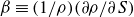
The focus of the present work is on the laminar (or quasi-laminar) regime of vertical ice-face melting (or dissolution/ablation) in ambient warmer water with and without salinity. This effort involves a combination of experiments and direct numerical simulation (DNS). Although there exists prior work where melting is driven by ambient temperature alone (i.e. freshwater), relatively less focus has been on ambient saline water – this is especially relevant to Antarctic conditions which are characterised by high salinity and low ambient temperatures. When considering early experimental works that investigated the laminar BL of a melting vertical ice face, Josberger & Martin (Reference Josberger and Martin1981) and Carey & Gebhart (Reference Carey and Gebhart1982b ) are the leading studies. Here, they identified flow regimes based on ambient temperatures and salinities. Ice-face ablation and associated BL flow dynamics are further explored under different ice-face angles and ambient environments under turbulent flow conditions in various relatively recent studies (Kerr & McConnochie Reference Kerr and McConnochie2015; Gayen, Griffiths & Kerr Reference Gayen, Griffiths and Kerr2016; McConnochie & Kerr Reference McConnochie and Kerr2016a , Reference McConnochie and Kerrb ; McConnochie et al. Reference McConnochie2018; Mondal et al. Reference Mondal, Gayen, Griffiths and Kerr2019; Sweetman et al. Reference Sweetman, Shakespeare, Stewart and McConnochie2024). However, almost no measurements of the temperature and velocity profiles exist within the BL. These are key to understanding the dynamics of the flow and melt-rate scaling. Importantly, if the flow is driven solely by either temperature or salinity, the dynamics is simpler and the flow is uni-directional. Most studies have focused on this scenario (e.g. Ostrach Reference Ostrach1952). Herein we demonstrate that under realistic Antarctic conditions both temperature and salinity play significant roles, and can lead to a bi-directional flow (e.g. Josberger & Martin Reference Josberger and Martin1981; Nilson Reference Nilson1985). Here, a salinity-driven upward flow close to the ice sheet is accompanied by a temperature-driven downward flow away from the ice sheet (see figure 1 ai for uni- and 1 aii for bi-directional flow schematics). This bi-directional flow non-trivially affects the otherwise simpler scaling of the melt rate under laminar conditions.
(a) Boundary-layer structure adjacent to an ablating vertical ice face, with (i) uni-directional flow (where temperature and/or salinity forcing are in the same direction) and (ii) bi-directional or counter-current flow (with opposing buoyancy forcing). (b) Experimental cases (see table 1) on a T–S diagram (case 1 ![]() :
:
 $S_\infty =0$
g kg−1,
$S_\infty =0$
g kg−1,
 $T_\infty =20^{\,\circ} \text{C}$
; case 2
$T_\infty =20^{\,\circ} \text{C}$
; case 2 ![]() :
:
 $S_\infty =0$
g kg−1,
$S_\infty =0$
g kg−1,
 $T_\infty =15^{\,\circ} \text{C}$
; case 3
$T_\infty =15^{\,\circ} \text{C}$
; case 3 ![]() :
:
 $S_\infty =0$
g kg−1,
$S_\infty =0$
g kg−1,
 $T_\infty =10^{\,\circ} \text{C}$
; case 4
$T_\infty =10^{\,\circ} \text{C}$
; case 4 ![]() :
:
 $S_\infty =0$
g kg−1,
$S_\infty =0$
g kg−1,
 $T_\infty =4^{\,\circ} \text{C}$
; case 5
$T_\infty =4^{\,\circ} \text{C}$
; case 5 ![]() :
:
 $S_\infty =34$
g kg−1,
$S_\infty =34$
g kg−1,
 $T_\infty =4^{\,\circ} \text{C}$
; and case 6
$T_\infty =4^{\,\circ} \text{C}$
; and case 6 ![]() :
:
 $S_\infty =34$
g kg−1,
$S_\infty =34$
g kg−1,
 $T_\infty =2^{\,\circ} \text{C}$
), and flow regimes with region I (
$T_\infty =2^{\,\circ} \text{C}$
), and flow regimes with region I (
 ${\varLambda } \lt 0$
) and region II (
${\varLambda } \lt 0$
) and region II (
 ${\varLambda } \gt 0$
). Here,
${\varLambda } \gt 0$
). Here,
 $T_\textit{md}$
(blue solid line) and
$T_\textit{md}$
(blue solid line) and
 $T_\textit{fp}$
(black solid line) represent temperature corresponding to maximum density and freezing point temperature at different salinities, respectively. (c) Density variation of freshwater (
$T_\textit{fp}$
(black solid line) represent temperature corresponding to maximum density and freezing point temperature at different salinities, respectively. (c) Density variation of freshwater (
 $S=0$
) with temperature. Symbols represent cases 1, 2, 3 and 4 (these are also presented in table 1).
$S=0$
) with temperature. Symbols represent cases 1, 2, 3 and 4 (these are also presented in table 1).

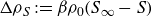
Temperature and salinity affect the flow and melt rates differently. As discussed extensively (e.g. Woods Reference Woods1992; Kerr Reference Kerr1994a , Reference Kerrb ; Wells & Worster Reference Wells and Worster2011), in cases where the diffusion caused by temperature difference between ice and ambient water is the main driver, the process is termed ‘melting’, whereas salinity-difference-driven flow is referred to as ‘dissolution’. In both cases, however, when one neglects the heat and salt transfer into the ice, the ice and melt-water interface has to satisfy the continuity of heat and salinity flux:
 \begin{align} \rho _{\textit{ice}} \textit{LV} &= \rho c_w \kappa _T \frac {\partial T}{\partial x}, \end{align}
 \begin{align} \rho _{\textit{ice}} S_i V &= \rho \kappa _S \frac {\partial S}{\partial x}. \end{align}
In (1.1) and (1.2),
 $\rho _{\textit{ice}}$
and
$\rho _{\textit{ice}}$
and
 $\rho$
are the densities of ice and water,
$\rho$
are the densities of ice and water,
 $T$
(
$T$
(
 $^{\,\circ} \text{C}$
) and
$^{\,\circ} \text{C}$
) and
 $S$
(grams of salt per kilogram of water or ‰) are temperature and salinity with
$S$
(grams of salt per kilogram of water or ‰) are temperature and salinity with
 $x$
normal to the ice and pointing into the water,
$x$
normal to the ice and pointing into the water,
 $\kappa _T$
and
$\kappa _T$
and
 $\kappa _S$
are temperature and salinity diffusivity (
$\kappa _S$
are temperature and salinity diffusivity (
 $\rm m^2\,s^{- 1}$
),
$\rm m^2\,s^{- 1}$
),
 $c_w$
and
$c_w$
and
 $L$
are the specific heat (
$L$
are the specific heat (
 $\rm J\,(\rm kg\,^{\,\circ} \text{C})^{- 1}$
) and latent heat of water (
$\rm J\,(\rm kg\,^{\,\circ} \text{C})^{- 1}$
) and latent heat of water (
 $\rm J\,kg^{- 1}$
) and
$\rm J\,kg^{- 1}$
) and
 $V$
is the melt rate (
$V$
is the melt rate (
 $\rm m\,s^{- 1}$
). The effect of the conductive heat flux into the ice is discussed in Kerr & McConnochie (Reference Kerr and McConnochie2015) and is negligible for ice temperatures close to the interface temperature. (For the experiments in this study, heat transfer into the ice is estimated to be less than
$\rm m\,s^{- 1}$
). The effect of the conductive heat flux into the ice is discussed in Kerr & McConnochie (Reference Kerr and McConnochie2015) and is negligible for ice temperatures close to the interface temperature. (For the experiments in this study, heat transfer into the ice is estimated to be less than
 $4\,\%$
of the heat required for ice melting, which has a negligible impact on the interface temperature and ice melt-rate estimations.) Note also that, at the interface,
$4\,\%$
of the heat required for ice melting, which has a negligible impact on the interface temperature and ice melt-rate estimations.) Note also that, at the interface,
 $T=T_i$
and
$T=T_i$
and
 $S=S_i$
are connected by the freezing point depression equation of saltwater:
$S=S_i$
are connected by the freezing point depression equation of saltwater:
 \begin{equation} T_i= a_s S_i , \end{equation}
where
 $a_s\approx -6 \times 10^{-2}{\rm ^\circ\, C}\,$
‰−1 (Josberger & Martin Reference Josberger and Martin1981). As a consequence of the freezing point depression equation as well as (1.1) and (1.2), when an ice face dissolves in saline water, the salinity of the water adjacent to the interface remains non-zero, even though the ice block itself is made of freshwater. The governing equations for the flow field, expressing the conservation of momentum and mass and the transport of two scalars, along with (1.1) and (1.2) govern the melt-water BL dynamics.
$a_s\approx -6 \times 10^{-2}{\rm ^\circ\, C}\,$
‰−1 (Josberger & Martin Reference Josberger and Martin1981). As a consequence of the freezing point depression equation as well as (1.1) and (1.2), when an ice face dissolves in saline water, the salinity of the water adjacent to the interface remains non-zero, even though the ice block itself is made of freshwater. The governing equations for the flow field, expressing the conservation of momentum and mass and the transport of two scalars, along with (1.1) and (1.2) govern the melt-water BL dynamics.
For single-component flow, such as temperature- or salinity-driven flow, self-similar solutions of the BL equations exist (e.g. Ostrach Reference Ostrach1952; Nilson Reference Nilson1985; Wells & Worster Reference Wells and Worster2011) whereas Nilson (Reference Nilson1985) tried to obtain some non-self-similar solutions where both temperature and salinity effects are significant. Analytical works usually assume constant properties, such as
 $\kappa _T$
and
$\kappa _T$
and
 $\kappa _S$
, and a linear variation of density dependence on temperature and salinity, although exceptions exist (e.g. Gebhart & Mollendorf Reference Gebhart and Mollendorf1977) that take into consideration the density maxima at
$\kappa _S$
, and a linear variation of density dependence on temperature and salinity, although exceptions exist (e.g. Gebhart & Mollendorf Reference Gebhart and Mollendorf1977) that take into consideration the density maxima at
 $T\approx 4^{\,\circ} \text{C}$
for low salinity. Experimental progress, however, has been limited because of the difficulty in measuring temperature (and/or salinity) and velocity distribution in water adjacent to a melting ice face. Nevertheless, limited velocity measurements have been carried out. Wilson & Vyas (Reference Wilson and Vyas1979) adopted a technique that uses a pH indicator (thymol blue) that can work as a coloured marker to track the flow; Carey & Gebhart (Reference Carey and Gebhart1982a
) and Josberger & Martin (Reference Josberger and Martin1981) estimated flow velocity using long-exposure photography of illuminated particles; and McConnochie & Kerr (Reference McConnochie and Kerr2016b
) used a shadowgraph turbulent eddy tracking technique to estimate maximum plume velocity. As far as BL temperature data are concerned, some of these studies provide ice–water interface and far-field temperatures measured using stationary thermistors or thermocouples (Bendell & Gebhart Reference Bendell and Gebhart1976; Josberger & Martin Reference Josberger and Martin1981; Carey & Gebhart Reference Carey and Gebhart1982a
; McConnochie & Kerr Reference McConnochie and Kerr2016b
; McConnochie et al. Reference McConnochie2018). However, temperature profiles across the BL flow are not available in previous studies. In all experimental studies that measured ice ablation rate, the position of the ice–water interface is obtained as a function of time, which has been used to estimate the melt rate (Josberger & Martin Reference Josberger and Martin1981; Kerr & McConnochie Reference Kerr and McConnochie2015). Obtaining velocity and temperature profile measurements within the BL has been a significant challenge because of the small measurement domain (
$T\approx 4^{\,\circ} \text{C}$
for low salinity. Experimental progress, however, has been limited because of the difficulty in measuring temperature (and/or salinity) and velocity distribution in water adjacent to a melting ice face. Nevertheless, limited velocity measurements have been carried out. Wilson & Vyas (Reference Wilson and Vyas1979) adopted a technique that uses a pH indicator (thymol blue) that can work as a coloured marker to track the flow; Carey & Gebhart (Reference Carey and Gebhart1982a
) and Josberger & Martin (Reference Josberger and Martin1981) estimated flow velocity using long-exposure photography of illuminated particles; and McConnochie & Kerr (Reference McConnochie and Kerr2016b
) used a shadowgraph turbulent eddy tracking technique to estimate maximum plume velocity. As far as BL temperature data are concerned, some of these studies provide ice–water interface and far-field temperatures measured using stationary thermistors or thermocouples (Bendell & Gebhart Reference Bendell and Gebhart1976; Josberger & Martin Reference Josberger and Martin1981; Carey & Gebhart Reference Carey and Gebhart1982a
; McConnochie & Kerr Reference McConnochie and Kerr2016b
; McConnochie et al. Reference McConnochie2018). However, temperature profiles across the BL flow are not available in previous studies. In all experimental studies that measured ice ablation rate, the position of the ice–water interface is obtained as a function of time, which has been used to estimate the melt rate (Josberger & Martin Reference Josberger and Martin1981; Kerr & McConnochie Reference Kerr and McConnochie2015). Obtaining velocity and temperature profile measurements within the BL has been a significant challenge because of the small measurement domain (
 ${\approx}1$
mm salinity BL and
${\approx}1$
mm salinity BL and
 $1{-}2$
cm thermal and velocity BL), limited options for measuring temperature and the small velocity magnitudes adjacent to a receding ice interface. Here, we have adapted the techniques of molecular tagging velocimetry (MTV) and thermometry (MTT), respectively, for velocity and temperature measurements (Gendrich, Koochesfahani & Nocera Reference Gendrich, Koochesfahani and Nocera1997; Hu & Koochesfahani Reference Hu and Koochesfahani2006; Agrawal et al. Reference Agrawal, Ramesh, Zimmerman, Philip and Klewicki2021) across the BL to the present low-temperature and velocity situation (detailed in § 3) for both far-field salinity
$1{-}2$
cm thermal and velocity BL), limited options for measuring temperature and the small velocity magnitudes adjacent to a receding ice interface. Here, we have adapted the techniques of molecular tagging velocimetry (MTV) and thermometry (MTT), respectively, for velocity and temperature measurements (Gendrich, Koochesfahani & Nocera Reference Gendrich, Koochesfahani and Nocera1997; Hu & Koochesfahani Reference Hu and Koochesfahani2006; Agrawal et al. Reference Agrawal, Ramesh, Zimmerman, Philip and Klewicki2021) across the BL to the present low-temperature and velocity situation (detailed in § 3) for both far-field salinity
 $S_\infty =0$
and
$S_\infty =0$
and
 $S_\infty = 34$
‰ corresponding to seawater and different far-field temperatures (
$S_\infty = 34$
‰ corresponding to seawater and different far-field temperatures (
 $T_\infty$
).
$T_\infty$
).
As a complement to experiments, DNS can generally provide much greater details. Owing to the complexity of the problem, however, DNS studies addressing vertical ice-face melting are sparse. Studies such as Gayen et al. (Reference Gayen, Griffiths and Kerr2016), which investigated turbulent BLs along a vertical ice face, and Mondal et al. (Reference Mondal, Gayen, Griffiths and Kerr2019), which focused on inclined ice, have previously examined ice-face ablation driven by natural convection. These include a linear equation of state (EoS) and smaller Schmidt numbers. More recently, Yang et al. (Reference Yang, Howland, Liu, Verzicco and Lohse2023) performed DNS with ambient stratification, but relatively large ambient temperature (
 $20^{\,\circ} \text{C}$
) and low salinity (up to
$20^{\,\circ} \text{C}$
) and low salinity (up to
 $15$
‰). Ice melting under laminar natural convection at realistic Antarctic conditions remains largely unexplored, and the present DNS incorporating linear as well as nonlinear EoS and other realistic non-dimensional parameters aims to fill some of this gap.
$15$
‰). Ice melting under laminar natural convection at realistic Antarctic conditions remains largely unexplored, and the present DNS incorporating linear as well as nonlinear EoS and other realistic non-dimensional parameters aims to fill some of this gap.
The objectives of this study are twofold. The first is to obtain experimental velocity and temperature profiles along with simultaneous melt-rate measurements, and carry out DNS of the same physical domain. The second objective is to study the velocity and temperature profiles as well as the melt rates and their scaling with height for a range of ambient temperatures and salinities, and thus clarify the role of opposing buoyancy arising due to temperature and salinity in the BL dynamics. The rest of this paper is organised as follows: In § 2 the relevant non-dimensional numbers and the expected flow regimes for both uni- and bi-directional flow are discussed. We also present a method to evaluate the possible flow scenarios appropriate to Antarctic conditions with only the knowledge of far-field temperature and salinity. Next, the experimental set-up and modifications to previous MTV/MTT implementations are outlined in § 3. These modifications allow us to measure low velocities as well as temperatures within the melt BL. Details of the DNS that mimic our experimental set-up are discussed in § 4. In § 5 we present the velocity and temperature data from the experiments and simulations. Finally, the melt-rate data as well as expected scalings are discussed in § 6 before the summary and conclusions are presented in § 7.
2. Governing non-dimensional numbers and relevance to Antarctic conditions
2.1. Governing non-dimensional numbers
For a single-component flow, say, driven only by the difference between ambient and interface temperature (
 $T_\infty$
and
$T_\infty$
and
 $T_i$
, respectively), the relevant non-dimensional parameters are the Prandtl and Grashof numbers:
$T_i$
, respectively), the relevant non-dimensional parameters are the Prandtl and Grashof numbers:
 \begin{equation} \textit{Pr} = \frac {\nu }{\kappa _T}\quad \textrm {and}\quad \textit{Gr}_z = \frac {z^3 g\alpha (T_\infty -T_i)}{\nu ^2}, \end{equation}
where
 $\nu$
is the kinematic viscosity of the fluid,
$\nu$
is the kinematic viscosity of the fluid,
 $z$
is the vertical distance with origin at the bottom (see figure 1
ai and 1
aii),
$z$
is the vertical distance with origin at the bottom (see figure 1
ai and 1
aii),
 $g$
is the gravitational acceleration and
$g$
is the gravitational acceleration and
 $\alpha \equiv -(1/\rho )(\partial \rho /\partial T)$
is the thermal expansion coefficient. It is also common to define
$\alpha \equiv -(1/\rho )(\partial \rho /\partial T)$
is the thermal expansion coefficient. It is also common to define
 $\textit{Gr}_H$
based on the total height of the ice face
$\textit{Gr}_H$
based on the total height of the ice face
 $H$
. Based on
$H$
. Based on
 $H=8.5$
cm for our set-up, we have
$H=8.5$
cm for our set-up, we have
 $ 3.6\times 10^6 \lessapprox \textit{Gr}_H \lessapprox 9.7\times 10^7$
and
$ 3.6\times 10^6 \lessapprox \textit{Gr}_H \lessapprox 9.7\times 10^7$
and
 $7 \lessapprox \textit{Pr} \lessapprox 13$
. Also, it is interesting to represent
$7 \lessapprox \textit{Pr} \lessapprox 13$
. Also, it is interesting to represent
 $\textit{Gr}_H$
as a ratio of viscous to buoyancy time scales:
$\textit{Gr}_H$
as a ratio of viscous to buoyancy time scales:
 $\sqrt {\textit{Gr}_H} = (H^2/\nu )/\sqrt {H/g'}$
, where reduced gravity
$\sqrt {\textit{Gr}_H} = (H^2/\nu )/\sqrt {H/g'}$
, where reduced gravity
 $g':=g\alpha (T_\infty -T_i)$
, and
$g':=g\alpha (T_\infty -T_i)$
, and
 $\sqrt [4]{\textit{Gr}_H} = H/\sqrt [4]{\nu ^2 H/g'}$
as a ratio of length scales (where the denominator is the viscous-gravity length scale
$\sqrt [4]{\textit{Gr}_H} = H/\sqrt [4]{\nu ^2 H/g'}$
as a ratio of length scales (where the denominator is the viscous-gravity length scale
 $l_T$
in (A6) without the numerical factor and
$l_T$
in (A6) without the numerical factor and
 $z \mapsto H$
). For example, in our case
$z \mapsto H$
). For example, in our case
 $1900\lessapprox \sqrt {\textit{Gr}_H} \lessapprox 9850$
and
$1900\lessapprox \sqrt {\textit{Gr}_H} \lessapprox 9850$
and
 $45 \lessapprox \sqrt [4]{\textit{Gr}_H} \lessapprox 100$
, which further highlights the importance of buoyancy.
$45 \lessapprox \sqrt [4]{\textit{Gr}_H} \lessapprox 100$
, which further highlights the importance of buoyancy.
Addition of a second component, say salinity, to the existing temperature adds two dimensional quatities:
 $S_\infty$
or the difference of far-field to interface salinity
$S_\infty$
or the difference of far-field to interface salinity
 $(S_\infty -S_i)$
and
$(S_\infty -S_i)$
and
 $\kappa _S$
, giving rise to two more non-dimensional groups:
$\kappa _S$
, giving rise to two more non-dimensional groups:
 \begin{equation} {\varLambda } \equiv \frac {\alpha \rho _0 (T_\infty -T_i)}{\beta \rho _0(S_\infty -S_i)}=\frac {\Delta \rho _T}{\Delta \rho _S}\quad\textrm {and}\quad \textit{Sc} = \frac {\nu }{\kappa _S}\quad\textrm {or}\quad \textit{Le} = \frac {\kappa _T}{\kappa _S}. \end{equation}
These are, respectively, the ratio of density changes owing to temperature and salinity, and Schmidt and Lewis numbers, where
 $\beta \equiv (1/\rho )(\partial \rho /\partial S)$
is the haline contraction coefficient and
$\beta \equiv (1/\rho )(\partial \rho /\partial S)$
is the haline contraction coefficient and
 $\rho _0$
is reference density. For our cases
$\rho _0$
is reference density. For our cases
 ${\varLambda }\approx 1/40$
,
${\varLambda }\approx 1/40$
,
 $\textit{Sc}\approx 2000$
and
$\textit{Sc}\approx 2000$
and
 $\textit{Le} \approx 200$
.
$\textit{Le} \approx 200$
.
For nonlinear density variations, Gebhart & Mollendorf (Reference Gebhart and Mollendorf1977) and Carey & Gebhart (Reference Carey and Gebhart1982b ) introduced another non-dimensional number:
 \begin{equation} R = \frac {T_\textit{md}(S_\infty )-T_\infty }{T_i-T_\infty }, \end{equation}
where
 $T_\textit{md}$
is the temperature where the maximum density occurs. Parameter
$T_\textit{md}$
is the temperature where the maximum density occurs. Parameter
 $R$
is a stronger function of salinity at lower
$R$
is a stronger function of salinity at lower
 $S$
(see figure 1
b and 1
c). This is because, at low
$S$
(see figure 1
b and 1
c). This is because, at low
 $S$
, the value of
$S$
, the value of
 $T_\textit{md}$
deviates significantly from
$T_\textit{md}$
deviates significantly from
 $T_i$
as
$T_i$
as
 $S$
decreases and it provides an indirect measure of how significant the nonlinear effects of temperature are on the density for a given
$S$
decreases and it provides an indirect measure of how significant the nonlinear effects of temperature are on the density for a given
 $T_i$
and
$T_i$
and
 $T_\infty$
. Further,
$T_\infty$
. Further,
 $R$
is useful to predict the direction of flow for different ambient conditions when interface conditions are known (Gebhart & Jaluria Reference Gebhart and Jaluria1988), especially for low-salinity cases. These flow regimes are now discussed.
$R$
is useful to predict the direction of flow for different ambient conditions when interface conditions are known (Gebhart & Jaluria Reference Gebhart and Jaluria1988), especially for low-salinity cases. These flow regimes are now discussed.
2.2. Flow regimes
When an ice face is in contact with saline water, the water adjacent to the ice–water interface is subjected to cooling and dilution. Cooling induces a thermal BL within which the temperature varies from the freezing point temperature
 $T_\textit{fp}(S_i)$
(shown in figure 1
b) to the ambient water temperature (
$T_\textit{fp}(S_i)$
(shown in figure 1
b) to the ambient water temperature (
 $T_\infty$
). Owing to dilution, a salinity BL forms where water gets less saline closer to the ice due to freshwater released from the melting ice. These thermal and saline BLs are depicted in figure 1(ai) and 1(aii). Importantly, since salt has very low diffusivity compared with heat (
$T_\infty$
). Owing to dilution, a salinity BL forms where water gets less saline closer to the ice due to freshwater released from the melting ice. These thermal and saline BLs are depicted in figure 1(ai) and 1(aii). Importantly, since salt has very low diffusivity compared with heat (
 $\textit{Le} =\kappa _T/\kappa _S \approx 200$
), the saline BL thickness (
$\textit{Le} =\kappa _T/\kappa _S \approx 200$
), the saline BL thickness (
 $\delta _S$
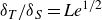
) is about 14 times smaller (assuming
$\delta _S$
) is about 14 times smaller (assuming
 $\delta _S/\delta _T\approx \textit{Le}^{-1/2}$
, which is discussed in § 6) compared with the thickness of the thermal BL (
$\delta _S/\delta _T\approx \textit{Le}^{-1/2}$
, which is discussed in § 6) compared with the thickness of the thermal BL (
 $\delta _T$
). Although the contribution of salinity to the change in density is large compared with the temperature (
$\delta _T$
). Although the contribution of salinity to the change in density is large compared with the temperature (
 ${\varLambda }\approx 1/40$
), owing to the low diffusivity of salt, density variations due to salt only affect a very thin layer of water closest to the interface. On the other hand, despite having a relatively small contribution to the density variation, the thermal BL affects density variations across a broader domain than the salinity BL.
${\varLambda }\approx 1/40$
), owing to the low diffusivity of salt, density variations due to salt only affect a very thin layer of water closest to the interface. On the other hand, despite having a relatively small contribution to the density variation, the thermal BL affects density variations across a broader domain than the salinity BL.
Josberger & Martin (Reference Josberger and Martin1981) used experiments and existing similarity solutions to map the BL forming next to a melting vertical ice face. The mapping was carried out on a temperature–salinity (
 $T_\infty ,\,S_\infty$
) diagram like that shown in figure 1(b). Although the map was prepared mostly for turbulent flows, as discussed later, some features are relevant for laminar flows. Importantly, we draw connections between this map on the (
$T_\infty ,\,S_\infty$
) diagram like that shown in figure 1(b). Although the map was prepared mostly for turbulent flows, as discussed later, some features are relevant for laminar flows. Importantly, we draw connections between this map on the (
 $T_\infty ,\,S_\infty )$
plane and the more informative non-dimensional
$T_\infty ,\,S_\infty )$
plane and the more informative non-dimensional
 $({\varLambda },\,\textit{Le})$
plane description of Nilson (Reference Nilson1985).
$({\varLambda },\,\textit{Le})$
plane description of Nilson (Reference Nilson1985).
In figure 1(b), the temperature at maximum density for each salinity is the line
 $T_\textit{md}$
(in blue colour, where
$T_\textit{md}$
(in blue colour, where
 $R=0$
; equation (2.3)) and the freezing point temperature line is
$R=0$
; equation (2.3)) and the freezing point temperature line is
 $T_\textit{fp}$
(in black colour) that separates the ice and water states. Depending on where
$T_\textit{fp}$
(in black colour) that separates the ice and water states. Depending on where
 $T_\infty$
and
$T_\infty$
and
 $S_\infty$
lie on the T–S diagram, Josberger & Martin (Reference Josberger and Martin1981) report different BL regimes. When the ambient conditions are in region I, enclosed by
$S_\infty$
lie on the T–S diagram, Josberger & Martin (Reference Josberger and Martin1981) report different BL regimes. When the ambient conditions are in region I, enclosed by
 $T_\textit{md}$
and
$T_\textit{md}$
and
 $T_\textit{fp}$
,
$T_\textit{fp}$
,
 $\varLambda$
is negative. This is because
$\varLambda$
is negative. This is because
 $\Delta \rho _T := \alpha \rho _0 (T_\infty -T)$
is negative as
$\Delta \rho _T := \alpha \rho _0 (T_\infty -T)$
is negative as
 $\alpha$
is negative in this region, and
$\alpha$
is negative in this region, and
 $\Delta \rho _S:= {\beta } \rho _0 (S_\infty -S)$
is always positive because freshwater is always less dense relative to saltwater at the same temperature. That is, both salt and temperature produce less dense water, favouring an upward uni-directional BL flow. Due to this uniformity of the flow, similarity solutions exist for the laminar BL equations in this region (see (A1a
) and (A1b
)).
$\Delta \rho _S:= {\beta } \rho _0 (S_\infty -S)$
is always positive because freshwater is always less dense relative to saltwater at the same temperature. That is, both salt and temperature produce less dense water, favouring an upward uni-directional BL flow. Due to this uniformity of the flow, similarity solutions exist for the laminar BL equations in this region (see (A1a
) and (A1b
)).
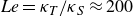
(a) Relative buoyancy–diffusivity diagram (
 $\varLambda {-}\textit{Le}$
) showing flow regimes. Here (
$\varLambda {-}\textit{Le}$
) showing flow regimes. Here (![]() )
)
 $\varLambda \textit{Le}= 1$
, (
$\varLambda \textit{Le}= 1$
, (![]() )
)
 $\varLambda \textit{Le}^{1/2} = 1$
and (
$\varLambda \textit{Le}^{1/2} = 1$
and (![]() )
)
 $\varLambda \textit{Le}^{1/3} = 1$
. Contours represent
$\varLambda \textit{Le}^{1/3} = 1$
. Contours represent
 $\varLambda \textit{Le}^{1/2}$
. Symbols: filled
$\varLambda \textit{Le}^{1/2}$
. Symbols: filled
 $\diamond$
and filled
$\diamond$
and filled
 $\vartriangleleft$
show experimental data for cases 5 and 6, respectively. Also shown are laminar bi-directional experimental results of Josberger & Martin (Reference Josberger and Martin1981) in filled yellow
$\vartriangleleft$
show experimental data for cases 5 and 6, respectively. Also shown are laminar bi-directional experimental results of Josberger & Martin (Reference Josberger and Martin1981) in filled yellow
 $\triangledown$
and of Carey & Gebhart (Reference Carey and Gebhart1982a
) in filled green
$\triangledown$
and of Carey & Gebhart (Reference Carey and Gebhart1982a
) in filled green
 $\triangle$
for comparison. Analytical values of
$\triangle$
for comparison. Analytical values of
 $\varLambda$
obtained using (2.6) are shown in the colour bar for ambient temperatures
$\varLambda$
obtained using (2.6) are shown in the colour bar for ambient temperatures
 $T_\infty =-2^{\,\circ} \text{C}$
to
$T_\infty =-2^{\,\circ} \text{C}$
to
 $4^{\,\circ} \text{C}$
(blue to red colour) expected in the context of Antarctic ice melting with higher (lower) temperatures in red (blue). (b) Zoomed-in view of (a). (c) Temperature
$4^{\,\circ} \text{C}$
(blue to red colour) expected in the context of Antarctic ice melting with higher (lower) temperatures in red (blue). (b) Zoomed-in view of (a). (c) Temperature
 $T_i$
obtained from solving (2.6) for different ambient conditions (labels on the curves denote salinity). Also shown are the experimental results of Carey & Gebhart (Reference Carey and Gebhart1982a
) (filled green
$T_i$
obtained from solving (2.6) for different ambient conditions (labels on the curves denote salinity). Also shown are the experimental results of Carey & Gebhart (Reference Carey and Gebhart1982a
) (filled green
 $\triangle$
) and numerical results of Carey & Gebhart (Reference Carey and Gebhart1982b
) (open green
$\triangle$
) and numerical results of Carey & Gebhart (Reference Carey and Gebhart1982b
) (open green
 $\triangle$
) for
$\triangle$
) for
 $S_\infty = 10$
g kg−1. The experimental data of Josberger & Martin (Reference Josberger and Martin1981) are indicated by filled yellow
$S_\infty = 10$
g kg−1. The experimental data of Josberger & Martin (Reference Josberger and Martin1981) are indicated by filled yellow
 $\triangledown$
(for
$\triangledown$
(for
 $S_\infty = 34.4$
g kg−1). The DNS results of this study for case 5 and case 6 are shown as open
$S_\infty = 34.4$
g kg−1). The DNS results of this study for case 5 and case 6 are shown as open
 $\diamond$
and
$\diamond$
and
 $\vartriangleleft$
, respectively (both for
$\vartriangleleft$
, respectively (both for
 $S_\infty = 34$
g kg−1).
$S_\infty = 34$
g kg−1).

When the ambient condition shifts into region II, having a high salinity and relatively low temperature,
 $\Delta \rho _T$
gradually becomes negative, resulting in
$\Delta \rho _T$
gradually becomes negative, resulting in
 ${\varLambda } \gt 0$
. In this region, buoyancy forces from salinity (closer to the wall) and temperature (farther from the wall) oppose each other. This can result in bi-directional or counter-current flows. However, Carey & Gebhart (Reference Carey and Gebhart1982b
) showed through numerical calculations that even with opposing buoyancy forces, uni-directional upward flow can exist for some cases within the region where the salinity buoyancy force dominates over the thermal buoyancy force. This shows that the limits of counter-current flow are less apparent on a
${\varLambda } \gt 0$
. In this region, buoyancy forces from salinity (closer to the wall) and temperature (farther from the wall) oppose each other. This can result in bi-directional or counter-current flows. However, Carey & Gebhart (Reference Carey and Gebhart1982b
) showed through numerical calculations that even with opposing buoyancy forces, uni-directional upward flow can exist for some cases within the region where the salinity buoyancy force dominates over the thermal buoyancy force. This shows that the limits of counter-current flow are less apparent on a
 $T_\infty {-} S_\infty$
diagram. Nilson (Reference Nilson1985) obtained these limits on the
$T_\infty {-} S_\infty$
diagram. Nilson (Reference Nilson1985) obtained these limits on the
 $({\varLambda },\,\textit{Le})$
plane as shown in figure 2(a). Starting with a dominant upwards salinity-driven flow, an incipient temperature-driven downward flow (i.e. an overall bi-directional flow) appears when
$({\varLambda },\,\textit{Le})$
plane as shown in figure 2(a). Starting with a dominant upwards salinity-driven flow, an incipient temperature-driven downward flow (i.e. an overall bi-directional flow) appears when
 ${\varLambda } \textit{Le}\approx 1$
. If, however, there is a dominant temperature-driven downward flow an incipient salinity-driven upward flow adjacent to the wall will result when
${\varLambda } \textit{Le}\approx 1$
. If, however, there is a dominant temperature-driven downward flow an incipient salinity-driven upward flow adjacent to the wall will result when
 ${\varLambda } \textit{Le}^{1/3} \approx 1$
. Appendix A provides a derivation of these limits starting from the BL equations. These limits of upward and downward flows are presented in figure 2(a). They divide the
${\varLambda } \textit{Le}^{1/3} \approx 1$
. Appendix A provides a derivation of these limits starting from the BL equations. These limits of upward and downward flows are presented in figure 2(a). They divide the
 $({\varLambda },\,\textit{Le})$
plane into three regions: up-flow; counter-flow or bi-directional flow; and down-flow.
$({\varLambda },\,\textit{Le})$
plane into three regions: up-flow; counter-flow or bi-directional flow; and down-flow.
An estimate of the demarcating line between the upward saline-buoyancy-dominated and the downward thermal-buoyancy-dominated regimes can be obtained quite straightforwardly by evaluating the relative buoyancy strengths. Net buoyancy is not governed only by
 $\Delta \rho _T$
and
$\Delta \rho _T$
and
 $\Delta \rho _S$
, i.e.
$\Delta \rho _S$
, i.e.
 $\varLambda$
, rather by the density difference acting over the respective BL thickness
$\varLambda$
, rather by the density difference acting over the respective BL thickness
 $\delta _T$
and
$\delta _T$
and
 $\delta _S$
. Therefore, it is the ratio
$\delta _S$
. Therefore, it is the ratio
 \begin{equation} \frac {\Delta \rho _T \,\delta _T}{\Delta \rho _S\,\delta _S}\sim {\varLambda } \textit{Le}^{1/2} \end{equation}
that determines the relative strength of temperature and salinity within the BL. Not surprisingly, the line
 ${\varLambda } \textit{Le}^{1/2}$
bisects the bi-directional flow region in figure 2(a) as shown in the blue dashed line. In figure 2(a), we compare the experimental results of Josberger & Martin (Reference Josberger and Martin1981) and Carey & Gebhart (Reference Carey and Gebhart1982a
), where laminar bi-directional or marginally bi-directional flows were observed, in the
${\varLambda } \textit{Le}^{1/2}$
bisects the bi-directional flow region in figure 2(a) as shown in the blue dashed line. In figure 2(a), we compare the experimental results of Josberger & Martin (Reference Josberger and Martin1981) and Carey & Gebhart (Reference Carey and Gebhart1982a
), where laminar bi-directional or marginally bi-directional flows were observed, in the
 $\varLambda$
–
$\varLambda$
–
 $\textit{Le}$
plane. As shown in the figure, these data fall within the region corresponding to counter-flow, providing confidence in the validity of the formulation.
$\textit{Le}$
plane. As shown in the figure, these data fall within the region corresponding to counter-flow, providing confidence in the validity of the formulation.
Since natural convection adjacent to Antarctic ice shelves is one of the motivations of the present work, in the following we estimate the locations of Antarctic data within the
 $({\varLambda },\,\textit{Le})$
plane in figure 2(a).
$({\varLambda },\,\textit{Le})$
plane in figure 2(a).
2.3. Laminar flow at Antarctic conditions
Only
 $T_\infty$
and
$T_\infty$
and
 $S_\infty$
conditions are known for Antarctic conditions. If, however, one can estimate
$S_\infty$
conditions are known for Antarctic conditions. If, however, one can estimate
 $T_i$
and
$T_i$
and
 $S_i$
,
$S_i$
,
 $\varLambda$
and
$\varLambda$
and
 $\textit{Le}$
can be estimated. Towards this end, we assume that within the laminar BL both temperature and salinity vary linearly across the respective BLs, and, therefore, (1.1) and (1.2) can be written in terms of interface and far-field conditions:
$\textit{Le}$
can be estimated. Towards this end, we assume that within the laminar BL both temperature and salinity vary linearly across the respective BLs, and, therefore, (1.1) and (1.2) can be written in terms of interface and far-field conditions:
 \begin{equation} \rho _{\textit{ice}} L V \approx \rho _w c_w \kappa _T \frac {(T_\infty -T_i)}{\delta _T}\quad \textrm {and}\quad \rho _{\textit{ice}} S_i V \approx \rho _w \kappa _S \frac {(S_\infty -S_i)}{\delta _S}. \end{equation}
Dividing the above two equations, substituting
 $({\delta _T}/{\delta _S})^2 = {\kappa _T}/{\kappa _S}$
and replacing
$({\delta _T}/{\delta _S})^2 = {\kappa _T}/{\kappa _S}$
and replacing
 $S_i$
with freezing point depression
$S_i$
with freezing point depression
 $T_i/a_s$
results in
$T_i/a_s$
results in
 \begin{equation} T_i^2\left (\frac {\textit{Le}^{1/2} c_w}{a_s L}\right ) -T_i\! \left (\frac {1}{a_s} +\frac {\textit{Le}^{1/2} c_w T_\infty }{a_s L}\right ) + S_\infty =0. \end{equation}
The above quadratic equation can be solved for
 $T_i$
(and hence
$T_i$
(and hence
 $S_i$
) by knowing the other quantities. In passing we note that a quadratic equation for
$S_i$
) by knowing the other quantities. In passing we note that a quadratic equation for
 $S_i$
for turbulent flow (using different assumptions) is obtained by McPhee, Morison & Nilsen (Reference McPhee, Morison and Nilsen2008). The approximate values of
$S_i$
for turbulent flow (using different assumptions) is obtained by McPhee, Morison & Nilsen (Reference McPhee, Morison and Nilsen2008). The approximate values of
 $\kappa _T=1.4\times 10^{-7}$
(Nayar et al. Reference Nayar, Panchanathan, McKinley and Lienhard2014) and
$\kappa _T=1.4\times 10^{-7}$
(Nayar et al. Reference Nayar, Panchanathan, McKinley and Lienhard2014) and
 $\kappa _S=7\times 10^{-10}$
(Caldwell Reference Caldwell1974) give
$\kappa _S=7\times 10^{-10}$
(Caldwell Reference Caldwell1974) give
 $\textit{Le}=200$
. The roots of (2.6) between
$\textit{Le}=200$
. The roots of (2.6) between
 $0$
and
$0$
and
 $a_s S_\infty$
are plotted in figure 2(c) along with some existing data for different salinities (Josberger & Martin Reference Josberger and Martin1981; Carey & Gebhart Reference Carey and Gebhart1982a
,
Reference Carey and Gebhartb
). These show a reasonable agreement between the solution of (2.6) and the data. Note that this root is always zero for the freshwater case (
$a_s S_\infty$
are plotted in figure 2(c) along with some existing data for different salinities (Josberger & Martin Reference Josberger and Martin1981; Carey & Gebhart Reference Carey and Gebhart1982a
,
Reference Carey and Gebhartb
). These show a reasonable agreement between the solution of (2.6) and the data. Note that this root is always zero for the freshwater case (
 $S_\infty =0$
). For saltwater,
$S_\infty =0$
). For saltwater,
 $T_i$
increases with increasing
$T_i$
increases with increasing
 $T_\infty$
. Further, for a given
$T_\infty$
. Further, for a given
 $T_\infty$
,
$T_\infty$
,
 $T_i$
decreases with increasing
$T_i$
decreases with increasing
 $S_\infty$
. We should mention that the validity of the assumption
$S_\infty$
. We should mention that the validity of the assumption
 $\delta _T / \delta _S = \textit{Le}^{1/2}$
leading to (2.6) may not be theoretically accurate under certain ambient conditions where the flow becomes bi-directional resulting in two distinct velocity scales within the BL, as discussed further in § 6. However, as shown in figure 2(c), the formulation in (2.6) is able to reproduce both numerical and experimental observations, even when the flow becomes bi-directional (because the two aforementioned velocity scales are of similar magnitude; see § 6).
$\delta _T / \delta _S = \textit{Le}^{1/2}$
leading to (2.6) may not be theoretically accurate under certain ambient conditions where the flow becomes bi-directional resulting in two distinct velocity scales within the BL, as discussed further in § 6. However, as shown in figure 2(c), the formulation in (2.6) is able to reproduce both numerical and experimental observations, even when the flow becomes bi-directional (because the two aforementioned velocity scales are of similar magnitude; see § 6).
At Antarctic ice shelves, the water temperature can range from approximately
 $2 ^{\,\circ} \text{C}$
to
$2 ^{\,\circ} \text{C}$
to
 $-2^{\,\circ} \text{C}$
(Jenkins et al. Reference Jenkins, Dutrieux, Jacobs, McPhail, Perrett, Webb and White2010; Boehme & Rosso Reference Boehme and Rosso2021). The values of
$-2^{\,\circ} \text{C}$
(Jenkins et al. Reference Jenkins, Dutrieux, Jacobs, McPhail, Perrett, Webb and White2010; Boehme & Rosso Reference Boehme and Rosso2021). The values of
 $\varLambda$
estimated for this condition are plotted in figure 2(a) using colour ranging from blue to red corresponding to
$\varLambda$
estimated for this condition are plotted in figure 2(a) using colour ranging from blue to red corresponding to
 $T_\infty =-2^{\,\circ} \text{C}$
to
$T_\infty =-2^{\,\circ} \text{C}$
to
 $4 ^{\,\circ} \text{C}$
. A zoomed-in view is given in figure 2(b). The values lie in the inner-dominated bi-directional or counter-flow region for this entire temperature range. Also, as
$4 ^{\,\circ} \text{C}$
. A zoomed-in view is given in figure 2(b). The values lie in the inner-dominated bi-directional or counter-flow region for this entire temperature range. Also, as
 $T_\infty$
decreases, the data deviate from the
$T_\infty$
decreases, the data deviate from the
 ${\varLambda } \textit{Le}^{1/2}$
line and become more inner-dominated. Note that figure 2(a) also shows two of our laboratory experimental data in symbols (see table 1, cases 5 and 6).
${\varLambda } \textit{Le}^{1/2}$
line and become more inner-dominated. Note that figure 2(a) also shows two of our laboratory experimental data in symbols (see table 1, cases 5 and 6).
We now proceed to present these laboratory experiments, and especially the modifications made to the MTV/MTT technique allowing us to measure temperature and velocity in the ice-melt BL.
3. Experimental set-up and adaptation of MTV/MTT technique
3.1. Experimental set-up
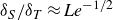
The experiments are performed in a small water tank with
 $9$
cm depth and a square base of
$9$
cm depth and a square base of
 $18$
cm in length and width (figure 3
a). One sidewall of the tank consists of a fused silica window to allow the ultraviolet (UV) laser beam needed for MTV to enter the tank. At the beginning of the experiments, an 85 mm high and 35 mm thick ice block spanning the width of the tank is placed at one end of the tank (figure 3
b), and magnets are used to secure the ice block to the endwall.
$18$
cm in length and width (figure 3
a). One sidewall of the tank consists of a fused silica window to allow the ultraviolet (UV) laser beam needed for MTV to enter the tank. At the beginning of the experiments, an 85 mm high and 35 mm thick ice block spanning the width of the tank is placed at one end of the tank (figure 3
b), and magnets are used to secure the ice block to the endwall.
Experimental cases. The far-field conditions (
 $T_\infty$
and
$T_\infty$
and
 $S_\infty$
) and environments for which these experiments are performed, as well as symbols used for each case.
$S_\infty$
) and environments for which these experiments are performed, as well as symbols used for each case.

(a) Schematic diagram of the experimental set-up and the arrangement of its components. (b) Schematic of the water tank and ice block.

As schematically shown in figure 3(a), the full experimental set-up mainly consists of the water tank, a pulsed UV laser and an intensified gated camera. A digital delay generator is used to synchronise the camera and the laser. The laser beam is guided to the fused silica window using an optics arrangement consisting of UV mirrors, and a pinhole arrangement is used to obtain a thin laser line. Images captured by the camera are logged using a host computer. Experiments with low-temperature conditions (below
 $4^\circ\, \textrm{C}$
) are performed in a temperature-controlled room (not shown here) where temperature can be maintained at a constant value ranging from
$4^\circ\, \textrm{C}$
) are performed in a temperature-controlled room (not shown here) where temperature can be maintained at a constant value ranging from
 $-15^{\,\circ} \text{C}$
to
$-15^{\,\circ} \text{C}$
to
 $25^{\,\circ} \text{C}$
.
$25^{\,\circ} \text{C}$
.
3.2. Flow measurement techniques
Measuring the velocity and temperature in the BL flow that forms next to the phase-change ice–water interface with high resolution is challenging for several reasons. Firstly, the thickness of this BL flow is small (of the order of a millimetre), and measurements have to be within (and adjacent to) this BL. Secondly, this BL flow is formed as a result of a free convection process, and, consequently, the velocities are small, about a few mm s−1. This enforces stringent requirements on the measurement system if we acknowledge that simultaneous velocity and temperature measurements are required.
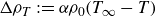
(ai) An image pair captured by the camera with
 $11$
ms interframe delay. First image with 1 ms and second image with 2 ms camera exposure. (aii) Timing chart for phosphorescence intensity (
$11$
ms interframe delay. First image with 1 ms and second image with 2 ms camera exposure. (aii) Timing chart for phosphorescence intensity (
 $I$
) decay and image pair acquisition. Here,
$I$
) decay and image pair acquisition. Here,
 $t_0$
is the time between the laser pulse and first image acquisition,
$t_0$
is the time between the laser pulse and first image acquisition,
 $\Delta t$
is interframe delay,
$\Delta t$
is interframe delay,
 $\delta t_1$
is first image exposure and
$\delta t_1$
is first image exposure and
 $\delta t_2$
is second image exposure with
$\delta t_2$
is second image exposure with
 $t_0 \ll \Delta t$
. (b) Molecular tagging melt-rate measurements – tagged line intensities.
$t_0 \ll \Delta t$
. (b) Molecular tagging melt-rate measurements – tagged line intensities.

Considering the above requirements in this study, MTV and MTT are selected. The main advantage of these molecular tagging techniques is that they use molecules as tracers (e.g. Hu & Koochesfahani Reference Hu and Koochesfahani2006), enabling them to be used to obtain measurements close to the interface with high resolution. Furthermore, in this study, the standard MTV/MTT technique is modified to obtain temperature profiles in the BL flow for simultaneously measuring small velocities. Modifications to the standard MTV/MTT implementation adopted in this study are presented later in this section.
Briefly, MTV uses phosphorescent molecules excited by a UV laser as a Lagrangian tracer, and velocities are determined by two images separated by a specified delay time as acquired by a gated intensified camera. On the other hand, MTT leverages the fact that the decay rate of the phosphorescence is uniquely temperature-dependent. In this study for both MTV and MTT, a phosphorescent supramolecular complex is used as a molecular tracer. This complex consists of 1-bromonaphthalene (1-BrNp), a certain alcohol (cyclohexanol) and an aqueous solution of maltosyl-β-cyclodextrin (Mβ-CD). In this triplex, 1-BrNp acts as the luminophore while cyclohexanol and cyclodextrin insulate the luminophore from oxygen quenching and thus generating long-lived phosphorescence (Gendrich et al. Reference Gendrich, Koochesfahani and Nocera1997). For the present study,
 $1 \times 10^{-5}\,\rm M$
molar concentration of 1-BrNp is used while the molar concentrations of cyclohexanol and cyclodextrin are
$1 \times 10^{-5}\,\rm M$
molar concentration of 1-BrNp is used while the molar concentrations of cyclohexanol and cyclodextrin are
 $0.05 \,\rm M$
and
$0.05 \,\rm M$
and
 $3 \times 10^{-4}\,\rm M$
, respectively. A 308 nm excimer laser is used for excitation for the higher-temperature cases, and a 266 nm Nd:YAG laser for temperatures of
$3 \times 10^{-4}\,\rm M$
, respectively. A 308 nm excimer laser is used for excitation for the higher-temperature cases, and a 266 nm Nd:YAG laser for temperatures of
 $4^\circ$
C or below for the cold-room experiments. The choice is merely due to convenience; and although a 308 nm excimer laser was preferred owing to higher power, it is not portable and could not be located closer to the cold room. A Princeton Instruments PI-max4 1024i intensified gated camera that captures five frames per second (2.5 image pairs per second) with an image resolution of
$4^\circ$
C or below for the cold-room experiments. The choice is merely due to convenience; and although a 308 nm excimer laser was preferred owing to higher power, it is not portable and could not be located closer to the cold room. A Princeton Instruments PI-max4 1024i intensified gated camera that captures five frames per second (2.5 image pairs per second) with an image resolution of
 $1024\times 1024$
pixels is used for image acquisition.
$1024\times 1024$
pixels is used for image acquisition.
Figure 4(ai) shows a sample phosphorescent image pair used to acquire velocity and temperature. The laser enters from the right of the image and stops after impinging on the ice surface close to the left edge. The vertical pixel displacement of the maximum intensity pixels along the line is used to calculate the Lagrangian displacement of the tracer molecules. From the knowledge of displacement and time delay, the vertical velocity profile is obtained.
Once phosphorescent molecules are excited by the UV laser beam, phosphorescent intensity decays exponentially with time, as shown in figure 4(aii). This decay can be characterised by the time constant of the decay, i.e. phosphorescent lifetime
 $(\tau )$
, which depends on the temperature. In the standard MTT technique
$(\tau )$
, which depends on the temperature. In the standard MTT technique
 $\tau$
is calculated from phosphorescence signals collected from the two images taken a time
$\tau$
is calculated from phosphorescence signals collected from the two images taken a time
 $\Delta t$
apart:
$\Delta t$
apart:
 $\tau = \Delta t/(\ln (S_1/S_2))$
, where
$\tau = \Delta t/(\ln (S_1/S_2))$
, where
 $S_1$
and
$S_1$
and
 $S_2$
are image 1 and 2 intensities taken with the same exposure time
$S_2$
are image 1 and 2 intensities taken with the same exposure time
 $\delta t$
. In our case, where velocities are small (
$\delta t$
. In our case, where velocities are small (
 $\lessapprox 8$
mm s−1), we require larger
$\lessapprox 8$
mm s−1), we require larger
 $\Delta t$
for sufficient pixel displacement (at least 5 pixels) to obtain velocity in MTV. This implies that the second image intensity
$\Delta t$
for sufficient pixel displacement (at least 5 pixels) to obtain velocity in MTV. This implies that the second image intensity
 $S_2$
will be too small (within the noise) to be useful as the phosphorescence intensity decays exponentially. To overcome this, the
$S_2$
will be too small (within the noise) to be useful as the phosphorescence intensity decays exponentially. To overcome this, the
 $S_2$
camera exposure time (
$S_2$
camera exposure time (
 $\delta t_2$
) is increased compared with the
$\delta t_2$
) is increased compared with the
 $S_1$
exposure time (
$S_1$
exposure time (
 $\delta t_1$
) needed to obtain velocities. This, however, implies that we cannot use the standard MTT methodology, because
$\delta t_1$
) needed to obtain velocities. This, however, implies that we cannot use the standard MTT methodology, because
 $\delta t_1 \neq \delta t_2$
. Thus, the MTT equation is modified as follows. A phosphorescence signal
$\delta t_1 \neq \delta t_2$
. Thus, the MTT equation is modified as follows. A phosphorescence signal
 $S$
, collected by a camera for a shutter opening at time
$S$
, collected by a camera for a shutter opening at time
 $t_0$
(after the laser is fired), is exposed for a time
$t_0$
(after the laser is fired), is exposed for a time
 $\delta t$
given by
$\delta t$
given by
 $S=\int _{t_0}^{t_0+\delta t} I_0 {\rm e}^{-t/\tau } \,$
d
$S=\int _{t_0}^{t_0+\delta t} I_0 {\rm e}^{-t/\tau } \,$
d
 $t$
, where
$t$
, where
 $I_0$
is the initial light intensity at time
$I_0$
is the initial light intensity at time
 $t_0$
. This yields
$t_0$
. This yields
 $S= I_0 \tau (1-{\rm e}^{-\delta t/\tau }){\rm e}^{-t_0/\tau }$
. Using the two signals (
$S= I_0 \tau (1-{\rm e}^{-\delta t/\tau }){\rm e}^{-t_0/\tau }$
. Using the two signals (
 $S_1$
and
$S_1$
and
 $S_2$
) from the two images separated by the interframe delay,
$S_2$
) from the two images separated by the interframe delay,
 $\Delta t$
, the phosphorescent lifetime (
$\Delta t$
, the phosphorescent lifetime (
 $\tau$
) is then obtained using
$\tau$
) is then obtained using
 \begin{equation} \frac {S_2}{S_1}= \left (\frac {1-{{\rm e}}^{{-\delta t_2}/{\tau } }}{1-\textrm {e}^{{-\delta t_1}/{\tau } }}\right ) {{\rm e}}^{{-\Delta t}/{\tau } }, \quad \textrm {where} \quad \delta t_2 \gt \delta t_1. \end{equation}
See also figure 4(aii), where
 $t_0$
is the time between the laser pulse and first image acquisition,
$t_0$
is the time between the laser pulse and first image acquisition,
 $\Delta t$
is interframe delay,
$\Delta t$
is interframe delay,
 $\delta t_1$
is first image exposure and
$\delta t_1$
is first image exposure and
 $\delta t_2$
is second image exposure with
$\delta t_2$
is second image exposure with
 $t_0 \ll \Delta t$
. Note that when
$t_0 \ll \Delta t$
. Note that when
 $\delta t_2 = \delta t_1$
, (3.1) reverts to the standard MTT equation discussed above. Equation (3.1) is numerically solved to determine
$\delta t_2 = \delta t_1$
, (3.1) reverts to the standard MTT equation discussed above. Equation (3.1) is numerically solved to determine
 $\tau$
. These
$\tau$
. These
 $\tau$
values are then converted to the temperature profile using a calibration curve, where MTT images are obtained across a range of known temperatures. This calibration procedure is described in Appendix C.
$\tau$
values are then converted to the temperature profile using a calibration curve, where MTT images are obtained across a range of known temperatures. This calibration procedure is described in Appendix C.
3.3. Making bubble-free ice
The ice is created in an acrylic mould using slightly heated water (of approximately
 $70^{\,\circ} \text{C}$
to reduce bubble formation) and keeping it in a freezer typically overnight. Once the ice is frozen, small layers of sufficiently diluted phosphorescent chemical solution are poured on the ice face (where melting happens) and allowed to freeze again. This ensures that when the ice melts, the melt plume solution emits sufficiently strong MTV and MTT signals during the experiments. Since the MTV chemical molecules can lower the freezing point of ice, a freezing point depression calculation is carried out as detailed in Appendix B. This shows that the MTV chemicals do not cause freezing point depression of more than
$70^{\,\circ} \text{C}$
to reduce bubble formation) and keeping it in a freezer typically overnight. Once the ice is frozen, small layers of sufficiently diluted phosphorescent chemical solution are poured on the ice face (where melting happens) and allowed to freeze again. This ensures that when the ice melts, the melt plume solution emits sufficiently strong MTV and MTT signals during the experiments. Since the MTV chemical molecules can lower the freezing point of ice, a freezing point depression calculation is carried out as detailed in Appendix B. This shows that the MTV chemicals do not cause freezing point depression of more than
 $0.1^{\,\circ} \text{C}$
. Furthermore, freezing thin layers of water reduces the chances of entrapped air bubbles as the freezing predominantly takes place from the bottom and the thickness of the layers cannot accommodate large bubbles. However, introducing these layers with MTV chemicals makes the ice block slightly opaque as can be seen in figure 12(ci) and 12(cii). After removing the ice block from the mould, a slightly warm (approximately
$0.1^{\,\circ} \text{C}$
. Furthermore, freezing thin layers of water reduces the chances of entrapped air bubbles as the freezing predominantly takes place from the bottom and the thickness of the layers cannot accommodate large bubbles. However, introducing these layers with MTV chemicals makes the ice block slightly opaque as can be seen in figure 12(ci) and 12(cii). After removing the ice block from the mould, a slightly warm (approximately
 $50^{\,\circ} \text{C}$
) metal plate is used as a planer to obtain a smooth ice face by melting off irregularities.
$50^{\,\circ} \text{C}$
) metal plate is used as a planer to obtain a smooth ice face by melting off irregularities.
3.4. Flow measurement procedure
Experiments are conducted under six different ambient water temperatures
 $T_\infty$
and salinity
$T_\infty$
and salinity
 $S_\infty$
conditions as listed in table 1. This table also contains information about the lasers used and the environments in which experiments were performed, as well as the symbols for the plots in later sections. The temperature and salinity of the water everywhere in the tank are maintained at these specific values before placing the ice block inside the water. A pinhole of diameter
$S_\infty$
conditions as listed in table 1. This table also contains information about the lasers used and the environments in which experiments were performed, as well as the symbols for the plots in later sections. The temperature and salinity of the water everywhere in the tank are maintained at these specific values before placing the ice block inside the water. A pinhole of diameter
 $0.3$
mm is used to obtain a thin laser line (see figure 3
a). The vertical location of the tagged line from the bottom of the tank is also listed in table 1 for each case (see figure 4
ai). These locations are chosen such that the measurement location is nominally two-thirds of the total ice–water interface height (85 mm) in the flow direction. Note that for
$0.3$
mm is used to obtain a thin laser line (see figure 3
a). The vertical location of the tagged line from the bottom of the tank is also listed in table 1 for each case (see figure 4
ai). These locations are chosen such that the measurement location is nominally two-thirds of the total ice–water interface height (85 mm) in the flow direction. Note that for
 $S_\infty =0$
and
$S_\infty =0$
and
 $T_\infty \gt 4^{\,\circ} \text{C}$
, the flow is downwards. For all other cases the flow is more complicated but there is an upward flow close to the melting ice surface.
$T_\infty \gt 4^{\,\circ} \text{C}$
, the flow is downwards. For all other cases the flow is more complicated but there is an upward flow close to the melting ice surface.
Experimental cases 1, 2 and 3 are performed under relatively higher temperature conditions (see table 1), and the data are acquired after 60 s from the time the ice block was placed in the water tank. This initial time allows for any disturbances caused during the placement of the ice block in the water to settle, and ensures that the BL velocity and ice ablation velocity reach a steady state. The DNS findings of Gayen et al. (Reference Gayen, Griffiths and Kerr2016) indicate that the ice ablation velocity achieves a statistically steady state after
 ${\approx} 20$
s. Furthermore, even at the lowest BL velocity (of
${\approx} 20$
s. Furthermore, even at the lowest BL velocity (of
 $\approx$
0.2 cm s−1), the BL flow can traverse more than the entire height of the ice block within the initial 60 s period, demonstrating that this time is sufficient for the flow to stabilise. It was observed that the ice block temperature was approximately
$\approx$
0.2 cm s−1), the BL flow can traverse more than the entire height of the ice block within the initial 60 s period, demonstrating that this time is sufficient for the flow to stabilise. It was observed that the ice block temperature was approximately
 $-8^{\,\circ} \text{C}$
before being placed in water, and it dropped further to
$-8^{\,\circ} \text{C}$
before being placed in water, and it dropped further to
 $-6^\circ \, \text{C}$
before data acquisition began. The sampling frequency of data acquisition is 2.5 image pairs per second (5 f.p.s.). This means that after the initial period, velocity and temperature profiles are acquired every 0.4 s for about 3 minutes. During the experiment, ambient water temperatures are recorded using two thermistors placed 15 and 100 mm from the interface to verify that the ambient water temperature was approximately constant at the specified value everywhere in the tank. In this study, the reported velocity and temperature profiles were obtained between 60 and 120 s after placing the ice block in water.
$-6^\circ \, \text{C}$
before data acquisition began. The sampling frequency of data acquisition is 2.5 image pairs per second (5 f.p.s.). This means that after the initial period, velocity and temperature profiles are acquired every 0.4 s for about 3 minutes. During the experiment, ambient water temperatures are recorded using two thermistors placed 15 and 100 mm from the interface to verify that the ambient water temperature was approximately constant at the specified value everywhere in the tank. In this study, the reported velocity and temperature profiles were obtained between 60 and 120 s after placing the ice block in water.
The procedure just described is followed for the low-temperature cases (cases 4, 5 and 6) but the data acquisition interval is 120–240 s. Note that in the low-temperature cases the establishment of a steady BL flow takes longer, and the temperature in the tank remains approximately constant at specified temperatures for a longer period. We note that, since most of these experiments are conducted below the dew point of air, condensation occurs whenever the water tank and optics inside the cold room are exposed to the outside air. This significantly disrupts the experiments, as the presence of condensation on the cold-room window, water tank or any optics leads to an unacceptable degradation in the quality of measurements. This presented a major challenge that is mitigated by scheduling the experiments on days with very low dew points and minimising the number of times the cold-room door is opened.
Before and after conducting the ice block experiments, in situ pre-calibration and post-calibration image pairs are obtained for the specified temperature values. This is done because the calibration curve may have shifted slightly from the original calibration due to the ageing of the solution. These post- and pre-calibration points enable us to obtain temperature measurements from a normalised calibration curve that is immune to ageing effects as described in Hu & Koochesfahani (Reference Hu and Koochesfahani2006). See Appendix C for further details of the MTT calibration procedure.
Once obtained, the phosphorescent images are processed using Matlab. The image pre-processing procedure is outlined in Appendix D. In the phosphorescent images (as shown in figure 4 ai), the MTV/MTT tagged line is parallel to horizontal lines of image pixels. The pixel with maximum intensity in each vertical pixel line is considered for obtaining the vertical location of undeformed and deformed tagged lines. In order to obtain the location of the line with subpixel accuracy, a second-order polynomial is fitted in the neighbourhood of the maximum intensity pixel, and the location of the peak of that polynomial is taken as the vertical location of the tagged line in the image. Once the location of the tagged line is found in both images of the image pair, the pixel displacement of the tagged line is obtained. This is then converted to actual displacement using the pixel-to-length ratio obtained during the experiments using a ruler placed in the water tank. Since the timing parameters of imaging are known, flow velocity is calculated from displacement.
In MTT, the pixel with maximum intensity in each vertical pixel line is considered in both images of the image pair and the intensity ratio is obtained along the tagged line. Once the intensity ratio is obtained, (3.1) is used to obtain phosphorescent lifetime (
 $\tau$
), and then a calibration curve (as explained in Appendix C) is used to obtain temperature profiles.
$\tau$
), and then a calibration curve (as explained in Appendix C) is used to obtain temperature profiles.
3.5. Melt-rate measurements
Separate experiments are carried out to measure the ice melting rate for high-ambient-water-temperature cases (cases 1, 2 and 3) that have significantly higher melt rates compared with low-temperature cases. This involved the same set-up used for the velocity and temperature measurements, but no laser is used. Rather, an intense white light source is used to illuminate the melting ice face. A grid paper is placed on the back wall, and the camera image depth of field is increased to obtain images where the ice face and the grid paper are visible. Images of melting ice are obtained at a frame rate of 5 Hz for about 5 min. The receding position of the ice–water interface is therefore obtained as a function of time (using image analysis), and the ice melt rate (reduction of the ice-face thickness per unit time) is estimated. In accordance with the MTV/MTT experiments, the melt-rate data are also obtained within the
 $60{-}120$
s window to ensure steady-state melting. The melt-rate measurements for the low-temperature cases could not, however, be obtained with sufficient accuracy using this method because the melt rates are very small, and interface movement was difficult to detect.
$60{-}120$
s window to ensure steady-state melting. The melt-rate measurements for the low-temperature cases could not, however, be obtained with sufficient accuracy using this method because the melt rates are very small, and interface movement was difficult to detect.
To address this challenge, a different method that enables melt-rate measurements simultaneously with velocity and temperature measurements is developed. Here, the first image of each phosphorescent image pair is used, and the location of the tagged line is obtained. The ice–water interface is detected from the large gradient of phosphorescent intensity observed when the tagged line passes from water to ice, as shown in figure 4(ai). Once the interface location is known in each image, the ice melt rate is calculated with the timing information, i.e. slope of the black line in figure 4(b). Further details of melt-rate measurements using both methods are presented in Appendix E.
4. Direct numerical simulation set-up
The DNS used herein solves the three-dimensional and non-hydrostatic Navier–Stokes equations to simulate the ice melting and BL formation process in the water tank (Gayen et al. Reference Gayen, Griffiths and Kerr2016). The DNS data are compared with the experimental results and employed to understand the underlying physics. The number of grid points in the DNS was
 $257\times 32\times 1153$
(
$257\times 32\times 1153$
(
 ${\approx}9.48\times 10^{6}$
) in the wall-normal, spanwise and vertical directions, respectively. The grid spacing is non-uniform in
${\approx}9.48\times 10^{6}$
) in the wall-normal, spanwise and vertical directions, respectively. The grid spacing is non-uniform in
 $x$
with clustering near the ice interface in order to resolve both the salinity and temperature BLs, whereas the spacing is uniform in
$x$
with clustering near the ice interface in order to resolve both the salinity and temperature BLs, whereas the spacing is uniform in
 $z$
and
$z$
and
 $y$
directions. The spatial grid resolution is comparable to the salinity Bachelor scale. A mixed spectral/finite-difference algorithm is employed for the simulations, where spanwise derivatives are treated with a pseudo-spectral method, and the vertical and wall-normal spatial derivatives are computed with second-order finite differences. A more detailed discussion of the numerical method and algorithm of the DNS model is reported in Gayen et al. (Reference Gayen, Griffiths and Kerr2016).
$y$
directions. The spatial grid resolution is comparable to the salinity Bachelor scale. A mixed spectral/finite-difference algorithm is employed for the simulations, where spanwise derivatives are treated with a pseudo-spectral method, and the vertical and wall-normal spatial derivatives are computed with second-order finite differences. A more detailed discussion of the numerical method and algorithm of the DNS model is reported in Gayen et al. (Reference Gayen, Griffiths and Kerr2016).
The DNS solves the continuity, momentum, heat and salt conservation equations:
 \begin{align} \boldsymbol{\nabla }\boldsymbol{\cdot }\boldsymbol{u} &= 0, \end{align}
 \begin{align} \frac {\partial \boldsymbol{u}}{\partial t}+( \boldsymbol{u}\boldsymbol{\cdot }\boldsymbol{\nabla }) \boldsymbol{u} &= \frac {-\boldsymbol{\nabla }p^*}{\rho _0}+\nu {\nabla} ^2 \boldsymbol{u} - \frac {\rho ^*}{\rho _0} \boldsymbol{g}, \end{align}
 \begin{align} \frac { \partial T^*}{ \partial t} + (\boldsymbol{u}\boldsymbol{\cdot }\boldsymbol{\nabla })T^* &= \kappa _T {\nabla} ^2 T^*, \end{align}
 \begin{align} \frac { \partial S^*}{ \partial t} + ( \boldsymbol{u}\boldsymbol{\cdot }\boldsymbol{\nabla })S^* &= \kappa _S {\nabla} ^2 S^*. \end{align}
Here
 $\boldsymbol{u}=(u,v,w)$
,
$\boldsymbol{u}=(u,v,w)$
,
 $p^*$
is pressure deviation from the background hydrostatic pressure,
$p^*$
is pressure deviation from the background hydrostatic pressure,
 $\rho _0$
is the reference density and
$\rho _0$
is the reference density and
 $\boldsymbol{g}=(0, 0, g)$
is the gravitational acceleration. The DNS is run with both linear and nonlinear EoS. The change in density (
$\boldsymbol{g}=(0, 0, g)$
is the gravitational acceleration. The DNS is run with both linear and nonlinear EoS. The change in density (
 $\rho ^*$
) for the linear EoS cases is given by
$\rho ^*$
) for the linear EoS cases is given by
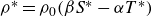 $\rho ^* = \rho _0 (\beta S^*-\alpha T^*)$
, where
$\rho ^* = \rho _0 (\beta S^*-\alpha T^*)$
, where
 $S^* = S-S_\infty$
and
$S^* = S-S_\infty$
and
 $T^* = T-T_\infty$
. Values of the local thermal expansion coefficient (
$T^* = T-T_\infty$
. Values of the local thermal expansion coefficient (
 $\alpha$
), haline contraction coefficient (
$\alpha$
), haline contraction coefficient (
 $\beta$
), kinematic viscosity (
$\beta$
), kinematic viscosity (
 $\nu$
), thermal diffusivity (
$\nu$
), thermal diffusivity (
 $\kappa _T$
) and salt diffusivity (
$\kappa _T$
) and salt diffusivity (
 $\kappa _S$
) used in the DNS are listed in table 2. For the nonlinear EoS cases, change in density (
$\kappa _S$
) used in the DNS are listed in table 2. For the nonlinear EoS cases, change in density (
 $\rho ^*$
) is evaluated using
$\rho ^*$
) is evaluated using
 $\rho ^* = \rho - \rho _\infty$
, where
$\rho ^* = \rho - \rho _\infty$
, where
 $\rho =f(T,S)$
as given in TEOS10 (McDougall & Barker Reference McDougall and Barker2011) (see figure 1
b,c) and
$\rho =f(T,S)$
as given in TEOS10 (McDougall & Barker Reference McDougall and Barker2011) (see figure 1
b,c) and
 $\rho _\infty$
is ambient water density.
$\rho _\infty$
is ambient water density.
Property values used in linear EoS DNS for different ambient water salinities and temperatures (e.g. Caldwell Reference Caldwell1974; Sharqawy, Lienhard & Zubair Reference Sharqawy, Lienhard and Zubair2010; McDougall & Barker Reference McDougall and Barker2011). The average thermal expansion coefficient
 $\alpha _a \equiv -( {\rho _\infty -\rho _i})/({\rho _0(T_\infty -T_i)})$
, representing the overall thermal anomaly within the BL, where
$\alpha _a \equiv -( {\rho _\infty -\rho _i})/({\rho _0(T_\infty -T_i)})$
, representing the overall thermal anomaly within the BL, where
 $\rho _0$
is the density of water at
$\rho _0$
is the density of water at
 $S_\infty =0$
and
$S_\infty =0$
and
 $T_\infty =0$
(
$T_\infty =0$
(
 $\rho _i=\rho _0$
for
$\rho _i=\rho _0$
for
 $S_\infty =0$
). Note that the difference between the local
$S_\infty =0$
). Note that the difference between the local
 $\alpha$
and
$\alpha$
and
 $\alpha _a$
suggests that it is not easy to define a linear EoS even at higher
$\alpha _a$
suggests that it is not easy to define a linear EoS even at higher
 $T_\infty$
.
$T_\infty$
.

A dynamic boundary condition for the ice–ocean interface is applied at the left side of the domain (
 $x=0$
). We simultaneously solve three equations ((1.1), (1.2) and (1.3)) to obtain the interface conditions such as salinity, temperature and melt rate. In the DNS, the wall-normal velocity
$x=0$
). We simultaneously solve three equations ((1.1), (1.2) and (1.3)) to obtain the interface conditions such as salinity, temperature and melt rate. In the DNS, the wall-normal velocity
 $u\vert _{x=0} = \rho _{\textit{ice}}V / \rho _{\textit{water}}$
is imposed at the ice interface as in Wells & Worster (Reference Wells and Worster2011). This ensures that the wall-normal velocity depends on the vertical direction, as does the melt rate
$u\vert _{x=0} = \rho _{\textit{ice}}V / \rho _{\textit{water}}$
is imposed at the ice interface as in Wells & Worster (Reference Wells and Worster2011). This ensures that the wall-normal velocity depends on the vertical direction, as does the melt rate
 $V$
. A no-slip boundary condition (
$V$
. A no-slip boundary condition (
 $w|_{x=0} = 0$
) has been implemented at the ice wall. The ice–water interface is presumed to be planar and maintained at
$w|_{x=0} = 0$
) has been implemented at the ice wall. The ice–water interface is presumed to be planar and maintained at
 $x=0$
. This assumption is based on a large Stefan number (
$x=0$
. This assumption is based on a large Stefan number (
 $\textit{Ste} \gg 1$
; see § 6 for the definition of
$\textit{Ste} \gg 1$
; see § 6 for the definition of
 $\textit{Ste}$
), and corroborated by stable planar interfaces observed in laboratory experiments. Although this assumption is valid for the short durations required for these solutions, caution is advised since the interface morphology could potentially evolve over time due to a positive feedback between the interface shape, flow dynamics and ablation rate (e.g. Josberger & Martin Reference Josberger and Martin1981).
$\textit{Ste}$
), and corroborated by stable planar interfaces observed in laboratory experiments. Although this assumption is valid for the short durations required for these solutions, caution is advised since the interface morphology could potentially evolve over time due to a positive feedback between the interface shape, flow dynamics and ablation rate (e.g. Josberger & Martin Reference Josberger and Martin1981).
The ‘open ocean’ side of the computational domain is treated as an open boundary, where temperature and salinity are gradually returned to their background levels,
 $T_{\infty }$
and
$T_{\infty }$
and
 $S_{\infty }$
, respectively. This adjustment occurs through a ‘sponge’ area (e.g. Gayen & Sarkar Reference Gayen and Sarkar2011) spanning
$S_{\infty }$
, respectively. This adjustment occurs through a ‘sponge’ area (e.g. Gayen & Sarkar Reference Gayen and Sarkar2011) spanning
 $0.75W \geqslant x \geqslant W$
. At the top and bottom boundaries, no-slip conditions are enforced for velocities, and no-flux conditions are applied to both temperature and salinity. Periodicity is maintained in the spanwise direction (
$0.75W \geqslant x \geqslant W$
. At the top and bottom boundaries, no-slip conditions are enforced for velocities, and no-flux conditions are applied to both temperature and salinity. Periodicity is maintained in the spanwise direction (
 $y$
). The present computational domain is similar to that of the water tank. However, the semi-infinite
$y$
). The present computational domain is similar to that of the water tank. However, the semi-infinite
 $x$
direction and periodic
$x$
direction and periodic
 $y$
direction serve to preserve mass in the domain as the ice face melts, but makes the computational domain slightly different from that of the experiments. In the experiments the upward- or downward-flowing melt-water reaches the top or bottom of the tank, and can create a recirculation. The computational domain allows turning of melt-water at the top and bottom, but avoids recirculation in the domain.
$y$
direction serve to preserve mass in the domain as the ice face melts, but makes the computational domain slightly different from that of the experiments. In the experiments the upward- or downward-flowing melt-water reaches the top or bottom of the tank, and can create a recirculation. The computational domain allows turning of melt-water at the top and bottom, but avoids recirculation in the domain.
5. Velocity and temperature distributions
In this section, averaged velocity and temperature data obtained for the six experimental cases as denoted in table 1 are presented and compared with the DNS results that employ both linear and nonlinear EoS for saline water. These results are categorised into three sets to highlight the effects of varying far-field conditions and thus are discussed separately. In § 5.1, the effects of temperature on the BL profiles are discussed using cases 1, 2, 3 and 4, which have constant ambient salinity at
 $S_\infty =0$
(freshwater), and the effect of the nonlinear EoS is exemplified using cases 1, 2 and 3. In the second set that consists of case 4 (
$S_\infty =0$
(freshwater), and the effect of the nonlinear EoS is exemplified using cases 1, 2 and 3. In the second set that consists of case 4 (
 $S_\infty =0$
) and case 5 (
$S_\infty =0$
) and case 5 (
 $S_\infty =34\,\rm g\,kg^{- 1}$
) at constant temperature (
$S_\infty =34\,\rm g\,kg^{- 1}$
) at constant temperature (
 $4^\circ \, \text{C}$
), comparisons are made in § 5.2 to understand how salinity influences the BL profiles. Finally, in § 5.3, cases 5 and 6, which also have a salinity of 34
$4^\circ \, \text{C}$
), comparisons are made in § 5.2 to understand how salinity influences the BL profiles. Finally, in § 5.3, cases 5 and 6, which also have a salinity of 34
 $\rm g\,kg^{- 1}$
but different far-field temperatures, comparisons are made with each other to study the effect of
$\rm g\,kg^{- 1}$
but different far-field temperatures, comparisons are made with each other to study the effect of
 $T_\infty$
on the saline water BL profiles. In §§ 5.1–5.3, the standard deviations of the measurements are shown in error bars for each case. These provide a measure of uncertainty in the measurements, although changes in flow velocity may also have contributed to these quantities. It can be observed that the agreement between the DNS and experiment profiles is generally slightly poorer in the outer region when compared with other regions of the profiles. This deviation of experimental results from simulation results is partly due to small recirculations occurring in the tank, caused by the finite size of the experimental domain. Furthermore, due to experimental limitations (of laser reflection and scattering from the ice face), the velocity data closest to the ice–water interface become more uncertain. Note that a nonlinear EoS DNS was not conducted for case 1, as the nonlinear effects were expected to be weak at this temperature. The values of
$T_\infty$
on the saline water BL profiles. In §§ 5.1–5.3, the standard deviations of the measurements are shown in error bars for each case. These provide a measure of uncertainty in the measurements, although changes in flow velocity may also have contributed to these quantities. It can be observed that the agreement between the DNS and experiment profiles is generally slightly poorer in the outer region when compared with other regions of the profiles. This deviation of experimental results from simulation results is partly due to small recirculations occurring in the tank, caused by the finite size of the experimental domain. Furthermore, due to experimental limitations (of laser reflection and scattering from the ice face), the velocity data closest to the ice–water interface become more uncertain. Note that a nonlinear EoS DNS was not conducted for case 1, as the nonlinear effects were expected to be weak at this temperature. The values of
 $\alpha$
and
$\alpha$
and
 $\alpha _a$
in table 2, however, suggest that even at such high temperatures, defining a linear approximation of the thermal expansion coefficient could be difficult for ice-melting calculations.
$\alpha _a$
in table 2, however, suggest that even at such high temperatures, defining a linear approximation of the thermal expansion coefficient could be difficult for ice-melting calculations.
Experimental (a) velocity and (b) temperature profiles of cases 1 ![]() (
(
 $T_\infty =20^\circ \, \text{C}$
), 2
$T_\infty =20^\circ \, \text{C}$
), 2 ![]() (
(
 $15^{\,\circ} \text{C}$
), 3
$15^{\,\circ} \text{C}$
), 3 ![]() (
(
 $10^{\,\circ} \text{C}$
) and 4
$10^{\,\circ} \text{C}$
) and 4 ![]() (
(
 $4^{\,\circ} \text{C}$
). Here solid lines represent nonlinear EoS DNS. Note that only for case 1 are linear EoS DNS data shown.
$4^{\,\circ} \text{C}$
). Here solid lines represent nonlinear EoS DNS. Note that only for case 1 are linear EoS DNS data shown.

5.1. Freshwater (
 $S_\infty =0$
) cases: effect of
$T_\infty$
and nonlinear density
$S_\infty =0$
) cases: effect of
$T_\infty$
and nonlinear density


Cases 1–4 are for freshwater. Figure 1(c) shows where these four freshwater cases lie on a T–S diagram. Cases 1, 2 and 3 (
 $T_\infty =20$
,
$T_\infty =20$
,
 $15$
and
$15$
and
 $10^{\,\circ} \text{C}$
) lie at the edge of region II (see figure 1
b) where bi-directional flows could be observed, but which is less likely for zero ambient salinity and sufficiently away from
$10^{\,\circ} \text{C}$
) lie at the edge of region II (see figure 1
b) where bi-directional flows could be observed, but which is less likely for zero ambient salinity and sufficiently away from
 $4^{\,\circ} \text{C}$
. In figure 5(a) and 5(b), respectively, velocity and temperature profiles from experiments are presented along with nonlinear EoS DNS profiles. Cases 1–3 in figure 5(a) show a uni-directional downward flow with velocity magnitude increasing with increasing far-field temperature. This increase is due to the increase in density difference between far field and interface. Case 4 shows a uni-directional upward flow. The experimental velocity and temperature data show a reasonable agreement with those of the DNS, with the differences primarily attributable to the recirculation present in the experiments and to the estimation of the virtual origin of the BL. The effects of this recirculation are most significant in case 1, where the flow velocity is highest.
$4^{\,\circ} \text{C}$
. In figure 5(a) and 5(b), respectively, velocity and temperature profiles from experiments are presented along with nonlinear EoS DNS profiles. Cases 1–3 in figure 5(a) show a uni-directional downward flow with velocity magnitude increasing with increasing far-field temperature. This increase is due to the increase in density difference between far field and interface. Case 4 shows a uni-directional upward flow. The experimental velocity and temperature data show a reasonable agreement with those of the DNS, with the differences primarily attributable to the recirculation present in the experiments and to the estimation of the virtual origin of the BL. The effects of this recirculation are most significant in case 1, where the flow velocity is highest.
The ‘flow reversal’ in case 4, where the density variation is purely from temperature, is a symptom of the nonlinear variation of water density. Here, the flow is upward because water has a density maximum at
 $4^{\,\circ} \text{C}$
and the melt-water released from the ice interface is less dense than ambient water. These flow behaviours can be understood by referencing the density variation of freshwater with temperature (see figure 1
c) and the average thermal expansion coefficient
$4^{\,\circ} \text{C}$
and the melt-water released from the ice interface is less dense than ambient water. These flow behaviours can be understood by referencing the density variation of freshwater with temperature (see figure 1
c) and the average thermal expansion coefficient
 $\alpha _a \equiv -(\rho _\infty -\rho _i)/(\rho _0(T_\infty -T_i))$
values in table 2, where
$\alpha _a \equiv -(\rho _\infty -\rho _i)/(\rho _0(T_\infty -T_i))$
values in table 2, where
 $\alpha _a$
becomes negative in case 4, indicating that the average density within the BL is lower than that of the ambient water at this ambient temperature. Since all these cases are for freshwater, one does not observe any upward inner layer, and the flow is uni-directional downward. Case 4 lies on the boundary between regions I and II. This suggests that freshwater flow reversal happens at an ambient temperature between
$\alpha _a$
becomes negative in case 4, indicating that the average density within the BL is lower than that of the ambient water at this ambient temperature. Since all these cases are for freshwater, one does not observe any upward inner layer, and the flow is uni-directional downward. Case 4 lies on the boundary between regions I and II. This suggests that freshwater flow reversal happens at an ambient temperature between
 $4$
and
$4$
and
 $10^{\,\circ} \text{C}$
, and hence line
$10^{\,\circ} \text{C}$
, and hence line
 $T_\textit{md}$
(in figure 1
b) is not the exact boundary between upward and downward flows. From figure 5(a) it is also apparent that the peak location of the velocity profiles moves slightly further from the interface and the peak velocity magnitude decreases with decreasing
$T_\textit{md}$
(in figure 1
b) is not the exact boundary between upward and downward flows. From figure 5(a) it is also apparent that the peak location of the velocity profiles moves slightly further from the interface and the peak velocity magnitude decreases with decreasing
 $T_\infty$
. Consistently, in figure 5(b) the thermal BL thickness (say,
$T_\infty$
. Consistently, in figure 5(b) the thermal BL thickness (say,
 $\delta _T$
) increases with decreasing
$\delta _T$
) increases with decreasing
 $T_\infty$
. This is a result of the decreasing heat transfer rate that reduces the temperature gradient (
$T_\infty$
. This is a result of the decreasing heat transfer rate that reduces the temperature gradient (
 $\partial T/\partial x$
) as
$\partial T/\partial x$
) as
 $T_\infty$
decreases as expected for a laminar BL. In fact, the peak vertical velocity
$T_\infty$
decreases as expected for a laminar BL. In fact, the peak vertical velocity
 $w_{\textit{max}} \sim [g\alpha (T_\infty - T_i)z]^{1/2}$
and the BL thickness
$w_{\textit{max}} \sim [g\alpha (T_\infty - T_i)z]^{1/2}$
and the BL thickness
 $\delta \sim \delta _T \sim [\nu \kappa _T z /(g \alpha (T_\infty - T_i))]^{1/4}$
, which come from the order-of-magnitude matching of viscous diffusion and buoyancy force in the vertical momentum equation,
$\delta \sim \delta _T \sim [\nu \kappa _T z /(g \alpha (T_\infty - T_i))]^{1/4}$
, which come from the order-of-magnitude matching of viscous diffusion and buoyancy force in the vertical momentum equation,
 $\nu w_{\textit{max}}/\delta ^2 \sim g \alpha (T_\infty - T_i)$
, and the vertical advection and thermal diffusion in the temperature equation,
$\nu w_{\textit{max}}/\delta ^2 \sim g \alpha (T_\infty - T_i)$
, and the vertical advection and thermal diffusion in the temperature equation,
 $w_{\textit{max}}/z \sim \kappa _T/\delta ^2$
(see also Appendix A and Ostrach Reference Ostrach1952; Kuiken Reference Kuiken1968; Josberger & Martin Reference Josberger and Martin1981; Carey & Gebhart Reference Carey and Gebhart1982b
). The data in figure 5(a) show expected trends of
$w_{\textit{max}}/z \sim \kappa _T/\delta ^2$
(see also Appendix A and Ostrach Reference Ostrach1952; Kuiken Reference Kuiken1968; Josberger & Martin Reference Josberger and Martin1981; Carey & Gebhart Reference Carey and Gebhart1982b
). The data in figure 5(a) show expected trends of
 $w_{\textit{max}}$
and
$w_{\textit{max}}$
and
 $\delta$
with
$\delta$
with
 $(T_\infty - T_i)$
. The variation with
$(T_\infty - T_i)$
. The variation with
 $z$
is discussed in the context of melt-rate scaling in § 6.
$z$
is discussed in the context of melt-rate scaling in § 6.
Comparison of experimental (symbols), DNS with linear EoS (dashed lines) and DNS with nonlinear EoS (solid lines). (a,d,g) Velocity (
 $w$
) profiles for cases 3
$w$
) profiles for cases 3 ![]() , 2
, 2 ![]() and 1
and 1 ![]() , respectively. (b,e,h) Comparison of non-dimensional experimental and DNS (linear and nonlinear EoS) velocity (
, respectively. (b,e,h) Comparison of non-dimensional experimental and DNS (linear and nonlinear EoS) velocity (
 $\tilde {w}^*\equiv (w z_1/2\nu )\textit{Gr}_{z_1}^{-1/2}$
) profiles. (c,f,i) Non-dimensional temperature (
$\tilde {w}^*\equiv (w z_1/2\nu )\textit{Gr}_{z_1}^{-1/2}$
) profiles. (c,f,i) Non-dimensional temperature (
 $\tilde {T}\equiv {(T_\infty -T)}/{( T_\infty -T_i)}$
; see Appendix A, (A2)) profiles along with the analytical solution for
$\tilde {T}\equiv {(T_\infty -T)}/{( T_\infty -T_i)}$
; see Appendix A, (A2)) profiles along with the analytical solution for
 $\textit{Pr}=10$
(black dashed lines) for cases 1, 2 and 3. The DNS results are presented for
$\textit{Pr}=10$
(black dashed lines) for cases 1, 2 and 3. The DNS results are presented for
 $z$
values of
$z$
values of
 $35$
,
$35$
,
 $55$
and
$55$
and
 $75$
mm, and the colour gets darker as
$75$
mm, and the colour gets darker as
 $z$
increases.
$z$
increases.

From figure 5, it is evident that both the velocity and temperature measurements are obtained very close to the ice–water interface (within 1 mm), and ambient velocity and temperature conditions are captured and show a reasonable agreement with DNS. Because of the higher temperature difference and limited size of the tank, in case 1, the temperature drops slightly from the specified ambient temperature over the duration of the experiments. This effect is apparent in figure 5(b).
Averaged velocity and temperature profiles obtained experimentally for cases 1, 2 and 3 are compared separately with the DNS in figure 6 to investigate the nonlinear effects further. Here, the DNS is run separately, first with a linear and then a nonlinear EoS relating temperature and salinity to density. The left-hand column of figure 6 shows dimensional vertical velocities whereas the middle and right-hand columns present non-dimensional velocity and temperature; rows top to bottom represent, in order, cases 1–3. Figure 6(a,d,g) shows a comparison between the experimental and DNS vertical velocity profiles. Note that nonlinear EoS DNS results are not shown for case 1. Here, the dashed (grey) lines are for the DNS using a linear EoS, while the nonlinear EoS results are in solid (blue) lines. The figure shows that the measured data are well within the range of velocities obtained from the DNS. We note that the precise velocity magnitudes are sensitive to the accurate choice of the
 $z$
location (virtual origin effect). As such, in figure 6 we show DNS velocity and temperature profiles at three different
$z$
location (virtual origin effect). As such, in figure 6 we show DNS velocity and temperature profiles at three different
 $z$
locations. It is well known that the BL does not start precisely at the ‘leading edge’ or the free surface, and a correction in terms of virtual origin is usually required.
$z$
locations. It is well known that the BL does not start precisely at the ‘leading edge’ or the free surface, and a correction in terms of virtual origin is usually required.
Far-field conditions and corresponding non-dimensional parameters (experimental)
 $R$
and
$R$
and
 $\varLambda$
that characterise resulting BL flow.
$\varLambda$
that characterise resulting BL flow.

Both the experimental and the DNS profiles are non-dimensionalised, and compared with the analytical similarity solution of Ostrach (Reference Ostrach1952) of the BL equations (see (A1) with
 $S=0$
) for natural convection along an isothermally cooled vertical flat plate at a fixed Prandtl number of 10 and a fixed thermal expansion coefficient (
$S=0$
) for natural convection along an isothermally cooled vertical flat plate at a fixed Prandtl number of 10 and a fixed thermal expansion coefficient (
 $\beta$
) (i.e. linear EoS) in figure 6(b), 6(e) and 6(h) for cases 1, 2 and 3, respectively. Note that Ostrach (Reference Ostrach1952) does not account for the melting on the boundary conditions that can influence the near-wall behaviour (Carey & Gebhart Reference Carey and Gebhart1982b
) and also neglects the nonlinearity of the EoS, which can affect the convergence of similarity solutions if BL flow becomes bi-directional (Gebhart & Mollendorf Reference Gebhart and Mollendorf1977; Carey & Gebhart Reference Carey and Gebhart1982a
,
Reference Carey and Gebhartb
). The present DNS, however, accounts for both the melting BL as well as the nonlinearity.
$\beta$
) (i.e. linear EoS) in figure 6(b), 6(e) and 6(h) for cases 1, 2 and 3, respectively. Note that Ostrach (Reference Ostrach1952) does not account for the melting on the boundary conditions that can influence the near-wall behaviour (Carey & Gebhart Reference Carey and Gebhart1982b
) and also neglects the nonlinearity of the EoS, which can affect the convergence of similarity solutions if BL flow becomes bi-directional (Gebhart & Mollendorf Reference Gebhart and Mollendorf1977; Carey & Gebhart Reference Carey and Gebhart1982a
,
Reference Carey and Gebhartb
). The present DNS, however, accounts for both the melting BL as well as the nonlinearity.
In these figures, the abscissa (
 $x$
) is non-dimensionalised as
$x$
) is non-dimensionalised as
 $x/l_T = (x/z_1)(\textit{Gr}_{z_1}/4)^{1/4}$
, where
$x/l_T = (x/z_1)(\textit{Gr}_{z_1}/4)^{1/4}$
, where
 $l_T := [4 \nu ^2 z_1/(g \alpha (T_\infty -T_i))]^{1/4}$
is here defined with
$l_T := [4 \nu ^2 z_1/(g \alpha (T_\infty -T_i))]^{1/4}$
is here defined with
 $z_1=H-z$
rather than
$z_1=H-z$
rather than
 $z$
(as in (A6)) since the flow is downwards starting from the top of the ice face, and the vertical velocity
$z$
(as in (A6)) since the flow is downwards starting from the top of the ice face, and the vertical velocity
 $w$
on the ordinate is normalised as
$w$
on the ordinate is normalised as
 $\tilde {w}^*\equiv w/(4z_1 \nu /l_T^2) = (w z_1/2\nu )\textit{Gr}_{z_1}^{-1/2}$
. This analytical solution is used as a reference profile to observe the changes in velocity profiles due to changing
$\tilde {w}^*\equiv w/(4z_1 \nu /l_T^2) = (w z_1/2\nu )\textit{Gr}_{z_1}^{-1/2}$
. This analytical solution is used as a reference profile to observe the changes in velocity profiles due to changing
 $T_\infty$
and the nonlinear effect of temperature on density. It can be observed that with a virtual origin shift of 28 mm, non-dimensionalised experimental velocity profiles nearly coincide with the nonlinear EoS DNS profiles.
$T_\infty$
and the nonlinear effect of temperature on density. It can be observed that with a virtual origin shift of 28 mm, non-dimensionalised experimental velocity profiles nearly coincide with the nonlinear EoS DNS profiles.
When non-dimensional peak velocities are compared across the three cases in figures 6(b), 6(e) and 6(h), the difference between peak velocities from measurements and linear analytical solution (as well as linear EoS DNS) increases with decreasing
 $T_\infty$
. As shown in table 3, the non-dimensional parameter
$T_\infty$
. As shown in table 3, the non-dimensional parameter
 $R$
(see (2.3)) also decreases with decreasing
$R$
(see (2.3)) also decreases with decreasing
 $T_\infty$
for these cases, indicating increasing nonlinear effects. This reduction of peak velocity demonstrates how the effects of nonlinearity of density variation become more significant as ambient temperature approaches the temperature corresponding to the density maximum (
$T_\infty$
for these cases, indicating increasing nonlinear effects. This reduction of peak velocity demonstrates how the effects of nonlinearity of density variation become more significant as ambient temperature approaches the temperature corresponding to the density maximum (
 $4^{\,\circ} \text{C}$
for freshwater). This is also apparent in the (
$4^{\,\circ} \text{C}$
for freshwater). This is also apparent in the (
 $\rho , T$
) diagram of figure 1(c). For the low-temperature cases, the density difference between ambient water and water released from ice melting is smaller than what the linear EoS assumes. Hence, the linear EoS overestimates the velocity magnitude. Further, it is also noticeable that the peak velocity location of the nonlinear EoS DNS velocity profiles is in better agreement with the measured profile than the linear EoS DNS results or the similarity solution. This highlights the role of the nonlinear EoS in momentum transport. These differences are, however, less apparent in the temperature BL profiles shown in figures 6(c), 6( f) and 6(i) where the experimental and DNS profiles show a closer agreement. Within the thermal BL (say at
$\rho , T$
) diagram of figure 1(c). For the low-temperature cases, the density difference between ambient water and water released from ice melting is smaller than what the linear EoS assumes. Hence, the linear EoS overestimates the velocity magnitude. Further, it is also noticeable that the peak velocity location of the nonlinear EoS DNS velocity profiles is in better agreement with the measured profile than the linear EoS DNS results or the similarity solution. This highlights the role of the nonlinear EoS in momentum transport. These differences are, however, less apparent in the temperature BL profiles shown in figures 6(c), 6( f) and 6(i) where the experimental and DNS profiles show a closer agreement. Within the thermal BL (say at
 $x/l_T \approx 1$
) in figures 6(c) and 6( f), however, careful inspection reveals that the nonlinear data (solid lines) compare more favourably with the experimental data. This further highlights the apparent importance of the nonlinear EoS in numerical simulations. Nonetheless, as mentioned before, even for case 1, the differences in
$x/l_T \approx 1$
) in figures 6(c) and 6( f), however, careful inspection reveals that the nonlinear data (solid lines) compare more favourably with the experimental data. This further highlights the apparent importance of the nonlinear EoS in numerical simulations. Nonetheless, as mentioned before, even for case 1, the differences in
 $\alpha$
and
$\alpha$
and
 $\alpha _a$
suggest that one could improve the linear approximations with a different definition of
$\alpha _a$
suggest that one could improve the linear approximations with a different definition of
 $\alpha$
.
$\alpha$
.
5.2. Effects of salinity:
$T_\infty =4$
(
$S_\infty = 0$
and
$34$
‰)


Experimental (a) velocity and (b) temperature BL profiles of case 4 ![]() :
:
 $S_\infty =0$
g kg−1,
$S_\infty =0$
g kg−1,
 $T_\infty =4^{\,\circ} \text{C}$
; and case 5
$T_\infty =4^{\,\circ} \text{C}$
; and case 5 ![]() :
:
 $S_\infty =34$
g kg−1,
$S_\infty =34$
g kg−1,
 $T_\infty =4^{\,\circ} \text{C}$
. Here solid lines represent nonlinear EoS DNS results.
$T_\infty =4^{\,\circ} \text{C}$
. Here solid lines represent nonlinear EoS DNS results.

In this section, velocity and temperature profiles obtained for cases 4 and 5 are compared to study the effects of
 $S_\infty$
. Here,
$S_\infty$
. Here,
 $T_\infty$
is held constant at
$T_\infty$
is held constant at
 $4^{\,\circ} \text{C}$
. As depicted in figure 7, after introducing a salinity of 34 ‰ to freshwater, the velocity profile and melt BL dynamics are completely altered. The combined effect of both salinity and temperature governs the density in the far field as well as within the BL, causing the apparent complex behaviour of the BL flow. Instead of the fully upward flow observed for case 4, case 5 shows a bi-directional flow where a thin inner upward flow is accompanied by a broader outer downward flow.
$4^{\,\circ} \text{C}$
. As depicted in figure 7, after introducing a salinity of 34 ‰ to freshwater, the velocity profile and melt BL dynamics are completely altered. The combined effect of both salinity and temperature governs the density in the far field as well as within the BL, causing the apparent complex behaviour of the BL flow. Instead of the fully upward flow observed for case 4, case 5 shows a bi-directional flow where a thin inner upward flow is accompanied by a broader outer downward flow.
To understand the combined effect of temperature and salinity that drives this BL, the DNS velocity profile for case 5 of figure 7(a) is re-plotted in figure 8(a); the corresponding density difference (
 $\Delta \rho = \rho _\infty - \rho$
) is presented in figure 8(b); and the salinity–temperature profile is plotted in figure 8(c). In all these profiles, points are marked at different distances from the interface and increasing marker size represents the increasing distance from the ice face. When the segment between the first and third markers from the interface in the velocity profile is considered, flow is predominantly upward close to the interface. This is apparent from the density profile in figure 8(b), where
$\Delta \rho = \rho _\infty - \rho$
) is presented in figure 8(b); and the salinity–temperature profile is plotted in figure 8(c). In all these profiles, points are marked at different distances from the interface and increasing marker size represents the increasing distance from the ice face. When the segment between the first and third markers from the interface in the velocity profile is considered, flow is predominantly upward close to the interface. This is apparent from the density profile in figure 8(b), where
 $\Delta \rho$
increases markedly as the wall is approached. When the same region is considered in the T–S diagram (figure 8
c), it is clear that this density change is principally due to the variation of salinity within that region. Although temperature changes slightly within that segment, its contribution to density change is negligible compared with salinity variation, as the density contours are mostly vertical in this region of the T–S diagram. Since the density close to the interface is smaller than that in the far field, an inner upward flow is observed within this segment. The flow is, however, mainly downward between the third and last markers. The reason for this is not obvious in the
$\Delta \rho$
increases markedly as the wall is approached. When the same region is considered in the T–S diagram (figure 8
c), it is clear that this density change is principally due to the variation of salinity within that region. Although temperature changes slightly within that segment, its contribution to density change is negligible compared with salinity variation, as the density contours are mostly vertical in this region of the T–S diagram. Since the density close to the interface is smaller than that in the far field, an inner upward flow is observed within this segment. The flow is, however, mainly downward between the third and last markers. The reason for this is not obvious in the
 $\Delta \rho$
profile in figure 8(b) as the density variation is quite small owing to negligible salinity change in this region (outside the salt BL). If, however, this segment of the profile is enlarged, the T–S diagram (in figure 8
c) shows that the slightly curved density contours within this region induce a density increase due to decreasing temperature. Note that at
$\Delta \rho$
profile in figure 8(b) as the density variation is quite small owing to negligible salinity change in this region (outside the salt BL). If, however, this segment of the profile is enlarged, the T–S diagram (in figure 8
c) shows that the slightly curved density contours within this region induce a density increase due to decreasing temperature. Note that at
 $S_\infty =34$
‰, the density monotonically decreases with increasing temperature. This is unlike the freshwater case where
$S_\infty =34$
‰, the density monotonically decreases with increasing temperature. This is unlike the freshwater case where
 $\rho$
peaks at
$\rho$
peaks at
 ${\approx} 4^{\,\circ} \text{C}$
. Although this density variation is quite small compared with the density variation due to salinity, it is present over a broader region and, as described in § 2.2, this leads to a downward outer flow.
${\approx} 4^{\,\circ} \text{C}$
. Although this density variation is quite small compared with the density variation due to salinity, it is present over a broader region and, as described in § 2.2, this leads to a downward outer flow.
(a) Velocity (
 $w$
) and (b)
$w$
) and (b)
 $\Delta \rho = \rho _\infty -\rho$
from nonlinear DNS for case 5. Blue and red dashed lines represent, respectively,
$\Delta \rho = \rho _\infty -\rho$
from nonlinear DNS for case 5. Blue and red dashed lines represent, respectively,
 $\beta \rho _0(S_\infty -S)$
and
$\beta \rho _0(S_\infty -S)$
and
 $10\,\alpha \rho _0(T_\infty -T)$
. Here, the value of
$10\,\alpha \rho _0(T_\infty -T)$
. Here, the value of
 $\alpha \rho _0(T_\infty -T)$
is multiplied by a factor 10 for visualisation only. (c) Temperature–salinity curve of case 5 plotted on a T–S diagram with contours denoting the water density. In all these profiles, points are marked at different distances from the interface and increasing marker size represents increasing distance from the ice face.
$\alpha \rho _0(T_\infty -T)$
is multiplied by a factor 10 for visualisation only. (c) Temperature–salinity curve of case 5 plotted on a T–S diagram with contours denoting the water density. In all these profiles, points are marked at different distances from the interface and increasing marker size represents increasing distance from the ice face.

Note that within the salinity BL (between the first and third markers from the interface), density changes by roughly 16
 $\textrm {kg}\,\textrm {m}^{- 3}$
while within the rest of the BL where the downward flow can be observed, the density change is much smaller than 1
$\textrm {kg}\,\textrm {m}^{- 3}$
while within the rest of the BL where the downward flow can be observed, the density change is much smaller than 1
 $\textrm {kg}\,\textrm {m}^{- 3}$
. The density difference contributions of salinity and temperature,
$\textrm {kg}\,\textrm {m}^{- 3}$
. The density difference contributions of salinity and temperature,
 $\beta \rho _0(S_\infty -S)$
and
$\beta \rho _0(S_\infty -S)$
and
 $\alpha \rho _0(T_\infty -T)$
, are shown in figure 8(b). The value of
$\alpha \rho _0(T_\infty -T)$
, are shown in figure 8(b). The value of
 $\alpha \rho _0(T_\infty -T)$
is multiplied by a factor 10 for visualisation, suggesting that
$\alpha \rho _0(T_\infty -T)$
is multiplied by a factor 10 for visualisation, suggesting that
 $\alpha \rho _0(T_\infty -T)$
values are small, i.e.
$\alpha \rho _0(T_\infty -T)$
values are small, i.e.
 $\Delta \rho _S$
 $ \gg \Delta \rho _T$
, resulting in
$ \gg \Delta \rho _T$
, resulting in
 ${\varLambda }\ll 1$
(see (2.2)). Interestingly, the much weaker thermal buoyancy (
${\varLambda }\ll 1$
(see (2.2)). Interestingly, the much weaker thermal buoyancy (
 $\Delta \rho _T$
) gives rise to a downward flow with comparable (if not larger) velocity magnitude and much larger mass flow rate. Conversely, the inner upward flow is driven by a much larger salinity buoyancy
$\Delta \rho _T$
) gives rise to a downward flow with comparable (if not larger) velocity magnitude and much larger mass flow rate. Conversely, the inner upward flow is driven by a much larger salinity buoyancy
 $\Delta \rho _S$
as shown in figure 7(a). As discussed in § 2.2, the reason for this difference is the relative thickness of thermal and salinity BLs (
$\Delta \rho _S$
as shown in figure 7(a). As discussed in § 2.2, the reason for this difference is the relative thickness of thermal and salinity BLs (
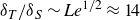 $\delta _T/\delta _S \sim \textit{Le}^{1/2}\approx 14$
) and the magnitude of the relative total buoyancy force (
$\delta _T/\delta _S \sim \textit{Le}^{1/2}\approx 14$
) and the magnitude of the relative total buoyancy force (
 ${\varLambda } \textit{Le}^{1/2}$
) acting on each of these BLs. Experimental
${\varLambda } \textit{Le}^{1/2}$
) acting on each of these BLs. Experimental
 $\varLambda$
and
$\varLambda$
and
 ${\varLambda } \textit{Le}^{1/2}$
values for cases 5 and 6 are presented in table 3 and their positions on the
${\varLambda } \textit{Le}^{1/2}$
values for cases 5 and 6 are presented in table 3 and their positions on the
 ${\varLambda }{-}\textit{Le}$
diagram are shown in figure 2 using dashed (blue and red) lines. This figure shows that, in case 5, although
${\varLambda }{-}\textit{Le}$
diagram are shown in figure 2 using dashed (blue and red) lines. This figure shows that, in case 5, although
 $\varLambda$
is small (
$\varLambda$
is small (
 $0.026$
),
$0.026$
),
 ${\varLambda } \textit{Le}^{1/2}$
is an order of magnitude larger (
${\varLambda } \textit{Le}^{1/2}$
is an order of magnitude larger (
 ${\approx}0.29$
) because of larger thermal diffusivity relative to that of salt. This indicates the significance of the relative thickness of thermal and salinity BLs (
${\approx}0.29$
) because of larger thermal diffusivity relative to that of salt. This indicates the significance of the relative thickness of thermal and salinity BLs (
 $\textit{Le}^{1/2}$
) on the buoyancy force. Even relative buoyancy force does not fully explain this flow behaviour as
$\textit{Le}^{1/2}$
) on the buoyancy force. Even relative buoyancy force does not fully explain this flow behaviour as
 ${\varLambda } \textit{Le}^{1/2}=0.29\lt 1$
indicates the presence of an overall larger salt buoyancy force within the BL. The appropriate explanation is that even though the salinity buoyancy force – driving the upward flow – is larger in magnitude, it is confined closer to the wall. Conversely, the buoyancy force from temperature – driving the downward flow – is well outside the effects of the salinity BL and the wall shear stress. Also, the salinity BL flow, owing to its proximity to the no-slip wall, is affected more compared with the thermal BL that is farther from the wall.
${\varLambda } \textit{Le}^{1/2}=0.29\lt 1$
indicates the presence of an overall larger salt buoyancy force within the BL. The appropriate explanation is that even though the salinity buoyancy force – driving the upward flow – is larger in magnitude, it is confined closer to the wall. Conversely, the buoyancy force from temperature – driving the downward flow – is well outside the effects of the salinity BL and the wall shear stress. Also, the salinity BL flow, owing to its proximity to the no-slip wall, is affected more compared with the thermal BL that is farther from the wall.
Experimental (a) velocity and (b) temperature BL profiles of case 5 ![]() :
:
 $S_\infty =34$
g kg−1,
$S_\infty =34$
g kg−1,
 $T_\infty =4^{\,\circ} \text{C}$
; and case 6
$T_\infty =4^{\,\circ} \text{C}$
; and case 6 ![]() :
:
 $S_\infty =34$
g kg−1,
$S_\infty =34$
g kg−1,
 $T_\infty =2^{\,\circ} \text{C}$
. Here solid lines represent nonlinear EoS DNS results.
$T_\infty =2^{\,\circ} \text{C}$
. Here solid lines represent nonlinear EoS DNS results.

Figure 7 shows that the experiments capture well the features of the complex bi-directional BL flow, and is in agreement with the nonlinear DNS. Another important fact that needs to be highlighted here is the freezing point depression due to the salinity in the temperature profile in figure 7(b). In case 5, the measured interface temperature is approximately 1 degree below
 $0^{\,\circ} \text{C}$
, matching with the interface temperature estimated in the DNS. Note that this interface temperature (
$0^{\,\circ} \text{C}$
, matching with the interface temperature estimated in the DNS. Note that this interface temperature (
 $T_i$
) also allows one to calculate the interface salinity:
$T_i$
) also allows one to calculate the interface salinity:
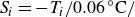 $S_i=-T_i/{0.06}^{\,\circ} \text{C}/$
‰
$S_i=-T_i/{0.06}^{\,\circ} \text{C}/$
‰
 $ \approx 16.7$
g kg−1.
$ \approx 16.7$
g kg−1.
5.3. Effects of temperature at fixed
$S_\infty =34$
‰ (
$T_\infty =4$
and
$2^{\,\circ} \text{C}$
)


For a fixed
 $S_\infty =34$
‰, case 5 (
$S_\infty =34$
‰, case 5 (
 $T_\infty =4^{\,\circ} \text{C}$
) and case 6 (
$T_\infty =4^{\,\circ} \text{C}$
) and case 6 (
 $T_\infty =2^{\,\circ} \text{C}$
) are compared to study the effect of temperature in saline water. For these cases, figure 9(a) displays vertical velocities and figure 9(b) temperatures. In case 5 the downward peak velocity magnitude is slightly larger than in case 6. This is owing to the larger
$T_\infty =2^{\,\circ} \text{C}$
) are compared to study the effect of temperature in saline water. For these cases, figure 9(a) displays vertical velocities and figure 9(b) temperatures. In case 5 the downward peak velocity magnitude is slightly larger than in case 6. This is owing to the larger
 $\Delta \rho _T$
in case 5. Furthermore, the downward velocity peak is closer to the interface in case 5 compared to case 6. This is similar to the uni-directional flow in § 5.1, where thermal BL thickness decreases with increasing
$\Delta \rho _T$
in case 5. Furthermore, the downward velocity peak is closer to the interface in case 5 compared to case 6. This is similar to the uni-directional flow in § 5.1, where thermal BL thickness decreases with increasing
 $T_\infty$
, and hence the temperature effect is more pronounced closer to the interface for case 5 compared with case 6. Another interesting observation is that the interface temperature
$T_\infty$
, and hence the temperature effect is more pronounced closer to the interface for case 5 compared with case 6. Another interesting observation is that the interface temperature
 $T_i$
for case 5 is higher than that for case 6 according to figure 9(b), showing less freezing point depression for the higher-ambient-temperature case (case 5). Therefore, according to
$T_i$
for case 5 is higher than that for case 6 according to figure 9(b), showing less freezing point depression for the higher-ambient-temperature case (case 5). Therefore, according to
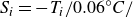 $S_i= -T_i/{0.06}^\circ C/$
‰, the interface salinity (
$S_i= -T_i/{0.06}^\circ C/$
‰, the interface salinity (
 $S_i$
) in case 5 should be less than in case 6. The reduction in
$S_i$
) in case 5 should be less than in case 6. The reduction in
 $T_i$
as
$T_i$
as
 $T_\infty$
decreases can be calculated from the quadratic equation (2.6) as shown in figure 2(c). These calculations show that for
$T_\infty$
decreases can be calculated from the quadratic equation (2.6) as shown in figure 2(c). These calculations show that for
 $T_\infty =4$
and
$T_\infty =4$
and
 $2^{\,\circ} \text{C}$
the corresponding
$2^{\,\circ} \text{C}$
the corresponding
 $T_i\approx -1$
and
$T_i\approx -1$
and
 $-1.4^{\,\circ} \text{C}$
, which are in reasonable agreement with the experimental and DNS data presented in figure 9(b). Reduction of interface salinity in case 5 increases
$-1.4^{\,\circ} \text{C}$
, which are in reasonable agreement with the experimental and DNS data presented in figure 9(b). Reduction of interface salinity in case 5 increases
 $\Delta \rho _S$
. This increased
$\Delta \rho _S$
. This increased
 $\Delta \rho _s$
results in a slight velocity increase in the inner upward flow as shown in figure 9(a). This feature is more clearly observed in the DNS, although it is difficult to discern in the experimental data.
$\Delta \rho _s$
results in a slight velocity increase in the inner upward flow as shown in figure 9(a). This feature is more clearly observed in the DNS, although it is difficult to discern in the experimental data.
The experimental cases 5 and 6 are also presented on the
 $({\varLambda},\,\textit{Le})$
plane in figure 2(a) and 2(b). The figure also shows analytical results using (2.6) for
$({\varLambda},\,\textit{Le})$
plane in figure 2(a) and 2(b). The figure also shows analytical results using (2.6) for
 $T_\infty$
in the range of
$T_\infty$
in the range of
 $4^{\,\circ} \text{C}$
to
$4^{\,\circ} \text{C}$
to
 $-2^{\,\circ} \text{C}$
. The analytical results match experiments/DNS reasonably well, providing confidence that (2.6) can be used to calculate
$-2^{\,\circ} \text{C}$
. The analytical results match experiments/DNS reasonably well, providing confidence that (2.6) can be used to calculate
 $T_i$
, and hence the location of the flow regime on the
$T_i$
, and hence the location of the flow regime on the
 $({\varLambda },\,\textit{Le})$
plane.
$({\varLambda },\,\textit{Le})$
plane.
Ice melt rate profiles for case 1:
 $(T_\infty ,\,S_\infty )$
= (
$(T_\infty ,\,S_\infty )$
= (
 $20^{\,\circ} \text{C}$
, 0 ‰) in green; case 2: (
$20^{\,\circ} \text{C}$
, 0 ‰) in green; case 2: (
 $15^{\,\circ} \text{C}$
, 0 ‰) in yellow; case 3: (
$15^{\,\circ} \text{C}$
, 0 ‰) in yellow; case 3: (
 $10^{\,\circ} \text{C}$
, 0 ‰) in red; case 4: (
$10^{\,\circ} \text{C}$
, 0 ‰) in red; case 4: (
 $4^{\,\circ} \text{C}$
, 0 ‰) in blue; case 5: (
$4^{\,\circ} \text{C}$
, 0 ‰) in blue; case 5: (
 $4^{\,\circ} \text{C}$
, 34 ‰) in purple; and case 6: (
$4^{\,\circ} \text{C}$
, 34 ‰) in purple; and case 6: (
 $2^{\,\circ} \text{C}$
, 34 ‰) in grey. Symbols: molecular tagging images
$2^{\,\circ} \text{C}$
, 34 ‰) in grey. Symbols: molecular tagging images
 $\square$
, direct imaging
$\square$
, direct imaging
 $\triangledown$
and using (1.1) with MTT data
$\triangledown$
and using (1.1) with MTT data
 $\circ$
. Here, error bars represent the uncertainty of each measurement. The DNS with linear EoS in dashed lines and nonlinear EoS in solid lines. (a) Linear–linear plot. (b) Log–log plot, where for cases 1, 2 and 3:
$\circ$
. Here, error bars represent the uncertainty of each measurement. The DNS with linear EoS in dashed lines and nonlinear EoS in solid lines. (a) Linear–linear plot. (b) Log–log plot, where for cases 1, 2 and 3:
 $z_1=H-z$
; for cases 4, 5 and 6:
$z_1=H-z$
; for cases 4, 5 and 6:
 $z_1=z$
.
$z_1=z$
.

6. Melt rates
During the experiments, ice-face melting (or dissolution) attains a quasi-steady state. Experimental measurements of melt rates (
 $V$
) are obtained via three different methods: (i) imaging the interface directly as a function of time; (ii) by molecular tagging images (obtained during the process of MTV/MTT) that include the ice–water interface as a function of time; and (iii) employing (1.1) that uses temperature (gradient) measured within the BL from MTT. Water and ice properties used in method (iii) for applying (1.1) are:
$V$
) are obtained via three different methods: (i) imaging the interface directly as a function of time; (ii) by molecular tagging images (obtained during the process of MTV/MTT) that include the ice–water interface as a function of time; and (iii) employing (1.1) that uses temperature (gradient) measured within the BL from MTT. Water and ice properties used in method (iii) for applying (1.1) are:
 $c_w =4218.9$
 $\rm J\,kg^{- 1}\,K^{-1}$
,
$\rm J\,kg^{- 1}\,K^{-1}$
,
 $L=$
$L=$
 $333.41\times 10^{3}$
 $\rm J\,kg^{- 1}$
,
$\rm J\,kg^{- 1}$
,
 $\rho _w=$
 $999.9$
 $\textrm {kg}\,\textrm {m}^{- 3}$
and
$\textrm {kg}\,\textrm {m}^{- 3}$
and
 $\rho _{\textit{ice}} =$
 $916.7$
 $\textrm {kg}\,\textrm {m}^{- 3}$
(McDougall & Barker Reference McDougall and Barker2011). The first two methods are also described in § 3.5 with further details in Appendix E.
$\textrm {kg}\,\textrm {m}^{- 3}$
(McDougall & Barker Reference McDougall and Barker2011). The first two methods are also described in § 3.5 with further details in Appendix E.
Figure 10(a) shows ice melt rates (
 $V$
) measured experimentally using the different methods (in symbols) and from DNS (in lines) for all six cases. Both experiments and DNS results show reasonable agreement. The slight discrepancies in the melt rates between experiments and DNS under the same ambient conditions, as shown in figure 10, arise from the measurement uncertainties (indicated with error bars) as well as the inability of DNS to exactly replicate the experimental set-up and conditions. In low-temperature experiments, the effects of these uncertainties become more significant due to the low melt rates. Considering the small
$V$
) measured experimentally using the different methods (in symbols) and from DNS (in lines) for all six cases. Both experiments and DNS results show reasonable agreement. The slight discrepancies in the melt rates between experiments and DNS under the same ambient conditions, as shown in figure 10, arise from the measurement uncertainties (indicated with error bars) as well as the inability of DNS to exactly replicate the experimental set-up and conditions. In low-temperature experiments, the effects of these uncertainties become more significant due to the low melt rates. Considering the small
 $V$
values, melt rates obtained by molecular tagging and other experimental methods also exhibit reasonable agreement; however, method (i) using interface imaging seems less reliable owing to the difficulty in precisely locating the interface (see also Appendix E). Note that for case 1 the linear approximation with
$V$
values, melt rates obtained by molecular tagging and other experimental methods also exhibit reasonable agreement; however, method (i) using interface imaging seems less reliable owing to the difficulty in precisely locating the interface (see also Appendix E). Note that for case 1 the linear approximation with
 $\alpha$
could be less appropriate, and a different definition along the lines of
$\alpha$
could be less appropriate, and a different definition along the lines of
 $\alpha _a$
could produce melt rates closer to the experimental values. Furthermore, as a reference, it should be noted that observations of actual Antarctic ice shelves indicate that melt rates usually range between 0.46 and 14.6
$\alpha _a$
could produce melt rates closer to the experimental values. Furthermore, as a reference, it should be noted that observations of actual Antarctic ice shelves indicate that melt rates usually range between 0.46 and 14.6
 $\rm m\,year^{-1}$
(e.g. Rosevear, Galton-Fenzi & Stevens Reference Rosevear, Galton-Fenzi and Stevens2022). The main reason that these values are lower than experimental and DNS values (upper axis of figure 10
a) is that the ocean water temperature at Antarctic ice shelves is much closer to the freezing point. In addition to temperature differences, several other factors can also contribute to the lower melt rates observed in the Antarctic environment. These include geometric differences between the experimental configuration (vertical flat ice faces) and the natural ice shelf morphology (typically sloping ice shelves), as well as the scale and state of the BL flow. In the field, BLs are generally turbulent and have evolved over many metres or even kilometres, in contrast to the centimetre-scale laminar flow examined in the present experiments. In figure 10(a) the melt rates increase with both increasing ambient water temperature and salinity in both the measurements and the DNS. For uni-directional downward BL flows (cases 1, 2 and 3 with
$\rm m\,year^{-1}$
(e.g. Rosevear, Galton-Fenzi & Stevens Reference Rosevear, Galton-Fenzi and Stevens2022). The main reason that these values are lower than experimental and DNS values (upper axis of figure 10
a) is that the ocean water temperature at Antarctic ice shelves is much closer to the freezing point. In addition to temperature differences, several other factors can also contribute to the lower melt rates observed in the Antarctic environment. These include geometric differences between the experimental configuration (vertical flat ice faces) and the natural ice shelf morphology (typically sloping ice shelves), as well as the scale and state of the BL flow. In the field, BLs are generally turbulent and have evolved over many metres or even kilometres, in contrast to the centimetre-scale laminar flow examined in the present experiments. In figure 10(a) the melt rates increase with both increasing ambient water temperature and salinity in both the measurements and the DNS. For uni-directional downward BL flows (cases 1, 2 and 3 with
 $T_\infty =20$
,
$T_\infty =20$
,
 $15$
and
$15$
and
 $10^{\,\circ} \text{C}$
at zero salinity),
$10^{\,\circ} \text{C}$
at zero salinity),
 $V$
increases with increasing
$V$
increases with increasing
 $z$
, whereas it decreases slightly with increasing
$z$
, whereas it decreases slightly with increasing
 $z$
for uni-directional upward flow (case 4,
$z$
for uni-directional upward flow (case 4,
 $T_\infty =$
 $4^{\,\circ} \text{C}$
at zero salinity). For both bi-directional flows (cases 5 and 6, with
$4^{\,\circ} \text{C}$
at zero salinity). For both bi-directional flows (cases 5 and 6, with
 $T_\infty =4$
and
$T_\infty =4$
and
 $2^{\,\circ} \text{C}$
at
$2^{\,\circ} \text{C}$
at
 $S_\infty = 34$
‰),
$S_\infty = 34$
‰),
 $V$
is a more complicated function of
$V$
is a more complicated function of
 $z$
. The same data as in figure 10(a) are shown on a log–log scale in figure 10(b), but now as a function of
$z$
. The same data as in figure 10(a) are shown on a log–log scale in figure 10(b), but now as a function of
 $z_1 = H-z$
for cases 1, 2 and 3 because the flow is downward, whereas
$z_1 = H-z$
for cases 1, 2 and 3 because the flow is downward, whereas
 $z_1=z$
for cases 4, 5 and 6 where the flow adjacent to the ice face is upward.
$z_1=z$
for cases 4, 5 and 6 where the flow adjacent to the ice face is upward.
Before discussing the
 $z$
variation, we first focus on the relative magnitudes of
$z$
variation, we first focus on the relative magnitudes of
 $V$
for the six cases corresponding to different (
$V$
for the six cases corresponding to different (
 $T_\infty ,\, S_\infty$
). The trends of changing
$T_\infty ,\, S_\infty$
). The trends of changing
 $V$
with
$V$
with
 $T_\infty$
and
$T_\infty$
and
 $S_\infty$
are consistent with (1.1), where the ablation velocity
$S_\infty$
are consistent with (1.1), where the ablation velocity
 $V$
is directly proportional to
$V$
is directly proportional to
 $\partial T/ \partial x$
at the interface. Figures 5(b), 7(b) and 9(b) show the temperature profiles corresponding to the six cases. These reveal that the temperature gradient at the interface (
$\partial T/ \partial x$
at the interface. Figures 5(b), 7(b) and 9(b) show the temperature profiles corresponding to the six cases. These reveal that the temperature gradient at the interface (
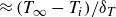 $\approx (T_\infty -T_i)/\delta _T$
) is higher for the high-
$\approx (T_\infty -T_i)/\delta _T$
) is higher for the high-
 $T_\infty$
cases compared with the lower-
$T_\infty$
cases compared with the lower-
 $T_\infty$
cases. This stem from a higher temperature difference between the interface and ambient water and a thinner thermal BL (
$T_\infty$
cases. This stem from a higher temperature difference between the interface and ambient water and a thinner thermal BL (
 $\delta _T$
). Therefore, ice melting is more vigorous in high-temperature cases compared with low-temperature cases. Furthermore, due to freezing point depression (described by
$\delta _T$
). Therefore, ice melting is more vigorous in high-temperature cases compared with low-temperature cases. Furthermore, due to freezing point depression (described by
 $T_i=-{0.06}^{\,\circ} \text{C}$
‰−1
$T_i=-{0.06}^{\,\circ} \text{C}$
‰−1
 $ \,S_i$
), ice melts at lower temperatures (below
$ \,S_i$
), ice melts at lower temperatures (below
 $0^{\,\circ} \text{C}$
) as the water salinity increases. As a result, the temperature difference between the interface and ambient water (
$0^{\,\circ} \text{C}$
) as the water salinity increases. As a result, the temperature difference between the interface and ambient water (
 $T_\infty -T_i$
) increases and consequently the temperature gradient increases at the interface. This is apparent when the temperature profiles of case 4 are compared with those of case 5 (figure 7
b), noting that both have the same
$T_\infty -T_i$
) increases and consequently the temperature gradient increases at the interface. This is apparent when the temperature profiles of case 4 are compared with those of case 5 (figure 7
b), noting that both have the same
 $T_\infty =4^{\,\circ} \text{C}$
. Therefore, the case 5 melt rate is larger than that of case 4 in figure 10.
$T_\infty =4^{\,\circ} \text{C}$
. Therefore, the case 5 melt rate is larger than that of case 4 in figure 10.
Variation of
 $V$
with
$V$
with
 $z$
is better observed in figure 10(b), where the top and bottom
$z$
is better observed in figure 10(b), where the top and bottom
 $z$
locations have been left out. These are the locations where the flow turns due to the free surface and wall, respectively. For uni-directional flow cases 1, 2, 3 (downward) and 4 (upward),
$z$
locations have been left out. These are the locations where the flow turns due to the free surface and wall, respectively. For uni-directional flow cases 1, 2, 3 (downward) and 4 (upward),
 $V$
has a clear (and expected, see below) power-law dependence:
$V$
has a clear (and expected, see below) power-law dependence:
 $V\sim z_1^{-1/4}$
. The black solid line in figure 10(b) shows the expected slope. The
$V\sim z_1^{-1/4}$
. The black solid line in figure 10(b) shows the expected slope. The
 $z_1^{-1/4}$
law can be obtained by combining the balance of viscous–buoyancy terms in the vertical momentum equation and advection–diffusion term in the temperature equation (see (A1b
) and (A1c
) in Appendix A) and the temperature flux at the interface (1.1) (e.g. Ostrach Reference Ostrach1952; Kuiken Reference Kuiken1968; Josberger & Martin Reference Josberger and Martin1981; Carey & Gebhart Reference Carey and Gebhart1982b
; Wells & Worster Reference Wells and Worster2011; Mondal et al. Reference Mondal, Gayen, Griffiths and Kerr2019). Those are, respectively,
$z_1^{-1/4}$
law can be obtained by combining the balance of viscous–buoyancy terms in the vertical momentum equation and advection–diffusion term in the temperature equation (see (A1b
) and (A1c
) in Appendix A) and the temperature flux at the interface (1.1) (e.g. Ostrach Reference Ostrach1952; Kuiken Reference Kuiken1968; Josberger & Martin Reference Josberger and Martin1981; Carey & Gebhart Reference Carey and Gebhart1982b
; Wells & Worster Reference Wells and Worster2011; Mondal et al. Reference Mondal, Gayen, Griffiths and Kerr2019). Those are, respectively,
 \begin{equation} \nu \frac {W}{\delta _T^2} \sim g\alpha (T_\infty -T_i),\quad \frac {W}{z_1} \sim \frac {\kappa _T}{\delta _T^2} \quad\textrm {and}\quad V \sim \left (\frac {\rho \,c_w}{L \,\rho _{\textit{ice}}} \right )\frac {\kappa _T (T_\infty -T_i)}{\delta _T}, \end{equation}
where
 $W$
is the magnitude of the vertical velocity and for concreteness we take
$W$
is the magnitude of the vertical velocity and for concreteness we take
 $W$
as the maximum
$W$
as the maximum
 $w$
within the BL,
$w$
within the BL,
 $w_{\textit{max}}$
. Also,
$w_{\textit{max}}$
. Also,
 $\delta _T$
(or later
$\delta _T$
(or later
 $\delta _S$
) is obtained as the
$\delta _S$
) is obtained as the
 $x$
location where
$x$
location where
 $T$
(or
$T$
(or
 $S$
) reaches
$S$
) reaches
 $0.99T_\infty$
(or
$0.99T_\infty$
(or
 $0.99S_\infty$
). Eliminating
$0.99S_\infty$
). Eliminating
 $\delta _T$
or
$\delta _T$
or
 $W$
from the first two equations in (6.1) leads to
$W$
from the first two equations in (6.1) leads to
 \begin{align} W \sim \left (\frac {g_T \kappa _T}{\nu } \right )^{1/2} z_1^{1/2} ,\quad \delta _T \sim \left (\frac {\nu \kappa _T}{g_T} \right )^{1/4} z_1^{1/4}\quad\textrm {and}\quad V \sim \left (Ste \right )^{-1}\left (\frac {\kappa _T^3 g_T }{\nu } \right )^{1/4} z_1^{-1/4}, \end{align}
where the Stefan number
 $\textit{Ste} \equiv (L \,\rho _{\textit{ice}})/(\rho \,C_p(T_\infty -T_i))$
and
$\textit{Ste} \equiv (L \,\rho _{\textit{ice}})/(\rho \,C_p(T_\infty -T_i))$
and
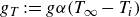 $g_T := g \alpha (T_\infty -T_i)$
. In non-dimensional form:
$g_T := g \alpha (T_\infty -T_i)$
. In non-dimensional form:
 \begin{equation} \frac {V}{W} \sim \left (\textit{Ste} \right )^{-1} \left (\textit{Gr}_H \right )^{-1/4} \left (\textit{Pr} \right )^{-1/4} \left ( \frac {z_1}{H}\right )^{-3/4}\!. \end{equation}
Hence, uni-directional flows should follow
 $V\sim z_1^{-1/4}$
as suggested by (6.2), and they do, as the data in figure 10(b) show.
$V\sim z_1^{-1/4}$
as suggested by (6.2), and they do, as the data in figure 10(b) show.
With the addition of salt (cases 5 and 6), a similar scaling is expected. Now, however, the upward flow close to the ice face is driven by the buoyancy provided by the freshwater release. If we assume salinity-driven dissolution using (1.2) as the dominant feature, i.e. the buoyancy force is dominated by salinity giving uni-directional flow, and hence
 $V \sim (\rho \kappa _S(S_\infty -S_i))/(\rho _{\textit{ice}}S_i\delta _s)$
, then instead of (6.2) we obtain (Mondal et al. Reference Mondal, Gayen, Griffiths and Kerr2019)
$V \sim (\rho \kappa _S(S_\infty -S_i))/(\rho _{\textit{ice}}S_i\delta _s)$
, then instead of (6.2) we obtain (Mondal et al. Reference Mondal, Gayen, Griffiths and Kerr2019)
 \begin{align} W \sim \left (\frac {g_S \kappa _S}{\nu } \right )^{1/2} z_1^{1/2} ,\quad \delta _S \sim \left (\frac {\nu \kappa _S}{g_S} \right )^{1/4} z_1^{1/4}\quad\textrm {and}\quad V \sim \left (\frac {\rho (S_\infty -S_i)}{\rho _{\textit{ice}}S_i} \right ) \left (\frac {\kappa _S^3 g_S }{\nu } \right )^{1/4} z_1^{-1/4}, \end{align}
where the reduced gravity due to salinity is
 $g_S := g \beta (S_\infty -S_i)$
. It is clear from figure 10(b) that the two bi-directional cases 5 and 6 do not follow the scaling
$g_S := g \beta (S_\infty -S_i)$
. It is clear from figure 10(b) that the two bi-directional cases 5 and 6 do not follow the scaling
 $V\sim z_1^{-1/4}$
expected from (6.4). Recall, however, that even for salinity-driven flows,
$V\sim z_1^{-1/4}$
expected from (6.4). Recall, however, that even for salinity-driven flows,
 $V$
is constrained to follow (1.1), where
$V$
is constrained to follow (1.1), where
 $\partial T/\partial x$
at the wall appears. Thus, apart from equations leading to (6.4),
$\partial T/\partial x$
at the wall appears. Thus, apart from equations leading to (6.4),
 $V$
also depends non-trivially on the thermal BL properties.
$V$
also depends non-trivially on the thermal BL properties.
To further clarify, two prototypical cases of uni- and bi-directional flows are considered: case 3 (
 $10^{\,\circ} \text{C}$
, 0 ‰) and case 6 (
$10^{\,\circ} \text{C}$
, 0 ‰) and case 6 (
 $2^{\,\circ} \text{C}$
, 34 ‰). The expected scalings of case 3 for
$2^{\,\circ} \text{C}$
, 34 ‰). The expected scalings of case 3 for
 $w_{\textit{max}}\sim z_1^{1/2}$
and
$w_{\textit{max}}\sim z_1^{1/2}$
and
 $\delta _T\sim z_1^{1/4}$
in (6.2) are observed from the data shown by the red lines in figures 11(a) and 11(b). Hence, for constant property (a good approximation here), the
$\delta _T\sim z_1^{1/4}$
in (6.2) are observed from the data shown by the red lines in figures 11(a) and 11(b). Hence, for constant property (a good approximation here), the
 $V\sim z_1^{-1/4}$
scaling should follow if
$V\sim z_1^{-1/4}$
scaling should follow if
 $T_i$
remains constant, as evident from (6.1). Without salinity in case 3,
$T_i$
remains constant, as evident from (6.1). Without salinity in case 3,
 $T_i=0$
, and the expected
$T_i=0$
, and the expected
 $V$
scaling is observed in figure 10(b). Case 6, with salinity, is different. For the
$V$
scaling is observed in figure 10(b). Case 6, with salinity, is different. For the
 $V$
scaling in (6.4) to follow, the data should follow the expected
$V$
scaling in (6.4) to follow, the data should follow the expected
 $W$
(i.e.
$W$
(i.e.
 $w_{\textit{max}}$
) and
$w_{\textit{max}}$
) and
 $\delta _s$
scaling and
$\delta _s$
scaling and
 $S_i$
also needs to be constant with
$S_i$
also needs to be constant with
 $z$
. The
$z$
. The
 $W$
and
$W$
and
 $\delta _s$
data for case 6 in figure 11(a) and 11(b) (in grey lines) follow the scaling only to a limited extent (see the caption of figure 11 for details of the fitted slope to the data). Importantly, the thermal BL thickness
$\delta _s$
data for case 6 in figure 11(a) and 11(b) (in grey lines) follow the scaling only to a limited extent (see the caption of figure 11 for details of the fitted slope to the data). Importantly, the thermal BL thickness
 $\delta _T$
decreases with
$\delta _T$
decreases with
 $z$
, and evidences a downward thermal-driven outer flow, along with an inner salinity-driven upward flow (see figure 1
aii). In figure 11(b) for case 6, we have also plotted
$z$
, and evidences a downward thermal-driven outer flow, along with an inner salinity-driven upward flow (see figure 1
aii). In figure 11(b) for case 6, we have also plotted
 $\delta _T$
, which is an increasing function of
$\delta _T$
, which is an increasing function of
 $(H-z_1)$
and has a slope that is closer to 1/4. This suggests that the downward-growing thermal BL approximately follows the usual laminar scaling. This downward flow is in part responsible for the departure from the expected
$(H-z_1)$
and has a slope that is closer to 1/4. This suggests that the downward-growing thermal BL approximately follows the usual laminar scaling. This downward flow is in part responsible for the departure from the expected
 $w_{\textit{max}}$
scaling. Here it is worth noting that for the case of bi-directional flows, as in case 6, the ratio of the middle equations in (6.2) and (6.4) leads to
$w_{\textit{max}}$
scaling. Here it is worth noting that for the case of bi-directional flows, as in case 6, the ratio of the middle equations in (6.2) and (6.4) leads to
 $\delta _T/\delta _S \sim \textit{Le}^{1/4} \varLambda ^{-1/4} ( (H - z)/(z) )^{1/4}$
. Figure 11(b), however, shows that the variation in
$\delta _T/\delta _S \sim \textit{Le}^{1/4} \varLambda ^{-1/4} ( (H - z)/(z) )^{1/4}$
. Figure 11(b), however, shows that the variation in
 $\delta _T$
and
$\delta _T$
and
 $\delta _S$
with
$\delta _S$
with
 $z_1$
(which is the same as
$z_1$
(which is the same as
 $z$
for case 6) is small compared with their absolute magnitudes, which shows that
$z$
for case 6) is small compared with their absolute magnitudes, which shows that
 $\varLambda ^{-1/4} \sim (\delta _T/\delta _S)^{1/2}$
. Also, it turns out that the downward velocity driven by temperature and a similar upward velocity driven by salinity (i.e. first equation in (6.2) and (6.4), respectively) are approximately equal, as observed in figure 9(a). Both these arguments imply that that
$\varLambda ^{-1/4} \sim (\delta _T/\delta _S)^{1/2}$
. Also, it turns out that the downward velocity driven by temperature and a similar upward velocity driven by salinity (i.e. first equation in (6.2) and (6.4), respectively) are approximately equal, as observed in figure 9(a). Both these arguments imply that that
 $\delta _T/\delta _S \sim \textit{Le}^{1/2}$
, as suggested in § 2.2.
$\delta _T/\delta _S \sim \textit{Le}^{1/2}$
, as suggested in § 2.2.
We now turn to
 $V\sim z_1^{-1/4}$
scaling in (6.4), which requires
$V\sim z_1^{-1/4}$
scaling in (6.4), which requires
 $S_i$
to be constant with
$S_i$
to be constant with
 $z$
. As figure 11(c) shows,
$z$
. As figure 11(c) shows,
 $S_i$
is varying with
$S_i$
is varying with
 $z$
under the influence of outer flow. Figure 11(c) also presents
$z$
under the influence of outer flow. Figure 11(c) also presents
 $T_i$
, which, following
$T_i$
, which, following
 $S_i$
, is also not constant unlike in the uni-directional flows. Hence, it is not surprising that
$S_i$
, is also not constant unlike in the uni-directional flows. Hence, it is not surprising that
 $V$
for case 6 (see figure 10
b) does not follow the
$V$
for case 6 (see figure 10
b) does not follow the
 $z_1^{-1/4}$
scaling. We have also observed that the bi-directional flow creates a strong shear layer, and although the velocities are small, the occurrence of instability seems likely. For a larger vertical extent of the ice shelf, the flow will transition to a turbulent regime, as observed by Josberger & Martin (Reference Josberger and Martin1981). Furthermore, the melt-water upward flow adjacent to the ice face reaches the top, and even though much of this water flows along the surface, some can mix with the saline water and come down as part of the outer thermal BL. This further complicates the simple scaling in (6.4) for bi-directional flows. Nevertheless, figure 10(b) shows that in bi-directional flows the upward decrease in
$z_1^{-1/4}$
scaling. We have also observed that the bi-directional flow creates a strong shear layer, and although the velocities are small, the occurrence of instability seems likely. For a larger vertical extent of the ice shelf, the flow will transition to a turbulent regime, as observed by Josberger & Martin (Reference Josberger and Martin1981). Furthermore, the melt-water upward flow adjacent to the ice face reaches the top, and even though much of this water flows along the surface, some can mix with the saline water and come down as part of the outer thermal BL. This further complicates the simple scaling in (6.4) for bi-directional flows. Nevertheless, figure 10(b) shows that in bi-directional flows the upward decrease in
 $V$
, as expected from (6.4), owing to a broadening salinity BL, is constrained by an outer thermal BL, the thickness of which diminishes with increasing height. These two competing effects lead
$V$
, as expected from (6.4), owing to a broadening salinity BL, is constrained by an outer thermal BL, the thickness of which diminishes with increasing height. These two competing effects lead
 $V$
towards an approximately uniform value with
$V$
towards an approximately uniform value with
 $z$
that is observed in figure 10(b).
$z$
that is observed in figure 10(b).
Boundary-layer properties from DNS as a function of
 $z_1$
for case 3 (or C3):
$z_1$
for case 3 (or C3):
 $(T_\infty ,\,S_\infty )$
= (
$(T_\infty ,\,S_\infty )$
= (
 $10^{\,\circ} \text{C}$
, 0 ‰) in red lines; and case 6 (or C6): (
$10^{\,\circ} \text{C}$
, 0 ‰) in red lines; and case 6 (or C6): (
 $2^{\,\circ} \text{C}$
, 34 ‰) in grey lines. Note that for case 3,
$2^{\,\circ} \text{C}$
, 34 ‰) in grey lines. Note that for case 3,
 $z_1=H-z$
, and
$z_1=H-z$
, and
 $z_1=z$
for case 6. (a) Vertical velocity scale
$z_1=z$
for case 6. (a) Vertical velocity scale
 $w_{\textit{max}}$
, (b) BL thicknesses
$w_{\textit{max}}$
, (b) BL thicknesses
 $\delta _T$
and
$\delta _T$
and
 $\delta _S$
and (c)
$\delta _S$
and (c)
 $T_i$
and
$T_i$
and
 $S_i$
for case 6. For (a), the power law fitted to the data of C3 and C6 is
$S_i$
for case 6. For (a), the power law fitted to the data of C3 and C6 is
 $w_{\textit{max}} \sim z_1^{0.52}$
and
$w_{\textit{max}} \sim z_1^{0.52}$
and
 $\sim z_1^{0.68}$
, whereas in (b), the fitted slope for C3 is
$\sim z_1^{0.68}$
, whereas in (b), the fitted slope for C3 is
 $\delta _T\sim z_1^{0.24}$
and for C6 is
$\delta _T\sim z_1^{0.24}$
and for C6 is
 $\delta _S\sim z_1^{0.19}$
and
$\delta _S\sim z_1^{0.19}$
and
 $\delta _T \sim (H-z_1)^{0.24}$
.
$\delta _T \sim (H-z_1)^{0.24}$
.

7. Summary and conclusions
The molecular tagging-based measurement system (MTV/MTT) is adapted to quantify BL characteristics along a melting ice face having properties similar to Antarctic conditions. This system provided simultaneous vertical velocity, temperature and melt-rate measurements in the quasi-laminar BL flow along a melting vertical ice face for two far-field salinities over a range of temperature conditions:
 $S_\infty =0$
(
$S_\infty =0$
(
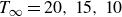 $T_\infty = 20,\,15,\,10$
and
$T_\infty = 20,\,15,\,10$
and
 $4^{\,\circ} \text{C}$
) and approximate ocean conditions of 34 ‰ (
$4^{\,\circ} \text{C}$
) and approximate ocean conditions of 34 ‰ (
 $T_\infty = 4$
and
$T_\infty = 4$
and
 $2^{\,\circ} \text{C}$
). A concomitant DNS mimicking the experimental set-up has been performed using both linear and nonlinear EoS for the water density. The BL velocity and temperature measurements show better agreement with the DNS that employed a nonlinear EoS, as compared with a linear EoS or the isothermal wall similarity solution. This indicates the importance of using the nonlinear EoS for numerical and analytical analysis. The flow is uni-directional for
$2^{\,\circ} \text{C}$
). A concomitant DNS mimicking the experimental set-up has been performed using both linear and nonlinear EoS for the water density. The BL velocity and temperature measurements show better agreement with the DNS that employed a nonlinear EoS, as compared with a linear EoS or the isothermal wall similarity solution. This indicates the importance of using the nonlinear EoS for numerical and analytical analysis. The flow is uni-directional for
 $S_\infty =0$
although a downward flow at
$S_\infty =0$
although a downward flow at
 $T_\infty = 20,\,15\text{ and }10^{\,\circ} \text{C}$
is replaced by an upward flow at
$T_\infty = 20,\,15\text{ and }10^{\,\circ} \text{C}$
is replaced by an upward flow at
 $T_\infty = 4^{\,\circ} \text{C}$
owing to density maximum at
$T_\infty = 4^{\,\circ} \text{C}$
owing to density maximum at
 $4^{\,\circ} \text{C}$
. The BL exhibits a more complicated bi-directional flow under ocean conditions of
$4^{\,\circ} \text{C}$
. The BL exhibits a more complicated bi-directional flow under ocean conditions of
 $S_\infty =34$
‰ at both
$S_\infty =34$
‰ at both
 $T_\infty = 4$
and
$T_\infty = 4$
and
 $2^{\,\circ} \text{C}$
. The inner salinity-driven fresh-melt-water flow is upwards, whereas the outer temperature-driven flow is downwards.
$2^{\,\circ} \text{C}$
. The inner salinity-driven fresh-melt-water flow is upwards, whereas the outer temperature-driven flow is downwards.
Inclusion of salinity does not always result in a bi-directional flow. We show that our experimental data match with the flow regime
 $({\varLambda },\,\textit{Le})$
diagram first proposed by Nilson (Reference Nilson1985), and that it is likely to be a more detailed indicator of flow regimes than the usual use of the
$({\varLambda },\,\textit{Le})$
diagram first proposed by Nilson (Reference Nilson1985), and that it is likely to be a more detailed indicator of flow regimes than the usual use of the
 $(T_\infty ,\, S_\infty )$
diagram. We also derived an equation that allows one to calculate the interface conditions (
$(T_\infty ,\, S_\infty )$
diagram. We also derived an equation that allows one to calculate the interface conditions (
 $T_i$
and
$T_i$
and
 $S_i$
) from given
$S_i$
) from given
 $T_\infty$
and
$T_\infty$
and
 $S_\infty$
(and other usual properties) that can predict the flow regimes on the
$S_\infty$
(and other usual properties) that can predict the flow regimes on the
 $({\varLambda },\,\textit{Le})$
diagram. For Antarctic conditions we observe that the laminar flow is mostly bi-directional although tending towards being driven more strongly by salinity rather than temperature. Importantly, bi-directional flow analysis shows that even though the density contribution of temperature is much smaller than that of the salinity, the net buoyancy, and hence the flow, is dictated by the volume over which buoyancy acts (
$({\varLambda },\,\textit{Le})$
diagram. For Antarctic conditions we observe that the laminar flow is mostly bi-directional although tending towards being driven more strongly by salinity rather than temperature. Importantly, bi-directional flow analysis shows that even though the density contribution of temperature is much smaller than that of the salinity, the net buoyancy, and hence the flow, is dictated by the volume over which buoyancy acts (
 $\approx {\varLambda } \textit{Le}^{1/2}$
). Since temperature has a larger BL thickness (owing to
$\approx {\varLambda } \textit{Le}^{1/2}$
). Since temperature has a larger BL thickness (owing to
 $\kappa _T \gg \kappa _S$
), the net buoyancy effects from both temperature and salinity are important. This volume effect is enhanced by the fact that the salinity BL is strongly constrained by the wall no-slip condition whereas the thermal BL is freer to evolve, which also leads to Nilson’s (Reference Nilson1985) bi-directional flow regime limits of
$\kappa _T \gg \kappa _S$
), the net buoyancy effects from both temperature and salinity are important. This volume effect is enhanced by the fact that the salinity BL is strongly constrained by the wall no-slip condition whereas the thermal BL is freer to evolve, which also leads to Nilson’s (Reference Nilson1985) bi-directional flow regime limits of
 ${\varLambda } \textit{Le}\approx 1$
and
${\varLambda } \textit{Le}\approx 1$
and
 ${\varLambda } \textit{Le}^{1/3} \approx 1$
.
${\varLambda } \textit{Le}^{1/3} \approx 1$
.
Uni- and bi-directional flow effects are also observed on the melt rates. Melt rates of the ice were quantified through three different experimental methods, and these measurements match reasonably well with the DNS rates. The thermally driven (
 $S_\infty =0$
) uni-directional flows behave as expected from the laminar scaling with height
$S_\infty =0$
) uni-directional flows behave as expected from the laminar scaling with height
 $z$
; the BL thickness and velocity respectively increase in the flow direction like
$z$
; the BL thickness and velocity respectively increase in the flow direction like
 $z^{1/4}$
and
$z^{1/4}$
and
 $z^{1/2}$
, whereas the melt rate
$z^{1/2}$
, whereas the melt rate
 $V\sim z^{-1/4}$
decreases. Conversely, the bi-directional flows do not adhere to these scalings and especially the melt-rate scaling. The inner salinity-driven BL scaling is affected by the oppositely growing outer thermal BL. Furthermore, the requirement for the melt rate to satisfy both the salinity and temperature fluxes means that interface conditions (
$V\sim z^{-1/4}$
decreases. Conversely, the bi-directional flows do not adhere to these scalings and especially the melt-rate scaling. The inner salinity-driven BL scaling is affected by the oppositely growing outer thermal BL. Furthermore, the requirement for the melt rate to satisfy both the salinity and temperature fluxes means that interface conditions (
 $S_i$
and
$S_i$
and
 $T_i$
) are not constant with
$T_i$
) are not constant with
 $z$
. The counteracting effects of salinity and temperature result in a more uniform
$z$
. The counteracting effects of salinity and temperature result in a more uniform
 $V$
with
$V$
with
 $z$
(unlike
$z$
(unlike
 $V$
decreasing with
$V$
decreasing with
 $z$
).
$z$
).
An implication for modelling is that one might predict a lower ice-shelf melting with
 $z$
based on the usual laminar BL scaling, if the effects of bi-directional flow are not recognised. Although the present work focuses only on laminar flow, it is more common for the BL to be modelled as a turbulent wall plume with a vertically distributed source of buoyancy (e.g. McConnochie & Kerr Reference McConnochie and Kerr2016b
). This assumption is fairly accurate when we consider upward buoyancy generated by relatively fresher water released from ice melting. Here the ice face acts as a vertically distributed source of buoyancy. Although it may sound reasonable to neglect thermal buoyancy effects because their contribution to density variation is very small, as noted herein, even with the relatively weaker contribution for the buoyancy, temperature variation can result in a larger buoyancy force even in the turbulent regime if turbulent diffusivities are dissimilar and downward buoyancy acts across a broader region outside of the salinity BL. In such a scenario, both upward and downward buoyancy generation (which acts as an upward buoyancy loss) should be considered to calculate the net upward buoyancy. Moreover, it is likely that these opposing buoyancy forces will also influence the melt-rate scaling. Therefore, future experimental studies in the turbulent flow regime are required to understand the role of opposing buoyancy in turbulent flow fields and its implications for modelling flow behaviour and ice melting dynamics.
$z$
based on the usual laminar BL scaling, if the effects of bi-directional flow are not recognised. Although the present work focuses only on laminar flow, it is more common for the BL to be modelled as a turbulent wall plume with a vertically distributed source of buoyancy (e.g. McConnochie & Kerr Reference McConnochie and Kerr2016b
). This assumption is fairly accurate when we consider upward buoyancy generated by relatively fresher water released from ice melting. Here the ice face acts as a vertically distributed source of buoyancy. Although it may sound reasonable to neglect thermal buoyancy effects because their contribution to density variation is very small, as noted herein, even with the relatively weaker contribution for the buoyancy, temperature variation can result in a larger buoyancy force even in the turbulent regime if turbulent diffusivities are dissimilar and downward buoyancy acts across a broader region outside of the salinity BL. In such a scenario, both upward and downward buoyancy generation (which acts as an upward buoyancy loss) should be considered to calculate the net upward buoyancy. Moreover, it is likely that these opposing buoyancy forces will also influence the melt-rate scaling. Therefore, future experimental studies in the turbulent flow regime are required to understand the role of opposing buoyancy in turbulent flow fields and its implications for modelling flow behaviour and ice melting dynamics.
While the present study provides detailed insights into the fundamentals of the BL dynamics, it is important to emphasise that, in the context of ice shelves, the direct relevance of these laminar flow findings is limited to the grounding line region, typically within the first few tens of centimetres along a vertical ice face. Beyond this region, turbulent mixing dominates, which can alter flow behaviour, buoyancy distribution and melt-rate scaling to a certain extent. Thus, the insights gained here should be interpreted and applied accordingly.
Acknowledgements
The authors gratefully acknowledge the Australian National Computational Infrastructure for providing the computational resources used in this study. The National Computational Infrastructure is supported by the Commonwealth of Australia and hosted at the Australian National University.
Funding
This research was supported by the Australian Research Council. B.G. was supported by Australian Research Council grants FT180100037, DP240102823, and SR200100008.
Declaration of interests
The authors report no conflict of interest.
Appendix A. Two-component laminar BL equations and the region of bi-directional flow
The purpose of this appendix is to start with the governing equations and provide a self-contained derivation of the limits of the bi-directional flow presented by Nilson (Reference Nilson1985) as well as to cover some background useful in §§ 2 and 6. See also Kuiken (Reference Kuiken1968), Nilson & Baer (Reference Nilson and Baer1982) and Wells & Worster (Reference Wells and Worster2011).
It is assumed that the interface temperature (
 $T_i$
) and salinity (
$T_i$
) and salinity (
 $S_i$
) as well as the far-field conditions (
$S_i$
) as well as the far-field conditions (
 $T_\infty$
and
$T_\infty$
and
 $S_\infty$
) are constant, and density depends linearly on
$S_\infty$
) are constant, and density depends linearly on
 $T$
and
$T$
and
 $S$
via the thermal expansion and haline contraction coefficient,
$S$
via the thermal expansion and haline contraction coefficient,
 $\alpha$
and
$\alpha$
and
 $\beta$
, respectively. For two-dimensional steady flow where diffusive effects are dominant only in the wall-normal (
$\beta$
, respectively. For two-dimensional steady flow where diffusive effects are dominant only in the wall-normal (
 $x$
) direction, the continuity, vertical (
$x$
) direction, the continuity, vertical (
 $z$
-direction) momentum, temperature and salt balance equations are
$z$
-direction) momentum, temperature and salt balance equations are
 \begin{align} \frac {\partial u}{\partial x} + \frac {\partial w}{\partial z} = 0 , \quad &u \frac {\partial w}{\partial x} + w \frac {\partial w}{\partial z} = \nu \frac {\partial ^2 w}{\partial x^2} - g\alpha (T_\infty -T) + g\beta (S_\infty -S), \end{align}
 \begin{align} u \frac {\partial T}{\partial x} + w \frac {\partial T}{\partial z} = \kappa _T \frac {\partial ^2 T}{\partial x^2} ,\quad &u \frac {\partial S}{\partial x} + w \frac {\partial S}{\partial z} = \kappa _S \frac {\partial ^2 S}{\partial x^2}, \end{align}
along with the boundary conditions:
 $ u(x=0) = 0$
,
$ u(x=0) = 0$
,
 $u(x \to \infty ) = 0$
,
$u(x \to \infty ) = 0$
,
 $w(x=0) = 0$
,
$w(x=0) = 0$
,
 $w(x \to \infty ) = 0$
,
$w(x \to \infty ) = 0$
,
 $ T(x=0) = T_i$
,
$ T(x=0) = T_i$
,
 $T(x \to \infty ) = T_{\infty }$
,
$T(x \to \infty ) = T_{\infty }$
,
 $S(x=0) = S_i$
and
$S(x=0) = S_i$
and
 $S(x \to \infty ) = S_{\infty }$
, where
$S(x \to \infty ) = S_{\infty }$
, where
 $u$
and
$u$
and
 $w$
are velocities in
$w$
are velocities in
 $x$
and
$x$
and
 $z$
directions. Since both
$z$
directions. Since both
 $\alpha$
and
$\alpha$
and
 $\beta$
are positive and
$\beta$
are positive and
 $T$
and
$T$
and
 $S$
are always smaller than their far-field values, temperature and salinity will, respectively, drive a downward and upward flow (see (A1b
)). Continuity is satisfied using the streamfunction
$S$
are always smaller than their far-field values, temperature and salinity will, respectively, drive a downward and upward flow (see (A1b
)). Continuity is satisfied using the streamfunction
 $\psi$
, such that
$\psi$
, such that
 $w=\partial \psi /\partial x$
and
$w=\partial \psi /\partial x$
and
 $u=-\partial \psi /\partial z$
. The partial differential equations (A1) are reduced to ordinary differential equations by defining non-dimensional quantities:
$u=-\partial \psi /\partial z$
. The partial differential equations (A1) are reduced to ordinary differential equations by defining non-dimensional quantities:
 \begin{equation} \tilde {x} \equiv \frac {x}{l_S}, \quad\tilde {\psi } \equiv \frac {\psi } {4 (\nu /l_S) z}, \quad\tilde {T}\equiv \frac {(T_\infty -T)}{( T_\infty -T_i)} \quad \textrm {and}\quad\tilde {S}\equiv \frac {(S_\infty -S)}{(S_\infty -S_i)}, \end{equation}
where salinity-based length scale
 $l_S := [4 \nu ^2 z/(g \beta (S_\infty -S_i))]^{1/4}$
. Here,
$l_S := [4 \nu ^2 z/(g \beta (S_\infty -S_i))]^{1/4}$
. Here,
 $T_i$
and
$T_i$
and
 $S_i$
are assumed to be independent of
$S_i$
are assumed to be independent of
 $z$
. We could have used a temperature-based length scale (say,
$z$
. We could have used a temperature-based length scale (say,
 $l_T$
) also, which we will consider later, but for now, we carry out the steps with
$l_T$
) also, which we will consider later, but for now, we carry out the steps with
 $l_S$
. (Note that except the factor of 4,
$l_S$
. (Note that except the factor of 4,
 $l_S$
can be obtained by balancing the viscous and salinity terms in (A1b
):
$l_S$
can be obtained by balancing the viscous and salinity terms in (A1b
):
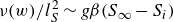 $\nu (w)/l_S^2 \sim g \beta (S_\infty -S_i)$
, and substituting
$\nu (w)/l_S^2 \sim g \beta (S_\infty -S_i)$
, and substituting
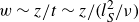 $w\sim z/t \sim z/(l_S^2/\nu )$
.) Using the non-dimensional quantities in (A2), (A1) becomes
$w\sim z/t \sim z/(l_S^2/\nu )$
.) Using the non-dimensional quantities in (A2), (A1) becomes
 \begin{align} &\frac { {\rm d}^3 \tilde {\psi }}{\textrm {d}\tilde {x}^3} + \tilde {S} - {\varLambda } \, \tilde {T} - 2 \left (\frac {\textrm {d} \tilde {\psi }}{\textrm {d}\tilde {x}}\right )^{{\kern-2pt}2} + 3\, \tilde {\psi }\, \frac { {\rm d}^2 \tilde {\psi }}{\textrm {d}\tilde {x}^2} = 0, \end{align}
 \begin{align} &\frac { {\rm d}^2 \tilde {T}}{\textrm {d}\tilde {x}^2} + 3 \,\textit{Pr} \,\tilde {\psi }\, \frac {\textrm {d} \tilde {T}}{\textrm {d}\tilde {x}} = 0,\quad \frac { {\rm d}^2 \tilde {S}}{\textrm {d}\tilde {x}^2} + 3\, \textit{Sc}\, \tilde {\psi }\, \frac {\textrm {d} \tilde {S}}{\textrm {d}\tilde {x}} = 0, \end{align}
where
 ${\varLambda } \equiv \alpha (T_\infty -T_i)/\beta (S_\infty -S_i)$
and Prandtl and Schmidt numbers are
${\varLambda } \equiv \alpha (T_\infty -T_i)/\beta (S_\infty -S_i)$
and Prandtl and Schmidt numbers are
 $\textit{Pr}=\nu /\kappa _T$
and
$\textit{Pr}=\nu /\kappa _T$
and
 $\textit{Sc}=\nu /\kappa _S$
(see (2.1) and (2.2)). The first term in (A3a
) is the viscous term and next two are salinity driving upward flow and temperature driving downward flow. If this was a single-component flow, i.e. either
$\textit{Sc}=\nu /\kappa _S$
(see (2.1) and (2.2)). The first term in (A3a
) is the viscous term and next two are salinity driving upward flow and temperature driving downward flow. If this was a single-component flow, i.e. either
 $\tilde {T}$
or
$\tilde {T}$
or
 $\tilde {S}$
is zero, then the remaining two equations can be solved for a given either
$\tilde {S}$
is zero, then the remaining two equations can be solved for a given either
 $\textit{Pr}$
or
$\textit{Pr}$
or
 $\textit{Sc}$
, as carried out numerically by Ostrach (Reference Ostrach1952). For two-component flow, the new control parameter
$\textit{Sc}$
, as carried out numerically by Ostrach (Reference Ostrach1952). For two-component flow, the new control parameter
 $\varLambda$
emerges, along with
$\varLambda$
emerges, along with
 $\textit{Le} = \textit{Sc}/\textit{Pr} = \kappa _T/\kappa _S$
that is
$\textit{Le} = \textit{Sc}/\textit{Pr} = \kappa _T/\kappa _S$
that is
 $O(100)$
and hence assumed ‘large’.
$O(100)$
and hence assumed ‘large’.
When both salinity and temperature as opposing forces are present, one can obtain a uni-directional upward or downward flow if, respectively,
 $\tilde {S}$
or
$\tilde {S}$
or
 $\tilde {T}$
is dominant, or the possibility of bi-directional flow appears when
$\tilde {T}$
is dominant, or the possibility of bi-directional flow appears when
 $\tilde {S}$
and
$\tilde {S}$
and
 $\tilde {T}$
through
$\tilde {T}$
through
 $R$
become equally important. To identify the boundary of this bi-directional flow, Nilson (Reference Nilson1985) starts with the analysis of Kuiken (Reference Kuiken1968) that we follow now. In accordance with the case considered here, a large
$R$
become equally important. To identify the boundary of this bi-directional flow, Nilson (Reference Nilson1985) starts with the analysis of Kuiken (Reference Kuiken1968) that we follow now. In accordance with the case considered here, a large
 $\textit{Le}$
is assumed, which implies a thinner salinity BL closer to the ice sheet and a much thicker
$\textit{Le}$
is assumed, which implies a thinner salinity BL closer to the ice sheet and a much thicker
 $O(10)$
temperature BL. There are two limiting boundaries for the bi-directional flow: first, where the dominant upward uni-directional flow owing to
$O(10)$
temperature BL. There are two limiting boundaries for the bi-directional flow: first, where the dominant upward uni-directional flow owing to
 $\tilde {S}$
closer to the wall starts to be affected by the slowly emerging downward
$\tilde {S}$
closer to the wall starts to be affected by the slowly emerging downward
 $\tilde {T}$
flow; and second, where the dominant downward uni-directional
$\tilde {T}$
flow; and second, where the dominant downward uni-directional
 $\tilde {T}$
flow begins to be affected by the slowly emerging upward
$\tilde {T}$
flow begins to be affected by the slowly emerging upward
 $\tilde {S}$
flow closest to the wall.
$\tilde {S}$
flow closest to the wall.
First consider the dominant upward flow due to
 $\tilde {S}$
. Close to the wall (called the ‘inner’ flow in the asymptotic matching), the balance in (A3a
) is between the first two terms, and temperature is almost equal to
$\tilde {S}$
. Close to the wall (called the ‘inner’ flow in the asymptotic matching), the balance in (A3a
) is between the first two terms, and temperature is almost equal to
 $T_i$
, which implies that we can ignore the first equation in (A3b
) and the two terms in the second equation in (A3b
) should balance each other. To find the
$T_i$
, which implies that we can ignore the first equation in (A3b
) and the two terms in the second equation in (A3b
) should balance each other. To find the
 $\textit{Sc}$
scaling that will achieve these two balances, consider
$\textit{Sc}$
scaling that will achieve these two balances, consider
 $\tilde {\psi } = (\textit{Sc})^a f(\eta )$
and
$\tilde {\psi } = (\textit{Sc})^a f(\eta )$
and
 $\tilde {x} = (\textit{Sc})^b \eta$
, where
$\tilde {x} = (\textit{Sc})^b \eta$
, where
 $f$
and
$f$
and
 $\eta$
are the new non-dimensional streamfunction and distance. Substituting these expressions to balance the first two terms in (A3a
) and two terms in (A3b
) will provide two equations for
$\eta$
are the new non-dimensional streamfunction and distance. Substituting these expressions to balance the first two terms in (A3a
) and two terms in (A3b
) will provide two equations for
 $a$
and
$a$
and
 $b$
, which when solved results in
$b$
, which when solved results in
 \begin{equation} \tilde {\psi } = \textit{Sc}^{-3/4} f(\eta )\quad\textrm {and}\quad \tilde {x} = \textit{Sc}^{-1/4} \eta . \end{equation}
Substituting (A4) in (A3a
) (neglecting the two advection terms) with
 $\textit{Le} \gg 1$
and
$\textit{Le} \gg 1$
and
 $\varLambda \ll 1$
and into the second equation of (A3b
) results in
$\varLambda \ll 1$
and into the second equation of (A3b
) results in
 \begin{equation} f_{\eta \eta \eta } + \tilde {S} = 0, \quad \tilde {S}_{\eta \eta } + 3{\kern-1pt}f{\kern-1pt}\tilde{S}_{\eta } = 0 \quad\textrm {and}\quad \tilde {T}=1, \end{equation}
where subscript
 $\eta $
denotes differentiation with respect to
$\eta $
denotes differentiation with respect to
 $\eta$
. This dominant upward flow will be counteracted by a downward flow when temperature becomes important, especially in the ‘outer’ region. A simplified set of equations similar to (A5) for temperature can be derived from (A1) if we use
$\eta$
. This dominant upward flow will be counteracted by a downward flow when temperature becomes important, especially in the ‘outer’ region. A simplified set of equations similar to (A5) for temperature can be derived from (A1) if we use
 $l_T := [4 \nu ^2 z/(g \alpha (T_\infty -T_i))]^{1/4}$
in (A2), i.e.
$l_T := [4 \nu ^2 z/(g \alpha (T_\infty -T_i))]^{1/4}$
in (A2), i.e.
 \begin{equation} \tilde {x}^* \equiv \frac {x}{l_T}, \quad\tilde {\psi }^* \equiv \frac {\psi }{4 (\nu /l_T) z}, \end{equation}
and substitute
 $\textit{Pr}$
for
$\textit{Pr}$
for
 $\textit{Sc}$
in (A4), i.e.
$\textit{Sc}$
in (A4), i.e.
 $\tilde {\psi }^* = \textit{Pr}^{-3/4} f^*(\eta ^*)\textrm { and } \tilde {x}^* = \textit{Pr}^{-1/4} \eta ^*$
, which will result in (with
$\tilde {\psi }^* = \textit{Pr}^{-3/4} f^*(\eta ^*)\textrm { and } \tilde {x}^* = \textit{Pr}^{-1/4} \eta ^*$
, which will result in (with
 $\textit{Pr} \gg 1$
)
$\textit{Pr} \gg 1$
)
 \begin{equation} f^*_{\eta ^*\eta ^*\eta ^*} - \tilde {T} = 0, \quad \tilde {T}_{\eta ^*\eta ^*} + 3\,f^*\,\tilde {T}_{\eta ^*} = 0 \quad \textrm {and}\quad \tilde {S}=0. \end{equation}
The last equation in (A7) reflects that, in the outer region, salinity is at the far-field value. The dominant terms in the solutions of (A5) and (A7) are
 $f \sim a_0 + a_1\eta + a_2\eta ^2$
for
$f \sim a_0 + a_1\eta + a_2\eta ^2$
for
 $\eta \gg 1$
and
$\eta \gg 1$
and
 $f^*\sim b_0 + b_1\eta ^* + b_2\eta ^{*2}$
for
$f^*\sim b_0 + b_1\eta ^* + b_2\eta ^{*2}$
for
 $\eta ^* \ll 1$
, with constant
$\eta ^* \ll 1$
, with constant
 $a$
and
$a$
and
 $b$
. Matching of the two solutions of (A5) and (A7) implies that streamfunctions in the limit
$b$
. Matching of the two solutions of (A5) and (A7) implies that streamfunctions in the limit
 $\eta \to \infty$
and
$\eta \to \infty$
and
 $\eta ^* \to 0$
should match (noting that
$\eta ^* \to 0$
should match (noting that
 $\eta ^*/\eta = ({\varLambda }/\textit{Le})^{1/4}$
):
$\eta ^*/\eta = ({\varLambda }/\textit{Le})^{1/4}$
):
 \begin{align} \lim _{\eta \to \infty } f \,{4 (\nu /l_S) z} \,\textit{Sc}^{-3/4} &= \lim _{\eta ^* \to 0} f^* \,{4 (\nu /l_T) z} \, \textit{Pr}^{-3/4} \nonumber \\ \lim _{\eta \to \infty } f &= \left ( {\varLambda }\,\textit{Le}^3 \right )^{1/4}\lim _{\eta ^* \to 0} f^* , \end{align}
 \begin{align} a_0 + a_1\eta + a_2\eta ^2 &= \left ( {\varLambda }\,\textit{Le} \right )^{1/2} \left ( \frac {b_0}{({\varLambda }/\textit{Le})^{1/4}} + b_1 \eta + b_2 \eta ^2 ({\varLambda }/\textit{Le})^{1/4} \right )\!. \end{align}
The above equation is Nilson’s (Reference Nilson1985) equation (34). Now, keeping
 ${\varLambda }\,\textit{Le}$
fixed and letting
${\varLambda }\,\textit{Le}$
fixed and letting
 $\textit{Le} \to \infty$
, shows
$\textit{Le} \to \infty$
, shows
 $a_1 = ( {\varLambda }\,\textit{Le} )^{1/2} b_1$
that matches the velocity. Consistently, the numerical calculations of Nilson & Baer (Reference Nilson and Baer1982) show that the dominant upward flow owing to salinity is ‘disturbed’ by the incipient temperature-driven downward flow when
$a_1 = ( {\varLambda }\,\textit{Le} )^{1/2} b_1$
that matches the velocity. Consistently, the numerical calculations of Nilson & Baer (Reference Nilson and Baer1982) show that the dominant upward flow owing to salinity is ‘disturbed’ by the incipient temperature-driven downward flow when
 \begin{equation} {\varLambda }\,\textit{Le} \approx 1. \end{equation}
A similar analysis has been carried out by Nilson (Reference Nilson1985) to estimate the other boundary where the dominant downward flow owing to temperature starts to be countered by the incipient salinity-driven upward flow. The analysis starts by assuming
 $z$
as positive in the downward direction. The main flow (
$z$
as positive in the downward direction. The main flow (
 $f^*$
) is temperature-driven with a no-slip boundary condition at the ice face, i.e.
$f^*$
) is temperature-driven with a no-slip boundary condition at the ice face, i.e.
 $f^*_{\eta ^*}=0$
. Note that this is different from the above analysis where the velocity
$f^*_{\eta ^*}=0$
. Note that this is different from the above analysis where the velocity
 $f^*_{\eta ^*}$
was matched with dominant upward flow. A similar solution to incipient salinity-driven upward flow is obtained, and matching of the two solutions occurs for
$f^*_{\eta ^*}$
was matched with dominant upward flow. A similar solution to incipient salinity-driven upward flow is obtained, and matching of the two solutions occurs for
 $\eta \to \infty$
and
$\eta \to \infty$
and
 $\eta ^* \to 0$
, the same as (A8a
):
$\eta ^* \to 0$
, the same as (A8a
):
 \begin{align} \lim _{\eta \to \infty } f &= \left ( {\varLambda }\,\textit{Le}^3 \right )^{1/4}\lim _{\eta ^* \to 0} f^* , \end{align}
 \begin{align} a_0 + a_1\eta + a_2\eta ^2 &= \left ( {\varLambda }\,\textit{Le}^{1/3} \right )^{{3/4}} \left ( \frac {b_0}{({\varLambda }/\textit{Le})^{1/2}} + \frac {b_1}{({\varLambda }/\textit{Le})^{1/4}} \eta + b_2 \eta ^2 \right )\!. \end{align}
Forcing the wall velocity to be zero requires the coefficient of
 $\eta$
to be zero and the coefficient of
$\eta$
to be zero and the coefficient of
 $\eta ^2$
to be non-zero, resulting in
$\eta ^2$
to be non-zero, resulting in
 $a_2 = ({\varLambda }\,\textit{Le}^{1/3} )^{1/4} b_2$
, which shows that in a dominant downward temperature-driven flow the incipient upward salinity flow becomes important when
$a_2 = ({\varLambda }\,\textit{Le}^{1/3} )^{1/4} b_2$
, which shows that in a dominant downward temperature-driven flow the incipient upward salinity flow becomes important when
 \begin{equation} {\varLambda }\,\textit{Le}^{1/3} \approx 1, \end{equation}
which is the other boundary for bi-directional flow.
Appendix B. Effects of MTV/MTT chemicals on freezing point
Molecular tagging-based techniques described in § 3.2 require dissolving various chemical components in water to introduce phosphorescence properties to the solution. The freezing point of pure water is usually taken as
 $0^{\,\circ} \text{C}$
, and for saltwater the freezing point depression equation
$0^{\,\circ} \text{C}$
, and for saltwater the freezing point depression equation
 $T_i=a_s S_i$
is used. But the MTV/MTT chemical components also have the potential to change the freezing point of pure water based on Blagden’s law (e.g. Zumdahl, Zumdahl & DeCoste Reference Zumdahl, Zumdahl and DeCoste2020). Blagden’s law is given by
$T_i=a_s S_i$
is used. But the MTV/MTT chemical components also have the potential to change the freezing point of pure water based on Blagden’s law (e.g. Zumdahl, Zumdahl & DeCoste Reference Zumdahl, Zumdahl and DeCoste2020). Blagden’s law is given by
 \begin{equation} \Delta T_{\!f}=K_{\!f} m_{\textit{solute}} ,\end{equation}
where
 $\Delta T_{\!f}$
is the decrease in freezing point,
$\Delta T_{\!f}$
is the decrease in freezing point,
 $K_{\!f}$
is the cryoscopic constant and
$K_{\!f}$
is the cryoscopic constant and
 $m_{\textit{solute}}$
is the molarity of solutes. Here
$m_{\textit{solute}}$
is the molarity of solutes. Here
 $K_{\!f}$
depends on solvent and is
$K_{\!f}$
depends on solvent and is
 $1.86\rm \, K\,kg\,mol^{- 1}$
for water. In the MTV/MTT solution used in this study the total molarity of the components is
$1.86\rm \, K\,kg\,mol^{- 1}$
for water. In the MTV/MTT solution used in this study the total molarity of the components is
 $0.05031\,\rm mol\,kg^{- 1}$
which is mainly contributed by cyclohexanol (§ 3.2). Therefore, from (B1) we can calculate
$0.05031\,\rm mol\,kg^{- 1}$
which is mainly contributed by cyclohexanol (§ 3.2). Therefore, from (B1) we can calculate
 $\Delta T_{\!f}$
as
$\Delta T_{\!f}$
as
 $0.093^{\,\circ} \text{C}$
. Since the ambient temperatures in this study are much larger than this value, the resulting maximum thermal driving (
$0.093^{\,\circ} \text{C}$
. Since the ambient temperatures in this study are much larger than this value, the resulting maximum thermal driving (
 $T_\infty -T_i$
) change is only
$T_\infty -T_i$
) change is only
 $2\,\%$
, which is ignored.
$2\,\%$
, which is ignored.
Appendix C. The MTT calibration and adaptation
C.1. The MTT calibration procedure
Before actual experiments with the ice block are conducted, a calibration curve that relates
 $\tau$
to temperature is obtained using the same set-up. During the calibration process, the temperature of the water tank is varied from
$\tau$
to temperature is obtained using the same set-up. During the calibration process, the temperature of the water tank is varied from
 $0$
to
$0$
to
 $22^{\,\circ} \text{C}$
. These temperatures are measured using a thermistor with an accuracy of
$22^{\,\circ} \text{C}$
. These temperatures are measured using a thermistor with an accuracy of
 $0.05\,^{\circ}{\rm C}$
and a resolution of
$0.05\,^{\circ}{\rm C}$
and a resolution of
 $0.01^{\,\circ} \text{C}$
. The temperature increase for calibration is obtained by pre-cooling the solution in a refrigerator and allowing the solution to heat up naturally; then, the calibration was carried out outside the cold room. For low-
$0.01^{\,\circ} \text{C}$
. The temperature increase for calibration is obtained by pre-cooling the solution in a refrigerator and allowing the solution to heat up naturally; then, the calibration was carried out outside the cold room. For low-
 $T_\infty$
experiments, however, the cold room is used for calibration. During calibration the solution is stirred continuously using a magnetic stirrer to ensure the temperature inside the water tank is homogeneous and to avoid any photobleaching of the solution. Photobleaching can happen if the laser hits the same region of the fluid repeatedly over a long period such as during a calibration procedure. While the temperature of the water tank is increasing, phosphorescent images (25 image pairs) are obtained for different temperatures, and the thermistor reading is recorded for each temperature. After that, these image pairs are processed, and the time constant (
$T_\infty$
experiments, however, the cold room is used for calibration. During calibration the solution is stirred continuously using a magnetic stirrer to ensure the temperature inside the water tank is homogeneous and to avoid any photobleaching of the solution. Photobleaching can happen if the laser hits the same region of the fluid repeatedly over a long period such as during a calibration procedure. While the temperature of the water tank is increasing, phosphorescent images (25 image pairs) are obtained for different temperatures, and the thermistor reading is recorded for each temperature. After that, these image pairs are processed, and the time constant (
 $\tau$
) of the phosphorescent decay is calculated for each pixel along the tagged lines (as described in § 3.2). These
$\tau$
) of the phosphorescent decay is calculated for each pixel along the tagged lines (as described in § 3.2). These
 $\tau$
values are then averaged along the tagged line as well as across 25 image pairs, and these averaged
$\tau$
values are then averaged along the tagged line as well as across 25 image pairs, and these averaged
 $\tau$
values are used to obtain the calibration curve that relates
$\tau$
values are used to obtain the calibration curve that relates
 $\tau$
and temperature. Figure 12(a) shows a sample set of calibration curves obtained in the same constant-temperature bath with a second image exposure of 1, 2 and 3 ms. Data points of these curves are obtained by changing the second image exposure of the camera at each temperature. From figure 12(a) it can be observed that these curves are almost identical with small vertical shifts. For each MTT temperature measurement, a calibration curve with the same second image exposure is used.
$\tau$
and temperature. Figure 12(a) shows a sample set of calibration curves obtained in the same constant-temperature bath with a second image exposure of 1, 2 and 3 ms. Data points of these curves are obtained by changing the second image exposure of the camera at each temperature. From figure 12(a) it can be observed that these curves are almost identical with small vertical shifts. For each MTT temperature measurement, a calibration curve with the same second image exposure is used.
(a) The calibration curves obtained for second image exposures of 1 ms (red circles and solid line), 2 ms (green squares and dashed line) and 3 ms (blue triangles and dotted line) in the range
 $0{-}25^{\,\circ} \text{C}$
. Lines represent second-order polynomial fits to data. (b) The correction of calibration curves. (c) A sample image pair that was obtained during melt rate measurements by imaging the interface with
$0{-}25^{\,\circ} \text{C}$
. Lines represent second-order polynomial fits to data. (b) The correction of calibration curves. (c) A sample image pair that was obtained during melt rate measurements by imaging the interface with
 $T_\infty =10^{\,\circ} \text{C}$
and
$T_\infty =10^{\,\circ} \text{C}$
and
 $S_\infty =0$
: (i)
$S_\infty =0$
: (i)
 $t=60$
s and (ii)
$t=60$
s and (ii)
 $t=240$
s after placing the ice block in water.
$t=240$
s after placing the ice block in water.

C.2. Correction of calibration curves
After conducting the actual experiments using the ice block, in situ pre- and post-calibration image pairs are obtained for the fixed
 $T_0$
values. This was done because there is a chance that the calibration curve might have changed slightly from the original calibration due to the ageing of the solution and other unknown reasons, and these post- and pre-calibration points can be used to ‘correct’ the calibration curves to obtain accurate temperature measurements. The correction can be done using two methods. Typically, the change in the calibration curve due to ageing and other reasons (Hu & Koochesfahani Reference Hu and Koochesfahani2006) shifts the curve along the vertical axis. Therefore, the original curve (
$T_0$
values. This was done because there is a chance that the calibration curve might have changed slightly from the original calibration due to the ageing of the solution and other unknown reasons, and these post- and pre-calibration points can be used to ‘correct’ the calibration curves to obtain accurate temperature measurements. The correction can be done using two methods. Typically, the change in the calibration curve due to ageing and other reasons (Hu & Koochesfahani Reference Hu and Koochesfahani2006) shifts the curve along the vertical axis. Therefore, the original curve (
 $C$
) is shifted vertically such that it passes through the post-calibration data point as
$C$
) is shifted vertically such that it passes through the post-calibration data point as
 \begin{equation} C_{\textit{corrected}}= C+ \epsilon , \end{equation}
where the shift
 $\epsilon = \tau _c -\tau _0$
. Here
$\epsilon = \tau _c -\tau _0$
. Here
 $\tau _c$
is the time constant that the existing calibration curve (
$\tau _c$
is the time constant that the existing calibration curve (
 $C$
) gives for the temperature (
$C$
) gives for the temperature (
 $T_0$
) at pre- or post-calibration point is obtained, whereas
$T_0$
) at pre- or post-calibration point is obtained, whereas
 $\tau _0$
is the actual time constant measured at
$\tau _0$
is the actual time constant measured at
 $T_0$
during pre- or post-calibration.
$T_0$
during pre- or post-calibration.
The second method is normalising the original curve using the time constant corresponding to the temperature at which the calibration point is obtained (
 $\tau _c$
) and obtaining the new curve by multiplying the normalised curve by the actual time constant measured at the pre- or post-calibration point (
$\tau _c$
) and obtaining the new curve by multiplying the normalised curve by the actual time constant measured at the pre- or post-calibration point (
 $\tau _0$
) which can be described as
$\tau _0$
) which can be described as
 \begin{equation} C_{\textit{corrected}}= \frac {C}{\tau _c} \times \tau _0. \end{equation}
Utilisation of the normalised curve to avoid the ageing effects is described in Hu & Koochesfahani (Reference Hu and Koochesfahani2006). Figure 12(b) shows a comparison between original, shifted and normalised calibration curves. Here it can be observed that both the correction methods give almost identical corrected curves. This study, however, uses the method of normalising the original curve to obtain the corrected curve.
C.3. Molecular tagging thermometry in saltwater
For saltwater, separate calibration curves are obtained. From the experiments, however, it was observed that introducing salt to the water has an effect on the calibration curve similar to the ageing effect. Predominately, salt also causes the calibration curve to shift vertically. Therefore, the same procedure of post-calibration can be followed for saltwater as well if the salinity remains constant. When ice is melting, a salinity BL forms near the interface where the salinity is not constant. Therefore, using the same calibration curve within the salinity BL may give erroneous results. Salt, however, has a very small diffusivity (compared with temperature), and the thickness of the salt BL is very small compared with the thermal BL. For all the cases that used salt, the thickness of the salinity BL was smaller than 1 mm. Therefore, temperature measurements within this region are ignored.
Appendix D. Image processing
Matlab is used to pre-process raw images obtained from the camera. To remove any fixed pattern noise in the images (to eliminate the effect of pixel-to-pixel variation of camera sensitivity), two sets of images are obtained using the camera prior to the experiments. The first set of images is acquired by imaging a uniformly illuminated screen using the camera (flat-field images), while the second set is obtained when there is no incident light on the camera sensor (dark-field images). Using the following equation, these flat-field and dark-field images are then used to obtain the corrected signal from each pixel:
 \begin{equation} \textrm {Corrected image}= \frac {(\textrm {Raw image}) - (\textrm {Dark-field image})}{(\textrm {Flat-field image}) - (\textrm {Dark-field image})} .\end{equation}
After that, the next step is selecting a region of interest in the image that contains the tagged line and applying a two-dimensional spatial filter to reduce noise levels in the images. Here, the choice of filtering type is important to a certain degree, especially for MTT, although all box, median and Gaussian filters give acceptable results for MTV. After trying different types of filters, we found that filters that preserve the sharpness of the edges have the best performance because median and box filters usually smooth the intensity peak of the tagged line and consequently change the time constant
 $\tau$
. Therefore, in this study, a two-dimensional guided filter (He, Sun & Tang Reference He, Sun and Tang2012) is used to reduce the noise level in the image. Guided filtering is an edge-preserving filtering technique where statistics (mean and variance) of the region being filtered are taken into account when calculating the value of the output pixel. It smooths flat regions similar to Gaussian filters, preserving the intensity peak in the images (without over-smoothing the peak). Filter window size used in MTV is
$\tau$
. Therefore, in this study, a two-dimensional guided filter (He, Sun & Tang Reference He, Sun and Tang2012) is used to reduce the noise level in the image. Guided filtering is an edge-preserving filtering technique where statistics (mean and variance) of the region being filtered are taken into account when calculating the value of the output pixel. It smooths flat regions similar to Gaussian filters, preserving the intensity peak in the images (without over-smoothing the peak). Filter window size used in MTV is
 $20\times 20$
and in MTV is
$20\times 20$
and in MTV is
 $3\times 20$
. Filter size does not significantly affect the mean of both temperature and velocity measurements. It is important to apply the same filtering for both the calibration and measurement images to ensure temperature measurements are not affected by change of
$3\times 20$
. Filter size does not significantly affect the mean of both temperature and velocity measurements. It is important to apply the same filtering for both the calibration and measurement images to ensure temperature measurements are not affected by change of
 $\tau$
due to different filtering.
$\tau$
due to different filtering.
Appendix E. Melt-rate measurements
E.1. Method 1: imaging the interface
One of the two methods utilised in this study to obtain melt-rate measurements is imaging the interface described in § 3.5 where the position of the ice–water interface is tracked as shown in figure 12(ci) and 12(cii). The window size of the imaging is
 $23$
mm
$23$
mm
 $\times$
 $23$
mm in this set-up, and the bottom of the window is at
$23$
mm in this set-up, and the bottom of the window is at
 $z=10$
mm. Images are captured with a frequency of 5 f.p.s. in single-image mode. In order to calculate the ice melting rates using the images, all the images are pre-processed so that the ice–water interface can be easily detected. First, the region of interest in the image is selected, and the contrast of the image is adjusted. After that, the image is converted to a binary image. Then, a second-order polynomial is fitted along the edge that indicates the ice–water interface and the ice melting rate is calculated by measuring the shift of this line in two images because the time difference between these two images is known.
$z=10$
mm. Images are captured with a frequency of 5 f.p.s. in single-image mode. In order to calculate the ice melting rates using the images, all the images are pre-processed so that the ice–water interface can be easily detected. First, the region of interest in the image is selected, and the contrast of the image is adjusted. After that, the image is converted to a binary image. Then, a second-order polynomial is fitted along the edge that indicates the ice–water interface and the ice melting rate is calculated by measuring the shift of this line in two images because the time difference between these two images is known.
In this study, when calculating the melt rates, 10 images captured during
 $t$
= 60–62 s period and 10 images captured during 120–122 s are used as 10 image pairs so that the two images are captured with a 60 s delay in each image pair. Using this procedure averaged melt-rate profiles are obtained along the
$t$
= 60–62 s period and 10 images captured during 120–122 s are used as 10 image pairs so that the two images are captured with a 60 s delay in each image pair. Using this procedure averaged melt-rate profiles are obtained along the
 $z$
axis of about
$z$
axis of about
 $23$
mm.
$23$
mm.
E.2. Method 2: molecular tagging melt-rate measurements
In this section, we explain the method to detect the receding ice face using the laser tag lines in MTV/MTT phosphorescent images and quantify the ice melt rate. When acquiring phosphorescence images for MTV and MTT measurements, the laser passes through the water and impinges on the ice–water interface perpendicularly. When the phosphorescence intensity along the line is considered, it smoothly attenuates in the water but attenuates markedly when passing through ice. However, a relatively high intensity increase can be observed at the ice–water interface. This is likely due to the scattering of light when the beam hits the interface. This phenomenon can be seen in the phosphorescence images in figure 4(ai). This high-intensity region is used to identify the ice–water interface position on the images.
At first, the maximum intensity pixels along the tagged line of the first image of each image pair are obtained. Then, all these intensity lines were obtained for each image pair with increasing time as visualised in figure 4(b) (where the colour shows phosphorescence intensity). This map gives space and time information on the ice–water interface. In this figure, the movement of the interface can be clearly identified using the high-intensity trace. The ice-face location is obtained by the maximum intensity gradient at the interface, and it is shown using a dark line in figure 4(b). Usually, the melt rate quickly reaches a steady-state value and becomes time-independent. Therefore, the trace line is straight with a constant slope
 $m$
(px/image). Since the actual length-to-pixel ratio
$m$
(px/image). Since the actual length-to-pixel ratio
 $r$
(mm/px) is known through MTV calibration and the frequency of the data acquisition
$r$
(mm/px) is known through MTV calibration and the frequency of the data acquisition
 $f$
(Image s−1) is fixed, the ice ablation velocity
$f$
(Image s−1) is fixed, the ice ablation velocity
 $V$
can be calculated as
$V$
can be calculated as
 \begin{equation} V= \textit{rfm}. \end{equation}
A comparison between results obtained using this method and others is shown in figure 10, and they are in reasonable agreement with each other.
The main advantages of this method are that a separate set of experiments is not required, and the melt rate can be estimated using the same images used for MTV and MTT. The other advantage is that melt rates can be measured simultaneously with velocity and temperature measurements. This is useful when studying how velocity and temperature affect melt rate because this method is less susceptible to experiment-to-experiment variations. Finally, the image processing to detect the interface is less complex compared with the method of directly imaging the interface, which can result in lower errors in the laser line method. A drawback of this method is the lack of space resolution along the interface height. In the present study, laser lines are targeted at only one location (or at a maximum of three), whereas directly imaging the interface provides
 $V$
profile within the imaging window.
$V$
profile within the imaging window.


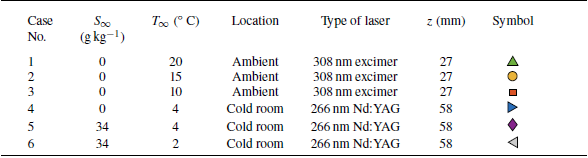


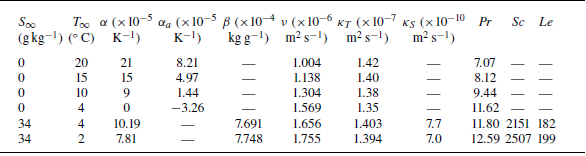


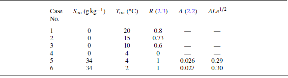


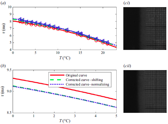


 Open access