


Introduction
Whether political parties want power for power’s sake or as a means of implementing their preferred policy, an instrumental desire to win elections is typically expected to drive their strategic behavior. Yet, parties sometimes appear to deviate from this law of electoral politics. The most prominent example is the case of Barry Goldwater, Republican candidate in the 1964 presidential elections. Goldwater ran on an extreme right-wing platform, despite the widespread belief that such platform would be too unpopular with the American public to be electorally viable. Goldwater himself admitted he never expected to win (Goldwater Reference Goldwater1988, 154). Indeed, he lost to Lyndon Johnson in a landslide victory.
This and other examples suggest that political parties sometimes choose to settle for electoral defeat: they adopt unpopular positions, even if this means losing the upcoming election for sure. From a rational choice perspective, this seems puzzling. Existing models predict that instrumentally rational parties will not sow the seeds of their own demise. Even if a party is motivated solely by ideology, it should never accept certain electoral defeat. Indeed, extant explanations for these and other cases rely on the assumption that parties (i.e., their members, activists, or candidates themselves) have expressive rather than strategic motivations and value ideological purity. Thus, a party may be willing to lose if winning comes at purity’s expense (Budge, Ezrow, and McDonald Reference Budge, Ezrow and McDonald2010; Harmel and Janda Reference Harmel and Janda1994; Roemer Reference Roemer2009; Strom Reference Strom1990).
This paper’s main contribution is to show that ideologically motivated parties may instead choose to lose for entirely strategic reasons, even without expressive concerns for purity. A party whose ideology is unpopular with the electorate faces a trade-off between compromising to win the upcoming election and changing the voters’ preferences to be able to win with a better platform in the future. Under some conditions, the party gambles on the future: chooses to lose today to change voters’ views and win big tomorrow. Crucially, one such condition is that parties are ideological not only in their preferences but also in their beliefs about which policy is best for voters. Thus, this paper shows that phenomena typically ascribed to expressive motivations can instead arise from strategic considerations coupled with behavioral tendencies such as parties agreeing to disagree.
To provide a microfoundation for this intuition, I analyze a model of repeated spatial elections with two periods. In each period, two policy-motivated parties compete for the support of a representative voter by proposing a platform along the left–right spectrum. The voter elects the party whose platform provides her with the highest expected payoff. The model introduces two novel features. First, the voter (and both parties) are uncertain about which policy is best for her. Here, players face what Tavits (Reference Tavits2007) defines as pragmatic policy issues and are unsure of “what types of policies are related to what sorts of outcomes” (155). Their uncertainty thus refers to the expected consequences of the various policies. For example, high taxation may be good for the representative voter, as it improves the provision of public goods, or bad for her, if it hampers economic growth. Second, the players hold different prior beliefs about which policy is best for the voter. In my setup, these priors represent a second dimension of ideology: the players’ “political beliefs systems” (Sartori Reference Sartori1969, 400). Going back to our redistribution example, a left-wing party believes the net effect of government intervention to be positive for the average voter, whereas a right-wing one is convinced of the virtues of trickle-down economics. Importantly, my players recognize that they hold different worldviews but do not infer anything from the existence of this disagreement: they agree to disagree.
In this setting, the voter’s preferences may change as she experiences the consequences of the first-period implemented policy:Footnote 1 she observes how much she liked (or disliked) this policy’s outcome and revises her expectation over the location of the optimal platform. However, policy outcomes are noisy—that is, their realization is subject to an idiosyncratic shock. This complicates the voter’s inference problem. A consequence of this technology, I show, is that the voter learns more about her ideal policy when more radical platforms (i.e., platforms farther away from the center of the ideological policy space) are enacted. Formally, radical platforms make it easier for the voter to separate information from noise. Substantively, suppose that following the implementation of a radical progressive platform, involving very high taxation and public spending, the voter sees her condition improve. Then, she infers that this platform is likely close to the optimal policy and revises her preferences accordingly. Conversely, because the voter’s learning is imperfect, her payoff from a more moderate policy is much less informative. Little learning occurs, and the voter’s policy preferences likely remain unchanged.
Let’s now consider the incentives the parties face. In each period, the party proposing the platform closer to the voter’s preferred policy (as a function of the voter’s own beliefs, which are common knowledge) wins the election with certainty. Thus, in the second (and last) period parties behave as in standard one-shot spatial elections: both platforms converge on the voter’s preferred point. Not so much in the first period.
Suppose that the voter is initially right-leaning (i.e., under her prior beliefs she ex ante prefers a right-leaning policy) and consider the left-wing party’s problem in the first-period election. The party always has incentives to cater to the voter’s preferences in order to win the upcoming election and move the implemented platform closer to its own ideal policy. This is the usual centripetal tendency arising in spatial elections models. However, this initially unpopular party also has an incentive to facilitate voter learning in hopes of changing the voter’s future policy preferences and being able to win with a better platform tomorrow. The unpopular party’s dilemma is that it cannot achieve both goals simultaneously.
This is a direct consequence of the voter’s bias against the party. Precisely because the voter’s initial preferences are right-leaning, in the first period the popular right-wing party can win with relatively more radical platforms,Footnote 2 which would generate more information. This creates the unpopular party’s trade-off. The party could move closer to the voter and win, thus minimizing the immediate policy losses. But then, a less informative policy is implemented, the voter’s preferences are unlikely to change, and the party will probably have to compromise on a right-wing platform again tomorrow. Conversely, if the unpopular party allows its opponent to win with a more radical right-wing platform today, the voter learns more. If the voter dislikes such platform’s realized outcome (thus learning that the platform is not aligned with her optimal policy), then the unpopular party can win with a left-wing policy in the future.
In other words, the unpopular party must choose between compromising to minimize immediate losses, but at the cost of compromising again tomorrow, versus standing firm to facilitate voter learning and potentially win with a better platform in the future. If the incentives to change the voter’s preferences are sufficiently strong, the unpopular party gambles on the future: loses today to win big tomorrow. The model allows us to characterize the conditions under which this occurs in equilibrium.
I show that extreme policy preferences are not enough for an instrumentally rational party to choose to lose. Gambling equilibria require that both parties are also sufficiently ideological in their beliefs—that is, sufficiently confident that the optimal policy for the voter aligns with their own preferences. Intuitively, the unpopular party is willing to throw today’s election only when it believes this will move the voter’s future preferences to the left. However, this is not enough. In a spatial setting, it takes two to gamble: the popular party must also be willing to increase voter learning. This party has a lot to lose from generating additional information. If it is not sufficiently confident that doing so would move the voter even further to the right, the popular party does not take up the gamble and platform convergence always emerges in equilibrium. Thus, open conflict of ideological beliefs is an essential component of the story.
The nature of electoral competition in this model is distinct from dynamics typically emerging in spatial elections. In a gambling equilibrium, incentives to change the voter’s future preferences drive the unpopular party’s behavior. As the voter’s (ex ante) preferences shift further rightward, such incentives increase. Therefore, the party is willing to move further to the left and allow its opponent to win with an even more extreme (and radical) right-wing platform, thus ensuring more information is generated. Therefore, my model’s comparative statics show that parties may respond to shifts in public opinion by moving away from the electorate, providing a result that goes in sharp contrast with the standard spatial logic. Thus we can—and do, as I discuss below—observe empirical patterns that are potentially consistent with my model but difficult to reconcile with alternative theories (such as the findings in Adams, Haupt, and Stoll Reference Adams, Haupt and Stoll2009; Schumacher, de Vries, and Vis Reference Schumacher, de Vries and Vis2013).
Although this project focuses on political parties’ strategic platform choice, the insights may apply beyond this specific context. The results of the model demonstrate that behavior typically ascribed to expressive motives—namely, a desire to express one’s own true ideological stance—can instead arise from dynamic strategic considerations when these are coupled with ideological beliefs. In concluding the paper, I briefly discuss how these results may be relevant for our understanding of candidates’ entry decisions as well as legislative bargaining. The noncommon priors assumption is a relatively small and well-defined deviation from Bayesian rationality. Yet, this paper shows that incorporating this feature in standard political economy models potentially allows a richer understanding of several real-world phenomena.
Contribution to Existing Literature
Many theoretical and empirical works in the spatial theory tradition study parties’ strategic positioning. This literature originated with the work of Anthony Downs (Reference Downs1957), which posits that office-motivated parties always propose convergent platforms catering to the preferences of the median voter. Successive work has noted that parties may not be merely office-seeking. When motivated by ideology, parties only see power as a means to influence policy (Calvert Reference Calvert1985; Chappell and Keech Reference Chappell and Keech1986; Muller and Strom Reference Muller and Strom1999; Wittman Reference Wittman1983). Although such ideological motivations may prevent full platform convergence,Footnote 3 “even ideologues have to give some weight to electoral success” (Budge, Ezrow, and McDonald Reference Budge, Ezrow and McDonald2010, 972), as it is necessary to achieve their policy goals.
I contribute to this literature by showing that, when we take into account dynamic considerations, ideological parties may sacrifice their short-term policy goals in order to pursue the objective of changing voters’ future policy preferences. In 1990, Strom described formal theorists’ focus on static models of electoral competition as one of the main shortcomings in this literature. Three decades later, dynamic spatial elections models remain an exception. This paper emphasizes the importance of considering dynamic incentives, demonstrating how (and under which conditions) doing so may substantially alter our understanding and predictions about parties’ strategic positioning.
My paper thus presents two novel results. First, I propose a rationale for why instrumentally rational ideological parties may adopt unpopular positions that condemn them to certain electoral defeat in the short run, even absent frictions (Walgrave and Nuytemans Reference Walgrave and Nuytemans2009), constraints (Dalton and McAllister Reference Dalton and McAllister2015), or concerns for ideological purity (Schumacher, de Vries, and Vis Reference Schumacher, de Vries and Vis2013). Second, I show that, in contrast with the standard spatial logic, ideological parties may respond to shifts in the electorate by moving their platform in the opposite direction, away from the median voter.
In a related paper, Eguia and Giovannoni (Reference Eguia and Giovannoni2019) also analyze parties’ platform choice using a dynamic game. They show that an office-motivated party with a valence disadvantageFootnote 4 may adopt an extreme (and unpopular) policy today in order to acquire ownership of that platform. An exogenous shock to voters’ preferences that makes such platform more appealing may then allow the party to win with higher probability in the future. I analyze an analogous dynamic trade-off. However, my parties are policy-motivated, and voter learning is endogenous to their platform choice. Furthermore, Eguia and Giovannoni (Reference Eguia and Giovannoni2019) assume politicians choose between one of two platforms, a mainstream one and an extreme one, that do not have any ideological connotation. Instead, I consider (a continuum of) policy choices along the ideological spectrum. Thus, my model complements their work by allowing us to analyze how voters’ ex ante ideological leaning, as well as parties’ own ideological preferences and beliefs, influence parties’ incentives to gamble with extreme platforms.
A separate contribution of my paper is to propose a theory of policy-induced voter learning and preference formation. The theory builds on the assumption that voters lack information about which policy is optimal for them and therefore form preferences based on their beliefs over “what is a good way to get to” their favorite outcomes (Stimson Reference Stimson1999, 28). In the formal literature, several works analyze elections under such policy-relevant uncertainty. However, these models typically assume that politicians have privileged information about the possible consequences of the various policies and engage in a signaling game with the electorate (e.g., Canes-Wrone, Herron, and Shotts Reference Canes-Wrone, Herron and Shotts2001; Kartik, Squintani, and Tinn Reference Kartik, Squintani and Tinn2015; Maskin and Tirole Reference Maskin and Tirole2004). I adopt a different perspective, analyzing a setting in which voters learn via experience: observe the consequences of the implemented platform and revise their policy preferences accordingly. Here, the model builds on the literature on partisan identification, which argues that voters form (and change) their preferences based on their objective experiences (e.g., Achen Reference Achen1992; Fiorina Reference Fiorina1981). I expand this literature by studying how voter learning evolves as a function of which policy is implemented.Footnote 5 In turn, this allows me to study how the desire to influence voters’ future preferences affects political parties’ incentives in the platform positioning game. Notice that, in my setting, voters base their electoral choice on two elements: the past policy outcome generated by the party in power (which determines their updated beliefs over their optimal platform) and parties’ campaign promises (which they expect the election winner to fulfill). This brings together two perspectives that are often seen as antithetical.
Callander (Reference Callander2011) also analyses a spatial election model where voters learn about the optimal policy by observing realized outcomes. However, his assumptions about the nature of uncertainty are fundamentally different from mine. In my model, players learn about the expected consequences of the various policies.Footnote 6 Callander instead assumes voters face no uncertainty about expected outcomes but try to learn about the exact effects of each specific policy.Footnote 7 As a consequence, the learning process is very different in the two settings. Here, voter learning increases when more radical platforms (i.e., platforms far from the center of the ideological policy space) are enacted. Instead, in Callander’s (Reference Callander2011) model small moves away from the status quo generate the most information. Furthermore, focusing on the statically optimal choice for a policy maker, Callander (Reference Callander2011) assumes myopic parties. Therefore, he does not analyze parties’ dynamic incentives to control voter learning or how these incentives influence their platform choice.
The Model
The game consists of two periods, with an election in each. The players are two policy-motivated parties, $ L $
and
$ L $
and $ R $
, and a representative voter
$ R $
, and a representative voter $ V $
. Before each election, each party
$ V $
. Before each election, each party $ i $
commits to a policy along the real line,
$ i $
commits to a policy along the real line, $ {x}_t^i\hskip0.35em \in \hskip0.35em \mathbb{R} $
. The voter decides whom to elect. The winner implements the announced platform.
$ {x}_t^i\hskip0.35em \in \hskip0.35em \mathbb{R} $
. The voter decides whom to elect. The winner implements the announced platform.
The voter faces uncertainty about the exact location of her ideal policy (hereafter, the state of the world). This policy can take one of two values that, for simplicity, are symmetric around zero: $ {x}_V\hskip0.35em \in \hskip0.35em \left\{\underline{\alpha},\overline{\alpha}\right\} $
, where
$ {x}_V\hskip0.35em \in \hskip0.35em \left\{\underline{\alpha},\overline{\alpha}\right\} $
, where $ \overline{\alpha}\hskip0.35em =\hskip0.35em -\underline{\alpha}\hskip0.35em \ge \hskip0.35em 0 $
. We can think about this uncertainty as referring to the expected consequences of the various policy choices. In other words, the voter does not know which policy is most likely to produce her preferred outcome.
$ \overline{\alpha}\hskip0.35em =\hskip0.35em -\underline{\alpha}\hskip0.35em \ge \hskip0.35em 0 $
. We can think about this uncertainty as referring to the expected consequences of the various policy choices. In other words, the voter does not know which policy is most likely to produce her preferred outcome.
The realization of the state of the world is unknown to all players, and they hold heterogeneous prior beliefs: they assign different probabilities to the voter’s bliss point taking a positive value. Formally, player $ i\hskip0.35em \in \hskip0.35em \left\{L,V,R\right\} $
holds prior beliefs that
$ i\hskip0.35em \in \hskip0.35em \left\{L,V,R\right\} $
holds prior beliefs that $ prob\left({x}_V\hskip0.35em =\hskip0.35em \overline{\alpha}\right)\hskip0.35em =\hskip0.35em {\gamma}_i $
. Such heterogeneous priors are common knowledge, but players agree to disagree—that is, they do not update on each other’s beliefs. Because this assumption is an important point of departure from standard Bayesian rationality, I discuss it further below.
$ prob\left({x}_V\hskip0.35em =\hskip0.35em \overline{\alpha}\right)\hskip0.35em =\hskip0.35em {\gamma}_i $
. Such heterogeneous priors are common knowledge, but players agree to disagree—that is, they do not update on each other’s beliefs. Because this assumption is an important point of departure from standard Bayesian rationality, I discuss it further below.
In each period, the voter’s realized payoff is
 $$ {U}_t^V\hskip0.35em =\hskip0.35em -{\left({x}_V-{x}_t\right)}^2+{\varepsilon}_t, $$
where $ {x}_t $
is the policy implemented in period
$ {x}_t $
is the policy implemented in period $ t $
and
$ t $
and
 $$ {\varepsilon}_t\sim U\left[-\frac{1}{2\psi },\frac{1}{2\psi}\right]. $$
The assumption that the noise is distributed uniformly simplifies the analysis but is not necessary for the results.
Finally, parties are policy motivated with quadratic loss utility:
 $$ {U}_t^i\hskip0.35em =\hskip0.35em -{\left({x}_i-{x}_t\right)}^2, $$
where $ {x}_L\hskip0.35em \le \hskip0.35em 0\hskip0.35em \le \hskip0.35em {x}_R $
. Here, parties are fully patient—that is, they do not discount their future payoffs. In Appendix B, I show that the model’s conclusions hold substantively when this assumption is relaxed.
$ {x}_L\hskip0.35em \le \hskip0.35em 0\hskip0.35em \le \hskip0.35em {x}_R $
. Here, parties are fully patient—that is, they do not discount their future payoffs. In Appendix B, I show that the model’s conclusions hold substantively when this assumption is relaxed.
In turn, the game proceeds as follows:
-
1. Nature draws $ {x}_V\hskip0.35em \in \hskip0.35em \left\{\underline{\alpha},\overline{\alpha}\right\} $
(that remains unknown to all players).
$ {x}_V\hskip0.35em \in \hskip0.35em \left\{\underline{\alpha},\overline{\alpha}\right\} $
(that remains unknown to all players). -
2. The parties simultaneously commit to a policy platform
$ {x}_1^i\hskip0.35em \in \hskip0.35em \mathbb{R} $
,
$ \forall i\hskip0.35em \in \hskip0.35em \left\{L,R\right\} $
. -
3. The voter decides whom to elect.
-
4. The winner implements the announced platform.
-
5. The voter’s first-period payoffs realize.
-
6. The second period begins, and new elections proceed as above.


Notice that my parties are unitary actors, strategically selecting a platform along the left–right spectrum. Although this is a standard assumption in spatial elections models, political parties are complex organizations (Aldrich Reference Aldrich2011) and rich internal dynamics often govern their strategic positioning. Fully incorporating such dynamics is beyond the scope of this paper. However, it is worth noting that we can interpret this setting as a reduced-form version of a citizen–candidate model with a primary stage. Here, choosing the party’s electoral platform is equivalent to selecting a primary candidate who then runs on his true ideological bliss point. The unitary party thus stands in lieu of strategic primary voters and candidates. In this perspective, the paper addresses a recurrent argument in the literature, according to which primaries represent a polarizing force because ideological activists are unwilling to compromise (Aldrich Reference Aldrich1983; Brady, Han, and Pope Reference Brady, Han and Pope2007; Hall Reference Hall2015). Finally, let me emphasize that the voter has no private information: given any pair of platforms, the parties face no uncertainty over the current period’s electoral outcome. However, there is uncertainty—and, due to heterogeneous priors, disagreement—about what the voter will learn upon observing the first-period policy outcome.
Heterogeneous Priors and Beliefs as Ideology
Before proceeding to the equilibrium analysis, it is important to discuss in more depth the main assumption underlying the results: players hold heterogeneous priors on the state of the world and “agree to disagree” (Aumann Reference Aumann1976). This represents a departure from canonical models based on the common priors assumption—that is, the assumption that heterogeneous beliefs can only be due to information asymmetries. In a common priors setting, when a conflict of beliefs becomes common knowledge it is immediately resolved. Individuals revise their own priors according to those held by others and eventually reach full mutual agreement.
I adopt a different perspective, conceptualizing prior beliefs as a person’s innate convictions. In this perspective, “individuals may simply be endowed with different prior beliefs (just as they may be endowed with different preferences)” (Che and Kartik Reference Che and Kartik2009, 817). Here, these beliefs represent players’ deep-rooted mental models of the world, such as their views about the functioning of society or the economy. This is in line with the idea that “much political disagreements is over beliefs …, that we may think of as ideology” (Callander Reference Callander2011, 657).Footnote 8 Hafer and Landa (Reference Hafer and Landa2005; Reference Hafer and Landa2007) also see ideology and beliefs as closely connected, thinking of a player’s ideology as the likelihood of being persuaded by a left-wing argument versus a right-wing one. Beyond the formal theory literature, Converse (Reference Converse1964) and Sartori (Reference Sartori1969) also discuss the notion of ideology as political beliefs, and Gerring argues that several scholars see ideology as “virtually undistinguishable from worldview” (Reference Gerring1997, 96). This conceptualization is also consistent with empirical results highlighting that different political groups hold polarized beliefs and disagree about important factual questions (see discussion in Levy and Razin Reference Levy and Razin2017).
In line with these arguments, I model parties’ beliefs as a second dimension of their ideology. The left-wing party always prefers that left-wing policies are implemented (this is the standard notion of ideology in electoral models). However, this party also believes that such policies are in line with the voter’s optimum. The converse holds for the right-wing party. In short, ideological parties are convinced that the true state of the world is aligned with their own policy preferences. Formally, $ {\gamma}_L\hskip0.35em =\hskip0.35em 1-{\gamma}_R\hskip0.35em =\hskip0.35em \varepsilon $
, where
$ {\gamma}_L\hskip0.35em =\hskip0.35em 1-{\gamma}_R\hskip0.35em =\hskip0.35em \varepsilon $
, where $ \varepsilon >0 $
is arbitrarily small. Conceptualizing priors as ideology, open conflicts of beliefs can now be sustained in equilibrium: simply becoming aware of this conflict is not enough to solve it. Indeed, quite the opposite. “Individuals with belief conflicts think that they can persuade each other by taking actions that will produce more information, each expecting it to prove that they were right” (Hirsch Reference Hirsch2016, 70).Footnote
9
$ \varepsilon >0 $
is arbitrarily small. Conceptualizing priors as ideology, open conflicts of beliefs can now be sustained in equilibrium: simply becoming aware of this conflict is not enough to solve it. Indeed, quite the opposite. “Individuals with belief conflicts think that they can persuade each other by taking actions that will produce more information, each expecting it to prove that they were right” (Hirsch Reference Hirsch2016, 70).Footnote
9
Analysis: Learning
Before analyzing the parties’ equilibrium behavior, I focus on the voter’s learning process. The voter learns by experience: she considers how much she liked or disliked the first-period policy and updates her beliefs using Bayes’ rule. In this setting, I show, the amount of voter learning depends on the policy implemented in the first period. The voter learns more about the state of the world when more radical platforms—that is, platforms farther away from the center of the ideological policy space (normalized to zero)—are enacted. As the implemented policy moves away from zero, the distance in the expected outcome as a function of the true state increases. Thus, each signal is more informative. Substantively, if the voter likes (dislikes) the outcome of a radical policy, it is likely that such policy is (is not) in line with her true preferences. Instead, the outcome of a moderate policy is much less informative. It is harder for the voter to distinguish whether a good outcome stems from a policy closely matching the state or instead from a temporary idiosyncratic shock salvaging a bad policy.
This feature emerges starkly when the noise $ {\varepsilon}_t $
is uniformly distributed. Denote as
$ {\varepsilon}_t $
is uniformly distributed. Denote as $ {\mu}_V $
the voter’s posterior that
$ {\mu}_V $
the voter’s posterior that $ {x}_V\hskip0.35em =\hskip0.35em \overline{\alpha} $
, given her own payoff realization
$ {x}_V\hskip0.35em =\hskip0.35em \overline{\alpha} $
, given her own payoff realization $ {U}_1^V $
, the first-period policy x
1, and her prior
$ {U}_1^V $
, the first-period policy x
1, and her prior $ {\gamma}_V $
.
$ {\gamma}_V $
.
Lemma 1. The voter learning satisfies the following properties:
(i) her posterior $ {\mu}_V $
takes one of three values:
$ {\mu}_V $
takes one of three values: $ {\mu}_V\hskip0.35em \in \hskip0.35em \left\{0,{\gamma}_V,1\right\} $
;
$ {\mu}_V\hskip0.35em \in \hskip0.35em \left\{0,{\gamma}_V,1\right\} $
;
(ii) the more radical (i.e., the farther away from zero) the policy implemented in the first period $ {x}_1 $
, the higher the probability that
$ {x}_1 $
, the higher the probability that $ {\mu}_V\ne {\gamma}_V $
;
$ {\mu}_V\ne {\gamma}_V $
;
(iii) there exists a policy $ {x}^{\prime } $
such that
$ {x}^{\prime } $
such that $ \mid {x}_1\mid \ge \mid {x}^{\prime}\mid $
implies that
$ \mid {x}_1\mid \ge \mid {x}^{\prime}\mid $
implies that $ {\mu}_V\ne {\gamma}_V $
with probability 1.
$ {\mu}_V\ne {\gamma}_V $
with probability 1.
After observing her first-period payoff realization, the voter learns either everything or nothing about the true state. Further, a more radical policy is more likely to generate an informative signal. Appendix A contains a formal proof, but the logic for Lemma 1 is easily illustrated graphically.
In Figure 1, the solid lines represent the voter’s expected payoff as a function of the implemented policy $ {x}_1 $
for the two possible values of
$ {x}_1 $
for the two possible values of $ {x}_V $
. The thick increasing solid curve is
$ {x}_V $
. The thick increasing solid curve is $ -{\left({x}_1-\overline{\alpha}\right)}^2 $
, and the thin decreasing solid curve is
$ -{\left({x}_1-\overline{\alpha}\right)}^2 $
, and the thin decreasing solid curve is $ -{\left({x}_1-\underline{\alpha}\right)}^2 $
. For any policy different from zero, the voter’s expected payoff is always different in the two states of the world. However, the realized payoff also depends on the realization of the shock
$ -{\left({x}_1-\underline{\alpha}\right)}^2 $
. For any policy different from zero, the voter’s expected payoff is always different in the two states of the world. However, the realized payoff also depends on the realization of the shock $ {\varepsilon}_1 $
. The dashed curves represent the maximum and minimum possible values of the payoff realization, accounting for the shock. Suppose that the true state is positive (
$ {\varepsilon}_1 $
. The dashed curves represent the maximum and minimum possible values of the payoff realization, accounting for the shock. Suppose that the true state is positive ( $ {x}_V\hskip0.35em =\hskip0.35em \overline{\alpha} $
). Then, for any policy
$ {x}_V\hskip0.35em =\hskip0.35em \overline{\alpha} $
). Then, for any policy $ {x}_1 $
the actual payoff realization can fall anywhere on the vertical line between the two thick increasing dashed curves (representing, respectively,
$ {x}_1 $
the actual payoff realization can fall anywhere on the vertical line between the two thick increasing dashed curves (representing, respectively, $ -{\left({x}_1-\bar{\alpha}\right)}^2+\frac{1}{2\psi } $
and
$ -{\left({x}_1-\bar{\alpha}\right)}^2+\frac{1}{2\psi } $
and $ -{\left({x}_1-\bar{\alpha}\right)}^2-\frac{1}{2\psi } $
). Analogously, if
$ -{\left({x}_1-\bar{\alpha}\right)}^2-\frac{1}{2\psi } $
). Analogously, if $ {x}_V\hskip0.35em =\hskip0.35em \underline{\alpha} $
, then the payoff realization can be anywhere on the line between the thin dashed curves.
$ {x}_V\hskip0.35em =\hskip0.35em \underline{\alpha} $
, then the payoff realization can be anywhere on the line between the thin dashed curves.

Figure 1. Voter’s Payoff Realization as a Function of First-Period Policy
Note: The thick (thin) curves represent the case in which $ {x}_V=\overline{\alpha} $
(
$ {x}_V=\overline{\alpha} $
( $ {x}_V=\underline{\alpha} $
). Solid curves are the voter’s expected payoff
$ {x}_V=\underline{\alpha} $
). Solid curves are the voter’s expected payoff $ E\left[{U}_1^V\right] $
, and dashed ones represent
$ E\left[{U}_1^V\right] $
, and dashed ones represent $ E\left[{U}_1^V\right]-\frac{1}{2\psi } $
and
$ E\left[{U}_1^V\right]-\frac{1}{2\psi } $
and $ E\left[{U}_1^V\right]+\frac{1}{2\psi } $
.
$ E\left[{U}_1^V\right]+\frac{1}{2\psi } $
.
The shock creates a partial overlap in the support of the payoff realization for the two states of the world: for each policy $ {x}_1\hskip0.35em \in \hskip0.35em \left(-{x}^{\prime },{x}^{\prime}\right), $
there exist values of the voter’s payoff that may be observed whatever the true state. Consider for example policy
$ {x}_1\hskip0.35em \in \hskip0.35em \left(-{x}^{\prime },{x}^{\prime}\right), $
there exist values of the voter’s payoff that may be observed whatever the true state. Consider for example policy $ x $
, as represented in the graph. Any payoff realization falling between the gray and black bullets may be observed with positive probability under both states of the world. Suppose that the voter observes a payoff realization outside this range of overlap. There is only one state of the world that could have generated that specific realization: the voter likes the policy too much, or too little, for this to be justified as a consequence of the shock. Thus, the signal is fully informative and the voter learns the true value of
$ x $
, as represented in the graph. Any payoff realization falling between the gray and black bullets may be observed with positive probability under both states of the world. Suppose that the voter observes a payoff realization outside this range of overlap. There is only one state of the world that could have generated that specific realization: the voter likes the policy too much, or too little, for this to be justified as a consequence of the shock. Thus, the signal is fully informative and the voter learns the true value of $ {x}_V $
. Conversely, any payoff realization inside the range of overlap is uninformative. Because the shock is uniformly distributed, any such realization is equally likely to be observed under either state of the world. Thus, the voter learns nothing and her beliefs remain at her prior. The more radical (i.e., the further away from 0) the implemented policy, the smaller the range of overlap (i.e., the distance between the black and gray dots in Figure 1) and the more likely the voter is to discover the true state.
$ {x}_V $
. Conversely, any payoff realization inside the range of overlap is uninformative. Because the shock is uniformly distributed, any such realization is equally likely to be observed under either state of the world. Thus, the voter learns nothing and her beliefs remain at her prior. The more radical (i.e., the further away from 0) the implemented policy, the smaller the range of overlap (i.e., the distance between the black and gray dots in Figure 1) and the more likely the voter is to discover the true state.
I emphasize that my results only require that policies more distant from the center of the policy space are more informative. They do not require that noise is uniformly distributed. The critical assumption is that distribution of noise satisfies the monotonic likelihood ratio property (for example, normally distributed errors would satisfy this condition).
The Voter
Next, I can move to analyzing equilibrium behavior. In what follows, I assume without loss of generality that the voter’s prior is biased in favor of the right-wing party, so her ex ante preferred policy is positive: $ {\gamma}_V>\frac{1}{2} $
. Thus, I refer to the left-wing (right-wing) party as the unpopular one (popular one). To avoid trivialities, the voter’s preferred policy is always between the two parties’ static bliss points, irrespective of her beliefs:
$ {\gamma}_V>\frac{1}{2} $
. Thus, I refer to the left-wing (right-wing) party as the unpopular one (popular one). To avoid trivialities, the voter’s preferred policy is always between the two parties’ static bliss points, irrespective of her beliefs: $ {x}_L\hskip0.35em \le \hskip0.35em \underline{\alpha}\hskip0.35em \le \hskip0.35em 0\hskip0.35em \le \hskip0.35em \overline{\alpha}\hskip0.35em \le \hskip0.35em {x}_R $
. For ease of presentation, in the main text I consider a myopic voter. In Appendix B, I show that the qualitative results are robust to assuming a forward-looking, and fully patient, voter. Finally, to restrict the number of cases under consideration, I assume that
$ {x}_L\hskip0.35em \le \hskip0.35em \underline{\alpha}\hskip0.35em \le \hskip0.35em 0\hskip0.35em \le \hskip0.35em \overline{\alpha}\hskip0.35em \le \hskip0.35em {x}_R $
. For ease of presentation, in the main text I consider a myopic voter. In Appendix B, I show that the qualitative results are robust to assuming a forward-looking, and fully patient, voter. Finally, to restrict the number of cases under consideration, I assume that $ \overline{\alpha}<{x}^{\prime } $
.
$ \overline{\alpha}<{x}^{\prime } $
.
The voter’s equilibrium behavior is straightforward:
Lemma 2. In each period, the voter elects the party whose platform is closer to her preferred policy (given her own beliefs).
The voter’s preferred first-period policy is a function of her prior: $ \overline{\alpha}\left(2{\gamma}_V-1\right) $
. In the second period, it instead depends on her updated beliefs:
$ \overline{\alpha}\left(2{\gamma}_V-1\right) $
. In the second period, it instead depends on her updated beliefs: $ \overline{\alpha}\left(2{\mu}_V-1\right) $
.
$ \overline{\alpha}\left(2{\mu}_V-1\right) $
.
The Parties
Consider now the parties’ platform choice. Absent any future concerns, the second-period subgame is equivalent to a one-shot Downsian game:
Lemma 3.
The second-period subgame has a unique equilibrium in which both parties commit to the voter’s preferred policy: $ {x}_2^{L^{\ast }}\hskip0.35em =\hskip0.35em {x}_2^{R^{\ast }}\hskip0.35em =\hskip0.35em \overline{\alpha}\left(2{\mu}_V-1\right) $
.
$ {x}_2^{L^{\ast }}\hskip0.35em =\hskip0.35em {x}_2^{R^{\ast }}\hskip0.35em =\hskip0.35em \overline{\alpha}\left(2{\mu}_V-1\right) $
.
The proof follows the usual argument and is therefore omitted. It is easy to see that Downsian convergence can be extended to the first period. Thus, the game always has an equilibrium in which the parties propose the voter’s preferred policy in both periods. However, the main argument of this paper is that this classic equilibrium is not always unique and does not always capture the nature of electoral competition. In what follows, I show that incentives to change the voter’s future preferences sometimes drive the unpopular party’s strategic behavior in the first period, even at the cost of losing for sure.
The Parties’ Utility
Lemma 1 shows that the location of the first-period implemented policy determines the amount of voter learning. As the policy moves away from zero, the variance in the distribution of the voter’s posterior beliefs increases (i.e., the likelihood that $ {\mu}_V\ne {\gamma}_V $
increases). The voter’s posterior in turns determines the second-period equilibrium platforms (Lemma 3). Thus, the first-period implemented policy has a twofold effect on the parties’ expected utility: a direct effect on their first-period payoff and an indirect one on their expected future utility (via voter learning). The direct effect is clear. Each party’s utility decreases as the platform moves away from its per-period bliss point. The indirect effect is more subtle. Each party believes that the true state of the world is in line with its own policy preferences (i.e.,
$ {\mu}_V\ne {\gamma}_V $
increases). The voter’s posterior in turns determines the second-period equilibrium platforms (Lemma 3). Thus, the first-period implemented policy has a twofold effect on the parties’ expected utility: a direct effect on their first-period payoff and an indirect one on their expected future utility (via voter learning). The direct effect is clear. Each party’s utility decreases as the platform moves away from its per-period bliss point. The indirect effect is more subtle. Each party believes that the true state of the world is in line with its own policy preferences (i.e., $ {\gamma}_L\hskip0.35em =\hskip0.35em 1-{\gamma}_R\hskip0.35em =\hskip0.35em \varepsilon $
, where
$ {\gamma}_L\hskip0.35em =\hskip0.35em 1-{\gamma}_R\hskip0.35em =\hskip0.35em \varepsilon $
, where $ \varepsilon $
takes an arbitrarily small value). Thus, each anticipates that information will move the voter’s future preferences closer to its own. Each party’s expected future utility therefore increases as the policy implemented in the first period becomes more radical, both to the left and to the right of 0. Recall that this expectation is the subjective one, as a function of the party’s own prior.
$ \varepsilon $
takes an arbitrarily small value). Thus, each anticipates that information will move the voter’s future preferences closer to its own. Each party’s expected future utility therefore increases as the policy implemented in the first period becomes more radical, both to the left and to the right of 0. Recall that this expectation is the subjective one, as a function of the party’s own prior.
The combination of direct and indirect effects determines the overall effect of the first-period policy on the parties’ expected utility. Focus again on the unpopular left-wing party (symmetric results hold for the right-wing one). If we consider a left-wing policy ( $ {x}_1<0 $
) moving to the right away from
$ {x}_1<0 $
) moving to the right away from $ {x}_L $
, direct and indirect effects go in the same direction. The party’s immediate payoff decreases, and as the policy moves closer to zero it also (weakly) reduces the amount of voter learning. This also implies that the policy maximizing the party’s expected utility—which I denote as
$ {x}_L $
, direct and indirect effects go in the same direction. The party’s immediate payoff decreases, and as the policy moves closer to zero it also (weakly) reduces the amount of voter learning. This also implies that the policy maximizing the party’s expected utility—which I denote as $ {x}_L^m $
—is (weakly) to the left of
$ {x}_L^m $
—is (weakly) to the left of $ {x}_L $
. Conversely, shifting a right-leaning policy farther rightward has competing direct and indirect effects: the party’s first-period payoff decreases, but a more radical policy being implemented implies that the voter is more likely to learn the true state of the world, which increases the party’s expected future utility. If the indirect effect is sufficiently strong, the party’s expected utility has a second (local) maximum above zero, which I denote as
$ {x}_L $
. Conversely, shifting a right-leaning policy farther rightward has competing direct and indirect effects: the party’s first-period payoff decreases, but a more radical policy being implemented implies that the voter is more likely to learn the true state of the world, which increases the party’s expected future utility. If the indirect effect is sufficiently strong, the party’s expected utility has a second (local) maximum above zero, which I denote as $ {x}_L^{Pos} $
.
$ {x}_L^{Pos} $
.
Lemma 4.
There exist unique $ {\overline{\alpha}}^{NMon} $
and
$ {\overline{\alpha}}^{NMon} $
and $ {x_L}^{NMon} $
such that if
$ {x_L}^{NMon} $
such that if $ \overline{\alpha}>{\overline{\alpha}}^{NMon} $
and
$ \overline{\alpha}>{\overline{\alpha}}^{NMon} $
and $ {x}_L<{x_L}^{NMon} $
, then
$ {x}_L<{x_L}^{NMon} $
, then $ L $
’s expected utility on
$ L $
’s expected utility on $ \left[0,\infty \right] $
is nonmonotonic with a maximum at
$ \left[0,\infty \right] $
is nonmonotonic with a maximum at $ {x}_L^{Pos}>0 $
. Otherwise,
$ {x}_L^{Pos}>0 $
. Otherwise, $ L $
’s expected utility is monotonically decreasing on
$ L $
’s expected utility is monotonically decreasing on $ \left[0,\infty \right] $
.
$ \left[0,\infty \right] $
.
The indirect effect is stronger if information has a large influence on the voter’s policy preferences (i.e., as $ \overline{\alpha} $
increases). Additionally, a more extreme party expects to benefit more from from shifting the voter’s future preferences to the left (given concave utility). Thus, if the conditions in Lemma 4 are satisfied, the indirect effect dominates and the left-wing party’s overall utility increases as the implemented policy shifts rightward over
$ \overline{\alpha} $
increases). Additionally, a more extreme party expects to benefit more from from shifting the voter’s future preferences to the left (given concave utility). Thus, if the conditions in Lemma 4 are satisfied, the indirect effect dominates and the left-wing party’s overall utility increases as the implemented policy shifts rightward over $ \left[0,{x}_L^{Pos}\right] $
, as depicted in Figure 2.Footnote
10 This nonmonotonicity, we will see, can generate gambling behavior in equilibrium.
$ \left[0,{x}_L^{Pos}\right] $
, as depicted in Figure 2.Footnote
10 This nonmonotonicity, we will see, can generate gambling behavior in equilibrium.

Figure 2. $ L $
’s Expected Utility as a Function of First-Period Policy
$ L $
’s Expected Utility as a Function of First-Period Policy

Figure 3. Players’ Utility as a Function of First-Period Policy
Note: The solid line represents the left-wing party’s expected utility in the whole game, whereas the dashed line represents the voter’s first-period expected utility.
Gambling on the Future
I now study the incentives facing the parties in the first-period platform game. Consider the popular party $ R $
. Recall that (by assumption)
$ R $
. Recall that (by assumption) $ {x}_R>\overline{\alpha} $
, where
$ {x}_R>\overline{\alpha} $
, where $ {x}_R $
is the party’s static bliss point (i.e., the policy maximizing its utility in the current period). Additionally, because the party’s expected future utility increases with the amount of voter learning, its welfare-maximizing policy
$ {x}_R $
is the party’s static bliss point (i.e., the policy maximizing its utility in the current period). Additionally, because the party’s expected future utility increases with the amount of voter learning, its welfare-maximizing policy $ {x}_R^m $
is (weakly) to the right of
$ {x}_R^m $
is (weakly) to the right of $ {x}_R $
. This implies that, in equilibrium, the winning platform must always be (weakly) larger than the voter’s ex ante preferred policy,
$ {x}_R $
. This implies that, in equilibrium, the winning platform must always be (weakly) larger than the voter’s ex ante preferred policy, $ \overline{\alpha}\left(2{\gamma}_V-1\right) $
. Given any policy to the left of this point, the right-wing party can always find a different platform that increases both its own and the voter’s payoff. In particular, for any policy
$ \overline{\alpha}\left(2{\gamma}_V-1\right) $
. Given any policy to the left of this point, the right-wing party can always find a different platform that increases both its own and the voter’s payoff. In particular, for any policy $ x<0 $
, the party can move to
$ x<0 $
, the party can move to $ -x>0 $
. This guarantees the same amount of learning, but increases both the voter’s and the party’s immediate payoff. Therefore, the popular right-wing party would never allow its opponent to win with a policy left of the voter.
$ -x>0 $
. This guarantees the same amount of learning, but increases both the voter’s and the party’s immediate payoff. Therefore, the popular right-wing party would never allow its opponent to win with a policy left of the voter.
Should the same reasoning apply to the left-wing party, the usual Downsian dynamics would emerge and lead to a unique equilibrium in full convergence. Instead, the unpopular party faces a trade-off between securing policy influence (i.e., winning the upcoming election) and increasing the amount of voter learning (see Figure 3). This is a direct consequence of the voter’s bias against the party. Given $ {\gamma}_V>\frac{1}{2} $
, for any pair of platforms making the voter indifferent the right-wing one is always farther from zero. Thus, the popular party can win with relatively more radical platforms (i.e., platforms farther from the center of the policy space), which would therefore generate more information. This creates the unpopular party’s dilemma.
$ {\gamma}_V>\frac{1}{2} $
, for any pair of platforms making the voter indifferent the right-wing one is always farther from zero. Thus, the popular party can win with relatively more radical platforms (i.e., platforms farther from the center of the policy space), which would therefore generate more information. This creates the unpopular party’s dilemma.
The unpopular party could compromise and converge toward the voter’s preferred platform, win the upcoming election, and move the implemented policy to the left. Yet, this would imply that little information is generated, the voter is unlikely to change her beliefs, and the party will have to compromise on a right-wing platform again tomorrow. Conversely, if the party allows its opponent to win with a more radical right-wing policy, the voter is more likely to learn the true state and the party is more likely to be able to win with a left-wing platform in the future.
If the incentives to change the voter’s preferences are sufficiently strong, the unpopular party gambles on the future. It allows the right-wing opponent to win, hoping that the voter will learn that its policies are not aligned with the true state. The unpopular party chooses to lose today to change voters’ views and win big tomorrow. I establish the conditions under which this behavior can be sustained in equilibrium.
A gambling equilibrium is such that, in the first period,
-
(i) the parties adopt platforms on opposite sides of the voter’s preferred policy:
$ {x}_1^{L^{\ast }}<\overline{\alpha}\left(2{\gamma}_V-1\right)<{x}_1^{R^{\ast }} $
; -
(ii) the unpopular party
$ L $
loses with probability 1.


Notice that any equilibrium satisfying (i) must also meet condition (ii). As mentioned above, the popular party would never allow its opponent to win with a policy to the left of the voter. Thus, any divergence equilibrium must be a gambling equilibrium.
Proposition 1 identifies necessary and sufficient conditions for gambling equilibria to exist:
Proposition 1.
There exist unique $ {x}_L^g\hskip0.35em \le \hskip0.35em {x_L}^{NMon} $
and
$ {x}_L^g\hskip0.35em \le \hskip0.35em {x_L}^{NMon} $
and $ {\overline{\alpha}}^{NMon} $
such that gambling equilibria exist if and only if
$ {\overline{\alpha}}^{NMon} $
such that gambling equilibria exist if and only if
-
1. the unpopular party is sufficiently extreme,
$ {x}_L<{x}_L^g $
, and -
2. learning the true state has a sufficiently large influence on the voter’s preferences,
$ \overline{\alpha}>{\overline{\alpha}}^{NMon} $
.


Recall that $ {x_L}^{NMon} $
and
$ {x_L}^{NMon} $
and $ {\overline{\alpha}}^{NMon} $
are the thresholds defined in Lemma 4. The conditions in Proposition 1 ensure that
$ {\overline{\alpha}}^{NMon} $
are the thresholds defined in Lemma 4. The conditions in Proposition 1 ensure that $ L $
’s expected utility is increasing in
$ L $
’s expected utility is increasing in $ {x}_1 $
at
$ {x}_1 $
at $ {x}_1\hskip0.35em =\hskip0.35em \overline{\alpha}\left(2{\gamma}_V-1\right) $
.Footnote
11 The intuition is straightforward. If the voter receives no additional information, the parties converge on
$ {x}_1\hskip0.35em =\hskip0.35em \overline{\alpha}\left(2{\gamma}_V-1\right) $
.Footnote
11 The intuition is straightforward. If the voter receives no additional information, the parties converge on $ \overline{\alpha}\left(2{\gamma}_V-1\right) $
in the second period. Suppose instead that the voter learns that the true state of the world aligns with the left-wing party’s ideology. Then, the second-period equilibrium policy moves to
$ \overline{\alpha}\left(2{\gamma}_V-1\right) $
in the second period. Suppose instead that the voter learns that the true state of the world aligns with the left-wing party’s ideology. Then, the second-period equilibrium policy moves to $ \underline{\alpha} $
. The gain from a successful gamble thus increases in
$ \underline{\alpha} $
. The gain from a successful gamble thus increases in $ \overline{\alpha}\hskip0.35em =\hskip0.35em -\underline{\alpha} $
. Additionally, concavity implies that the value of moving tomorrow’s equilibrium policy increases as the party’s bliss point
$ \overline{\alpha}\hskip0.35em =\hskip0.35em -\underline{\alpha} $
. Additionally, concavity implies that the value of moving tomorrow’s equilibrium policy increases as the party’s bliss point $ {x}_L $
shifts leftward. Finally, Figure 4 highlights that a party facing a smaller initial disadvantage (lower γV) has more to lose from gambling, therefore the conditions to sustain these equilibria become harder to satisfy.
$ {x}_L $
shifts leftward. Finally, Figure 4 highlights that a party facing a smaller initial disadvantage (lower γV) has more to lose from gambling, therefore the conditions to sustain these equilibria become harder to satisfy.
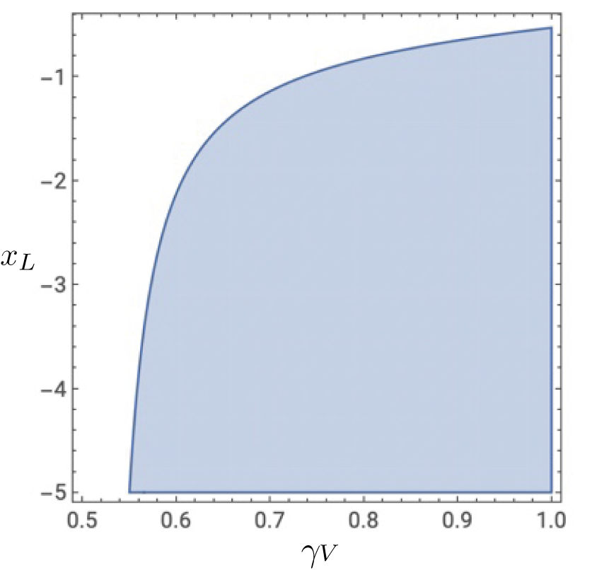
Figure 4. Gambling and Initial Disadvantage
Note: The shaded region identifies the parameter region in which gambling equilibria exist.
Having established conditions under which gambling can emerge, Propositions 2 and 3 identify the range of platforms that can be sustained in a gambling equilibrium.
Proposition 2.
There exists a unique $ {x}_L^{Min}\left(\overline{\alpha},{\gamma}_V,{x}_L\right)\ge \hskip0.35em 2\overline{\alpha}\left(2{\gamma}_V-1\right)-{x}_L^{pos} $
such that any pair of platforms that satisfies the following two properties can be sustained in a gambling equilibrium:
$ {x}_L^{Min}\left(\overline{\alpha},{\gamma}_V,{x}_L\right)\ge \hskip0.35em 2\overline{\alpha}\left(2{\gamma}_V-1\right)-{x}_L^{pos} $
such that any pair of platforms that satisfies the following two properties can be sustained in a gambling equilibrium:
-
1. The platforms are symmetric around the voter (
$ {x}_1^{R^{\ast }}-\overline{\alpha}\left(2{\gamma}_V-1\right)\hskip0.35em =\hskip0.35em \overline{\alpha}\left(2{\gamma}_V-1\right)-{x}_1^{L^{\ast }} $
). -
2. The left-wing platform is (weakly) to the right of
$ {x}_L^{Min} $
(
$ {x}_1^{L^{\ast }}\hskip0.35em \ge \hskip0.35em {x}_L^{Min} $
).


Notice that in these symmetric gambling equilibria the voter must be breaking indifference in favor of the popular party $ R $
. With any other indifference-breaking rule,
$ R $
. With any other indifference-breaking rule, $ R $
has a profitable deviation to move slightly closer to the voter and win for sure. Thus, the unpopular party chooses to lose the election with probability one, even if an arbitrarily small deviation would guarantee victory.
$ R $
has a profitable deviation to move slightly closer to the voter and win for sure. Thus, the unpopular party chooses to lose the election with probability one, even if an arbitrarily small deviation would guarantee victory.
Next, Proposition 3 shows that (under some conditions) there also exist asymmetric gambling equilibria in which the unpopular party’s platform is more extreme than his opponent’s (i.e., farther from the voter).
Proposition 3.
There exists a unique $ {x}_L^{Asym} $
such that if and only if
$ {x}_L^{Asym} $
such that if and only if $ {x}_L<{x}_L^{Asym} $
, then any pair of platforms satisfying the following two properties can also be sustained in a gambling equilibrium:
$ {x}_L<{x}_L^{Asym} $
, then any pair of platforms satisfying the following two properties can also be sustained in a gambling equilibrium:
-
1. The right-wing party commits to its global optimum (
$ {x}_1^{R^{\ast }}\hskip0.35em =\hskip0.35em {x}_R^m $
). -
2. The left-wing party is strictly farther from the voter (
$ {x}_1^{L^{\ast }}<2\overline{\alpha}\left(2{\gamma}_V-1\right)-{x}_R^m $
).


Two things are worth noticing. First, asymmetric equilibria emerge only when the unpopular party is sufficiently extreme. Second, in any asymmetric equilibrium, the popular party wins by proposing exactly the policy that maximizes its global utility ( $ {x}_R^m $
). This highlights that ideological extremism does not necessarily induce fierce opposition or divergence of interests between the parties. Quite the opposite:
$ {x}_R^m $
). This highlights that ideological extremism does not necessarily induce fierce opposition or divergence of interests between the parties. Quite the opposite:
Corollary 1. Both parties’ expected utility in any asymmetric equilibrium is (weakly) higher than in all symmetric equilibria.
Notice that in one such asymmetric equilibrium (which always exists under $ {x}_L<{x}_L^{Asym} $
), both parties propose their global optimum (i.e.,
$ {x}_L<{x}_L^{Asym} $
), both parties propose their global optimum (i.e., $ {x}_1^{R^{\ast }}\hskip0.35em =\hskip0.35em {x}_R^m $
and
$ {x}_1^{R^{\ast }}\hskip0.35em =\hskip0.35em {x}_R^m $
and $ {x}_1^{L^{\ast }}\hskip0.35em =\hskip0.35em {x}_L^m $
).Footnote
12 Intuitively, this equilibrium represents (when it exists) a natural focal point of the game on which we may expect parties to coordinate.
$ {x}_1^{L^{\ast }}\hskip0.35em =\hskip0.35em {x}_L^m $
).Footnote
12 Intuitively, this equilibrium represents (when it exists) a natural focal point of the game on which we may expect parties to coordinate.
Robustness and Alternative Assumptions
Degenerate Priors
So far, I have assumed that both parties are almost certain that the state of the world is in line with their own policy preferences (i.e., $ {\gamma}_R\hskip0.35em =\hskip0.35em 1-{\gamma}_L\hskip0.35em =\hskip0.35em 1-\varepsilon $
, where
$ {\gamma}_R\hskip0.35em =\hskip0.35em 1-{\gamma}_L\hskip0.35em =\hskip0.35em 1-\varepsilon $
, where $ \varepsilon $
is arbitrarily small). Although this stark assumption is not necessary to sustain the results, heterogeneous priors are a crucial part of the story: gambling equilibria require both parties to be sufficiently ideological in their beliefs (see Appendix B). Intuitively, the unpopular party is not willing to lose the first-period election unless it is sufficiently confident that the gamble will succeed (i.e., that the true state aligns with its own preferences). It is less straightforward to understand why the popular right-wing party may have a profitable deviation. After all, in a gambling equilibrium the party wins for sure, running on a right-wing platform. However, the popular party has a lot to lose from facilitating voter learning. If
$ \varepsilon $
is arbitrarily small). Although this stark assumption is not necessary to sustain the results, heterogeneous priors are a crucial part of the story: gambling equilibria require both parties to be sufficiently ideological in their beliefs (see Appendix B). Intuitively, the unpopular party is not willing to lose the first-period election unless it is sufficiently confident that the gamble will succeed (i.e., that the true state aligns with its own preferences). It is less straightforward to understand why the popular right-wing party may have a profitable deviation. After all, in a gambling equilibrium the party wins for sure, running on a right-wing platform. However, the popular party has a lot to lose from facilitating voter learning. If $ {\gamma}_R $
is too low, the popular party is afraid that learning will move the voter preferences to the left. The party then has an incentive to prevent information generation, and the gambling equilibria collapse. Interestingly, this implies that gambling equilibria can be sustained when the voter and the popular party share the same beliefs. However, a disagreement between the voter and the unpopular party is always necessary. Finally, I show that ideological beliefs and extreme policy preferences are, to a certain extent, substitutes. As the parties become more ideological in their beliefs, gambling equilibria can be sustained under more moderate policy preferences (Figure 5).
$ {\gamma}_R $
is too low, the popular party is afraid that learning will move the voter preferences to the left. The party then has an incentive to prevent information generation, and the gambling equilibria collapse. Interestingly, this implies that gambling equilibria can be sustained when the voter and the popular party share the same beliefs. However, a disagreement between the voter and the unpopular party is always necessary. Finally, I show that ideological beliefs and extreme policy preferences are, to a certain extent, substitutes. As the parties become more ideological in their beliefs, gambling equilibria can be sustained under more moderate policy preferences (Figure 5).

Figure 5. Gambling Equilibria under More Moderate Policy Preferences
Note: The shaded region identifies the parameter region in which gambling equilibria exist.
Purely Policy-Motivated Parties
To simplify the presentation, I maintain several of the main features of the standard spatial model. In particular, both parties must move simultaneously and the left-wing (right-wing) party can credibly commit even to radical right-wing (left-wing) platforms. These assumptions are restrictive, but they usually do not affect equilibrium results. Not so much in this model. Indeed, if we introduce office rents in the current setup, gambling equilibria can never be sustained. However, if we relax either of these assumptions (simultaneous moves or full commitment ability), gambling equilibria survive even if parties care about office as well as policy. Suppose for example that parties have full commitment ability but can choose the timing of their platform announcement. Then, gambling equilibria survive as long as office rents are not too large. This is because each party’s policy utility in a gambling equilibrium exceeds that under full convergence. Alternatively, we could assume that the parties move simultaneously but have limited commitment ability. Budge’s “New Spatial Theory” (Reference Budge1994) highlights the role of ideological consistency as a constraint, with parties only able to move within a subset of the policy space. Similarly, Levy (Reference Levy2004) argues that parties can only commit to policies in the Pareto set of their members (see also Krasa and Polborn Reference Krasa and Polborn2018). Under such limited commitment assumptions, gambling equilibria survive for sufficiently low office rents as long as the right-most (left-most) platform that the left-wing (right-wing) party can promise is not too radical. Importantly, this is true even if both parties can commit to the voter’s (expected) ideal policy.
Electoral Volatility
In the baseline model, learning about the state of the world is the only source of electoral volatility across periods. Suppose instead that, from one period to the next, voters’ preferences may also be subject to an ideological shock. Would this make gambling equilibria easier or harder to sustain? Interestingly, the answer depends on the shock’s expected direction (see Appendix B). Suppose that, in expectation, the shock will move the voter’s future preferences to the right. Then, the unpopular left-wing party’s gain from changing the voter’s beliefs increases in the expected magnitude of the shock (due to concave utility). Thus, gambling equilibria are easier to sustain the larger the average shock. The opposite holds if the shock is expected to move the voter’s future preferences to the left. Notice that these findings align with Corollary 1, despite the underlying mechanism being very different. Taken together, these results imply that an increase in the voter’s initial bias against the unpopular party (whether via beliefs about policy consequences or an ideological shock) increases the likelihood of gambling emerging in equilibrium.
Two Periods
The baseline model describes a two-period game. In Appendix B, I analyze an extension of the model where the game repeats for infinitely many periods. I show that the strategic incentives arising here mirror the two-period game, and gambling equilibria survive if (and only if) the unpopular party is sufficiently patient and extreme. In such equilibria, the unpopular party continues to gamble until the voter learns the true state of the world. Once an informative outcome is observed, the parties converge on the voter’s preferred policy in every period. Interestingly, if the unpopular party is arbitrarily patient, gambling equilibria are easier to sustain than in the two-period baseline.
Parties’ Response to Losses
How should we think about parties’ postelection behavior within the framework of this model? If a party chooses to lose an election, then why would it oust the leader, reorganize, or change its platform position following such a loss? In principle, both changing course and sticking to the status quo can be consistent with the party rationally expecting to lose. To see this, consider the infinite-horizon version of the model. At $ t\hskip0.35em =\hskip0.35em 1, $
the unpopular party gambles on the future, rationally and willingly losing the election. Depending on the voter’s payoff realization, one of two outcomes may occur. First, the voter may observe an uninformative payoff realization: no learning occurs, and the voter maintains her prior beliefs and preferences. In this case, the game remains in the gambling phase: the parties adopt the same set of platforms again at
$ t\hskip0.35em =\hskip0.35em 1, $
the unpopular party gambles on the future, rationally and willingly losing the election. Depending on the voter’s payoff realization, one of two outcomes may occur. First, the voter may observe an uninformative payoff realization: no learning occurs, and the voter maintains her prior beliefs and preferences. In this case, the game remains in the gambling phase: the parties adopt the same set of platforms again at $ t\hskip0.35em =\hskip0.35em 2 $
, with the unpopular one again choosing to lose for sure. In this scenario, no realignment or reorganization has to occur and we may expect the losing party to confirm the former leadership. Second, the voter may observe an informative payoff realization and thus discover the location of her ideal policy. The game moves to a convergence phase in period 2, and we observe platform convergence on the voter’s true optimum in every period thereafter. Suppose that the voter learns that her optimal policy is misaligned with the unpopular party: the gamble has failed, moving the voter away from the party’s own bliss point. In this case, the losing party needs to change course. We may therefore expect it to replace the former leader with a new one, willing and able to adopt positions appealing to the voter’s newly discovered preferences. If instead the gamble succeeds, the party may choose to confirm the old leadership or opt to replace it with an ideologically aligned but even more extreme one. Thus, the party’s response to electoral loss depends on the magnitude and sign of the shift in voter’s preferences across periods.
$ t\hskip0.35em =\hskip0.35em 2 $
, with the unpopular one again choosing to lose for sure. In this scenario, no realignment or reorganization has to occur and we may expect the losing party to confirm the former leadership. Second, the voter may observe an informative payoff realization and thus discover the location of her ideal policy. The game moves to a convergence phase in period 2, and we observe platform convergence on the voter’s true optimum in every period thereafter. Suppose that the voter learns that her optimal policy is misaligned with the unpopular party: the gamble has failed, moving the voter away from the party’s own bliss point. In this case, the losing party needs to change course. We may therefore expect it to replace the former leader with a new one, willing and able to adopt positions appealing to the voter’s newly discovered preferences. If instead the gamble succeeds, the party may choose to confirm the old leadership or opt to replace it with an ideologically aligned but even more extreme one. Thus, the party’s response to electoral loss depends on the magnitude and sign of the shift in voter’s preferences across periods.
Empirical Implications
Having established the existence of gambling equilibria, I now delve into the theory’s empirical implications. The goal of this section is to illustrate how both data aggregated across different contexts and in-depth analysis of specific cases may be used to provide evidence in support of my theory. None of the proposed tests is perfect, but taken together they can illuminate the relevance of the model and the mechanism it uncovers to understand parties’ behavior in real-life elections.
Aggregating Data
In order to characterize the model’s implications for analyses considering aggregate data, I begin by deriving comparative statics on the parties’ platforms in a gambling equilibrium. For simplicity, I focus on symmetric equilibria (Proposition 2), but all the empirical implications hold under asymmetric ones as well.Footnote 13
Corollary 2.
-
• Suppose
$ {\gamma}_V>\frac{1}{2} $
(i.e., the left-wing party is the unpopular one). Then, the left-most platform that can be sustained in a symmetric gambling equilibrium is decreasing in
$ {\gamma}_V $
and the right-most platform is increasing in
$ {\gamma}_V $
. -
• Suppose instead that
$ {\gamma}_V<\frac{1}{2} $
(i.e., the right-wing party is the unpopular one). Then, the left-most platform that can be sustained in a symmetric gambling equilibrium is increasing in
$ {\gamma}_V $
and the right-most platform is decreasing in
$ {\gamma}_V $
.


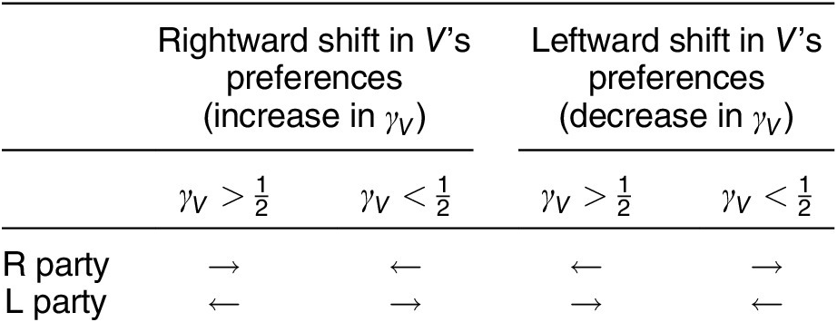
To understand this result, suppose that $ {\gamma}_V>\frac{1}{2} $
. As the voter’s initial preferences move rightward (i.e.,
$ {\gamma}_V>\frac{1}{2} $
. As the voter’s initial preferences move rightward (i.e., $ {\gamma}_V $
increases), the unpopular left-wing party has more to gain and less to lose from taking a gamble. Thus, the party is willing to allow its opponent to win with an even more extreme (and radical) right-wing platform, which further increases the amount of voter learning. In order to do so, the unpopular party must be willing to move further to the left, away from the voter. The opposite holds if
$ {\gamma}_V $
increases), the unpopular left-wing party has more to gain and less to lose from taking a gamble. Thus, the party is willing to allow its opponent to win with an even more extreme (and radical) right-wing platform, which further increases the amount of voter learning. In order to do so, the unpopular party must be willing to move further to the left, away from the voter. The opposite holds if $ {\gamma}_V $
decreases: the voter moves to the left, reducing the left-wing party’s disadvantage. This unpopular party thus has lower incentives to gamble, and its platform shifts to the right. Thus, under
$ {\gamma}_V $
decreases: the voter moves to the left, reducing the left-wing party’s disadvantage. This unpopular party thus has lower incentives to gamble, and its platform shifts to the right. Thus, under $ {\gamma}_V>\frac{1}{2} $
, the left-most platform emerging in a gambling equilibrium is always decreasing in
$ {\gamma}_V>\frac{1}{2} $
, the left-most platform emerging in a gambling equilibrium is always decreasing in $ {\gamma}_V $
. A symmetric reasoning applies to the right-wing party when
$ {\gamma}_V $
. A symmetric reasoning applies to the right-wing party when $ {\gamma}_V<\frac{1}{2} $
(see Table 1). Thus Corollary 2 shows that, in a gambling equilibrium, the unpopular party may respond to shifts in the voter’s preferences by moving in the opposite direction.
Footnote
14
$ {\gamma}_V<\frac{1}{2} $
(see Table 1). Thus Corollary 2 shows that, in a gambling equilibrium, the unpopular party may respond to shifts in the voter’s preferences by moving in the opposite direction.
Footnote
14
Table 1. Responses to Shift in Voter’s Preferences (Change in $ {\gamma}_V $
), Gambling Equilibrium
$ {\gamma}_V $
), Gambling Equilibrium
This result emphasizes that the nature of electoral competition in this model is distinct from the dynamics typically emerging in spatial elections. Probabilistic voting modelsFootnote 15 analyze an analogous trade-off, whereby policy-motivated parties may adopt a platform that decreases their probability of winning (although they would never accept to lose for sure; Calvert Reference Calvert1985; Wittman Reference Wittman1983). Yet, the parties’ (instrumental) desire to win still drives electoral competition. Thus, both equilibrium platforms always move in the same direction as the (expected) median voter. Other theories hypothesize that parties are constrained in this adaptation process, but they nonetheless predict that if parties move at all, they follow the electorate (e.g., Dalton and McAllister Reference Dalton and McAllister2015).
Thus, Corollary 2 suggests that the model’s predictions may differ starkly from those of competing theories. But how do we translate the theoretical results from this corollary into implications for analyses considering aggregate data? In answering this question, one important caveat must be considered. Corollary 2 describes comparative statics that hold in a gambling equilibrium. However, when the conditions in Proposition 1 fail, the equilibrium takes the familiar form of Downsian convergence. Furthermore, gambling equilibria are not unique: an additional equilibrium in convergence always exists. Finally, platform convegrgence always occurs in the second period of the two-period model (and in any period following an informative outcome realization in the infinite-horizon model). Thus, even if my model correctly describes the data-generating process and gambling behavior emerges in real life, we may observe a mix of equilibria (i.e., gambling and convergence) when we aggregate data across different contexts or periods. Any statement about the theory’s implications in the aggregate must therefore be a statement about average effects, where the average is across different equilibria.
Keeping this in mind, we can derive the first observable implication of the theory if we compare how popular and unpopular parties respond to shifts in the electorate:
Implication 1. Consider the following regression:
 $$ \hskip-0.5em Pla{t}_{it}\hskip0.35em =\hskip0.35em \alpha +{\beta}_1{V}_t+{\beta}_2 Unpo{p}_{it}+{\beta}_3{V}_t\times Unpo{p}_{it}+{\varepsilon}_{it}, $$
where $ {Plat}_{it} $
is the left–right position of party i’s platform at time t, Vt is the position of the (median) voter at time t, and
$ {Plat}_{it} $
is the left–right position of party i’s platform at time t, Vt is the position of the (median) voter at time t, and $ {Unpop}_{it} $
is a binary indicator taking value one if party i at time t is unpopular and zero otherwise. Then,
$ {Unpop}_{it} $
is a binary indicator taking value one if party i at time t is unpopular and zero otherwise. Then, $ {\beta}_3 $
should have a negative sign.
$ {\beta}_3 $
should have a negative sign.
As discussed above, even if the novel gambling equilibria identified in my theory emerge in real life, when considering aggregate data researchers will obtain a mix of both gambling and convergence. To illustrate how this influences our expectations over the sign of the coefficients in Equation 3, Table 2 considers a thought experiment (each cell describes the expected effect of a one-unit increase—a rightward shift—in the voter’s ex ante preferred policy). First, suppose all the observations in the dataset feature parties playing a convergence equilibrium. Then, because in such equilibrium both parties always move in the same direction as the electorate (and by exactly the same amount), we should obtain $ {\beta}_1>0 $
and
$ {\beta}_1>0 $
and $ {\beta}_3\hskip0.35em =\hskip0.35em 0 $
. Suppose instead all observations are drawn from gambling equilibria. Corollary 2 indicates that, in this case, the popular party will move in the same direction as the voter; therefore,
$ {\beta}_3\hskip0.35em =\hskip0.35em 0 $
. Suppose instead all observations are drawn from gambling equilibria. Corollary 2 indicates that, in this case, the popular party will move in the same direction as the voter; therefore, $ {\beta}_1>0 $
. In contrast, the unpopular one will move in the opposite direction. Thus, we should obtain
$ {\beta}_1>0 $
. In contrast, the unpopular one will move in the opposite direction. Thus, we should obtain $ {\beta}_1+{\beta}_3<0 $
(which implies
$ {\beta}_1+{\beta}_3<0 $
(which implies $ {\beta}_3<0 $
). Therefore,
$ {\beta}_3<0 $
). Therefore, $ {\beta}_3 $
will be equal to 0 in a convergence equilibrium and take negative value in a gambling one. Notice that this holds regardless of whether
$ {\beta}_3 $
will be equal to 0 in a convergence equilibrium and take negative value in a gambling one. Notice that this holds regardless of whether $ {\gamma}_V>\frac{1}{2} $
or
$ {\gamma}_V>\frac{1}{2} $
or $ {\gamma}_V<\frac{1}{2} $
(i.e., of the identity of the unpopular party).
$ {\gamma}_V<\frac{1}{2} $
(i.e., of the identity of the unpopular party).
Table 2. Parties’ Response to One-Unit Rightward Shift in Voter’s Preferences
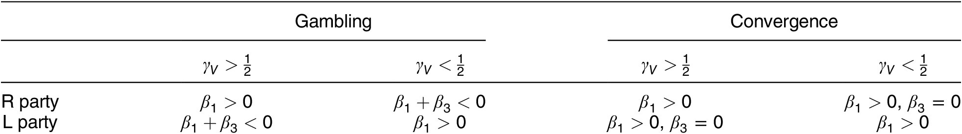
Substantively, this has two consequences for what researchers should observe when considering aggregate data. First, the model does not discipline our (absolute) directional expectations on how unpopular parties respond to shifts in voters’ preferences. In a convergence equilibrium, the unpopular party moves with the voter. In a gambling one, it moves in the opposite direction. Thus, $ {\beta}_1+{\beta}_3 $
may have, on average, a positive or a negative sign (or even be a zero). Second, and most importantly, the prediction on how unpopular parties respond relative to popular ones is instead well defined. Because in a convergence equilibrium both parties move in the same direction, and by the same amount, the sign of
$ {\beta}_1+{\beta}_3 $
may have, on average, a positive or a negative sign (or even be a zero). Second, and most importantly, the prediction on how unpopular parties respond relative to popular ones is instead well defined. Because in a convergence equilibrium both parties move in the same direction, and by the same amount, the sign of $ {\beta}_3 $
will only capture the platform shifts occurring in gambling equilibria. Thus, when aggregating across equilibria (and if a gambling equilibrium obtains in some place at some time), we should obtain
$ {\beta}_3 $
will only capture the platform shifts occurring in gambling equilibria. Thus, when aggregating across equilibria (and if a gambling equilibrium obtains in some place at some time), we should obtain $ {\beta}_3<0 $
.
$ {\beta}_3<0 $
.
The specific analysis described in Implication 1 has yet to be conducted. However, several scholars have uncovered evidence of parties responding to shifts in the electorate by moving in the opposite direction, in sharp contrast with the predictions of the pure spatial theory of elections (see, e.g., Adams, Haupt, and Stoll Reference Adams, Haupt and Stoll2009; Schumacher, de Vries, and Vis Reference Schumacher, de Vries and Vis2013). The research design proposed above allows researchers to delve deeper into these results and investigate whether my theory may help explain these surprising patterns.
One potential challenge is that evaluating the party-level prediction detailed in Implication 1 requires a measure of party popularity. Focusing on the theory’s implications at the election level may provide a more promising avenue for empirical analysis:Footnote 16
Implication 2. As the voter’s ex ante preferences become more radical, platform polarization should increase on average.
This follows directly from Corollary 2. Notice that, when $ {\gamma}_V>\frac{1}{2} $
, the voter’s preferences become more radical (i.e., move away from zero) as
$ {\gamma}_V>\frac{1}{2} $
, the voter’s preferences become more radical (i.e., move away from zero) as $ {\gamma}_V $
increases. In contrast, if
$ {\gamma}_V $
increases. In contrast, if $ {\gamma}_V<\frac{1}{2} $
, voter radicalism increases as
$ {\gamma}_V<\frac{1}{2} $
, voter radicalism increases as $ {\gamma}_V $
decreases. Then, in a gambling equilibrium the parties’ platforms move away from each other as
$ {\gamma}_V $
decreases. Then, in a gambling equilibrium the parties’ platforms move away from each other as $ {\gamma}_V $
moves away from
$ {\gamma}_V $
moves away from $ \frac{1}{2} $
(see Table 1). Recall that platform polarization is instead constant in a convergence equilibrium. Therefore, the sign of the average effect (across equilibria) is again unambiguous: the maximum amount of platform polarization sustainable in equilibrium increases as the voter becomes more radical. To the best of my knowledge, no empirical work has investigated the link between voter radicalism and platform polarization. Indeed, Curini and Hino (Reference Curini and Hino2012) lament the literature’s almost exclusive focus on the institutional determinants of platform polarization. Thus, this is a promising avenue for future research.
$ \frac{1}{2} $
(see Table 1). Recall that platform polarization is instead constant in a convergence equilibrium. Therefore, the sign of the average effect (across equilibria) is again unambiguous: the maximum amount of platform polarization sustainable in equilibrium increases as the voter becomes more radical. To the best of my knowledge, no empirical work has investigated the link between voter radicalism and platform polarization. Indeed, Curini and Hino (Reference Curini and Hino2012) lament the literature’s almost exclusive focus on the institutional determinants of platform polarization. Thus, this is a promising avenue for future research.
Finally, consider the theory’s implications for the observed electoral consequences of parties’ strategic positioning. Suppose that scholars compare two sets of elections: one where the parties are playing a gambling equilibrium and therefore selecting more extreme platforms and another where the parties are converging on the voter’s preferences. Recall that in a convergence equilibrium both parties win with positive probability. Conversely, in any gambling equilibrium the popular party wins with probability one. Implication 3 follows:
Implication 3. On average, popular parties should perform better in the elections in which they select a more extreme platform. In contrast, the opposite holds for unpopular parties.
Empirical scholars have often emphasized a surprising lack of consistent findings on the electoral consequences of parties’ platform positioning. For example, Adams et al. (Reference Adams, Clark, Ezrow and Glasgow2006) conclude that mainstream parties don’t perform better (or worse) on average when they moderate their platforms in the direction of the electorate. Implication 3 indicates that this null result may emerge from averaging across coefficients with different signs: positive for unpopular parties and negative for popular ones.
In concluding this section, a qualification is in order. Implications 1–3 indicate that the theory can generate clear directional predictions about average effects. However, as discussed above, the multiplicity of equilibria and the periods of convergence following successful gambling imply that estimates would be diluted toward zero (compared with the expected effects if we could isolate gambling equilibria) and the associated standard errors would be inflated. In addition, Implications 1 and 3 refer to interaction effects, which tend to be harder to detect (statistically) than are their constituent effects. This concern is especially relevant because the proposed analyses consider outcomes at the election (or election-party) level; therefore, the sample size is bounded above by the number of races. Thus, even if gambling equilibria do emerge as posited in real life, the conditions under which empirical researchers would recover statistically significant estimates, enabling them to disentangle signal from noise, are demanding.
Delving into Specific Cases
The tests proposed in the previous section can help us appreciate the theory’s implications when we consider average effects across many cases. However, even beyond the caveats discussed above, such tests would not provide direct evidence that my mechanism is at play in any one case. Therefore, I briefly illustrate how in-depth examination of individual cases may help establish that all the pieces of the theory hold together in the mechanism I propose (Beach and Pedersen Reference Beach and Pedersen2019). To do this, I briefly revisit the Goldwater motivating example through the lenses of the model. Thus, the purpose of this section is twofold: presenting some preliminary evidence that my mechanism may underlie the Goldwater phenomenon while also providing a useful road map that future research may follow when assessing the relevance of the theory in this and other cases.
Barry Goldwater espoused an extreme right-wing platform during the 1964 presidential campaign and went on to suffer a burning but widely anticipated defeat. According to my theory, Goldwater gambled on the future: he knowingly adopted an electorally unviable position in hopes of changing the voters’ future preferences.
The first component of the theory is that this behavior may only emerge when parties are forward-looking and thus look beyond winning the upcoming elections when deciding their optimal strategy. Indeed, historians and political commentators alike maintain that Goldwater’s 1964 strategy was directed at “a higher goal than president of the United States” (Volle Reference Volle2010, 45). His “was a radical plan, not calculated to win … but to challenge the minds and hearts of voters and produce a Conservative wave in America” (Edwards Reference Edwards2014, 8).
Furthermore, only an unpopular party may exhibit gambling behavior in equilibrium. Looking at public opinion in the lead-up to the 1964 election, we observe evidence aligning with this. The election in fact took place within the context of the so-called Liberal Consensus in American politics (see, e.g., Perlstein Reference Perlstein2009, xi). This is also reflected in the parties’ strategies in the elections immediately preceding the 1964 race: both parties adopted relatively liberal platforms, shifting further leftward between 1956 and 1960, precisely as we would expect under the classic spatial logic (see Figure 6).Footnote 17

Figure 6. Right–Left Positioning (RILE score, Comparative Manifesto Project) of Republican and Democratic Platforms
Instead, if we look at the 1964 race, things appear to be very different. The Democrats continued to move to the left, whereas the Republican platform shifted significantly to the right. Following the logic of my model, Goldwater was presented with a trade-off: continue compromising and adopt an electorally viable position close to the center of the policy space (with little hopes of generating an informative outcome and changing the voter’s future preferences) or allow its opponent to win and implement a more radical platform in hopes of facilitating voter learning and obtaining a better policy in the future. Indeed, we can notice that, although Goldwater’s platform was electorally untenable (in the model’s language, too extreme), it was no more radical than his opponent’s (i.e., the two platforms are equally distant from the center of the policy space). This illustrates the source of the unpopular party’s trade-off: its popular opponent can win with relative more radical, and thus more informative, platforms. This generates incentives to gamble on the future. Moreover, in line with the theory, scholars argue that Goldwater’s gamble was induced by extreme preferences coupled with ideological beliefs: he was willing to lose because had faith that “history would prove him right” (Volle Reference Volle2010, 50).
Evidence suggests that this is one instance in which the gamble paid off. The model predicts a return to platform convergence in the second period, tilted in the direction of the unpopular party in case of a successful gamble (i.e., if the voter learns that her optimal policy is aligned with the party’s). This is precisely what we observe in the 1968 elections. The Republican and Democratic platforms converged toward each other, both moving significantly to the right compared with the 1960 campaign.Footnote 18 This suggests that Goldwater’s strategy successfully moved the center of the electoral space to the right. Indeed, Stimson’s (Reference Stimson1999) Policy Mood Index shows a rightward shift in the electorate between 1964 and 1968.Footnote 19 This shift, scholars argue, would prove to be long-lasting: Goldwater’s gamble is often credited for paving the way for Reagan’s election (Will Reference Will1998) making this “one time, at least, in which history was written by the losers” (Perlstein Reference Perlstein2009, x).
Conclusion
The contribution of this paper is to demonstrate that behavior typically considered as expressive, and thus explained “in its own terms” rather than “in terms of preferences over outcomes” (Brennan and Buchanan Reference Brennan and Buchanan1984, 187), may instead arise from strategic considerations coupled with fundamental behavioral tendencies, such as heterogeneous prior beliefs. Although this project has focused on political parties’ strategic platform positioning, its main insights may extend beyond this specific context.
Pons and Tricaud (Reference Pons and Tricaud2018) analyze run-off elections in France to investigate how the presence of third candidates influences electoral outcomes. They show that third entrants often end up hurting their own ideological camp, as “in 19.2 percent of the elections, the presence of the third candidate causes the loss of the candidate among the top two that is ideologically closest to her” (1623). As the authors themselves argue, these results are “difficult to rationalize … in particular when the third candidate appears to have slim chances of being a front-runner in the second round” (1623). My theory suggests a mechanism under which concerns for future policy, combined with ideological beliefs over possible policy consequences, may generate this type of behavior. Moreover, the model provides a framework for understanding under which conditions such behavior is more or less likely to emerge.
Similar dynamics may be at play in the context of legislative bargaining. Bargaining players sometimes appear unwilling to compromise, and this rigidity is typically interpreted as a desire to maintain their ideological purity (Mann and Ornstein Reference Mann and Ornstein2016). My theory suggests an alternative rationale. Forward-looking actors may accept a worse policy today if they are convinced that the resulting outcome will alter the electorate’s beliefs in a way that provides them a stronger bargaining position in the future. Consider for example the bargaining between the U.S. Congress and President Donald Trump over the repeal of Obamacare. Soon after the Republican bill to repeal the Affordable Care Act was pulled from the House for insufficient support, Trump adopted the strategy of keeping the status quo rather than looking for a compromise. “The best thing politically is let Obamacare explode,” Trump argued. The logic behind this strategy seems to align with the mechanism advocated in this paper: Trump believed that keeping the policy in place would show American voters the flaws of the current system and thus generate stronger support for a reform (Bryan Reference Bryan2017).
A relatively small and well-defined deviation from Bayesian rationality—namely, the noncommon priors assumption—potentially allows us to shed new light on the strategic considerations underlying several phenomena usually ascribed to expressive motivations.
Supplementary Materials
To view supplementary material for this article, please visit http://doi.org/10.1017/S0003055422000843.
DATA AVAILABILITY STATEMENT
Replication files for this study are available at the American Political Science Review Dataverse: https://doi.org/10.7910/DVN/RQNVFW.
ACKNOWLEDGMENTS
I am grateful to Torun Dewan, Selina Hofstetter, Giovanna Invernizzi, Michael Joseph, Gleason Judd, Korhan Koçak, Clement Minaudier, Salvatore Nunnari, Branislav Slantchev, Arduino Tomasi, and Stephane Wolton for helpful comments and suggestions.
CONFLICT OF INTEREST
The author declares no ethical issues or conflicts of interest in this research.
ETHICAL STANDARDS
The author affirms this research did not involve human subjects.


 Open access
Comments
No Comments have been published for this article.