


1. Introduction
Flapping wings or tails are frequently employed in the locomotion of aerial and aquatic animals (Wang Reference Wang2005; Wu Reference Wu2011; Liu, Wang & Liu Reference Liu, Wang and Liu2024). On the one hand, this is because biological systems do not support rotor-like spinning machines. On the other hand, the flapping wing has more aerodynamic or hydrodynamic advantages at moderate Reynolds numbers, such as high lift, low noise and agility (Lighthill Reference Lighthill1969; Eldredge & Jones Reference Eldredge and Jones2019; Jaworski & Peake Reference Jaworski and Peake2020). Over billions of years of evolution, animals have adapted to various environments and developed highly efficient locomotion capabilities. Studying the dynamic and biological mechanisms underlying these abilities serves as a rich source of inspiration for bio-inspired design.
The rigid plate with prescribed pitching and heaving motion has been widely used in the modelling of the animal wing due to its simplicity and close relevance to most biological systems (Triantafyllou, Triantafyllou & Gopalkrishnan Reference Triantafyllou, Triantafyllou and Gopalkrishnan1991; Anderson et al. Reference Anderson, Streitlien, Barrett and Triantafyllou1998; Dong, Mittal & Najjar Reference Dong, Mittal and Najjar2006; Green, Rowley & Smits Reference Green, Rowley and Smits2011; Ayancik et al. Reference Ayancik, Zhong, Quinn, Brandes, Bart-Smith and Moored2019; Zhu, Mathai & Breuer Reference Zhu, Mathai and Breuer2021; Chao, Jia & Li Reference Chao, Jia and Li2024; Jin et al. Reference Jin, Wang, Ravi, Young, Lai and Tian2024). For instance, von Ellenrieder, Parker & Soria (Reference von Ellenrieder, Parker and Soria2003) visualised the three-dimensional flow structures behind a heaving and pitching finite-span wing and showed that variations in Strouhal number, pitch amplitude and phase angle can significantly alter the wake topology. Buchholz & Smits (Reference Buchholz and Smits2006) examined the wake of a low-aspect-ratio pitching panel and identified alternating horseshoe vortices whose streamwise legs dominate the wake dynamics at small aspect ratios. Later, Buchholz & Smits (Reference Buchholz and Smits2008) experimentally quantified the thrust generation of a finite-aspect-ratio panel pitching about its leading edge, showing that the thrust coefficient increases monotonically with the Strouhal number, aspect ratio and Reynolds number. In a related but distinct study, Quinn et al. (Reference Quinn, Moored, Dewey and Smits2014) investigated unsteady propulsion of a pitching foil near a solid boundary and demonstrated that ground effect can enhance thrust by up to $40\,\%$
at the equilibrium position where the time-averaged lift is zero. Regarding the development of a generic scaling analysis for flapping foils, Floryan et al. (Reference Floryan, Van Buren, Rowley and Smits2017) presented scaling relations for the thrust coefficient, power coefficient and propulsive efficiency of rigid foils undergoing either heaving or pitching motions, considering unsteady lift and added mass forces. They demonstrated that the mean thrust for heaving is entirely lift based, while for pitching, it is solely due to added mass. However, the mean input power and propulsive efficiency depend on contributions from both mechanisms. These scaling laws were validated through water tunnel experiments on a nominally two-dimensional flapping plate in a free stream, as well as by biological data of swimming aquatic animals. In a related study, Van Buren, Floryan & Smits (Reference Van Buren, Floryan and Smits2019) experimentally investigated rigid foils undergoing combined heaving and pitching motions in a free stream, considering the effect of phase difference. Their findings revealed that the pitching motion should lag the heaving motion by approximately
$40\,\%$
at the equilibrium position where the time-averaged lift is zero. Regarding the development of a generic scaling analysis for flapping foils, Floryan et al. (Reference Floryan, Van Buren, Rowley and Smits2017) presented scaling relations for the thrust coefficient, power coefficient and propulsive efficiency of rigid foils undergoing either heaving or pitching motions, considering unsteady lift and added mass forces. They demonstrated that the mean thrust for heaving is entirely lift based, while for pitching, it is solely due to added mass. However, the mean input power and propulsive efficiency depend on contributions from both mechanisms. These scaling laws were validated through water tunnel experiments on a nominally two-dimensional flapping plate in a free stream, as well as by biological data of swimming aquatic animals. In a related study, Van Buren, Floryan & Smits (Reference Van Buren, Floryan and Smits2019) experimentally investigated rigid foils undergoing combined heaving and pitching motions in a free stream, considering the effect of phase difference. Their findings revealed that the pitching motion should lag the heaving motion by approximately $30^\circ$
to maximise thrust and by approximately
$30^\circ$
to maximise thrust and by approximately $90^\circ$
to maximise the propulsive efficiency. Expanding on the scaling law developed by Floryan et al. (Reference Floryan, Van Buren, Rowley and Smits2017) for individual heaving or pitching motions, Van Buren et al. (Reference Van Buren, Floryan and Smits2019) developed new scaling laws for combined heaving and pitching motions, considering the phase offset between them, which were validated by experimental data.
$90^\circ$
to maximise the propulsive efficiency. Expanding on the scaling law developed by Floryan et al. (Reference Floryan, Van Buren, Rowley and Smits2017) for individual heaving or pitching motions, Van Buren et al. (Reference Van Buren, Floryan and Smits2019) developed new scaling laws for combined heaving and pitching motions, considering the phase offset between them, which were validated by experimental data.
Inspired by the role of flexibility in aerial locomotion, particularly in structures such as flying animals’ wings (Wootton Reference Wootton1992; Brodsky Reference Brodsky1994), researchers have studied passive or active deformation, in addition to passive flapping (Spagnolie et al. Reference Spagnolie, Moret, Shelley and Zhang2010; Zhang, Liu & Lu Reference Zhang, Liu and Lu2010), to gain deeper insights into how structural flexibility influences locomotor performance (Liao et al. Reference Liao, Beal, Lauder and Triantafyllou2003; Shyy et al. Reference Shyy, Aono, Chimakurthi, Trizila, Kang, Cesnik and Liu2010; Zhu, He & Zhang Reference Zhu, He and Zhang2014a , Reference Zhu, He and Zhangb ; Gazzola, Argentina & Mahadevan Reference Gazzola, Argentina and Mahadevan2015; Hoover et al. Reference Hoover, Cortez, Tytell and Fauci2018; Smits Reference Smits2019; Liu et al. Reference Liu, Wang and Liu2024). Experimental studies conducted by Thiria & Godoy-Diana (Reference Thiria and Godoy-Diana2010) and Ramananarivo, Godoy-Diana & Thiria (Reference Ramananarivo, Godoy-Diana and Thiria2011) investigated the self-propulsion of flexible plates in the air. They found that flapping frequencies lower than the natural frequency of the flexible plate maximise the thrust coefficient and propulsive efficiency. Their experimental observations matched well with predictions from a nonlinear oscillator model, which incorporated cubic structural nonlinearities and both linear and quadratic damping terms. The modelling further revealed that non-resonant behaviour emerges both in the presence of nonlinear damping at small flapping amplitudes and due to geometric saturation effects at large amplitudes. Therefore, resonance mechanisms cannot explain the observed performance optimum. Instead, they found that at the optimal frequency ratio, the instantaneous angle of attack and the trailing-edge deflection angle become equal at the moment of maximum flapping velocity, a configuration that is more favourable for generating aerodynamic pressure contributing to thrust. Kang et al. (Reference Kang, Aono, Cesnik and Shyy2011) numerically investigated the flapping dynamics of flexible plates. They found that the maximum propulsive force is achieved slightly below resonance. In contrast, the optimal propulsive efficiency occurs when the flapping frequency is approximately half the natural frequency. A non-dimensional tip-deformation parameter was proposed to characterise the structural response, and both the time-averaged force and efficiency were shown to scale with this parameter. Alben et al. (Reference Alben, Witt, Baker, Anderson and Lauder2012) observed resonant-like peaks in the self-propulsive speed as the length and rigidity of the flexible plate were varied, both in numerical simulations and experiments. The inviscid model predicted that the self-propulsive speed scales with the length and rigidity, and these scalings were validated by experimental data. It has also been reported that the optimal propulsive efficiency can occur below (Ramananarivo et al. Reference Ramananarivo, Godoy-Diana and Thiria2011), at (Michelin & Llewellyn Smith Reference Michelin and Llewellyn Smith2009) or above the resonant frequency (Masoud & Alexeev Reference Masoud and Alexeev2010). All of these cases were observed in the experimental study (Dewey et al. Reference Dewey, Boschitsch, Moored, Stone and Smits2013) of flexible pitching panels in free-stream flow. Therefore, there is no consensus on whether resonance plays a definitive role in maximising thrust and propulsive efficiency.
It is important to note that the above-mentioned investigations into flexible plates treat those plates as inextensible. In comparison, compliant membranes possess finite in-plane stretching, allowing them to adapt to changing flow conditions through passive deformation and elastic extension (Swartz et al. Reference Swartz, Groves, Kim and Walsh1996; Shyy, Berg & Ljungqvist Reference Shyy, Berg and Ljungqvist1999; Song et al. Reference Song, Tian, Israeli, Galvao, Bishop, Swartz and Breuer2008; Cheney et al. Reference Cheney, Konow, Bearnot and Swartz2015; Mavroyiakoumou & Alben Reference Mavroyiakoumou and Alben2020, Reference Mavroyiakoumou and Alben2022; Mathai et al. Reference Mathai, Das, Naylor and Breuer2023). Unlike rigid or purely inextensible plates, membranes with finite in-plane stretching have been demonstrated to reduce flow separation and delay stall. The aerodynamic performance improvements of such membrane wings have been reviewed by Lian et al. (Reference Lian, Shyy, Viieru and Zhang2003) and Tiomkin & Raveh (Reference Tiomkin and Raveh2021). Tiomkin and colleagues (Tiomkin & Raveh Reference Tiomkin and Raveh2017, Reference Tiomkin and Raveh2019; Tiomkin & Jaworski Reference Tiomkin and Jaworski2022) developed theoretical models that couple thin-airfoil aerodynamics with membrane elasticity to describe the unsteady response and aeroelastic stability of membrane wings. In particular, Waldman & Breuer (Reference Waldman and Breuer2017) presented a model that incorporates the Young–Laplace equation to capture the nonlinear deformation of a membrane at low angles of attack and employs thin-airfoil theory to approximate the aerodynamic pressure acting on the membrane. The predicted camber, lift and vibrational frequency show good agreement with numerical simulations and experimental observations. Furthermore, Tzezana & Breuer (Reference Tzezana and Breuer2019) developed a theoretical framework that combines thin-airfoil theory with a membrane equation to model both steady and flapping membranes. As the flapping frequency increases, the membranes transition from thrust to drag near the resonant frequency, with this transition occurring earlier for more compliant membranes. Additionally, the wake experiences a transition from a reverse von Kármán vortex street to a traditional von Kármán vortex street. For highly compliant membranes, the wake transition frequency is predicted to be higher than the thrust–to-drag transition frequency. In the domain of numerical simulations and experiments, Lauber, Weymouth & Limbert (Reference Lauber, Weymouth and Limbert2023) employs a fully coupled fluid–structure interaction approach to investigate the effects of the Strouhal number and membrane compliance on the flight performance of bat-like flapping membrane wings, specifically designed to mimic the biomechanics of the handwing. They showed that a peak in both propulsive and lift efficiencies occurs near ${\textit{St}} \approx 0.5$
, which is significantly higher than the classical optimal Strouhal number range of
${\textit{St}} \approx 0.5$
, which is significantly higher than the classical optimal Strouhal number range of ${\textit{St}} \approx 0.2$
–
${\textit{St}} \approx 0.2$
– $0.4$
reported for the locomotion of birds and fishes (Triantafyllou, Triantafyllou & Grosenbaugh Reference Triantafyllou, Triantafyllou and Grosenbaugh1993; Taylor, Nudds & Thomas Reference Taylor, Nudds and Thomas2003). This shift is attributed to the specialised kinematics of bat flight. Moreover, they also found that, while reducing membrane stiffness improves propulsive efficiency, excessive compliance induces flutter and significantly degrades performance, and introducing anisotropy into the material model helps delay the onset of flutter.
$0.4$
reported for the locomotion of birds and fishes (Triantafyllou, Triantafyllou & Grosenbaugh Reference Triantafyllou, Triantafyllou and Grosenbaugh1993; Taylor, Nudds & Thomas Reference Taylor, Nudds and Thomas2003). This shift is attributed to the specialised kinematics of bat flight. Moreover, they also found that, while reducing membrane stiffness improves propulsive efficiency, excessive compliance induces flutter and significantly degrades performance, and introducing anisotropy into the material model helps delay the onset of flutter.
In contrast, the numerical study by Kumar, Seo & Mittal (Reference Kumar, Seo and Mittal2025) incorporates both the handwing and the armwing, enabling a more complete representation of bat wing kinematics. They employ a force partitioning method to analyse the aerodynamic forces and show that the dominant contribution arises from Q-induced forces, while the time-averaged contribution of kinematic forces is minimal. Here, $Q$
is the second invariant of the velocity gradient tensor. However, the time variation of the various partitions of the pressure-induced lift and drag forces reveals that the primary source of force oscillations is the kinematic component. This insight highlights the important role of unsteady inertial effects, particularly those associated with wing flutter. Similarly, Gehrke & Mulleners (Reference Gehrke and Mulleners2025) experimentally investigated the effects of the in-plane stretching stiffness and pitching amplitude on the lift and efficiency of a flapping membrane in a stationary fluid. In their set-up, the membrane undergoes a prescribed horizontal heaving motion while maintaining a constant pitching angle throughout the flapping cycle. They identified distinct optimal values for the in-plane stretching stiffness and angle of attack, which maximise lift and efficiency, respectively. They observed different vortex patterns, and, unlike the rigid plate, it is no longer the leading-edge vortex that generates lift. Instead, the curvature of the membrane suppresses the leading-edge vortex. Vorticity then accumulates in a bound shear layer that covers the entire membrane, thereby enhancing lift.
$Q$
is the second invariant of the velocity gradient tensor. However, the time variation of the various partitions of the pressure-induced lift and drag forces reveals that the primary source of force oscillations is the kinematic component. This insight highlights the important role of unsteady inertial effects, particularly those associated with wing flutter. Similarly, Gehrke & Mulleners (Reference Gehrke and Mulleners2025) experimentally investigated the effects of the in-plane stretching stiffness and pitching amplitude on the lift and efficiency of a flapping membrane in a stationary fluid. In their set-up, the membrane undergoes a prescribed horizontal heaving motion while maintaining a constant pitching angle throughout the flapping cycle. They identified distinct optimal values for the in-plane stretching stiffness and angle of attack, which maximise lift and efficiency, respectively. They observed different vortex patterns, and, unlike the rigid plate, it is no longer the leading-edge vortex that generates lift. Instead, the curvature of the membrane suppresses the leading-edge vortex. Vorticity then accumulates in a bound shear layer that covers the entire membrane, thereby enhancing lift.
Beyond bio-inspired studies of flapping flight, compliant membranes have also been investigated for their potential in flow energy harvesting. For example, Mathai et al. (Reference Mathai, Tzezana, Das and Breuer2022) experimentally studied a flexible membrane oscillating in a uniform flow and demonstrated that it could extract up to $160\,\%$
more power than a rigid plate. This enhancement was attributed to the increased lateral force resulting from the delayed shedding of the leading-edge vortex. Similarly, Upfal et al. (Reference Upfal, Zhu, Handy-Cardenas and Breuer2025) investigated a shape-morphing membrane foil in an energy-harvesting configuration and found that, at moderately high effective angles of attack, membrane compliance stabilises the leading-edge vortex and delays dynamic stall, enhancing efficiency, whereas excessive deformation at very high angles leads to performance degradation. In a related study, Gehrke et al. (Reference Gehrke, Richeux, Uksul and Mulleners2022) examined a bio-inspired flapping membrane wing in a hovering configuration and showed that its aerodynamic performance increases with effective angle of attack up to an intermediate-to-high range, beyond which excessive angles lead to stronger flow separation and a reduction in lift. In the present work, however, we restrict our analysis to moderate-to-low effective angles of attack (approximately
$160\,\%$
more power than a rigid plate. This enhancement was attributed to the increased lateral force resulting from the delayed shedding of the leading-edge vortex. Similarly, Upfal et al. (Reference Upfal, Zhu, Handy-Cardenas and Breuer2025) investigated a shape-morphing membrane foil in an energy-harvesting configuration and found that, at moderately high effective angles of attack, membrane compliance stabilises the leading-edge vortex and delays dynamic stall, enhancing efficiency, whereas excessive deformation at very high angles leads to performance degradation. In a related study, Gehrke et al. (Reference Gehrke, Richeux, Uksul and Mulleners2022) examined a bio-inspired flapping membrane wing in a hovering configuration and showed that its aerodynamic performance increases with effective angle of attack up to an intermediate-to-high range, beyond which excessive angles lead to stronger flow separation and a reduction in lift. In the present work, however, we restrict our analysis to moderate-to-low effective angles of attack (approximately $10^\circ$
–
$10^\circ$
– $40^\circ$
), focusing on the propulsive regime rather than the high-angle flow-separation dynamics.
$40^\circ$
), focusing on the propulsive regime rather than the high-angle flow-separation dynamics.
Despite the existing theoretical, numerical and experimental works on membranes with finite in-plane stretching, fundamental physical questions remain unanswered: How does the membrane’s stretching stiffness at different levels alter the strength of vortex structures formed on the membrane and impact its dynamic performance? And how can we capture this coupled fluid–structure dynamics in a unified scaling framework that predicts thrust and power? To address these questions, we perform fully coupled fluid–structure interaction simulations of a two-dimensional membrane undergoing simultaneous heaving and pitching in a uniform flow, while systematically varying the membrane’s stretching stiffness, Strouhal number and pitching amplitude. By analysing the evolution of vortices and membrane dynamics, we uncover the physical mechanisms through which propulsion performance is enhanced and modify scaling laws that capture the dominant contributions to thrust and power, with good agreement across a wide range of parameters.
The remainder of this paper is organised as follows. The physical problem and mathematical formulation are presented in § 2.1. The numerical method is described in § 2.2. Detailed results are discussed in § 3, and concluding remarks are addressed in § 4.
2. Computational model
2.1. Physical problem and mathematical formulation
A two-dimensional model of a membrane with finite in-plane stretching flapping in uniform flow is considered. As shown in figure 1, a compliant membrane with an original length $c_0$
in the flat and stress-free state is pre-stretched to a length
$c_0$
in the flat and stress-free state is pre-stretched to a length $c$
and immersed in a viscous fluid. The computational domain is an
$c$
and immersed in a viscous fluid. The computational domain is an $L_X\times L_Y$
rectangle, where
$L_X\times L_Y$
rectangle, where $L_X$
and
$L_X$
and $L_Y$
are the domain sizes in the
$L_Y$
are the domain sizes in the $x\hbox{-}$
and
$x\hbox{-}$
and $y\hbox{-}$
directions, respectively.
$y\hbox{-}$
directions, respectively.
Schematic diagram of a membrane flapping in a uniform incoming flow. Here, $2 h_0$
denotes the peak-to-peak heaving displacement, and
$2 h_0$
denotes the peak-to-peak heaving displacement, and $\theta (t)$
represents the instantaneous pitching angle.
$\theta (t)$
represents the instantaneous pitching angle.

To investigate this system of fluid–membrane interaction, the incompressible Navier–Stokes equations are solved to simulate the flow
 \begin{align} \rho \frac {\partial \boldsymbol{v}}{\partial t}+\rho \boldsymbol{v}\boldsymbol{\cdot }\boldsymbol{\nabla }\boldsymbol{v}&=-\boldsymbol{\nabla }p+\mu \boldsymbol{\nabla} ^2\boldsymbol{v}+ \boldsymbol{f}_{\kern-1.5pt b}, \end{align}
 \begin{align} \boldsymbol{\nabla }\boldsymbol{\cdot }\boldsymbol{v}&=0, \end{align}
where $\boldsymbol{v}$
is the velocity,
$\boldsymbol{v}$
is the velocity, $p$
the pressure,
$p$
the pressure, $\rho$
the density of the fluid,
$\rho$
the density of the fluid, $\mu$
the dynamic viscosity and
$\mu$
the dynamic viscosity and $\boldsymbol{f}_{\kern-1.5pt b}$
the body force term.
$\boldsymbol{f}_{\kern-1.5pt b}$
the body force term.
As shown in figure 1, the leading edge of the membrane undergoes a heaving motion, while the trailing edge experiences a combination of heaving and pitching motions about the leading edge. The green curves represent the membrane during the downstroke, whereas the red curves represent the membrane during the upstroke. The heaving and pitching motions are respectively described by the following equations:
 \begin{eqnarray} h(t)=h_0 \cos (2\pi f t),\quad \theta (t)=\theta _0 \cos (2\pi f t+\phi ). \end{eqnarray}
Here, the phase difference between the heaving and pitching motions is set to $\phi =-90^\circ$
, meaning that the pitching motion lags the heaving motion by one quarter of a cycle. This phasing has been shown to maximise propulsive efficiency in previous studies (Lighthill Reference Lighthill1970; Wu Reference Wu1971; Anderson et al. Reference Anderson, Streitlien, Barrett and Triantafyllou1998; Quinn, Lauder & Smits Reference Quinn, Lauder and Smits2015). In figure 1,
$\phi =-90^\circ$
, meaning that the pitching motion lags the heaving motion by one quarter of a cycle. This phasing has been shown to maximise propulsive efficiency in previous studies (Lighthill Reference Lighthill1970; Wu Reference Wu1971; Anderson et al. Reference Anderson, Streitlien, Barrett and Triantafyllou1998; Quinn, Lauder & Smits Reference Quinn, Lauder and Smits2015). In figure 1, $w(t)$
is the instantaneous maximal deflection relative to the undeformed state, with positive values representing upward deflections and negative values representing downward deflections and
$w(t)$
is the instantaneous maximal deflection relative to the undeformed state, with positive values representing upward deflections and negative values representing downward deflections and $\alpha _{e}$
is the effective angle of attack, defined as
$\alpha _{e}$
is the effective angle of attack, defined as
 \begin{eqnarray} \alpha _{e}(t)=-\theta (t)-\tan ^{-1}\left (\frac {\dot {h}(t)}{U_\infty }\right )\!, \end{eqnarray}
where $U_\infty$
denotes the incoming flow velocity. The deformation and motion of the membrane are described by the structural equation (Connell & Yue Reference Connell and Yue2007; Hua, Zhu & Lu Reference Hua, Zhu and Lu2013)
$U_\infty$
denotes the incoming flow velocity. The deformation and motion of the membrane are described by the structural equation (Connell & Yue Reference Connell and Yue2007; Hua, Zhu & Lu Reference Hua, Zhu and Lu2013)
 \begin{eqnarray} \rho _s \frac {\partial ^2 \boldsymbol{X}}{\partial t^2} = \frac {\partial }{\partial s}\left [ Eh\left (1-1/\left | \frac {\partial \boldsymbol{X}}{\partial s}\right |\right )\frac {\partial \boldsymbol{X}}{\partial s}-\frac {\partial }{\partial s}\left (EI\frac {\partial ^2\boldsymbol{X}}{\partial s^2}\right )\right ] + \boldsymbol{F}_{\kern-1.5pt s}, \end{eqnarray}
where $s$
is the Lagrangian coordinate along the membrane in its flat, stress-free state, with
$s$
is the Lagrangian coordinate along the membrane in its flat, stress-free state, with $s\in [0,c_0]$
,
$s\in [0,c_0]$
, $\boldsymbol{X}(s,t)$
is the Eulerian position vector for a Lagrangian point
$\boldsymbol{X}(s,t)$
is the Eulerian position vector for a Lagrangian point $s$
at time
$s$
at time $t$
,
$t$
, $\rho _s$
is the membrane line density (mass per unit length) and
$\rho _s$
is the membrane line density (mass per unit length) and $\boldsymbol{F}_{\kern-1.5pt s}$
is the Lagrangian force exerted on the membrane by the surrounding fluid. The parameters
$\boldsymbol{F}_{\kern-1.5pt s}$
is the Lagrangian force exerted on the membrane by the surrounding fluid. The parameters $Eh$
and
$Eh$
and $EI$
represent the dimensional stretching and the bending stiffnesses, respectively. A pre-stretch is introduced through the following boundary conditions:
$EI$
represent the dimensional stretching and the bending stiffnesses, respectively. A pre-stretch is introduced through the following boundary conditions:
 \begin{align} \boldsymbol{X}(0,t) &=(0,h(t)), \nonumber\\ \boldsymbol{X}(c_0,t) &=(c \cos \theta (t),h(t)-c \sin \theta (t)). \end{align}
Here, $c$
is the length after pre-stretching, with a pre-stretch ratio of
$c$
is the length after pre-stretching, with a pre-stretch ratio of $\lambda _0=c/c_0$
. Both ends of the membrane are hinged (simply supported) and subjected to prescribed motions: the leading edge performs pure heaving motion, while the trailing edge performs combined heaving and pitching motions. The hinged condition implies zero bending moment at both ends, expressed as
$\lambda _0=c/c_0$
. Both ends of the membrane are hinged (simply supported) and subjected to prescribed motions: the leading edge performs pure heaving motion, while the trailing edge performs combined heaving and pitching motions. The hinged condition implies zero bending moment at both ends, expressed as
 \begin{eqnarray} \frac {\partial ^2 \boldsymbol{X}}{\partial s^2}=(0,0). \end{eqnarray}
The above equations are non-dimensionalised by the following characteristic scales: the chord length $c$
, the fluid density
$c$
, the fluid density $\rho$
and the incoming flow velocity
$\rho$
and the incoming flow velocity $U_\infty$
. The dimensionless governing parameters are listed as follows: the Reynolds number
$U_\infty$
. The dimensionless governing parameters are listed as follows: the Reynolds number ${\textit{Re}}=\rho U_\infty c/\mu$
, the in-plane stretching stiffness
${\textit{Re}}=\rho U_\infty c/\mu$
, the in-plane stretching stiffness $K_{\!S}=Eh/\rho U_\infty ^{2}c$
(also referred to as the aeroelastic number (Tzezana & Breuer Reference Tzezana and Breuer2019)), the bending stiffness
$K_{\!S}=Eh/\rho U_\infty ^{2}c$
(also referred to as the aeroelastic number (Tzezana & Breuer Reference Tzezana and Breuer2019)), the bending stiffness $K_{\kern-1pt B}=EI/\rho U_\infty ^{2} {c}^{3}$
, the mass ratio
$K_{\kern-1pt B}=EI/\rho U_\infty ^{2} {c}^{3}$
, the mass ratio $M=\rho _s/\rho c$
and the Strouhal number
$M=\rho _s/\rho c$
and the Strouhal number ${\textit{St}}_c=fc/U_\infty$
. Moreover, the instantaneous thrust coefficient (
${\textit{St}}_c=fc/U_\infty$
. Moreover, the instantaneous thrust coefficient ( $\widetilde {C_T}$
), time-averaged thrust coefficient (
$\widetilde {C_T}$
), time-averaged thrust coefficient ( $C_T$
), time-averaged power coefficient (
$C_T$
), time-averaged power coefficient ( $C_{\!P}$
) and propulsive efficiency (
$C_{\!P}$
) and propulsive efficiency ( $\eta$
) (Van Buren et al. Reference Van Buren, Floryan and Smits2019) are defined as
$\eta$
) (Van Buren et al. Reference Van Buren, Floryan and Smits2019) are defined as
 \begin{align} \widetilde {C_T}&=\frac {-\int _0^c F_x(s,t) \, {\rm d}s}{\frac {1}{2}\rho U_{\infty }^2 c},\; C_T=\frac {1}{T_f}\int _t^{t+T_f}\widetilde {C_T} \, {\rm d}t, \nonumber\\ C_{\!P}&=\frac {1}{T_f}\frac {-\int _t^{t+T_f}\int _0^c \boldsymbol{F}_{\kern-1.5pt s}(s,t)\boldsymbol{\cdot }\partial _t \boldsymbol{X} \, {\rm d}s \,{\rm d}t}{\frac {1}{2}\rho U_{\infty }^3 c},\; \eta =\frac {C_T}{C_{\!P}} .\end{align}
Here, the minus sign in $\widetilde {C_T}$
reflects that the free-stream velocity is aligned with the positive
$\widetilde {C_T}$
reflects that the free-stream velocity is aligned with the positive $x$
-direction, so a positive thrust acting against the free stream corresponds to a force in the negative
$x$
-direction, so a positive thrust acting against the free stream corresponds to a force in the negative $x$
-direction. Meanwhile, the minus sign in
$x$
-direction. Meanwhile, the minus sign in $C_{\!P}$
reflects the convention that the power is positive when the membrane does work on the fluid, which corresponds to negative work exerted by the fluid on the membrane.
$C_{\!P}$
reflects the convention that the power is positive when the membrane does work on the fluid, which corresponds to negative work exerted by the fluid on the membrane.
2.2. Numerical method and validation
The lattice Boltzmann method (Chen & Doolen Reference Chen and Doolen1998) is employed to solve the governing equations of fluid flow. The corresponding lattice Boltzmann equation with a body force model (Guo, Zheng & Shi Reference Guo, Zheng and Shi2002) is given by
 \begin{equation} g_i(\boldsymbol{x} + \boldsymbol{e}_i \delta t, t + \delta t) - g_i(\boldsymbol{x}, t) = - \frac {1}{\tau } \left(g_i(\boldsymbol{x}, t) - g_i^{\textit{eq}}(\boldsymbol{x}, t) \right) + \delta t \boldsymbol{F}_{\kern-1.5pt i}, \end{equation}
where $g_i(\boldsymbol{x}, t)$
is the distribution function for particles with velocity
$g_i(\boldsymbol{x}, t)$
is the distribution function for particles with velocity $\boldsymbol{e}_i$
at position
$\boldsymbol{e}_i$
at position $\boldsymbol{x}$
and time t,
$\boldsymbol{x}$
and time t, $\tau$
is the non-dimensional relaxation time and
$\tau$
is the non-dimensional relaxation time and $\delta t$
is the time increment. The equilibrium distribution function
$\delta t$
is the time increment. The equilibrium distribution function $g_i^{\textit{eq}}$
and the force term
$g_i^{\textit{eq}}$
and the force term $\boldsymbol{F}_{\kern-1.5pt i}$
(Chen & Doolen Reference Chen and Doolen1998; Guo et al. Reference Guo, Zheng and Shi2002) are defined as
$\boldsymbol{F}_{\kern-1.5pt i}$
(Chen & Doolen Reference Chen and Doolen1998; Guo et al. Reference Guo, Zheng and Shi2002) are defined as
 \begin{align} g_i^{\textit{eq}}&= w_i \rho \left[1+\frac { \boldsymbol{e}_i \boldsymbol{\cdot }\boldsymbol{v} }{ c_s^2 } + \frac {\boldsymbol{v}\boldsymbol{v}:\left(\boldsymbol{e}_i \boldsymbol{e}_i - c_s^2\boldsymbol{I}\right)}{2c_s^2}\right]\!, \end{align}
 \begin{align} \boldsymbol{F}_{\kern-1.5pt i} &= \left(1-\frac {1}{2\tau }\right)w_i\left[\frac {\boldsymbol{e}_i - \boldsymbol{v}}{c_s^2} + \frac {\boldsymbol{e}_i\boldsymbol{\cdot }\boldsymbol{v}}{c_s^4}\boldsymbol{e}_i \right]\boldsymbol{\cdot }\boldsymbol{f}_{\kern-1.5pt b}, \end{align}
where $w_i$
is the weighting factor and
$w_i$
is the weighting factor and $c_s$
is the lattice sound speed.
$c_s$
is the lattice sound speed.
The standard lattice Boltzmann method is based on a regular square lattice, where a set of discrete velocity vectors $\boldsymbol{e}_i$ $(i=1{-}N)$
pointing to the neighbouring nodes is defined at each lattice point to represent the molecular velocities. The two-dimensional nine-velocity lattice model is applied here. In this model,
$(i=1{-}N)$
pointing to the neighbouring nodes is defined at each lattice point to represent the molecular velocities. The two-dimensional nine-velocity lattice model is applied here. In this model, $i=1$
corresponds to the rest particle,
$i=1$
corresponds to the rest particle, $i=2{-}5$
denote the axis-aligned velocities and
$i=2{-}5$
denote the axis-aligned velocities and $i=6{-}9$
denote the diagonal velocities. The discrete velocity vectors and their corresponding weighting factors are given as follows:
$i=6{-}9$
denote the diagonal velocities. The discrete velocity vectors and their corresponding weighting factors are given as follows:
 \begin{equation} \boldsymbol{e}_i = (0,0), \quad w_i = \dfrac {4}{9}, \quad i=1,\end{equation}
 \begin{equation} \boldsymbol{e}_i = \big (\cos [\pi (i-1)/2], \, \sin [\pi (i-1)/2]\big ), \quad w_i = \dfrac {1}{9}, \quad i=2{-}5,\end{equation}
 \begin{equation}\boldsymbol{e}_i = \sqrt {2}\big (\cos [\pi (i-9/2)/2], \, \sin [\pi (i-9/2)/2]\big ), \quad w_i = \dfrac {1}{36}, \quad i=6{-}9.\end{equation}
The density $\rho$
and velocity
$\rho$
and velocity $\boldsymbol{v}$
can be calculated by the distribution functions
$\boldsymbol{v}$
can be calculated by the distribution functions
 \begin{align} \rho &= \sum _{i} g_i, \end{align}
 \begin{align} \rho \boldsymbol{v} &= \sum _{i} \boldsymbol{e}_{i}g_{i} + \frac {1}{2}\boldsymbol{f}_{\kern-1.5pt b}\delta t. \end{align}
The structure (2.5) is solved by the finite element method (FEM) with the co-rotational scheme (Doyle Reference Doyle2013). The immersed boundary method couples the fluid–structure interaction (Peskin Reference Peskin2002). The Lagrangian force exerted on the membrane by the fluid $\boldsymbol{F}_{\kern-1.5pt s}=(F_x,F_y)$
in (2.5) is calculated using the penalty scheme (Goldstein, Handler & Sirovich Reference Goldstein, Handler and Sirovich1993)
$\boldsymbol{F}_{\kern-1.5pt s}=(F_x,F_y)$
in (2.5) is calculated using the penalty scheme (Goldstein, Handler & Sirovich Reference Goldstein, Handler and Sirovich1993)
 \begin{equation} \boldsymbol{F}_{\kern-1.5pt s}(s,t)=\alpha \int _{0}^{t}[\boldsymbol{V}_{\kern-1pt f}(s,t^{\prime })- \boldsymbol{V}_{\kern-1pt s}(s,t^{\prime })]\,\mathrm{d} t^{\prime } +\beta [\boldsymbol{V}_{\kern-1pt f}(s,t)-\boldsymbol{V}_{\kern-1pt s}(s,t)], \end{equation}
where $\alpha$
and
$\alpha$
and $\beta$
are penalty parameters, and the corresponding values are selected based on the previous studies (Hua, Zhu & Lu Reference Hua, Zhu and Lu2014; Peng, Huang & Lu Reference Peng, Huang and Lu2018; Zhang, Huang & Lu Reference Zhang, Huang and Lu2020),
$\beta$
are penalty parameters, and the corresponding values are selected based on the previous studies (Hua, Zhu & Lu Reference Hua, Zhu and Lu2014; Peng, Huang & Lu Reference Peng, Huang and Lu2018; Zhang, Huang & Lu Reference Zhang, Huang and Lu2020), $\boldsymbol{V}_{\kern-1pt s}= {\partial \boldsymbol{X}}/{\partial t}$
is the velocity of the Lagrangian point of the membrane and
$\boldsymbol{V}_{\kern-1pt s}= {\partial \boldsymbol{X}}/{\partial t}$
is the velocity of the Lagrangian point of the membrane and $\boldsymbol{V}_{\kern-1pt f}$
is the fluid velocity at the position
$\boldsymbol{V}_{\kern-1pt f}$
is the fluid velocity at the position $\boldsymbol{X}$
obtained by interpolation
$\boldsymbol{X}$
obtained by interpolation
 \begin{equation} \boldsymbol{V}_{\kern-1pt f}(s,t)=\int \boldsymbol{v}(\boldsymbol{x},t) \delta (\boldsymbol{x}-\boldsymbol{X}(s,t))\,\mathrm{d} \boldsymbol{x}, \end{equation}
where $\delta (\boldsymbol{x}{-}\boldsymbol{X})$
is the smoothed Dirac delta function. The body force term
$\delta (\boldsymbol{x}{-}\boldsymbol{X})$
is the smoothed Dirac delta function. The body force term $\boldsymbol{f}_{\kern-1.5pt b}$
in (2.1) is used as an interaction force between the fluid and the immersed boundary to enforce the no-slip velocity boundary condition. The body force
$\boldsymbol{f}_{\kern-1.5pt b}$
in (2.1) is used as an interaction force between the fluid and the immersed boundary to enforce the no-slip velocity boundary condition. The body force $\boldsymbol{f}_{\kern-1.5pt b}$
on the Eulerian points can be obtained from the Lagrangian force
$\boldsymbol{f}_{\kern-1.5pt b}$
on the Eulerian points can be obtained from the Lagrangian force $\boldsymbol{F}_s$
using the Dirac delta function, i.e.
$\boldsymbol{F}_s$
using the Dirac delta function, i.e.
 \begin{eqnarray} \boldsymbol{f}_{\kern-1.5pt b}(\boldsymbol{x},t)=-\int \boldsymbol{F}_{\kern-1.5pt s}(\boldsymbol{x},t) \delta (\boldsymbol{x}{-}\boldsymbol{X}(s,t))\,\mathrm{d} s. \end{eqnarray}
Time variations of $\widetilde {C_T}$
for cases with
$\widetilde {C_T}$
for cases with ${\textit{Re}}=200$
,
${\textit{Re}}=200$
, ${\textit{St}}_c=0.25$
,
${\textit{St}}_c=0.25$
, $K_{\!S}=10$
,
$K_{\!S}=10$
, $\theta _0=15^\circ$
and
$\theta _0=15^\circ$
and $M=1.0$
, simulated under (
$M=1.0$
, simulated under ( $a$
) three different combinations of grid spacings and time steps, and (
$a$
) three different combinations of grid spacings and time steps, and ( $b$
) two discrete mesh sizes for the membrane. (
$b$
) two discrete mesh sizes for the membrane. ( $c$
) Time evolution of the dimensionless transverse displacement
$c$
) Time evolution of the dimensionless transverse displacement $y_m$
of the midpoint of a membrane with fixed simply supported boundaries at both ends, undergoing free vibrations triggered by small perturbations for three different values of
$y_m$
of the midpoint of a membrane with fixed simply supported boundaries at both ends, undergoing free vibrations triggered by small perturbations for three different values of $K_{\!S}$
. (
$K_{\!S}$
. ( $d$
) Power spectral density (PSD) of
$d$
) Power spectral density (PSD) of $y_m$
corresponding to the three
$y_m$
corresponding to the three $K_{\!S}$
cases shown in (
$K_{\!S}$
cases shown in ( $c$
), and the dotted lines indicate the analytical values of the first-order natural frequencies for each case.
$c$
), and the dotted lines indicate the analytical values of the first-order natural frequencies for each case.

A uniform velocity $U_\infty$
is applied at the inlet boundary and the two side boundaries of the fluid computational domain. A Neumann boundary condition (
$U_\infty$
is applied at the inlet boundary and the two side boundaries of the fluid computational domain. A Neumann boundary condition ( $\partial \boldsymbol{U}/\partial x=0$
) is specified at the outlet boundary. The computational domain for fluid flow is chosen to be
$\partial \boldsymbol{U}/\partial x=0$
) is specified at the outlet boundary. The computational domain for fluid flow is chosen to be $40c\times 20c$
in the
$40c\times 20c$
in the $x$
and
$x$
and $y$
- directions to eliminate boundary effects. A convergence study for grid spacing and time step is conducted for cases with
$y$
- directions to eliminate boundary effects. A convergence study for grid spacing and time step is conducted for cases with ${\textit{Re}}=200$
,
${\textit{Re}}=200$
, ${\textit{St}}_c=0.2$
,
${\textit{St}}_c=0.2$
, $K_{\!S}=30$
,
$K_{\!S}=30$
, $\theta _0=15^\circ$
and
$\theta _0=15^\circ$
and $M=1.0$
. Figure 2(a) shows the time-dependent thrust coefficient
$M=1.0$
. Figure 2(a) shows the time-dependent thrust coefficient $\widetilde {C_T}$
under three different grid spacings
$\widetilde {C_T}$
under three different grid spacings $\Delta x$
and time steps
$\Delta x$
and time steps $\Delta t$
. It can be seen that
$\Delta t$
. It can be seen that $\Delta x=c/100$
and
$\Delta x=c/100$
and $\Delta t=T/10\,000$
are sufficiently small to yield accurate results, where
$\Delta t=T/10\,000$
are sufficiently small to yield accurate results, where $T$
is the flapping period. Therefore,
$T$
is the flapping period. Therefore, $\Delta x=c/100$
and
$\Delta x=c/100$
and $\Delta t=T/10\,000$
are adopted for all the present simulations. Since the membrane in this study can undergo in-plane stretching deformation, two different structure grid spacings,
$\Delta t=T/10\,000$
are adopted for all the present simulations. Since the membrane in this study can undergo in-plane stretching deformation, two different structure grid spacings, $\Delta s$
, are tested. Figure 2(b) presents the time-dependent thrust coefficient for a grid with the same size as the fluid grid,
$\Delta s$
, are tested. Figure 2(b) presents the time-dependent thrust coefficient for a grid with the same size as the fluid grid, $\Delta s=c/100$
, and a finer grid,
$\Delta s=c/100$
, and a finer grid, $\Delta s=c/200$
, used to discretise the solid structure. Although the different values of
$\Delta s=c/200$
, used to discretise the solid structure. Although the different values of $\Delta s$
do not produce any changes, a finer solid grid with
$\Delta s$
do not produce any changes, a finer solid grid with $\Delta s=c/200$
is used to better capture the membrane deformation.
$\Delta s=c/200$
is used to better capture the membrane deformation.
The numerical strategy used here has been successfully applied to flexible plates without pre-stretching in a wide range of flows (Hua et al. Reference Hua, Zhu and Lu2014; Peng et al. Reference Peng, Huang and Lu2018; Liu, Liu & Huang Reference Liu, Liu and Huang2022; Peng et al. Reference Peng, Sun, Yang, Xiong, Wang and Wang2022; Xiong et al. Reference Xiong, Gao, Lu and Chen2024). Figures 2( $c$
) and 2(
$c$
) and 2( $d$
) validate the FEM solver for simulating the free vibrations of a membrane with
$d$
) validate the FEM solver for simulating the free vibrations of a membrane with $M=1.0$
,
$M=1.0$
, $K_{\kern-1pt B}=10^{-4}$
and a pre-stretch ratio of
$K_{\kern-1pt B}=10^{-4}$
and a pre-stretch ratio of $\lambda _0=1.05$
in a vacuum. The membrane is subject to small perturbations and has fixed simply supported boundary conditions at both ends. The validation is performed by comparing the simulation results with the analytical solution for the natural frequency. Figure 2(
$\lambda _0=1.05$
in a vacuum. The membrane is subject to small perturbations and has fixed simply supported boundary conditions at both ends. The validation is performed by comparing the simulation results with the analytical solution for the natural frequency. Figure 2( $c$
) presents the time-dependent transverse displacement (
$c$
) presents the time-dependent transverse displacement ( $y_m$
) of the membrane’s midpoint for
$y_m$
) of the membrane’s midpoint for $K_{\!S} = 5$
,
$K_{\!S} = 5$
, $K_{\!S} = 39.2$
, and
$K_{\!S} = 39.2$
, and $K_{\!S} = 51.2$
. The PSD analysis of
$K_{\!S} = 51.2$
. The PSD analysis of $y_m$
, shown in figure 2(d), reveals that the dimensionless dominant frequencies (
$y_m$
, shown in figure 2(d), reveals that the dimensionless dominant frequencies ( $f$
) are
$f$
) are $0.250$
,
$0.250$
, $0.700$
and
$0.700$
and $0.800$
for
$0.800$
for $K_{\!S} = 5$
,
$K_{\!S} = 5$
, $K_{\!S} = 39.2$
and
$K_{\!S} = 39.2$
and $K_{\!S} = 51.2$
, respectively.
$K_{\!S} = 51.2$
, respectively.
Under the small-deflection assumption, the dimensionless governing equation for the transverse free vibration of a pre-stretched membrane in vacuum is written as
 \begin{equation} \frac {M}{\lambda _0}\,\frac {\partial ^2 y}{\partial t^2} - K_{\!S}(\lambda _0-1)\,\frac {\partial ^2 y}{\partial x^2} = 0, \end{equation}
where $y(x,t)$
denotes the transverse displacement. Assuming a harmonic solution of the form
$y(x,t)$
denotes the transverse displacement. Assuming a harmonic solution of the form $y(x,t) = \phi (x)\,e^{i\omega t}$
and substituting it into the governing equation yields the following ordinary differential equation for the mode shape
$y(x,t) = \phi (x)\,e^{i\omega t}$
and substituting it into the governing equation yields the following ordinary differential equation for the mode shape $\phi (x)$
:
$\phi (x)$
:
 \begin{equation} K_{\!S}(\lambda _0-1)\,\phi ^{\prime \prime }(x) + \frac {M}{\lambda _0}\,\omega ^2 \phi (x) = 0, \end{equation}
where $\omega$
is the angular frequency of vibration. The general solution of (2.21) is
$\omega$
is the angular frequency of vibration. The general solution of (2.21) is $\phi (x) = C_0 \sin (\gamma x) + C_1 \cos (\gamma x)$
, where
$\phi (x) = C_0 \sin (\gamma x) + C_1 \cos (\gamma x)$
, where $\gamma =\sqrt {({(M/\lambda _0) }/{K_{\!S}(\lambda _0-1)})}\,\omega$
. Applying the hinged boundary conditions at both ends of the membrane
$\gamma =\sqrt {({(M/\lambda _0) }/{K_{\!S}(\lambda _0-1)})}\,\omega$
. Applying the hinged boundary conditions at both ends of the membrane
 \begin{equation} \phi (0)=0, \qquad \phi (1)=0, \end{equation}
gives $C_1=0$
and
$C_1=0$
and $\gamma =n\pi$
(
$\gamma =n\pi$
( $n=1,2,\ldots$
). Therefore, the analytical expression for the dimensionless
$n=1,2,\ldots$
). Therefore, the analytical expression for the dimensionless $n$
th natural frequency is given by
$n$
th natural frequency is given by
 \begin{eqnarray} f_n = \frac {\omega _n}{2\pi }=\frac {n}{2} \sqrt {\frac {K_{\!S} (\lambda _0 - 1)}{M/\lambda _0}}. \end{eqnarray}
For the first-order natural frequencies ( $f_1$
), the analytical values for
$f_1$
), the analytical values for $K_{\!S} = 5$
,
$K_{\!S} = 5$
, $K_{\!S} = 39.2$
and
$K_{\!S} = 39.2$
and $K_{\!S} = 51.2$
are
$K_{\!S} = 51.2$
are $0.256$
,
$0.256$
, $0.717$
and
$0.717$
and $0.820$
, respectively. The relative error, given by
$0.820$
, respectively. The relative error, given by $ {\lvert f-f_1 \rvert }/{f_1}$
, remains within
$ {\lvert f-f_1 \rvert }/{f_1}$
, remains within $2.5\,\%$
, indicating strong agreement between the simulation results and the analytical solution.
$2.5\,\%$
, indicating strong agreement between the simulation results and the analytical solution.
Previous high-fidelity computational aeroelastic simulations of membrane airfoils (Gordnier Reference Gordnier2009; Jaworski & Gordnier Reference Jaworski and Gordnier2012, Reference Jaworski and Gordnier2015) provide additional background for the present numerical investigation.
3. Results and discussion
In our study, the Reynolds number, mass ratio, heaving amplitude and pre-stretch ratio are set to ${\textit{Re}}=200$
,
${\textit{Re}}=200$
, $M=1.0$
,
$M=1.0$
, $h_0/c=0.5$
and
$h_0/c=0.5$
and $\lambda _0=1.05$
, respectively. The values of
$\lambda _0=1.05$
, respectively. The values of $M$
and
$M$
and $\lambda _0$
are selected based on previous studies (Jaworski & Gordnier Reference Jaworski and Gordnier2015; Waldman & Breuer Reference Waldman and Breuer2017; Tzezana & Breuer Reference Tzezana and Breuer2019). Bending stiffness
$\lambda _0$
are selected based on previous studies (Jaworski & Gordnier Reference Jaworski and Gordnier2015; Waldman & Breuer Reference Waldman and Breuer2017; Tzezana & Breuer Reference Tzezana and Breuer2019). Bending stiffness $K_{\kern-1pt B}=10^{-4}$
is chosen to be sufficiently small to neglect the bending effects while ensuring numerical stability in the Newmark-
$K_{\kern-1pt B}=10^{-4}$
is chosen to be sufficiently small to neglect the bending effects while ensuring numerical stability in the Newmark- $\beta$
integration and avoiding singularity of stiffness matrix. Further decreasing
$\beta$
integration and avoiding singularity of stiffness matrix. Further decreasing $K_{\kern-1pt B}$
to
$K_{\kern-1pt B}$
to $K_{\kern-1pt B}=10^{-6}$
has no effect on the thrust coefficient of the membrane. The effects of the stretching stiffness (
$K_{\kern-1pt B}=10^{-6}$
has no effect on the thrust coefficient of the membrane. The effects of the stretching stiffness ( $1\lt K_{\!S}\lt \infty$
, where
$1\lt K_{\!S}\lt \infty$
, where $K_{\!S}=\infty$
represents a rigid plate), the Strouhal number (
$K_{\!S}=\infty$
represents a rigid plate), the Strouhal number ( $0.2\leq {\textit{St}}_c \leq 0.4$
) and the pitching amplitude (
$0.2\leq {\textit{St}}_c \leq 0.4$
) and the pitching amplitude ( $10^\circ \leq \theta _0\leq 20^\circ$
) on the propulsive performance of the compliant membrane are investigated.
$10^\circ \leq \theta _0\leq 20^\circ$
) on the propulsive performance of the compliant membrane are investigated.
3.1. Propulsive performance
Figure 3 shows the propulsive performance metrics as functions of the stretching stiffness $K_{\!S}$
for a representative pitching amplitude of
$K_{\!S}$
for a representative pitching amplitude of $\theta _0=15^{\circ }$
. As shown in figure 3(a), for all considered Strouhal numbers
$\theta _0=15^{\circ }$
. As shown in figure 3(a), for all considered Strouhal numbers ${\textit{St}}_c$
, the time-averaged thrust coefficient
${\textit{St}}_c$
, the time-averaged thrust coefficient $C_T$
increases with
$C_T$
increases with $K_{\!S}$
initially and then decreases, indicating the existence of an optimal
$K_{\!S}$
initially and then decreases, indicating the existence of an optimal $K_{\!S}$
(
$K_{\!S}$
( $K_{\!S}^*$
) that maximises thrust. Furthermore, as
$K_{\!S}^*$
) that maximises thrust. Furthermore, as ${\textit{St}}_c$
increases from
${\textit{St}}_c$
increases from $0.2$
to
$0.2$
to $0.4$
,
$0.4$
, $K_{\!S}^*$
also increases from
$K_{\!S}^*$
also increases from $K_{\!S}^*=20$
to
$K_{\!S}^*=20$
to $K_{\!S}^*=30$
. To quantify the propulsive performance enhancement of the membrane compared with the rigid plate, relative increment ratios are introduced. Figure 3(d) shows the thrust increment ratio
$K_{\!S}^*=30$
. To quantify the propulsive performance enhancement of the membrane compared with the rigid plate, relative increment ratios are introduced. Figure 3(d) shows the thrust increment ratio $\Delta C_T/C_{TR}=(C_T-C_{TR})/C_{TR}$
as a function of
$\Delta C_T/C_{TR}=(C_T-C_{TR})/C_{TR}$
as a function of $K_{\!S}$
, where
$K_{\!S}$
, where $C_{TR}$
is the time-averaged thrust coefficient of the rigid plate. It should be noted that the definition of
$C_{TR}$
is the time-averaged thrust coefficient of the rigid plate. It should be noted that the definition of $\Delta C_T/C_{TR}$
is valid only when
$\Delta C_T/C_{TR}$
is valid only when $C_{TR} \gt 0$
. For
$C_{TR} \gt 0$
. For ${\textit{St}}_c=0.2$
, the rigid plate experiences drag, whereas the membrane, due to the effect of in-plane stretching, generates thrust. For larger
${\textit{St}}_c=0.2$
, the rigid plate experiences drag, whereas the membrane, due to the effect of in-plane stretching, generates thrust. For larger ${\textit{St}}_c$
, the in-plane stretching enables the membrane to achieve a thrust enhancement that is
${\textit{St}}_c$
, the in-plane stretching enables the membrane to achieve a thrust enhancement that is $200\,\%$
of the rigid plate’s thrust, and
$200\,\%$
of the rigid plate’s thrust, and $\Delta C_T/C_{TR}$
decreases as
$\Delta C_T/C_{TR}$
decreases as ${\textit{St}}_c$
increases for each
${\textit{St}}_c$
increases for each $K_{\!S}$
.
$K_{\!S}$
.
(a) Time-averaged thrust coefficient $C_T$
, (b) time-averaged power coefficient
$C_T$
, (b) time-averaged power coefficient $C_{\!P}$
, (c) propulsive efficiency
$C_{\!P}$
, (c) propulsive efficiency $\eta$
, (d) thrust increment ratio
$\eta$
, (d) thrust increment ratio $({\Delta C_T}/{C_{TR}})$
, (e) maximum deflection over a cycle
$({\Delta C_T}/{C_{TR}})$
, (e) maximum deflection over a cycle $w_m$
and (f) propulsive efficiency increment ratio
$w_m$
and (f) propulsive efficiency increment ratio $({\Delta \eta }/{\eta _R})$
as functions of
$({\Delta \eta }/{\eta _R})$
as functions of $K_{\!S}$
for
$K_{\!S}$
for $\theta _0=15^{\circ }$
. The values of
$\theta _0=15^{\circ }$
. The values of $K_{\!S}^*$
indicate the optimal
$K_{\!S}^*$
indicate the optimal $K_{\!S}$
corresponding to the maximum
$K_{\!S}$
corresponding to the maximum $C_T$
in (a) and the maximum
$C_T$
in (a) and the maximum $\eta$
in (c). Note that the cases with
$\eta$
in (c). Note that the cases with ${\textit{St}}_c=0.2$
(red curves) are not included in (
${\textit{St}}_c=0.2$
(red curves) are not included in ( $d$
) and (
$d$
) and ( $f$
), as they generate drag. Body profiles of the membrane during (g) downstroke and (h) upstroke for
$f$
), as they generate drag. Body profiles of the membrane during (g) downstroke and (h) upstroke for $K_{\!S}=12.5$
,
$K_{\!S}=12.5$
, ${\textit{St}}=0.32$
and
${\textit{St}}=0.32$
and $\theta =15^{\circ }$
. (i) Variation of lift coefficient
$\theta =15^{\circ }$
. (i) Variation of lift coefficient $C_L$
and prescribed heaving velocity
$C_L$
and prescribed heaving velocity $\dot {h}$
within one cycle for three representative
$\dot {h}$
within one cycle for three representative $K_{\!S}$
values under
$K_{\!S}$
values under ${\textit{St}}=0.32$
and
${\textit{St}}=0.32$
and $\theta =15^{\circ }$
.
$\theta =15^{\circ }$
.

Figure 3(b) shows that the time-averaged power coefficient $C_{\!P}$
decreases monotonically as
$C_{\!P}$
decreases monotonically as $K_{\!S}$
increases for each
$K_{\!S}$
increases for each ${\textit{St}}_c$
. Combined with the trend of the time-averaged thrust coefficient with respect to
${\textit{St}}_c$
. Combined with the trend of the time-averaged thrust coefficient with respect to $K_{\!S}$
, this indicates that, in general, higher thrust is achieved at the expense of increased input power. According to the definition of the power coefficient, since the motion in the streamwise (
$K_{\!S}$
, this indicates that, in general, higher thrust is achieved at the expense of increased input power. According to the definition of the power coefficient, since the motion in the streamwise ( $x$
) direction is constrained (no prescribed translation), the input power mainly originates from the contributions of the force and velocity in the transverse (
$x$
) direction is constrained (no prescribed translation), the input power mainly originates from the contributions of the force and velocity in the transverse ( $y$
) direction. Therefore, we introduce the maximum deflection relative to the undeformed state of the membrane across the chord at each instant during a flapping period, denoted as
$y$
) direction. Therefore, we introduce the maximum deflection relative to the undeformed state of the membrane across the chord at each instant during a flapping period, denoted as $w(t)$
, while
$w(t)$
, while $w_m$
represents the maximum absolute value of
$w_m$
represents the maximum absolute value of $w$
over a full cycle. Figure 3(e) shows that
$w$
over a full cycle. Figure 3(e) shows that $w_m$
decreases monotonically as
$w_m$
decreases monotonically as $K_{\!S}$
increases.
$K_{\!S}$
increases.
During both the downstroke and upstroke, as the prescribed heaving velocity $\dot {h}$
increases from zero to its maximum and then decelerates back to zero, the membrane deflection also evolves from its nearly minimum to nearly maximum and back, as shown in figures 3(g) and 3(h), respectively. During the deceleration stage, the elastic rebound of the membrane enhances the transverse (
$\dot {h}$
increases from zero to its maximum and then decelerates back to zero, the membrane deflection also evolves from its nearly minimum to nearly maximum and back, as shown in figures 3(g) and 3(h), respectively. During the deceleration stage, the elastic rebound of the membrane enhances the transverse ( $y$
-direction) velocity of each part of the membrane. Therefore, a larger
$y$
-direction) velocity of each part of the membrane. Therefore, a larger $w_m$
helps maintain higher transverse velocities during the deceleration phase, which partially explains the monotonic increase of the power coefficient with decreasing
$w_m$
helps maintain higher transverse velocities during the deceleration phase, which partially explains the monotonic increase of the power coefficient with decreasing $K_{\!S}$
.
$K_{\!S}$
.
In addition, figure 3(i) shows the variation of the lift coefficient $C_L$
over one flapping cycle. For smaller
$C_L$
over one flapping cycle. For smaller $K_{\!S}$
, the phase transition of
$K_{\!S}$
, the phase transition of $C_L$
from positive to negative lags behind the reversal of
$C_L$
from positive to negative lags behind the reversal of $\dot {h}$
. Similar hysteresis phenomena have been reported in previous studies (Song et al. Reference Song, Tian, Israeli, Galvao, Bishop, Swartz and Breuer2008; Waldman & Breuer Reference Waldman and Breuer2017; Upfal et al. Reference Upfal, Zhu, Handy-Cardenas and Breuer2025), where they were attributed to the persistence of the membrane deformation direction when the flapping motion reverses. This is consistent with the body profiles shown in figures 3(g) and 3(h), where the membrane is not flat at
$\dot {h}$
. Similar hysteresis phenomena have been reported in previous studies (Song et al. Reference Song, Tian, Israeli, Galvao, Bishop, Swartz and Breuer2008; Waldman & Breuer Reference Waldman and Breuer2017; Upfal et al. Reference Upfal, Zhu, Handy-Cardenas and Breuer2025), where they were attributed to the persistence of the membrane deformation direction when the flapping motion reverses. This is consistent with the body profiles shown in figures 3(g) and 3(h), where the membrane is not flat at $t/T=0$
,
$t/T=0$
, $1/2$
and
$1/2$
and $1$
. As
$1$
. As $K_{\!S}$
decreases, the amplitude of
$K_{\!S}$
decreases, the amplitude of $C_L$
increases, as shown in figure 3(i), which provides another explanation for the monotonic increase of the power coefficient with decreasing
$C_L$
increases, as shown in figure 3(i), which provides another explanation for the monotonic increase of the power coefficient with decreasing $K_{\!S}$
. In the next section, the variation of the
$K_{\!S}$
. In the next section, the variation of the $C_L$
amplitude with
$C_L$
amplitude with $K_{\!S}$
will be further discussed in relation to the analysis of the flow field.
$K_{\!S}$
will be further discussed in relation to the analysis of the flow field.
Since $C_T$
varies non-monotonically with
$C_T$
varies non-monotonically with $K_{\!S}$
, while
$K_{\!S}$
, while $C_{\!P}$
varies monotonically with
$C_{\!P}$
varies monotonically with $K_{\!S}$
, the propulsive efficiency
$K_{\!S}$
, the propulsive efficiency $\eta =C_T/C_{\!P}$
also varies non-monotonically with
$\eta =C_T/C_{\!P}$
also varies non-monotonically with $K_{\!S}$
, as shown in figure 3(c). Similar to
$K_{\!S}$
, as shown in figure 3(c). Similar to $C_T$
, there exists
$C_T$
, there exists $K_{\!S}^*$
that maximises the propulsive efficiency. Furthermore, as
$K_{\!S}^*$
that maximises the propulsive efficiency. Furthermore, as ${\textit{St}}_c$
increases from
${\textit{St}}_c$
increases from $0.2$
to
$0.2$
to $0.4$
,
$0.4$
, $K_{\!S}^*$
increases from
$K_{\!S}^*$
increases from $20$
to
$20$
to $70$
. Figure 3(
$70$
. Figure 3( $f$
) shows the propulsive efficiency increment ratio
$f$
) shows the propulsive efficiency increment ratio $\Delta \eta /\eta _R=(\eta -\eta _R)/\eta _R$
as a function of
$\Delta \eta /\eta _R=(\eta -\eta _R)/\eta _R$
as a function of $K_{\!S}$
, where
$K_{\!S}$
, where $\eta _R$
is the propulsive efficiency coefficient of the rigid plate. The propulsive efficiency increment ratio follows a similar trend to the thrust increment ratio as
$\eta _R$
is the propulsive efficiency coefficient of the rigid plate. The propulsive efficiency increment ratio follows a similar trend to the thrust increment ratio as ${\textit{St}}_c$
and
${\textit{St}}_c$
and $K_{\!S}$
change, and in-plane stretching can increase the membrane’s propulsive efficiency by up to
$K_{\!S}$
change, and in-plane stretching can increase the membrane’s propulsive efficiency by up to $100\,\%$
compared with the rigid plate.
$100\,\%$
compared with the rigid plate.
To analyse the dynamic response of the membrane, the frequency ratio $f^*$
, defined as the ratio of the flapping frequency to the first-order natural frequency of the membrane in a uniform incoming flow (the latter is deduced in Tzezana & Breuer Reference Tzezana and Breuer2019), is introduced as
$f^*$
, defined as the ratio of the flapping frequency to the first-order natural frequency of the membrane in a uniform incoming flow (the latter is deduced in Tzezana & Breuer Reference Tzezana and Breuer2019), is introduced as
 \begin{eqnarray} f^*=\frac {f}{f_1}=2 {\textit{St}}_c \sqrt {\frac {M/\lambda _0 + M_A}{K_{\!S} (\lambda _0-1)}}, \end{eqnarray}
where $M_A$
is the added mass coefficient and
$M_A$
is the added mass coefficient and $M_A = 0.5$
is obtained in Tzezana & Breuer (Reference Tzezana and Breuer2019). Note that
$M_A = 0.5$
is obtained in Tzezana & Breuer (Reference Tzezana and Breuer2019). Note that $f^*=0$
corresponds to the rigid-plate limit (
$f^*=0$
corresponds to the rigid-plate limit ( $K_{\!S} \to \infty$
), for which no deformation occurs.
$K_{\!S} \to \infty$
), for which no deformation occurs.
(a) Variation of $w_m$
as a function of
$w_m$
as a function of $f^*$
for four different values of
$f^*$
for four different values of ${\textit{St}}_c$
(represented by different symbol shapes), with
${\textit{St}}_c$
(represented by different symbol shapes), with $\theta _0 = 10^{\circ }$
(red symbols),
$\theta _0 = 10^{\circ }$
(red symbols), $\theta _0 = 15^{\circ }$
(green symbols) and
$\theta _0 = 15^{\circ }$
(green symbols) and $\theta _0 = 20^{\circ }$
(blue symbols). (b) Predicted
$\theta _0 = 20^{\circ }$
(blue symbols). (b) Predicted $w^{\prime }_{t^*}$
versus numerically simulated
$w^{\prime }_{t^*}$
versus numerically simulated $w_{t^*}$
at
$w_{t^*}$
at $t= {T}/{4}$
and
$t= {T}/{4}$
and $t= {(3T)}/{4}$
for all
$t= {(3T)}/{4}$
for all $\theta _0$
and
$\theta _0$
and ${\textit{St}}_c$
. The dashed black line indicates
${\textit{St}}_c$
. The dashed black line indicates $w^{\prime }_{t^*}=w_{t^*}$
.
$w^{\prime }_{t^*}=w_{t^*}$
.

Figure 4(a) shows the variation of $w_m$
with the frequency ratio
$w_m$
with the frequency ratio $f^*$
for three different pitching amplitudes (
$f^*$
for three different pitching amplitudes ( $\theta _0=10^\circ$
,
$\theta _0=10^\circ$
, $15^\circ$
and
$15^\circ$
and $20^\circ$
). Here,
$20^\circ$
). Here, $f^*$
nearly collapses
$f^*$
nearly collapses $w_m$
from different
$w_m$
from different ${\textit{St}}_c$
and
${\textit{St}}_c$
and $\theta _0$
onto a single curve, and
$\theta _0$
onto a single curve, and $w_m$
increases monotonically with
$w_m$
increases monotonically with $f^*$
before reaching the resonance. For the instantaneous maximal deflection
$f^*$
before reaching the resonance. For the instantaneous maximal deflection $w(t)$
, it can be approximated as a steady-state response for simplicity and derived based on the Young–Laplace equation (Waldman & Breuer Reference Waldman and Breuer2017; Mathai et al. Reference Mathai, Tzezana, Das and Breuer2022)
$w(t)$
, it can be approximated as a steady-state response for simplicity and derived based on the Young–Laplace equation (Waldman & Breuer Reference Waldman and Breuer2017; Mathai et al. Reference Mathai, Tzezana, Das and Breuer2022)
 \begin{eqnarray} \kappa +\frac {p}{\mathcal{T}}=0, \end{eqnarray}
where $\kappa$
is the curvature,
$\kappa$
is the curvature, $p$
is the pressure difference across the membrane and
$p$
is the pressure difference across the membrane and $\mathcal{T}$
is the tension. Assuming that the deformation of the membrane is a circular arc with camber
$\mathcal{T}$
is the tension. Assuming that the deformation of the membrane is a circular arc with camber $w$
, the following relationships can be derived from the geometry:
$w$
, the following relationships can be derived from the geometry: $\kappa =8w/(1+4w^2)$
,
$\kappa =8w/(1+4w^2)$
, $\lambda =(2\lambda _0/\kappa )\sin ^{-1}(\kappa /2)$
and
$\lambda =(2\lambda _0/\kappa )\sin ^{-1}(\kappa /2)$
and $\mathcal{T}=Eh(\lambda -1)$
. The pressure across the membrane is calculated by the thin-airfoil theory (Waldman & Breuer Reference Waldman and Breuer2017)
$\mathcal{T}=Eh(\lambda -1)$
. The pressure across the membrane is calculated by the thin-airfoil theory (Waldman & Breuer Reference Waldman and Breuer2017)
 \begin{eqnarray} p=\pi \rho U_\infty ^2\sin (\alpha _{e}+\frac {1}{2}\sin ^{-1}(\kappa /2)), \end{eqnarray}
where $\alpha _{e}$
is the instantaneous effective angle of attack. By substituting the expressions for
$\alpha _{e}$
is the instantaneous effective angle of attack. By substituting the expressions for $\alpha _{e}$
, pressure
$\alpha _{e}$
, pressure $p$
, and curvature
$p$
, and curvature $\kappa$
into the Young–Laplace equation (3.2), and non-dimensionalising using the membrane’s fixed-end length
$\kappa$
into the Young–Laplace equation (3.2), and non-dimensionalising using the membrane’s fixed-end length $c$
as the length scale and
$c$
as the length scale and $\rho U_\infty ^2$
as the pressure scale, the resulting non-dimensional equation is expressed as
$\rho U_\infty ^2$
as the pressure scale, the resulting non-dimensional equation is expressed as
 \begin{eqnarray} \frac {\pi \sin \left(\alpha _{e}+\dfrac {1}{2}\sin ^{-1}(\tilde {\kappa }(\tilde {w}/2))\right)}{(\lambda (\tilde {w})-1)\tilde {\kappa }(\tilde {w})}=K_{\!S}, \end{eqnarray}
where $\tilde{\,}$
represents the non-dimensionalised quantities.
$\tilde{\,}$
represents the non-dimensionalised quantities.
Figure 4(b) presents the instantaneous maximal deflection at two instants, $t^* = {T}/{4}$
and
$t^* = {T}/{4}$
and $t^* = {(3T)}/{4}$
, where
$t^* = {(3T)}/{4}$
, where $T$
is the flapping period. The instantaneous maximal deflections, obtained from (3.4) and numerical simulations, are denoted as
$T$
is the flapping period. The instantaneous maximal deflections, obtained from (3.4) and numerical simulations, are denoted as $w_{t^*}^\prime$
and
$w_{t^*}^\prime$
and $w_{t^*}$
, respectively. The results show good agreement between the two approaches. The discrepancy between
$w_{t^*}$
, respectively. The results show good agreement between the two approaches. The discrepancy between $w_{t^*}^\prime$
and
$w_{t^*}^\prime$
and $w_{t^*}$
increases with
$w_{t^*}$
increases with ${\textit{St}}_c$
, and can be explained as follows:
${\textit{St}}_c$
, and can be explained as follows: $w_{t^*}^\prime$
is derived based on steady-state theory, which assumes that the deformation is a symmetric circular arc. However, a larger
$w_{t^*}^\prime$
is derived based on steady-state theory, which assumes that the deformation is a symmetric circular arc. However, a larger ${\textit{St}}_c$
corresponds to a higher flapping frequency, where dynamic effects become more pronounced, and the deformation deviates from a symmetric circular arc, as shown in figures 9 and 10. These dynamic deviations lead to a greater divergence of the
${\textit{St}}_c$
corresponds to a higher flapping frequency, where dynamic effects become more pronounced, and the deformation deviates from a symmetric circular arc, as shown in figures 9 and 10. These dynamic deviations lead to a greater divergence of the $w_{t^*}^\prime$
–
$w_{t^*}^\prime$
– $w_{t^*}$
comparison from the
$w_{t^*}$
comparison from the $x = y$
line.
$x = y$
line.
( $a$
,
$a$
, $d$
,
$d$
, $g$
) The thrust coefficient
$g$
) The thrust coefficient $C_T$
, (
$C_T$
, ( $b$
,
$b$
, $e$
,
$e$
, $h$
) power coefficient
$h$
) power coefficient $C_{\!P}$
and (
$C_{\!P}$
and ( $c$
,
$c$
, $f$
,
$f$
, $i$
) propulsive efficiency
$i$
) propulsive efficiency $\eta$
as functions of
$\eta$
as functions of $f^*$
for (
$f^*$
for ( $a$
–
$a$
– $c$
)
$c$
) $\theta _0=10^{\circ }$
, (
$\theta _0=10^{\circ }$
, ( $d$
–
$d$
– $f$
)
$f$
) $\theta _0=15^{\circ }$
and (
$\theta _0=15^{\circ }$
and ( $g$
–
$g$
– $i$
)
$i$
) $\theta _0=20^{\circ }$
, respectively.
$\theta _0=20^{\circ }$
, respectively.

Figure 5 presents the propulsive performance metrics ( $C_T$
,
$C_T$
, $C_{\!P}$
and
$C_{\!P}$
and $\eta$
) as functions of the frequency ratio (
$\eta$
) as functions of the frequency ratio ( $f^*$
) for three different pitching amplitudes (
$f^*$
) for three different pitching amplitudes ( $\theta _0=10^\circ$
,
$\theta _0=10^\circ$
, $15^\circ$
and
$15^\circ$
and $20^\circ$
). It can be observed that, for each combination of
$20^\circ$
). It can be observed that, for each combination of $\theta _0$
and
$\theta _0$
and ${\textit{St}}_c$
, the thrust coefficient (
${\textit{St}}_c$
, the thrust coefficient ( $C_T$
) first increases and then decreases with increasing
$C_T$
) first increases and then decreases with increasing $f^*$
, exhibiting an optimal frequency ratio (
$f^*$
, exhibiting an optimal frequency ratio ( $f^*_{\textit{opt}}$
) that maximises
$f^*_{\textit{opt}}$
) that maximises $C_T$
. The values of
$C_T$
. The values of $f^*_{\textit{opt}}$
are explicitly marked in figure 5(
$f^*_{\textit{opt}}$
are explicitly marked in figure 5( $a$
,
$a$
, $d$
,
$d$
, $g$
). This trend is consistent with the theoretical results of Tzezana & Breuer (Reference Tzezana and Breuer2019), which indicate that, as
$g$
). This trend is consistent with the theoretical results of Tzezana & Breuer (Reference Tzezana and Breuer2019), which indicate that, as $f^*$
increases, the thrust initially rises and then transitions to drag near resonance. Additionally, for each
$f^*$
increases, the thrust initially rises and then transitions to drag near resonance. Additionally, for each $\theta _0$
, as
$\theta _0$
, as ${\textit{St}}_c$
increases,
${\textit{St}}_c$
increases, $f^*_{\textit{opt}}$
also increases. However, for a given
$f^*_{\textit{opt}}$
also increases. However, for a given ${\textit{St}}_c$
,
${\textit{St}}_c$
, $\theta _0$
has little influence on the value of
$\theta _0$
has little influence on the value of $f^*_{\textit{opt}}$
. Figure 5(
$f^*_{\textit{opt}}$
. Figure 5( $b$
,
$b$
, $e$
,
$e$
, $h$
) shows that the time-averaged power coefficient (
$h$
) shows that the time-averaged power coefficient ( $C_{\!P}$
) increases monotonically with
$C_{\!P}$
) increases monotonically with $f^*$
for each combination of
$f^*$
for each combination of ${\textit{St}}_c$
and
${\textit{St}}_c$
and $\theta _0$
. Furthermore, for a given
$\theta _0$
. Furthermore, for a given $\theta _0$
,
$\theta _0$
, $C_{\!P}$
increases monotonically with
$C_{\!P}$
increases monotonically with ${\textit{St}}_c$
at a fixed
${\textit{St}}_c$
at a fixed $f^*$
within the considered range of
$f^*$
within the considered range of ${\textit{St}}_c$
.
${\textit{St}}_c$
.
Similar to the thrust coefficient, the propulsive efficiency ( $\eta$
) first increases and then decreases with
$\eta$
) first increases and then decreases with $f^*$
for each combination of
$f^*$
for each combination of ${\textit{St}}_c$
and
${\textit{St}}_c$
and $\theta _0$
, exhibiting an optimal frequency ratio (
$\theta _0$
, exhibiting an optimal frequency ratio ( $f^*_{\textit{opt}}$
) that maximises
$f^*_{\textit{opt}}$
) that maximises $\eta$
, as shown in figure 5(
$\eta$
, as shown in figure 5( $c$
,
$c$
, $f$
,
$f$
, $i$
). However, unlike
$i$
). However, unlike $C_T$
, the optimal
$C_T$
, the optimal $f^*$
for
$f^*$
for $\eta$
remains nearly fixed at
$\eta$
remains nearly fixed at $0.5$
, corresponding to a flapping frequency that is half of the membrane’s resonance frequency. This behaviour arises because, for each
$0.5$
, corresponding to a flapping frequency that is half of the membrane’s resonance frequency. This behaviour arises because, for each $\theta _0$
, while
$\theta _0$
, while $f^*_{\textit{opt}}$
for
$f^*_{\textit{opt}}$
for $C_T$
increases with
$C_T$
increases with ${\textit{St}}_c$
, the monotonic increase in
${\textit{St}}_c$
, the monotonic increase in $C_{\!P}$
with
$C_{\!P}$
with $f^*$
becomes more pronounced as
$f^*$
becomes more pronounced as ${\textit{St}}_c$
increases. Consequently, based on the definition of propulsive efficiency,
${\textit{St}}_c$
increases. Consequently, based on the definition of propulsive efficiency, $\eta = C_T / C_{\!P}$
, the optimal
$\eta = C_T / C_{\!P}$
, the optimal $f^*$
for
$f^*$
for $\eta$
remains unchanged with varying
$\eta$
remains unchanged with varying ${\textit{St}}_c$
.
${\textit{St}}_c$
.
3.2. Unsteady dynamics
To gain a clearer understanding of the thrust experienced by the membrane and to identify how the membrane enhances thrust compared with a rigid flapping plate, we employ a force decomposition method based on a weighted integral of the second invariant of the velocity gradient tensor. This method ensures that the decomposition results are Galilean invariant (Gao & Wu Reference Gao and Wu2019). The details can be found in Gao et al. (Reference Gao, Zou, Shi and Wu2019, Reference Gao, Cantwell, Son and Sherwin2023, Reference Gao, Xie and Lu2025) and Menon & Mittal (Reference Menon and Mittal2021) and are briefly summarised as follows.
The pressure Poisson equation in incompressible flows is derived by taking the divergence of the Navier–Stokes equations, given by
 \begin{eqnarray} \boldsymbol{\nabla} ^2 p = -\rho \boldsymbol{\nabla }\boldsymbol{\cdot }(\boldsymbol{v} \boldsymbol{\cdot }\boldsymbol{\nabla }\boldsymbol{v}) = 2 \rho Q, \end{eqnarray}
where $ Q = -({1}/{2}) \boldsymbol{\nabla }\boldsymbol{v} : (\boldsymbol{\nabla }\boldsymbol{v})^T = ({1}/{2}) ( \|\boldsymbol{\varOmega }\|^2 - \|\boldsymbol{D}\|^2 )$
is the second invariant of the velocity gradient tensor
$ Q = -({1}/{2}) \boldsymbol{\nabla }\boldsymbol{v} : (\boldsymbol{\nabla }\boldsymbol{v})^T = ({1}/{2}) ( \|\boldsymbol{\varOmega }\|^2 - \|\boldsymbol{D}\|^2 )$
is the second invariant of the velocity gradient tensor $ \boldsymbol{\nabla }\boldsymbol{v}$
, with
$ \boldsymbol{\nabla }\boldsymbol{v}$
, with $ \boldsymbol{\varOmega }$
and
$ \boldsymbol{\varOmega }$
and $ \boldsymbol{D}$
denoting the antisymmetric and symmetric parts of
$ \boldsymbol{D}$
denoting the antisymmetric and symmetric parts of $ \boldsymbol{\nabla }\boldsymbol{v}$
, representing the rotation-rate and strain-rate tensors, respectively. Here,
$ \boldsymbol{\nabla }\boldsymbol{v}$
, representing the rotation-rate and strain-rate tensors, respectively. Here, $ \| \boldsymbol{\cdot }\|$
denotes the Frobenius norm. The Q-criterion, which is based on this quantity, is widely used for vortex identification (Hunt, Wray & Moin Reference Hunt, Wray and Moin1988).
$ \| \boldsymbol{\cdot }\|$
denotes the Frobenius norm. The Q-criterion, which is based on this quantity, is widely used for vortex identification (Hunt, Wray & Moin Reference Hunt, Wray and Moin1988).
By applying Green’s identity, the following expression can then be derived:
 \begin{equation} \int _{\partial B} p \hat {\boldsymbol{n}} \boldsymbol{\cdot }\hat {\boldsymbol{e}}_1 \, {\rm d}S = \int _{V_{f\infty }} 2\rho Q \phi _1 \, {\rm d}V - \int _{\partial B} \phi _1 \hat {\boldsymbol{n}} \boldsymbol{\cdot }\boldsymbol{\nabla }p \, {\rm d}S - \int _{\varSigma } \left ( \phi _1 \boldsymbol{n} \boldsymbol{\cdot }\boldsymbol{\nabla }p - p \boldsymbol{n} \boldsymbol{\cdot }\boldsymbol{\nabla }\phi _1 \right ) {\rm d}S, \end{equation}
where $\hat {\boldsymbol{e}}_i$
denotes the unit vector in the
$\hat {\boldsymbol{e}}_i$
denotes the unit vector in the $i$
th coordinate direction (
$i$
th coordinate direction ( $i = 1, 2, 3$
, corresponding to the
$i = 1, 2, 3$
, corresponding to the $x$
-,
$x$
-, $y$
- and
$y$
- and $z$
-directions, respectively), and
$z$
-directions, respectively), and $\hat {\boldsymbol{n}}$
and
$\hat {\boldsymbol{n}}$
and $\boldsymbol{n}$
are the unit normal vectors pointing inward on the body surface and outward on the control surface, respectively. The auxiliary potentials
$\boldsymbol{n}$
are the unit normal vectors pointing inward on the body surface and outward on the control surface, respectively. The auxiliary potentials $\phi _i$
, introduced by Quartapelle & Napolitano (Reference Quartapelle and Napolitano1983), are harmonic functions that satisfy
$\phi _i$
, introduced by Quartapelle & Napolitano (Reference Quartapelle and Napolitano1983), are harmonic functions that satisfy $\boldsymbol{\nabla} ^2 \phi _i = 0$
in the fluid domain,
$\boldsymbol{\nabla} ^2 \phi _i = 0$
in the fluid domain, $\hat {\boldsymbol{n}} \boldsymbol{\cdot }\boldsymbol{\nabla }\phi _i = - \hat {\boldsymbol{n}} \boldsymbol{\cdot }\hat {\boldsymbol{e}}_i$
on the body surface and
$\hat {\boldsymbol{n}} \boldsymbol{\cdot }\boldsymbol{\nabla }\phi _i = - \hat {\boldsymbol{n}} \boldsymbol{\cdot }\hat {\boldsymbol{e}}_i$
on the body surface and $\phi _i = 0$
in the far field at infinity. Physically, each
$\phi _i = 0$
in the far field at infinity. Physically, each $\phi _i$
characterises the sensitivity of the hydrodynamic force in the
$\phi _i$
characterises the sensitivity of the hydrodynamic force in the $i$
th Cartesian direction with respect to local displacement of the body boundary, and depends solely on the instantaneous geometry of the body. In the present study, since we are only concerned with the
$i$
th Cartesian direction with respect to local displacement of the body boundary, and depends solely on the instantaneous geometry of the body. In the present study, since we are only concerned with the $x$
-component of the pressure force, we use the first auxiliary potential
$x$
-component of the pressure force, we use the first auxiliary potential $\phi _1$
(corresponding to
$\phi _1$
(corresponding to $i=1$
).
$i=1$
).
Since the surface integral over $\varSigma$
vanishes as the control volume approaches the entire fluid domain
$\varSigma$
vanishes as the control volume approaches the entire fluid domain $V_{f\infty }$
(Gao et al. Reference Gao, Zou, Shi and Wu2019), and the Neumann boundary condition for pressure on the body surface is given by
$V_{f\infty }$
(Gao et al. Reference Gao, Zou, Shi and Wu2019), and the Neumann boundary condition for pressure on the body surface is given by
 \begin{align} -\hat {\boldsymbol{n}} \boldsymbol{\cdot }\boldsymbol{\nabla }p = \rho \, \hat {\boldsymbol{n}} \boldsymbol{\cdot }\boldsymbol{a} - \mu \, \hat {\boldsymbol{n}} \boldsymbol{\cdot }\boldsymbol{\nabla} ^2 \boldsymbol{v}, \end{align}
where $\boldsymbol{a} = D\boldsymbol{v}/D t$
denotes the local acceleration of the fluid, the
$\boldsymbol{a} = D\boldsymbol{v}/D t$
denotes the local acceleration of the fluid, the $x$
-component of the pressure force can be expressed as
$x$
-component of the pressure force can be expressed as
 \begin{equation} \int _{\partial B} p \hat {\boldsymbol{n}} \boldsymbol{\cdot }\hat {\boldsymbol{e}}_1 \, {\rm d}S = \int _{V_{f\infty }} 2\rho Q \phi _1 \, {\rm d}V + \int _{\partial B} \rho \phi _1\, \hat {\boldsymbol{n}} \boldsymbol{\cdot }\boldsymbol{a} \, {\rm d}S - \int _{\partial B} \mu \, \phi _1\, \hat {\boldsymbol{n}} \boldsymbol{\cdot }\boldsymbol{\nabla} ^2 \boldsymbol{v} \, {\rm d}S. \end{equation}
Therefore, the total force in the $x$
-direction can be expressed as
$x$
-direction can be expressed as
 \begin{equation} F_x = \!\underbrace {\int _{V_{f\infty }}\! 2\rho Q \phi _1 \, {\rm d}V}_{F_{x,p,Q}} + \!\underbrace {\int _{\partial B}\! \rho \phi _1 \hat {\boldsymbol{n}} \boldsymbol{\cdot }\boldsymbol{a} \, {\rm d}S}_{F_{x,p,a}} +\! \underbrace {\int _{\partial B}\! -\mu \phi _1 \hat {\boldsymbol{n}} \boldsymbol{\cdot }\boldsymbol{\nabla} ^2 \boldsymbol{v} \, {\rm d}S}_{F_{x,p,{v\textit{is}}}} +\! \underbrace {\int _{\partial B}\! -2\mu (\!\boldsymbol{D} \boldsymbol{\cdot }\hat {\boldsymbol{n}}) \boldsymbol{\cdot }\hat {\boldsymbol{e}}_1 \, {\rm d}S}_{F_{x,f}}. \end{equation}
The four terms on the right-hand side of (3.9) represent different physical contributions to the horizontal force, namely the Q-induced pressure term ( $F_{x,p,Q}$
), the acceleration-induced term (
$F_{x,p,Q}$
), the acceleration-induced term ( $F_{x,p,a}$
), the viscous pressure term (
$F_{x,p,a}$
), the viscous pressure term ( $F_{x,p,{v\textit{is}}}$
) and the frictional term (
$F_{x,p,{v\textit{is}}}$
) and the frictional term ( $F_{x,f}$
). The first term,
$F_{x,f}$
). The first term, $F_{x,p,Q}$
, arises from the source term in the pressure Poisson equation and corresponds to the Q-induced pressure force on the body. A positive value of
$F_{x,p,Q}$
, arises from the source term in the pressure Poisson equation and corresponds to the Q-induced pressure force on the body. A positive value of $Q$
corresponds to a vortical structure that generates an attractive pressure force, whereas a negative value of
$Q$
corresponds to a vortical structure that generates an attractive pressure force, whereas a negative value of $Q$
corresponds to a strain-dominated region that produces a repulsive pressure force on the body. The second term,
$Q$
corresponds to a strain-dominated region that produces a repulsive pressure force on the body. The second term, $F_{x,p,a}$
, represents the acceleration-induced force associated with the body motion. The third term,
$F_{x,p,a}$
, represents the acceleration-induced force associated with the body motion. The third term, $F_{x,p,{v\textit{is}}}$
, accounts for the viscous pressure contribution in the Neumann-type boundary condition on the body surface. The fourth term,
$F_{x,p,{v\textit{is}}}$
, accounts for the viscous pressure contribution in the Neumann-type boundary condition on the body surface. The fourth term, $F_{x,f}$
, denotes the frictional (shear) force acting on the surface.
$F_{x,f}$
, denotes the frictional (shear) force acting on the surface.
The instantaneous thrust coefficients corresponding to each of these four forces are denoted as $\widetilde {C}_{T,Q}$
,
$\widetilde {C}_{T,Q}$
, $\widetilde {C}_{T,a}$
,
$\widetilde {C}_{T,a}$
, $\widetilde {C}_{T,{v\textit{is}}}$
and
$\widetilde {C}_{T,{v\textit{is}}}$
and $\widetilde {C}_{T,f}$
, respectively, and are calculated as follows:
$\widetilde {C}_{T,f}$
, respectively, and are calculated as follows:
 \begin{equation} \begin{gathered} \widetilde {C}_{T,Q}=\frac {-F_{x,p,Q}}{\tfrac {1}{2}\rho U_{\infty }^2 c}, \widetilde {C}_{T,a}=\frac {-F_{x,p,a}}{\tfrac {1}{2}\rho U_{\infty }^2 c}, \widetilde {C}_{T,{v\textit{is}}}=\dfrac {-F_{x,p,{v\textit{is}}}}{\tfrac {1}{2}\rho U_{\infty }^2 c}, \widetilde {C}_{T,f}=\dfrac {-F_{x,f}}{\tfrac {1}{2}\rho U_{\infty }^2 c}, \end{gathered} \end{equation}
and the time-averaged thrust coefficients are denoted by $C_{T,Q}$
,
$C_{T,Q}$
, $C_{T,a}$
,
$C_{T,a}$
, $C_{T,{v\textit{is}}}$
and
$C_{T,{v\textit{is}}}$
and $C_{T,f}$
, respectively.
$C_{T,f}$
, respectively.
Variation of time-averaged thrust coefficients: (a) with stiffness ratio $K_{\!S}$
at fixed Strouhal number
$K_{\!S}$
at fixed Strouhal number ${\textit{St}}_c = 0.32$
, and (b) with Strouhal number
${\textit{St}}_c = 0.32$
, and (b) with Strouhal number ${\textit{St}}_c$
at fixed stiffness ratio
${\textit{St}}_c$
at fixed stiffness ratio $K_{\!S} = 25$
.
$K_{\!S} = 25$
.

To isolate the effect of in-plane stretching on the propulsion performance of the membrane, figure 6( $a$
) presents the variation of the time-averaged components of the thrust coefficient and their total with
$a$
) presents the variation of the time-averaged components of the thrust coefficient and their total with $K_{\!S}$
at a fixed pitching amplitude of
$K_{\!S}$
at a fixed pitching amplitude of $\theta _0 = 20^\circ$
and Strouhal number
$\theta _0 = 20^\circ$
and Strouhal number ${\textit{St}}_c = 0.32$
. The results indicate that the Q-induced force and the body-acceleration force are the primary contributors to thrust generation. The trend of the time-averaged Q-induced thrust coefficient
${\textit{St}}_c = 0.32$
. The results indicate that the Q-induced force and the body-acceleration force are the primary contributors to thrust generation. The trend of the time-averaged Q-induced thrust coefficient $C_{T,Q}$
with increasing
$C_{T,Q}$
with increasing $K_{\!S}$
resembles that of the time-averaged total thrust coefficient
$K_{\!S}$
resembles that of the time-averaged total thrust coefficient $C_T$
, it first increases and then decreases. The body-acceleration component
$C_T$
, it first increases and then decreases. The body-acceleration component $C_{T,a}$
decreases monotonically as
$C_{T,a}$
decreases monotonically as $K_{\!S}$
increases, suggesting that greater in-plane stretching leads to a higher contribution from body acceleration to the overall thrust. The frictional force component
$K_{\!S}$
increases, suggesting that greater in-plane stretching leads to a higher contribution from body acceleration to the overall thrust. The frictional force component $C_{T,f}$
acts as a source of drag, and its magnitude increases with the increasing
$C_{T,f}$
acts as a source of drag, and its magnitude increases with the increasing $K_{\!S}$
, indicating that membrane deformation can reduce the friction drag. In contrast, the viscous pressure force contribution
$K_{\!S}$
, indicating that membrane deformation can reduce the friction drag. In contrast, the viscous pressure force contribution $C_{T,v\textit{is}}$
increases with
$C_{T,v\textit{is}}$
increases with $K_{\!S}$
, but it remains small in magnitude throughout and can be neglected. Therefore, the non-monotonic behaviour of the
$K_{\!S}$
, but it remains small in magnitude throughout and can be neglected. Therefore, the non-monotonic behaviour of the $C_T$
with increasing
$C_T$
with increasing $K_{\!S}$
is caused by the non-monotonic response of
$K_{\!S}$
is caused by the non-monotonic response of $C_{T,Q}$
.
$C_{T,Q}$
.
To isolate the effect of flapping frequency on the propulsion performance of the membrane, figure 6( $b$
) presents the variation of the time-averaged thrust coefficient with
$b$
) presents the variation of the time-averaged thrust coefficient with ${\textit{St}}_c$
at a fixed pitching amplitude of
${\textit{St}}_c$
at a fixed pitching amplitude of $\theta _0 = 20^\circ$
and stretching stiffness
$\theta _0 = 20^\circ$
and stretching stiffness $K_{\!S} = 25$
. The Q-induced force and the body-acceleration force are the primary contributors to thrust generation. A significant increase in
$K_{\!S} = 25$
. The Q-induced force and the body-acceleration force are the primary contributors to thrust generation. A significant increase in $C_{T,Q}$
and
$C_{T,Q}$
and $C_{T,a}$
is observed with increasing flapping frequency. The component
$C_{T,a}$
is observed with increasing flapping frequency. The component $C_{T,f}$
contributes to drag, but its magnitude decreases with increasing frequency, thereby reducing the drag. The viscous pressure force component,
$C_{T,f}$
contributes to drag, but its magnitude decreases with increasing frequency, thereby reducing the drag. The viscous pressure force component, $C_{T,v\textit{is}}$
, also decreases with frequency and remains negligibly small across the studied range. Hence, the overall thrust coefficient
$C_{T,v\textit{is}}$
, also decreases with frequency and remains negligibly small across the studied range. Hence, the overall thrust coefficient $C_T$
increases monotonically with increasing
$C_T$
increases monotonically with increasing ${\textit{St}}_c$
. Moreover, the Q-induced force dominates the thrust at low frequencies, whereas the body-acceleration force grows faster with the increasing
${\textit{St}}_c$
. Moreover, the Q-induced force dominates the thrust at low frequencies, whereas the body-acceleration force grows faster with the increasing ${\textit{St}}_c$
and surpasses the
${\textit{St}}_c$
and surpasses the $C_{T,Q}$
at
$C_{T,Q}$
at ${\textit{St}}_c=0.32$
. Together with the dependence of
${\textit{St}}_c=0.32$
. Together with the dependence of $C_T$
,
$C_T$
, $C_{T,Q}$
and
$C_{T,Q}$
and $C_{T,a}$
on
$C_{T,a}$
on $K_{\!S}$
as shown in figure 6(
$K_{\!S}$
as shown in figure 6( $a$
), the competition between
$a$
), the competition between $C_{T,Q}$
and
$C_{T,Q}$
and $C_{T,a}$
at different
$C_{T,a}$
at different ${\textit{St}}_c$
leads to a shift in the optimal
${\textit{St}}_c$
leads to a shift in the optimal $K_{\!S}$
that maximises
$K_{\!S}$
that maximises $C_T$
across varying
$C_T$
across varying ${\textit{St}}_c$
.
${\textit{St}}_c$
.
Time variation of thrust coefficient during downstroke for (a) rigid plate, (b) $K_{\!S} = 25$
, (c)
$K_{\!S} = 25$
, (c) $K_{\!S} = 12.5$
at
$K_{\!S} = 12.5$
at ${\textit{St}}_c = 0.32$
,
${\textit{St}}_c = 0.32$
, $\theta _0 = 20^\circ$
and (d)
$\theta _0 = 20^\circ$
and (d) $K_{\!S} = 25$
,
$K_{\!S} = 25$
, ${\textit{St}}_c = 0.2$
,
${\textit{St}}_c = 0.2$
, $\theta _0 = 20^\circ$
. (e, f) Time variation of the absolute value of maximum deflection for the cases in (b) and (c), respectively.
$\theta _0 = 20^\circ$
. (e, f) Time variation of the absolute value of maximum deflection for the cases in (b) and (c), respectively.

Figure 7( $a$
–
$a$
– $c$
) shows the time-dependent force decomposition results corresponding to the cases with different
$c$
) shows the time-dependent force decomposition results corresponding to the cases with different $K_{\!S}$
in figure 6(
$K_{\!S}$
in figure 6( $a$
), during the downstroke phase. It can be seen that the amplitudes of
$a$
), during the downstroke phase. It can be seen that the amplitudes of $\widetilde {C}_{T,f}$
and
$\widetilde {C}_{T,f}$
and $\widetilde {C}_{T,{v\textit{is}}}$
are very small. Therefore, we focus on
$\widetilde {C}_{T,{v\textit{is}}}$
are very small. Therefore, we focus on $C_{T,Q}$
and
$C_{T,Q}$
and $C_{T,a}$
in the following analysis.
$C_{T,a}$
in the following analysis.
For the rigid plate, as shown in figure 7( $a$
), the plate undergoes acceleration followed by deceleration during the downstroke. As a result, the body-acceleration force contributes positively to thrust during the earlier portion of the downstroke and becomes a drag force later on. However, the magnitude of this drag contribution is relatively small. Therefore, the body-acceleration force remains the primary contributor to thrust generation over the entire flapping cycle. Compared with the rigid plate, the membrane with a stretching stiffness of
$a$
), the plate undergoes acceleration followed by deceleration during the downstroke. As a result, the body-acceleration force contributes positively to thrust during the earlier portion of the downstroke and becomes a drag force later on. However, the magnitude of this drag contribution is relatively small. Therefore, the body-acceleration force remains the primary contributor to thrust generation over the entire flapping cycle. Compared with the rigid plate, the membrane with a stretching stiffness of $K_{\!S} = 25$
exhibits a significantly higher maximum
$K_{\!S} = 25$
exhibits a significantly higher maximum $\widetilde {C}_{T,a}$
, as shown in figure 7(
$\widetilde {C}_{T,a}$
, as shown in figure 7( $b$
). This enhancement is likely due to the in-plane stretching of the membrane, which induces acceleration of a larger volume of surrounding fluid, resulting in a stronger reactive force and thus enhanced thrust. The time evolution of the maximum deflection over the entire membrane is shown in figure 7(
$b$
). This enhancement is likely due to the in-plane stretching of the membrane, which induces acceleration of a larger volume of surrounding fluid, resulting in a stronger reactive force and thus enhanced thrust. The time evolution of the maximum deflection over the entire membrane is shown in figure 7( $e$
), and its peak occurs approximately at the same time as the peak in
$e$
), and its peak occurs approximately at the same time as the peak in $\widetilde {C}_{T,a}$
, indicating a strong correlation between membrane deformation and thrust enhancement. When the membrane is more compliant, as in the case of
$\widetilde {C}_{T,a}$
, indicating a strong correlation between membrane deformation and thrust enhancement. When the membrane is more compliant, as in the case of $K_{\!S} = 12.5$
shown in figure 7(
$K_{\!S} = 12.5$
shown in figure 7( $c$
),
$c$
), $\widetilde {C}_{T,a}$
maintains a relatively high plateau over a prolonged period. This plateau coincides with the time interval during which the membrane exhibits a sustained large deflection, as shown in figure 7(
$\widetilde {C}_{T,a}$
maintains a relatively high plateau over a prolonged period. This plateau coincides with the time interval during which the membrane exhibits a sustained large deflection, as shown in figure 7( $f$
). These observations suggest that in-plane stretching can effectively enhance the body-acceleration component of thrust by enabling the membrane to attain larger and longer-lasting deflections, thereby accelerating a larger volume of surrounding fluid and producing a stronger reactive pressure force.
$f$
). These observations suggest that in-plane stretching can effectively enhance the body-acceleration component of thrust by enabling the membrane to attain larger and longer-lasting deflections, thereby accelerating a larger volume of surrounding fluid and producing a stronger reactive pressure force.
Contours of (a–e) vorticity, (f–j) $Q$
and (k–o)
$Q$
and (k–o) $2\rho \phi _1 Q$
for the rigid plate at
$2\rho \phi _1 Q$
for the rigid plate at ${\textit{St}}_c=0.32$
and
${\textit{St}}_c=0.32$
and $\theta _0=20^\circ$
, shown at five time instants: (a,f,k)
$\theta _0=20^\circ$
, shown at five time instants: (a,f,k) $t_1/T=16.0625$
, (b,g,l)
$t_1/T=16.0625$
, (b,g,l) $t_2/T=16.1172$
, (c,h,m)
$t_2/T=16.1172$
, (c,h,m) $t_3/T=16.2031$
, (d,i,n)
$t_3/T=16.2031$
, (d,i,n) $t_4/T=16.3516$
and (e,j,o)
$t_4/T=16.3516$
and (e,j,o) $t_5/T=16.4375$
, as marked in figure 7(a). In (a–e), the light blue lines denote streamlines, and the blue dashed arrows indicate the membrane’s head flapping direction (downward stroke). The vertical position of the head relative to the blue dashed arrows also reflects its instantaneous location during the stroke.
$t_5/T=16.4375$
, as marked in figure 7(a). In (a–e), the light blue lines denote streamlines, and the blue dashed arrows indicate the membrane’s head flapping direction (downward stroke). The vertical position of the head relative to the blue dashed arrows also reflects its instantaneous location during the stroke.

Figure 8( $a{-}e$
) presents the vorticity contours at five representative time instants
$a{-}e$
) presents the vorticity contours at five representative time instants $t_1$
–
$t_1$
– $t_5$
(as marked in figure 7
a) for the rigid plate. Over this downward stroke, a leading-edge vortex (LEV) gradually forms and strengthens on the upper surface. Meanwhile, the vortex formed on the lower surface during the previous half-cycle convects downstream and detaches from the plate. Further insight is provided by the
$t_5$
(as marked in figure 7
a) for the rigid plate. Over this downward stroke, a leading-edge vortex (LEV) gradually forms and strengthens on the upper surface. Meanwhile, the vortex formed on the lower surface during the previous half-cycle convects downstream and detaches from the plate. Further insight is provided by the $Q$
contours in figure 8(
$Q$
contours in figure 8( $f{-}j$
), where a region with negative
$f{-}j$
), where a region with negative $Q$
values appears just upstream of the leading edge. This negative
$Q$
values appears just upstream of the leading edge. This negative $Q$
region corresponds to areas where the strain rate dominates over rotation. The distribution of
$Q$
region corresponds to areas where the strain rate dominates over rotation. The distribution of $2\rho \phi _1 Q$
shown in figure 8(
$2\rho \phi _1 Q$
shown in figure 8( $k{-}o$
) highlights the contributions of these flow features to the Q-induced force. On the upper surface, the developing LEV induces suction in the negative
$k{-}o$
) highlights the contributions of these flow features to the Q-induced force. On the upper surface, the developing LEV induces suction in the negative $x$
-direction, generating thrust that increases as the vortex grows. A similar leading-edge-vortex-driven thrust enhancement was also observed in previous aeroelastic simulations of flexible membrane airfoils (Jaworski & Gordnier Reference Jaworski and Gordnier2012, Reference Jaworski and Gordnier2015). On the lower surface, the downstream-moving vortex induces suction in the positive
$x$
-direction, generating thrust that increases as the vortex grows. A similar leading-edge-vortex-driven thrust enhancement was also observed in previous aeroelastic simulations of flexible membrane airfoils (Jaworski & Gordnier Reference Jaworski and Gordnier2012, Reference Jaworski and Gordnier2015). On the lower surface, the downstream-moving vortex induces suction in the positive $x$
-direction, resulting in drag. Additionally, the negative
$x$
-direction, resulting in drag. Additionally, the negative $Q$
region contributes to a repulsive pressure effect: generating drag on the upper surface (positive
$Q$
region contributes to a repulsive pressure effect: generating drag on the upper surface (positive $x$
-direction) and thrust on the lower surface (negative
$x$
-direction) and thrust on the lower surface (negative $x$
-direction), and these effects are relatively weak for the rigid plate. Overall, at the early stage of the downstroke (figure 8
$x$
-direction), and these effects are relatively weak for the rigid plate. Overall, at the early stage of the downstroke (figure 8 $k{-}m$
), LEV remains weak, while the suction induced by the vortex on the lower surface dominates, resulting in a net drag force as shown in figure 7(
$k{-}m$
), LEV remains weak, while the suction induced by the vortex on the lower surface dominates, resulting in a net drag force as shown in figure 7( $a$
) for
$a$
) for $C_{T,Q}$
. In the later stages of the downstroke (figure 8
$C_{T,Q}$
. In the later stages of the downstroke (figure 8 $n$
–
$n$
– $o$
), the LEV strengthens and the vortex on the lower surface sheds, causing the Q-induced force to shift toward thrust. See supplementary movies for more illustrations of the vortex dynamics.
$o$
), the LEV strengthens and the vortex on the lower surface sheds, causing the Q-induced force to shift toward thrust. See supplementary movies for more illustrations of the vortex dynamics.
Contours of (a–e) vorticity, (f–j) $Q$
and (k–o)
$Q$
and (k–o) $2\rho \phi _1 Q$
for the membrane with
$2\rho \phi _1 Q$
for the membrane with $K_{\!S}=25$
at
$K_{\!S}=25$
at ${\textit{St}}_c=0.32$
and
${\textit{St}}_c=0.32$
and $\theta _0=20^\circ$
, shown at five time instants: (a,f,k)
$\theta _0=20^\circ$
, shown at five time instants: (a,f,k) $t_1/T=16.0625$
, (b,g,l)
$t_1/T=16.0625$
, (b,g,l) $t_2/T=16.1172$
, (c,h,m)
$t_2/T=16.1172$
, (c,h,m) $t_3/T=16.2031$
, (d,i,n)
$t_3/T=16.2031$
, (d,i,n) $t_4/T=16.3281$
and (e,j,o)
$t_4/T=16.3281$
and (e,j,o) $t_5/T=16.4219$
, as marked in figure 7(b). In (a–e), the light blue lines denote streamlines, and the blue dashed arrows indicate the membrane’s head flapping direction (downward stroke). The vertical position of the head relative to the blue dashed arrows also reflects its instantaneous location during the stroke.
$t_5/T=16.4219$
, as marked in figure 7(b). In (a–e), the light blue lines denote streamlines, and the blue dashed arrows indicate the membrane’s head flapping direction (downward stroke). The vertical position of the head relative to the blue dashed arrows also reflects its instantaneous location during the stroke.

Unlike the rigid plate, the membrane with $K_{\!S}$
exhibits an attached vorticity layer on its upper surface during the downward stroke, as shown in figure 9(
$K_{\!S}$
exhibits an attached vorticity layer on its upper surface during the downward stroke, as shown in figure 9( $a$
–
$a$
– $e$
). On the other hand, the shear layer on the lower surface generated during the upward stroke keeps growing before being cut off by the trailing edge, forming a concentrated trailing-edge vortex. The LEV beneath the lower surface is trapped (figure 9
$e$
). On the other hand, the shear layer on the lower surface generated during the upward stroke keeps growing before being cut off by the trailing edge, forming a concentrated trailing-edge vortex. The LEV beneath the lower surface is trapped (figure 9 $f$
–
$f$
– $h$
), rather than being convected downstream as in the rigid-plate case, inducing a vortex suction force in the positive
$h$
), rather than being convected downstream as in the rigid-plate case, inducing a vortex suction force in the positive $x$
-direction and thereby generating a larger
$x$
-direction and thereby generating a larger $Q$
-induced drag force than that in the rigid plate during the early stage of the downward stroke, as illustrated in figure 9(
$Q$
-induced drag force than that in the rigid plate during the early stage of the downward stroke, as illustrated in figure 9( $k$
–
$k$
– $m$
) and figure 7(
$m$
) and figure 7( $b$
). During the later stage of the downward stroke, the upper-surface vorticity layer intensifies, and the resulting vortex suction force generates thrust in the negative
$b$
). During the later stage of the downward stroke, the upper-surface vorticity layer intensifies, and the resulting vortex suction force generates thrust in the negative $x$
-direction, as shown in figure 9(
$x$
-direction, as shown in figure 9( $m$
–
$m$
– $o$
). Meanwhile, the negative-
$o$
). Meanwhile, the negative- $Q$
region in front of the leading edge induces a thrust force in the negative
$Q$
region in front of the leading edge induces a thrust force in the negative $x$
-direction on the lower surface, and a drag force in the positive
$x$
-direction on the lower surface, and a drag force in the positive $x$
-direction on the upper surface, similar to the case of the rigid plate. However, the local curvature of the leading edge makes the repulsive pressure associated with this negative-
$x$
-direction on the upper surface, similar to the case of the rigid plate. However, the local curvature of the leading edge makes the repulsive pressure associated with this negative- $Q$
region appear to be stronger than that in the rigid-plate case, as shown in figure 9(
$Q$
region appear to be stronger than that in the rigid-plate case, as shown in figure 9( $n$
). As a result, as shown in figure 7(
$n$
). As a result, as shown in figure 7( $b$
), the membrane experiences a net thrust force during the later stage, with the Q-induced thrust magnitudes exceeding that observed in the rigid-plate case. Overall, the time-averaged
$b$
), the membrane experiences a net thrust force during the later stage, with the Q-induced thrust magnitudes exceeding that observed in the rigid-plate case. Overall, the time-averaged $Q$
-induced thrust coefficient
$Q$
-induced thrust coefficient $C_{T,Q}$
shows an increase compared with that of the rigid plate, as shown in figure 6(a).
$C_{T,Q}$
shows an increase compared with that of the rigid plate, as shown in figure 6(a).
Contours of (a–f) vorticity, (g–l) $Q$
and (m–r)
$Q$
and (m–r) $2\rho \phi _1 Q$
for the membrane with
$2\rho \phi _1 Q$
for the membrane with $K_{\!S}=12.5$
at
$K_{\!S}=12.5$
at ${\textit{St}}_c=0.32$
and
${\textit{St}}_c=0.32$
and $\theta _0=20^\circ$
, shown at six time instants: (a,g,m)
$\theta _0=20^\circ$
, shown at six time instants: (a,g,m) $t_1/T=16.0625$
, (b,h,n)
$t_1/T=16.0625$
, (b,h,n) $t_2/T=16.1641$
, (c,i,o)
$t_2/T=16.1641$
, (c,i,o) $t_3/T=16.2031$
, (d,j,p)
$t_3/T=16.2031$
, (d,j,p) $t_4/T=16.25$
, (e,k,q)
$t_4/T=16.25$
, (e,k,q) $t_5/T=16.3594$
and (f,l,r)
$t_5/T=16.3594$
and (f,l,r) $t_6/T=16.4453$
, as marked in figure 7(c). In (a–f), the light blue lines denote streamlines, and the blue dashed arrows indicate the membrane’s head flapping direction (downward stroke). The vertical position of the head relative to the blue dashed arrows also reflects its instantaneous location during the stroke.
$t_6/T=16.4453$
, as marked in figure 7(c). In (a–f), the light blue lines denote streamlines, and the blue dashed arrows indicate the membrane’s head flapping direction (downward stroke). The vertical position of the head relative to the blue dashed arrows also reflects its instantaneous location during the stroke.

As $K_{\!S}$
further decreases, the increased upward bulging deformation of the membrane traps the LEV beneath the lower surface and strengthens it into a more concentrated and rotational structure, as shown in figures 10(
$K_{\!S}$
further decreases, the increased upward bulging deformation of the membrane traps the LEV beneath the lower surface and strengthens it into a more concentrated and rotational structure, as shown in figures 10( $a$
–
$a$
– $c$
) and 10(
$c$
) and 10( $g$
–
$g$
– $i$
) for
$i$
) for $K_{\!S}=12.5$
. The resulting vortex suction force contributes to the Q-induced drag (figure 10
$K_{\!S}=12.5$
. The resulting vortex suction force contributes to the Q-induced drag (figure 10 $m$
–
$m$
– $o$
) and is maintained at a higher level for a longer duration during the early stage of the downstroke, compared with the rigid plate and the
$o$
) and is maintained at a higher level for a longer duration during the early stage of the downstroke, compared with the rigid plate and the $K_{\!S}=25$
case, as shown in figure 7(c). On the upper surface, the vorticity layer strengthens as the membrane deformation increases (figure 10
$K_{\!S}=25$
case, as shown in figure 7(c). On the upper surface, the vorticity layer strengthens as the membrane deformation increases (figure 10 $a$
–
$a$
– $d$
). During the rebound from its peak deformation, a counter-sign vorticity layer develops between the membrane and the overlying primary layer (figure 10
$d$
). During the rebound from its peak deformation, a counter-sign vorticity layer develops between the membrane and the overlying primary layer (figure 10 $d$
–
$d$
– $f$
). As a result, the overlying primary vorticity layer above the membrane becomes distorted and weakened, and is eventually reduced to a small residual structure near the leading edge (figure 10
$f$
). As a result, the overlying primary vorticity layer above the membrane becomes distorted and weakened, and is eventually reduced to a small residual structure near the leading edge (figure 10 $j$
–
$j$
– $l$
). This degradation of the vorticity layer on the upper surface reduces the suction contribution to the Q-induced thrust, as evidenced by the distribution of
$l$
). This degradation of the vorticity layer on the upper surface reduces the suction contribution to the Q-induced thrust, as evidenced by the distribution of $2\rho \phi _{x}Q$
shown in figure 10(
$2\rho \phi _{x}Q$
shown in figure 10( $p$
–
$p$
– $r$
). However, the presence of a negative-
$r$
). However, the presence of a negative- $Q$
region ahead of the leading edge generates additional thrust on the lower surface near the leading edge, partially compensating for the loss of suction on the upper surface. As a result, the peak value of the total Q-induced thrust does not decrease compared with the
$Q$
region ahead of the leading edge generates additional thrust on the lower surface near the leading edge, partially compensating for the loss of suction on the upper surface. As a result, the peak value of the total Q-induced thrust does not decrease compared with the $K_{\!S}=25$
case in the later stage of the downstroke, as shown in figure 7(
$K_{\!S}=25$
case in the later stage of the downstroke, as shown in figure 7( $c$
). Therefore, the capture and intensification of the LEV – generated during the previous half-stroke beneath the lower surface – which enhances the Q-induced drag, leads to a significant reduction in the time-averaged value of
$c$
). Therefore, the capture and intensification of the LEV – generated during the previous half-stroke beneath the lower surface – which enhances the Q-induced drag, leads to a significant reduction in the time-averaged value of $C_{T,Q}$
compared with the
$C_{T,Q}$
compared with the $K_{\!S}=25$
case.
$K_{\!S}=25$
case.
Contours of ( $a$
–
$a$
– $e$
) vorticity, (
$e$
) vorticity, ( $f$
–
$f$
– $j$
)
$j$
) $Q$
and (
$Q$
and ( $k$
–
$k$
– $o$
)
$o$
) $2\rho \phi _1 Q$
for the membrane with
$2\rho \phi _1 Q$
for the membrane with $K_{\!S}=25$
at
$K_{\!S}=25$
at ${\textit{St}}_c=0.2$
and
${\textit{St}}_c=0.2$
and $\theta _0=20^\circ$
, shown at five time instants: (
$\theta _0=20^\circ$
, shown at five time instants: ( $a$
,
$a$
, $f$
,
$f$
, $k$
)
$k$
) $t_1/T=16.0625$
, (
$t_1/T=16.0625$
, ( $b$
,
$b$
, $g$
,
$g$
, $l$
)
$l$
) $t_2/T=16.1641$
, (
$t_2/T=16.1641$
, ( $c$
,
$c$
, $h$
,
$h$
, $m$
)
$m$
) $t_3/T=16.2031$
, (
$t_3/T=16.2031$
, ( $d$
,
$d$
, $i$
,
$i$
, $n$
)
$n$
) $t_4/T=16.25$
and (
$t_4/T=16.25$
and ( $e$
,
$e$
, $j$
,
$j$
, $o$
)
$o$
) $t_5/T=16.375$
, as marked in figure 7(d). In (a–e), the light blue lines denote streamlines, and the blue dashed arrows indicate the membrane’s head flapping direction (downward stroke). The vertical position of the head relative to the blue dashed arrows also reflects its instantaneous location during the stroke.
$t_5/T=16.375$
, as marked in figure 7(d). In (a–e), the light blue lines denote streamlines, and the blue dashed arrows indicate the membrane’s head flapping direction (downward stroke). The vertical position of the head relative to the blue dashed arrows also reflects its instantaneous location during the stroke.

Figure 11 shows the flow-field snapshots at the five representative time instants marked in figure 7(d) for ${\textit{St}}_c = 0.2$
with
${\textit{St}}_c = 0.2$
with $\theta _0 = 20^\circ$
and
$\theta _0 = 20^\circ$
and $K_{\!S} = 25$
. In contrast to the case of
$K_{\!S} = 25$
. In contrast to the case of ${\textit{St}}_c= 0.32$
shown in figure 9, the vortex structures on both the upper and lower surfaces of the membrane become significantly weaker, resulting in a much smaller Q-induced force, as shown in figure 11(
${\textit{St}}_c= 0.32$
shown in figure 9, the vortex structures on both the upper and lower surfaces of the membrane become significantly weaker, resulting in a much smaller Q-induced force, as shown in figure 11( $k$
–
$k$
– $o$
). On the other hand, the deformation of the membrane is also notably reduced, and the decrease of
$o$
). On the other hand, the deformation of the membrane is also notably reduced, and the decrease of ${\textit{St}}_c$
leads to a decrease in acceleration, which both result in a smaller body-acceleration force. As a result, as shown in figure 7(
${\textit{St}}_c$
leads to a decrease in acceleration, which both result in a smaller body-acceleration force. As a result, as shown in figure 7( $d$
), both
$d$
), both $\widetilde {C}_{T,a}$
and
$\widetilde {C}_{T,a}$
and $\widetilde {C}_{T,Q}$
exhibit very small amplitudes. Therefore, the time-averaged thrust coefficient increases monotonically with
$\widetilde {C}_{T,Q}$
exhibit very small amplitudes. Therefore, the time-averaged thrust coefficient increases monotonically with ${\textit{St}}_c$
, as illustrated in figure 6(
${\textit{St}}_c$
, as illustrated in figure 6( $b$
).
$b$
).
To place our findings in context, we compare the observed flow-field mechanisms with those reported in previous experimental investigations. Mathai et al. (Reference Mathai, Tzezana, Das and Breuer2022) examined a membrane in a uniform inflow at low flapping frequencies, focusing on energy extraction in the drag-producing regime. Gehrke & Mulleners (Reference Gehrke and Mulleners2025) studied a hovering membrane wing in a quiescent fluid, where the prescribed pitching angle remained constant during each half-stroke. In contrast, the present study considers a membrane in a uniform inflow at moderate flapping frequencies, emphasising thrust generation in the propulsive regime. Despite these differences, several similar flow-field mechanisms are observed across the three studies. In all cases, a cambered membrane generates a layer of dense vorticity that covers a larger area than the LEV formed on a rigid plate, thereby enhancing aerodynamic performance.
In particular, Mathai et al. (Reference Mathai, Tzezana, Das and Breuer2022) reported that a membrane with a fixed stretching stiffness produced a higher lift coefficient compared with a rigid plate. A similar enhancement in the lift amplitude is observed in our results (figure 3 $i$
). Moreover, as shown in figure 3(i), the lift coefficient amplitude in our simulations increases monotonically as the stretching stiffness
$i$
). Moreover, as shown in figure 3(i), the lift coefficient amplitude in our simulations increases monotonically as the stretching stiffness $K_{\!S}$
decreases, extending the trend suggested by Mathai et al. (Reference Mathai, Tzezana, Das and Breuer2022). Consistent with the findings of Gehrke & Mulleners (Reference Gehrke and Mulleners2025), who identified an optimal stretching stiffness maximising the propulsive force in hovering, we also observe an optimal stiffness that maximises thrust in the propulsive regime. When
$K_{\!S}$
decreases, extending the trend suggested by Mathai et al. (Reference Mathai, Tzezana, Das and Breuer2022). Consistent with the findings of Gehrke & Mulleners (Reference Gehrke and Mulleners2025), who identified an optimal stretching stiffness maximising the propulsive force in hovering, we also observe an optimal stiffness that maximises thrust in the propulsive regime. When $K_{\!S}$
is smaller than this optimal value, the membrane camber becomes excessive, leading to flow separation near the aft chord and the formation of a vortex behind the cambered portion of the membrane. In the hovering case of Gehrke & Mulleners (Reference Gehrke and Mulleners2025), this rearward shift of the separation point reduced the propulsive force, while in our case, it resulted in a reduced thrust force. These comparisons further clarify the shared aerodynamic mechanisms among hovering and propulsive membrane wings.
$K_{\!S}$
is smaller than this optimal value, the membrane camber becomes excessive, leading to flow separation near the aft chord and the formation of a vortex behind the cambered portion of the membrane. In the hovering case of Gehrke & Mulleners (Reference Gehrke and Mulleners2025), this rearward shift of the separation point reduced the propulsive force, while in our case, it resulted in a reduced thrust force. These comparisons further clarify the shared aerodynamic mechanisms among hovering and propulsive membrane wings.
It is also worth noting that the vorticity layer discussed above can alternatively be interpreted as the vorticity originating from the boundary layer formed on the membrane surface. At the present Reynolds number ( ${\textit{Re}} = 200$
), the flow remains laminar and the boundary layer stays attached to the membrane, so that the vorticity layer essentially represents a coherent shear layer convected along the compliant surface. At higher Reynolds numbers, however, the boundary layer may undergo transition or exhibit earlier or more extensive separation, leading to more complex interactions between the unsteady shear layer and the deformable membrane. These effects are beyond the current laminar regime but are expected to modify, rather than invalidate, the main mechanisms identified here, namely the competition between the
${\textit{Re}} = 200$
), the flow remains laminar and the boundary layer stays attached to the membrane, so that the vorticity layer essentially represents a coherent shear layer convected along the compliant surface. At higher Reynolds numbers, however, the boundary layer may undergo transition or exhibit earlier or more extensive separation, leading to more complex interactions between the unsteady shear layer and the deformable membrane. These effects are beyond the current laminar regime but are expected to modify, rather than invalidate, the main mechanisms identified here, namely the competition between the $Q$
-induced and body-acceleration-induced force components.
$Q$
-induced and body-acceleration-induced force components.
3.3. Scaling laws for propulsive performance metrics
Due to the attachment of the vorticity layer near the front part of the membrane and the contours of $2\rho \phi _1 Q$
, indicating that the Q-induced force is mainly generated near the leading edge, the tangential angle at the leading edge is used to establish a correlation with the propulsive performance. As illustrated in figure 12(a),
$2\rho \phi _1 Q$
, indicating that the Q-induced force is mainly generated near the leading edge, the tangential angle at the leading edge is used to establish a correlation with the propulsive performance. As illustrated in figure 12(a), $\theta (t)$
represents the prescribed pitching angle of the leading edge, with its amplitude denoted by
$\theta (t)$
represents the prescribed pitching angle of the leading edge, with its amplitude denoted by $\theta _0$
. The instantaneous tangential angle at the leading edge, taking into account the membrane deformation, is denoted as
$\theta _0$
. The instantaneous tangential angle at the leading edge, taking into account the membrane deformation, is denoted as $\theta _L(t)$
, and its corresponding amplitude is represented by
$\theta _L(t)$
, and its corresponding amplitude is represented by $\theta _{0,L}$
. Figure 12(b) shows the variation of the time-averaged thrust coefficient
$\theta _{0,L}$
. Figure 12(b) shows the variation of the time-averaged thrust coefficient $C_T$
with respect to
$C_T$
with respect to $\theta _{0,L}$
for four different
$\theta _{0,L}$
for four different ${\textit{St}}_c$
values. For
${\textit{St}}_c$
values. For ${\textit{St}}_c$
ranging from
${\textit{St}}_c$
ranging from $0.2$
to
$0.2$
to $0.32$
, the
$0.32$
, the $C_T$
–
$C_T$
– $\theta _{0,L}$
curves for three different pitching amplitudes collapse onto a single curve, and there exists an optimal
$\theta _{0,L}$
curves for three different pitching amplitudes collapse onto a single curve, and there exists an optimal $\theta _{0,L}$
that maximises
$\theta _{0,L}$
that maximises $C_T$
. For
$C_T$
. For ${\textit{St}}_c = 0.4$
, although the
${\textit{St}}_c = 0.4$
, although the $C_T$
–
$C_T$
– $\theta _{0,L}$
curves for different pitching amplitudes differ more noticeably, they still follow a similar trend and yield close optimal
$\theta _{0,L}$
curves for different pitching amplitudes differ more noticeably, they still follow a similar trend and yield close optimal $\theta _{0,L}$
values. Based on these observations,
$\theta _{0,L}$
values. Based on these observations, $\theta _{0,L}$
can serve as a key parameter for constructing a scaling law for the force and power.
$\theta _{0,L}$
can serve as a key parameter for constructing a scaling law for the force and power.
(a) Schematic illustrating the definition of pitching angles. The prescribed pitching angle $\theta (t)$
corresponds to the rigid motion, while
$\theta (t)$
corresponds to the rigid motion, while $\theta _L(t)$
denotes the instantaneous tangential angle at the leading edge for the membrane. Note that
$\theta _L(t)$
denotes the instantaneous tangential angle at the leading edge for the membrane. Note that $\theta _0$
is the amplitude of
$\theta _0$
is the amplitude of $\theta (t)$
, and
$\theta (t)$
, and $\theta _{0,L}$
is the amplitude of
$\theta _{0,L}$
is the amplitude of $\theta _L(t)$
. (b) Variation of
$\theta _L(t)$
. (b) Variation of $C_T$
with
$C_T$
with $\theta _{0,L}$
. (c) Predicted
$\theta _{0,L}$
. (c) Predicted $\theta ^{\prime }_{0,L}$
versus numerically simulated
$\theta ^{\prime }_{0,L}$
versus numerically simulated $\theta _{0,L}$
. The dashed black line indicates
$\theta _{0,L}$
. The dashed black line indicates $\theta ^{\prime }_{0,L}=\theta _{0,L}$
.
$\theta ^{\prime }_{0,L}=\theta _{0,L}$
.

According to the definition of the effective angle of attack, $\alpha '$
is introduced to represent
$\alpha '$
is introduced to represent ${-}\!\arctan \, ( {\dot {h}}/{U_\infty } )$
at
${-}\!\arctan \, ( {\dot {h}}/{U_\infty } )$
at $T/4$
, as indicated in figure 12(b) for different
$T/4$
, as indicated in figure 12(b) for different ${\textit{St}}_c$
. When
${\textit{St}}_c$
. When $\theta _{0,L}$
exceeds the corresponding
$\theta _{0,L}$
exceeds the corresponding $\alpha '$
at a given Strouhal number, the membrane leading edge experiences a negative effective angle of attack, while the trailing edge is subject to a positive one. It is noted that
$\alpha '$
at a given Strouhal number, the membrane leading edge experiences a negative effective angle of attack, while the trailing edge is subject to a positive one. It is noted that $\theta _L(t)$
reaches its maximum around
$\theta _L(t)$
reaches its maximum around $t = T/4$
, while
$t = T/4$
, while $\alpha '$
also attains its maximum at
$\alpha '$
also attains its maximum at $t = T/4$
according to the prescribed heaving motion. Therefore, once
$t = T/4$
according to the prescribed heaving motion. Therefore, once $\theta _{0,L}$
exceeds
$\theta _{0,L}$
exceeds $\alpha '$
, the membrane inevitably experiences a negative effective angle of attack, although the exact time instants of these two events do not necessarily coincide. This corresponds to a situation where the concave membrane surface traps the LEV generated during the previous half-stroke, resulting in detrimental
$\alpha '$
, the membrane inevitably experiences a negative effective angle of attack, although the exact time instants of these two events do not necessarily coincide. This corresponds to a situation where the concave membrane surface traps the LEV generated during the previous half-stroke, resulting in detrimental $Q$
-induced drag. Similarly, a negative local leading-edge angle has been reported to be detrimental to propulsive force generation in hovering membrane wings in previous studies (Gehrke et al. Reference Gehrke, Richeux, Uksul and Mulleners2022; Gehrke & Mulleners Reference Gehrke and Mulleners2025). Therefore, a small
$Q$
-induced drag. Similarly, a negative local leading-edge angle has been reported to be detrimental to propulsive force generation in hovering membrane wings in previous studies (Gehrke et al. Reference Gehrke, Richeux, Uksul and Mulleners2022; Gehrke & Mulleners Reference Gehrke and Mulleners2025). Therefore, a small $K_{\!S}$
induces excessive deformation, resulting in an excessively large
$K_{\!S}$
induces excessive deformation, resulting in an excessively large $\theta _{0,L}$
, which leads to a negative effective angle of attack at the leading edge and consequently reduces the thrust. However,
$\theta _{0,L}$
, which leads to a negative effective angle of attack at the leading edge and consequently reduces the thrust. However, $\theta _{0,L}$
is determined solely from the two solid points at the foremost edge, and thus cannot fully represent the effective angle of attack of the entire leading-edge region. As a result, the
$\theta _{0,L}$
is determined solely from the two solid points at the foremost edge, and thus cannot fully represent the effective angle of attack of the entire leading-edge region. As a result, the $\theta _{0,L}$
corresponding to the maximum thrust in figure 12(b) is offset from the value of
$\theta _{0,L}$
corresponding to the maximum thrust in figure 12(b) is offset from the value of $\alpha '$
.
$\alpha '$
.
Since $\theta _{0,L}$
is obtained from numerically simulated deformation, its use may limit the predictive power of the model. To establish a scaling law based on a priori known quantities, we introduce a predicted leading-edge tangential angle amplitude,
$\theta _{0,L}$
is obtained from numerically simulated deformation, its use may limit the predictive power of the model. To establish a scaling law based on a priori known quantities, we introduce a predicted leading-edge tangential angle amplitude, $\theta ^{\prime}_{0,L}$
, which is computed from the deflection predicted by (3.4). Specifically, since the theoretical deflection is assumed to follow a circular-arc shape, the corresponding angle
$\theta ^{\prime}_{0,L}$
, which is computed from the deflection predicted by (3.4). Specifically, since the theoretical deflection is assumed to follow a circular-arc shape, the corresponding angle $\theta ^{\prime}_{0,L}$
is calculated from the geometric relationship of the circular arc. Figure 12(c) presents the comparison between
$\theta ^{\prime}_{0,L}$
is calculated from the geometric relationship of the circular arc. Figure 12(c) presents the comparison between $\theta ^{\prime}_{0,L}$
and the numerically simulated
$\theta ^{\prime}_{0,L}$
and the numerically simulated $\theta _{0,L}$
. The predicted
$\theta _{0,L}$
. The predicted $\theta ^{\prime}_{0,L}$
agrees well with the simulated
$\theta ^{\prime}_{0,L}$
agrees well with the simulated $\theta _{0,L}$
at low Strouhal numbers (
$\theta _{0,L}$
at low Strouhal numbers ( ${\textit{St}}_c=0.2$
and
${\textit{St}}_c=0.2$
and $0.25$
), while the predicted values become increasingly smaller than the simulated ones as
$0.25$
), while the predicted values become increasingly smaller than the simulated ones as ${\textit{St}}_c$
increases. This trend arises because the magnitude of the predicted deflection decreases relative to the numerically simulated one with increasing
${\textit{St}}_c$
increases. This trend arises because the magnitude of the predicted deflection decreases relative to the numerically simulated one with increasing ${\textit{St}}_c$
, as also shown in figure 4(b). To strengthen the applicability of the scaling law, the predicted
${\textit{St}}_c$
, as also shown in figure 4(b). To strengthen the applicability of the scaling law, the predicted $\theta ^{\prime}_{0,L}$
is therefore used in the subsequent analysis.
$\theta ^{\prime}_{0,L}$
is therefore used in the subsequent analysis.
Floryan et al. (Reference Floryan, Van Buren, Rowley and Smits2017) established the scaling relationships between the thrust and power coefficients and the motion parameters for purely heaving or pitching rigid foils, by considering lift-based and added mass forces. Building on this framework, Van Buren et al. (Reference Van Buren, Floryan and Smits2019) developed scaling laws for rigid foils undergoing combined heaving and pitching motions. The corresponding expressions for the thrust and power coefficients are as follows:
 \begin{equation} C_T = c_1 St^2+c_2 {\textit{St}}_h a_{\theta }^{*} \sin {\phi }+c_3 {\textit{St}}_{\theta } a_{\theta }^{*}-c_4 a_{\theta }^{*},\end{equation}
 \begin{align} C_{\!P} = c_5 St^2+c_6 {\textit{St}}_c {\textit{St}}_h {\textit{St}}_{\theta } \sin {\phi }+c_7 {\textit{St}}_h a_{\theta }^{*} \sin {\phi }+c_8 {\textit{St}}_c {\textit{St}}_h^2+c_9 {\textit{St}}_c {\textit{St}}_{\theta }^2+c_{10} {\textit{St}}_{\theta } a_{\theta }^{*},\\[-19pt]\nonumber\end{align}
where $c_1$
to
$c_1$
to $c_{10}$
are the constants obtained from present numerical simulation results,
$c_{10}$
are the constants obtained from present numerical simulation results, $a_{\theta }^{*}$
is the pitching amplitude,
$a_{\theta }^{*}$
is the pitching amplitude, $\phi$
is the phase difference between pitching and heaving motions and the four Strouhal numbers are defined as:
$\phi$
is the phase difference between pitching and heaving motions and the four Strouhal numbers are defined as: ${\textit{St}}_c=f c/U_{\infty }$
,
${\textit{St}}_c=f c/U_{\infty }$
, ${\textit{St}}_h=2 f h_0/U_{\infty }$
,
${\textit{St}}_h=2 f h_0/U_{\infty }$
, ${\textit{St}}_{\theta }=2f c a_{\theta }^{*}/U_{\infty }$
,
${\textit{St}}_{\theta }=2f c a_{\theta }^{*}/U_{\infty }$
, ${\textit{St}}={\textit{St}}_h^2+{\textit{St}}_{\theta }+2 {\textit{St}}_h {\textit{St}}_{\theta } \cos {\phi }$
. For the thrust (3.11), the first term is a simplified representation of the combined effects of part of the steady lift, the unsteady lift, foil acceleration, centrifugal force and part of the Coriolis force. The second term arises from the steady lift, the third term corresponds to another part of the Coriolis force and the fourth term accounts for viscous drag. The power (3.12) is then derived based on the force expression and the kinematics of the foil motion. In the original scaling law for rigid foils, the non-dimensional angular amplitude
${\textit{St}}={\textit{St}}_h^2+{\textit{St}}_{\theta }+2 {\textit{St}}_h {\textit{St}}_{\theta } \cos {\phi }$
. For the thrust (3.11), the first term is a simplified representation of the combined effects of part of the steady lift, the unsteady lift, foil acceleration, centrifugal force and part of the Coriolis force. The second term arises from the steady lift, the third term corresponds to another part of the Coriolis force and the fourth term accounts for viscous drag. The power (3.12) is then derived based on the force expression and the kinematics of the foil motion. In the original scaling law for rigid foils, the non-dimensional angular amplitude $a_{\theta }^{*}$
corresponds to the prescribed pitching amplitude
$a_{\theta }^{*}$
corresponds to the prescribed pitching amplitude $\theta _0$
. In the present scaling law for flexible membranes,
$\theta _0$
. In the present scaling law for flexible membranes, $a_{\theta }^{*}$
is replaced by the amplitude of the leading-edge tangential angle
$a_{\theta }^{*}$
is replaced by the amplitude of the leading-edge tangential angle $\theta ^{\prime }_{0,L}$
. This substitution accounts for the passive deformation of the membrane and provides a more representative measure of the effective pitching motion.
$\theta ^{\prime }_{0,L}$
. This substitution accounts for the passive deformation of the membrane and provides a more representative measure of the effective pitching motion.
Scaling of the ( $a$
) thrust and (
$a$
) thrust and ( $b$
) power coefficients for all motion types.
$b$
) power coefficients for all motion types.

Figure 13( $a$
) shows
$a$
) shows $C_T$
from the present numerical simulations versus
$C_T$
from the present numerical simulations versus $C_T^{\prime}$
predicted by the scaling relation in (3.11). The coefficients obtained from linear regression are
$C_T^{\prime}$
predicted by the scaling relation in (3.11). The coefficients obtained from linear regression are $c_1 = 1.450582$
,
$c_1 = 1.450582$
, $c_2 = -5.238707$
,
$c_2 = -5.238707$
, $c_3 = -1.212599$
and
$c_3 = -1.212599$
and $c_4 = 0.977090$
. For
$c_4 = 0.977090$
. For ${\textit{St}}_c \lt 0.4$
, the data for three different
${\textit{St}}_c \lt 0.4$
, the data for three different $\theta _0$
values nearly collapse onto a single line in the
$\theta _0$
values nearly collapse onto a single line in the $C_T$
–
$C_T$
– $C_T^{\prime}$
relation. However, at
$C_T^{\prime}$
relation. However, at ${\textit{St}}_c = 0.4$
, the results corresponding to different
${\textit{St}}_c = 0.4$
, the results corresponding to different $\theta _0$
values deviate from one another, and the data no longer align along a single trend. This behaviour is consistent with figure 12(b), where
$\theta _0$
values deviate from one another, and the data no longer align along a single trend. This behaviour is consistent with figure 12(b), where $C_T$
as a function of
$C_T$
as a function of $\theta _{0,L}$
also collapses well for
$\theta _{0,L}$
also collapses well for ${\textit{St}}_c \lt 0.4$
but exhibits larger discrepancies at
${\textit{St}}_c \lt 0.4$
but exhibits larger discrepancies at ${\textit{St}}_c = 0.4$
.
${\textit{St}}_c = 0.4$
.
In several cases, $C_T$
first increases with
$C_T$
first increases with $C_T^{\prime}$
and then decreases, showing a peak before deviating downward from the scaling-law curve. This behaviour can be attributed to the definition of the amplitude parameter in the scaling relation. In our analysis, the amplitude of the membrane’s leading-edge tangential angle was treated as equivalent to the prescribed pitching amplitude used in the rigid-plate scaling law. This assumption works well when the membrane camber is small, leading to good agreement between the numerical and predicted thrust coefficients. However, as the camber increases, the membrane adopts a configuration in which the effective angle of attack becomes negative at the leading edge and positive near the trailing edge. Such concave deformation facilitates the trapping of the LEV generated during the previous half-stroke, producing additional
$C_T^{\prime}$
and then decreases, showing a peak before deviating downward from the scaling-law curve. This behaviour can be attributed to the definition of the amplitude parameter in the scaling relation. In our analysis, the amplitude of the membrane’s leading-edge tangential angle was treated as equivalent to the prescribed pitching amplitude used in the rigid-plate scaling law. This assumption works well when the membrane camber is small, leading to good agreement between the numerical and predicted thrust coefficients. However, as the camber increases, the membrane adopts a configuration in which the effective angle of attack becomes negative at the leading edge and positive near the trailing edge. Such concave deformation facilitates the trapping of the LEV generated during the previous half-stroke, producing additional $Q$
-induced drag that is absent in rigid plates, as discussed previously. Consequently, the numerically obtained thrust coefficients become smaller than those predicted by the scaling law, resulting in the observed downward deviation from the
$Q$
-induced drag that is absent in rigid plates, as discussed previously. Consequently, the numerically obtained thrust coefficients become smaller than those predicted by the scaling law, resulting in the observed downward deviation from the $C_T = C_T^{\prime}$
line.
$C_T = C_T^{\prime}$
line.
Figure 13( $b$
) shows
$b$
) shows $C_{\!P}$
from the present numerical simulations versus
$C_{\!P}$
from the present numerical simulations versus $C_{\!P}^{\prime}$
predicted by the scaling relation in (3.12). The coefficients obtained from linear regression are
$C_{\!P}^{\prime}$
predicted by the scaling relation in (3.12). The coefficients obtained from linear regression are $c_5 = -3.708656$
,
$c_5 = -3.708656$
, $c_6 = -36.245720$
,
$c_6 = -36.245720$
, $c_7 = -1.457865$
,
$c_7 = -1.457865$
, $c_8 = 45.931055$
,
$c_8 = 45.931055$
, $c_9 = 11.998152$
and
$c_9 = 11.998152$
and $c_{10} = -0.330766$
. The data collapse closely along the
$c_{10} = -0.330766$
. The data collapse closely along the $x = y$
reference line, indicating a good agreement between the scaling law and the numerical results. As
$x = y$
reference line, indicating a good agreement between the scaling law and the numerical results. As ${\textit{St}}_c$
increases, the
${\textit{St}}_c$
increases, the $C_{\!P}$
–
$C_{\!P}$
– $C_{\!P}^{\prime}$
data for the three
$C_{\!P}^{\prime}$
data for the three $\theta _0$
cases no longer collapse as closely, showing a similar trend and underlying cause to those observed in the
$\theta _0$
cases no longer collapse as closely, showing a similar trend and underlying cause to those observed in the $C_T$
–
$C_T$
– $C_T^{\prime}$
relation.
$C_T^{\prime}$
relation.
Compared with the thrust coefficient, the power coefficient shows better agreement with the scaling law. This can be attributed to the fact that there is no prescribed translational motion in the $x$
-direction. The membrane only exhibits a passive response in this direction, so the force and velocity components along
$x$
-direction. The membrane only exhibits a passive response in this direction, so the force and velocity components along $x$
-direction contribute little to the input power. In contrast, the
$x$
-direction contribute little to the input power. In contrast, the $y$
-direction involves both prescribed motion and structural deformation, which dominate the power input. As a result, the bias in the predicted thrust coefficient does not significantly affect the prediction of the power coefficient.
$y$
-direction involves both prescribed motion and structural deformation, which dominate the power input. As a result, the bias in the predicted thrust coefficient does not significantly affect the prediction of the power coefficient.
In summary, using the amplitude of the leading-edge tangential angle as an effective angular amplitude provides a robust normalisation framework, allowing the proposed scaling laws to collapse data across a wide range of parameters, including pitching amplitude, Strouhal number and stretching stiffness. This substitution works particularly well for the present membrane configuration with a leading-edge hinge, where the effective angular amplitude captures the coupled motion of the membrane and the rigid-body pitching motion. However, this assumption may not hold for a clamped leading edge, in which the angular motion cannot be directly defined in the same way. In addition, the current model is developed and validated under a laminar regime at ${\textit{Re}}=200$
, and the effects of higher Reynolds numbers, where transition or more extensive separation may occur, remain to be explored. At larger Strouhal numbers, the prediction accuracy also deteriorates, indicating the limitation of the current scaling at high-frequency motions. These aspects define the practical limits of the present scaling law and provide directions for future investigation.
${\textit{Re}}=200$
, and the effects of higher Reynolds numbers, where transition or more extensive separation may occur, remain to be explored. At larger Strouhal numbers, the prediction accuracy also deteriorates, indicating the limitation of the current scaling at high-frequency motions. These aspects define the practical limits of the present scaling law and provide directions for future investigation.
4. Concluding remarks
In summary, we numerically investigated the effects of the stretching stiffness (aeroelastic number) $K_{\!S}$
, pitching amplitude
$K_{\!S}$
, pitching amplitude $\theta _0$
and Strouhal number
$\theta _0$
and Strouhal number ${\textit{St}}_c$
on the propulsive performance of a compliant membrane undergoing combined heaving and pitching oscillations in a uniform flow. The key findings are summarised as follows.
${\textit{St}}_c$
on the propulsive performance of a compliant membrane undergoing combined heaving and pitching oscillations in a uniform flow. The key findings are summarised as follows.
For each combination of $\theta _0$
and
$\theta _0$
and ${\textit{St}}_c$
, there exist different optimal stretching stiffness values that maximise the thrust coefficient
${\textit{St}}_c$
, there exist different optimal stretching stiffness values that maximise the thrust coefficient $C_T$
and the propulsive efficiency
$C_T$
and the propulsive efficiency $\eta$
. The power coefficient
$\eta$
. The power coefficient $C_{\!P}$
increases monotonically with
$C_{\!P}$
increases monotonically with $K_{\!S}$
, indicating that the enhanced thrust is achieved at the expense of greater power input from the membrane to the fluid. After introducing the frequency ratio
$K_{\!S}$
, indicating that the enhanced thrust is achieved at the expense of greater power input from the membrane to the fluid. After introducing the frequency ratio $f^*$
, defined as the ratio between the prescribed flapping frequency and the membrane’s natural frequency, it was found that the maximum deflection across the chord over a flapping cycle can be approximately collapsed onto a single curve as a function of
$f^*$
, defined as the ratio between the prescribed flapping frequency and the membrane’s natural frequency, it was found that the maximum deflection across the chord over a flapping cycle can be approximately collapsed onto a single curve as a function of $f^*$
, and increases monotonically with
$f^*$
, and increases monotonically with $f^*$
. The instantaneous maximum deflection, calculated using the Young–Laplace equation with the pressure term approximated from thin-airfoil theory, shows good agreement with the numerical simulation results. However, the deviation increases with
$f^*$
. The instantaneous maximum deflection, calculated using the Young–Laplace equation with the pressure term approximated from thin-airfoil theory, shows good agreement with the numerical simulation results. However, the deviation increases with ${\textit{St}}_c$
, primarily because the analytical model assumes the membrane deformation to follow a symmetric arc shape, whereas the numerical simulations reveal increasingly asymmetric deformation profiles as
${\textit{St}}_c$
, primarily because the analytical model assumes the membrane deformation to follow a symmetric arc shape, whereas the numerical simulations reveal increasingly asymmetric deformation profiles as ${\textit{St}}_c$
increases. Furthermore, the optimal
${\textit{St}}_c$
increases. Furthermore, the optimal $f^*$
that maximises the time-averaged thrust coefficient increases with
$f^*$
that maximises the time-averaged thrust coefficient increases with ${\textit{St}}_c$
, whereas the optimal
${\textit{St}}_c$
, whereas the optimal $f^*$
for maximising the propulsive efficiency remains nearly constant around
$f^*$
for maximising the propulsive efficiency remains nearly constant around $f^* \approx 0.5$
. Notably, all the optimal values of
$f^* \approx 0.5$
. Notably, all the optimal values of $f^*$
are below unity, indicating that the peak performance occurs in the pre-resonant regime.
$f^*$
are below unity, indicating that the peak performance occurs in the pre-resonant regime.
Then, a force decomposition method based on a weighted integral of the second invariant of the velocity gradient tensor is adopted to decompose the membrane force into four components: Q-induced force, body-acceleration force, frictional force and pressure viscous force. It is found that the Q-induced thrust coefficient $C_{T,Q}$
exhibits a similar non-monotonic trend with respect to
$C_{T,Q}$
exhibits a similar non-monotonic trend with respect to $K_{\!S}$
to the total thrust coefficient
$K_{\!S}$
to the total thrust coefficient $C_T$
, it first increases and then decreases as
$C_T$
, it first increases and then decreases as $K_{\!S}$
decreases. This indicates that excessive deformation reduces the Q-induced thrust. Flow-field snapshots show that the vorticity layer covers the upper surface of the membrane, while a negative-
$K_{\!S}$
decreases. This indicates that excessive deformation reduces the Q-induced thrust. Flow-field snapshots show that the vorticity layer covers the upper surface of the membrane, while a negative- $Q$
region appears ahead of the leading edge. The part of this region that lies along the lower surface contributes positively to the Q-induced thrust. Together with the upper-surface vorticity layer, it generates a Q-induced thrust greater than that produced by the LEV on the rigid plate. However, the bowl-like deformation of the membrane tends to trap the LEV beneath the lower surface, thereby increasing the Q-induced drag. When
$Q$
region appears ahead of the leading edge. The part of this region that lies along the lower surface contributes positively to the Q-induced thrust. Together with the upper-surface vorticity layer, it generates a Q-induced thrust greater than that produced by the LEV on the rigid plate. However, the bowl-like deformation of the membrane tends to trap the LEV beneath the lower surface, thereby increasing the Q-induced drag. When $K_{\!S}$
is too small, this trapped vortex becomes even stronger, further enhancing the drag. As a result, a moderate value of
$K_{\!S}$
is too small, this trapped vortex becomes even stronger, further enhancing the drag. As a result, a moderate value of $K_{\!S}$
maximises the time-averaged Q-induced thrust coefficient. In addition, in-plane stretching of the membrane accelerates more fluid and contributes to a greater body-acceleration-induced thrust. Therefore, the total time-averaged thrust coefficient is also maximised at a moderate
$K_{\!S}$
maximises the time-averaged Q-induced thrust coefficient. In addition, in-plane stretching of the membrane accelerates more fluid and contributes to a greater body-acceleration-induced thrust. Therefore, the total time-averaged thrust coefficient is also maximised at a moderate $K_{\!S}$
. The optimal thrust occurs when the membrane deformation is large but not excessive, i.e. before resonance.
$K_{\!S}$
. The optimal thrust occurs when the membrane deformation is large but not excessive, i.e. before resonance.
Finally, it is found that the thrust coefficients corresponding to different prescribed pitching amplitudes can be effectively collapsed onto a single curve when plotted against the amplitude of leading-edge tangential angle, $\theta _{0,L}$
, except at the highest Strouhal number (
$\theta _{0,L}$
, except at the highest Strouhal number ( ${\textit{St}}_c = 0.4$
) considered in this study. Moreover, since the vortex layer remains mostly attached near the front portion of the membrane, these findings motivate the use of
${\textit{St}}_c = 0.4$
) considered in this study. Moreover, since the vortex layer remains mostly attached near the front portion of the membrane, these findings motivate the use of $\theta _{0,L}$
as a key parameter in constructing scaling laws for both the thrust coefficient and the power coefficient. The theoretical deflection solution of the membrane yields a corresponding leading-edge tangential angle, denoted as
$\theta _{0,L}$
as a key parameter in constructing scaling laws for both the thrust coefficient and the power coefficient. The theoretical deflection solution of the membrane yields a corresponding leading-edge tangential angle, denoted as $\theta _{0,L}^{\prime}$
. The predicted
$\theta _{0,L}^{\prime}$
. The predicted $\theta _{0,L}^{\prime}$
shows good agreement with the numerically obtained
$\theta _{0,L}^{\prime}$
shows good agreement with the numerically obtained $\theta _{0,L}$
at low
$\theta _{0,L}$
at low ${\textit{St}}_c$
. Therefore, in the scaling laws for thrust and power coefficients previously developed for rigid flapping plates, the predicted
${\textit{St}}_c$
. Therefore, in the scaling laws for thrust and power coefficients previously developed for rigid flapping plates, the predicted $\theta _{0,L}^{\prime}$
is substituted for the angular amplitude. This substitution enables the collapse of data across a wide range of pitching amplitude, Strouhal number and membrane stretching stiffness. As a result, the proposed scaling laws can reliably predict the aerodynamic performance of the membrane. However, the present scaling laws are developed for a membrane with a leading-edge hinge and validated under a laminar regime (
$\theta _{0,L}^{\prime}$
is substituted for the angular amplitude. This substitution enables the collapse of data across a wide range of pitching amplitude, Strouhal number and membrane stretching stiffness. As a result, the proposed scaling laws can reliably predict the aerodynamic performance of the membrane. However, the present scaling laws are developed for a membrane with a leading-edge hinge and validated under a laminar regime ( ${\textit{Re}} = 200$
). Their applicability to clamped configurations and to higher Reynolds or Strouhal numbers, where stronger flow separation and transition may occur, remains to be examined. These limitations define the practical range of the present model and provide guidance for future investigations.
${\textit{Re}} = 200$
). Their applicability to clamped configurations and to higher Reynolds or Strouhal numbers, where stronger flow separation and transition may occur, remains to be examined. These limitations define the practical range of the present model and provide guidance for future investigations.
Supplementary movies
Supplementary movies are available at https://doi.org/10.1017/jfm.2025.11069.
Acknowledgements
We thank V. Mathai from the University of Massachusetts Amherst for inspiring the direction.
Funding
We gratefully acknowledge the financial support from the Max Planck Society and the German Research Foundation (DFG) through grants 521319293, 540422505 and 550262949. All the simulations have been conducted on the HPC systems of the Max Planck Computing and Data Facility (MPCDF). C.-Y.Z. and A.-K.G. also acknowledge the support from the National Natural Science Foundation of China (Grants No.12102169 and No.12302320). Open access funding provided by Max Planck Society.
Declaration of interests
The authors report no conflict of interest.
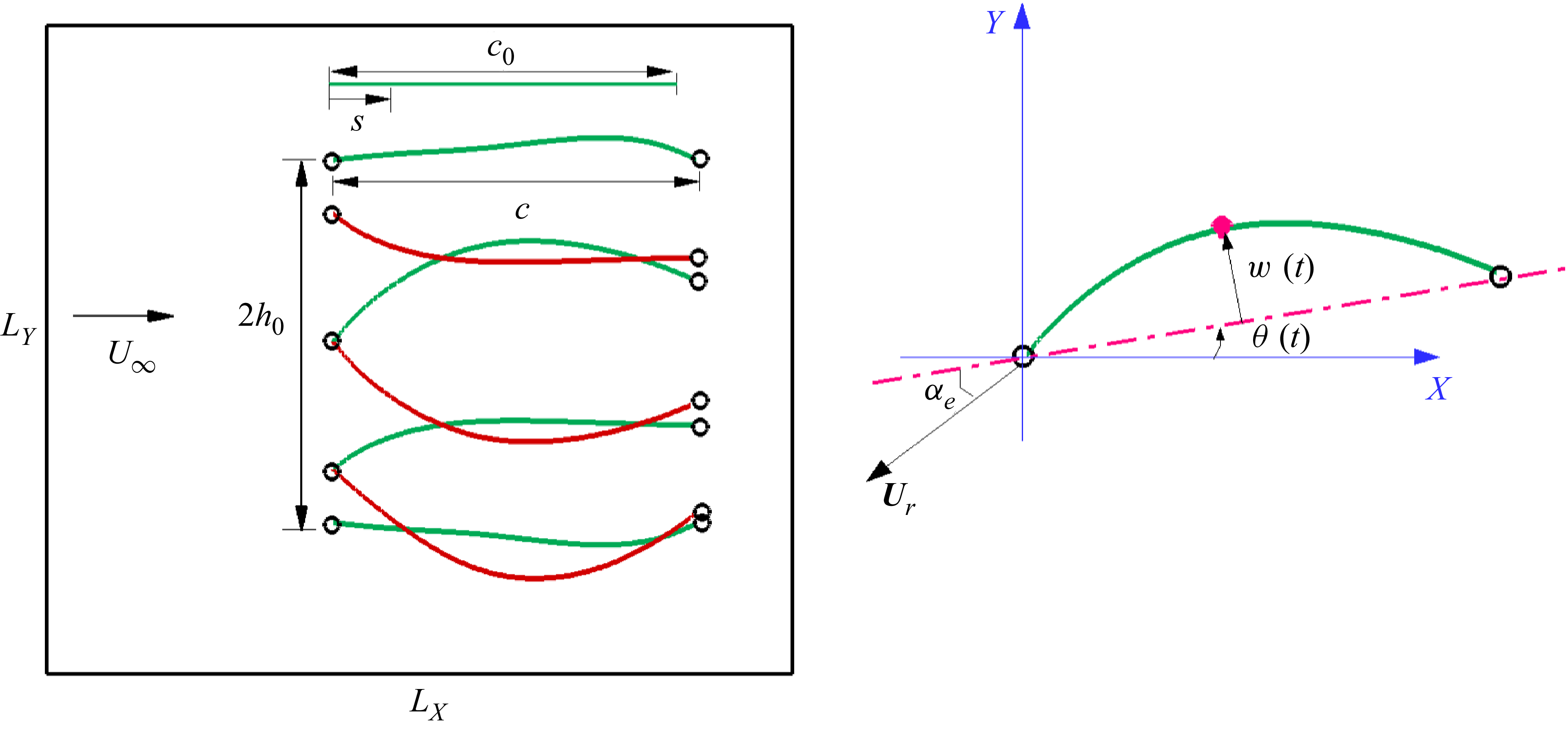


 Open access