

Many murine research studies report digestible energy (DE) and/or metabolisable energy (ME) intake from natural-ingredient diets. These should preferably be determined in an in vivo study from food intake, faecal output, and, for ME intake, urine output, and each component’s gross energy (GE) density(Reference Tobin, Schuhmacher, Hau and Schapiro1). These measurements require specialist equipment and cages and appropriate expertise(Reference Tschop, Speakman and Arch2–Reference Armitage, Hervey and Rolls6). Only a few laboratories that regularly perform energy metabolism studies meet these requirements. Consequently, investigators often estimate energy intake by one of two indirect methods.
First, they may multiply the food intake by the diet’s energy density estimated from Atwater factors applied to the composition of the diet(Reference Atwater7). The values are 4 kcal/g protein and carbohydrate (carbohydrate includes fibre) and 9 kcal/g fat; the equivalent SI values are about 16·7 and 37·7 kJ/g, respectively. Atwater obtained the values (also called physiological fuel values) from studies with humans fed typical diets. Subsequently, Merrill and Watt(Reference Merrill and Watt8) slightly modified the values for different foods. Despite the widespread use of Atwater factors, there are doubts about their accuracy, even for human foods(Reference Merrill and Watt8–Reference Maynard10). Furthermore, they assume a high nutrient digestibility, typical of refined human foods. Bielohuby and colleagues(Reference Bielohuby, Bodendorf and Brandstetter11) have confirmed that Atwater factors are inappropriate for lower digestible, natural-ingredient murine diets. Second, investigators may also use ME density estimates from diet manufacturers’ data sheets. However, with a few exceptions, these are based on Atwater factors and have the same disadvantages.
At about the same time as Atwater’s work on human foods, agriculturists were also developing a means of predicting the energy content of natural-ingredient animal feed and diets that allowed for differences in digestibility. Foremost in these methods was estimating ME density from total digestible nutrients, in which Atwater factors were fitted to the digestible nutrients(Reference Schneider12,Reference Crampton and Harris13) . However, since the 1960s, direct measurement of DE and ME has become the standard method of energy evaluation in the USA and most of Europe(Reference Flachowsky and Kirchgessner14).
This change in energy evaluation methodology and the widespread availability of computers in the 1960s led to the development of energy predictions from multiple regression analysis, with dietary nutrients as covariates. Initially, the covariates were digestible proximate or Weende nutrients, usually to comply with regulatory requirements(Reference Eeckhout and Moermans15). The Rostock group was at the forefront of developing such predictions in the 1960s. Their data have been summarised in a compendium by Schiemann(Reference Schiemann, Nehring and Hoffmann16) and two recent reviews(Reference Jentsch, Beyer and Chudy17,Reference Jentsch, Chudy and Beyer18) . Their work formed the basis of the currently recommended means of predicting the ME density of pig diets in Germany from digestible(19) and crude nutrients(20).
Routine measurement of digestible nutrients is impracticable and arguably more difficult than directly determining ME density. Consequently, chemical analysis of crude nutrients began to replace digestible nutrients in prediction equations(Reference Morgan, Cole and Lewis21). The crude nutrients ranged in complexity from those in the simple proximate or Weende analysis (crude protein (CP), ether extract (EE), crude fibre (CF), ash and nitrogen-free extractives (NFE)) to those based on more complex fibre types (neutral detergent fibre (NDF), acid detergent fibre (ADF), and soluble carbohydrates (starch, sugars)(Reference Eeckhout and Moermans15,Reference Just, Jørgensen and Fernández22–Reference Kirchgessner and Roth25) . While each laboratory provides one or more valid equations, they reflect the laboratory’s specific conditions, such as the age and weight of animals, the techniques used and environmental conditions. Applying predictions more widely from an individual laboratory underestimates the likely prediction errors(Reference Noblet and Perez24). Unfortunately, investigators often fail to consider the size of prediction errors when drawing conclusions from studies in which one or more variables, such as energy intake, are estimated rather than measured.
Our study aimed to improve ME density estimates of murine diets. We had hoped to base these estimates on data obtained in rats and mice, but this proved impractical. Consequently, the emphasis switched to the suitability of data from pig studies for murine prediction equations. Several studies suggested this might be practicable(Reference Furuya, Takahashi and Kameoka26–Reference Jørgensen and Lindberg28).
Our first step was to confirm the similarity of digestibility of nutrients in the pig, rats and mice that would justify using predictions of DE and ME density of natural-ingredient diets from pig studies for murine models. Second, if so, we intended to create prediction equations for energy density in pigs from many published studies using grower/finisher (GF) and adult (AD) pigs. The predictors were to be those commonly reported in four typical analytical packages for diets. The number of data records is greater than in previous studies. All the data are measured, not calculated, from various geographical areas and research groups. Two other recent publications have taken a similar approach by obtaining data from a wide range of sources(Reference Sung and Kim29,Reference Choi, Sung and Kim30) , though there were no equivalent prediction equations for dietary ME density. A critical function of our study was to estimate how well our equations fitted the existing data and their accuracy in predicting dietary ME density from future analytical data.
Materials and methods
The study comprised two phases, each requiring distinct sets of data. These phases are listed below, along with a description of the data used and statistical analyses applied to the data. Typically, we used R Statistical Software v 4.2.3(31) and its various packages. We installed the packages and loaded their library of procedures into RStudio (http://www.rstudio.com/). We provide the list of packages in the online Supplementary Material. We occasionally supplemented these methods with statistical software packages described in the text. Although R is open source software, we recognise that some readers prefer ‘plug and play’ software to using such code. We identify comparable software in the online Supplementary Material. Some of our methods are not readily available, and we have provided the code we used in those cases.
Phase 1. Evidence that energy digestibility in pigs and rats is similar
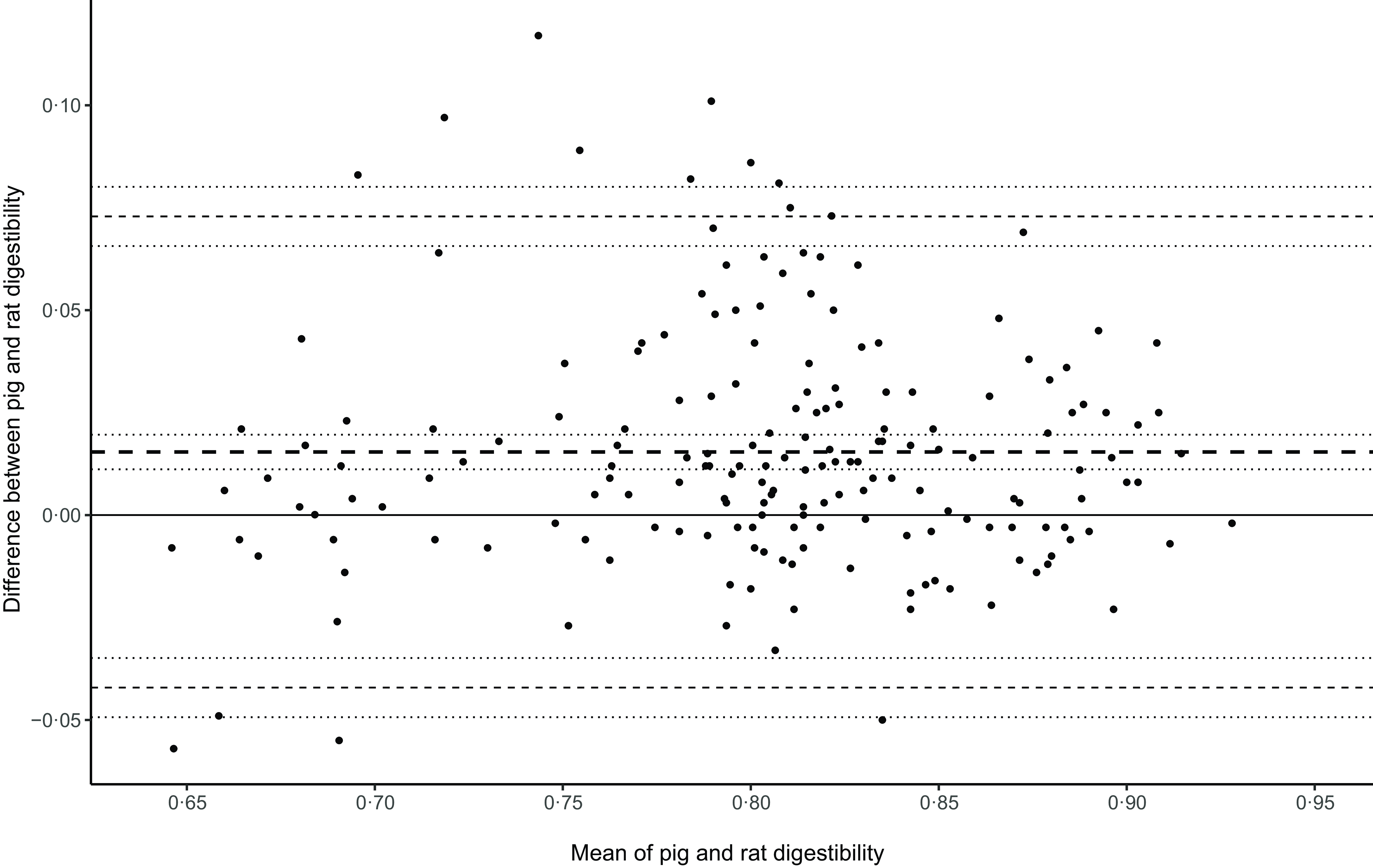
Energy digestibility is the major contributor to ME density. To justify using pigs as a model for murine ME density, we must first demonstrate good agreement between the DE or ME density of diets fed to murine and pig models. We obtained twelve papers containing measurements of energy digestibility in diets or ingredients fed to both pigs and rats. These papers contributed 204 data pairs (we excluded two pairs, based on feeding palm kernel products, as substantial outliers). The references are given in the online Supplementary Material. We used the Bland–Altman plot to assess the agreement in energy digestibility between pigs and rats(Reference Altman and Bland32–Reference Ludbrook34).
Phase 2. The development of predictive estimates of dietary metabolisable energy density based on dietary chemical analysis
Data sources and selection
We used PubMed, Google Scholar and apt journals to obtain papers that included measurements of ME density and relevant chemical analyses. The list of papers used is provided in the online Supplementary Material. For consistency, we refer to each entry containing the analytical observations in a diet or ingredient as a record and the collection of records as a database. We describe any subgroup of the database as a dataset. The first division of the database is into four datasets representing different chemical analysis groups. For simplicity, we refer to the groups in the text as the CF, NDF, neutral detergent fibre plus starch (NDFS) and neutral detergent fibre plus starch and sugars (NDFSS) datasets. Table 1 shows the nutrient components of the four groups. Each of the four groups includes a residue value, the difference between the total DM and the sum of the measured analytes. The residues were NFE, non-fibrous carbohydrates (NFC) and Residues 1 and 2. The number of papers used in each dataset was CF, 55; NDF, 80; NDFS, 31; and NDFSS, 8. Several papers contained all these carbohydrate measurements. The data were standardised to a 100 % DM basis and expressed as g/100 g for chemical analytes and kJ/g for energy density.
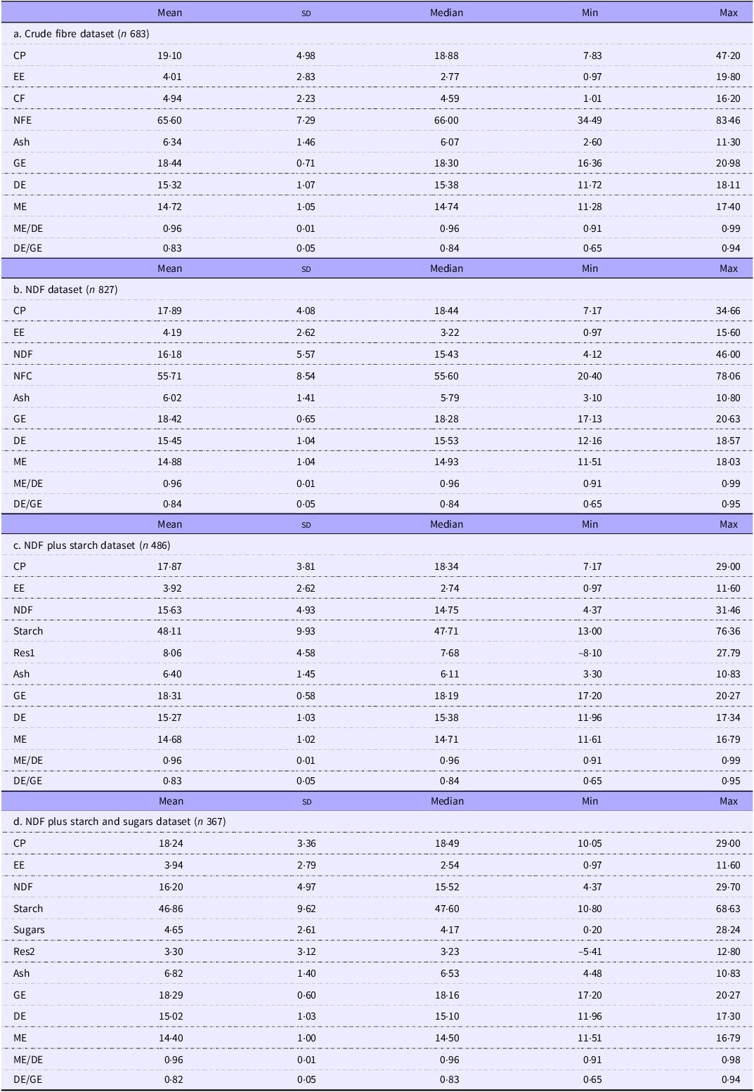
Descriptive statistics for four datasets from which outliers have been removed. The chemical analyses are expressed as g/100 g of DM and energy values as kJ/g of DM. The abbreviations for the nutrients and energy forms are defined in the abbreviations section
With a few exceptions, we excluded ingredients from our source data. Although several investigators have argued that chemical analysis and energy density measurements of ingredients can contribute to dietary energy density predictions (additivity)(Reference Morgan, Cole and Lewis21,Reference Morgan, Whittemore and Phillips23,Reference Morgan and Whittemore35–Reference Noblet, Fortune and Dupire39) , it is not a universal view. Additivity may be invalid in several circumstances. First, when ingredients have a nutritional profile very different from the mixed diet(Reference Noblet and Henry40) or when mutual supplementation of proteins or amino acids supplementation affects urinary energy excretion and metabolisability(Reference Kerr and Easter41,Reference Tobin and Carpenter42) . Finally, the methods used to determine the energy density of ingredients may commonly contain errors(Reference Noblet, Wu and Choct43–Reference Kong and Adeola45). We had sufficient records from diets to generally avoid the need to include ingredient data. The exceptions were those where the ingredient contributed to almost the entire diet, only supplemented with minerals and vitamins.
Murine diets
We found thirty-four records in six papers that reported measured dietary ME density and appropriate chemical analysis obtained with rats or mice, though for the CF model only. The number of records is too few to provide reliable regression equations: a minimum of 10–20 records is required per independent variable(Reference Harrell46) and possibly more(Reference Riley, Ensor and Snell47). Consequently, we limited our data to those from pig studies.
Pig diets
We only included data from pigs in the GF (25–125 kg) and AD phases (usually sows weighing over 200 kg). For most analyses, we combined the data from the two groups. Occasionally, authors duplicated records in more than one paper, and we excluded them to prevent any bias or data weighting. We also eliminated outliers using the methods described in statistics. Regrettably, we excluded many potentially valuable papers because they lacked some analytical component(s), often EE or ash. Sometimes, we could retain such papers with additional information from the authors.
Statistical analyses
Data description
We used the R data summary function to obtain descriptive statistics of the four analytical datasets for the combined GF and AD phases. These descriptives are shown in Table 1.
ANOVA
Where an ANOVA was necessary, we first tested for normality using a Q-Q plot and the Shapiro–Wilk test. The appropriate ANOVA test depended on the outcome, with the Welch ANOVA test preferred for parametric data and the Kruskal–Wallis test for non-parametric data.
Removal of outliers with the isolation forest method and extreme standardised residuals
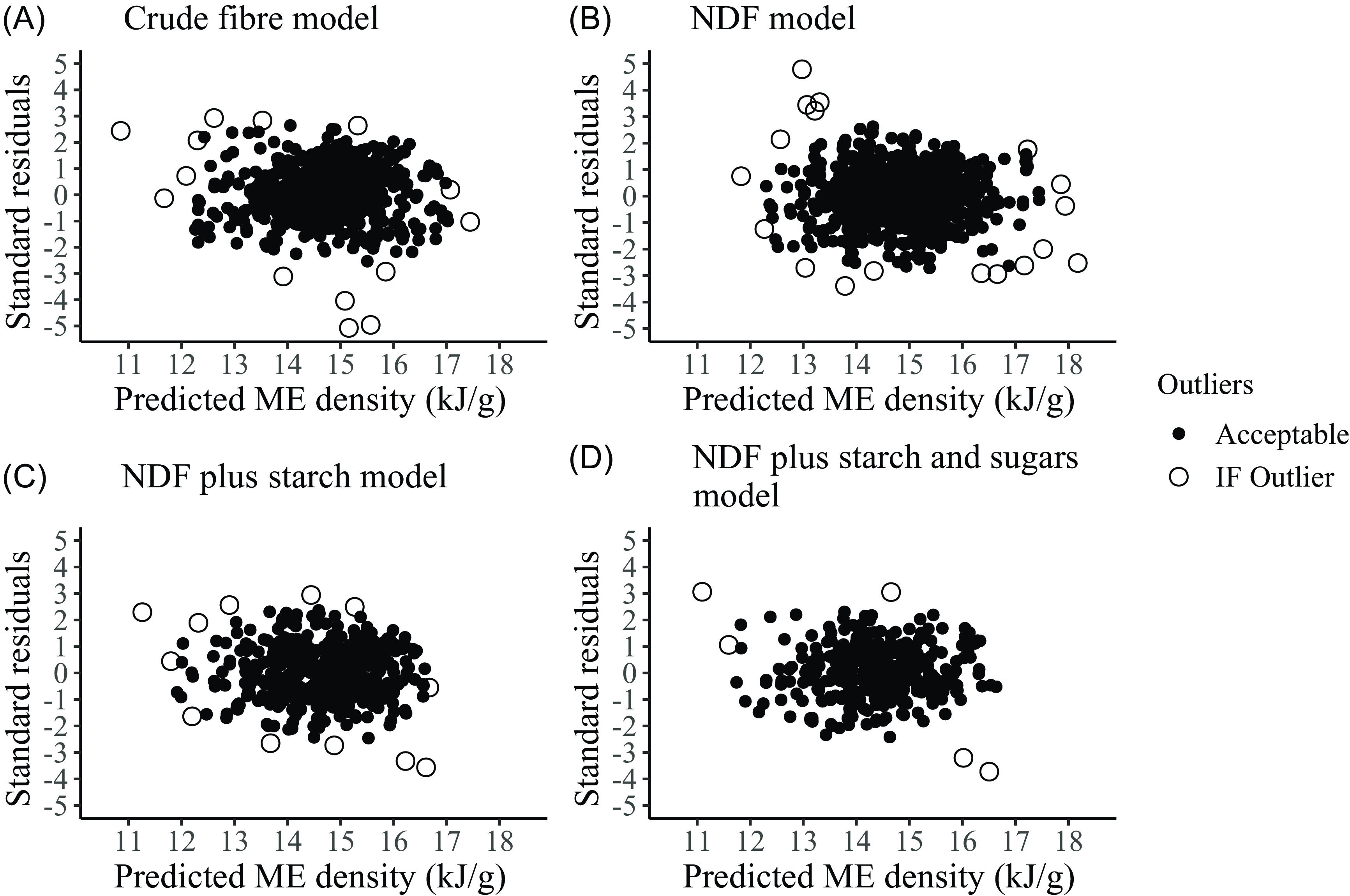
We excluded outliers from the four datasets using the isolation forest method(Reference Liu, Ting and Zhou48) as described here. We initially used multiple regressions to analyse the records in each dataset (CF, NDF, NDFS and NDFSS). The dependent variable was ME density, with the chemical analyses as the covariates. The analysis created a predicted ME density and its standardised residual (the distance of the actual value from the prediction divided by the standard deviation of the residuals) for each observation. We then applied the isolation forest procedure to the pairs of predicted ME density and standardised residuals using the solitude package in R. The isolation forest process can be envisaged as randomly drawing horizontal and vertical lines through a scatter plot. The number of lines required to isolate each point from adjacent ones is recorded. The exercise is repeated, in our case, 100 times, but ‘starting’ the line in a different location each time. Only a few lines are necessary to separate outliers, while those in a cluster need many more (see the illustration in Liu et al. (Reference Liu, Ting and Zhou48)). The process then allocates an anomaly score to each point based on the average number of ‘cuts’ or divisions required to isolate it. The score is standardised and ranges from zero (not anomalous) to one (anomalous). The dividing score between points being definitely anomalous or not anomalous is 0·5. We considered records with an anomaly score of about 0·65 and above as outliers. We used a rigid procedure to ensure an unbiased exclusion of outliers across all datasets.
Multiple regression analysis
We used several R packages and functions to obtain the statistics for the multiple regressions and goodness-of-fit (GOF) measurements. We have included a list and their purpose in the online Supplementary Material.
Collinearity and variable selection
Collinearity occurs when a regression has a high correlation between two or more predictors(Reference Belsley, Kuh and Welsch49). It is generally assumed to increase the CI and P value and decrease the precision of regression coefficients. Compositional data such as ours (where the predictors add up to 1 or 100) present a severe problem with collinearity, and regression analysis using all the predictors becomes impracticable. We applied the standard solution of removing a predictor – the ‘drop-one’ approach. This process, including the choice of predictor, is discussed further in the correlation matrices section of the results.
We assessed the risk of collinearity in two ways. First, we used a correlation matrix to examine the degree of correlation between pairs of predictors. Although we describe the pair-wise correlations in the results, the tables are in the online Supplementary Material. If there is significant collinearity, the highest correlated pair usually becomes the candidate from which one predictor is dropped. Second, we determined each coefficient’s variance inflation factor (VIF), which is a more effective method. The VIF reports the overall association between predictors rather than between pairs, as shown in the correlation matrix. One would typically consider dropping the predictor with the highest VIF to avoid collinearity. We tested for detrimental effects of collinearity on coefficients using a measure of s e adjusted for their size. We term this the CV of the se (CVse), calculated as 100 × se/mean. The values are shown in the online Supplementary Material.
Assessment of potential laboratory bias
To test for potential bias in our regressions from data from one or more laboratories, we allocated each record to one of eight Lab groups that might use similar pigs and have a common approach to environmental conditions and techniques (e.g. Noblet’s group). Lab group 0 was the reference group made up of a large number of records from unconnected research groups. We measured potential laboratory bias from the variation in specific laboratory estimated marginal means (EMM) and contrasts after multiple regression analysis with Laboratory as a factor. The EMM is the mean ME density when one applies the regression equation to the subset of predictors for a particular laboratory. The factor also gives the difference (contrast) between the EMM value for each laboratory and the reference Lab 0 (see online Supplementary Material). We statistically compared the EMM and contrasts before and after outlier removal across the four datasets.
Regression analysis methods using intercept and no-intercept models
After checking for bias and outlier removal, we performed intercept and no-intercept (regression through the origin) multiple linear regressions for the four analytical datasets for both GE and ME density. Regression models are rarely used to predict GE density. However, the model is a valuable check on the data and regression model since one can match the predicted coefficients against well-established estimates of the energy content of the primary nutrients.
Intercept model: We analysed the combined GF and AD data incorporating Phase (GF, AD) as a factor. The regression analysis gives identical nutrient coefficients for both GF and AD animals. The coefficient for the Phase represents the additional energy AD animals obtain from a diet compared to the GF animals. The additional energy should only be added to ME density predictions for AD animals.
No-intercept model: Many statisticians advise against the no-intercept model since it weakens the regression fit to the data(Reference Eisenhauer50). However, we use it here to estimate the relative contribution of energy-containing variables to the overall energy density(Reference Tay-Zar, Wongphatcharachai and Srichana51,Reference Noblet, Van Milgen and Chiba52) , and thus, ash is excluded as an independent variable. Unfortunately, the no-intercept model cannot account for external variables, such as the growth phase, effectively substituting these variables with a pseudo-intercept value. Consequently, when we used a no-intercept model for ME density, the GF and AD animal data were analysed separately. That was not necessary for GE density since this is unaffected by Phase.
Goodness-of-fit estimates
We determined various measures of GOF of the regressions. We used the adjusted coefficient of determinations (R 2, the Ezekiel estimator(Reference Leach and Henson53)) to express the proportion of variation in the dependent variable accounted for by the independent variables. Unlike the coefficient of determination (R 2) derived from the Pearson correlation coefficient (r), it compensates for what otherwise would be an increase in value caused simply by adding additional independent variables. Adjusted R 2 thus allows us to compare the GOF in models with different numbers of independent variables. We also included predicted R 2 (see the section on validation). However, we excluded R values for the no-intercept models since they are inflated by the standard calculation method and provide an unreliable estimate of their relative performance(Reference Kozak and Kozak54).
We also determined the root mean square error (RMSE) and residual standard deviation/error (RSD/RSE/sigma are used interchangeably). Although RMSE and RSD are closely related, they have slightly different uses. Outliers affect RMSE more than RSD, and a few extreme values may introduce considerable bias. Since we removed extreme outliers, RSD is more appropriate here, though we retain RMSE for comparison with other studies.
The two groups of values provide a convenient juxtaposition: R 2, with a scale of 0 to 1, estimates the variation explained by the independent variables. In contrast, RMSE/RSD represents the unexplained variation, with units in which the dependent variable is reported.
We also included MAE (the mean absolute error), a simple but useful measure. It is the average mean absolute difference between the predicted and actual values from the regression. Its derivative mean absolute percentage error is the mean absolute difference expressed as a percentage of the actual value. Finally, we analysed the Akaike information criteria to identify a model that most accurately fits the data without overfitting (i.e. it avoids identifying a regression that fits the existing data very well but at the expense of providing an optimum prediction of new data). It actively penalises any superfluous additional independent variables. The smaller the value, the better the model. Thus, an increase in the R value(s) and a decrease in RMSE, RSE/RSD, MAE, mean absolute percentage error or Akaike information criteria indicate an improvement in the fit of a regression model.
Assessment of the regression models in estimating metabolisable energy density
The variation in the number of laboratories contributing to the data in each of the four analytical regression models restricted our ability to determine the models’ relative accuracy. However, our data included 359 records that contained the full range of analytes. We calculated the predicted ME density for each of the records of the four regression analytical models. The GOF measurements, particularly the MAE, gave unbiased estimates of the accuracy and precision of the four models. We used two further statistical tests to determine the differences in absolute residual values. The two tests were an ANOVA, as described above, and a test of equivalence using a multiple-sample TOST test provided in the InVivoStat software package (https://invivostat.co.uk/). Equivalence testing increases the confidence that two or more treatments (their means and 95 % CI) are equivalent within stated bounds, in our case about 2 %, rather than simply not significantly different as in an ANOVA(Reference Anderson-Cook and Borror55).
Validation: the accuracy and precision of the regression analyses for future sets of data
Although it is common to describe regression equations as predictive, they only explain the data on which they are based and may be of doubtful accuracy for a predictive model. Investigators often overlook the subtle difference between the explanatory and predictive functions(Reference Yarkoni and Westfall56). The change in function does not affect the regression coefficients themselves. The main effect is on GOF and the magnitude of explained and unexplained variation: this can be a severe problem with small datasets. We tested the predictive quality of our regression in two ways.
The most comprehensive method was the k-fold cross-validation(Reference Stone57,Reference Geisser58) with a k value of 10: the analysis is provided in the R caret package. The procedure assumes that one can mimic a future set of data that complies with the characteristics of the current population. The existing data are divided into k portions or folds. The estimated ME density of records from each of the ten portions (‘the future dataset’) is obtained from predictive equations from the remaining nine data portions. This procedure produces ten estimates of one or more measurements of the GOF. As a default, caret provides R 2, RMSE and MAE as GOF indices. We extended the code to add adjusted R 2 and RSD (the code is shown in the online Supplementary Material). We repeated the procedure ten times to improve the reliability of the values. Our mean values and their 95 % CI were thus obtained from 100 estimates. We also obtained the predicted R 2 using the olsrr R package. This value is a simpler validation measure based on dividing the dataset into a training and evaluation group. After that, the procedure is similar to the k-fold cross-validation, but it only provides a single estimate of R 2.
Results
Phase 1. Evidence that energy digestibility in pigs and rats is similar
The preliminary data assessment shown in the online Supplementary Material showed good agreement in the energy digestibility of pigs and rats above 0·65D. Nineteen pairs of data below 0·65D were considered outliers and excluded. Figure 1 displays a Bland–Altman plot of the remaining 185 pairs of combined datasets above 0·65D. Although the bias differed significantly from zero with a 95 % CI of 0·01–0.02, the biological difference was negligible, with digestibility in pigs about 0·015 units greater than in rats. This bias amounts to about 2 % of our data’s typical digestibility of 0·83. The outer levels of agreement were –0·042 to 0·073. Our interim conclusion was that we could proceed and use pigs as a model for murine models if digestibility was greater or equal to 0·65.
The relationship between published energy digestibility measurements in rats and pigs illustrated as a Bland–Altman plot. The inner dashed line is the bias, and the outer dashed lines are the upper and lower limits of agreement. The dotted lines around each line are the 95% CI

Phase 2. The development of predictive estimates of dietary metabolisable energy density based on dietary chemical analysis
Removal of unsuitable and anomalous data
We excluded eight records before statistical analysis. Five records had a DE:GE ratio of less than 0·65 and were outside the range of agreement between pig and murine digestibility; one of the five had an unusual ME/DE value of less than 0·90. We deleted three records from a single laboratory from the NDF and NDFS groups because of doubts about the accuracy of the analytical data (the sum of the measured analytes substantially exceeded the DM).
Removal of outliers
The number of statistical outliers identified and excluded in the four datasets using the isolation forest method was less than 2·5 %: CF, 14 of 697 (2 %); NDF, 18 of 845 (2·1 %); NDFS, 12 of 498 (2·4 %); and NDFSS, 5 of 372 records (1·3 %) (Fig. 2).
Identification of outliers in the ME density data for the four regression models using the isolation forest technique. ME, metabolisable energy; NDF, neutral detergent fibre.
Dataset descriptive statistics
Table 1 shows the descriptive statistics for the four groups after outlier removal. The nutritional values encompass those of typical murine breeding, general-purpose and maintenance diets. Removing outliers had a small effect on the analyte concentrations, with a mean difference of –0·40 % (sd 0·78) of the values in the equivalent original dataset. We were concerned to see negative minimum values for Res1 and Res2 in a few records, some of which occurred in laboratories we considered to be highly competent. Negative residue values indicate an error in one or more measured analytical variables. However, we retained these records to avoid unintended bias since these analytical discrepancies might be present in other records but less visible.
Correlation matrices
We have provided the full matrices in the online Supplementary Material. The correlation matrices are an objective method for deciding which pair of predictors to use in the ‘drop-one’ approach in regressing compositional data. While the correlations between ash and residues for the CF (–0·65) and NDF (–0·58) models support dropping ash or the residue, that is less so for the NDFS (0·17) and NDFSS models (0·41). In the latter two models, substituting ash and starch is statistically the best option but unhelpful when starch is an important predictor to study. We consider context to be an important consideration in our choice. Thus, for compatibility with previous studies and consistency across our models, we removed either ash or the calculated residue (NFE, NFC, Res1 or Res2) from all four dataset regressions. We refer to the options as ash-based and residue-based models. We describe our approach to choosing between the two models in the regression collinearity section below.
The matrices also provided other nutritionally interesting associations. There was a high correlation (0·98) between DE and ME density measurements across the four analytical datasets. Some authors included ME values calculated from DE, which inevitably influences the correlation. Nevertheless, there is undoubtedly a close relationship. The correlations between GE and DE or ME density were poor (0·29–0·47). The EE was consistently highly correlated with GE (0·79–0·92) but not DE or ME density. Both DE and ME were moderately negatively correlated with ash (–0·40 to −0·62), probably because ash is the inverse of energy-containing organic matter. Energy digestibility (DE/GE) consistently showed a high negative correlation with CF or NDF (–0·67 to −0·77) and a moderately positive one with NFC or starch (0·59–0·64). The typically low levels of sugars had no effect.
Of the nutrient-nutrient correlations, only two exceed the cut-off of 0·8–0·9 associated with a possible collinearity problem(Reference Mason and Perreault59). These were CP and NFE (–0·80) in the CF dataset and starch and ash (–0·81) in the NDFSS dataset. The remaining correlations ranged from −0·73 to 0·54, with a mean absolute value of 0·31 (sd 0·21).
Regression analyses
Unless otherwise stated, the comments refer to the regression models after removing outliers.
Regression collinearity and variance inflation factors
In addition to the correlation matrices, we assessed the risk of collinearity of the regression coefficients using VIF. VIF values, and thus collinearity, were much lower in the ash-based than residue-based models (Table 2a–d). The effect of VIF on the precision of a calculated coefficient was estimated from the CVse as described in the Materials and Methods. Despite the higher VIF values in the residue models, there was no statistical difference between the precision of the coefficients in the ash- or residue-based regressions across the four models (t test with unequal variances, t = 2·06, P = 0·26, df = 25). The complete data are shown in the online Supplementary Material.
Gross and metabolisable energy regressions after removal of outliers, with the grower/finisher animals as the reference phase. The values in brackets are the 95 % CI. Unless otherwise stated P < 0·001. When the coefficients are applied to nutrients expressed as g/100 g diet DM, the unit of energy density will be kJ/g DM. Phase AD: the additional energy to be applied to the predicted energy digestibility when used for older animals. The variance inflation factor (VIF) values are identical for the gross and metabolisable energy density regressions
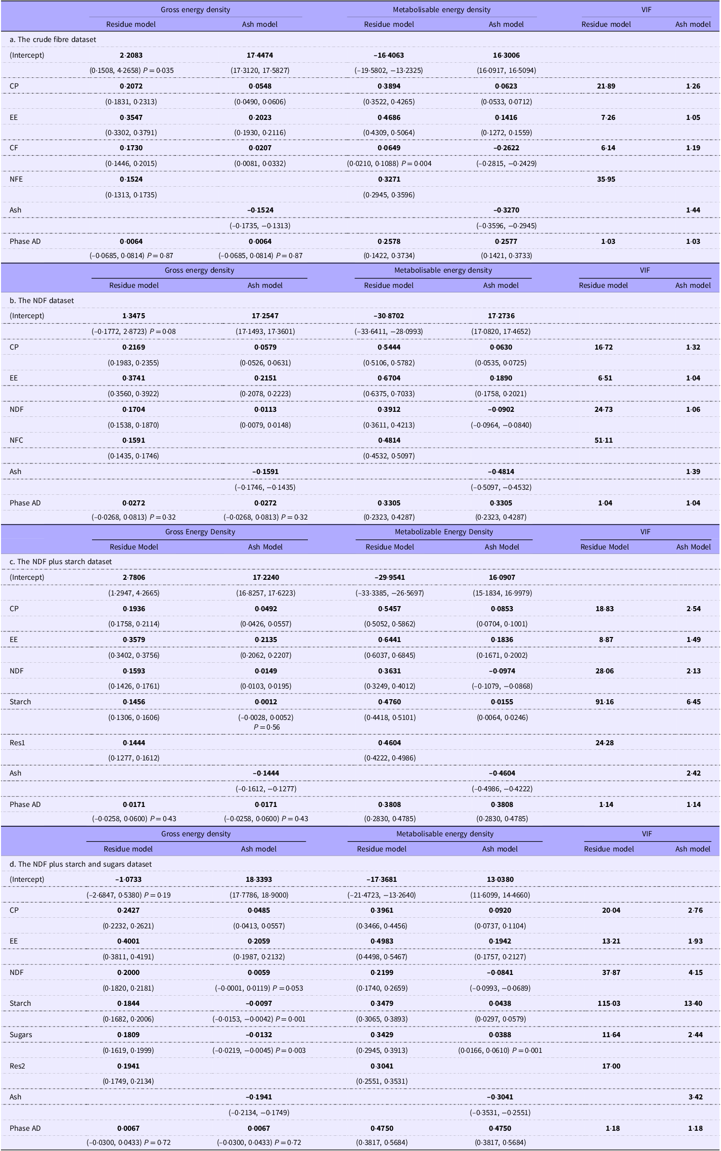
Note: We highlighted the coefficients to distinguish them from the other numbers. The coefficients are those numbers most likely to be extracted from a reader to create prediction equations.
Although using the ash models avoids the issue of collinearity, it can produce coefficients that, while mathematically correct, appear biologically odd. For example, in the NDFS GE density model, starch has a coefficient of zero with P = 0·54. Although the VIF in the residue-based models is high, the effect is moderated by the high R 2 values and the large sample number, as described in the Discussion. The adjusted R 2 for ME density regressions for the four models varies from 0·751 to 0·869, with 367–827 records. Thus, in this study, VIF values exaggerate the risk of detrimental collinearity. However, since using the residue model is not universally accepted, we have included both ash- and residue-based intercept regressions below. The predicted energy densities and GOF values are the same in both cases.
Regression models
In summary, we created intercept and non-intercept regressions for dietary GE and ME density from four datasets (CF, NDF, NDFS and NDFSS). Table 2a–d shows the nutrients included in each. Each intercept regression included the ash- and residue-based alternatives.
The effect of potential laboratory bias
After removing outliers, the mean difference in estimated marginal means (EMM) between the laboratory groups and Lab group 0 across the four datasets was 0·02 kJ/g (sd 0·28 kJ/g), which represents approximately 0·1 % of the average dietary ME density (online Supplementary Material). We concluded we could ignore any Laboratory group bias and analyse the data as a whole.
Regression parameters
Intercept models
Table 2a–d shows regression analyses on the four datasets from which outliers have been excluded. Removing outliers had a negligible effect on the coefficients (typically 1–3 % at most). The coefficients for the individual intercept models shown in the tables require little comment. The intercept for most GE density models based on residues was not significantly different from zero. The exception was that for the NDFS regression: nevertheless, it was small (c 2.8 kJ/g, CI 1.3, 4.3). The intercepts for the ash models were substantial (generally 17–18 kJ/g) and significant (P < 0·001).
The predictor coefficients for GE and ME density were highly significant (mainly P < 0·001) with two exceptions: (a) starch in the GE and ME density NDFS ash models (P = 0·56) and (b) NDF in the GE density NDFSS ash model (P = 0·053). Although many ME density regressions have negative coefficients for CF, we observed it only in the ash-based model (and the no-intercept model below). However, even when not negative, the ME coefficients for CF were much lower than the biological estimate of 7·54 kJ/g (Table 3).
Calculated gross energy (GE) and metabolisable energy (ME) density of nutrients
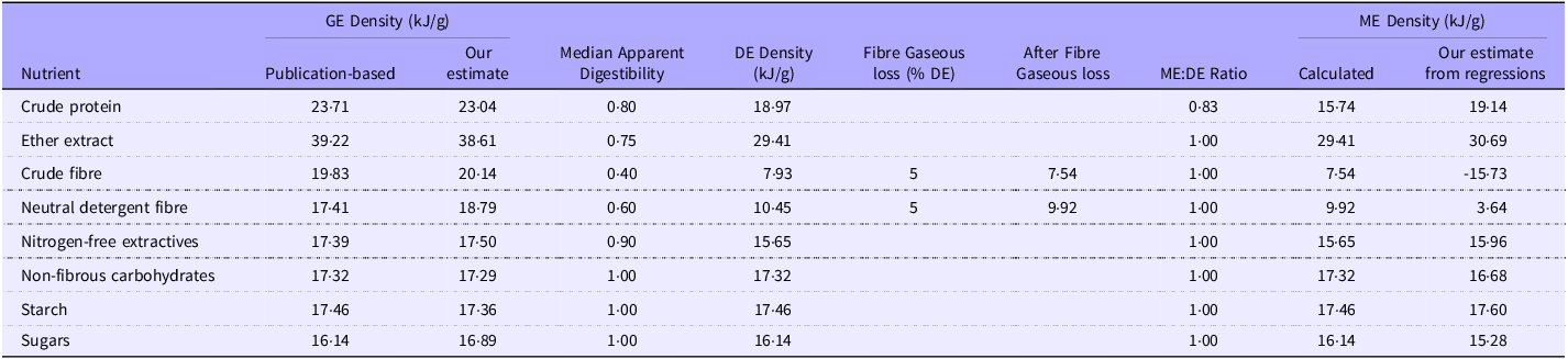
1Our estimates of GE and ME density are taken from the non-intercept models, using mean values where possible. The ME values were from the grower/finisher data only.
2The basis for the data taken directly or calculated from publications is provided in the supplementary data.
3The values are estimated for typical diets with a digestibility greater than about 0·7; the energy density values for protein and fat are likely to be substantially lower in high-fibre diets.
4We have rounded our estimates on nutrient digestibility to the nearest 0·05 to avoid suggesting that the values are more than informed estimates from the literature. They could vary by 0·05 to 0·1 units.
The age-related Phase AD coefficients for the GE density models were also consistently non-significant, close to zero and unaffected by the model. In contrast, those for ME density models were highly significant and much larger. The average age-related coefficient shows that older animals (as defined in the Materials and Methods) absorb an additional 0·37 kJ/g from a diet than the younger GF animals. The amount increased from about 0·25 to 0·48 kJ/g across the four models.
The coefficients for ash and alternative residues (and their t values, though not shown here) appear as mirror images across comparable regression models, a phenomenon not commonly reported in the literature. This pattern occurs when any one of a pair of predictors is substituted and is unrelated to their coefficient in the correlation matrix. Its cause is beyond the scope of this paper.
The individual nutrient GE density values determined with the residue models were about 95 % (sd 8 %) of their respective theoretical values (Table 3). We ascribe the slight discrepancy to the contribution of energy density from the intercept. In the case of the residue-based ME density regressions, the very high intercept values made any attempt to relate the coefficients with theoretical values pointless. There was no similarity between the coefficients and theoretical nutrient GE or ME density in the ash-based regressions. The most reliable comparisons of regression and theoretical values are with the no-intercept models reported below.
The goodness of fit of the intercept models
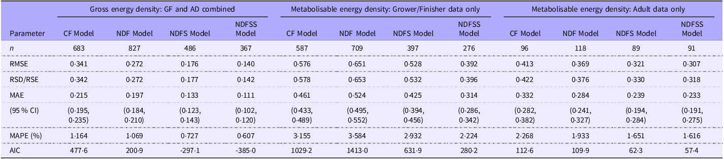
The GOF values for the intercept models are the same for the residue-based and ash-based models and are shown in Table 4a (GE density regressions) and Table 4b (ME density regressions).
Goodness-of-fit estimates for the gross and metabolisable energy density intercept-based regressions of the combined grower/finisher and adult data
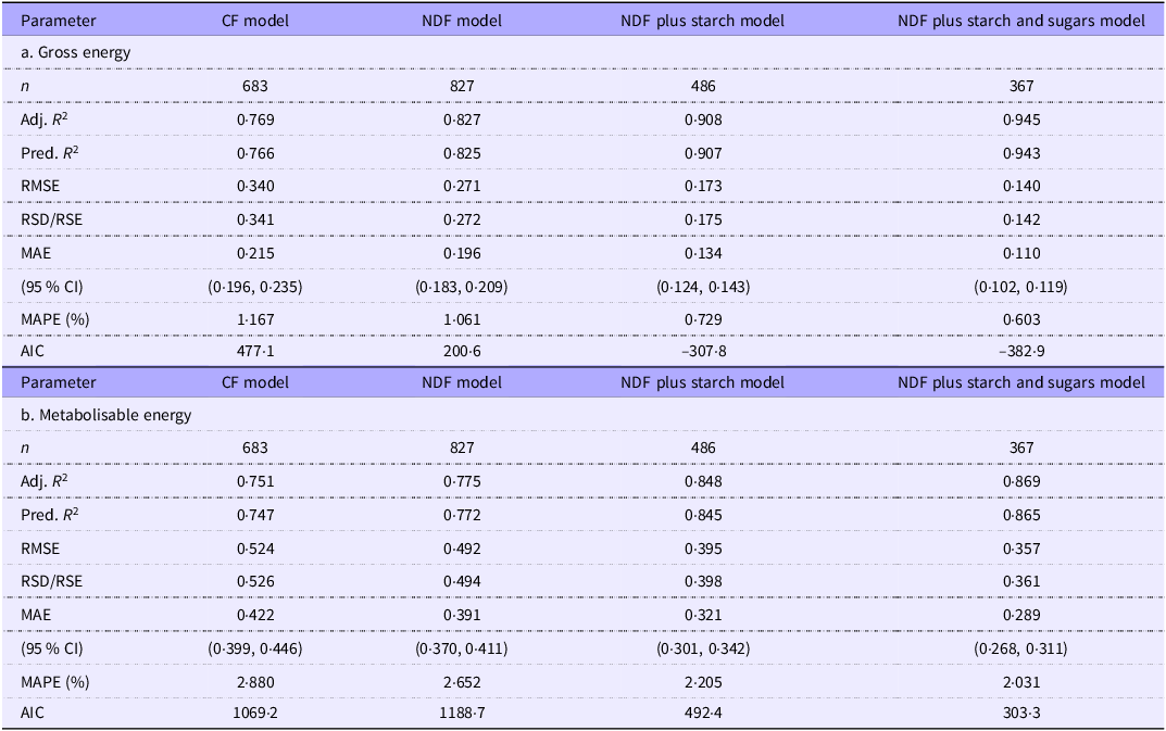
Removing outliers had little effect on the GOF values for the GE density regressions. The GOF progressively improved with model complexity. The predictors explain about 77–94 % of the variation in GE density, and unexplained variation is low. For example, RSD averaged 0·23 kJ/g, progressively decreasing with more independent variables in the models. The unexplained variation in the models represents only 1–2 % of the typical GE density of murine and pig diets (about 18·4 kJ/g).
Although we removed only about 2 % of the records as outliers, there was a modest improvement in the GOF of ME density regressions. The various R 2 estimates improved by about 2 % across the four groups, while RMSE and RSD values improved by 7 % and MAE and mean absolute percentage error by about 5 %. Not surprisingly, considering the additional complexity of measurement and variation in the metabolisability of the fibre components, GOF values were poorer in the ME density prediction models. Nevertheless, the independent variables still account for about 75–87 % of the variation in the dependent variable, which is good for most science-based studies(Reference Gupta, Stead and Ganti60). We comment in the Discussion section on the source of the remaining variation. The RSD values for the ME density regressions were 50–80 % higher than for GE regressions in the CF and NDF models and over 2-fold higher in the NDFS and NDFSS models. However, the MAE levels were low even in the more challenging ME prediction models and were only about 2–3 % of the ME density of typical pig or murine diets (14·8 kJ/g). The MAE was highest with the CF model, about 0·42 kJ/g (CI 0·40, 0·45), and this improved in the NDFSS model to about 0·29 kJ/g (CI 0·27, 0·31).
The GOF measurements across the four analytical models show that the CF-based model is the weakest fit while the NDFSS model is the strongest. This trend is not just a function of an increasing number of independent variables since the Akaike information criterion, which penalises such increases, substantially improves across the models. The NDFS model generated the largest single-step improvement in fit. Unfortunately, one must treat this comparison with caution since the number of laboratory groups (and hence potential variability) differs in the four models: we address this later when we analyse the GOF indices in 359 records that include all the analytes.
No-intercept models
The no-intercept models represent the net contribution of energy-containing nutrients to the regression. The merit of the no-intercept approach is that it generates biologically relevant coefficients, though they are still empirically based. However, the no-intercept model does not allow a meaningful coefficient for a factor like Phase: the outcome is a value tantamount to an intercept. Because of the expected insignificant effect of Phase on GE density in the intercept models, we have reported GE density coefficients in the no-intercept models on the whole data (Table 5a). In contrast, there was a significant Phase effect in the intercept-based ME density regressions, so we performed no-intercept ME density regressions for GF and AD animals separately (Table 5b).
No-intercept regressions. The data for the grower/finisher and adult animals are combined to estimate the gross energy density coefficients but reported separately for the metabolisable energy density coefficients (see text for explanation)
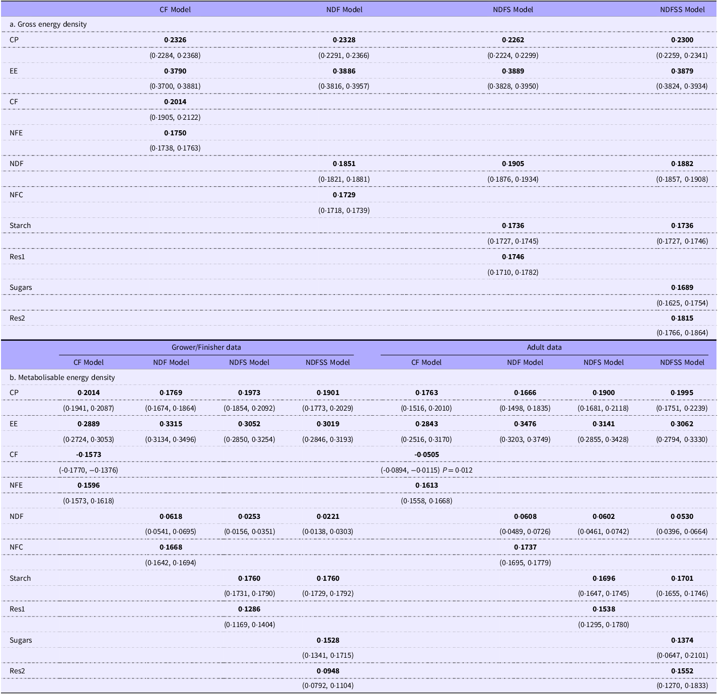
1Values in parentheses are the 95 % CI.
2Unless otherwise shown, the P values are < 0·001.
The percentage differences in the comparable coefficients after removing outliers were negligible (typically 1 %). The main exception was the CF coefficient in the ME density regression: this was probably a consequence of the small coefficient values and the relatively large effect of a small difference after outlier removal.
The GE density regression coefficients were similar to those of Noblet and Van Milgen(Reference Noblet, Van Milgen and Chiba52), and our theoretical estimates for CP, EE and carbohydrates were gathered from various publications (Table 3). The overall agreement with theoretical estimates was 100.6 % (sd 2.5 %). We could not find direct estimates of the ME density of individual nutrients, presumably because suitable experiments would be complex. However, we have calculated estimates of nutrient ME density from published data (Table 3). There were three points of interest: first, the regression values for the ‘available’ carbohydrates (NFE, NFC, starch and sugars) and EE were extremely close to the calculated values (mean 0·98, sd 0·03). Second, the regression values were much lower than theoretical for the fibre constituents (CF, NDF). Finally, the CP value was c.20 % higher from the regressions than theoretic values. Overall, the values were consistent with CF primarily affecting protein absorption with energy losses integrated into the fibre coefficients.
The goodness of fit of the no-intercept models
Outlier removal had little effect on the GOF values for GE density predictions (median improvement < 1 %) but improved those for ME density (median c. 5–6 %). Table 6 shows the GOF indices of the no-intercept models, which follow the same trend as the intercept models. The GOF values of the GE and ME density regressions generally improve with increasing model complexity. The difference between the CF and NDF ME density prediction models for GF pigs is an exception. However, the Akaike information criterion values show that the overall improvement is not just an effect of increasing the number of predictors. The GOF of no-intercept models for ME density is poorer than the comparable intercept models. The effect is most evident in the estimates of MAE, especially for the NDF and NDFS regressions. Despite the attractiveness of biologically relevant regression coefficients, the MAE values indicate that the prediction of ME density is slightly less accurate than the intercept model.
Goodness-of-fit estimates for the gross and metabolisable energy density no-intercept regressions of the grower/finisher and adult data in Table 5

1Values for R 2 are inappropriate for no-intercept regressions and are excluded.
Assessment of the regression models in estimating metabolisable energy density
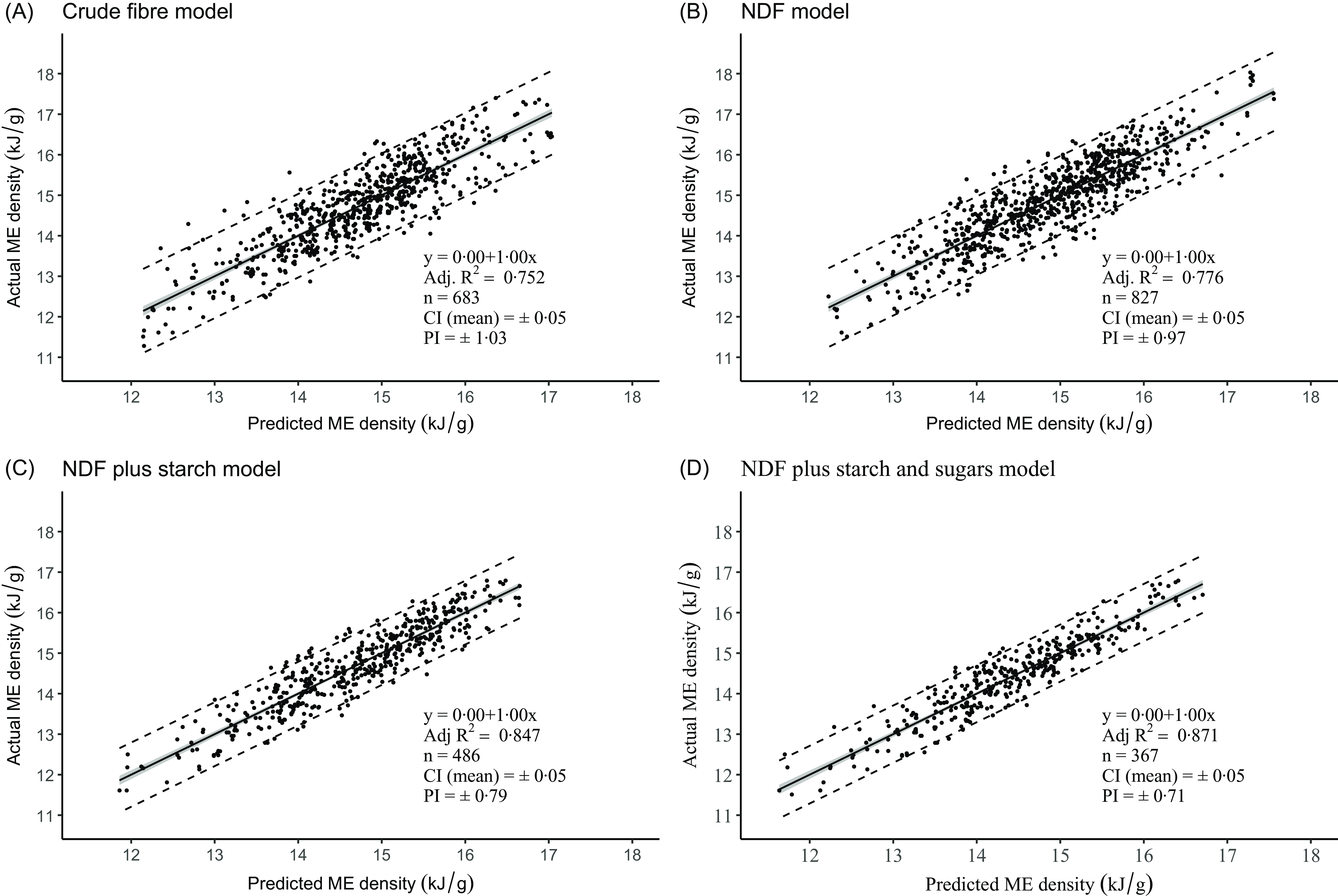
Figure 3 shows the regression plots of measured ME density on predicted ME density for the four models. We regressed the data in this order since it is important to understand how well the calculated energy density value represents the measured value. It is also the orientation recommended by Piñeiro et al. (Reference Piñeiro, Perelman and Guerschman61). In all four cases, the slopes were 1·00 and the intercept zero: these values demonstrate a perfect agreement between the mean predicted and actual values across the range of values studied. The 95 % CI of the prediction of the mean response (CI) in these regressions is small and not clearly evident in the figures. Although the CI is tapered, we have calculated its mean value as ± 0·05 kJ/g across all four regressions. Perhaps the best overall practical measure of the predictive accuracy of our regressions is the 95 % CI of the prediction of a single value (prediction interval, PI). It provides the range within which the true value of a prediction is likely to fall 95 % of the time. The PI are almost linear over the range of ME density values, so we can reasonably express them as a single value for each of the four analytical models. The PI were ± 1·03 kJ/g (CF), ± 0·97 kJ/g (NDF), ± 0·79 kJ/g (NDFS) and ± 0·71 kJ/g (NDFSS). These values represent a deviation from the average predicted ME value for the four models (14·8 kJ/g) of ± 7·0, 6·6, 5·3 and 4·8 %, respectively. As expected, the absolute PI are about twice the RMSE/RSD values.
Relationship between the measured and predicted ME densities in the four regression models. The inner shaded ribbon is the 95% CI, and the outer dashed lines are the 95 % prediction intervals. ME, metabolisable energy; NDF, neutral detergent fibre.
Choosing an optimum cost-effective regression model to estimate the metabolisable energy density
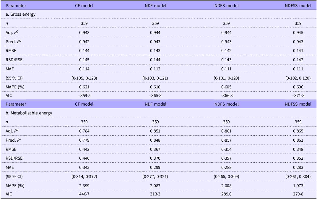
We obtained an unbiased estimate of the relative accuracy and precision of the four analytical regression models by analysing the 359 records present in all four datasets. Table 7 shows the GOF indices used. Notably, these regressions and GOF measurements come from a narrow range of laboratories with less diversity of factors such as animal breed, technique and measurement accuracy than records in the whole dataset. Consequently, it is unsurprising that the coefficients and GOF measures within these datasets are generally more precise than the equivalent whole dataset. The major exception is the regression analysis for the NDFSS dataset, in which the coefficients and GOF measurements in the two were very similar. However, the 359-records dataset included a substantial proportion of the NDFSS dataset. As with the primary data (Table 4), the GOF estimates improved with the complexity of the model.
Comparison of goodness-of-fit measures of the four datasets of common grower/finisher and adult records

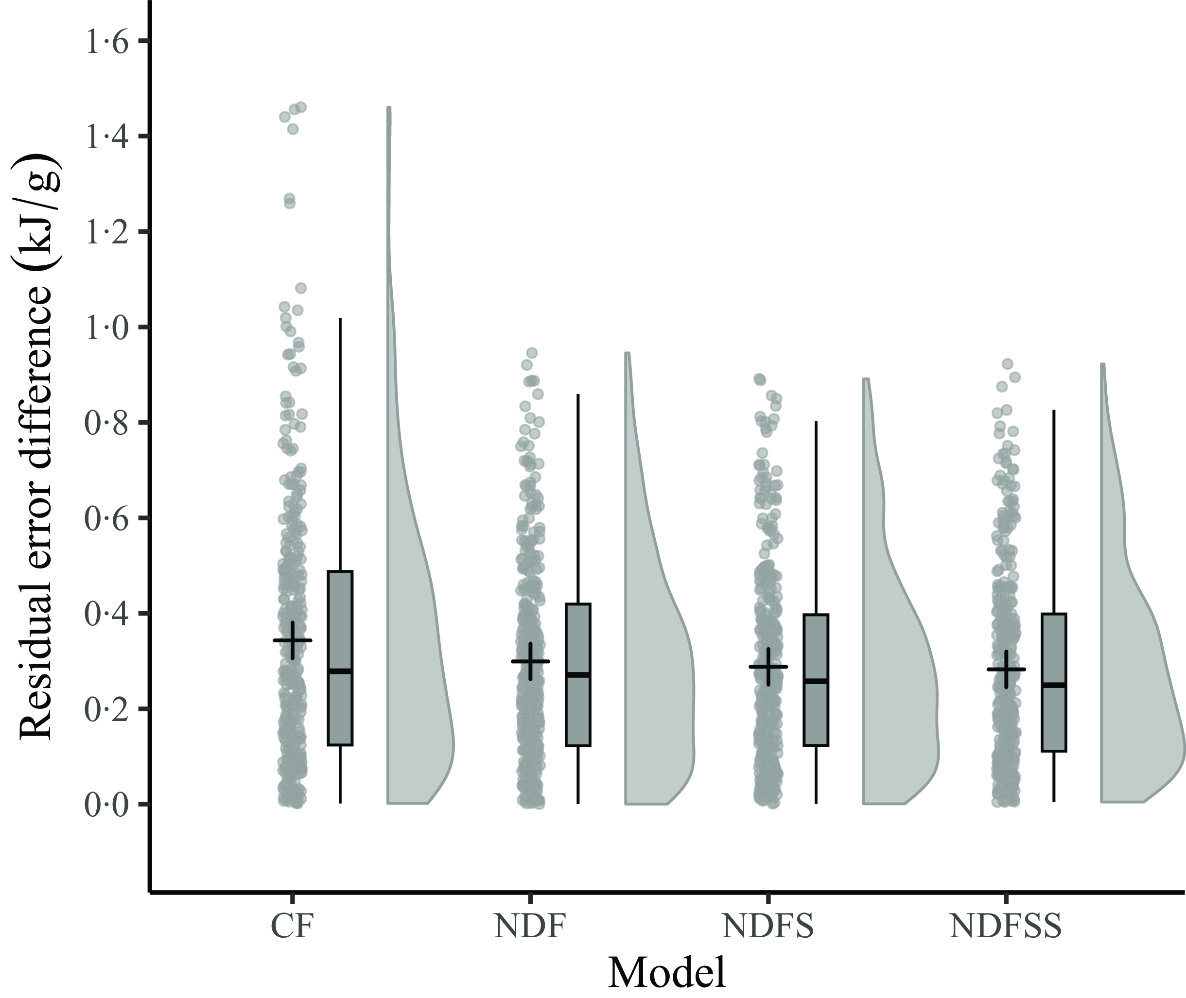
Since the mean actual and predicted ME densities of the four regression models using the common dataset are the same (14·43 kJ/g) and the average of the residuals zero, we compared the accuracy and precision of the four models by analysing the absolute residuals. Figure 4 shows the distribution of the absolute errors as a raincloud plot. A preliminary examination for normality with a Q-Q plot (not shown) and the Shapiro–Wilk test showed that the regressions’ absolute residuals were not normally distributed (W = 0·93, P < 0·001). Consequently, we used the non-parametric Kruskal–Wallis test, which showed that the overall difference between the regressions’ absolute residuals was not statistically significant at the 5 % level (P = 0·11). No further testing was deemed necessary. The InVivoStat Equivalence TOST test showed that the four sets of absolute residuals are equivalent at the 5 % level within ± 0·1 kJ/g. Thus, apart from the few outlying absolute residuals with the CF model, there seems to be little difference in the accuracy of the four regression models in predicting the ME density of individual records.
A raincloud plot of the residual error differences (actual minus predicted values) for the 359 records from the four regression models. The boxplot shows the median value and the interquartile range (25th–75th percentile). The cross is the mean of the data points. The vertical bars show the upper and lower outlier gates. Points outside the gates are considered outliers. CF, crude fibre; NDF, neutral detergent fibre; NDFS, neutral detergent fibre plus starch; NDFSS, neutral detergent fibre plus starch and sugars.
Finally, we obtained estimates of analysis costs for the analytes in the four regression models. Since these will change over time, we have expressed them relative to that of the CF model. The relative costs for the four analytical packages in 2023 were CF, 1; NDF, 1·4; NDFS, 1·9; and NDFSS, 2·2. Despite the higher costs, the improvement in MAE over the four models for the global and common data is less than 0·15 kJ/g, which is only about 1 % of the typical ME density.
The effectiveness of the four regression models in estimating metabolisable energy density in future datasets
Table 8 shows the 10-fold cross-validation data for the prediction of ME density in the four analytical models. The adjusted R 2, RSD, RMSE and MAE values indicate negligible overfitting since they are little different from the equivalent values in Table 4. This observation suggests that the regressions provided in this paper can accurately predict the ME density of additional future datasets, providing the new data’s nutrient levels and energy densities fall within the ranges shown in the descriptives. This assertion holds even if one takes the most unfavourable 95 % CI values. For example, in some future comparable datasets, the predictors in the CF model would typically account for about 75 % of the variation in the ME density prediction, and the MAE would be no more than ± 0·43 kJ/g. The improvement in prediction and GOF values from the CF to NDFSS datasets follows a similar pattern to the existing regressions. Thus, the three NDF-based regressions would improve predictive quality over CF, although the biological effect is small. The simpler predictive R 2 values were similar to those of the adjusted R 2.
The probable range of goodness-of-fit measures for metabolisable energy density on future datasets with similar characteristics to the diets in this study, determined by a 10-fold cross-validation analysis repeated ten times. Values in parenthesis are the 95 % CI

1The Predicted R 2 values from Table 4b have been included for comparison.
Comparison of regression equations with previously published ones
Although investigators have developed numerous regression equations to estimate ME density in pigs, many are based on only a few nutrients. We collated several regression equations developed to predict the ME density of pig diets using a more comprehensive range of nutrients similar to our selection (Table 9). The comparatively large intercept values in the ME-density intercept models make applying meaningful comparisons for the nutrient coefficients difficult. That issue is not a problem for those from the no-intercept models. While the CF coefficient is often negative, that is not axiomatic, though its value is close to zero. Each regression provides a similar predicted ME density when applied to the analytical data from the GF subset of the 359 ‘common records’ dataset. As one might expect, the GOF values on regressions based on a single laboratory are generally slightly better than those from this study. Morgan’s RSD/RMSE values are much higher, possibly because the regressions are based on the combined data from ingredients and complete diets. We return to this information in the Discussion.
Published equations for the prediction of metabolisable energy (ME) density from analytical components of diets standardised as g/100 g for nutrients and kJ/g for energy. The regression equations have been applied to the average nutrient values for the 271 grower/finisher records from the common dataset to give a predicted ME density. The average measured ME density of the 271 records was 14·34 kJ/g. For consistency, the predicted ME densities and goodness-of-fit indices have been rounded to two decimal places. See footnote 1 for the definition of the residues (Res1 to 4)
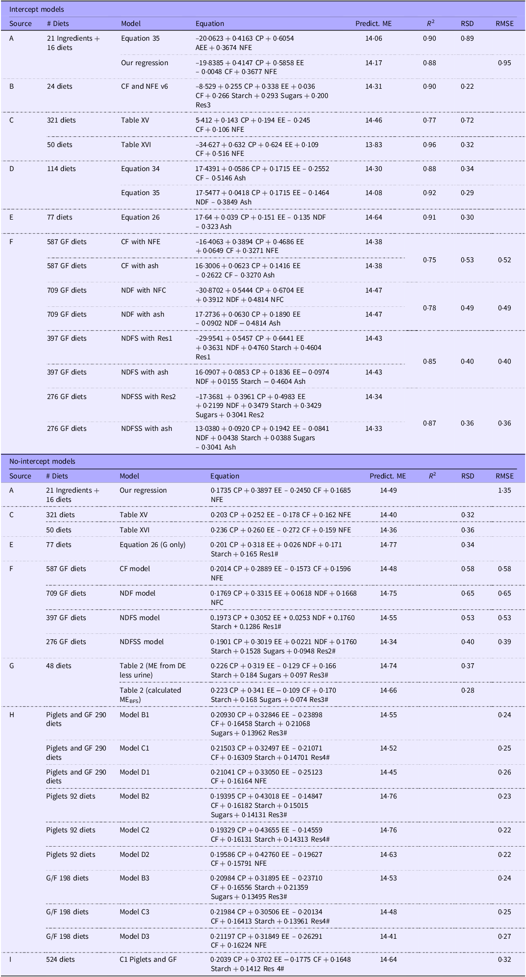
1# Organic residue definitions: Res1: 100-(CP + EE + NDF + Starch+Ash); Res2: 100-(CP + EE + NDF + Starch+Sugars+Ash); Res3: 100-(CP + EE + CF + Starch+Sugars+Ash); Res4: 100-(CP + EE + CF + Starch+Ash).
2Source key: (A) Morgan et al., 1975 II (see 3 below), (B) Eeckhout and Moermans, 1981, (C) Just et al., 1984, (D) Noblet and Perez 1993, (E) Le Goff and Noblet, 2001, (F) Current paper, (G) Kirchgessner and Roth, 1983, (H) Bulang and Rodehutscord 2009, (I) Grümpel-Schlüter et al., 2021.
3Mean analytical values (%, g/100 g) for the 271 G/F records in the common dataset: CP 18·50, EE 4·10, CF 5·29, NFE 65·17, NDF 15·55, NFC 54·91, Starch 46·15, Sugars 4·92, Res1 8·77, Res2 3·84, Res3 14·09, Res4 19·02, Ash 6·94.
4The Morgan data combine ingredient and diet data. Their original Eq 35 uses acid hydrolysis ether extract as a coefficient. We have used the ether extract value, which introduces a small error in the predicted ME value. We carried out a multiple regression analysis of Morgan’s data to estimate the coefficients of intercept and no-intercept models that included CP, EE, CF and NFE. Our regression based on CP, EE and NFE gave coefficients nearly identical to those of Morgan’s Eq 35 despite substituting EE for AEE.
5For our intercept-based regressions (F), the GOF values are from the combined GF and adult data.
6For reasons given in the text, R 2 values are not relevant for no-intercept models and are excluded even when given in a publication.
Discussion
We have developed a series of predictive equations for the ME density of murine diets from their nutrient analysis. There were insufficient suitable data from murine studies, and we relied on data from pig studies. As Fig. 1 shows, there is good agreement in digestibility between pigs and murine models above 0·65D, and several studies confirm that the similarity extends to metabolisability. Basing equations on pig data has major advantages. There is a large amount of published data from a wide range of laboratories, and the dietary nutrient levels and ingredients are those often seen in murine diets.
Variable selection was primarily dictated by analytical packages routinely reported by manufacturers for diets for laboratory rats and mice(Reference Tobin, Schuhmacher, Hau and Schapiro1). The most widely used is the proximate analysis, though NDF sometimes replaces CF since it is considered a better estimate of fibre. Although routine pig or murine diet analysis rarely includes starch and sugars, they were part of the analytical packages in many publications. We included them in our datasets and regression models to test if their inclusion in routine nutrient analysis might be beneficial in providing more accurate and reliable estimates of energy density and sufficiently so to warrant the additional cost.
With compositional data such as ours, where the values of potential predictors should total 100, dropping one predictor is often used to avoid multicollinearity(Reference Mason and Perreault59). We decided to choose between ash and a residue, such as NFE or NFC, based on the output from the correlation matrices, our desire to be consistent across the models and compatibility with other studies. There is no consistency in the literature (see, e.g. Table 9). One can choose between ash- or residue-based models from a statistical and biological perspective. While residue-based regressions tend to give more ‘physiologically meaningful’ coefficients(Reference Just, Jørgensen and Fernández22), they increase collinearity and result in higher VIF values for most coefficients. Although a high VIF may be associated with increased coefficient variance and imprecision, there is decreased risk with large sample numbers and high R 2 values(Reference Mason and Perreault59,Reference Grewal, Cote and Baumgartner65–Reference Das and Chatterjee68) . Our estimation of CVse in the ash- and residue-based regressions and P values confirmed no detrimental effect of collinearity on the precision of the coefficients. From a biological perspective, although ash could affect energy density by increasing the endogenous losses of protein and fat(Reference Selle, Ravindran and Cowieson69, Reference Stroebinger, Rutherfurd and Henare70), the evidence suggests that any effects are small or non-existent in pigs(Reference Jørgensen, Jakobsen and Eggum71, Reference Espinosa, Torres and Velayudhan72) but perhaps significant in poultry(Reference Cowieson, Ruckebusch and Sorbara73). We believe both ash- and residue-based regressions are satisfactory, and we include both since each has merits that are ultimately best assessed by the reader.
An equation generated from one data source may not apply more generally because of the many differences in the animals, environment and methodology used(Reference Noblet and Perez24). We sought to overcome this limitation by selecting data from numerous studies encompassing various pig breeds, diet preparations and types, nutrient levels, environmental conditions and technical practices. By analysing data from such a broad spectrum, we mitigate the risks of overfitting and shrinkage(Reference Yarkoni and Westfall56, Reference Babyak74) and improve reproducibility(Reference Voelkl, Vogt and Sena75), ensuring our models are more generalisable and reflective of real-world variability(Reference Hastie, Tibshirani and Friedman76). This approach significantly enhances the reliability of our predictive models when applied to future datasets. Choi(Reference Choi, Sung and Kim30), Sung(Reference Sung and Kim29) and their colleagues have taken a similar approach but with fewer samples and predictors and without equivalent prediction equations for dietary ME density.
This diverse background comes with a penalty, though we consider that the utilitarian nature of our regressions outweighs the disadvantages. The primary ‘disadvantage’ is that these other variable background factors increase the unattributed variation, resulting, for example, in slightly poorer adjusted R 2, RSD and MAE values than one might hope. Nevertheless, the adjusted R 2 values are still good, ranging from 0·75 to 0·87 for the four models(Reference Gupta, Stead and Ganti60). The typical RSD from carefully conducted, single-site studies by Noblet is about 0·34 kJ ME/g for a CF regression and about 0·30 kJ ME/g for the NDF one (Table 9). In our ‘global’ equations, the values were higher at 0·52 and 0·46 kJ/g for the CF and NDF models. When we restricted the data to 359 sets common to all models and from fewer sources, the RSD values were about midway between the single site and ‘global’ models, at 0·45 and 0·37 kJ/g, respectively. Two related studies by Bulang and Rodehutscord(Reference Bulang and Rodehutscord63) and Grümpel-Schlüter and colleagues(Reference Grümpel-Schlüter, Berk and Schäffler64) deviate from our expectations and produce unusually low RMSE values (median c. 0·25 kJ/g) despite a diverse data source. The divergence may result from calculating each diet’s ME density from an equation recommended by the GfE(19,20) rather than measurement. This approach inevitably decreases variation.
Investigators have used intercept and non-intercept regressions to predict energy density from dietary chemical constituents (Table 9). Removal of the intercept slightly decreases accuracy, as can be seen when comparing the values predicted with Noblet’s (E) and our data (F) in Table 9 by the two regression types. The GOF was similar in both regression types.
The no-intercept models have some advantages: they avoid the issue of ash- or residue-based regressions discussed above, and unlike those in the intercept models, one can apply their coefficients to diets and ingredients alike(Reference Noblet, Wu and Choct43). Moreover, excluding intercepts, which are large contributors to the dependent variable, may provide ‘physiologically relevant’ coefficients(Reference Just, Jørgensen and Fernández22) that may appeal to some investigators. We use both forms of regression, with the intercept model providing the definitive prediction and the no-intercept model providing a (net) measure of the contribution of the energy-yielding nutrients to the total energy density(Reference Noblet, Wu and Choct43).
The intercepts and nutrient coefficients in Table 2 apply to both GF and AD animals. Adding a growth phase to the regressions is a powerful feature and accommodates data consolidation from the GF and AD animals in the regression. It defines the additional energy that should be added to the dependent variable for AD animals to reflect their greater energy absorption and metabolisability(Reference Le Goff and Noblet62, Reference Lowell, Liu and Stein77, Reference Noblet and Shi78). However, the ages of animals in most murine research and regulatory studies are probably best represented by GF pigs and the base prediction equations, even though the age effect may exist in older murine models(Reference Itoh, Kaneko and Ohshima79). Determining the effect of the growth phase on predicted ME density is only possible with the intercept models.
Though it is unlikely one would predict GE density from nutrient analyses, we have included GE density regressions here as a test of the regression process’s effectiveness when applied to ME density predictions. Since the GE coefficients in the four models are affected by the intercept size, the best comparison is with the no-intercept regressions in Table 5a. Across the models, there is good agreement with the published values for simple analytes such as CP, EE, starch and sucrose (Table 3) from the residue-based regressions, though not those based on ash. Assessing the accuracy of GE density coefficients for CF or NDF is more complex. Their energy content depends on their fibre composition, which varies with the ingredient(Reference Mongeau and Brassard80–Reference Knudsen86). Cellulose and hemicellulose, two of the main components in fibre, have values of about 16–18 kJ/g, while lignin ranges from 21 to 30 kJ/g(Reference Kaltschmitt, Hartmann and Hofbauer87–Reference Kienzle, Schrag and Butterwick91). Fibre may also include small amounts of protein (c.23–24 kJ/g).
Although obtaining reliable estimates of the GE density of nutrients from regressions is reassuring despite the empirical nature of the regressions, the study’s primary purpose was to predict ME density. In contrast to the nutrient coefficients for GE density, there is considerable variation in comparable coefficients in this study’s four ME density models and other published equations (Table 9). The exceptionally high intercept values contribute to much of the variation, especially in those regressions that include residues (NFE, NFC, Res1 or Res2). Overall, there is no correspondence in the intercept regressions between theoretical ME density values and those obtained from the coefficients. Nevertheless, despite a large variation in intercept and coefficient values between models, the different regression equations generally give predicted ME density values close to the actual values.
The no-intercept regressions allow the comparison of regression-derived nutrient coefficients, unaffected by the large and variable intercepts, with our theoretical estimates for ME density (Table 3). The fibre regression coefficients are much lower than calculated ME densities (CF, c.300 % lower, and NDF 65 % lower). In contrast, those for protein and EE are about 10–20 % higher. These results are consistent since dietary fibre is known to increase energy loss from protein and fat(Reference Agyekum and Nyachoti92–Reference Zhang, de Vries and Gerrits94), and the nature of the regression analysis allocates these losses to fibre rather than the protein and EE coefficients. There is a good agreement for the soluble carbohydrates (0–5 % difference) consistent with the absence of a significant effect of fibre on starch absorption(Reference Agyekum and Nyachoti92,Reference Wilfart, Montagne and Simmins95,Reference Just96) .
The GOF values showed that our regression models were consistently good and improved with the increasing characterisation of the diet’s nutrient composition. The GOF measurements were inevitably poorer with the ME density regressions than those for GE density, reflecting increased experimental variation and errors associated with biological studies. Internal validation based on predicted R 2 and k-fold GOF measurements confirms that our regression equations explain existing relationships between energy density and the chemical analytes well and are suitable for future predictions without exhibiting overfitting. We are confident that the first three models provide generalised predictions suitable for widespread practical use. However, data from the Noblet group(Reference Noblet and Perez24,Reference Noblet, Fortune and Dupire39,Reference Le Goff and Noblet62,Reference Shi and Noblet97) dominated the NDFSS model, contributing about 87 % of the records. This may lead to some overfitting, though less than using data from a single study.
Although GOF indices such as RMSE, RSD or MAE reflect errors in the regression model, they apply to populations rather than individual samples. While this expression of error may be suitable for a diet manufacturer providing an illustrative ME density as a guideline, most investigators should be concerned with the prediction error in a single diet sample rather than that averaged over a population of samples. Here, the PI is the best estimate of uncertainty when new predicted values are required. Unfortunately, investigators often ignore the effect of the PI on a study. As with the MAE, PI improves across the four models but only by about 0·3 kJ/g. One should assume the PI could be up to ± 1 kJ/g of the predicted value.
External validation of prediction equations is important, although often overlooked. Its significance is particularly well-recognised in clinical studies(Reference Steyerberg98). We achieved some benefits of external validation by comparing the actual ME density of a test diet with values predicted from our equations and other published equations (Table 9). While this step does not replace traditional external validation, it still reinforces the validity of the equations. There was good agreement, though it was slightly better for the intercept than the no-intercept model.
In selecting the best regression model for routine use, one should consider the analysis’s complexity, cost and GOF. We found no evidence from either the Kruskal–Wallis or equivalence testing that any of the four analytical models was better at predicting ME density. However, there was a slight improvement in GOF values with greater complexity. The CF model seems adequate for murine models, especially since murine laboratory diet analysis commonly includes the necessary predictors. Although NDF-based models improve the prediction error, they cost up to twice that of the CF model analysis. For some studies, these increases in cost for such little gain might be cost-effective, though unlikely.
There are three constraints to using our equations. First, although diet manufacturers provide typical nutrient estimates, we recommend the investigator obtain chemical analysis data on the diet used for optimal accuracy. Second, the regressions may not apply to purified diets for which the Atwater factors remain relevant(Reference Bielohuby, Bodendorf and Brandstetter11). Third, their accuracy may decline with very high or low levels of individual nutrients, though such values would be uncommon for murine diets (or complete diets for pigs).
In developing our regressions, we have accumulated more data records than in previous publications and subjected them to rigorous statistical analysis. Possibly, for the first time, we have compared the relative merits of predictions based on several analytical packages in a single study and evaluated their cost-effectiveness. We have also provided realistic estimates of the possible prediction error when applied to diet samples or an individual batch. Our inability to validate these predictive equations with murine data remains a weakness and indicates the need for further reliable ME density measurements in rats and mice. We know of only one study that examined the application of a pig equation to natural-ingredient murine diets to predict ME density. Bielohuby and colleagues(Reference Bielohuby, Bodendorf and Brandstetter11) found the equation (unattributed, but Kirchgessner and Roth’s MEBFS equation(Reference Kirchgessner and Roth25) shown in Table 9) was more accurate than Atwater factors for natural-ingredient rat diets. However, the eleven diets tested are too few to validate their use confidently.
Although near-infrared spectroscopy has been suggested as an alternative to predict dietary energy density, it is not straightforward. It is easily affected by small environmental and sample changes and may require several hundred calibration samples, and the equipment is expensive(Reference Maduro Dias, Nunes and Borba99). Nor do we consider its accuracy for energy density predictions better than ours (cf Noel and colleagues(Reference Noel, Jørgensen and Knudsen100)).
Although several previous studies (Table 9) predict the ME density of pig diets from chemical analysis, this study provides more robust validated prediction equations, with standard combinations of the most common feed analytes as predictors. Several of the studies use only calculated ME density and no-intercept models. The regressions are from single laboratories, include fewer records and inevitably underestimate prediction errors when used widely. We used more extensive measures of GOF and validation to ensure that the regressions would maintain their robustness when applied to new data. All four regression models give good GE and ME density predictions that can be applied to murine diets. While the quality of fit to the data improves slightly with increased numbers or refinement of predictors, analysis costs increase substantially. Moreover, the differences in prediction errors are small relative to the predicted values. Thus, the CF equation seems an adequate practical approach to determining ME density. If one requires higher precision and accuracy than shown here, one must measure ME density in vivo.
Supplementary material
For supplementary material/s referred to in this article, please visit https://doi.org/10.1017/S0007114525000042.
Acknowledgements
We are grateful for further analytical data from Jean Noblet and his comments on our approach to the study. Many other investigators also provided helpful comments and expanded on their published data, particularly Su Lee and Brian Kerr. Finally, GT wishes to thank the staff of the Oxford University libraries, particularly for their efforts to maintain service during the COVID-19 pandemic.
This research received no specific grant from any funding agency, commercial or not-for-profit sectors. A. S. is employed by ssniff Spezialdiaeten but has received no direct payments to support this study.
G. T. – study design, data collection, statistical analysis, manuscript preparation. A. S. – study design, manuscript preparation and review. T. G. and Ł. S. – guidance on statistical analysis and using the R programming language, manuscript review.
There are no conflicts of interest.
There are no ethical issues in this study.