


1. Introduction
Rapidly rotating contained flows subjected to low-amplitude parametric forcing, such as libration or precession modulating the rotation amplitude or direction, are ubiquitous in geophysical and astrophysical flows, as well as in many technological applications. Rapidly rotating flows, characterized by small Ekman numbers ( $ {\textit {E}} \ll 1$, the ratio of rotation time scale to viscous time scale), support inertial waves due to the restorative Coriolis force. Low-amplitude (Rossby numbers $\epsilon \ll 1$) parametric forcing can extract a portion of the available rotational energy in a rapidly rotating contained body of fluid and convert it into intense fluid motions via the resonant excitation of inertial waves (Malkus Reference Malkus1968). The Ekman numbers of geophysical and astrophysical flows are many orders of magnitude smaller than those attainable in laboratory experiments, and the forcing amplitudes in experiments need to be relatively large in order to measure a signal reliably (Le Bars et al. Reference Le Bars, Barik, Burmann, Lathrop, Noir, Schaeffer and Triana2022). The response flows are then dominated by viscous and nonlinear effects that may not be prevalent in very low Ekman number and low forcing amplitude regimes. Direct numerical simulations of the Navier–Stokes equations with no-slip boundary conditions can now simulate librating and precessing flows at Ekman numbers as small as, or smaller than, those in laboratory experiments, at small forcing amplitudes over the entire inertial range of forcing frequencies. This is opening up new insights into these fascinating flows.
The inertial waves that are supported in rapidly rotating flows have quite peculiar properties, in part due to the anisotropy imposed by the background rotation. In the inviscid linear regime, their dispersion relation relates their orientation relative to the rotation axis solely with their frequency,  $(\hat {\boldsymbol {\xi }}\boldsymbol {\cdot}\hat {\boldsymbol {k}})^2=\omega ^2$, where $\hat {\boldsymbol {\xi }}$ is the unit vector of the background rotation, $\hat {\boldsymbol {k}}$ is the inertial wave unit vector and $\omega$ is the wave's frequency scaled by twice the background rotation. They are transverse waves with their group velocity orthogonal to their wave vector. In the linear inviscid regime, the governing equations are hyperbolic in the spatial variables, and the group velocity directions coincide with the characteristics. The dispersion relation leads to peculiar behaviour upon reflections at solid walls (Phillips Reference Phillips1963); the incident and reflected waves have the same frequency irrespective of the wall orientation, but the relation between incident and reflected wave vectors does depend on the wall orientation. Focusing or defocusing (increase or decrease in the wavenumber and energy upon reflection) depends on whether the reflection is super or subcritical. Criticality is determined by the ratio of the cosines of angles between the rotation axis and the wall normal, $\hat {\boldsymbol {n}}$, and the rotation axis and wave vector, $\lambda =(\hat {\boldsymbol {\xi }}\boldsymbol {\cdot}\hat {\boldsymbol {n}})/ (\hat {\boldsymbol {\xi }}\boldsymbol {\cdot}\hat {\boldsymbol {k}})$; the reflection is subcritical if $|\lambda | < 1$, supercritical if $|\lambda | > 1$ and critical if $|\lambda |=1$. As noted by Phillips (Reference Phillips1963), the inviscid considerations of how inertial waves reflect on walls become complicated for critical reflections. The reflected wave is ‘trapped’ in the wall, and for small $ {\textit {E}}$ the interaction with the viscous boundary layer is non-negligible, as are the nonlinearities which lead to a significant mean flow (Riley Reference Riley2001). Analogous effects were considered for the critical reflections of internal waves in a stratified system (Cacchione & Wunsch Reference Cacchione and Wunsch1974); linear inviscid theory predicts infinite velocities along the wall inclined at the critical angle, while experiments show that at the critical angle, the strong shearing motion becomes unstable, forms a series of vortices that overturn, mix fluid and propagate into the interior.
While the effects of a critical slope in stratified systems have attracted extensive attention (e.g. Gordon Reference Gordon1980; Thorpe Reference Thorpe1997; Slinn & Riley Reference Slinn and Riley1998; Dauxois & Young Reference Dauxois and Young1999; Javam, Imberger & Armfield Reference Javam, Imberger and Armfield1999; Scotti Reference Scotti2011; Horne et al. Reference Horne, Schmitt, Pustelnik, Joubaud and Odier2021), the situation in rotating systems has not been as systematically studied. This is in part due to internal waves lending themselves to being studied in planar two-dimensional systems, whereas inertial waves in rotating systems are intrinsically helical, with velocity and vorticity vectors parallel and in phase (Davidson Reference Davidson2013), and as such cannot be described in a planar two-dimensional setting (in which velocity and vorticity are orthogonal). Axisymmetric rotating flows have three-component velocity fields that depend only on two spatial directions, and in axisymmetric containers, such as a spherical shell, the analysis of boundary-layer eruptions at critical latitudes (points where  $|\lambda |=1$) is tractable. Kerswell (Reference Kerswell1995) showed that for small $ {\textit {E}}$ and small libration forcing amplitudes $\epsilon$, the oscillatory Ekman layer erupts at critical latitudes spawning shear layers into the bulk of the fluid.
Rotating systems subjected to libration have also been studied in relatively long rectangular containers with a trapezoidal cross-section (Maas Reference Maas2001). In this type of geometry, the entire wall of the container that is at an oblique angle to the rotation axis has a critical slope for a given forcing frequency (in contrast to only a line on the sphere at the critical latitude). As well as experiments, this librating geometry has also been studied theoretically using linear inviscid ray tracing (e.g. Manders & Maas Reference Manders and Maas2003; Pillet, Maas & Dauxois Reference Pillet, Maas and Dauxois2019). Those studies focused primarily on the wave attractors in the bulk flow, but also considered the critical slope attractor, where for a particular forcing frequency the slope of the inclined wall is critical and a branch of the wave attractor becomes trapped in the wall, while other branches of the attractor continue to reside in the bulk. The linear inviscid analysis, however, is inadequate in describing the ensuing hydrodynamics.
For a cube rotating about an axis through two diagonally opposite vertices, all walls have critical slope for libration frequency corresponding to  $\omega ^2=1/3$ (Wu, Welfert & Lopez Reference Wu, Welfert and Lopez2020). All relative flow is trapped in the wall boundary layers, and the interior flow is essentially zero for sufficiently small Rossby numbers $\epsilon$. The response flow is a periodic travelling wave completely constrained within the boundary layers, referred to as a boundary-confined wave. This wave was first observed in the librating cube using a second-order in time spectral-collocation technique to solve the Navier–Stokes equations (Wu et al. Reference Wu, Welfert and Lopez2020). Well-resolved solutions were obtained for Ekman numbers as small as $ {\textit {E}}=10^{-7}$. Here, we re-examine the $\omega ^2=1/3$ case using a third-order in time scheme with a spectral-Galerkin method in space (Wu, Huang & Shen Reference Wu, Huang and Shen2022). All of the prior results were faithfully reproduced with the new numerical code using far fewer time steps per forcing period. For small forcing amplitudes, $\epsilon = {\textit {E}}$, we determine how the boundary-layer thickness and the enstrophy density in the wall boundary layers scale with $ {\textit {E}}$ over several decades. Furthermore, the much improved numerical conditioning of the new code enables us to examine the hydrodynamic instabilities that ensue as the libration amplitude (Rossby number) is increased beyond $\epsilon \sim {O}( {\textit {E}}^{1/2})$.
2. Governing equations and their numerical solutions
A cube of side length  $L$ is completely filled with an incompressible fluid of kinematic viscosity $\nu$. Using $L$ as the length scale, we introduce a non-dimensional Cartesian coordinate system $\boldsymbol {x}=(x,y,z)\in [-0.5,0.5]^3$ that is fixed to the cube with its origin at the cube centre. The cube is rotating about an axis in the direction $\hat {\boldsymbol {\xi }}=(1,1,1)/\sqrt {3}$, which passes through two diagonally opposite vertices of the cube (the north and south poles). The rotation is periodically modulated about a mean $\varOmega$, with modulation frequency $\sigma$ and modulation amplitude $\Delta \varOmega$. Using $1/\varOmega$ as the time scale, the non-dimensional velocity in the frame of reference of the librating cube is $\boldsymbol {u}$ and the non-dimensional angular velocity of the cube is
 \begin{equation} \boldsymbol{\varOmega}(t)=[1+\epsilon\cos(2\omega t)]\hat{\boldsymbol{\xi}}, \end{equation}
where  $\omega =\sigma /2\varOmega$ is the non-dimensional libration half-frequency and $\epsilon =\Delta \varOmega /\varOmega$ is the non-dimensional amplitude (Rossby number). Figure 1 shows a schematic of the librating cube.
Schematics of the librating cube, showing the coordinate system, the north and south poles, and the equatorial and meridional planes.

The system is governed by the Navier–Stokes equations. The reference frame of the librating cube introduces both a Coriolis force and an Euler force. In this frame, the no-slip boundary conditions are  $\boldsymbol {u}=\boldsymbol {0}$ on all walls of the cube. The non-dimensional governing equations in the librating frame are
 \begin{equation} \frac{\partial \boldsymbol{u}}{\partial t} +(\boldsymbol{u}\boldsymbol{\cdot}\boldsymbol{\nabla})\boldsymbol{u} +2\boldsymbol{\varOmega} \times \boldsymbol{u} +\boldsymbol{\nabla}p -{\textit{E}}\nabla^2\boldsymbol{u} ={-}\frac{{\rm d}\boldsymbol{\varOmega}}{{\rm d}t} \times \boldsymbol{x}, \quad \boldsymbol{\nabla}\boldsymbol{\cdot}\boldsymbol{u}=0, \end{equation}
where  $ {\textit {E}}=\nu /(\varOmega L^2)$ is the Ekman number and $p$ is the reduced pressure, incorporating the centrifugal force. In our earlier study of this system (Wu et al. Reference Wu, Welfert and Lopez2020), it was found that the magnitude of the response flow velocity scaled linearly with the forcing amplitude, $\|\boldsymbol {u}\|\propto \epsilon$, for $\epsilon \lesssim {O}( {\textit {E}}^{1/2})$. In order to consider the small $\epsilon$ and small $ {\textit {E}}$ regimes, it is convenient to rescale the velocity as $\boldsymbol {v}=\epsilon ^{-1}\boldsymbol {u}$, in which case the governing equations become
 \begin{equation} \frac{\partial \boldsymbol{v}}{\partial t} +\epsilon(\boldsymbol{v}\boldsymbol{\cdot}\boldsymbol{\nabla})\boldsymbol{v} +2\boldsymbol{\varOmega} \times \boldsymbol{v} +\boldsymbol{\nabla}q -{\textit{E}}\nabla^2\boldsymbol{v} =2\omega\sin(2\omega t)\,\hat{\boldsymbol{\xi}}\times \boldsymbol{x}, \quad \boldsymbol{\nabla}\boldsymbol{\cdot}\boldsymbol{v}=0, \end{equation}
where  $q$ is the corresponding scaled pressure. In this formulation, the response flow, $\boldsymbol {v}$, remains of ${O}(1)$ as $\epsilon \to 0$, the nonlinear advection terms have a factor of $\epsilon$, the viscous terms have a factor of $ {\textit {E}}$, and the librational forcing term on the right-hand side remains of ${O}(1)$ even as $\epsilon \to 0$. There is also an $\epsilon$ contribution in the unsteady Coriolis term due to $\boldsymbol {\varOmega }(t)$ (2.1).
The system of governing equations (2.3) is first discretized using a third-order consistent splitting scheme for the Navier–Stokes equations with the Coriolis and Euler forces and the viscous terms treated implicitly. This leads to a coupled elliptic equation with variable coefficients for the velocity and a Poisson equation with constant coefficients for the pressure at each time step. These equations are then discretized in  $(x,y,z)$-space using a Legendre–Galerkin spectral approach with Legendre polynomials of degree $m$ in each direction for each of the three velocity components and $m-\!2$ for the pressure. This leads to a better-conditioned symmetric positive definite banded system than the non-symmetric linear system resulting from the pseudo-spectral-collocation approach previously used (Wu et al. Reference Wu, Welfert and Lopez2020). The degree $m$ of the Legendre polynomials used ranges from $m=50$ for the largest Ekman numbers considered to $m=250$ for $ {\textit {E}}=10^{-7}$ and $\epsilon \sim {O}( {\textit {E}}^{1/2})$. The resulting discretized system requires the solution of coupled linear systems with variable coefficients at each time step, which are solved using diagonalization. For all Ekman numbers $ {\textit {E}}$, the number of time steps per forcing period used was 200 for small $\epsilon$. As $\epsilon \to {\textit {E}}^{1/2}$, the system becomes susceptible to hydrodynamic instabilities requiring finer temporal resolution (up to $800$ time steps per libration period). Details of the method, stability analysis and accuracy tests on rotating flows, including that studied here, are presented in Wu et al. (Reference Wu, Huang and Shen2022).
The governing equations and boundary conditions are invariant to  $\mathcal {R}$, a discrete $2{\rm \pi} /3$ rotation symmetry with respect to the rotation axis $\hat {\boldsymbol {\xi }}$, and a centrosymmetry $\mathcal {C}$ with respect to the coordinate origin. The centrosymmetry $\mathcal {C}$ generates a $Z_{2}$ cyclic group and the rotation symmetry $\mathcal {R}$ generates a $Z_{3}$ cyclic group. These two symmetries commute, i.e. $\mathcal {C}\mathcal {R}=\mathcal {R}\mathcal {C}$, and their combination defines the resultant spatial symmetry of the system $\mathcal {X}=\mathcal {C}\mathcal {R}=\mathcal {R}\mathcal {C}$, that generates a $Z_{6}$ cyclic group whose action on the velocity $\boldsymbol {v}=(u,v,w)$ is
 \begin{equation} {\mathcal{X}}:[u,v,w](x,y,z,t) \mapsto [{-}w,-u,-v]({-}z,-x,-y). \end{equation}
Due to the librational forcing, of period  $\tau ={\rm \pi} /\omega$, the governing equations and boundary conditions are also invariant to the discrete time translation symmetry $t\to t+\tau$. A measure of the flow's departure from being $\mathcal {X}$ invariant is
 \begin{equation} S={\|\boldsymbol{v}-\mathcal{X}\boldsymbol{v}\|^2}/{\|\boldsymbol{v}\|^2}, \end{equation}
where
 \begin{equation} \|\boldsymbol{v}\|^2=\int_{{-}0.5}^{0.5}\int_{{-}0.5}^{0.5}\int_{{-}0.5}^{0.5} (u^2+v^2+w^2) \,{{\rm d}\kern0.06em x}\,{{\rm d} y}\,{\rm d}z. \end{equation}
3. Boundary-confined waves
The oscillatory boundary layers on the librating cube walls were found to be of uniform thickness for  $\omega ^2=1/3$ (see figure 12 of Wu et al. Reference Wu, Welfert and Lopez2020), although the enstrophy density, $\mathcal {E}=|\boldsymbol {\nabla }\times \boldsymbol {v}|^2$, has considerable spatio-temporal variations on the walls. We begin by examining the boundary layer at a point in the middle of a wall (due to symmetry, the middle of each of the six walls is identical), over several decades in $ {\textit {E}}$, examining the profiles of the enstrophy density along the wall-normal $x$-axis. The middle of a wall is chosen as it is the point on the wall furthest away from all edges and vertices. For $\omega ^2\sim 1/3$, wave beams are emitted from and converge to various edges and vertices (see Wu et al. Reference Wu, Welfert and Lopez2020, for details), and for exactly $\omega ^2=1/3$ in the linear inviscid idealization $ {\textit {E}}=\epsilon =0$, all flow is in a zero-thickness skin on the walls, in a delta-function-like distribution. How this distribution is approached as $ {\textit {E}}\to 0$ is now addressed. Note that for $\epsilon$ below some $ {\textit {E}}$-dependent critical value, the flow $\boldsymbol {v}$ is essentially independent of $\epsilon$. In order to ensure that $\epsilon$ remains below critical, we determine the boundary-layer structure using $\epsilon = {\textit {E}}$.
Figure 2 summarizes the boundary-layer structure for  $10^{-7}\le {\textit {E}}\le 10^{-4}$. Flows at larger $ {\textit {E}}$ are too viscous, lacking a proper boundary layer as the wall flow extends all the way to the centre of the cube. Even though the forcing amplitude $\epsilon$ is very small, there is a large mean flow, and so the profiles are presented as the time-average $\overline {\mathcal {E}}$, and the standard deviation (a measure of the oscillation amplitude) $\mathcal {E}_{SD}$, of the enstrophy density profiles along the line. For $ {\textit {E}}\lesssim 10^{-4}$, there are self-similar scalings, with the boundary-layer thickness for the time average scaling with $ {\textit {E}}^{1/3}$, whereas the boundary-layer thickness for the standard deviation becomes thinner faster with decreasing $ {\textit {E}}$, scaling with $ {\textit {E}}^{1/2}$. On the other hand, the magnitude of the time-averaged enstrophy density grows at a faster rate with decreasing $ {\textit {E}}$, scaling with $ {\textit {E}}^{-1.28}$, than the standard deviation does, which scales as $ {\textit {E}}^{-1.18}$, although these rates are not too dissimilar. In summary, as $ {\textit {E}}\to 0$ the time-averaged enstrophy density grows faster than its standard deviation, and the oscillations become restricted to a thinner wall region faster than the time-averaged enstrophy density does.
Profiles of the time average and standard deviation of the enstrophy density,  $\overline {\mathcal {E}}$ and $\mathcal {E}_{SD}$, along the $x$-axis, at various $ {\textit {E}}=\epsilon$ as indicated.

Using the above boundary-layer scalings, figure 3 shows snapshots on the cube walls of the enstrophy density,  $\mathcal {E}$, at the quarter phase of the libration, the time-averaged enstrophy $\overline {\mathcal {E}}$, and the fluctuation enstrophy, $\widetilde {\mathcal {E}}=\mathcal {E}-\overline {\mathcal {E}}$, also at the quarter phase. The colourmaps used to plot $\mathcal {E}$ and $\overline {\mathcal {E}}$ are scaled with $ {\textit {E}}^{1.28}$, whereas $\widetilde {\mathcal {E}}$, whose amplitude is related to the standard deviation $\mathcal {E}_{SD}$, is scaled with $ {\textit {E}}^{1.18}$. The supplementary movie 1 animates $\mathcal {E}$ and $\widetilde {\mathcal {E}}$ over one libration period. The orientation of the cube in these images has the rotation axis pointing out of the page, and the vertex at the centre is the north pole. The $\mathcal {E}$ animation shows large amplitude oscillations, primarily near the equatorial edges of the cube (i.e. the edges not connected to either the north or south pole), with the region of large oscillations diminishing with decreasing $ {\textit {E}}$. The regions with the largest $\overline {\mathcal {E}}$ are coincident with these. On the other hand, the animations of $\widetilde {\mathcal {E}}$ show a very regular wavy oscillation emitted from alternating equatorial edges and propagating to the north pole (by symmetry, a similar wavy oscillation is emitted from the other alternating equatorial edges and propagates to the south pole). The structure of this wave is independent of $ {\textit {E}}$ for $ {\textit {E}}\lesssim 10^{-4}$, and its amplitude has the same scaling as $\mathcal {E}_{SD}$. This wave is, in essence, the boundary-confined wave.
Snapshots on the surface of the cube librating with  $\omega =0.580$ at $ {\textit {E}}=\epsilon$, as indicated, of (a) the enstrophy density, $\mathcal {E}$, at the quarter phase of the libration, (b) the time-averaged enstrophy, $\overline {\mathcal {E}}$, and (c) the fluctuation enstrophy, $\widetilde {\mathcal {E}}=\mathcal {E}-\overline {\mathcal {E}}$, at the quarter phase. The orientation has the rotation axis pointing out of the page and the vertex in the middle is the north pole. Supplementary movie 1 available at https://doi.org/10.1017/jfm.2022.934 animates $\mathcal {E}$ and $\widetilde {\mathcal {E}}$ over one libration period.

All of the results for the boundary-confined wave presented so far are for very small forcing amplitudes,  $\epsilon = {\textit {E}}$. We now address how the flow depends on $\epsilon$. We do this for $ {\textit {E}}=10^{-5}$ as this $ {\textit {E}}$ is small enough to be representative of the small $ {\textit {E}}$ flows, but requires less computational resources compared with smaller $ {\textit {E}}$. As is suggested from the governing equations (2.3), increasing $\epsilon$ while keeping all other governing parameters fixed enhances the impact of the quadratic nonlinear advection term. This results in the periodic response flow $\boldsymbol {v}$ becoming less harmonic, giving rise to a time-averaged flow $\bar {\boldsymbol {v}}$ that grows with increasing $\epsilon$, whereas $\boldsymbol {v}$ is essentially independent of $\epsilon$ for $\epsilon$ not too large. Note that $\boldsymbol {u}=\epsilon \boldsymbol {v}\propto \epsilon$, $\bar {\boldsymbol {u}}=\epsilon \bar {\boldsymbol {v}}\propto \epsilon ^2$, and $\bar {\boldsymbol {v}}\propto \epsilon$. This is a general result for periodically forced flows; see Rubio, Lopez & Marques (Reference Rubio, Lopez and Marques2009, § 4.2) for a general discussion of how the temporal Fourier coefficients of a time-periodic solution scale with amplitude. The temporal harmonics of $\boldsymbol {v}$ at $\omega ^2=1/3$ correspond to frequencies beyond the inertial range, and so do not contribute directly to any inertial wave activity, but they do make the periodic response less harmonic.
Figure 4 shows profiles of the time-averaged enstrophy  $\overline {\mathcal {E}}(\boldsymbol {v})$, the corresponding standard deviation $\mathcal {E}_{SD}(\boldsymbol {v})$ and the (scaled) enstrophy of the time-averaged velocity $\mathcal {E}(\bar {\boldsymbol {v}})$ along the $x$-axis, for $ {\textit {E}}=10^{-5}$ and $10^{-5}\le \epsilon \le 0.03$. The $\overline {\mathcal {E}}(\boldsymbol {v})$ profiles are essentially identical for all $\epsilon \lesssim 0.01$; the profiles of the two larger $\epsilon =0.02$ and 0.03 have a very slight increase at $x\approx -0.1$. The standard deviation at the wall ( $x=-0.5$) is invariant to $\epsilon$, but its local maximum near the wall at $x\approx -0.47$ increases with increasing $\epsilon$ for $\epsilon >10^{-3}$. On the other hand, the profiles of $\mathcal {E}(\bar {\boldsymbol {v}})$ have a strong dependence on $\epsilon$. For the most part, these profiles collapse with the expected scaling $\mathcal {E}(\bar {\boldsymbol {v}})\propto \epsilon ^2$, in particular for the local maximum at $x\approx -0.47$. This scaling is less successful away from the wall, but the scaled profiles only vary by approximately one order of magnitude for almost four orders of magnitude variation in $\epsilon$.
Profiles along the  $x$-axis of (a) the time-averaged enstrophy $\overline {\mathcal {E}}(\boldsymbol {v})$, (b) the corresponding standard deviation $\mathcal {E}_{SD}(\boldsymbol {v})$ and (c) the scaled enstrophy of the time-averaged velocity $\epsilon ^{-2}\mathcal {E}(\bar {\boldsymbol {v}})$, for $ {\textit {E}}=10^{-5}$ and $\epsilon$ as indicated.

To further explore how the effects of the mean flow manifest, figure 5 shows plots of the time-averaged enstrophy,  $\overline {\mathcal {E}}(\boldsymbol {v})$, the corresponding standard deviation, $\mathcal {E}_{SD}(\boldsymbol {v})$, and the scaled enstrophy of the time-averaged flow, $\epsilon ^{-2}\mathcal {E}(\bar {\boldsymbol {v}})$, in the equatorial and meridional planes for $ {\textit {E}}=10^{-5}$ over wide range of $\epsilon$. The supplementary movie 2 animates $\mathcal {E}(\boldsymbol {v})$ over a libration period. The boundary-layer structure (both thickness and intensity) is essentially independent of $\epsilon$ and over the entire libration period for $\epsilon \lesssim 0.01$, the boundary layer is virtually indistinguishable from its time average, shown in figure 5(a). Exceptions to this are in the corners of the equatorial plane (which correspond to the midpoints of the six equatorial edges) and near the poles (as viewed from the meridional plane), where there are intense localized oscillations. These oscillations correspond to emissions from the equatorial edges, and propagation to the polar regions, of the boundary-confined waves as noted earlier from the surface animations in supplementary movie 1. For larger $\epsilon$, a geostrophic shear becomes prominent. The view from the meridional plane shows that this structure extends from pole to pole in a nearly axially invariant fashion. It consists of a six-armed structure, as seen in the equatorial plane. Three of the arms are due to the oscillatory boundary layers on the three faces in the northern hemisphere and the other three from the layers on the three faces in the southern hemisphere. The intensity of this structure diminishes with decreasing $\epsilon$, but even at $\epsilon =10^{-3}$ there are faint traces of it at certain phases of the animation.
Plots, using logarithmic scaling, in the equatorial and meridional planes at  $\epsilon$ as indicated, for $ {\textit {E}}=10^{-5}$, of (a) the time-averaged enstrophy density, $\overline {\mathcal {E}}(\boldsymbol {v})$, (b) the associated standard deviation $\mathcal {E}_{SD}(\boldsymbol {v})$ and (c) the enstrophy of the time-averaged flow, $\mathcal {E}(\bar {\boldsymbol {v}})$. Supplementary movie 2 animates these cases over one libration period.

Figure 5(b) shows the corresponding standard deviation,  $\mathcal {E}_{SD}(\boldsymbol {v})$. The thickness of its boundary layer is independent of $\epsilon$, but its intensity increases with $\epsilon$. This is evident from supplementary movie 2 which shows increasing sloshing motions in the boundary layers as viewed in the equatorial plane at the larger $\epsilon$ values. There is also increasing oscillations about the geostrophic shear, but these oscillations are several orders of magnitude smaller than those in the boundary layers. Figure 5(c), showing the scaled enstrophy of the mean flow, $\epsilon ^{-2}\mathcal {E}(\bar {\boldsymbol {v}})$, gives a complementary view of the mean flow. Its boundary-layer thickness and intensity, and the overall shape and intensity of the geostrophic shear, remain invariant for diminishing $\epsilon$. The figure shows how the six arms of the geostrophic shear are increasingly curved with increasing $\epsilon$ due to enhanced nonlinear interactions.
4. Instability of boundary-confined waves
For  $ {\textit {E}}=10^{-5}$, as $\epsilon$ increases above $0.030$, the geostrophic shear (the steady six-armed structure) has intensified to ${O}(10^{-2})$ of the shear at the edge of the oscillatory boundary layers, leading to nonlinear interactions and instability breaking all spatial and temporal symmetries of the system. The instability results in small-scale intense flow leaving the boundary layers and filling the entire cube. For $\epsilon$ below critical, the boundary-confined wave is periodic and propagates unhindered. With increasing
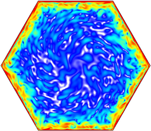
  $\epsilon$, the arms of the geostrophic shear impinge on the boundary layers, triggering ripples as the boundary-confined wave negotiates its way past the geostrophic shear. Figure 6(a) shows snapshots of the enstrophy density on the surface and in the equatorial and meridional planes for $ {\textit {E}}=10^{-5}$ for three values of $\epsilon$ above critical (the critical value has been bracketed to between $0.030$ and $0.031$). The supplementary movie 3 animates these over ten libration periods. For the smallest $\epsilon =0.031$ case, the surface animation shows the boundary-confined wave propagating essentially in the same fashion as it does for lower $\epsilon$; however, there are faint ripples evident near the equatorial vertices (these are the points on the cube furthest from the rotation axis). The animations in the equatorial and meridional planes are very similar to those at $\epsilon =0.030$ (see supplementary movie 2), except that in the boundary layers viewed in the equatorial plane, at approximately the distance of the first local minimum in the wall-normal enstrophy profile (the greenish contours in the animations), there is clear evidence of ripples sloshing back-and-forth with the libration of the cube. These ripples are more intense either side of where the arms of the geostrophic shear impinge on the boundary layers. The power spectral density (PSD) of the time series of a component of velocity at a point near the edge of the boundary layer has a main peak at the libration frequency $2\omega =2/\sqrt {3}\approx 1.155$ and a weaker peak at frequency $f_{NS}\approx 0.606$ that is introduced at a symmetry-breaking Neimark–Sacker bifurcation. The Neimark–Sacker bifurcation is a typical bifurcation from a limit cycle solution to a quasi-periodic (2-torus) solution as a control parameter is varied (Kuznetsov Reference Kuznetsov2004, Chapter 4). It is often encountered in parametrically forced fluid flows, for example the precessionally forced cylinder flow where it is associated with the triadic resonant instability (Marques & Lopez Reference Marques and Lopez2015). The main peaks in the PSD have side-bands corresponding to the beat frequency $f_{beat}=2f_{NS}-2\omega \approx 0.057$, which is also present as a peak in the PSD. Signatures of these frequencies are evident in the meridional plane, where beams at angles corresponding to $\arccos$ of $f_{NS}$ and $f_{NS}\pm f_{beat}$ are seen to emerge from the equatorial region, and beams at angles corresponding to $\arccos$ of $f_{beat}$ emerge from the poles. As $\epsilon$ is increased, the relative power in the $f_{beat}$ and $f_{NS}$ peaks increases and their linear combinations with $2\omega$ and its harmonics results in a broad-band PSD. The result is strong nonlinear interactions between the various corresponding beams leading to a type of wave turbulence throughout the entire cube. The boundary-confined wave is still very discernable in the surface plots, but the ripples now extend over the whole surface of the cube, as well as deep into the interior.
Snapshots at half-phase of the enstrophy density on the surface and in the equatorial and meridional planes at  $\epsilon$ and $ {\textit {E}}$ as indicated. The time-averaged symmetry measure $\bar {S}$ is indicated for each case. Supplementary movies 3 and 4 animate these over 10 libration periods. (a) $E = 10^{-5}$, (b) $E = 10^{-6}$.

The instability at  $ {\textit {E}}=10^{-6}$ is qualitatively similar, as evidenced by the plots in figure 6(b) and the corresponding animations in supplementary movie 4, but occurs at a much smaller Rossby number, $\epsilon$, between approximately 0.0028 and 0.0032. The beams due to $f_{beat}$ and $f_{NS}$ and their linear combinations with $2\omega$ are much clearer at the smaller $ {\textit {E}}$ and $\epsilon$. However, slightly increasing $\epsilon$ to 0.006 leads to wave turbulence so strong that we are unable to resolve it with $250^3$ spectral resolution and 800 time steps per libration period.
5. Conclusions
A cube librating around an axis passing through opposite vertices results in a configuration where all walls have critical slope for a libration frequency that is  $2/\sqrt {3}$ times the background rotation frequency. For rapid rotations ( $ {\textit {E}}\ll 1$) subjected to small libration amplitudes ( $\epsilon \ll {\textit {E}}^{1/2}$), the resulting inertial wave beams emanating from edges and vertices remain confined to the faces of the cube, with the fluid in the bulk being essentially static relative to the librating cube. The response flow reduces to a boundary-confined wave travelling on the surface of the cube. The thickness of the time average of this oscillatory boundary-layer flow scales with $ {\textit {E}}^{1/3}$, but the thickness over which the oscillation amplitudes are non-zero is much thinner, scaling with $ {\textit {E}}^{1/2}$. While these boundary-confined waves also are present at non-critical slope regimes, as observed in Wu et al. (Reference Wu, Welfert and Lopez2020), criticality helps reinforce and isolate them from other flow phenomena, such as inertial wave beams throughout the cube, thus facilitating the study of their dynamics with increasing forcing amplitude $\epsilon$. Nonlinear effects induce a mean flow that becomes non-negligible as $\epsilon$ approaches ${O}( {\textit {E}}^{1/2})$. The enstrophy of this quasi-geostrophic mean flow exhibits a six-armed pattern around the axis of rotation, which extends farther away from the axis with increasing $\epsilon$. This structure eventually interacts with the boundary-confined wave in the boundary layers, causing ripples travelling at a subharmonic frequency nearly half that of the forcing. This is an example of a wave–mean flow interaction (Bühler Reference Bühler2009). Inertial waves emanating from the vertices at angles associated with this frequency as well as multiples of the beat frequency create a network of beams in the bulk that quickly leads to complicated wave–wave interactions via nonlinearities upon further increase of $\epsilon$, while superharmonics of the forcing frequency are outside the inertial range and thus damped by viscous effects. This road to wave turbulence can be expected to occur whenever at least a portion of the container's boundary is critical, or even near critical. How the boundary-confined waves and the geostrophic flow then interact nonlinearly with the inertial wave beams in the interior of the container and the ensuing instabilities remain to be explored for critical Rossby numbers at very small Ekman numbers.
Supplementary movies
Supplementary movies are available at https://doi.org/10.1017/jfm.2022.934.
Funding
Simulations were performed on Purdue and ASU Research Computing facilities, with technical support from J. Yalim. J.S. and K.W. were partially supported by NSF DMS-2012585 and AFOSR FA9550-20-1-0309.
Declaration of interests
The authors report no conflict of interest.


 Open access