





1. Introduction
For more than four decades, researchers have observed the presence of thin layers of phytoplankton, characterised by dense concentrations of phytoplankton confined within narrow horizontal bands. These layers are accumulations of plankton in a narrow depth layer but extending over kilometres (Dekshenieks et al. Reference Dekshenieks, Donaghay, Sullivan, Rines, Osborn and Twardowski2001; Moline et al. Reference Moline, Benoit-Bird, Robbins, Schroth-Miller, Waluk and Zelenke2010), and the phytoplankton concentration can potentially be orders of magnitude higher than the background level (Ryan et al. Reference Ryan, McManus, Paduan and Chavez2008; Sullivan, Donaghay & Rines Reference Sullivan, Donaghay and Rines2010), forming important ecological activity hotspots. Due to their ecological significance, several fluid mechanic mechanisms have been proposed for the thin-layer formation, including straining (Franks Reference Franks1995; Osborn Reference Osborn1998), buoyancy (Alldredge et al. Reference Alldredge, Cowles, MacIntyre S, Rines, Donaghay, Greenlaw, Holliday, Dekshenieks, Sullivan and Zaneveld2002), intrusion (Armi Reference Armi1978; Phillips, Shyu & Salmun Reference Phillips, Shyu and Salmun1986; Kasai et al. Reference Kasai, Kurikawa, Ueno, Robert and Yamashita2010) and gyrotactic trapping (Durham, Kessler & Stocker Reference Durham, Kessler and Stocker2009). Those proposed mechanisms have been discussed in the review by Durham & Stocker (Reference Durham and Stocker2012).
The gyrotactic trapping mechanism is one of the most promising mechanisms for explaining motile, bottom-heavy phytoplankton accumulations, and it is consistent with field observations that the thin layer is frequently found at the depths where vertical shear, variation of horizontal velocity as a function of vertical distance, is enhanced (Dekshenieks et al. Reference Dekshenieks, Donaghay, Sullivan, Rines, Osborn and Twardowski2001; Seuront & Strutton Reference Seuront and Strutton2003; Ryan et al. Reference Ryan, McManus, Paduan and Chavez2008; Sullivan et al. Reference Sullivan, Donaghay and Rines2010). The balance of two types of torques leads to gyrotactic trapping. One is hydrodynamic torque, also called viscous torque. The hydrodynamic torque was originally derived in the seminal work by Jeffery (Reference Jeffery1922), where particles respond to local vorticity and rate of strain (applicable only to non-spherical particles). At the microswimmer length scale, the microswimmers experience a sea of gradients, and they experience linear hydrodynamic shear locally (Stocker Reference Stocker2012) because the body size of the microswimmers is much smaller than Kolmogorov length scales (Wheeler et al. Reference Wheeler, Secchi, Rusconi and Stocker2019). Gravitational torques arise from the fact that a microswimmer’s centre of mass is different from its geometric centre. Most gyrotactic phytoplankton are bottom heavy, i.e. the centre of mass is located lower than the geometric centre. Bottom-heavy phytoplankton generates a stabilising gravitational torque on the cell that acts to keep its swimming direction oriented opposite to gravity.
Much previous research has shown that the microswimmer/particle intrinsic mobility, hydrodynamic torque from local shear and gyrotaxis can independently or jointly generate preferential distribution in a wide range of flows. Kessler (Reference Kessler1985) set up the torque balance of a spherical motile cell and theoretically and experimentally demonstrated the gyrotactic focusing of the motile cells in Poiseuille flow. In addition, Durham, Climent & Stocker (Reference Durham, Climent and Stocker2011) demonstrate that the gyrotactic motility within a steady vorticial flow can cause a tightly clustered aggregation of microorganisms. A similar effect has also been observed by Khurana, Blawzdziewicz & Ouellette (Reference Khurana, Blawzdziewicz and Ouellette2011) and Yazdi & Ardekani (Reference Yazdi and Ardekani2012) with only motility effects. It has been found that the hydrodynamic shear (Rusconi, Guasto & Stocker Reference Rusconi, Guasto and Stocker2014) and flow velocity (Borgnino et al. Reference Borgnino, Gustavsson, De Lillo, Boffetta, Cencini and Mehlig2019) can have non-trivial impacts on the orientation and spatial heterogeneity of swimmers resulting from their shapes and intrinsic mobility, in which the fluid shear can trap swimmers (Rusconi et al. Reference Rusconi, Guasto and Stocker2014) and rod-like swimmers preferentially align with the flow velocity (Borgnino et al. Reference Borgnino, Gustavsson, De Lillo, Boffetta, Cencini and Mehlig2019). Turbulence can also lead to the heterogeneous distribution of swimmers and particles (Squires & Eaton Reference Squires and Eaton1991; Monchaux, Bourgoin & Cartellier Reference Monchaux, Bourgoin and Cartellier2011; Ray & Collins Reference Ray and Collins2011; Durham et al. Reference Durham, Climent, Barry, De Lillo, Boffetta, Cencini and Stocker2013; Obligado et al. Reference Obligado, Teitelbaum, Cartellier, Mininni and Bourgoin2014; Pujara, Koehl & Variano Reference Pujara, Koehl and Variano2018; Falkinhoff et al. Reference Falkinhoff, Obligado, Bourgoin and Mininni2020; Qiu, Marchioli & Zhao Reference Qiu, Marchioli and Zhao2022). In isotropic turbulence, ellipsoidal swimmers preferentially sample regions of lower fluid vorticity and accumulate in those regions (Pujara et al. Reference Pujara, Koehl and Variano2018). However, clustering and patchiness are much weaker in isotropic turbulence than in simple cellular or vortical flows (Torney & Neufeld Reference Torney and Neufeld2007; Khurana et al. Reference Khurana, Blawzdziewicz and Ouellette2011) due to the complex topology (Zhan et al. Reference Zhan, Sardina, Lushi and Brandt2014). (Lovecchio et al. Reference Lovecchio, Climent, Stocker and Durham2019) demonstrated that chain formation in motile phytoplankton significantly enhances their ability to migrate vertically in turbulent waters, especially under weak to moderate turbulence. (Gustavsson et al. Reference Gustavsson, Berglund, Jonsson and Mehlig2016) and (Borgnino et al. Reference Borgnino, Boffetta, De Lillo and Cencini2018) complemented the analysis presented in (Lovecchio et al. Reference Lovecchio, Climent, Stocker and Durham2019), particularly discussed the effect of shape in sampling up-welling/down-welling regions of turbulence and the role of swimming speed. Si & Fang have revealed the preferential accumulation of non-spherical motile swimmers’ accumulation near Lagrangian coherent structures (Si & Fang Reference Si and Fang2021) and three regimes of preferential transport of such swimmers in strongly heterogeneous two-dimensional weakly turbulent flow with heterogeneous Reynolds number along one direction (Si & Fang Reference Si and Fang2022).
Hydrodynamic torque, gravitational torque as well as microswimmer’s intrinsic motility can also combine to generate a clustering of thin layers at the surface of water bodies. In natural water bodies, the shear rate typically decreases with increasing depth. (Durham et al. Reference Durham, Kessler and Stocker2009) showed that thin layers form at a depth where the shear rate exceeds a critical value $S_{C}$
. Above the critical shear, hydrodynamic torque dominates, causing continuous cell rotation and resulting in a sinking motion due to settling velocity. Below the critical shear, gyrotactic forces stabilise the cell, allowing it to move upward while encountering higher shear. As a result, the swimmer tends to become trapped at the critical shear layer. At critical shear, the cell’s upward speed vanishes, leading to an accumulation of cells. The critical shear is derived based on torque balance and is equal to the inverse of the gyrotactic time scale (
$S_{C}$
. Above the critical shear, hydrodynamic torque dominates, causing continuous cell rotation and resulting in a sinking motion due to settling velocity. Below the critical shear, gyrotactic forces stabilise the cell, allowing it to move upward while encountering higher shear. As a result, the swimmer tends to become trapped at the critical shear layer. At critical shear, the cell’s upward speed vanishes, leading to an accumulation of cells. The critical shear is derived based on torque balance and is equal to the inverse of the gyrotactic time scale ( $\tau$
), which
$\tau$
), which $\tau$
is known for a variety of species and is generally within 1–100 s (Kessler Reference Kessler1985; Hill & Häder Reference Hill and Häder1997; Drescher et al. Reference Drescher, Leptos, Tuval, Ishikawa, Pedley and Goldstein2009; Durham et al. Reference Durham, Kessler and Stocker2009). (Santamaria et al. Reference Santamaria, De Lillo, Cencini and Boffetta2014) investigated spherical gyrotactic trapping in Kolmogorov flows and discussed the effects of turbulence fluctuation on thin-layer formation. Bearon & Durham (Reference Bearon and Durham2023) explored elongated gyrotactic trapping in Kolmogorov flow. (Berman et al. Reference Berman, Ferguson, Bizzak, Solomon and Mitchell2022) assessed the effect of elongation in steady Kolmogorov, while (Borgnino et al. Reference Borgnino, Boffetta, Cencini, De Lillo and Gustavsson2022) investigated that effect both in steady and unsteady Kolmogorov flows.
$\tau$
is known for a variety of species and is generally within 1–100 s (Kessler Reference Kessler1985; Hill & Häder Reference Hill and Häder1997; Drescher et al. Reference Drescher, Leptos, Tuval, Ishikawa, Pedley and Goldstein2009; Durham et al. Reference Durham, Kessler and Stocker2009). (Santamaria et al. Reference Santamaria, De Lillo, Cencini and Boffetta2014) investigated spherical gyrotactic trapping in Kolmogorov flows and discussed the effects of turbulence fluctuation on thin-layer formation. Bearon & Durham (Reference Bearon and Durham2023) explored elongated gyrotactic trapping in Kolmogorov flow. (Berman et al. Reference Berman, Ferguson, Bizzak, Solomon and Mitchell2022) assessed the effect of elongation in steady Kolmogorov, while (Borgnino et al. Reference Borgnino, Boffetta, Cencini, De Lillo and Gustavsson2022) investigated that effect both in steady and unsteady Kolmogorov flows.
Despite valuable insights from gyrotactic swimmers in Kolmogorov flow, significant opportunities remain in understanding the gyrotactic trapping mechanisms driving thin-layer generation in the depth-independent shear environments typical of oceans and lakes. A few key questions remain unanswered. First, how does the swimmer shape affect the formation of the thin layer? Second, how quickly does this thin layer emerge, i.e. what is the time scale of thin-layer accumulation? Third, how will the time-dependent flow modulate the thin layer? In this paper, we aim to address these knowledge gaps.
We start in § 2 by introducing the equations for torque balance, reviewing the equations for particle rotational motion and their simplification, and verifying our model. In § 3, we study the impact of a swimmer’s non-spherical shape on thin-layer formation, deriving the thin-layer accumulation time scale, and reveal three distinct mechanisms for thin-layer accumulation when the background flow is time-dependent. We conclude our work in § 4.
2. Methods
2.1. Torque balance and agent-based model
We simulate particles as spheroids of which the sizes are described by $d_s$
, the diameter of the equivalent sphere with the same volume as the spheroid. The shapes are described by
$d_s$
, the diameter of the equivalent sphere with the same volume as the spheroid. The shapes are described by $\lambda$
, the aspect ratio given by
$\lambda$
, the aspect ratio given by $a/b$
, where
$a/b$
, where $a$
is the length along the particle’s axis of symmetry and
$a$
is the length along the particle’s axis of symmetry and $b$
is the length of one of the orthogonal axes (figure 1). Here,
$b$
is the length of one of the orthogonal axes (figure 1). Here, $L$
is the distance between the centroid and the centre of mass, while
$L$
is the distance between the centroid and the centre of mass, while $T_g=mgL \sin \phi$
is the gravitational torque due to the bottom-heavy characteristic, where m is the mass of the microswimmer, g is the acceleration due to gravity,
$T_g=mgL \sin \phi$
is the gravitational torque due to the bottom-heavy characteristic, where m is the mass of the microswimmer, g is the acceleration due to gravity, $\phi$
is the angle from the
$\phi$
is the angle from the $z$
-axis to the swimming direction
$z$
-axis to the swimming direction $\boldsymbol{p}$
, i.e. the polar angle. Conceptually, the polar angle
$\boldsymbol{p}$
, i.e. the polar angle. Conceptually, the polar angle $\phi$
spans the range [–
$\phi$
spans the range [– $\pi$
,
$\pi$
, $\pi$
]. However, as the primary focus of this paper is on the formation of thin layers, lateral displacement in the
$\pi$
]. However, as the primary focus of this paper is on the formation of thin layers, lateral displacement in the $x$
-direction is not our main interest. Therefore, we restrict
$x$
-direction is not our main interest. Therefore, we restrict $\phi$
to [0,
$\phi$
to [0, $\pi$
], treating negative values of
$\pi$
], treating negative values of $\phi$
as their positive counterparts by mirroring them across the
$\phi$
as their positive counterparts by mirroring them across the $z$
-axis. In this paper, we considered prolate (
$z$
-axis. In this paper, we considered prolate ( $\lambda \gt 1$
) spheroids since most gyrotactic microswimmers are prolate.
$\lambda \gt 1$
) spheroids since most gyrotactic microswimmers are prolate.
Sketch of ellipsoidal microswimmer. Only prolate spheroidal particles are considered, as no gyrotactic microswimmers are oblate. Here, $a$
represents the length of the long semi-axis while
$a$
represents the length of the long semi-axis while $b=c$
are the lengths of the short semi-axes for axisymmetric ellipsoids. The hydrodynamic shear lies in the
$b=c$
are the lengths of the short semi-axes for axisymmetric ellipsoids. The hydrodynamic shear lies in the $x$
–
$x$
– $z$
plane (the
$z$
plane (the $y$
-axis points into the page), and only
$y$
-axis points into the page), and only $\partial u_x/\partial z$
is non-zero. The angle between vertical direction (
$\partial u_x/\partial z$
is non-zero. The angle between vertical direction ( $z$
-axis) and swimming orientation (
$z$
-axis) and swimming orientation ( $\boldsymbol{p}$
) is the polar angle
$\boldsymbol{p}$
) is the polar angle $\phi$
. Here,
$\phi$
. Here, $L$
is the distance from the centroid to the centre of gravity. In the schematic, the flagella are shown only to indicate the direction of swimming.
$L$
is the distance from the centroid to the centre of gravity. In the schematic, the flagella are shown only to indicate the direction of swimming.

Starting from the equation of hydrodynamic torque $\boldsymbol{T}$
for ellipsoids in general shear flow shown in Jeffery’s seminal paper (Jeffery Reference Jeffery1922)
$\boldsymbol{T}$
for ellipsoids in general shear flow shown in Jeffery’s seminal paper (Jeffery Reference Jeffery1922)
 \begin{align} \boldsymbol{T} &= \begin{pmatrix} T_{x} \\[4pt] T_{y} \\[4pt] T_{z} \end{pmatrix} = \frac {16\pi \mu a^3}{3} \begin{pmatrix} \dfrac {b^2+c^2}{b^2\beta _0+c^2\gamma _0} \left (\dfrac {b^2-c^2}{b^2+c^2} S_{zy} + (\Omega _{zy}-\omega _x) \right ) \\[12pt] \dfrac {c^2+a^2}{c^2\gamma _0+a^2\alpha _0} \left ( \dfrac {c^2-a^2}{c^2+a^2} S_{xz} + (\Omega _{xz}-\omega _y) \right ) \\[12pt]\dfrac {a^2+b^2}{a^2\alpha _0+b^2\beta _0} \left ( \dfrac {a^2-b^2}{a^2+b^2} S_{yx} + (\Omega _{yx}-\omega _z) \right ) \end{pmatrix}\kern-2.5pt, \end{align}
where $S_{ij} = ({1}/{2})\;(\partial _ju_i +\partial _iu_j )$
,
$S_{ij} = ({1}/{2})\;(\partial _ju_i +\partial _iu_j )$
, $\Omega _{ij} = ({1}/{2})\;(\boldsymbol{\nabla }\times \boldsymbol{u})$
,
$\Omega _{ij} = ({1}/{2})\;(\boldsymbol{\nabla }\times \boldsymbol{u})$
, $\boldsymbol {u}$
is the velocity of the background flow,
$\boldsymbol {u}$
is the velocity of the background flow, $U_x$
is the horizontal component of the background velocity field and
$U_x$
is the horizontal component of the background velocity field and $\omega _i$
is particle’s angular velocity. The shape parameters
$\omega _i$
is particle’s angular velocity. The shape parameters $\alpha _0$
,
$\alpha _0$
, $\beta _0$
and
$\beta _0$
and $\gamma _0$
are given by,
$\gamma _0$
are given by,
 \begin{align} \alpha _0 = \int _0^\infty \frac {\mathrm{d}h}{(a^2+h)\varDelta },\ \ \beta _0 = \int _0^\infty \frac {\mathrm{d}h}{(b^2+h)\varDelta },\ \ \gamma _0 = \int _0^\infty \frac {\mathrm{d}h}{(c^2+h)\varDelta }, \end{align}
where $\varDelta = [(a^2+h)(b^2+h)(c^2+h)]^{1/2}$
, and
$\varDelta = [(a^2+h)(b^2+h)(c^2+h)]^{1/2}$
, and $a, b$
and
$a, b$
and $c$
are the semi-axes lengths along three axes for triaxial ellipsoids. The formula for shape factor integrals are provided in table 1.
$c$
are the semi-axes lengths along three axes for triaxial ellipsoids. The formula for shape factor integrals are provided in table 1.
Solution of shape factor integrals for ellipsoids with $b=c$
and
$b=c$
and $a = b\lambda$
.
$a = b\lambda$
.

Assuming the shear flow is generated by the vertical gradients of velocity in the $x$
–
$x$
– $z$
plane, the sum of hydrodynamic and gravitational torques on an ellipsoid can be written as
$z$
plane, the sum of hydrodynamic and gravitational torques on an ellipsoid can be written as
 \begin{align} T_y = \frac {16\pi \mu a^3}{3} \left [ \frac {b^2+a^2}{b^2\beta _0+a^2\alpha _0} \left (\frac {b^2-a^2}{b^2+a^2} \frac {\partial u_x}{\partial z} + (\Omega _y-\omega _y) \right ) \right ] -mgL\sin {\phi }, \end{align}
The first term on the right-hand side involves the contribution of hydrodynamic torque. Both rate of strain and vorticity contribute to the hydrodynamic torque for non-spherical particles, while only vorticity contributes to the hydrodynamic torque when a swimmer is spherical. The second term on the right-hand side is gravitational torque. By setting $T_y=0$
, and
$T_y=0$
, and $\omega _y=0$
, the static torque balance yields a constant polar angle
$\omega _y=0$
, the static torque balance yields a constant polar angle $\phi$
for time-independent shear rate,
$\phi$
for time-independent shear rate,
 \begin{align} \sin {\phi } = \frac {16\pi \mu a^3}{3mgL}\left ( \frac {b^2}{b^2\beta _0+a^2\alpha _0} \right )\frac {\partial u_x}{\partial z} = \tau \frac {\partial u_x}{\partial z}, \end{align}
where $\tau$
is the gyrotactic reorientation time scale, referring to the characteristic time it takes for microswimmers to reorient themselves due to gravitational torque.
$\tau$
is the gyrotactic reorientation time scale, referring to the characteristic time it takes for microswimmers to reorient themselves due to gravitational torque.
Substituting the volume calculation formula of spheroids, $V = 4/3\pi a^2b$
, into (2.4), a simplified expression of
$V = 4/3\pi a^2b$
, into (2.4), a simplified expression of $\tau$
can be obtained
$\tau$
can be obtained
 \begin{align} \tau &= \frac {4\nu }{BgL(\beta _0/\lambda ^2+\alpha _0)}, \end{align}
where $B$
is the buoyancy, which is the density ratio of particle to fluid. With the gyrotactic reorientation time scale (
$B$
is the buoyancy, which is the density ratio of particle to fluid. With the gyrotactic reorientation time scale ( $\tau$
), the equation of torque can be simplified as
$\tau$
), the equation of torque can be simplified as
 \begin{align} T_y&= mgL\tau \left [ \frac {\partial u_x}{\partial z} - (1+\lambda ^2)\omega _y - \frac {\sin {\phi }}{\tau } \right ]\kern-2.5pt. \end{align}
Then, the angular acceleration can be derived as
 \begin{align} \dot {\omega }_y = \frac {T_y}{I_y} &= -\frac {5gL\tau }{b^2}\omega _y + \frac {5gL\tau }{a^2+b^2}\left [ \frac {\partial u_x}{\partial z} - \frac {\sin {\phi }}{\tau } \right ]\kern-2.5pt, \end{align}
where $I_y$
is the moment of inertia of the ellipsoidal swimmers. The angular velocity can be solved as
$I_y$
is the moment of inertia of the ellipsoidal swimmers. The angular velocity can be solved as
 \begin{align} \omega _y &= -\frac {1}{\lambda ^2+1} \left ( \frac {\partial u_x}{\partial z}\bigg |_{t=0} - \frac {\sin {\phi _0}}{\tau } \right )\mathrm{e}^{-\frac {5gL\tau }{b^2}t} + \frac {1}{1 + \lambda ^2}\left ( \frac {\partial u_x}{\partial z} - \frac {\sin {\phi }}{\tau } \right)\kern-2.5pt, \end{align}
where $\phi _0$
is the initial polar angle. We arrive at the question of the motion of angular velocity of an ellipsoid particle experiencing both viscous and gravitational torques. Since we assume that flow has no velocity out of the
$\phi _0$
is the initial polar angle. We arrive at the question of the motion of angular velocity of an ellipsoid particle experiencing both viscous and gravitational torques. Since we assume that flow has no velocity out of the $x$
–
$x$
– $z$
plane, the angular velocity is a scalar. Moreover, the angular velocity consists of an exponentially decaying time-varying part and a steady part.
$z$
plane, the angular velocity is a scalar. Moreover, the angular velocity consists of an exponentially decaying time-varying part and a steady part.
To determine how quickly the first term decays, we quantify the magnitude of its decaying time scale
 \begin{align} t_{\textit{decay}} = \frac {b^2}{5gL\tau } = \frac {Bb^2(\beta _0 + \lambda ^2\alpha _0)}{20\nu \lambda ^2}. \end{align}
The decay time scale is a function of both the swimmer’s size and shape. Figure 2 shows $t_{\textit{decay}}$
is smaller than
$t_{\textit{decay}}$
is smaller than $10^{-2}$
s when
$10^{-2}$
s when $d_s$
is smaller than
$d_s$
is smaller than $10^{-3}$
m for
$10^{-3}$
m for $\lambda$
between 1 and 5, meaning the system is highly damped and inertia can be ignored even for relatively large swimmers such as Euglena gracilis, Ceratium and species belong to Copepod. Most gyrotactic microswimmers are smaller than
$\lambda$
between 1 and 5, meaning the system is highly damped and inertia can be ignored even for relatively large swimmers such as Euglena gracilis, Ceratium and species belong to Copepod. Most gyrotactic microswimmers are smaller than $10^{-3}$
m and have an aspect ratio between 1 and 5. Based on that, we proposed an agent-based model for gyrotactic ellipsoidal swimmers
$10^{-3}$
m and have an aspect ratio between 1 and 5. Based on that, we proposed an agent-based model for gyrotactic ellipsoidal swimmers
 \begin{align} \omega _y &= \frac {1}{1+\lambda ^2} \left ( \frac {\partial u_x}{\partial z} - \frac {\sin {\phi }}{\tau }\right)\kern-2.5pt,\\[-10pt]\nonumber\end{align}
 \begin{align} \boldsymbol{v}& = \boldsymbol{u} + v_p\boldsymbol{p} + \boldsymbol{v}_{\textit{settle}},\\[-10pt]\nonumber\end{align}
 \begin{align} \phi &= \omega _y\Delta t +\Delta \phi , \end{align}
where $\boldsymbol{u}$
is the velocity of background flow while
$\boldsymbol{u}$
is the velocity of background flow while $\boldsymbol{p}$
indicates the swimming direction.
$\boldsymbol{p}$
indicates the swimming direction. $\boldsymbol{v}_{\textit{settle}}$
is the settling velocity, which can be written as
$\boldsymbol{v}_{\textit{settle}}$
is the settling velocity, which can be written as
 \begin{align} \boldsymbol{v}_{\textit{settle}} &= -v_1\boldsymbol{e}_z - (v_3-v_1)(\boldsymbol{e}_z\boldsymbol{\cdot} \boldsymbol{p})\boldsymbol{p}, \end{align}
where $v_1$
and
$v_1$
and $v_3$
are the Stokesian terminal velocities of a spheroid in a quiescent fluid with its symmetry axis orientated orthogonal to and parallel to the gravity direction. To describe randomness existing in the swimming direction of a group of swimmers, we add noise at each time step, which is modelled as
$v_3$
are the Stokesian terminal velocities of a spheroid in a quiescent fluid with its symmetry axis orientated orthogonal to and parallel to the gravity direction. To describe randomness existing in the swimming direction of a group of swimmers, we add noise at each time step, which is modelled as $\Delta \phi = \pm (2D_R\Delta t)^{1/2}$
with rotational diffusivity
$\Delta \phi = \pm (2D_R\Delta t)^{1/2}$
with rotational diffusivity $D_R = 0.01\,\rm s^{-1}$
(Durham et al. Reference Durham, Kessler and Stocker2009).
$D_R = 0.01\,\rm s^{-1}$
(Durham et al. Reference Durham, Kessler and Stocker2009).
Colour map of the decaying time scale $t_{\textit{decay}}$
with equivalent diameter
$t_{\textit{decay}}$
with equivalent diameter $d_s$
and aspect ratio
$d_s$
and aspect ratio $\lambda$
. The colour bar is presented on a logarithmic scale.
$\lambda$
. The colour bar is presented on a logarithmic scale.

2.2. Model verification
To verify our agent-based model of spheroidal microswimmers, we utilise the parameters of a typical gyrotactic microswimmer, Chlamydomonas nivalis, in our simulation, with $v_p=80\ \mathrm{\unicode{x03BC} m\,s^{-1}}$
,
$v_p=80\ \mathrm{\unicode{x03BC} m\,s^{-1}}$
, $d_s = 10\ \mathrm{\unicode{x03BC} m}$
,
$d_s = 10\ \mathrm{\unicode{x03BC} m}$
, $B=1.05$
and
$B=1.05$
and $L=0.06\ \mathrm{\unicode{x03BC} m}$
. When setting
$L=0.06\ \mathrm{\unicode{x03BC} m}$
. When setting $\lambda$
= 1.001, we recover the experimental conditions of (Durham et al. Reference Durham, Kessler and Stocker2009). The background flow is assumed to be a linear shear flow with kinematic viscosity
$\lambda$
= 1.001, we recover the experimental conditions of (Durham et al. Reference Durham, Kessler and Stocker2009). The background flow is assumed to be a linear shear flow with kinematic viscosity $\nu = 1\times 10^{-6}\, \mathrm{m^2\,s^{-1}}$
. The shear rate can be expressed as
$\nu = 1\times 10^{-6}\, \mathrm{m^2\,s^{-1}}$
. The shear rate can be expressed as $\partial u/\partial z=3z-0.3$
, which varies linearly from –0.3 to 0.6
$\partial u/\partial z=3z-0.3$
, which varies linearly from –0.3 to 0.6 $\mathrm{s}^{-1}$
when
$\mathrm{s}^{-1}$
when $z$
changes from 0 to 0.3 m (figure 3). Initially, 500 spheroidal active particles are released at
$z$
changes from 0 to 0.3 m (figure 3). Initially, 500 spheroidal active particles are released at $x$
= 0 m and
$x$
= 0 m and $z$
= 0.1 m with uniformly distributed random orientations. The time step is set to 0.01 s.
$z$
= 0.1 m with uniformly distributed random orientations. The time step is set to 0.01 s.
Flow conditions: (a) velocity profile and (b) shear profile of the background flow.

Time evolution of the heights of a group of microswimmers with (a) $\lambda$
= 1.001, (b)
$\lambda$
= 1.001, (b) $\lambda$
= 2 and (c)
$\lambda$
= 2 and (c) $\lambda$
= 3. The black dashed line represents the theoretical prediction of the depth of critical shear (
$\lambda$
= 3. The black dashed line represents the theoretical prediction of the depth of critical shear ( $1/\tau$
) according to (2.5), while the blue dashed line shows the average ensemble depth of the thin layer from the simulation.
$1/\tau$
) according to (2.5), while the blue dashed line shows the average ensemble depth of the thin layer from the simulation.

Figure 4 shows time variations in the depth of a group of gyrotactic microswimmers with different body shapes, and the dashed lines are the predicted accumulation depths. We observe that microswimmers accumulate near the predicted critical shear depths. In the beginning, the swimmers are located in a region with relatively low shear ( $z = 0.1$
m) with random orientation. The gravitational torque dominates the rotational motion, directing the microswimmers to go upward. However, when microswimmers go above the theoretically predicted depth, the hydrodynamic torque dominates and drives microswimmers to rotate continuously. When the swimmer rotates continuously, its intrinsic mobility lacks directional bias in the vertical direction, and the gravitational settling moves the microswimmers downward gradually. Finally, those swimmers will accumulate at a specific height, where local shear is equal to critical shear, and form a thin layer in the background flow. Due to the rotational diffusivity in the simulation, the microswimmers’ orientations will be perturbed, and the aforementioned process will continue. When
$z = 0.1$
m) with random orientation. The gravitational torque dominates the rotational motion, directing the microswimmers to go upward. However, when microswimmers go above the theoretically predicted depth, the hydrodynamic torque dominates and drives microswimmers to rotate continuously. When the swimmer rotates continuously, its intrinsic mobility lacks directional bias in the vertical direction, and the gravitational settling moves the microswimmers downward gradually. Finally, those swimmers will accumulate at a specific height, where local shear is equal to critical shear, and form a thin layer in the background flow. Due to the rotational diffusivity in the simulation, the microswimmers’ orientations will be perturbed, and the aforementioned process will continue. When $\lambda$
= 1.001, we observe a thin-layer accumulation where the local shear is approximately 0.2
$\lambda$
= 1.001, we observe a thin-layer accumulation where the local shear is approximately 0.2 $\mathrm{s}^{-1}$
, which is consistent with the (Durham et al. Reference Durham, Kessler and Stocker2009) experiments with nearly spherical microswimmers (Chlamydomonas nivalis). The reproduction of the experimental observation shows that our simulation is reliable.
$\mathrm{s}^{-1}$
, which is consistent with the (Durham et al. Reference Durham, Kessler and Stocker2009) experiments with nearly spherical microswimmers (Chlamydomonas nivalis). The reproduction of the experimental observation shows that our simulation is reliable.
(a) The PDFs of the depths of microswimmers at steady states with a series of aspect ratios from 1.001 to 3. The vertical dashed lines indicate the theoretical predictions of the depth of critical shears ( $1/\tau$
). The inset shows the standard deviations of the PDFs as a function of
$1/\tau$
). The inset shows the standard deviations of the PDFs as a function of $\lambda$
, where the standard deviations characterise the thickness of the thin layer. (b) Comparison of critical shear between numerical results and theoretical prediction. The inset figure shows numerical accumulation depth and corresponding theoretical predictions.
$\lambda$
, where the standard deviations characterise the thickness of the thin layer. (b) Comparison of critical shear between numerical results and theoretical prediction. The inset figure shows numerical accumulation depth and corresponding theoretical predictions.

3. Results and discussion
3.1. Effects of shape
The seminal work of (Durham et al. Reference Durham, Kessler and Stocker2009) demonstrated that the critical shear $S_C$
, at which gyrotactic microswimmers accumulate, can be predicted as
$S_C$
, at which gyrotactic microswimmers accumulate, can be predicted as $1/\tau$
based on the torque balance equation. The critical shear,
$1/\tau$
based on the torque balance equation. The critical shear, $S_C$
=
$S_C$
= $1/\tau$
, arises from the torque balance between hydrodynamic and gravitational torques acting on a gyrotactic microswimmer. At steady state, (2.10) simplifies to
$1/\tau$
, arises from the torque balance between hydrodynamic and gravitational torques acting on a gyrotactic microswimmer. At steady state, (2.10) simplifies to $\partial u/\partial z = \sin {\phi }/\tau$
. Considering that the settling speed is much smaller than the swimming speed, the steady polar angle
$\partial u/\partial z = \sin {\phi }/\tau$
. Considering that the settling speed is much smaller than the swimming speed, the steady polar angle $\phi$
is close to
$\phi$
is close to $\pi /2$
, meaning
$\pi /2$
, meaning $\sin {\phi }$
is close to 1. Thus, the critical shear is approximately
$\sin {\phi }$
is close to 1. Thus, the critical shear is approximately $1/\tau$
. When we consider ellipsoid microswimmers of the same
$1/\tau$
. When we consider ellipsoid microswimmers of the same $d_s$
, the larger aspect ratios
$d_s$
, the larger aspect ratios $\lambda$
alter the gyrotactic time scale
$\lambda$
alter the gyrotactic time scale $\tau$
, leading to a smaller
$\tau$
, leading to a smaller $S_C$
(2.5). Additional observation can be done for figure 4, when simulations reach a steady state. Here, steady state refers to a statistically stationary condition where ensemble-averaged quantities, such as mean depth
$S_C$
(2.5). Additional observation can be done for figure 4, when simulations reach a steady state. Here, steady state refers to a statistically stationary condition where ensemble-averaged quantities, such as mean depth $z$
and polar angle
$z$
and polar angle $\phi$
, stabilise without consistent directional changes over a sufficiently long time window, even though individual trajectories may oscillate due to time-dependent shear or rotational diffusivity. As the aspect ratio of the microswimmer increases, the microswimmers are observed to accumulate at a smaller critical shear level.
$\phi$
, stabilise without consistent directional changes over a sufficiently long time window, even though individual trajectories may oscillate due to time-dependent shear or rotational diffusivity. As the aspect ratio of the microswimmer increases, the microswimmers are observed to accumulate at a smaller critical shear level.
In addition, we observe some nuanced behaviour of the accumulation depth in figure 5. The accumulation depth is typically slightly higher than the predicted critical shear depth. In figure 5(a), we see that the peaks of the probability density functions (PDFs) of the accumulation depths are higher than the critical shear depths. A similar effect is also seen in figure 5(b). The reason behind this is closely related to the mechanism of the thin-layer generation. Below the critical shear depth, the gravitational torque dominates, and microswimmers tend to move upward due to intrinsic mobility. Above critical shear hydrodynamic torque dominates, and microswimmers rotate continuously. As a result of this rotation, the intrinsic mobility contributes negligibly to the net vertical displacement, and microswimmers sink due to gravitational settling. The microswimmers’ settling velocities are much smaller than their intrinsic mobility, as shown in figure 6. Hence, the time for microswimmers to stay above the critical shear is longer than the time below in the predicted critical shear. Consequently, the thin layer appeared to be a little above the critical shear depth. This phenomenon was also observed in the experiments of (Durham et al. Reference Durham, Kessler and Stocker2009).
(a) Plot of $\sqrt {v_p^2-4(v_3-v_1)v_1}$
against the body lengths of four common types of gyrotactic microswimmers (Titelman Reference Titelman2001; Titelman & Kiørboe Reference Titelman and Kiørboe2003; Carlotti, Bonnet & Halsband-Lenk Reference Carlotti, Bonnet and Halsband-Lenk2007; Sohn et al. Reference Sohn, Seo, Choi, Lee, Kang and Kang2011). (b) The ratio of swimming speed and settling speed as a function of body length.
$\sqrt {v_p^2-4(v_3-v_1)v_1}$
against the body lengths of four common types of gyrotactic microswimmers (Titelman Reference Titelman2001; Titelman & Kiørboe Reference Titelman and Kiørboe2003; Carlotti, Bonnet & Halsband-Lenk Reference Carlotti, Bonnet and Halsband-Lenk2007; Sohn et al. Reference Sohn, Seo, Choi, Lee, Kang and Kang2011). (b) The ratio of swimming speed and settling speed as a function of body length.

In addition, the larger aspect ratios will also lead to thicker layers. This is evidenced by the more scattered trajectories while the aspect ratio $\lambda$
increases (figure 4). In figure 5(a), we observe that the PDF is more widespread as the aspect ratio increases. In the inset, we plot the PDFs’ standard deviation as the characterisation of the thin-layer thickness, and we observe a monotonic increase in layer thickness with an increase in the aspect ratio.
$\lambda$
increases (figure 4). In figure 5(a), we observe that the PDF is more widespread as the aspect ratio increases. In the inset, we plot the PDFs’ standard deviation as the characterisation of the thin-layer thickness, and we observe a monotonic increase in layer thickness with an increase in the aspect ratio.
The thicker layer for microswimmers with larger aspect ratios can be explained by carefully observing (2.10). Particles rotate slower with increasing $\lambda$
due to a larger
$\lambda$
due to a larger $\lambda ^2+1$
in the denominator of angular velocity. In addition, larger aspect ratio microswimmers tend to accumulate at the depth with smaller shear, leading to a further decrease in the rotation rate. During the thin-layer accumulation, the microswimmers usually continuously rotate once their position is higher than the critical shear such that the microswimmer’s intrinsic mobility is rotated in all possible directions in the
$\lambda ^2+1$
in the denominator of angular velocity. In addition, larger aspect ratio microswimmers tend to accumulate at the depth with smaller shear, leading to a further decrease in the rotation rate. During the thin-layer accumulation, the microswimmers usually continuously rotate once their position is higher than the critical shear such that the microswimmer’s intrinsic mobility is rotated in all possible directions in the $x$
–
$x$
– $z$
plane. Over one rotation period in the
$z$
plane. Over one rotation period in the $x$
–
$x$
– $z$
plane, the intrinsic mobility of the swimmer causes displacement in all directions, resulting in a net displacement in the
$z$
plane, the intrinsic mobility of the swimmer causes displacement in all directions, resulting in a net displacement in the $z$
-direction that is almost zero. The net-zero vertical displacement notwithstanding, the trajectories in
$z$
-direction that is almost zero. The net-zero vertical displacement notwithstanding, the trajectories in $t$
–
$t$
– $z$
space will be a sinuous line. The radius of curvature of the trajectory increases as the rotation rate decreases. When the microswimmer’s aspect ratio increases, the rotation becomes slower, and the radius of curvature increases, causing thicker thin-layer accumulation.
$z$
space will be a sinuous line. The radius of curvature of the trajectory increases as the rotation rate decreases. When the microswimmer’s aspect ratio increases, the rotation becomes slower, and the radius of curvature increases, causing thicker thin-layer accumulation.
3.2. The time scale of thin-layer accumulation
In addition to the gyrotactic time scale, there is also an important time scale: the time scale for microswimmers to accumulate at the thin layer ( $t_d$
), which is crucial for understanding how microswimmers accumulate in time-dependent flows where critical shear depth is changing. We rewrite (2.10) as (3.1) and focus on the
$t_d$
), which is crucial for understanding how microswimmers accumulate in time-dependent flows where critical shear depth is changing. We rewrite (2.10) as (3.1) and focus on the $z$
component of (2.12) to obtain (3.2). These two differential equations describe the variation of polar angle
$z$
component of (2.12) to obtain (3.2). These two differential equations describe the variation of polar angle $\phi$
and vertical position
$\phi$
and vertical position $z$
for microswimmers, while noise is neglected. Here, we perform a linear stability analysis on the following dynamic system:
$z$
for microswimmers, while noise is neglected. Here, we perform a linear stability analysis on the following dynamic system:
 \begin{align} \frac {\mathrm{d}\phi }{\mathrm{d}t} &= \frac {1}{1+\lambda ^2}\left ( \frac {\partial u_x}{\partial z} - \frac {p_x}{\tau }\right)\kern-2.5pt, \end{align}
 \begin{align} \frac {\mathrm{d}z}{\mathrm{d}t} &= v_pp_z -\left [ v_1+(v_3-v_1)p^2_z \right ]\kern-2.5pt, \end{align}
where $u_x$
is the projection of flow speed in the
$u_x$
is the projection of flow speed in the $x$
direction,
$x$
direction, $p_x$
is the projection of the swimming direction vector
$p_x$
is the projection of the swimming direction vector $\boldsymbol{p}$
onto the
$\boldsymbol{p}$
onto the $x$
-axis and
$x$
-axis and $p_z$
is the projection of
$p_z$
is the projection of $\boldsymbol{p}$
onto the
$\boldsymbol{p}$
onto the $z$
-axis. The fixed point is obtained as
$z$
-axis. The fixed point is obtained as
 \begin{align} \cos {\phi ^*} &= \frac {v_p-\sqrt {v^2_p-4(v_3-v_1)v_1}}{2(v_3-v_1)}, \end{align}
 \begin{align} S(z^*) &= \frac {\sqrt {1-\cos ^2\phi ^*}}{\tau }, \end{align}
 \begin{align} v_p\cos {\phi ^*} &= v_1+(v_3-v_1)\cos ^2{\phi ^*} = v_s, \end{align}
where $z^*$
and
$z^*$
and $\phi ^*$
are steady-state solutions to the dynamical system and
$\phi ^*$
are steady-state solutions to the dynamical system and $v_s$
is the vertical component of
$v_s$
is the vertical component of $\boldsymbol{v}_{\textit{settle}}$
. To ensure the existence of the fixed points, we compare the values of
$\boldsymbol{v}_{\textit{settle}}$
. To ensure the existence of the fixed points, we compare the values of $v_p^2$
and
$v_p^2$
and $4(v_3 - v_1)v_1$
for a series of common gyrotactic swimmer species in figure 6(a). Typically, a microswimmer’s intrinsic mobility is much larger than the settling velocity (Kamykowski, Reed & Kirkpatrick Reference Kamykowski, Reed and Kirkpatrick1992), ensuring that fixed points always exist for microswimmers. To analyse the stability of the equilibrium points, the Jacobian is derived as follows:
$4(v_3 - v_1)v_1$
for a series of common gyrotactic swimmer species in figure 6(a). Typically, a microswimmer’s intrinsic mobility is much larger than the settling velocity (Kamykowski, Reed & Kirkpatrick Reference Kamykowski, Reed and Kirkpatrick1992), ensuring that fixed points always exist for microswimmers. To analyse the stability of the equilibrium points, the Jacobian is derived as follows:
 \begin{align} J = \begin{bmatrix} -\dfrac {1}{1+\lambda ^2}\dfrac {\cos {\phi }}{\tau } & \dfrac {1}{1+\lambda ^2}S'(z) \\[8pt] -v_p\sin {\phi }+2\cos \phi \sin \phi (v_3-v_1) & 0\\ \end{bmatrix}\kern-2.5pt, \end{align}
where $S'(z)=\partial ^2u/\partial ^2z$
is the shear changing rate. Eigenvalues of the Jacobian are obtained as follows:
$S'(z)=\partial ^2u/\partial ^2z$
is the shear changing rate. Eigenvalues of the Jacobian are obtained as follows:
 \begin{align} \sigma _{1,2} &=\frac{1}{2} \left[-\frac {1}{1+\lambda ^2}\frac {\cos \phi ^*}{\tau }\vphantom{\left(\frac {1}{1+\lambda ^2}\frac {\cos \phi ^*}{\tau }\right )^2}\right.\nonumber\\[6pt] &\qquad\quad\left.\pm\, \sqrt{\left(\frac {1}{1+\lambda ^2}\frac {\cos \phi ^*}{\tau }\right )^2 -\frac {4S'(z^*)}{1+\lambda ^2}\left [v_s\sin \phi ^*-(v_3-v_1)2\sin \phi ^*\cos \phi ^* \right ]}\vphantom{\left(\frac {1}{1+\lambda ^2}\frac {\cos \phi ^*}{\tau }\right )^2}\,\right]\kern-2.5pt.\nonumber\\[3pt]\end{align}
Let $M = (\cos {\phi ^*}/((1+\lambda ^2)\tau ))^2$
and
$M = (\cos {\phi ^*}/((1+\lambda ^2)\tau ))^2$
and $N=4S'(z^*)/(1+\lambda^2)[ v_p\sin\phi^* - (v_3-v_1)2\sin\phi^*$ $\cos\phi^* ]$
, the eigenvalues can be simplified as
$\cos\phi^* ]$
, the eigenvalues can be simplified as
 \begin{align} \sigma _{1,2} &= \frac {-\sqrt {M}\pm \sqrt {M-N}}{2}. \end{align}
We identify two regimes of eigenvalues: regime I with $M \lt N$
and regime II with
$M \lt N$
and regime II with $M \geqslant N$
. In regime I, the eigenvalues have a negative real part and an imaginary part, which indicates the equilibrium points are stable. On the other hand, if
$M \geqslant N$
. In regime I, the eigenvalues have a negative real part and an imaginary part, which indicates the equilibrium points are stable. On the other hand, if $M \geqslant N$
, the eigenvalues are real numbers, and
$M \geqslant N$
, the eigenvalues are real numbers, and $\sqrt {M}$
is always greater than
$\sqrt {M}$
is always greater than $\sqrt {M-N}$
, indicating that the equilibrium points are still stable. The existence of a stable fixed point for all cases indicates that thin-layer formation is possible for all motile microswimmers.
$\sqrt {M-N}$
, indicating that the equilibrium points are still stable. The existence of a stable fixed point for all cases indicates that thin-layer formation is possible for all motile microswimmers.
We estimate the time scale $t_d$
for microswimmers to accumulate at the thin layer during the initial transient stage as
$t_d$
for microswimmers to accumulate at the thin layer during the initial transient stage as $t_d=2/\sqrt {M}$
when
$t_d=2/\sqrt {M}$
when $M \lt N$
(regime I) and
$M \lt N$
(regime I) and $t_d = 2/ (\sqrt {M}-\sqrt {M-N} )$
when
$t_d = 2/ (\sqrt {M}-\sqrt {M-N} )$
when $M \geqslant N$
(regime II). If
$M \geqslant N$
(regime II). If $M \lt N$
,
$M \lt N$
, $t_d$
in regime I can be rewritten as follows by substituting the definition of
$t_d$
in regime I can be rewritten as follows by substituting the definition of $A$
and
$A$
and $\cos \phi ^*=v_s/v_p$
into the expression:
$\cos \phi ^*=v_s/v_p$
into the expression:
 \begin{align} \frac {t_d}{\tau } = \frac {2(1+\lambda ^2)}{v_s/v_p}. \end{align}
The time scale ratio $t_d / \tau$
is directly proportional to
$t_d / \tau$
is directly proportional to $1+\lambda ^2$
, and inversely proportional to the speed ratio
$1+\lambda ^2$
, and inversely proportional to the speed ratio $v_s/v_p$
. In the simulation results, we measure the decaying time scale
$v_s/v_p$
. In the simulation results, we measure the decaying time scale $t_d$
by fitting the
$t_d$
by fitting the $z$
–
$z$
– $t$
curve with an exponential function. Figure 7 compares the numerical estimation with theoretical results of decaying time scales in two regimes with a series of aspect ratios.
$t$
curve with an exponential function. Figure 7 compares the numerical estimation with theoretical results of decaying time scales in two regimes with a series of aspect ratios.
In regime I, the simulation results match the theoretical predictions perfectly, where $t_d/\tau$
monotonically increases with
$t_d/\tau$
monotonically increases with $\lambda ^2+1$
according to (3.9). In regime II,
$\lambda ^2+1$
according to (3.9). In regime II, $t_d/\tau$
decreases as
$t_d/\tau$
decreases as $\lambda ^2+1$
increases according to our theoretical prediction. However, the numerical results in regime II (figure 7
b) show a larger error compared with regime I (figure 7
a) due to the influence of a secondary eigenvalue in (3.8). In regime II, the two real eigenvalues correspond to different decaying time scales, and our prediction uses the larger time scale, corresponding to the eigenvalue with a smaller magnitude. The secondary eigenvalues, associated with a faster decay, can alter the numerical results, leading to the observed discrepancy. As
$\lambda ^2+1$
increases according to our theoretical prediction. However, the numerical results in regime II (figure 7
b) show a larger error compared with regime I (figure 7
a) due to the influence of a secondary eigenvalue in (3.8). In regime II, the two real eigenvalues correspond to different decaying time scales, and our prediction uses the larger time scale, corresponding to the eigenvalue with a smaller magnitude. The secondary eigenvalues, associated with a faster decay, can alter the numerical results, leading to the observed discrepancy. As $\lambda$
increases, the term
$\lambda$
increases, the term $M$
decreases faster than the term
$M$
decreases faster than the term $N$
until a point where
$N$
until a point where $M = N$
, initiating the transition from regime II to regime I.
$M = N$
, initiating the transition from regime II to regime I.
Plots of thin-layer accumulation time scale ( $t_d$
) normalised by particle’s gyrotactic time scale (
$t_d$
) normalised by particle’s gyrotactic time scale ( $\tau$
) versus
$\tau$
) versus $\lambda ^2+1$
with a series of speed ratios
$\lambda ^2+1$
with a series of speed ratios $v_s/v_{\boldsymbol{p}}$
, where dashed lines represent theoretical predictions, and markers show numerical results. (a) Plots in regime I and (b) plots in regime II.
$v_s/v_{\boldsymbol{p}}$
, where dashed lines represent theoretical predictions, and markers show numerical results. (a) Plots in regime I and (b) plots in regime II.

3.3. Effects of time-dependent background flow
In this section, we will answer the following question: Will a fast-changing flow disrupt the accumulation of gyrotactic microswimmers? This is an important, unanswered question because the flow is time varying in most natural environments, and understanding how the time variation of the background flow impacts microswimmers will enable us to better understand the widely observed thin-layer formation in natural water bodies.
A perturbation term $\epsilon \sin \omega t$
is added to the original fixed shear profile (figure 2
b) and the shear rate becomes
$\epsilon \sin \omega t$
is added to the original fixed shear profile (figure 2
b) and the shear rate becomes $\partial u/\partial z=3z-0.3+\epsilon \sin \omega t$
, where
$\partial u/\partial z=3z-0.3+\epsilon \sin \omega t$
, where $\epsilon =0.1$ $\mathrm{s}^{-1}$
. With this perturbation term, the vertical position of the critical shear varies as a sine wave with time. The
$\mathrm{s}^{-1}$
. With this perturbation term, the vertical position of the critical shear varies as a sine wave with time. The $\omega$
values used in our simulation are
$\omega$
values used in our simulation are $5\times 10^{-2}$
,
$5\times 10^{-2}$
, $5\times 10^{-3}$
,
$5\times 10^{-3}$
, $5\times 10^{-4}$
and
$5\times 10^{-4}$
and $5\times 10^{-5}$ $\mathrm{s}^{-1}$
. The reason why we chose this kind of flow is that the critical shear also oscillates sinusoidally in linear gravity waves with the deep water limit and small wave amplitude, and the linear gravity wave can be the source of time dependence in natural water bodies. Here, we neglect the vertical variation of the oscillations from linear gravity waves. Although more general time-dependent perturbations warrant exploration, their analysis lies beyond the scope of this work and deserves future study. The parameters of microswimmers are the same as those described in § 2.2. Considering the possible influence of initial conditions, we release 100 particles at five heights,
$\mathrm{s}^{-1}$
. The reason why we chose this kind of flow is that the critical shear also oscillates sinusoidally in linear gravity waves with the deep water limit and small wave amplitude, and the linear gravity wave can be the source of time dependence in natural water bodies. Here, we neglect the vertical variation of the oscillations from linear gravity waves. Although more general time-dependent perturbations warrant exploration, their analysis lies beyond the scope of this work and deserves future study. The parameters of microswimmers are the same as those described in § 2.2. Considering the possible influence of initial conditions, we release 100 particles at five heights, $z_0$
= 0.05,
$z_0$
= 0.05, $z_0$
= 0.1,
$z_0$
= 0.1, $z_0$
= 0.15,
$z_0$
= 0.15, $z_0$
= 0.2 and
$z_0$
= 0.2 and $z_0$
= 0.25 m. These heights cover the range of heights where the critical shear exists. The initial orientations of the particles are randomised with a uniform distribution, and the time step is set to 0.1 s. This time step is found to be sufficient to simulate the swimmer dynamics accurately given the smaller translational and rotational movement of the microswimmers. In order to distinguish different regimes clearly, we removed the rotational diffusivity in the simulation because it would cause the thin layer to become thicker. Nevertheless, the regimes discussed here still persist when a sufficiently small rotational diffusivity is added. As the rotational diffusivity increases, the distinction between different thin-layer regimes gradually disappears. In the following, we only present the results for microswimmers with
$z_0$
= 0.25 m. These heights cover the range of heights where the critical shear exists. The initial orientations of the particles are randomised with a uniform distribution, and the time step is set to 0.1 s. This time step is found to be sufficient to simulate the swimmer dynamics accurately given the smaller translational and rotational movement of the microswimmers. In order to distinguish different regimes clearly, we removed the rotational diffusivity in the simulation because it would cause the thin layer to become thicker. Nevertheless, the regimes discussed here still persist when a sufficiently small rotational diffusivity is added. As the rotational diffusivity increases, the distinction between different thin-layer regimes gradually disappears. In the following, we only present the results for microswimmers with $\lambda = 2$
, but the result also holds for other body shapes.
$\lambda = 2$
, but the result also holds for other body shapes.
To quantify the time period of background flow $T=2\pi /\omega$
relative to
$T=2\pi /\omega$
relative to $t_d$
, we define a dimensionless number
$t_d$
, we define a dimensionless number $R =t_d/T$
. A typical guess would be that, if
$R =t_d/T$
. A typical guess would be that, if $t_d \lt T$
, the microswimmer would accumulate, and the accumulation would disappear if
$t_d \lt T$
, the microswimmer would accumulate, and the accumulation would disappear if $t_d \gt T$
. Surprisingly, the thin-layer accumulation will occur regardless of the relative difference between
$t_d \gt T$
. Surprisingly, the thin-layer accumulation will occur regardless of the relative difference between $t_d$
and
$t_d$
and $T$
, and we identified three distinct regimes with distinct behaviours.
$T$
, and we identified three distinct regimes with distinct behaviours.
Before we look into the details of the three distinct behaviours, we define another time scale ( $t_r$
) that describes the mean time required for a swimmer to rotate 2
$t_r$
) that describes the mean time required for a swimmer to rotate 2 $\pi$
due to a hydrodynamic torque when hydrodynamic torque dominants the gravitational torque. From (3.1), we can express the rotation time scale
$\pi$
due to a hydrodynamic torque when hydrodynamic torque dominants the gravitational torque. From (3.1), we can express the rotation time scale
 \begin{equation} t_r = \int _0^{2\pi } \dfrac {1 + \lambda ^2}{\dfrac {\partial u_x}{\partial z} - \dfrac {\sin \theta }{\tau }} \, {\rm d}\theta . \end{equation}
When hydrodynamic torque is dominant, we have $\partial u_x/ \partial z\gt 1/\tau$
. However, we are specifically interested in cases where the microswimmer is not too far from the critical shear level, ensuring that
$\partial u_x/ \partial z\gt 1/\tau$
. However, we are specifically interested in cases where the microswimmer is not too far from the critical shear level, ensuring that $t_r$
remains meaningful for understanding thin-layer formation. Consequently, we cannot ignore the term
$t_r$
remains meaningful for understanding thin-layer formation. Consequently, we cannot ignore the term $\sin \theta /\tau$
. Assuming
$\sin \theta /\tau$
. Assuming $\partial u_x/\partial z$
to be constant, we have
$\partial u_x/\partial z$
to be constant, we have
 \begin{equation} t_r = \dfrac {2\pi (1 + \lambda ^2)}{\sqrt {\left ( \dfrac {\partial u_x}{\partial z} \right )^2 - \dfrac {1}{\tau ^2}}}. \end{equation}
However, for realistic $t_r$
estimation with time-dependent shear for our specific case, we numerically calculate this time scale with time-varying shear. We calculate
$t_r$
estimation with time-dependent shear for our specific case, we numerically calculate this time scale with time-varying shear. We calculate $t_r$
by placing microswimmers at 0.25 m in our flow, which is close to the time-varying shear for microswimmers of different aspect ratios, where the hydrodynamic torque is always dominant. Choosing the depth to calculate
$t_r$
by placing microswimmers at 0.25 m in our flow, which is close to the time-varying shear for microswimmers of different aspect ratios, where the hydrodynamic torque is always dominant. Choosing the depth to calculate $t_r$
seems arbitrary, but our results hold for a variety of depths with the following two criteria: (i) the depth should always have hydrodynamic torque dominance and (ii) the depth should be close to the critical shear depths, such that the magnitude of the shear is on the similar order of magnitude of critical shear. The numerical estimation of
$t_r$
seems arbitrary, but our results hold for a variety of depths with the following two criteria: (i) the depth should always have hydrodynamic torque dominance and (ii) the depth should be close to the critical shear depths, such that the magnitude of the shear is on the similar order of magnitude of critical shear. The numerical estimation of $t_r$
is reasonably close to the one estimated by (3.11). With
$t_r$
is reasonably close to the one estimated by (3.11). With $t_r$
, we can define another non-dimensional number:
$t_r$
, we can define another non-dimensional number: $V = t_r/T$
. Later, we will demonstrate that
$V = t_r/T$
. Later, we will demonstrate that $V$
and
$V$
and $R$
are linearly related, and
$R$
are linearly related, and $V$
is a better parameter to separate the three regimes. With the time scales derived, we will present three representative cases for three regimes.
$V$
is a better parameter to separate the three regimes. With the time scales derived, we will present three representative cases for three regimes.
Time evolutions of height and polar angle of a group of particles ( $\lambda = 2$
) against normalised time over 3 periods after the simulation reach a steady state with (a) and (b)
$\lambda = 2$
) against normalised time over 3 periods after the simulation reach a steady state with (a) and (b) $\omega =$ $5\times 10^{-5}$
(regime A), (c) and (d)
$5\times 10^{-5}$
(regime A), (c) and (d) $\omega =$ $5\times 10^{-4}$
(regime B), (e) and (f)
$5\times 10^{-4}$
(regime B), (e) and (f) $\omega =$ $5\times 10^{-2}$
(regime C). Dashed lines in (a), (c) and (e) show the time variation of the height of critical shear. Dashed lines in (b), (d) and (f) indicate horizontal polar angle. For all cases, microswimmers are initially released at
$5\times 10^{-2}$
(regime C). Dashed lines in (a), (c) and (e) show the time variation of the height of critical shear. Dashed lines in (b), (d) and (f) indicate horizontal polar angle. For all cases, microswimmers are initially released at $z_0$
= 0.05,
$z_0$
= 0.05, $z_0$
= 0.1,
$z_0$
= 0.1, $z_0$
= 0.15,
$z_0$
= 0.15, $z_0$
= 0.2 and
$z_0$
= 0.2 and $z_0$
= 0.25 m with random orientations.
$z_0$
= 0.25 m with random orientations.

Regime A occurs when $V \lt 10^{-2}$
. Our case A has
$V \lt 10^{-2}$
. Our case A has $R = 0.25$
and
$R = 0.25$
and $V = 0.004$
. In figure 8(a), we observe that the swimmers’ depths closely follow the depth of the critical shear. This is intuitive because background flow varies so slowly that its time scale is several times larger than the time scale required to accumulate the thin layer (
$V = 0.004$
. In figure 8(a), we observe that the swimmers’ depths closely follow the depth of the critical shear. This is intuitive because background flow varies so slowly that its time scale is several times larger than the time scale required to accumulate the thin layer ( $t_d$
), and the background flow time scale is three orders of magnitude slower than the rotation time scale when hydrodynamic forces dominate (
$t_d$
), and the background flow time scale is three orders of magnitude slower than the rotation time scale when hydrodynamic forces dominate ( $t_r$
). In this case, microswimmer depth closely follows the depth of critical shear, and the polar angle (
$t_r$
). In this case, microswimmer depth closely follows the depth of critical shear, and the polar angle ( $\phi$
) slowly oscillates around the
$\phi$
) slowly oscillates around the $\pi /2$
with a small amplitude (figure 8
b). The slowly oscillating
$\pi /2$
with a small amplitude (figure 8
b). The slowly oscillating $\phi$
directs
$\phi$
directs $v_z$
up and down, allowing the swimmers to follow the critical shear depth. The
$v_z$
up and down, allowing the swimmers to follow the critical shear depth. The $z$
–
$z$
– $t$
and
$t$
and $\phi$
–
$\phi$
– $t$
curves have the same frequency but exhibit a
$t$
curves have the same frequency but exhibit a $\pi /2$
phase shift.
$\pi /2$
phase shift.
Regime B occurs when $V \in (10^{-2},10^{-1})$
. Our case B has
$V \in (10^{-2},10^{-1})$
. Our case B has $R = 2.5$
and
$R = 2.5$
and $V = 0.04$
. In figure 8(c), we observe that the microswimmers accumulate at the highest elevation of the varying critical shear depth. The value
$V = 0.04$
. In figure 8(c), we observe that the microswimmers accumulate at the highest elevation of the varying critical shear depth. The value $R = 2.5$
indicates that microswimmers cannot closely follow the critical shear depth. At a steady state, when the critical shear depth goes down, the microswimmers are not able to follow it. Instead, microswimmers experience local shear that is larger than the critical shear because shear increases as a function of
$R = 2.5$
indicates that microswimmers cannot closely follow the critical shear depth. At a steady state, when the critical shear depth goes down, the microswimmers are not able to follow it. Instead, microswimmers experience local shear that is larger than the critical shear because shear increases as a function of $z$
. During this time, microswimmers rotate continuously due to the dominant hydrodynamic torque. As a consequence, microswimmers will sink due to gravity. Since
$z$
. During this time, microswimmers rotate continuously due to the dominant hydrodynamic torque. As a consequence, microswimmers will sink due to gravity. Since $V \ll 1$
, between the time gap (
$V \ll 1$
, between the time gap ( $T$
) when critical shear reaches the highest point, microswimmers will rotate
$T$
) when critical shear reaches the highest point, microswimmers will rotate $N$
times with
$N$
times with $N \gg 1$
. This large number of rotations (
$N \gg 1$
. This large number of rotations ( $N \gg 1$
) minimises the intrinsic mobility’s contribution to the net displacement in
$N \gg 1$
) minimises the intrinsic mobility’s contribution to the net displacement in $z$
during
$z$
during $T$
. Since the settling velocity for the microswimmer is very small, the
$T$
. Since the settling velocity for the microswimmer is very small, the $z$
displacement due to gravity is small during
$z$
displacement due to gravity is small during $T$
. When the critical shear occurs above the swimmers’ positions, gravitational torque dominates, directing the microswimmer to move upward. The microswimmers repeat this process over time. Nevertheless, the
$T$
. When the critical shear occurs above the swimmers’ positions, gravitational torque dominates, directing the microswimmer to move upward. The microswimmers repeat this process over time. Nevertheless, the $z$
displacement is small, so the microswimmers appear to be accumulated in a thin layer. In figure 8(d), the value of
$z$
displacement is small, so the microswimmers appear to be accumulated in a thin layer. In figure 8(d), the value of $\phi$
oscillates between 0 and
$\phi$
oscillates between 0 and $\pi$
when the critical shear depth is lower than the thin-layer depth, indicating that the microswimmer rotates due to the dominant hydrodynamic shear. As a consequence, this rotation results in small oscillations in
$\pi$
when the critical shear depth is lower than the thin-layer depth, indicating that the microswimmer rotates due to the dominant hydrodynamic shear. As a consequence, this rotation results in small oscillations in $z$
as a function of time when the critical shear depth is below the thin-layer depth. During the brief periods where the critical shear is higher than the microswimmers, the polar angle (
$z$
as a function of time when the critical shear depth is below the thin-layer depth. During the brief periods where the critical shear is higher than the microswimmers, the polar angle ( $\phi$
) oscillation stops due to gravitational torque dominance and
$\phi$
) oscillation stops due to gravitational torque dominance and $\phi$
approaches 0 due to the dominant gravitational torque.
$\phi$
approaches 0 due to the dominant gravitational torque.
Regime C occurs when $V \gt 1$
. Our case C has
$V \gt 1$
. Our case C has $R = 250$
and
$R = 250$
and $V = 4$
. In figure 8(e), we observe that the microswimmers accumulate at the mean location of the critical shear. A value of
$V = 4$
. In figure 8(e), we observe that the microswimmers accumulate at the mean location of the critical shear. A value of $V \gt 1$
indicates that microswimmers will rotate only a fraction of
$V \gt 1$
indicates that microswimmers will rotate only a fraction of $2\pi$
during
$2\pi$
during $T$
. If a microswimmer is located above the mean elevation of the critical shear, hydrodynamic shear dominates for a larger fraction of the time (when viewed from the microswimmer’s frame of reference). This dominance causes the microswimmer to rotate continuously while its settling velocity gradually reduces its elevation. Conversely, if a microswimmer is initially lower than the mean critical shear location, it will experience more dominant gravitational torque over time (i.e. the fraction of time the microswimmer experiences dominant gravitational torque is larger), which will direct it to a higher position. Only when the microswimmer is at the mean location of the critical shear will it experience half-time with dominant gravitational torque and half-time with dominant hydrodynamic torque. This is evidenced by the time evolution of the polar angle as shown in figure 8(f). The small amplitude of
$T$
. If a microswimmer is located above the mean elevation of the critical shear, hydrodynamic shear dominates for a larger fraction of the time (when viewed from the microswimmer’s frame of reference). This dominance causes the microswimmer to rotate continuously while its settling velocity gradually reduces its elevation. Conversely, if a microswimmer is initially lower than the mean critical shear location, it will experience more dominant gravitational torque over time (i.e. the fraction of time the microswimmer experiences dominant gravitational torque is larger), which will direct it to a higher position. Only when the microswimmer is at the mean location of the critical shear will it experience half-time with dominant gravitational torque and half-time with dominant hydrodynamic torque. This is evidenced by the time evolution of the polar angle as shown in figure 8(f). The small amplitude of $\phi$
is due to the short duration of
$\phi$
is due to the short duration of $T$
in this regime, where the microswimmer’s orientation changes minimally under any applied torque.
$T$
in this regime, where the microswimmer’s orientation changes minimally under any applied torque.
Between regimes B and C, we observe a transitional regime where $V \in (10^{-1},10^{0})$
. In this case, a microswimmer will rotate
$V \in (10^{-1},10^{0})$
. In this case, a microswimmer will rotate $N$
times during
$N$
times during $T$
if the microswimmer is in a hydrodynamic dominant shear and
$T$
if the microswimmer is in a hydrodynamic dominant shear and $N \in (1,10)$
. Nevertheless,
$N \in (1,10)$
. Nevertheless, $N$
is not large enough, and the initial depths can play a role. Our simulations reveal that, depending on the initial
$N$
is not large enough, and the initial depths can play a role. Our simulations reveal that, depending on the initial $z$
position, a microswimmer will reach different steady-state elevations (figure 9
d).
$z$
position, a microswimmer will reach different steady-state elevations (figure 9
d).
Microswimmer trajectories in $\phi$
–
$\phi$
– $z$
space for (a) regime A, (b) regime B, (c) regime C and (d) transition regime after simulations reach steady state. The time windows are 10 periods for regime A, 40 periods for regime B, 8000 periods for regime C and 500 periods for the transitional regime. For each case, the trajectories of five particles are plotted, starting from different initial elevations (
$z$
space for (a) regime A, (b) regime B, (c) regime C and (d) transition regime after simulations reach steady state. The time windows are 10 periods for regime A, 40 periods for regime B, 8000 periods for regime C and 500 periods for the transitional regime. For each case, the trajectories of five particles are plotted, starting from different initial elevations ( $z_0$
= 0.05,
$z_0$
= 0.05, $z_0$
= 0.1,
$z_0$
= 0.1, $z_0$
= 0.15,
$z_0$
= 0.15, $z_0$
= 0.2 and
$z_0$
= 0.2 and $z_0$
= 0.25 m). To clearly display the trajectories, one point is plotted every 25 s. The inset figure of (b) shows a segment of a microswimmer’s trajectory after the simulation reaches a steady state, with the red rectangle indicating the starting point and the red circle marking the ending point. The inset in (c) provides a zoomed-in view of the trajectory.
$z_0$
= 0.25 m). To clearly display the trajectories, one point is plotted every 25 s. The inset figure of (b) shows a segment of a microswimmer’s trajectory after the simulation reaches a steady state, with the red rectangle indicating the starting point and the red circle marking the ending point. The inset in (c) provides a zoomed-in view of the trajectory.

To have a better understanding of regimes A, B and C, as well as the transitional regime, we plot the trajectories of microswimmers in a space spanned by $z$
and
$z$
and $\phi$
. Figure 9 shows the four regimes, and we only consider the time when the simulation reaches a steady state. The number of periods plotted in figure 9 (10 for regime A, 40 for regime B, 8000 for regime C and 500 for the transitional regime) was chosen to clearly depict the steady-state behaviour with a long enough total time (between
$\phi$
. Figure 9 shows the four regimes, and we only consider the time when the simulation reaches a steady state. The number of periods plotted in figure 9 (10 for regime A, 40 for regime B, 8000 for regime C and 500 for the transitional regime) was chosen to clearly depict the steady-state behaviour with a long enough total time (between $5\times 10^{5}$
and
$5\times 10^{5}$
and $1\times 10^{6}$
s). We see that the thin-layer accumulations for regimes A and C are associated with islands of stability. Even though regime B also has thin-layer accumulation behaviour, it does not show stable islands. As explained earlier, thin layers in regime B arise from alternating periods of continuous rotation due to hydrodynamic torque dominance and periods of gravitational torque dominance, rather than true stability. A closer examination of the trajectories in
$1\times 10^{6}$
s). We see that the thin-layer accumulations for regimes A and C are associated with islands of stability. Even though regime B also has thin-layer accumulation behaviour, it does not show stable islands. As explained earlier, thin layers in regime B arise from alternating periods of continuous rotation due to hydrodynamic torque dominance and periods of gravitational torque dominance, rather than true stability. A closer examination of the trajectories in $\phi$
–
$\phi$
– $z$
reveals that microswimmers spend more time at a higher position, which is exemplified by denser clouds of dots. At a higher position, hydrodynamic shear is dominant, which corresponds to the period when critical shear is between the peak position. During the hydrodynamic dominant period, settling velocity gradually sinks microswimmers. On the other hand, when microswimmers sink below the critical shear, gravitational torque dominates and directs them upward. From figure 6(b), we know that a microswimmer’s swimming speed is significantly greater than its settling speed, causing microswimmers to spend less time at lower positions in the thin layer. This mechanism is similar to the behaviour observed in time-independent flow. In that case, the unsteadiness originated from the rotational diffusivity, while in regime B, the unsteadiness was due to flow time dependency. In the inset of figure 9(b), we illustrate the trajectory of one microswimmer in
$z$
reveals that microswimmers spend more time at a higher position, which is exemplified by denser clouds of dots. At a higher position, hydrodynamic shear is dominant, which corresponds to the period when critical shear is between the peak position. During the hydrodynamic dominant period, settling velocity gradually sinks microswimmers. On the other hand, when microswimmers sink below the critical shear, gravitational torque dominates and directs them upward. From figure 6(b), we know that a microswimmer’s swimming speed is significantly greater than its settling speed, causing microswimmers to spend less time at lower positions in the thin layer. This mechanism is similar to the behaviour observed in time-independent flow. In that case, the unsteadiness originated from the rotational diffusivity, while in regime B, the unsteadiness was due to flow time dependency. In the inset of figure 9(b), we illustrate the trajectory of one microswimmer in $\phi$
–
$\phi$
– $z$
space. We clearly observe the continuous period of rotation linked to a slow decrease in
$z$
space. We clearly observe the continuous period of rotation linked to a slow decrease in $z$
, and a quick decrease in
$z$
, and a quick decrease in $\phi$
due to gravitational torque, which is accompanied by a relatively quicker increase in
$\phi$
due to gravitational torque, which is accompanied by a relatively quicker increase in $z$
. Interestingly, we observe three islands of stability in the transitional regime. But the period of the orbit is across a few flow periods (
$z$
. Interestingly, we observe three islands of stability in the transitional regime. But the period of the orbit is across a few flow periods ( $T$
). In addition, the location for thin-layer formation is dependent on the initial elevation (
$T$
). In addition, the location for thin-layer formation is dependent on the initial elevation ( $z_0$
). Across all regimes, where the flow–swimmer time scale ratio spans more than five orders of magnitude, microswimmers tend to accumulate in relatively thin layers. This explains why thin layers of planktonic life are widely observed in natural water bodies.
$z_0$
). Across all regimes, where the flow–swimmer time scale ratio spans more than five orders of magnitude, microswimmers tend to accumulate in relatively thin layers. This explains why thin layers of planktonic life are widely observed in natural water bodies.
We summarise all three regimes and the transition regime in figure 10. It shows a clear linear relationship between $V$
and
$V$
and $R$
, indicating a linear relationship between
$R$
, indicating a linear relationship between $t_d$
and
$t_d$
and $t_r$
:
$t_r$
: $t_d = c t_r + d$
, where
$t_d = c t_r + d$
, where $c=62.5$
and
$c=62.5$
and $d\approx 0$
. This linear relationship simply means that the microswimmer, on average, tends to rotate
$d\approx 0$
. This linear relationship simply means that the microswimmer, on average, tends to rotate $c$
times before accumulation. The exact value of the constant c is not particularly important. However, the linear relationship between
$c$
times before accumulation. The exact value of the constant c is not particularly important. However, the linear relationship between $t_d$
and
$t_d$
and $t_r$
shows that, the faster the microswimmer rotates, the quicker the microswimmers accumulate.
$t_r$
shows that, the faster the microswimmer rotates, the quicker the microswimmers accumulate.
Phase diagram of multiple regimes in a time-varying background flow with non-dimensional numbers $R$
and
$R$
and $V$
. Triangles correspond to regime A; circles correspond to regime B; stars correspond to the transitional regime; squares correspond to regime C. Green symbols correspond to
$V$
. Triangles correspond to regime A; circles correspond to regime B; stars correspond to the transitional regime; squares correspond to regime C. Green symbols correspond to $\lambda = 2$
; blue symbols correspond to
$\lambda = 2$
; blue symbols correspond to $\lambda = 1.5$
; red symbols correspond to
$\lambda = 1.5$
; red symbols correspond to $\lambda = 1.001$
. The solid line represents a line with a slope of 1.
$\lambda = 1.001$
. The solid line represents a line with a slope of 1.

4. Conclusion
We have examined the thin-layer formation dynamics of non-spherical phytoplankton (small motile particles) in time-dependent shear flow. From the balance between gravitational and hydrodynamic torques, we found that the equation for a swimmer’s angular velocity consisted of an exponentially decaying term and a steady term. For microswimmers of sizes up to $10^{-3}$
m and aspect ratios between 1 and 5, we showed that the exponential decay time scale is no greater than
$10^{-3}$
m and aspect ratios between 1 and 5, we showed that the exponential decay time scale is no greater than $10^{-2}$
s, indicating that the system is highly damped. Thus, we can ignore this exponentially decaying term, and the angular speed of all gyrotactic microswimmers is determined by their shape, instantaneous orientation and local shear.
$10^{-2}$
s, indicating that the system is highly damped. Thus, we can ignore this exponentially decaying term, and the angular speed of all gyrotactic microswimmers is determined by their shape, instantaneous orientation and local shear.
We showed that the higher aspect ratio microswimmers tend to accumulate at a smaller critical shear level. Our theoretical prediction of critical shear for non-spherical microswimmers agreed well with the simulation data. In the simulation, microswimmers tend to accumulate at a higher depth than predicted. This discrepancy arises from the speed asymmetry between sinking and gyrotaxis above and below the predicted height. Additionally, we observed that the microswimmer with higher aspect ratios would have a higher layer thickness due to a slower rotation rate.
Using linear stability analysis, we showed that stable fixed points exist for typical microswimmers in hydrodynamic shear. In addition, we derived a time scale ( $t_d$
) for a microswimmer to accumulate at critical shear and identified two regimes of the time scale. We validated the time scales using numerical simulation.
$t_d$
) for a microswimmer to accumulate at critical shear and identified two regimes of the time scale. We validated the time scales using numerical simulation.
Finally, we studied the thin-layer accumulation dynamics with time-dependent flow, where the critical shear depth varies in a sinusoidal manner. As the time scale of the flow changes, we identified three distinct regimes and one transitional regime. When $V \lt 10^{-2}$
(regime A), the flow time scale is much larger, and the microswimmer accumulation will closely follow the depth of the critical shear. Regime B occurs when
$V \lt 10^{-2}$
(regime A), the flow time scale is much larger, and the microswimmer accumulation will closely follow the depth of the critical shear. Regime B occurs when $V \in (10^{-2},10^{-1})$
. In this regime, microswimmers are not fast enough to closely follow the critical shear depth and instead accumulate at the highest elevation of the critical shear. Regime C exists when V
$V \in (10^{-2},10^{-1})$
. In this regime, microswimmers are not fast enough to closely follow the critical shear depth and instead accumulate at the highest elevation of the critical shear. Regime C exists when V ${\gt } 1$
. The microswimmers tend to stay at the mean location of the swimmer. There is also a transitional regime with
${\gt } 1$
. The microswimmers tend to stay at the mean location of the swimmer. There is also a transitional regime with $V \in (10^{-1},10^{-0})$
. We found that the microswimmer’s behaviour is highly dependent on the initial conditions in this transitional regime. Despite this dependency, microswimmers eventually reach a steady-state elevation. Our research shows that a thin layer will form no matter the time scale of the background flow. This explains why thin layers of phytoplankton are ubiquitous in the natural water bodies where flow is time-dependent.
$V \in (10^{-1},10^{-0})$
. We found that the microswimmer’s behaviour is highly dependent on the initial conditions in this transitional regime. Despite this dependency, microswimmers eventually reach a steady-state elevation. Our research shows that a thin layer will form no matter the time scale of the background flow. This explains why thin layers of phytoplankton are ubiquitous in the natural water bodies where flow is time-dependent.
Funding
The work is supported by National Science Foundation CMMI-2143807 (L.F.) and CBET-2429374 (L.F.).
Declaration of interests
The authors report no conflict of interest.
Author contributions
L.F. conceived the original idea and supervised the project. Z.L. conducted the simulation and analysis. Both authors contributed to the writing.


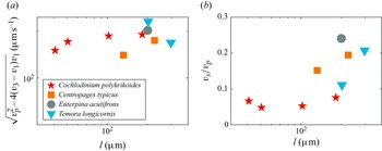


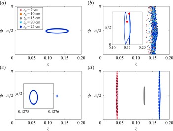


 Open access

