


1. Introduction
Locomotion of microorganisms plays vital roles in various biological processes, including reproduction, foraging and biofilm formation (Fauci & Dillon Reference Fauci and Dillon2006; Lauga Reference Lauga2016). Artificial microswimmers that move like their biological counterparts also show great promise for different biomedical applications such as drug delivery and microsurgery (Nelson, Kaliakatsos & Abbott Reference Nelson, Kaliakatsos and Abbott2010; Sengupta, Ibele & Sen Reference Sengupta, Ibele and Sen2012; Li et al. Reference Li, Esteban-Fernández de Ávila, Gao, Zhang and Wang2017). For their fundamental biological importance and potentially transformative applications, there have been growing interdisciplinary efforts in recent years to better understand the locomotion of these biological and artificial microswimmers (Moran & Posner Reference Moran and Posner2017; Hu, Pané & Nelson Reference Hu, Pané and Nelson2018; Wu et al. Reference Wu, Chen, Mukasa, Pak and Gao2020; Tsang et al. Reference Tsang, Demir, Ding and Pak2020a). These microswimmers employ a variety of mechanisms to overcome the dominance of viscous over inertial forces for self-propulsion at low Reynolds numbers. Extensive studies have shed light on the hydrodynamics of swimming microorganisms (Lauga & Powers Reference Lauga and Powers2009; Yeomans, Pushkin & Shum Reference Yeomans, Pushkin and Shum2014; Elgeti, Winkler & Gompper Reference Elgeti, Winkler and Gompper2015), which has also contributed to the development of various biomimetic or bioinspired artificial swimmers (Bente et al. Reference Bente, Codutti, Bachmann and Faivre2018; Fu et al. Reference Fu, Wei, Yin, Yao and Wang2021). More recently, there has also been a growing interest in exploring the application of machine learning in designing artificial microswimmers (Colabrese et al. Reference Colabrese, Gustavsson, Celani and Biferale2017; Schneider & Stark Reference Schneider and Stark2019; Cichos et al. Reference Cichos, Gustavsson, Mehlig and Volpe2020; Tsang et al. Reference Tsang, Tong, Nallan and Pak2020b; Hartl et al. Reference Hartl, Hübl, Kahl and Zöttl2021; Liu et al. Reference Liu, Zou, Tsang, Pak and Young2021; Muiños-Landin et al. Reference Muiños-Landin, Fischer, Holubec and Cichos2021).
Many microorganisms utilize one or more flexible appendages called flagella and cilia (short flagella) for locomotion. For instance, some spermatozoa of eukaryotic cells swim by propagating bending waves travelling along their flagellum. Colonies of flagellates such as Volvox (Goldstein Reference Goldstein2015) and ciliates such as Paramecium and Tetrahymena have their surface covered by arrays of cilia beating in a coordinated manner. Lighthill (Reference Lighthill1952) and Blake (Reference Blake1971) first studied ciliary propulsion with the squirmer model, where the motion of closely packed cilia tips is represented by distribution of slip velocities on a spherical squirmer surface. In addition to representing specific ciliated microorganisms, the distribution of slip velocity can be adjusted to present different types of swimmers. Based on the representation by Lighthill (Reference Lighthill1952) and Blake (Reference Blake1971), the slip velocity is decomposed into a series of Legendre polynomials, where the coefficients of the series are associated with Stokes flow singularity solutions (Ghose & Adhikari Reference Ghose and Adhikari2014; Pak & Lauga Reference Pak and Lauga2014; Pedley Reference Pedley2016). The first mode of the decomposition corresponds to a source dipole and accounts for the swimming of the organism, and the second mode corresponds to a force dipole that characterizes the type of the swimmer. Many studies considered these two squirming modes to represent pushers and pullers, which obtain their thrust from, respectively, the rear (e.g. Escherichia coli) and front (e.g. Chlamydomonas) part of their body. The squirmer model has therefore become a widely used generic locomotion model for various problems in low-Reynolds-number swimming, including nutrient uptake by microorganisms (Magar, Goto & Pedley Reference Magar, Goto and Pedley2003; Magar & Pedley Reference Magar and Pedley2005; Michelin & Lauga Reference Michelin and Lauga2011; Eastham & Shoele Reference Eastham and Shoele2020), optimization (Michelin & Lauga Reference Michelin and Lauga2010), hydrodynamic interactions (Ishikawa, Simmonds & Pedley Reference Ishikawa, Simmonds and Pedley2006; Drescher et al. Reference Drescher, Leptos, Tuval, Ishikawa, Pedley and Goldstein2009), collective motion (Ishikawa & Pedley Reference Ishikawa and Pedley2007; Ishikawa, Simmonds & Pedley Reference Ishikawa, Simmonds and Pedley2007), inertial effects (Wang & Ardekani Reference Wang and Ardekani2012; Chisholm et al. Reference Chisholm, Legendre, Lauga and Khair2016) and swirling motion (Pedley, Brumley & Goldstein Reference Pedley, Brumley and Goldstein2016; Binagia et al. Reference Binagia, Phoa, Housiadas and Shaqfeh2020; Nganguia et al. Reference Nganguia, Zheng, Chen, Pak and Zhu2020; Housiadas Reference Housiadas2021; Housiadas, Binagia & Shaqfeh Reference Housiadas, Binagia and Shaqfeh2021), among others (Pedley Reference Pedley2016).
Of particular recent interest is the use of the squirmer model to probe the impact of non-Newtonian rheology on swimming (Zhu et al. Reference Zhu, Do-Quang, Lauga and Brandt2011; Zhu, Lauga & Brandt Reference Zhu, Lauga and Brandt2012; Montenegro-Johnson, Smith & Loghin Reference Montenegro-Johnson, Smith and Loghin2013; De Corato, Greco & Maffettone Reference De Corato, Greco and Maffettone2015; Datt et al. Reference Datt, Zhu, Elfring and Pak2015; Binagia et al. Reference Binagia, Phoa, Housiadas and Shaqfeh2020; Housiadas et al. Reference Housiadas, Binagia and Shaqfeh2021). Most biological fluids display non-Newtonian rheological behaviours, including viscoelasticity and shear-thinning viscosity. While extensive studies focused on the effect of fluid elasticity (Elfring & Lauga Reference Elfring and Lauga2015; Sznitman & Arratia Reference Sznitman and Arratia2015; Li, Lauga & Ardekani Reference Li, Lauga and Ardekani2021), recent studies have revealed how shear-thinning rheology can also affect locomotion in substantial and non-trivial ways (Lauga Reference Lauga2015; Montenegro-Johnson Reference Montenegro-Johnson2017). The impact of shear-thinning rheology varies among different types of swimmers and the details of their swimming gaits: while the propulsion speed of undulatory (Vélez-Cordero & Lauga Reference Vélez-Cordero and Lauga2013; Gagnon, Keim & Arratia Reference Gagnon, Keim and Arratia2014; Li & Ardekani Reference Li and Ardekani2015; Gagnon & Arratia Reference Gagnon and Arratia2016) and helical (Gómez et al. Reference Gómez, Godínez, Lauga and Zenit2017; Demir et al. Reference Demir, Lordi, Ding and Pak2020; Qu & Breuer Reference Qu and Breuer2020) swimmers can be enhanced significantly, all two-mode squirmers (pushers, pullers or neutral squirmers) swim slower in a shear-thinning fluid (Montenegro-Johnson et al. Reference Montenegro-Johnson, Smith and Loghin2013; Datt et al. Reference Datt, Zhu, Elfring and Pak2015); it is noteworthy that speed enhancement is possible for squirmers with other squirming modes in the slip velocity (Datt et al. Reference Datt, Zhu, Elfring and Pak2015; Pietrzyk et al. Reference Pietrzyk, Nganguia, Datt, Zhu, Elfring and Pak2019). In addition, shear-thinning rheology can render ineffective swimming gaits in a Newtonian fluid (e.g. reciprocal motion) useful in a non-Newtonian fluid (Qiu et al. Reference Qiu, Lee, Mark, Morozov, Münster, Mierka, Turek, Leshansky and Fischer2014; Han et al. Reference Han, Shields IV, Bharti, Arratia and Velev2020). Collectively, these studies demonstrate the profound impact of shear-thinning rheology on low-Reynolds-number locomotion.
In this work, we extend the spherical squirmer model to examine the effect of particle geometry on swimming in a shear-thinning fluid. While the squirmer model by Lighthill (Reference Lighthill1952) and Blake (Reference Blake1971) may be adequate for spherically shaped organisms like Volvox, swimmers with non-spherical shapes are commonly found in nature. To better represent ciliates such as Paramecium and Tetrahymena (see figure 1a) and, more generally, to probe the effect of geometrical shape upon ciliary locomotion, Keller & Wu (Reference Keller and Wu1977) generalized the squirmer model to a prolate spheroidal body of arbitrary eccentricity. The theoretical prediction of streamlines in their spheroidal model found good agreement with experimental streak photographs of freely swimming and inert sedimenting Paramecium caudatum. The original spheroidal squirmer model by Keller & Wu (Reference Keller and Wu1977) includes only the swimming mode without a force-dipole mode, which has been incorporated into the model by more recent studies (Ishimoto & Gaffney Reference Ishimoto and Gaffney2013; Theers et al. Reference Theers, Westphal, Gompper and Winkler2016; Pöhnl, Popescu & Uspal Reference Pöhnl, Popescu and Uspal2020) to represent other types of swimmers. In addition to representing ciliates with spheroidal bodies, the spheroidal model serves as a first approximation to other non-spherical swimmers (e.g. E. coli) to assess how geometrical shape affects swimming performance. Here, we extend the analysis to the non-Newtonian regime and probe the role of particle geometry on swimming in a shear-thinning fluid via the spheroidal squirmer model. A combined theoretical and numerical framework is used to quantify the impact on both the speed and the energetic cost of swimming. The results reveal key features that are distinct from the spherical case, suggesting the possibility for biological and artificial microswimmers to tune their geometrical shape for improving their swimming performance in complex fluids.
(a) An image of ciliate Tetrahymena thermophila. Image courtesy of Brian Bayless, Santa Clara University/Bayless Lab. (b) The geometrical set-up of a squirmer with a prolate spheroidal body, where  $a$ and
  $b$ are, respectively, the semi-major and semi-minor axes. The unit normal
  $\boldsymbol {n}=\boldsymbol {e}_\tau$ and tangent
  $\boldsymbol {s}=-\boldsymbol {e}_\zeta$ vectors to the spheroidal surface
  $S$ are expressed in terms of the basis vectors in the prolate spheroidal coordinates.

This paper is organized as follows. We formulate the problem in § 2 by introducing the prolate spheroidal squirmer model, the governing equations, and the rheological constitutive model employed in this work. In § 3, we present the asymptotic analysis and numerical simulations used to quantify the locomotion of a spheroidal squirmer in a shear-tinning fluid. Results on the swimming speed, power dissipation and swimming efficiency, as well as their implications for the design of artificial microswimmers, are discussed in § 4. Finally, we conclude this work with closing remarks in § 5.
2. Problem formulation
2.1. Geometrical set-up
We use a spheroidal squirmer model to examine the effect of geometrical shape on locomotion in a shear-thinning fluid. Since many ciliates such as Paramecium and Tetrahymena have prolate spheroidal bodies (see figure 1a), we focus on the locomotion of a prolate spheroidal squirmer in this work for its biological relevance. See figure 1(b) for notations and geometrical set-up. The equation describing the surface of the prolate spheroidal body reads
 \begin{equation} \frac{z^{2}}{a^{2}} + \frac{r^{2}}{b^{2}} =1, \end{equation}
where  $r^{2} = x^{2}+y^{2}$,
  $a$ is the semi-major axis, and
  $b\le a$ is the semi-minor axis. The spheroidal coordinate system that we use is given by
  $(\tau,\zeta,\phi )$, where
  $1\leqslant \tau \leqslant \infty$,
  $-1\leqslant \zeta \leqslant 1$ and
  $0\leqslant \phi \leqslant 2 {\rm \pi}$. The position vector is given by
 \begin{equation} \boldsymbol{x} = c \sqrt{\tau^{2}-1} \sqrt{1-\zeta^{2}} \,\boldsymbol{e}_r + c\tau\zeta \,\boldsymbol{e}_z, \end{equation}
where  $\boldsymbol {e}_r = \cos {\phi } \, \boldsymbol {e}_x + \sin {\phi } \,\boldsymbol {e}_y$,
  $c=\sqrt {a^{2}-b^{2}}$ is half of the focal length, and
  $e=c/a$ is the eccentricity. Here, we define
  $\tau _0=1/e$, with
  $\tau > \tau _0$ corresponding to the fluid domain exterior to the surface (
 $\tau =\tau _0$) of the squirmer. The unit vectors of the prolate spheroidal coordinates
  $\boldsymbol {e}_\tau$ and
  $\boldsymbol {e}_\zeta$ are related to those of the Cartesian coordinates as
 \begin{equation} \boldsymbol{e}_\tau = \frac{\tau\sqrt{1-\zeta^{2}}}{\sqrt{\tau^{2}-\zeta^{2}}}\,\boldsymbol{e}_r+\frac{\zeta\sqrt{\tau^{2}-1}}{\sqrt{\tau^{2}-\zeta^{2}}}\,\boldsymbol{e}_z, \quad \boldsymbol{e}_\zeta ={-}\frac{\zeta\sqrt{\tau^{2}-1}}{\sqrt{\tau^{2}-\zeta^{2}}}\,\boldsymbol{e}_r+\frac{\tau\sqrt{1-\zeta^{2}}}{\sqrt{\tau^{2}-\zeta^{2}}}\,\boldsymbol{e}_z. \end{equation}
The metric coefficients for the prolate spheroidal coordinates are given by
 \begin{equation} h_{\tau} = c\,\frac{\sqrt{\tau^{2}-\zeta^{2}}}{\sqrt{\tau^{2}-1}}, \quad h_{\zeta} = c\,\frac{\sqrt{\tau^{2}-\zeta^{2}}}{\sqrt{1-\zeta^{2}}}, \quad h_{\phi} = c\sqrt{1-\zeta^{2}}\sqrt{\tau^{2}-1}. \end{equation}
The unit normal and tangent vectors on the spheroidal surface are given by the basis vectors, respectively, as  $\boldsymbol {n}=\boldsymbol {e}_\tau$ and
  $\boldsymbol {s}=-\boldsymbol {e}_\zeta$.
2.2. The squirmer model
Similar to the spherical squirmer model (Lighthill Reference Lighthill1952; Blake Reference Blake1971), surface velocities are prescribed on a prolate spheroidal squirmer to represent the effect of the ciliary motion on the fluid. Following Keller & Wu (Reference Keller and Wu1977), a steady tangential velocity distribution of the form  $\boldsymbol {u}^{S} = -B_1 (\boldsymbol {s} \boldsymbol {\cdot } \boldsymbol {e}_z) \boldsymbol {s}$ is prescribed on the squirmer surface
  $S$ (figure 1b). In the spherical limit,
  $\boldsymbol {s} \rightarrow \boldsymbol {e}_\theta$, and the squirming velocity reduces to the first mode
  $\boldsymbol {u}^{S} = B_1 \sin \theta \,\boldsymbol {e}_\theta$ considered by Lighthill (Reference Lighthill1952) and Blake (Reference Blake1971). Subsequent studies have included additional modes of surface velocities (Ishimoto & Gaffney Reference Ishimoto and Gaffney2013; Theers et al. Reference Theers, Westphal, Gompper and Winkler2016; Eastham & Shoele Reference Eastham and Shoele2020; Pöhnl et al. Reference Pöhnl, Popescu and Uspal2020). In particular, Theers et al. (Reference Theers, Westphal, Gompper and Winkler2016) included the contribution of a force-dipole as a second mode (
 $B_2$) in the form
 \begin{align} \boldsymbol{u}^{S} &={-}B_1 (\boldsymbol{s} \boldsymbol{\cdot} \boldsymbol{e}_z ) \boldsymbol{s} - B_2 \zeta (\boldsymbol{s}\boldsymbol{\cdot} \boldsymbol{e}_z) \boldsymbol{s} \end{align}
 \begin{align} &={-}B_1\tau_0(1+ \alpha \zeta) \sqrt{\frac{1-\zeta^{2}}{\tau_0^{2}-\zeta^{2}}} \, \boldsymbol{e_{\zeta}}, \end{align}
where the sign of the ratio  $\alpha = B_2/B_1$ represents a pusher (
 $\alpha <0$) or puller (
 $\alpha >0$), and the case
  $\alpha =0$ corresponds to a neutral squirmer. The two-mode spheroidal squirmer reduces to the spherical model by Lighthill (Reference Lighthill1952) and Blake (Reference Blake1971) in the limit of zero eccentricity (
 $e=0$). Here, we extend previous analyses on spherical squirmers in a shear-thinning fluid (Montenegro-Johnson et al. Reference Montenegro-Johnson, Smith and Loghin2013; Datt et al. Reference Datt, Zhu, Elfring and Pak2015) and examine the effect of particle geometry via the spheroidal squirmer model given by (2.6).
2.3. Governing equations
The momentum and continuity equations in the limit of low Reynolds number are, respectively, given by
 $$\begin{gather} \boldsymbol{\nabla} \boldsymbol{\cdot} \boldsymbol{\sigma} = \boldsymbol{0}, \end{gather}$$
 $$\begin{gather}\boldsymbol{\nabla} \boldsymbol{\cdot} \boldsymbol{u} = 0, \end{gather}$$
where  $\boldsymbol {\sigma } = -p \boldsymbol{\mathsf{I}} + \boldsymbol{\mathsf{T}}$,
  $p$ is the pressure,
  $\boldsymbol{\mathsf{I}}$ is the identity tensor, and
  $\boldsymbol{\mathsf{T}}$ is the deviatoric stress tensor. To capture the reduction in the viscosity due to increased shear rates in a shear-thinning fluid, we use the Carreau constitutive equation (Bird, Armstrong & Hassanger Reference Bird, Armstrong and Hassanger1987), where
 \begin{equation} \boldsymbol{\mathsf{T}} = [ \mu_{\infty}+(\mu_0-\mu_{\infty})(1+\lambda^{2}| \dot{\boldsymbol{\gamma}} |^{2})^{(n-1)/2}] \dot{\boldsymbol{\gamma}}. \end{equation}
Here,  $\mu _0$ and
  $\mu _\infty$ are, respectively, the zero and infinite shear rate viscosities, and the strain rate tensor
  $\dot {\boldsymbol {\gamma }}=\boldsymbol {\nabla } \boldsymbol {u}+(\boldsymbol {\nabla } \boldsymbol {u})^{\rm T}$ has magnitude
  $|\dot {\boldsymbol {\gamma }}|=(\dot {\gamma }_{ij}\dot {\gamma }_{ij}/2)^{1/2}$. The power-law index
  $n<1$ characterizes the degree of shear-thinning, and
  $1/\lambda$ characterizes the critical shear rate at which the non-Newtonian behaviour becomes significant. The Carreau model has been shown to be effective in describing the rheological behaviours of different biological fluids, and has been employed in previous studies of locomotion in a shear-thinning fluid (Montenegro-Johnson et al. Reference Montenegro-Johnson, Smith and Loghin2013; Vélez-Cordero & Lauga Reference Vélez-Cordero and Lauga2013; Datt et al. Reference Datt, Zhu, Elfring and Pak2015; Li & Ardekani Reference Li and Ardekani2015; Nganguia et al. Reference Nganguia, Zheng, Chen, Pak and Zhu2020).
In the laboratory frame, the flow decays to zero in the far field
 \begin{equation} \boldsymbol{u}(\tau\rightarrow\infty,\zeta) = \boldsymbol{0}, \end{equation}
and the boundary condition on the surface of the squirmer is given by
 \begin{equation} \boldsymbol{u}(\tau=\tau_0,\zeta) = \boldsymbol{u}^{S}+\boldsymbol{U}, \end{equation}
where the squirming velocity distribution  $\boldsymbol {u}^{S}$ given by (2.6) causes the squirmer to translate with an unknown swimming velocity
  $\boldsymbol {U}$. The system is closed by enforcing the force-free condition
 \begin{equation} \int_S \boldsymbol{n} \boldsymbol{\cdot} \boldsymbol{\sigma} \, \text{d}S = \boldsymbol{0}, \end{equation}
where  $\boldsymbol {n} = \boldsymbol {e}_{\tau }$ is the unit normal vector on the squirmer surface. We note that the axisymmetric velocity distribution in (2.6) does not induce any rotational velocity and the squirmer is torque-free. By symmetry, swimming occurs in the
  $z$-direction,
  $\boldsymbol {U}= U \boldsymbol {e}_z$.
We non-dimensionalize the problem by scaling lengths by  $a$, velocities by
  $B_1$, strain rates by
  $\omega = B_1/a$, and stresses by
  $\mu _0 \omega$. The dimensionless momentum and continuity equations are given by, respectively,
  $\boldsymbol {\nabla } \boldsymbol {\cdot } \boldsymbol {\sigma }^{*}=\boldsymbol {0}$ and
  $\boldsymbol {\nabla } \boldsymbol {\cdot } \boldsymbol {u}^{*}=0$, where the stars
  $(^{*})$ denote dimensionless variables. The deviatoric stress tensor
  $\boldsymbol{\mathsf{T}}^{*}$ takes a dimensionless form
 \begin{equation} \boldsymbol{\mathsf{T}}^{*} = [ \beta+(1-\beta)(1+Cu^{2}| \dot{\boldsymbol{\gamma}}^{*} |^{2})^{(n-1)/2}] \dot{\boldsymbol{\gamma}}^{*}, \end{equation}
where the Carreau number  $Cu = \omega \lambda$ compares the characteristic strain rate
  $\omega$ to the critical strain rate
  $1/\lambda$, and the viscosity ratio
  $\beta = \mu _{\infty }/\mu _0$ compares the zero and infinite shear rate viscosities. Both dimensionless groups measure the extent of the shear-thinning effect. Hereafter we refer only to dimensionless variables and therefore drop the stars for convenience.
3. Asymptotic analysis and numerical simulations
3.1. Asymptotic analysis
The Carreau constitutive equation (2.13) reduces to the Newtonian constitutive equation when  $Cu=0$ or
  $\beta =1$. We can therefore examine the weakly non-Newtonian behaviour by expanding variables in the limits of small
  $Cu$ (
 $\varepsilon = Cu^{2} \ll 1$) or small deviation of
  $\beta$ from unity (
 $\varepsilon = 1-\beta \ll 1$) in perturbation series
 \begin{equation} \left\{\boldsymbol{u},\boldsymbol{\sigma},\boldsymbol{\mathsf{T}},\dot{\boldsymbol{\gamma}},\boldsymbol{U} \right\} = \left\{\boldsymbol{u}_0,\boldsymbol{\sigma}_0,\boldsymbol{\mathsf{T}}_0,\dot{\boldsymbol{\gamma}}_0,\boldsymbol{U}_0 \right\} + \varepsilon \left\{\boldsymbol{u}_1,\boldsymbol{\sigma}_1,\boldsymbol{\mathsf{T}}_1,\dot{\boldsymbol{\gamma}}_1,\boldsymbol{U}_1 \right\} + O(\varepsilon^{2}). \end{equation}
The zeroth-order solution corresponds to the flow around a spheroidal squirmer in a Newtonian fluid, which satisfies
 $$\begin{gather} \boldsymbol{\nabla}\boldsymbol{\cdot} \boldsymbol{\sigma}_{0} = \boldsymbol{0}, \end{gather}$$
 $$\begin{gather}\boldsymbol{\nabla} \boldsymbol{\cdot} \boldsymbol{u}_{0} = 0, \end{gather}$$
where  $\boldsymbol {\sigma }_{0} = -p_0 \boldsymbol{\mathsf{I}} + \dot {\boldsymbol {\gamma }}_0$ and
  $\dot {\boldsymbol {\gamma }}_0 = \boldsymbol {\nabla } \boldsymbol {u}_0 + (\boldsymbol {\nabla } \boldsymbol {u}_0)^{\rm T}$. The boundary condition on the squirmer surface is given by
  $\boldsymbol {u}_0 (\tau = \tau _0, \zeta ) = \boldsymbol {u}^{S}+ \boldsymbol {U}_0$, and the flow decays to zero in the far field. The Newtonian solution was obtained in previous analyses (Keller & Wu Reference Keller and Wu1977; Theers et al. Reference Theers, Westphal, Gompper and Winkler2016; Pöhnl et al. Reference Pöhnl, Popescu and Uspal2020). In terms of streamfunction
  $\psi _0$ in prolate spheroidal coordinates, where
 \begin{equation} \boldsymbol{u}_0 = \frac{1}{h_\zeta h_\phi}\,\frac{\partial \psi_0}{\partial \zeta}\, \boldsymbol{e}_{\tau} - \frac{1}{h_\tau h_\phi}\,\frac{\partial \psi_0}{ \partial \tau}\, \boldsymbol{e}_{\zeta}, \end{equation}
the solution is given by
 \begin{equation} \psi_{0} = C_1\,H_2(\tau)\,G_2(\zeta)+C_2 \tau (1-\zeta^{2})+C_3\,H_3(\tau)\,G_3(\zeta)+ C_4 \zeta(1-\zeta^{2}), \end{equation}
where  $G_n(x)$ and
  $H_n(x)$ are, respectively, the Gegenbauer functions of the first and second kind of degree
  $-1/2$, and the coefficients are determined as
 \begin{equation} \left.\begin{gathered} C_1 = \frac{2 U_0(\tau_0^{2}+1)-4 \tau_0^2}{\tau_0^{2}[(\tau_0^{2}+1)\coth^{{-}1}{\tau_0}-\tau_0]}, \quad C_2 = \frac{ \tau_0\left[\tau_0-(\tau_0^{2}-1)\coth^{{-}1}{\tau_0}\right]-U_0}{\tau_0^{2}[(\tau_0^{2}+1)\coth^{{-}1}{\tau_0}-\tau_0]}, \\ C_3 = \frac{4\alpha }{\tau_0[3\tau_0+(1-3\tau_0^{2})\coth^{{-}1}\tau_0]}, \quad C_4 = \frac{\alpha \left[2/3-\tau_0^{2}+\tau_0(\tau_0^{2}-1)\coth^{{-}1}\tau_0 \right]}{\tau_0[3\tau_0+(1-3\tau_0^{2})\coth^{{-}1}\tau_0]} . \end{gathered}\right\} \end{equation}
Upon enforcing the force-free condition (2.12), the swimming speed of a spheroidal squirmer in a Newtonian fluid is equal to (Keller & Wu Reference Keller and Wu1977; Theers et al. Reference Theers, Westphal, Gompper and Winkler2016)
 \begin{equation} U_{0} = \tau_0[\tau_0-(\tau_0^{2}-1)\coth^{{-}1}{\tau_0}]. \end{equation}
 At  $O(\varepsilon )$, the momentum and continuity equations are, respectively, given by
 $$\begin{gather} \boldsymbol{\nabla} \boldsymbol{\cdot} \boldsymbol{\sigma}_1 = \boldsymbol{0}, \end{gather}$$
 $$\begin{gather}\boldsymbol{\nabla} \boldsymbol{\cdot} \boldsymbol{u}_1 = 0, \end{gather}$$
where  $\boldsymbol {\sigma }_1 = -p_1\boldsymbol{\mathsf{I}} + \boldsymbol{\mathsf{T}}_1$ and the first non-Newtonian correction to the deviatoric stress is
  $\boldsymbol{\mathsf{T}}_{1} = \dot {\boldsymbol {\gamma }}_{1} + \boldsymbol{\mathsf{A}}$; here, the tensor
  $\boldsymbol{\mathsf{A}}$ depends on the choice of the asymptotic limit,
  $\varepsilon = Cu^{2}$ or
  $\varepsilon = 1-\beta$. Expanding (2.13) with
  $\varepsilon = Cu^{2}$ gives
 \begin{equation} \boldsymbol{\mathsf{A}} = \frac{(1-\beta)(n-1)}{2}\,| \dot{\boldsymbol{\gamma}}_0 |^{2} \dot{\boldsymbol{\gamma}}_0, \end{equation}
whereas expanding (2.13) with  $\varepsilon = 1-\beta$ gives
 \begin{equation} \boldsymbol{\mathsf{A}} = \left[{-}1+(1+Cu^{2}| \dot{\boldsymbol{\gamma}}_0 |^{2})^{(n-1)/2}\right] \dot{\boldsymbol{\gamma}}_0. \end{equation}
We consider results in both asymptotic limits in the following sections.
To obtain the first non-Newtonian correction to the swimming speed  $\boldsymbol {U}_1$, we use the Lorentz reciprocal theorem (Stone & Samuel Reference Stone and Samuel1996; Lauga Reference Lauga2014; Elfring Reference Elfring2017; Masoud & Stone Reference Masoud and Stone2019) to bypass solving (3.8) and (3.9) for the first-order flow,
  $(\boldsymbol {u}_1, p_1)$. To apply the reciprocal theorem, we consider an auxiliary Stokes flow problem of the same geometry, satisfying
 $$\begin{gather} \boldsymbol{\nabla}\boldsymbol{\cdot} \hat{\boldsymbol{\sigma}} = \boldsymbol{0}, \end{gather}$$
 $$\begin{gather}\boldsymbol{\nabla}\boldsymbol{\cdot} \hat{\boldsymbol{u}} = 0, \end{gather}$$
where  $\hat {\boldsymbol {\sigma }}= -\hat {p} \boldsymbol{\mathsf{I}}+ \boldsymbol {\nabla } \hat {\boldsymbol {u}}+ (\boldsymbol {\nabla } \hat {\boldsymbol {u}})^\textrm {T}$. From (3.8) and (3.12), we take the inner products between the flow fields and the divergence of the stress fields in the auxiliary and first-order problems to obtain the relation
 \begin{equation} \hat{\boldsymbol{u}}\boldsymbol{\cdot}(\boldsymbol{\nabla} \boldsymbol{\cdot} \boldsymbol{\sigma}_1)=\boldsymbol{u}_1 \boldsymbol{\cdot}(\boldsymbol{\nabla} \boldsymbol{\cdot} \hat{\boldsymbol{\sigma}}) = 0. \end{equation}
With the identity  $\hat {\boldsymbol {u}}\boldsymbol {\cdot }(\boldsymbol {\nabla } \boldsymbol {\cdot } \boldsymbol {\sigma }_1)-\boldsymbol {u}_1 \boldsymbol {\cdot }(\boldsymbol {\nabla } \boldsymbol {\cdot } \hat {\boldsymbol {\sigma }}) = \boldsymbol {\nabla } \boldsymbol {\cdot } (\hat {\boldsymbol {u}} \boldsymbol {\cdot } \boldsymbol {\sigma }_1 - \boldsymbol {u}_1\boldsymbol {\cdot } \hat {\boldsymbol {\sigma }}) + (\boldsymbol {\nabla }\boldsymbol {u}_1 \boldsymbol{:} \hat {\boldsymbol {\sigma }}-\boldsymbol {\nabla } \hat {\boldsymbol {u}} \boldsymbol{:} \boldsymbol {\sigma }_1)$, we integrate (3.14) over the fluid volume and use the divergence theorem to obtain
 \begin{equation} \int_S{\boldsymbol{n}\boldsymbol{\cdot}\hat{{\boldsymbol{\sigma}}}\boldsymbol{\cdot}{\boldsymbol{u}}_1} \,\text{d}S - \int_S{\boldsymbol{n}\boldsymbol{\cdot}{\boldsymbol{\sigma}}_1 \boldsymbol{\cdot}{\hat{\boldsymbol{u}}}} \,\text{d}S=\int_V{\boldsymbol{\sigma}_1\boldsymbol{:}\boldsymbol{\nabla}\hat{\boldsymbol{u}}}\,\text{d}V- \int_V{\hat{\boldsymbol{\sigma}}\boldsymbol{:}\boldsymbol{\nabla}\boldsymbol{u}_1} \,\text{d}V. \end{equation}
By substituting the expression of the stresses  $\hat {\boldsymbol {\sigma }}$ and
  $\boldsymbol {\sigma }_1$ in the auxiliary and first-order problems into the right-hand side of (3.15), we obtain
 \begin{equation} \int_S{\boldsymbol{n}\boldsymbol{\cdot}\hat{{\boldsymbol{\sigma}}}\boldsymbol{\cdot}{\boldsymbol{u}}_1} \,\text{d}S - \int_S{\boldsymbol{n}\boldsymbol{\cdot}{\boldsymbol{\sigma}}_1 \boldsymbol{\cdot}{\hat{\boldsymbol{u}}}} \,\text{d}S=\int_V{\boldsymbol{\mathsf{A}}\boldsymbol{:}\boldsymbol{\nabla}\hat{\boldsymbol{u}}}\, \text{d}V. \end{equation}
In order to determine  $\boldsymbol {U}_{1}$, we choose the auxiliary Stokes flow problem to be the flow due to the translation of a prolate spheroid with velocity
  $\hat {\boldsymbol {U}}$ (Happel & Brenner Reference Happel and Brenner1965). The relation (3.16) thus becomes
 \begin{equation} \hat{\boldsymbol{F}} \boldsymbol{\cdot} \boldsymbol{U}_1 - \boldsymbol{F}_1 \boldsymbol{\cdot} \hat{\boldsymbol{U}} =\int_V{\boldsymbol{\mathsf{A}}\boldsymbol{:}\boldsymbol{\nabla}\hat{\boldsymbol{u}}}\,\text{d}V, \end{equation}
where  $\hat {\boldsymbol {F}}=\int _S \boldsymbol {n} \boldsymbol {\cdot } \hat {\boldsymbol {\sigma }} \,\textrm {d}S = -8{\rm \pi} \hat {\boldsymbol {U}}/\tau _0[(\tau _0^{2}+1)\coth ^{-1}\tau _0-\tau _0]$ is the force experienced by a translating spheroid in the auxiliary problem. By enforcing the force-free condition (2.12) at
  $O(\varepsilon )$,
  $\boldsymbol {F}_1=\int _S \boldsymbol {n}\boldsymbol {\cdot } \boldsymbol {\sigma }_1 \,\textrm {d}S = \boldsymbol {0}$, the reciprocal theorem gives the final result
 \begin{equation} \hat{\boldsymbol{F}} \boldsymbol{\cdot} \boldsymbol{U}_1 =\int_V{\boldsymbol{\mathsf{A}}\boldsymbol{:}\boldsymbol{\nabla}\hat{\boldsymbol{u}}}\,\text{d}V, \end{equation}
where only two known Stokes flow solutions, namely the zeroth-order ( $\boldsymbol {u}_0$) and auxiliary (
 $\hat {\boldsymbol {u}}$) problems, are required to determine the non-Newtonian swimming velocity
  $\boldsymbol {U}_1$.
In addition to the first-order swimming velocity, the reciprocal theorem can be applied to obtain the first-order power dissipation when considering the energetic cost of squirming through a shear-thinning fluid (Nganguia, Pietrzyk & Pak Reference Nganguia, Pietrzyk and Pak2017), which we will examine in more detail in § 4.2.
3.2. Numerical simulations
To compare with the results from the asymptotic analysis, we also perform fully coupled numerical simulations of the momentum and continuity equations (2.7) and (2.8), together with the Carreau constitutive equation (2.9), using the finite element method implemented in the COMSOL Multiphysics environment. To take advantage of the axial symmetry of the problem, an axisymmetric computational domain in the  $r$–
$r$– $z$ plane is used to simulate only half of the full flow domain. The squirmer is modelled as a half spheroid whose major axis coincides with the axis of symmetry. To simulate the locomotion of a squirmer in an unbounded fluid, we ensure that the computational domain (of size
  $500a \times 500a$) is sufficiently large so that the numerical results are independent of the size of the domain. We perform the simulations in a reference frame moving with the squirmer, which leads to a uniform flow in the far field as the inflow boundary condition. The magnitude of the inflow is equal to the unknown swimming speed of the squirmer, which is obtained by solving the momentum and continuity equations simultaneously, with the force-free swimming condition (2.12) as a global equation. A zero pressure is specified for the outflow boundary condition.
  $\textrm {P}2+\textrm {P}1$ discretization is applied to the flow field: namely, second-order elements are used for the velocity components, and first-order elements are used for the pressure. Triangular mesh elements are used for the simulations, with local mesh refinement near the squirmer to resolve properly the spatial variation of the viscosity. The degrees of freedom are of the order of
  $1.8\times 10^{5}$ for the simulations. We used PARDISO (the Parallel Direct Solver) for all simulations.
In addition to comparing with the asymptotic results in this work, we have validated our numerical implementation against previous results for both spherical (Lighthill Reference Lighthill1952; Blake Reference Blake1971) and spheroidal (Keller & Wu Reference Keller and Wu1977; Theers et al. Reference Theers, Westphal, Gompper and Winkler2016) squirmers in a Newtonian fluid, as well as spherical squirmers in a shear-thinning fluid (Datt et al. Reference Datt, Zhu, Elfring and Pak2015).
4. Results and discussion
4.1. Swimming speed
We use results from both the asymptotic analysis and numerical simulations to examine the effect of particle geometry on squirming through a shear-thinning fluid. We first consider the small Carreau number limit,  $\varepsilon = Cu^{2}$, by substituting the expression (3.10) into (3.18) to obtain the swimming speed in a shear-thinning fluid as
 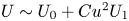 $U\sim U_0+Cu^{2} U_1$. The Newtonian speed
  $U_0$ is given by (3.7), and the first non-Newtonian correction reads
 \begin{equation} U_1=\frac{(1-\beta)(n-1)}{2} \left[\sum_{i=0}^{3} \gamma_i(\tau_0) + \alpha^{2} \chi(\tau_0) \sum_{i=0}^{7} \delta_i(\tau_0) \right], \end{equation}
where  $\gamma _i(\tau _0)$,
  $\delta _i(\tau _0)$ and
  $\chi (\tau _0)$ are constants depending on
  $\tau _0$; their expressions are given in Appendix A. Figure 2(a) shows the results from the asymptotic analysis (lines) given by (4.1) and numerical simulations (symbols). The asymptotic result (4.1) reveals that the propulsion speed varies linearly with
  $1-\beta$ and
  $n-1$; in numerical simulations we set
  $n=0.25$ for its relevance to biological mucus (Hwang, Litt & Forsman Reference Hwang, Litt and Forsman1969; Vélez-Cordero & Lauga Reference Vélez-Cordero and Lauga2013). Previous studies (Montenegro-Johnson et al. Reference Montenegro-Johnson, Smith and Loghin2013; Datt et al. Reference Datt, Zhu, Elfring and Pak2015) found that cylindrical and spherical squirmers with the first two modes (pushers, pullers and neutral squirmers) swim consistently slower in a shear-thinning fluid (
 $U/U_0<1$). Interestingly, the asymptotic analysis reveals that it is possible for a spheroidal squirmer to swim faster in a shear-thinning fluid than in a Newtonian fluid (
 $U/U_0>1$; figure 2a): for a neutral squirmer (
 $\alpha =0$), enhanced swimming occurs when
 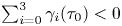 $\sum _{i=0}^{3} \gamma _i(\tau _0)<0$, which can be solved numerically to obtain a critical eccentricity,
  $e_c \approx 0.81$, above which a spheroidal squirmer swims at a speed higher than its Newtonian value, as shown in figure 2(a). For a pusher/puller (
 $\alpha \neq 0$), an increase in the magnitude of
  $\alpha$ acts to reduce the swimming speed in the small
  $Cu$ limit. Figure 2(b) maps the regimes where enhanced (
 $U/U_0>1$) and hindered (
 $U/U_0<1$) swimming occur in this asymptotic limit. The critical value of
  $\alpha$ is determined from (4.1) as
 \begin{equation} \alpha_c = \sqrt{\frac{-\displaystyle\sum_{i=0}^{3} \gamma_i(\tau_0)} {\chi(\tau_0) \displaystyle\sum_{i=0}^{7} \delta_i(\tau_0)}}, \end{equation}
for different values of the eccentricity (solid line, figure 2b). We note that the above result is independent of  $\beta$ and
  $n$, which appear only in the prefactor in the asymptotic expression (4.1). We also remark that the quadratic dependence on
  $\alpha$ in (4.1) shows that the swimming speed does not depend on the sign of
  $\alpha$ (i.e. a pusher versus a puller), which still holds beyond the asymptotic regime considered here, as shown by numerical simulations (see Appendix B for more details). While the sign of
  $\alpha$ does not affect the swimming speed, the detailed velocity and pressure fields surrounding a squirmer depend on both the magnitude and sign of
  $\alpha$.
(a) Swimming speed of a spheroidal squirmer  $U$ in a shear-thinning fluid relative to its corresponding Newtonian value
  $U_0$ as a function of eccentricity
  $e$ for different values of viscosity ratio
  $\beta$. Here,
  $\alpha =0$,
  $n=0.25$ and
  $Cu=0.1$. Both asymptotic (lines) and numerical (symbols) results predict that enhanced swimming (
 $U/U_0\geqslant 1$) occurs when the eccentricity exceeds a critical value
  $e_c \approx 0.81$. (b) For a pusher/puller (
 $\alpha \neq 0$), the
  $\alpha$–
 $e$ diagram maps the regimes where enhanced (
 $U/U_0>1$) and hindered (
 $U/U_0<1$) swimming occur.

To examine the dependence of swimming speed over a full range of  $Cu$, we consider the other asymptotic limit,
  $\varepsilon =1-\beta$, and use (3.11) in the integral theorem (3.18). Figure 3(a) displays different types of non-monotonic variations with
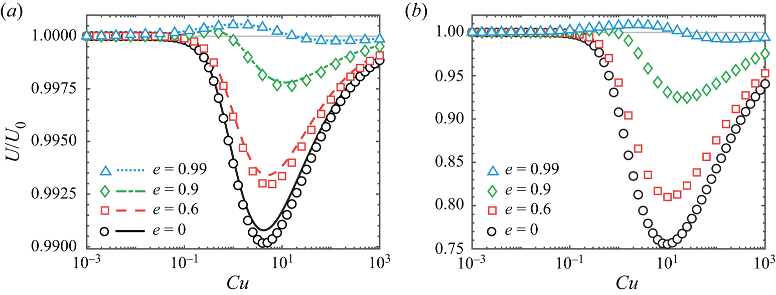
  $Cu$ in this asymptotic limit, depending on the value of eccentricity. Here, we focus on the results for neutral squirmers (
 $\alpha =0$); the results for pushers (
 $\alpha <0$) and pullers (
 $\alpha >0$) can be obtained in a similar fashion (see Appendix B). For a spherical squirmer (
 $e=0$) and a spheroidal squirmer with an eccentricity below the critical value (
 $e=0.6 < e_c$), the swimming speed first decays with increased
  $Cu$, reaching a local minimum before approaching the Newtonian value as
  $Cu$ continues to increase. However, for squirmers with eccentricities above the critical value (
 $e>e_c \approx 0.81$; e.g.
  $e=0.9$ and
  $0.99$ in figure 3a), the speed first increases with
  $Cu$, attaining a local maximum speed that is faster than the corresponding Newtonian value before approaching the Newtonian value at larger values of
  $Cu$. We note that the seemingly minute variations are merely consequences of the use of small parameters in the asymptotic analysis. In figure 3(b) we verify through numerical simulations with
  $\beta =0.1$ that these features remain the same beyond the weakly non-Newtonian regime; the speed variations are substantially larger compared with the asymptotic results. These results highlight the importance of particle geometry on swimming in a shear-thinning fluid: while shear-thinning rheology acts to retard the motion of a spherical squirmer, increasing the eccentricity (or slenderness) of the particle helps to mitigate the speed reduction generally; moreover, the speed could even be enhanced relative to the Newtonian value at certain values of
  $Cu$ when the eccentricity is above the critical value. In particular, it is noteworthy that a spheroidal squirmer with
  $e=0.99$ has only relatively minute variations of swimming speed over a wide range of
  $Cu$, as shown in figure 3. This feature illustrates the possibility of designing a spheroidal swimmer that can restore effectively the substantial loss of swimming speed due to shear-thinning viscosity in the spherical case. Such a robust performance is especially desirable for swimmers that need to traverse complex media with vastly varying rheological properties.
(a) Swimming speed of a spheroidal squirmer  $U$ in a shear-thinning fluid relative to its corresponding Newtonian value
  $U_0$ as a function of
  $Cu$ for different values of eccentricity
  $e$ when
  $\beta = 0.9$. The asymptotic results in the small
  $\varepsilon =1-\beta$ limit (lines) agree well with numerical simulations (symbols). An increased value of eccentricity enhances the swimming speed in general. For values of eccentricity above the critical value (e.g.
  $e=0.9$ and
  $0.99$), the squirmer can swim faster in a shear-thinning fluid than in a Newtonain fluid. The qualitative behaviours remain the same beyond the weakly non-Newtonian regime when
  $\beta =0.1$ as shown by numerical simulations in (b); we also note the substantially larger speed variations in (b). In both (a,b),
  $\alpha =0$ and
  $n=0.25$.
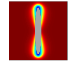
In figure 4, we examine the distributions of flow speed, pressure and viscosity around a spheroidal squirmer with different eccentricities obtained by numerical simulations. As the eccentricity increases, the variations of flow speed (figure 4a), pressure (figure 4b) and viscosity (figure 4c) all become increasingly localized at the poles of the squirmer. In particular, the viscosity distributions in figure 4(c) provide some insights that may help us to understand the observed dependence of propulsion speed on the squirmer geometry. For a spherical squirmer, the viscosity reduction in a shear-thinning fluid is fairly uniform around the squirmer, as shown in figure 4(c) ( $e=0$). The physical scenario may therefore be akin to a squirmer immersed in a low-viscosity inner fluid surrounded by a high-viscosity outer fluid. Such a confinement effect was shown to reduce the propulsion speed of the squirmer (Reigh & Lauga Reference Reigh and Lauga2017), consistent with the speed reduction of a spherical squirmer in a shear-thinning fluid. When the squirmer becomes more eccentric, the viscosity reduction becomes more non-uniform, with the reduction concentrating around the poles and diminished reduction near the equator. Such localization of viscosity reduction disrupts the uniform confinement effect in the spherical case, contributing plausibly to the increasingly restored propulsion speed in a shear-thinning fluid as the squirmer becomes more spheroidal. As shown in figure 4(c), the localization is particularly apparent for a highly eccentric squirmer (
 $e=0.99$), which indeed can swim faster in a shear-thinning fluid than in a Newtonian fluid, in stark contrast to the case of a spherical squirmer.
Distributions of (a) flow speed  $|\boldsymbol {u}|$, (b) pressure
  $p$, and (c) viscosity
  $\mu$ around a spheroidal squirmer with different eccentricities in the co-moving frame in a shear-thinning fluid. From left to right, the eccentricity is
  $e=0$, 0.6, 0.9 and 0.99. Here,
  $\alpha =0$,
  $\beta =0.1$,
  $Cu=10^{0.4}$ and
  $n=0.25$.

As a remark, the (soft) confinement effect may have qualitatively different consequences on the propulsion of different types of swimmers. In particular, the enhanced propulsion of undulatory (Li & Ardekani Reference Li and Ardekani2015; Riley & Lauga Reference Riley and Lauga2017) and helical (Gómez et al. Reference Gómez, Godínez, Lauga and Zenit2017; Demir et al. Reference Demir, Lordi, Ding and Pak2020) swimmers was attributed to the soft confinement effect, which could instead cause the speed reduction of a spherical squirmer (Reigh & Lauga Reference Reigh and Lauga2017). The results on spheroidal squirmers here further illustrate how the effect may manifest differently depending on the particle geometry, highlighting this subtle and significant factor in understanding locomotion in a shear-thinning fluid.
4.2. Power dissipation and swimming efficiency
We next consider the effect of particle geometry on the energetic cost of squirming through a shear-thinning fluid. We calculate the power  $\mathcal {P}$ expended by the squirmer during the swimming process, which is equal to the power dissipation in the fluid:
 \begin{equation} \mathcal{P} ={-}\int_S \boldsymbol{n} \boldsymbol{\cdot} \boldsymbol{\sigma} \boldsymbol{\cdot} \boldsymbol{u} \,\text{d}S. \end{equation}
Here, we focus on results for a neutral squirmer; contributions from other modes can be calculated in a similar fashion. We expand  $\mathcal {P}$ in the asymptotic limit of small
  $\varepsilon$,
 \begin{equation} \mathcal{P} = \mathcal{P}_0 + \varepsilon \mathcal{P}_1 + O(\varepsilon^{2}), \end{equation}
where the Newtonian power dissipation is given by Keller & Wu (Reference Keller and Wu1977) as
 \begin{equation} \mathcal{P}_{0} = \frac{4{\rm \pi}(\tau_0^{2}-1)\left[(1+\tau_0^{2})\coth^{{-}1}{\tau_0}-\tau_0\right]}{\tau_0}, \end{equation}
and the first non-Newtonian correction is given by  $\mathcal {P}_1 = - \int _S \boldsymbol {n} \boldsymbol {\cdot }\boldsymbol {\sigma }_{1} \boldsymbol {\cdot } \boldsymbol {u}_{0} \, \textrm {d}S - \int _S \boldsymbol {n} \boldsymbol {\cdot } \boldsymbol {\sigma }_{0} \boldsymbol {\cdot } \boldsymbol {u}_{1} \,\textrm {d}S$. By applying the boundary condition
  $\boldsymbol {u}_{1} = \boldsymbol {U}_{1}$ on the squirmer surface, the second integral in
  $\mathcal {P}_1$ becomes
  $\int _S \boldsymbol {n} \boldsymbol {\cdot } \boldsymbol {\sigma }_{0} \,\textrm {d}S \boldsymbol {\cdot } \boldsymbol {U}_{1}$, which vanishes due to the force-free condition
  $\int _S \boldsymbol {n} \boldsymbol {\cdot } \boldsymbol {\sigma }_{0} \,\textrm {d}S = \boldsymbol {0}$. The first non-Newtonian correction to the power dissipation is therefore given by
 \begin{equation} \mathcal{P}_1 ={-} \int_S \boldsymbol{n} \boldsymbol{\cdot} \boldsymbol{\sigma}_{1} \boldsymbol{\cdot} \boldsymbol{u}_{0} \,{\rm d}S. \end{equation}
We can again bypass the calculation of the first-order stress  $\boldsymbol {\sigma }_1$ and obtain
  $\mathcal {P}_1$ via the reciprocal theorem (3.16) by choosing an appropriate auxiliary problem. Specifically, here we choose the auxiliary problem to be the zeroth-order (or Newtonian) flow around a spheroidal squirmer (Keller & Wu Reference Keller and Wu1977):
  $(\hat {p}, \hat {\boldsymbol {u}})=(p_0, \boldsymbol {u}_0)$. The integral relation (3.16) hence becomes
 \begin{equation} \int_S {\boldsymbol{n} \boldsymbol{\cdot} \boldsymbol{\sigma}}_0 \boldsymbol{\cdot} \boldsymbol{u}_1 \, \text{d}S - \int_S \boldsymbol{n} \boldsymbol{\cdot} \boldsymbol{\sigma}_1 \boldsymbol{\cdot} {\boldsymbol{u}}_0 \, \text{d}S = \int_V \boldsymbol{\mathsf{A}} \boldsymbol{:} \boldsymbol{\nabla} {\boldsymbol{u}}_0 \,{\rm d}V, \end{equation}
where the first integral on the left-hand side vanishes,  $\int _S {\boldsymbol {n} \boldsymbol {\cdot } \boldsymbol {\sigma }}_0 \boldsymbol {\cdot } \boldsymbol {u}_1 \,\textrm {d}S = \int _S {\boldsymbol {n} \boldsymbol {\cdot } \boldsymbol {\sigma }}_0 \,\textrm {d}S \boldsymbol {\cdot } \boldsymbol {U}_1 = 0$, due to the boundary condition
  $\boldsymbol {u}_1 =\boldsymbol {U}_1$ on
  $S$ and the force-free condition
  $\int _S {\boldsymbol {n} \boldsymbol {\cdot } \boldsymbol {\sigma }}_0 \,\textrm {d}S = \boldsymbol {0}$. The reciprocal theorem therefore allows us to express (4.6) as (De Corato et al. Reference De Corato, Greco and Maffettone2015; Nganguia et al. Reference Nganguia, Pietrzyk and Pak2017)
 \begin{equation} \mathcal{P}_{1} = \int_V \boldsymbol{\mathsf{A}} \boldsymbol{:} \boldsymbol{\nabla}\boldsymbol{u}_{0} \,{\rm d}V. \end{equation}
We use quadrature to calculate the power dissipation from (4.8) for a wide range of  $Cu$ in the small
  $\varepsilon = 1-\beta$ limit. Figure 5(a) displays results from the asymptotic analysis and numerical simulations, which both show that the power dissipation decreases with
  $Cu$ in general. In addition, an increased eccentricity further reduces the energetic cost of squirming through a shear-thinning fluid. We verify by numerical simulations that the same trends hold beyond the weakly non-Newtonian regime in figure 5(b).
(a) Power dissipation of a spheroidal squirmer  $\mathcal {P}$ in a shear-thinning fluid relative to its corresponding Newtonian value
  $\mathcal {P}_0$ as a function of
  $Cu$ for different values of eccentricity
  $e$ when
  $\beta =0.9$. The asymptotic results in the small
  $\varepsilon =1-\beta$ limit (lines) agree well with numerical simulations (symbols). The qualitative behaviours remain the same beyond the weakly non-Newtonian limit when
  $\beta = 0.1$, as shown by numerical simulations in (b). In both (a,b),
  $\alpha =0$ and
  $n=0.25$. While the behaviours are qualitatively similar in (a,b), we note the substantially larger variations in (b).

Next, we use the power dissipation to calculate the efficiency of swimming through a shear-thinning fluid. Lighthill (Reference Lighthill1975) introduced the Froude efficiency, a concept borrowed from propeller theory, to characterize the efficiency of swimming at low Reynolds numbers. The swimming efficiency is defined as
 \begin{equation} \eta = \frac{\tilde{\mathcal{P}}}{\mathcal{P}}, \end{equation}
which compares the power expended by the squirmer swimming in the shear-thinning fluid,  $\mathcal {P}$, to the power required to tow a particle of the same geometry at the same swimming speed,
  $\tilde {\mathcal {P}}$. The power in the towing problem is given by
  $\tilde {\mathcal {P}} = \tilde {\boldsymbol {F}} \boldsymbol {\cdot } \boldsymbol {U}$, where
  $\tilde {\boldsymbol {F}}$ is the force required to tow a rigid spheroid at the swimming velocity
  $\boldsymbol {U}$ in the same shear-thinning fluid. We calculate the efficiency asymptotically (De Corato et al. Reference De Corato, Greco and Maffettone2015; Nganguia et al. Reference Nganguia, Pietrzyk and Pak2017) as
 \begin{equation} \eta = \eta_0+\varepsilon \eta_1 + O(\varepsilon^{2}). \end{equation}
The zeroth-order (Newtonian) value is given by Keller & Wu (Reference Keller and Wu1977) as  $\eta _{0}= 2\tau _0^{2}[\tau _0+(1-\tau _0^{2})\coth ^{-1}{\tau _0}]^{2}/(\tau _0^{2}-1)[\tau _0-(1+\tau _0^{2})\coth ^{-1}{\tau _0}]^{2}$, and the first-order correction
  $\eta _1$ is calculated with asymptotic expansions of
  $\mathcal {P} \sim \mathcal {P}_0 + \varepsilon \mathcal {P}_1$ and
  $\tilde {\mathcal {P}} \sim \tilde {\mathcal {P}}_{0} + \varepsilon \tilde {\mathcal {P}}_{1}$. The expansion of the towing power is given by
 \begin{equation} \tilde{\mathcal{P}} = \tilde{\boldsymbol{F}}_0 \boldsymbol{\cdot} \boldsymbol{U}_0 + \varepsilon (\tilde{\boldsymbol{F}}_1 \boldsymbol{\cdot} \boldsymbol{U}_0+ \tilde{\boldsymbol{F}}_0 \boldsymbol{\cdot} \boldsymbol{U}_1) + O(\varepsilon^{2}), \end{equation}
which involves expansions of the swimming velocity  $\boldsymbol {U} \sim \boldsymbol {U}_0 + \varepsilon \boldsymbol {U}_1$ and towing force
  $\tilde {\boldsymbol {F}} \sim \tilde {\boldsymbol {F}}_0 +\varepsilon \tilde {\boldsymbol {F}}_1$, where the first-order corrections to both quantities are again determined by the reciprocal theorem (Datt et al. Reference Datt, Zhu, Elfring and Pak2015; Nganguia et al. Reference Nganguia, Pietrzyk and Pak2017). Figure 6(a) displays the asymptotic results for swimming efficiency in the small
  $\varepsilon = 1-\beta$ limit (lines), which agree well with results by full numerical simulations (symbols). First, the swimming efficiency is enhanced generally relative to the Newtonian case,
  $\eta /\eta _0>1$. Second, for a given eccentricity, there exists an optimal value of
  $Cu$ that maximizes the swimming efficiency. Finally, the maximum swimming efficiency attainable increases with the eccentricity. We verify by numerical simulations that the same trends hold beyond the weakly non-Newtonian regime in figure 6(b); when the viscosity is
  $\beta = 0.1$, an eccentricity of
  $e=0.99$ allows the swimming efficiency to be enhanced significantly by almost 80 % relative to the Newtonian efficiency in a shear-thinning fluid. We also remark that, unlike propulsion speed, there is no qualitative change in terms of propulsion efficiency below or above the critical eccentricity; the squirmer consistently propels more efficiently in a shear-thinning fluid for all eccentricities considered.
(a) Swimming efficiency of a spheroidal squirmer  ${\eta }$ in a shear-thinning fluid relative to its corresponding Newtonian value
  ${\eta }_0$ as a function of
  $Cu$ for different values of eccentricity
  $e$ when
  $\beta =0.9$. The asymptotic results in the small
  $\varepsilon =1-\beta$ limit (lines) agree well with numerical simulations (symbols). The qualitative behaviours remain the same beyond the weakly non-Newtonian limit when
  $\beta = 0.1$, as shown by numerical simulations in (b). In both (a,b),
  $\alpha =0$ and
  $n=0.25$. While the behaviours are qualitatively similar in (a,b), we note the substantially larger variations in (b).

Overall, the asymptotic and numerical results presented here demonstrate that a spheroidal squirmer can swim both faster (§ 4.1) and more efficiently (this subsection) compared with its spherical counterpart in a shear-thinning fluid.
5. Conclusion
Biological and artificial microswimmers often need to traverse biological fluids with complex rheological properties. In particular, shear-thinning viscosity is a ubiquitous non-Newtonian fluid behaviour of many biological fluids, which can impact swimming in substantial and non-trivial ways. Via a spherical squirmer model, previous works showed that shear-thinning viscosity can lead to substantial loss of swimming speed compared with swimming in a Newtonian fluid. In this work, we extend these previous analyses and consider a spheroidal squirmer to probe the effect of particle geometry on the performance of swimming in a shear-thinning fluid. Through asymptotic analysis and numerical simulations, our results show that by increasing its eccentricity, a spheroidal squirmer can effectively restore the loss of swimming speed in a shear-thinning fluid. Indeed, when the eccentricity exceeds a critical value, the spheroidal squirmer can swim faster in a shear-thinning fluid than in a Newtonian fluid, a feature in stark contrast to the corresponding cases of spherical squirmers. As a particular example, we demonstrate that a spheroidal squirmer with a large eccentricity can have a robust swimming performance over a wide range of Carreau numbers, a feature particularly desirable for swimmers that need to traverse environments with vastly varying properties. In addition to the swimming speed, the energetic cost of swimming through a shear-thinning fluid reduces with an increased eccentricity. The swimming efficiency of a spheroidal squirmer can be enhanced substantially as a result.
Taken together, the results here demonstrate the advantages of spheroidal over spherical swimmers in terms of locomotion performance in a shear-thinning fluid, which call for comparisons with future experiments with biological and artificial microswimmers. Recent studies have shed light on optimal swimming of non-spherical swimmers in a Newtonian fluid (Guo et al. Reference Guo, Zhu, Liu, Bonnet and Veerapaneni2021; Daddi-Moussa-Ider et al. Reference Daddi-Moussa-Ider, Nasouri, Vilfan and Golestanian2021). The findings here suggest the possibility and hence opportunity of fine-tuning the swimmer geometry to better exploit non-Newtonian rheological behaviours for more effective locomotion in complex fluids.
Funding
We acknowledge the National Science Foundation for funding support under CBET-1931292 and EFMA-1830958 (to O.S.P.). Computations were performed using the WAVE computing facility at Santa Clara University, enabled by the Wiegand Foundation.
Declaration of interests
The authors report no conflict of interest.
Author contributions
B.v.G and E.D. contributed equally to this work.
Appendix A
In this appendix, we list the expressions for the constants in the swimming speed given by (4.1) in the small Carreau number limit. The constants associated with the  $B_1$ squirming mode are given by
 $$\begin{gather} \gamma_0 = \frac{1}{\tau_0(\tau_0^{2}-1)} \sum_{k=0}^{7}D_k^{0}\tau_0^{2k+1}, \end{gather}$$
 $$\begin{gather}\gamma_1 = \frac{(\tau_0^{2}-1)\coth^{{-}1}\tau_0}{\tau_0}\sum_{k=0}^{6}D_k^{1}\tau_0^{2k}, \end{gather}$$
 $$\begin{gather}\gamma_2 = \frac{(\tau_0^{2}-1)^{3}(\coth^{{-}1}\tau_0)^{2}}{\tau_0}\sum_{k=0}^{1}D_k^{2}\tau_0^{2k+6}, \end{gather}$$
 $$\begin{gather}\gamma_3 = \frac{\lambda(\tau_0^{2}-1)^{3}}{\tau_0} \sum_{k=0}^{1}D_k^{3}\tau_0^{2k+6}, \end{gather}$$
where  $\lambda ={Li}_2[(1-\tau _0)/(1+\tau _0)]+{\rm \pi} ^{2}/12-2\ln [(2\tau _0)/(1+\tau _0)]\coth ^{-1}\tau _0$,
  ${Li}_2(x)$ is the dilogarithm function of the variable
  $x$, and the values of
  $D_k^{i}$ are given in table 1.


The constants associated with the  $B_2$ squirming mode are given by
 $$\begin{gather} \chi = \frac{1}{\left[(3\tau_0^{2}-1)\coth^{{-}1}{(\tau_0)}-3\tau_0\right]^{2}}, \end{gather}$$
 $$\begin{gather}\delta_0 = \frac{1}{\tau_0^{2}-1}\sum_{k=0}^{5}E_k^{0}\tau_0^{2k+4}, \end{gather}$$
 $$\begin{gather}\delta_1 = \frac{ \coth^{{-}1}\tau_0}{\tau_0^{2}-1}\sum_{k=0}^{6}E_k^{1}\tau_0^{2k+3}, \end{gather}$$
 $$\begin{gather}\delta_2 = \frac{(\coth^{{-}1}\tau_0)^{2}}{\tau_0^{2}-1}\sum_{k=0}^{14}E_k^{2}\tau_0^{k+2}, \end{gather}$$
 $$\begin{gather}\delta_3 = (\tau_0^{2}-1)(\coth^{{-}1}\tau_0)^{3}\sum_{k=0}^{12}E_k^{3}\tau_0^{k+1}, \end{gather}$$
 $$\begin{gather}\delta_4 = (\tau_0^{2}-1)^{2}(\coth^{{-}1}\tau_0)^{4}\sum_{k=0}^{5}E_k^{4}\tau_0^{k+6}, \end{gather}$$
 $$\begin{gather}\delta_5 = \lambda (\tau_0^{2}-1) \sum_{k=0}^{3}E_k^{5}\tau_0^{2k+5}, \end{gather}$$
 $$\begin{gather}\delta_6 = \lambda (\tau_0^{2}-1)\coth^{{-}1}\tau_0 \sum_{k=0}^{3}E_k^{6}\tau_0^{2k+6}, \end{gather}$$
 $$\begin{gather}\delta_7 = \lambda (\tau_0^{2}-1)^{3}(\coth^{{-}1}\tau_0)^{2} \sum_{k=0}^{1}E_k^{7}\tau_0^{2k+7}, \end{gather}$$
where the values of  $E_k^{i}$ are given in table 2.


Appendix B
In this appendix, we remark on the effect of an increased magnitude of  $\alpha$ on the swimming speed for pushers (
 $\alpha <0$) and pullers (
 $\alpha >0$) beyond the weakly non-Newtonian regime discussed in the main text. Figure 7 displays results from numerical simulations when
  $\alpha =0$,
  $\pm 0.5$ and
  $\pm 1$ for a spheroidal squirmer with eccentricity
  $e=0.6$ (figure 7a) and
  $e=0.9$ (figure 7b). These values of eccentricity are chosen to capture the two distinct scenarios when a neutral spheroidal squirmer (
 $\alpha =0$) could swim slower (
 $e=0.6$; figure 7a) and faster (
 $e=0.9$; figure 7b) than its Newtonian speed in a shear-thinning fluid. In both cases, the qualitative behaviours of increasing the magnitude of
  $\alpha$ are similar. First, the asymptotic result (4.1) predicts that the swimming speed is independent of the sign of
  $\alpha$ at small
  $Cu$. Consistent with the asymptotic result, pushers and pullers have the same swimming speeds in a shear-thinning fluid even beyond the asymptotic regime, when the shear-thinning effect becomes more substantial. Second, the swimming speed decays generally with an increased magnitude of
  $\alpha$ in the small
  $Cu$ regime, as the asymptotic analysis suggests. More complex variations with
  $\alpha$ occur at larger values of
  $Cu$, and the speed can grow with the magnitude of
  $\alpha$; nevertheless, the speed is still smaller than the corresponding value in a Newtonian fluid. Overall, an increased magnitude of
  $\alpha$ is found to reduce the local minimum speeds in both figures 7(a) and 7(b), as well as the local maximum speed that appears when
  $\alpha =0$ in figure 7(b).
Swimming speed of a spheroidal squirmer  $U$ in a shear-thinning fluid relative to its corresponding Newtonian value
  $U_0$ for different values of
  $\alpha$ when (a)
  $e=0.6$ and (b)
  $e=0.9$. Consistent with the asymptotic results, numerical simulations here show that pushers (
 $\alpha <0$) and pullers (
 $\alpha >0$) have indistinguishable swimming speeds in a shear-thinning fluid. In both (a,b),
  $n=0.25$ and
  $\beta =0.1$.
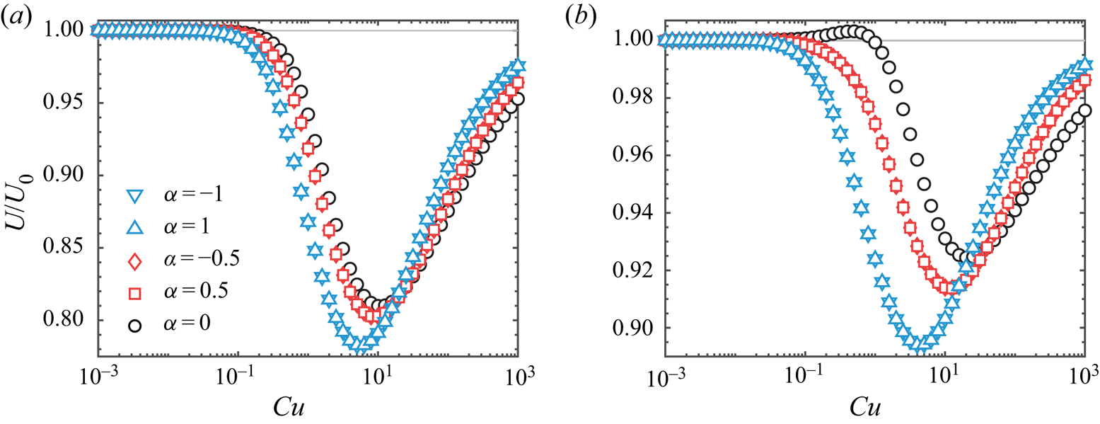


 Open access