


Impact Statement
Surface roughness, whose representative element size is comparable to the hydraulic diameter, incurs a significant drag penalty. This large-scale roughness is usually removed in conventional subtractive manufacturing, making small-scale roughness that occupies a few per cent of the boundary layer the rule in fluid engineering. It is therefore not surprising that most rough-wall boundary-layer theories and models are developed for small-scale roughness. The use of new engineering technologies leads to new flow problems, to which conventional theories do not apply. Here, flow in additively manufactured super-rough channels is such a new problem. This paper is the first direct numerical simulation (DNS) study of flows in additively manufactured super-rough channels. We compare our DNS results with the existing theories/models and show where the existing theories and models fail and succeed. In addition to providing benchmark data for a new engineering problem, this work has real-world impacts: a fluid engineer would know from this study which theories and models they can/cannot trust when dealing with large-scale roughness. This work also impacts fundamental research: our findings, e.g. that the logarithmic law of the wall survives large-scale roughness, motivate revisions of the conventional rough-wall boundary-layer theories.
1. Introduction
Surface roughness in conventional fluid engineering is usually small, occupying a few per cent of the boundary layer (Reference Flack and SchultzFlack & Schultz, 2010). Figure 1(a) shows a sketch of a typical rough-wall boundary layer. The boundary layer consists of the roughness sublayer, the logarithmic layer and the wake layer (Reference JiménezJiménez, 2004; Reference Schlichting and GerstenSchlichting & Gersten, 2003). The roughness sublayer extends from the wall to approximately 3 $k$ to 5 $k$, where $k$ is the roughness’ peak to trough height and represents the most important length scale in the roughness sublayer. Fluid in the roughness sublayer directly interacts with the surface roughness, leading to non-negligible mean flow inhomogeneity in the streamwise ( $x$) and spanwise ( $z$) directions. Above the roughness sublayer is the logarithmic layer. Here, we define the logarithmic layer to be the layer where the mean velocity follows the logarithmic law of the wall, and when we say the logarithmic layer survives, we are saying the logarithmic law of the wall survives. The logarithmic layer extends to approximately $0.15\delta$. The roughness affects the logarithmic layer by setting a momentum flux, and the flow is statistically homogeneous in the streamwise and the spanwise directions. The mean flow follows
 \begin{equation} \frac{U}{u_\tau} = \frac{1}{\kappa}\log\left(\frac{y-d}{y_o}\right) \equiv\frac{1}{\kappa}\log((y-d)^ + ) + B-{\rm \Delta} U^ + {\approx} \frac{1}{\kappa}\log\left(\frac{y}{k_s}\right) + 8.5\end{equation}
in the logarithmic layer, where  $U$ is the time-averaged streamwise velocity, $\kappa \approx 0.4$ is the von Kármán constant (Reference Marusic, Monty, Hultmark and SmitsMarusic, Monty, Hultmark, & Smits, 2013), $d$ is the zero-plane displacement height (Reference ThomThom, 1971), $y_o$ is the equivalent roughness height, ${\rm \Delta} U^+$ is the roughness function, $B\approx 5.2$ is a constant, $k_s$ is the equivalent sandgrain roughness height and $u_\tau$ is the friction velocity. Above the logarithmic layer is the wake layer, within which the boundary-layer height $\delta$ is an important length scale. The layered structure in figure 1(a) applies equally to atmospheric boundary layers – although they are not the focus of this work.
(a) The layered structure of a rough-wall boundary layer. Here,  $k$ is the roughness height, $\delta$ is the boundary-layer height. (We reserve the symbol
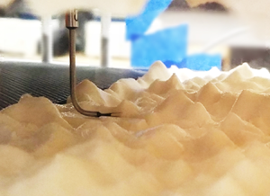
  $h$ for half-channel height.) (b) A spanwise–wall-normal cross-section of an additively manufactured channel (Reference Bons, Taylor, McClain and RivirBons, Taylor, McClain, & Rivir, 2001; Reference McClain, Hanson, Cinnamon, Snyder, Kunz and TholeMcClain et al., 2021). The red and blue lines are the surface roughness; $y_b$ and $y_t$ are the intended bottom- and top-wall locations (when manufacturing the channel); $y_{b-}$ and $y_{t-}$ are the trough locations of the bottom and top surface roughness; $y_{b+}$ and $y_{t+}$ are the peak locations of the bottom and top surface roughness. (c) A sketch of slender roughness. Here, $w$ is the width of the roughness element.

Equation (1.1) has several convenient features. First, it requires no plane average (since the flow in the logarithmic layer is statistically homogeneous in the streamwise and the spanwise directions), and measurements at any streamwise and spanwise location would give the same  $y_o$ and $d$. This is why researchers and engineers can rely on one-dimensional hot-wire measurements in rough-wall boundary-layer experiments (Reference Hultmark, Vallikivi, Bailey and SmitsHultmark, Vallikivi, Bailey, & Smits, 2012; Reference Hutchins, Nickels, Marusic and ChongHutchins, Nickels, Marusic, & Chong, 2009; Reference Örlü, Fiorini, Segalini, Bellani, Talamelli and AlfredssonÖrlü et al., 2017; Reference Wang and ZhengWang & Zheng, 2016). Furthermore, according to (1.1), the effects of surface roughness can be parameterized by $d$ and ${\rm \Delta} U^+$. It follows that roughness modelling is, practically, the modelling of $d$ and ${\rm \Delta} U^+$, and when $d$ is negligible, roughness modelling is the modelling of ${\rm \Delta} U^+$. This simplifies an otherwise complex problem, and (1.1) is the starting point of practically all existing roughness models (Reference Coceal and BelcherCoceal & Belcher, 2004; Reference Flack and SchultzFlack & Schultz, 2010; Reference Forooghi, Stroh, Magagnato, Jakirlić and FrohnapfelForooghi, Stroh, Magagnato, Jakirlić, & Frohnapfel, 2017; Reference Jouybari, Yuan, Brereton and MurilloJouybari, Yuan, Brereton, & Murillo, 2021; Reference Yang, Sadique, Mittal and MeneveauYang, Sadique, Mittal, & Meneveau, 2016).
The above is the conventional view of rough-wall boundary-layer flows. The use of new engineering technologies in fluid engineering applications often gives rise to novel flow problems. In the context of this paper, the new technology is additive manufacturing, the fluid application is internal cooling in turbomachinery and the new flow problem is flow in additively manufactured super-rough cooling channels – channels with surface roughness comparable to their hydrodynamic diameters. In the following, we briefly explain the engineering problem. In more traditional subtractive manufacturing, whatever process is used to machine the channel can be used to finish the surface and remove large-scale roughness. This, however, is often not possible for additively manufactured cooling channels because of the complex geometric designs and the nature of the finishing process. The additive manufacturing process like the one in Reference Stimpson, Snyder, Thole and MongilloStimpson, Snyder, Thole, and Mongillo (2016) gives rise to roughness whose size is approximately 100  $\mathrm {\mu }$m. Since the size of the cooling channel is only approximately 500 $\mathrm {\mu }$m, these additively manufactured roughnesses result in a large drag penalty. This drag penalty must be accounted for in engineering design – giving rise to a new flow problem. Figure 1(b) shows a cross-section of an additively manufactured cooling channel with large-scale roughness on both walls. Here, the cooling channel spans from $y_{b}=0$ to $y_{t}=2h$, the trough to peak height of the top-wall roughness is $|y_{t+}-y_{t-}|=0.8h$ (i.e. $-0.4h< y-y_{t}<0.4h$) and the trough to peak height of the bottom-wall roughness is $|y_{b+}-y_{b-}|=0.34h$ (i.e. $-0.17h< y-y_{b}<0.17h$). Here, $h$ is the intended half-channel height (when manufacturing the channel), $y_{b}$ and $y_{t}$ are the $y$ coordinates of the intended bottom and top surfaces of the channel and the subscripts ‘ $+$’ and ‘ $-$’ denote the peak and trough locations of the surface roughness. The top-wall roughness is larger than the bottom-wall roughness due to the orientation of the surfaces during the manufacturing process (Reference McClain, Hanson, Cinnamon, Snyder, Kunz and TholeMcClain et al., 2021). We have employed the intended half-channel height $h$ as the reference length scale. The reader is directed to Reference Stafford, McClain, Hanson, Kunz and TholeStafford, McClain, Hanson, Kunz, and Thole (2021) for the real dimensions (in millimetres) of the cooling channels and the surface roughness.
Conventional theories like the ones in figure 1(a) do not necessarily apply to new flow problems like the one in figure 1(b). Below, we explain why not. We know that the height of the roughness sublayer is 3 $k$ to 5 $k$. Let us be conservative and assume that the height of the roughness sublayer is 3 $k$. It follows that the top-wall roughness sublayer extends from $y_{t-}$ to $y_{t-}-2.4h$ (the $y$ coordinate points from the bottom wall to the top wall) and the bottom-wall roughness sublayer from $y_{b-}$ to $y_{b-}+1.02h$. These two roughness sublayers overlap, and the flow is nowhere homogeneous in the streamwise and the spanwise directions. If one follows the conventional rough-wall boundary-layer theory to its logical conclusion, one must conclude that the logarithmic layer does not survive, and (1.1) is no longer valid. This poses practical challenges. First, if $U\neq \langle U \rangle$, then measurements at one streamwise and spanwise location are not necessarily a good approximation of the mean (double-averaged) velocity. Here, $\langle \cdot \rangle$ denotes plane average. This casts doubts on the conclusions in Reference Stafford, McClain, Hanson, Kunz and TholeStafford et al. (2021) and Reference McClain, Hanson, Cinnamon, Snyder, Kunz and TholeMcClain et al. (2021), where the authors invoked the conventional wisdom and assumed $U= \langle U \rangle$ when studying flow in an additively manufactured super-rough cooling channel. An objective of this work is to re-evaluate the claims in Reference Stafford, McClain, Hanson, Kunz and TholeStafford et al. (2021) and Reference McClain, Hanson, Cinnamon, Snyder, Kunz and TholeMcClain et al. (2021). We also ask the following practical question: How much averaging is needed in the $x$ and $z$ directions before we can claim $\tilde {U}\approx \langle U \rangle$? Here, $\tilde {\cdot }$ denotes spatial filtration in the $x$ or $z$ direction. Second, it is not clear if $\langle U \rangle$ still follows a logarithmic scaling. In other words, does the logarithmic layer survive large-scale roughness and the resulting mean flow inhomogeneity? Third, it is unknown how the available roughness models like the ones in Reference Flack and SchultzFlack and Schultz (2010) and Reference Yang, Sadique, Mittal and MeneveauYang et al. (2016) work for the large-scale roughness. The objective of this work is to answer or shed some light on these questions. We resort to DNS, which, in spite of its high cost (Reference Choi and MoinChoi & Moin, 2012; Reference Yang and GriffinYang & Griffin, 2021), is the most accurate computational fluid dynamics tool. DNS also gives us access to the flow in the roughness layer, which is usually unavailable in a laboratory experiment.
Before we proceed further, we distinguish the roughness in figure 1(b), i.e. the focus of this work, from the tall slender roughness in figure 1(c) and the ‘obstacle’-type roughness mentioned in Reference JiménezJiménez (2004). Although the roughness in figure 1(c) occupies most of the domain, the boundary layer ‘feels’ only the top part of the roughness. Because of that, the roughness sublayer is thin, and the flow becomes statistically homogeneous in the  $x$ and $z$ directions just slightly above the roughness (Reference CastroCastro, 2007; Reference MacDonald, Ooi, García-Mayoral, Hutchins and ChungMacDonald, Ooi, García-Mayoral, Hutchins, & Chung, 2018; Reference Sharma and García-MayoralSharma & García-Mayoral, 2020). The same is true for a wide range of roughness elements. In Reference Chan, MacDonald, Chung, Hutchins and OoiChan, MacDonald, Chung, Hutchins, and Ooi (2018), the sinusoidal roughness’ trough to peak height is approximately 0.3 $R_0$, and the height of the roughness sublayer is approximately 0.5 $R_0$, i.e. less than $2k$, where $R_0$ is the pipe radius. In Reference Xu, Altland, Yang and KunzXu, Altland, Yang, and Kunz (2021), the cubical roughness’ height is 0.25 $h$, and the roughness sublayer is approximately $0.33h$, i.e. less than $1.5k$, where $h$ is the half-channel height. For these rough surfaces, (1.1) and mean flow universality survive, and the sketch in figure 1(a) is still valid. The roughness considered in this work is also different from obstacle-type roughness. In Reference JiménezJiménez (2004), the term ‘flows over obstacles’ refers to flows with $\delta /k\lesssim 50$. Reference JiménezJiménez (2004) argued that there would be little left of the original wall-flow dynamics in these flows. The discussion in Reference JiménezJiménez (2004) concerns the roughness function, but ‘the original wall-flow dynamics’ should, to a bare minimum, encompass the logarithmic layer (and the related dynamics) and the outer layer similarity (and the related dynamics). Both the logarithmic layer and the outer layer similarity have received much attention since Jimenez's seminal annual review paper. These later studies, however, gave a different picture to the one in Reference JiménezJiménez (2004): the original wall-flow dynamics proves to be applicable to flows with much larger roughness (than $\delta /k\lesssim 50$) (Reference Amir and CastroAmir & Castro, 2011; Reference CastroCastro, 2007; Reference Chan, MacDonald, Chung, Hutchins and OoiChan, MacDonald, Chung, Hutchins, & Ooi, 2015; Reference Xu, Altland, Yang and KunzXu et al., 2021), and ‘flows over obstacles’ lack a unanimous definition. In the most recent annual review, Reference Chung, Hutchins, Schultz and FlackChung, Hutchins, Schultz, and Flack (2021) suggested that the ‘flows over obstacles’ may be defined as flows in which the log-law parameters are not very apparent. We will see in § 3 that log-law parameters are clearly apparent in the additively manufactured super-rough channels, so we prefer not to call these flows ‘flows over obstacles’.
The rest of the paper is organized as follows. We show the detailed numerical settings in § 2. The results are presented in § 3, followed by concluding remarks in § 4.
2. Computational details
2.1 Flow configuration
The simulated geometries are rough-wall channels. Three increasingly rough surfaces are considered, i.e. S1, S2 and S3, which are all computed tomography scans of additively manufactured surfaces, where surface S3 is the most rough and surface S1 is the least rough. Figure 2 shows the height distribution of the surface roughness, and table 1 tabulates the statistics of the roughness. The horizontal size of the rough surfaces is  $L_x\times L_y=14h\times 8.5h$, where $h$ is the intended half-channel height. Further details of the three rough surfaces can be found in Reference McClain, Hanson, Cinnamon, Snyder, Kunz and TholeMcClain et al. (2021), where the three rough surfaces are referred to as up-skin, down-skin and realx102, respectively. The intended channel wall is at $k'\approx 0$. The trough to peak heights are $0.16h$, $0.34h$ and $0.8h$ for S1, S2 and S3, respectively. Although the trough to peak height is often used as a measure of the roughness size (Reference JiménezJiménez, 2004), the statistic is not very reliable because its value is determined by the roughness height at two individual locations. Here, we also report the first-order moment: $Ra/h=0.017$, 0.040, 0.1050 for S1, S2 and S3, and the roughness root-mean-square (r.m.s.): $k_{rms}/h=0.021$, 0.051, 0.134, which are more reliable statistics. The single-point roughness height statistics are close to Gaussian for all three surfaces, see figure 3, and therefore empirical correlations like the one in Reference Flack and SchultzFlack and Schultz (2010) and Reference Flack, Schultz and BarrosFlack, Schultz, and Barros (2020) should, in principle, apply. Figure 4 shows the streamwise-averaged roughness height. We see some variations in the spanwise direction, but they are much smaller than the roughness’ peak to trough height. If we were to repeat this exercise for roughness that consists of streamwise strips, we would see much large spanwise roughness heterogeneity.
The height distribution of the three rough surfaces.  $k'$ is the deviation of the real surface from the intended channel surface.

Rough-wall statistics. Here,  $k_{avg}$ is the average roughness, $R_a$ is the first-order moment, $k_{rms}$ is the r.m.s. of the roughness height, $S_k$ is the skewness, $K_u$ is the Kurtosis, $E_x$ is the effective slope. The average roughness height $k_{avg}$ is measured from the intended rough surface. This is why some values are negative. We keep two significant digits after the decimal point. The reader is directed to Reference Chung, Hutchins, Schultz and FlackChung et al. (2021) for the physical significance (not definition) of these roughness parameters.

The probability density function (PDF) of the roughness height distribution. Here,  $\mu _{k'}$ is the mean roughness height, and $\sigma _{k'}$ is the standard deviation of the roughness height. The black solid line is the standard Gaussian distribution.

Streamwise-averaged roughness height. The black bold lines are the streamwise-averaged roughness height. The two thin black lines show the roughness’ peak and trough locations.

We place each rough surface opposite a flat plate and the other two rough surfaces, leading to six configurations. Table 2 shows the further details of the rough-wall channels. The nomenclature is Ch+[bottom surface]+[top surface], where the bottom/top surface is S1, S2, S3 or smooth (S0). In table 2, we also list the trough and the peak locations of the rough surfaces. The flow is not directly blocked by the surface roughness between  $y_{b+}$ and $y_{t+}$. For conventional small engineering roughness on finished surfaces, $y_{b}\approx y_{b+}\approx y_{b-}$, $y_{t}\approx y_{t+}\approx y_{t-}$ and $y_{t+}-y_{b+}\approx 2h$. For the rough-wall channels considered in this work, $y_{t+}-y_{b+}$ ranges from $1.92h$ in Ch10 (the least rough channel) to $1.34h$ in Ch23 (the most rough channel). We will colour code the results in § 3, as shown in the last column of table 3. In table 3, we also tabulate the aerodynamic properties of the rough surfaces, such as the equivalent roughness height and the location of the virtual wall, which we will discuss in § 3.3.
Details of rough-wall channel configuration. Again,  $y_b$ and $y_t$ are the intended bottom- and top-wall locations and are at $y=0$ and $y=2h$, respectively. That is, $y_b=0$ and $y_t=2h$. The subscript $-$ indicates the trough location, and the subscript $+$ indicates the peak location. ‘Bot. surf.’ is short for bottom surface, and ‘Top surf.’ is short for top surface. S0 is a smooth surface. For a smooth surface, $y_b=y_{b-}=y_{b+}$ and $y_t=y_{t-}=y_{t+}$. We keep two significant digits for the numbers reported here.

Rough surfaces’ aerodynamic properties. Here,  $y_o$ is the equivalent roughness height, $y_d$ is the $y$ coordinate of the virtual wall.

2.2 DNS set-up
We conduct DNSs with two Reynolds numbers, namely  $Re_\tau =180$ and $395$. Here, $Re_\tau =h u_{\tau,b}/\nu$ is the friction Reynolds number, with $\nu$ the kinematic viscosity of the fluid, and $u_{\tau,b}=\sqrt {-({\rm d}p/{{\rm d} x}) h/\rho }$ the bulk friction velocity. Because $|y_{t-}-y_{b-}|>2h$, the above friction Reynolds number is an under-estimate of the conventional Reynolds number, whose definition is $(h-y_{b-})u_\tau /\nu$.
The computational domain size is  $L_x\times L_y\times L_z=14h\times (y_{t-}-y_{b-})\times 8.5h$. Here, $L_y\neq 2h$ because $y_{t/b,-}\neq y_{t/b}$. This computational domain is larger than the ones in, for example, Reference Coceal, Thomas, Castro and BelcherCoceal, Thomas, Castro, and Belcher (2006) and Reference Chung, Chan, MacDonald, Hutchins and OoiChung, Chan, MacDonald, Hutchins, and Ooi (2015), where the roughness is single scale, and a minimum channel suffices. The roughness on an additively manufactured surface is multi-scale, and a large computational domain is needed to sample all the roughness scales as in, for example, Reference Yang and MeneveauYang and Meneveau (2017) and Reference Anderson and MeneveauAnderson and Meneveau (2011). Also, our computational domain matches the experiment in Reference McClain, Hanson, Cinnamon, Snyder, Kunz and TholeMcClain et al. (2021).
Table 4 shows the grid information, where ‘R2’ is for  $Re_\tau =180$ and ‘R4’ for $Re_\tau =395$. Uniform grid spacings are used in the streamwise ( $x$) and the spanwise ( $z$) directions, while a hyperbolic-tangent stretched grid is used in the wall-normal ( $y$) direction following Reference Jelly, Jung and ZakiJelly, Jung, and Zaki (2014) and Reference Wang, Wang and ZakiWang, Wang, and Zaki (2019). The grid must resolve the flow and the roughness. Here, the $x$ and $z$ grids are such that ${\rm \Delta} x^+\times {\rm \Delta} z^+\lesssim 12\times 6$ to resolve the flow (Reference Kim, Moin and MoserKim, Moin, & Moser, 1987; Reference Lee and MoserLee & Moser, 2015; Reference Leonardi and CastroLeonardi & Castro, 2010) and ${\rm \Delta} x\times {\rm \Delta} y\lesssim 0.033 h\times 0.033h$ to resolve the surface roughness (Reference Yuan and PiomelliYuan & Piomelli, 2014). Here, $\varDelta _x$, $\varDelta _y$ and $\varDelta _z$ are the grid spacings in the streamwise, wall-normal and spanwise directions, respectively. Figure 5 shows the premultiplied energy spectra of the surface roughness and the grid cutoff in the $Re_\tau =395$ DNSs. The surface roughness is very well resolved. The wall-normal grid resolution is rather fine, with ${\rm \Delta} y^+ \sim 0.4$ at the wall and ${\rm \Delta} y^+ \sim 3.5$ at the channel centreline. These resolutions are comparable to/finer than those in Reference Moser, Kim and MansourMoser, Kim, and Mansour (1999), and since we will not study high-order statistics, these resolutions are sufficient (Reference Yang, Hong, Lee and HuangYang, Hong, Lee, & Huang, 2021).
Grid information. Here,  $N_x$, $N_y$ and $N_z$ are the grid numbers in the streamwise, wall-normal and spanwise directions, respectively; R2 is for $Re_\tau =180$, and R4 is for $Re_\tau =395$. The two numbers for ${\rm \Delta} y$ are the minimum (at the wall) and maximum (the channel centerline) wall-normal grid spacings.

Premultiplied roughness spectra. The spectra are normalized by their maxima. The blue lines are the  $x$ direction spectra. The yellow lines are the $z$ direction spectra. The vertical lines denote the grid cutoff in the $Re_\tau =395$ DNSs.

We employ the in-house code LESGO for the DNSs. The code solves the incompressible Navier–Stokes equations. A spectral method (with the 3/2 rule for dealiasing) is used for spatial discretization in the  $x$ and $z$ directions, and a second-order finite difference method is used in the $y$ direction. Time advancement uses the second-order Adam–Bashforth method. The code has been extensively used for rough-wall boundary-layer flows (Reference Wang, Li and WangWang, Li, & Wang, 2018; Reference Yang, Sadique, Mittal and MeneveauYang, Sadique, Mittal, & Meneveau, 2015; Reference Zhu and AndersonZhu & Anderson, 2018), but most are large-eddy simulations. A DNS validation of the code can be found in Reference Zhu, Minnick and GaymeZhu, Minnick, and Gayme (2021).
2.3 Statistical convergence
The  $x$-momentum equation reads
 \begin{equation} \frac{{\rm d}}{{\rm d} y}\left(\nu\frac{{\rm d} \langle {U} \rangle }{{\rm d} y}-\langle \overline{u'v'} \rangle - \langle u''v'' \rangle \right)-\frac{1}{\rho} \frac{{\rm d} \langle \bar{p} \rangle }{{\rm d} x}-f = 0, \end{equation}
where  $f$ is the drag force (which is 0 outside the roughness occupied region), ${\rm d}/{{\rm d} x}$ and ${\rm d}/{{\rm d} y}$ are total derivatives in the $x$ and $y$ directions, respectively (streamwise- and spanwise-averaged velocity and stresses are only functions of $y$),
$y$),  $\nu$ is the kinematic viscosity, $p$ is the pressure, $\bar {\cdot }$ denotes time average, $\phi ''=\bar {\phi }-\langle \bar {\phi } \rangle$ and $\phi$ is a generic variable (note that $\overline {\phi ''_1\phi ''_2}\equiv \phi ''_1\phi ''_2$ for any $\phi _1$ and $\phi _2$). The terms on the left-hand side are the viscous diffusion term, the turbulent transport term, the dispersive stress term and the pressure gradient term. Integrating equation (2.1) in the $y$ direction leads to
 \begin{equation} \nu\frac{{\rm d} \langle {U} \rangle }{{\rm d} y}-\langle \overline{u'v'} \rangle -\langle u''v'' \rangle = {\rm Const.} + \frac{1}{\rho}\frac{{\rm d} \langle \bar{p} \rangle }{{\rm d} x} y,\end{equation}
outside the roughness, i.e. a linear function of  $y$ – given statistical convergence. Equation (2.2) is often used to check the statistical convergence of a numerical simulation: a simulation is statistically converged if the sum of the viscous, turbulent and dispersive fluxes is a linear function of $y$ (Reference Oliver, Malaya, Ulerich and MoserOliver, Malaya, Ulerich, & Moser, 2014). Figure 6 shows the terms in (2.2), and a linear total flux is indeed found in our DNSs. In addition to the linear total flux, we observe the following. First, the turbulent flux is by far the most dominant term outside the roughness, and the viscous flux is notable only in the roughness occupied layer and the viscous sublayer. This is distinctly different from flows above a spanwise heterogeneous roughness (Reference Anderson, Li and Bou-ZeidAnderson, Li, & Bou-Zeid, 2015), where the dispersive flux is comparable to the turbulent flux. Also, the terms in (2.2) are not symmetric with respect to the channel centreline. Table 5 tabulates the locations where the total stress is 0, which we denote as $y_{\tau }$, and the distance between $y_{\tau }$ and the virtual wall, which is approximately the intended channel surface, i.e. $y_{b,t}$ (see the discussion in § 3). The distance between $y_{\tau }$ and $y_{b,t}$ in plus units measures the effective Reynolds number and is also reported. We see that a rougher surface leads to a larger distance between $y_\tau$ and the virtual wall, which in turn leads to a larger effective Reynolds number. The effective Reynolds number is between 174 and 616. A more in-depth discussion on the effect of the effective Reynolds number is postponed until § 3.
The momentum budget. The  $x$ axis is from $y_b$ to $y_t$ rather than from $y_{b-}$ to $y_{t-}$. The dashed lines indicate the peak locations of the roughness. Turb, Disp, Visc and Total stand for turbulent flux, dispersive flux, viscous flux and total flux, respectively. Here, normalization is by the bulk friction velocity $u_{\tau,b}=\sqrt {-1/\rho \, {\rm d}\langle \bar {p} \rangle /{{\rm d} x}\,h}$.

Flow statistics. Here,  $y_\tau$ is the location where the total stress is 0; $y_t$ and $y_b$ are the intended top and bottom surfaces. The superscript denotes normalization by $\nu /u_{\tau,b}$.

3. Results
We present the DNS results. We focus on the  $Re_\tau =395$ cases, i.e. R4 cases, and only show the $Re_\tau =180$ results, i.e. R2 results, for comparison purposes. In the discussion below, we adopt the following shorthand Ch[a][b]-R[c] when referring to a DNS calculation; a and b are 1, 2 or 3, and c is 2 or 4. Here, Ch[a][b]-R[c] is the $Re_\tau =c\times 10^2$ channel whose bottom and top surfaces are S[a] and S[b].
3.1 Basic flow phenomenology
Figure 7 shows the contours of the instantaneous and temporally averaged streamwise velocity at distances  $k_b/2$ and $k_t/2$ from the intended bottom and top walls in Ch23-R4, where $k_b=|y_{b+}-y_{b-}|$ and $k_t=|y_{t-}-y_{t+}|$ and are the bottom- and top-wall roughness heights. We see streaks of momentum deficits and momentum excesses in figure 7(a,c) at the two $y$ locations. While some of these streaks are transient, some are locked in the spanwise direction, leading to low and high momentum pathways in the mean flow, as we can see in figure 7(b,d). Similar low and high momentum pathways are often seen above spanwise heterogeneous surface roughness (Reference Anderson, Li and Bou-ZeidAnderson et al., 2015) and large-scale roughness (Reference Nikora, Stoesser, Cameron, Stewart, Papadopoulos, Ouro and FalconerNikora et al., 2019). These are secondary flows of the second kind. In the following, we briefly review the recent literature and explain the differences. The recent literature has given much attention to this kind of secondary flow (Reference Forooghi, Yang and AbkarForooghi, Yang, & Abkar, 2020; Reference Medjnoun, Vanderwel and GanapathisubramaniMedjnoun, Vanderwel, & Ganapathisubramani, 2018; Reference Stroh, Schäfer, Frohnapfel and ForooghiStroh, Schäfer, Frohnapfel, & Forooghi, 2020; Reference Wangsawijaya, Baidya, Chung, Marusic and HutchinsWangsawijaya, Baidya, Chung, Marusic, & Hutchins, 2020; Reference Yang, Xu, Huang and GeYang, Xu, Huang, & Ge, 2019). A well-studied model problem is a half-channel with spanwise alternating low and high roughness on the bottom wall. The mean flow is homogeneous in the streamwise direction, and secondary flows show up as counter-rotating vortices in the spanwise–wall-normal plane, and they typically span the entire channel/half-channel. Their sizes and strengths are, by and large, controlled by the spacing of the roughness and not so much by the roughness height $k$. The secondary flows we see here in Ch23-R4 are somewhat different. First, we do not see apparent spanwise roughness heterogeneity in S1, S2 or S3. Also, we do not see counter-rotating vortices in the spanwise–wall-normal plane. The in-plane motions in figure 8 are weak and rather unorganized. It appears that the flows in figure 7(b,d) are what one would find in a roughness sublayer. The results from the other channel configurations are similar and are not shown here for brevity.
Contours of the instantaneous streamwise velocity in Ch23-R4 (a) at  $y=y_b+k_b/2$ and (c) at $y=y_t-k_t/2$. Contours of the time-averaged streamwise velocity in Ch23-R4 at (b) at $y=y_b+k_b/2$ and (d) at $y=y_t-k_t/2$.

Contours of the time-averaged streamwise velocity at a constant  $x$ location. The arrows show the in-plane motion. For visualization purposes, we show arrows between $y=k_b/2$ and $y=2-k_t/2$ only.

3.2 Mean flow inhomogeneity
It should be clear from figure 8 that measurements at a single spanwise–streamwise location are a poor representation of the double-averaged velocity, i.e.  $\langle U \rangle \not \approx U$. Here, ‘double average’ refers to time and streamwise–spanwise averaging. In this section, we quantify the flow inhomogeneity in the streamwise and spanwise directions and determine what we need to do to get a close approximation of the double-averaged velocity. Figure 9(a–c) compares the hot-wire measurements in Reference McClain, Hanson, Cinnamon, Snyder, Kunz and TholeMcClain et al. (2021) and our DNS data for Ch10, Ch20, Ch30. The experimental hot-wire measurements are taken at a single spanwise–streamwise location but at Reynolds numbers from $O(10^4-10^5)$. The Reynolds numbers are on the high end of what we would see in real-world turbomachinery applications (Reference Han and ChenHan & Chen, 2006; Reference Nourin and AmanoNourin & Amano, 2020). The DNSs give access to the three-dimensional flow field, and we show the variation of the time-averaged velocity in the domain, which is bounded by $\max _{x,y}[U(z)]$ and $\min _{x,y}[U(z)]$. Figure 9(d) shows the variation of the time-averaged velocity in Ch30-R2 and Ch30-R4, i.e. at $Re_\tau =180$ and $Re_\tau =395$. These Reynolds numbers are on the low end of what we would see in the industry. In all, the Reynolds number does not impact the basic flow phenomenology, and we see large mean flow variations at both Reynolds numbers.
Velocity profiles in Ch10-R4, Ch20-R4, Ch30-R4 and Ch30-R2. The symbols in (a–c) are hot-wire measurements at one streamwise–spanwise location (Reference McClain, Hanson, Cinnamon, Snyder, Kunz and TholeMcClain et al., 2021). The shaded regions show the variations of the time-averaged streamwise velocity in the domain. The coloured solid lines are the double-averaged velocities in the R4 DNSs. The light and dark shades in (d) show the variation of the time-averaged velocity in Ch30-R4 and Ch30-R2, respectively. Normalization is by the maximum value of the double-averaged velocity. The vertical dashed lines indicate the peak locations of the surface roughness.

It is interesting to note that there are non-negligible variations of the time-averaged velocity near the top smooth surface in figure 9, as the bottom roughness affects the flow near the top surface. This is consistent with the conventional rough-wall boundary-layer theory. The peak to trough height is  $0.16h$, $0.44h$ and $0.8h$ for the S1, S2 and S3 roughness, respectively. The height of the sublayer is usually 3 to 5 times the roughness’ peak to trough height, giving rise to roughness sublayers that are $0.48h - 0.8h$, $1.32h - 2.2h$ and $2.4h - 4h$ for S1, S2 and S3. The channel height is $2h$. We can therefore expect that the roughness sublayer on one side affects the flow on the other side. Moreover, the two roughness sublayers overlap when we put two rough surfaces opposite to each other. This is what we see in figure 10: the two roughness sublayers overlap, and $\max _{x,y}[U(z)]-\min _{x,y}[U(z)]$ maintains a large value throughout the channel in Ch12, Ch13 and Ch23.
Same as figure 9(a–c) but for Ch12-R4, Ch13-R4 and Ch23-R4.

We can more formally quantify the mean flow's variation by applying the following triple decomposition to the velocity and examining the dispersive stress. The triple decomposition reads (Reference FinniganFinnigan, 2000)
 \begin{equation} u = \langle U \rangle + u'' + u', \end{equation}
where  $u$ is the instantaneous velocity, $\langle U \rangle$ is the double-averaged velocity, $u'$ is the temporal fluctuation at a given spatial location and $u''$ is the spatial variation of the mean flow in the streamwise and spanwise directions. The above triple decomposition may be applied to the other two velocity components, but we are only interested in the streamwise component. The r.m.s. of $u''$ gives a formal quantification of the mean flow variation in the wall-parallel directions. Figure 11 shows $u_{rms}^{\prime\prime+}$ in the vicinity of S1, S2 and S3. Each rough surface appears three times in the six channel configurations, leading to the three lines in figure 11(a–c). We make the following observations. First, the lines do not collapse. The dispersive stress $u_{rms}^{\prime\prime+}$ above a rough surface is visibly affected by the roughness on the opposite wall, particularly when the other rough surface is rougher. Second, the dispersive stress $u_{rms}^{\prime\prime+}$ is non-negligible and is larger above a rougher surface. The value is approximately $u_{rms}^{\prime\prime+}\approx 1$ above S3. If we follow the conventional rough-wall boundary-layer theory, we must conclude that there are no logarithmic layers in these super-rough channels, a topic we will discuss more in § 3.3.
Dispersive stress  $u_{rms}^{\prime\prime+}$ near S1, S2 and S3. The plots cutoff at $y/h=1$ or $\langle U \rangle =\max [\langle U \rangle ]$. Here, normalization is by the friction velocity $u_\tau$.

Here, we discuss how we can get a close approximation of the double-averaged velocity in a laboratory experiment. If only one-dimensional measurements like hot-wire are available, measurements at sufficiently many locations are required to determine the average. If two-dimensional (2-D) measurements are available, like particle image velocimetry (PIV), which has been used in rough-wall boundary-layer experiments (Reference Gul and GanapathisubramaniGul & Ganapathisubramani, 2021; Reference Medjnoun, Rodriguez-Lopez, Ferreira, Griffiths, Meyers and GanapathisubramaniMedjnoun et al., 2021; Reference Talapatra and KatzTalapatra & Katz, 2012), we may be able to take averages directly in a 2-D plane. The 2-D plane may be the streamwise–wall-normal plane or the spanwise–wall-normal plane. Because the measurement window is always limited in a laboratory experiment, a practical question is in which direction is averaging more effective. Figure 12 compares spanwise averaging and streamwise averaging. We average in the  $x$ and $z$ direction at the scale $l_x=14h (=L_x)$ and $l_z=8.5h(=L_z)$ and plot the variation of the averaged velocity in the domain. We see that spanwise averaging is generally more effective than streamwise averaging in reducing mean flow variation both within and outside the roughness-occupied layers. This is not surprising as the velocity correlation decays quickly in the spanwise direction than the streamwise direction, and the same filtration length covers more statistically independent samples in the spanwise direction than the streamwise direction. If we regard the streamwise- or the spanwise-averaged velocity at a single spanwise or streamwise location to be an estimate of the double-averaged velocity, the error in that estimate can be quantified as
 \begin{equation} {Err} = \frac{1}{L_y}\int_{y_{b-}}^{y_{t-}} \left(\max_{z,x}[{\tilde{U}_{l_{x,z}}}^ + ]-\min_{z,x} [{\tilde{U}_{l_{x,z}}}^ + ]\right)\, {{\rm d} y}, \end{equation}
where  $\tilde {\cdot }$ denotes streamwise or spanwise averaging at a scale $l_{x/z}$. This error represents the average width of the shaded region in figure 12, as a function of the averaging scale. Figure 13 shows the error as a function of the averaging length scale. For both streamwise and spanwise averaging, spatial averaging is, in general, more effective in reducing the error for less rough channels, where there is less variation in the mean flow to begin with. However, there are exceptions. For example, streamwise averaging is more effective for Ch23, the rougher channel, than Ch20, the less rough channel. Additionally, we see diminished returns from both streamwise and spanwise averaging, and the error reduces very slowly as the averaging length increases beyond a 1 to 2 half-channel heights. Last, we see spanwise averaging is more effective in reducing the error, which is consistent with figure 12.
Mean velocity. The shades show the variation of the mean velocity when the data are not subjected to any spatial filtration, when the data are subjected to streamwise filtration of  $l_x=14h$ and when the data are subjected to spanwise filtration of $l_z=8.5h$.

The error in the mean velocity when one applies (a) streamwise averaging of size  $l_x$ and (b) spanwise averaging of size $l_z$.

Before proceeding to the next section, we make a few additional remarks about the Reynolds number. The Reynolds numbers of many engineering flows are high – too high for DNSs. If DNSs are used to study these flows, making sure that the simulations are in the fully rough regime is important. The logic is that, since the Reynolds number does not play an important role in the fully rough regime, the lower Reynolds number simulation result should still apply to the real-world high Reynolds number flows as long as the simulations are also in the fully rough regime. The above is the conventional wisdom. However, ensuring that our simulations are in the fully rough regime is not crucial here, and the conventional wisdom does not apply. Unlike many engineering flows, the Reynolds numbers of the flows in cooling channels are not that high. The bulk Reynolds number in these flows range from a few thousand to tens of thousands (Reference Chyu and SiwChyu & Siw, 2013; Reference Nourin and AmanoNourin & Amano, 2020). Here, we want to know the role played by the Reynolds number rather than ensuring that the Reynolds number does not play a significant role. Figure 14 compares the double-averaged velocities in the  $Re_\tau =180$ and the $Re_\tau =395$ cases. The bulk Reynolds number is approximately 1000 in Ch23-R2, and more than 5000 in Ch10-R4. We see that the Reynolds number affects the mean flow, but its impact is small compared with that of the surface roughness. Hence, we can safely say that conclusions we draw from the $Re_\tau =395$ cases about the mean flow inhomogeneity should apply to flows at other Reynolds numbers.
Mean velocity. Dashed lines are R4, i.e.  $Re_\tau =395$, results, and solid lines are R2, i.e. $Re_\tau =180$, results.

3.3 Mean flow scaling
If we follow the logic of the conventional rough-wall boundary-layer theory, we would have to conclude that there cannot be a logarithmic layer in these super rough channels, nor mean flow universality. The results, however, contradict these expectations. Figure 15 shows the double-averaged streamwise velocities near the three rough surfaces and the flat plate. The flow is asymmetric with respect to the channel centreline because of the disparate roughnesses on the top and bottom walls. As a result, the profiles bend down, i.e. arrive at  ${\rm d}U/{{\rm d} y}=0$, at different locations even above the same surface. In figure 15, we see clear logarithmic behaviours as well as mean flow universality. More specifically, the mean flow follows the regular smooth-wall law of the wall above S0 and a logarithmic scaling above the surface roughness on S1, S2 and S3, and the profiles collapse irrespective of the surface on the other side. Also shown in figure 15 are predictions of two roughness models, a result we will discuss in § 3.4. It should be noted that normalization here is by the friction velocity $u_\tau$ and not $u_{\tau,b}$.
Mean velocity near (a) surface S0, (b) surface S1, (c) surface S2 and (d) surface S3. The black solid lines in (a) correspond to  $U^+=y^+$ and $U^+=\log (y^+)/\kappa +B$. The vertical lines in (b–d) indicate the peak locations of the surface roughness. The solid red lines correspond to the predictions of the sheltering model in Reference Yang, Sadique, Mittal and MeneveauYang et al. (2016). The dashed red lines correspond to the predictions of the roughness correlation in Reference Flack and SchultzFlack and Schultz (2010). Here, normalization is by the friction velocity $u_{\tau }=\sqrt {D/\rho }$, where $D$ is the drag force on the bottom/top wall.

Although why the mean flow exhibits a logarithmic behaviour in the roughness sublayer is not clear, this is certainly a convenient fact from an engineering perspective. It means that the logarithmic scaling in (1.1) can be used to describe the flow in a super-rough channel. The scaling in (1.1) contains two unknowns, i.e. the equivalent roughness height  $y_o$ and the zero-plane displacement height $d$. We fit the mean velocity profile for these two parameters. The fitting is conducted between $y_1=y_{b/t+}$ and $y_2=y_{b/t+}\pm 0.4|y_c-y_{t/b+}|$, where ${\rm d}U/{{\rm d} y}=0$ at $y_c$. The fitted values of $y_o$ and $d$ are reported in table 3. Here, we report the raw values, i.e. $y_o$ and $d$ normalized by the half-channel height. The three surfaces yield distinctly different equivalent roughness heights, with S1 yielding $y_o/h\approx 1.0 \times 10^{-3}$, S2 yielding $y_o/h\approx 8.0 \times 10^{-3}$ and S3 yielding $y_o/h\approx 3.7 \times 10^{-2}$. The $y_o$ values for the same rough surface do vary depending on the rough surface on the other side, but the variation is within the expected uncertainty. The zero-plane displacement heights in table 3 are measured from the intended channel surface, with a positive value denoting a zero displacement height above the intended channel surface and a negative value denoting a zero-plane displacement height below the intended channel surface. Compared with the roughness peak to trough heights, the zero-plane displacements are small, suggesting that the virtual walls are approximately at the intended channel surfaces. This should be a mere coincidence. We plot $U/u_\tau$ as a function of $(y-d)^+$ in figure 16. Four groups of profiles emerge, which correspond to the profiles above S0, S1, S2 and S3, respectively. A rougher surface incurs a larger drag penalty, producing a group of profiles further away from the smooth-wall law of the wall. The profiles in each group collapse reasonably well, and they all exhibit a logarithmic behaviour.
This figure shows the velocity profiles above all surfaces in all R4 cases. Each profile is cutoff at  ${\rm d}U/{{\rm d} y}=0$. Each channel has two walls, which lead to two profiles for each channel configuration and 12 profiles in total. We use the same colour for two profiles in the same channel configuration. For example, the two profiles in Ch23-R4 are both in cyan. Each surface appears three times. For example, surface S3 appears in Chan13, Chan23 and Chan30, leading to three profiles above surface S3. Surfaces S0, S1, S2 and S3 are increasingly rough and lead to increasingly large roughness functions (downward shift as compared with the smooth-wall logarithmic law). Hence, we see four groups of profiles with profiles above surface S0 at the top and profiles above surface S3 at the bottom. In addition, we use bold lines for the profiles above the roughness-occupied layer and thin lines for the profiles within the roughness-occupied layer.

3.4 Roughness modelling
If we accept (1.1) as a working approximation of the mean flow in super-rough channels, a practical engineering question is whether the existing models still work. Roughness modelling is a very old topic, and many models exist (Reference Chung, Hutchins, Schultz and FlackChung et al., 2021; Reference Flack and SchultzFlack & Schultz, 2010). Comparing all the available models for the roughness encountered in additively manufactured cooling channels is lengthy and falls out of the scope of this work. Here, we compare two models, namely the algebraic model in Reference Flack and SchultzFlack and Schultz (2010) and the flow sheltering model in Reference Yang, Sadique, Mittal and MeneveauYang et al. (2016). The model in Reference Flack and SchultzFlack and Schultz (2010) reads
 \begin{equation} k_s = ak_{rms}(1 + s_k)^{b},\end{equation}
where  $k_s$ is the equivalent sandgrain roughness height and is directly related to the equivalent roughness height $y_o$ as shown in (1.1), $k_{rms}$ is the r.m.s. of the surface roughness, $s_k$ is the skewness of the surface roughness and $a$,
$a$,  $b$ are calibration coefficients. The model is intended for small engineering roughnesses for which the zero-plane displacement height is small compared with the boundary-layer height. This is not true for the roughness considered in this work, but since the virtual wall is approximately at the intended wall, we take $y_d=y_{b/t}$, where $y_d$ is the $y$ coordinate of the virtual wall. Also, for the roughness considered here, $s_k\approx 0$, and (3.3) reduces to
 \begin{equation} k_s\approx ak_{rms}.\end{equation}
Reference Flack and SchultzFlack and Schultz (2010) calibrated their model against a range of engineering roughness and arrived at  $a=4.43$ and $b=1.37$.
The sheltering model in Reference Yang, Sadique, Mittal and MeneveauYang et al. (2016) is yet another roughness model. It begins by invoking the following ansatz for the velocity profile in the boundary layer:
 \begin{equation} \left.\begin{array}{c} \displaystyle U = U_k \exp\left(a\dfrac{y-k}{k}\right), \quad \text{for } y< k,\\ \displaystyle U = \dfrac{u_\tau}{\kappa} \log\left(\dfrac{y-d}{y_0}\right) + \dfrac{2\varPi}{\kappa}\mathscr{W}(y/\delta), \quad \text{for }y>k, \end{array}\right\} \end{equation}
where  $U_k$ is the velocity at the roughness crest, $\mathscr {W}(y/\delta )$ is the wake function and $\varPi$ is the wake parameter (Reference ColesColes, 1956). There are five unknowns in the profile, i.e. $U_h$, $a$,
$a$,  $u_\tau$, $d$ and $y_0$. Four constraints can be easily identified: firstly, the velocity must be continuous at $y=h$; secondly, the velocity must be equal to the free-stream velocity at $y=\delta$; thirdly, the momentum flux $\rho u_\tau ^2$ must equal the drag force on the roughness; fourthly, $d$ equals the height at which the effective drag acts (Reference JacksonJackson, 1981). The fifth constraint is given by modelling the wake interactions among the surface roughness. The basic idea is that a roughness element in the wake of another roughness element exerts less drag force on the flow than a roughness element fully exposed to the incoming fluid. Figure 17(a) is a sketch of the sheltering behind a leeward point. The sheltering downstream of all leeward points on a leeward surface gives the sheltering behind a roughness element. For example, figure 17(b) shows the sheltering behind a frustum. The volume of sheltering contracts in the wall-normal direction and expands in the cross-flow direction. The expansion/contraction rate is $\theta =u_\tau /U_c$, where $U_c$ is a convective velocity and is often taken to be the velocity at the roughness crest. Figure 17(d) shows the sheltering among the roughness in figure 17(c), which is a cut from surface S3. The user must supply the sectional drag coefficient of an unsheltered roughness element, for which we use $C_d=0.7$ (Reference Coceal and BelcherCoceal & Belcher, 2004; Reference Delany and SorensenDelany & Sorensen, 1953; Reference Santiago, Coceal, Martilli and BelcherSantiago, Coceal, Martilli, & Belcher, 2008). Further details of the model can be found in Reference Yang, Sadique, Mittal and MeneveauYang et al. (2016) and are not presented here for brevity. It is worth noting that Reference Yang, Sadique, Mittal and MeneveauYang et al. (2016) neglected the dispersive stress and assumed horizontal homogeneity above the surface roughness, and therefore it is not clear if the sheltering model in Reference Yang, Sadique, Mittal and MeneveauYang et al. (2016) still applies to the roughness in an additively manufactured super-channel.
(a) A sketch of the sheltering behind a leeward point. (b) A sketch of the sheltering behind a frustum. (c) A cut from S3. (d) Flow sheltering on the roughness in (c). The flow is from the  $-x$ to the $+x$ direction.

Figure 15 compares the two models with the DNS data. The algebraic model over-predicts the equivalent roughness height for S1, accurately predicts of the equivalent roughness height for S2 and under-predicts for S3. The sheltering model, on the other hand, is quite robust.
4. Conclusions
Additively manufactured cooling channels are super-rough with the roughness’ trough to peak height comparable to the half-channel height. Large roughness on the channel's top and bottom surfaces give rise to thick roughness sublayers that overlap. Flow in such super-rough channels is directly influenced by the roughness on both surfaces and therefore lacks streamwise/spanwise homogeneity anywhere in the channel. A direct consequence is that measurements at one streamwise/spanwise location, e.g. hot-wire measurements at one streamwise/spanwise location, give only poor approximations of the double-averaged velocity – a consideration that received little attention in the recent research on additively manufactured cooling channels. Streamwise or spanwise averaging, which is available from PIV, is needed to gain an accurate estimate of the double-averaged velocity, and analysis shows that spanwise averaging is very effective. For the roughness considered here, spanwise filtration at the length scale  $5h$ gives good approximation of the double-averaged profile.
Because the roughness sublayers are thick, if one follows the conventional rough-wall boundary-layer theory to its logical conclusion, one must conclude that the logarithmic layer cannot survive and that the velocity on the one side of the channel depends on the rough surface on the other side. This, however, is not what we see in the data. The results show that the logarithmic law of the wall is a good working approximation of the double-averaged velocity almost immediately above the roughness’ crest. Although it is not clear why the double-averaged flow is logarithmic in the roughness sublayer, it is undoubtedly convenient. From a practical engineering perspective, we can parameterize the additively manufactured surface roughness in these super-rough channels in a similar fashion to small engineering roughness. Comparing all existing roughness models for additively manufactured roughness would be very lengthy, so here we compared two models, i.e. the algebraic roughness function in Reference Flack and SchultzFlack and Schultz (2010) and the sheltering roughness model in Reference Yang, Sadique, Mittal and MeneveauYang et al. (2016). Both models rely on the existence of a logarithmic layer. According to the classic turbulence theory, a logarithmic layer emerges at a wall-normal distance  $y$ such that $y\gg k$ and $y\ll \delta$. In a super-rough channel, the roughness height $k$ is comparable to the half-channel height $\delta$, and therefore a logarithmic layer in its conventional sense cannot exist. Hence, there is, in principle, no reason why the conventional models should still work, and this can help to explain why the model in Reference Flack and SchultzFlack and Schultz (2010) does not do very well. Nonetheless, we show that the sheltering model is robustly accurate – although further investigation is needed to understand if this is just fortuitous.
Flow in additively manufactured super-rough channels is a new flow problem. We take a practical perspective on this flow problem and answer a few relevant engineering questions. These include how to get the double-averaged velocity profiles, what the double-averaged velocity looks like and whether the existing roughness models still work. Future work will take a more fundamental perspective, and we will try to answer the question of why the logarithmic layer co-exists with the roughness sublayer.
Acknowledgements
The DNSs were performed on ACI-ICS at Penn State.
Declaration of interests
The authors declare no conflict of interest.
Funding statement
S.A., S.M., R.K., and X.Y. are supported by the Department of Energy under Award Number(s) DE-FE0001730. R.K. and X.Y. also acknowledge support from the National Science Foundation under award number 2231037.
Data availability statement
Raw data are available from the corresponding author.


 Open access