


1. Introduction
In recent decades, due to the frequency of disasters and the economic recession, the question of how best to manage risk has become a mainstream topic in insurance and actuarial science. Some scholars have found that reinsurance and investment are two vital methods for insurers to manage financial and insurance risks. In a typical framework, insurance companies are assumed to purchase reinsurance contracts to transfer parts of the underwriting risk to reinsurers, while also investing their surplus in the financial market to achieve higher returns, all under certain management objectives. Among the literature, various objectives have been studied, including minimizing bankruptcy probability [Reference Bai, Cai and Zhou1, Reference Browne8, Reference Chen, Li and Li10, Reference Haluk16, Reference Liang and Young22, Reference Meng, Zhou and Siu25, Reference Schmidli26] maximizing the expected utility of terminal wealth [Reference Brachetta and Ceci7, Reference Gu, Guo, Li and Zeng14, Reference Irgens and Paulsen18, Reference Liang and Young22, Reference Yang and Zhang32, Reference Zhu, Deng, Yue and Deng38] and maximizing the expected terminal wealth while minimizing itsvariance [Reference Bi, Meng and Zhang4, Reference Cui, Gao and Shi11, Reference Li, Rong and Zhao20, Reference Zhang, Li and Guo36, Reference Zhou, Zhang, Huang, Xiang and Deng37].
Obviously, the majority of the literature investigates optimization problems only from the perspective of individual insurers, while competition and cooperation are unavoidable in reality. Hence, in this research, we study two competitive insurers who aim to outperform their respective rivals in terms of terminal wealth. The two insurance companies selectively implement control policies to maximize the expected terminal surplus relative to that of their competitor and minimize the variance of terminal surplus within a time-consistent, non-zero-sum differential game framework. This research is related to prior studies on stochastic differential games. Browne [Reference Browne9] studied zero-sum stochastic differential games between two competitive insurance companies. In contrast, Bansoussan et al. [Reference Bansoussan, Siu, Yam and Yang3] examined a non-zero-sum stochastic differential reinsurance and investment game under the assumption that the two insurers’ surplus processes are simulated by continuous-time Markov chains. Deng et al. [Reference Deng, Zeng and Zhu13] considered the effect of strategic interaction on the control strategies of two insurers with default risk within the framework of a non-zero-sum stochastic differential game. Wang et al. [Reference Wang, Zhang, Jin and Qian30] investigated a non-zero-sum investment and reinsurance problem with default risk between two risk-averse competitive insurers who are concerned about the implications of model ambiguity. For other literature on stochastic differential games, we recommend the references by Guan and Liang [Reference Guan and Liang15], Pun et al. [Reference Pun and Wong27], Zhu et al. [Reference Zhu, Cao and Zhang39], Zhang et al. [Reference Zhang, Gao, Li and Yang35], and Bai et al. [Reference Meng, Zhou and Siu2].
Note that the above literature on stochastic differential games assumes that competitors are either extremely ambiguity-averse insurers or ambiguity-neutral insurers. Although we usually suppose that decision-makers know the true probability measure in the real world, it is contentious which model accurately represents the real-world probability and should be used in optimization problems. Moreover, it is well known that model parameters are difficult to estimate accurately, especially drift parameters. Hence, investors must often consider the significant estimation errors in drift parameters. To address model uncertainty, some scholars have proposed alternative models close to the estimated model. However, relatively few behavioral experiments have been conducted to support such extreme pessimistic ambiguity attitudes of policymakers. Heath and Tversky [Reference Heath and Tversky17] illustrated through a series of experiments that people’s ambiguity aversion varies in different contexts. For example, people can be less ambiguity-averse or even ambiguity-seeking when they feel knowledgeable, experienced, or competent in a relevant context.
Inspired by the  $\alpha$-maximin expected utility, Li et al. [Reference Li, Li and Xiong19] proposed the $\alpha$-maximin mean-variance criterion to deal with insurers who have different levels of ambiguity aversion. They studied the $\alpha$-robust optimal investment problem for a defined contribution pension plan with uncertainty about jump and diffusion risks in a mean-variance framework, allowing the pension manager to have different levels of ambiguity aversion. Zhang and He [Reference Zhang and He34] considered a robust optimal reinsurance-investment problem with delay under the $\alpha$-maximin mean-variance criterion. However, to the best of our knowledge, no literature has so far investigated how different degrees of ambiguity aversion affect the equilibrium strategies of respective opponents and themselves under the framework of non-zero-sum stochastic differential games. In this paper, we address this problem and, following up on the work of Li et al. [Reference Li, Li and Xiong19], we also explore ambiguity in the jump distribution. Furthermore, we consider a more general financial market that contains a risk-free asset, a risky asset, and a defaultable corporate bond. Additionally, the paper examines the effect of bounded memory on time-consistent non-zero-sum stochastic differential investment-reinsurance strategies.
In general, insurance companies’ surpluses can be affected by various financial risks, particularly default risk, which can significantly impact an insurer’s wealth. For example, since the 2008 financial crisis, fund managers in companies and institutions have implemented measures to manage default risks. Furthermore, the high return rate of corporate bonds has attracted many fund managers, making defaultable bond investment a very hot research topic. For instance, Sun et al. [Reference Sun, Zheng and Zhang29] solved a robust reinsurance-investment problem that included default risk and general ambiguity aversion. Zhang and Chen [Reference Zhang and Chen33] studied optimal proportional reinsurance and investment policies under jump risk, ambiguity aversion, and default risk. Moreover, researchers often update their current investment decisions based on historical information or the historical performance of past control strategies. Hence, it is reasonable to consider the effect of bounded memory, i.e., reviewing the implications of delay on decisions. Shen and Yang [Reference Shen and Zeng28] first introduced the delay feature of wealth into the optimal investment-reinsurance problem under the mean-variance criterion. Since then, Wang et al. [Reference Wang, Zhang, Jin and Qian30] considered a time-consistent reinsurance-investment problem with delay under default risk. Deng et al. [Reference Deng, Bian and Wu12] explored a reinsurance-investment optimization problem where the insurer’s income was affected by historical wealth performance and a defaultable bond, under constant absolute risk aversion preference utility. This paper studies a time-consistent, non-zero-sum stochastic differential alpha-robust investment and reinsurance game under bounded memory and default risk. We consider the uncertainty of the model and assume that the financial market contains one risk-free asset, one risky asset, and one defaultable corporate bond.
To summarize, this paper presents the following four innovations based on a comparison of the available literature: (1) Inspired by Li et al. [Reference Li, Li and Xiong19], we are the first to study the effect of different degrees of ambiguity aversion of both competitors on mutual control strategies within the framework of a non-zero-sum stochastic differential game. (2) In the context of a non-zero-sum game, we incorporate uncertainty regarding the jump intensity and claim size distribution into the alpha-robust framework. This distinguishes our work from studies that only consider diffusion ambiguity, allowing us to analyze how ambiguity in insurance risk affects the equilibrium reinsurance strategy. (3) We explicitly derive the impact of bounded memory on the equilibrium investment strategy for defaultable bonds. We show that the optimal bond investment depends on the historical performance (weighted average and absolute performance) through the delay variables  $\overline{Y_k}$ and $\overline{Z_k}$, a feature not present in memory-less models. (4) Through numerical analysis, we provide new economic insights, specifically finding that an insurer’s investment in defaultable bonds is negatively correlated with their competitor’s risk aversion, highlighting a unique “flight-to-quality” interaction effect in a competitive market.
The remainder of this paper is organized as follows. In Section 2, we present the model and assumptions of the financial market. The control problem of the non-zero-sum game is described in Section 3. In Section 4, we derive the investment and reinsurance strategies by solving the Hamilton–Jacobi–Bellman (HJB) equation. Numerical illustrations and simulations are provided in Section 5.
2. Model and assumptions
In this section, we consider a continuous-time financial market with the following assumptions: the insurer can trade continuously in the financial market without taxes. Let 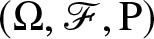 $(\Omega, \mathscr{F}, \mathrm{P})$ be a complete probability space with filtration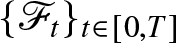 $\{\mathscr{F}_{t}\}_{t\in[0,T]}$, where $\mathscr{F}_{t}$ represents the information available in the market up to time $t$. We assume that the filtration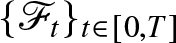 $\{\mathscr{F}_{t}\}_{t\in[0,T]}$ satisfies the usual conditions of completeness and right-continuity. We suppose that all stochastic processes and random variables are well-defined on this probability space and $\mathcal{G}$-adapted, where the filtration $\mathcal{G}$ is an enlarged filtration defined as $\mathcal{G}_{t}=\mathscr{F}_{t}\vee\mathscr{H}_{t}$. The filtration $\mathscr{F}_{t}$ is generated by the insurer’s reserve process $U(t)$ and the price process of a risky asset $S(t)$, while $\mathscr{H}_{t}$ is the filtration generated by the default process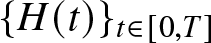 $\{H(t)\}_{t\in[0,T]}$, with $H(t)=I_{\{\tau\leq t\}}$, where $I$ is an indicator function and $\tau$ is the default time of a corporate bond. We also assume that $Q$ is a risk-neutral measure equivalent to the real-world measure $P$.
$P$.
2.1. Dynamics of financial market
We assume that the financial market consists of a risk-free asset, a risky asset, and a corporate zero-coupon bond that can default. The price processes are represented by 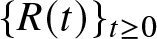 $\{R(t)\}_{t\geq0}$,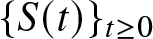 $\{S(t)\}_{t\geq0}$, and $\{p(t,T_1)\}_{t\geq0}$, where $T_1$ is a fixed time horizon. These processes are defined on a completely filtered probability space $(\Omega, \mathcal{G}, \mathrm{P})$. We assume the martingale invariance property: under the real-world probability measure $\mathrm{P}$, every square-integrable $\mathscr{F}_{t}$-martingale also remains a square-integrable $\mathcal{G}$-martingale.
The risk-free asset has a fixed continuously compounded return rate  $r\geq0$, and follows
 \begin{equation}
\mathrm{d}R(t)=rR(t)\mathrm{d}t.
\end{equation}
\begin{equation}
\mathrm{d}R(t)=rR(t)\mathrm{d}t.
\end{equation}Next, we assume that the risky asset in the market follows a constant volatility model:
 \begin{equation}
dS(t)=S(t)[(r+\alpha) dt+\beta dW_{1}(t)],~~S(0)=s\geq0,
\end{equation}
\begin{equation}
dS(t)=S(t)[(r+\alpha) dt+\beta dW_{1}(t)],~~S(0)=s\geq0,
\end{equation}where  $\alpha$ and $\beta$ are positive constants. $\alpha$ measures the performance of the risky asset compared to the risk-free asset and represents the amount of additional return the insurer receives for each unit of risk added. $\beta$ is the volatility of the risky asset and measures the magnitude of the asset’s risk.
Next, we follow Bielecki and Jang [Reference Bielecki and Jang5] and directly model the price process of a corporate zero-coupon bond under the real-world probability measure  $\mathrm{P}$. The bond is subject to default, and we assume that $T_{1}$ and $\tau$ are the maturity date of the corporate bond and the default time, respectively. Therefore, the default process is defined by a Poisson process $H(t)=1_{\{\tau\leq t\}}$ with constant intensity $h^{p}$ under the real-world measure $\mathrm{P}$. Following Bielecki and Jang [Reference Bielecki and Jang5], we can define
 \begin{equation*}dM^{p}(t)=H(t)-\int^{t}_{0}(1-H(s-))h^{p}ds,\end{equation*}
which is a  $\mathcal{G}$-martingale under $P$. In the event of default, the investor can recover a modest percentage of the pre-default market value of the defaultable bond. Let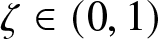 $\zeta \in (0,1)$ denote the constant loss rate of the corporate bond and $1-\zeta$ the default recovery rate. According to Lemma 2 in Bielecki and Jang [Reference Bielecki and Jang5], the arrival intensity of default under the risk-neutral measure $Q$ is given by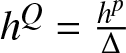 $h^{Q}=\frac{h^{p}}{\Delta}$, where $\frac{1}{\Delta}$ denotes the default risk premium. Consistent with Lemma 3 in Bielecki and Jang [Reference Bielecki and Jang5], the dynamics of the defaultable bond under the measure $P$ is given by:
 \begin{equation*}dp(t,T_{1})=p(t-,T_1)[rdt+(1-H(t-))\eta(1-\Delta)dt-(1-H(t-))\zeta dM^{p}(t)],\end{equation*}
where 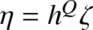 $\eta=h^{Q}\zeta$ is the risk-neutral credit spread.
2.2. Dynamics of the surplus process
Assuming that there are two competing insurance companies, whose surplus processes  $U_{k}(t), (k=1,2)$ can be described as follows:
 \begin{equation}
U_{k}(t)=u_{k}+d_{k}t-P_{k}(t),
\end{equation}
\begin{equation}
U_{k}(t)=u_{k}+d_{k}t-P_{k}(t),
\end{equation}where  $u_{k}$ is the initial surplus, $d_k$ is the fixed premium income rate of insurance company $k$ at time $t$,
$t$,  $P_{k}(t)$ represents the cumulative claims of the insurance business up to time $t$, and the aggregate claim processes for the two competing companies are given by:
 \begin{equation*}P_1(t)=\sum_{i=1}^{N_{1}(t)+N(t)}Y_{1i}~~~\mathrm{and}~~~P_2(t)=\sum_{i=1}^{N_{2}(t)+N(t)}Y_{2i}, \end{equation*}
where  $P_{1}(t)$ and $P_{2}(t)$ are two compound Poisson processes, $\{N(t), {t\geq0}\}$ and ${\{N_{k}(t), {t\geq0}\}}(k=1,2)$ are independent Poisson processes with intensities $\lambda$ and $\lambda_{k}, {k=1,2}$, respectively. The claim sizes of the first (second) insurance company, $\{Y_{ki},\}$, are assumed to be independent and identically distributed (i.i.d.) positive random variables, following a common distribution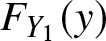 $F_{Y_1}(y)$ (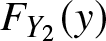 $F_{Y_2}(y)$) with first moments $\mu_k$ and second moments $\sigma_k$. These claim sizes are independent of $N(t)$ and $N_{k}(t)$ ( $k=1,2$). For each insurance company, we assume that the premium income rate $d_k$ is calculated according to the expected value principle, i.e., $d_k=(1+\eta_{k})(\lambda+\lambda_{k})\mu_k$, where $\eta_k$ is the non-negative safety loading of insurer $k$.
$k$.
Furthermore, we now consider that each insurance company can transfer part of the claim risk by continuously paying premiums to purchase proportional reinsurance in order to protect against this risk. The reinsurer’s premium is computed according to the variance premium principle. The corresponding reserve process for insurer  $k$ is then given by:
 \begin{equation}
dU_k(t)=(d_k-\delta_{k}(q_{k}(t)))dt-q_{k}(t)dP_{k}(t),
\end{equation}
\begin{equation}
dU_k(t)=(d_k-\delta_{k}(q_{k}(t)))dt-q_{k}(t)dP_{k}(t),
\end{equation}where  $q_k(t)$ is the proportion of claim risk undertaken by insurer $k$, while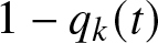 $1-q_k(t)$ is the proportion of claim risk undertaken by the reinsurer. The term $\delta_k(t)=(\lambda_k+\lambda)(1-q_k(t))\mu_k+\theta_k(1-q_{k}(t))^{2}(\lambda_k+\lambda)\sigma^{2}_{k}$ represents the reinsurer’s premium, with a safety loading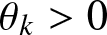 $\theta_k \gt 0$. Next, we use the Poisson random measures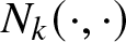 $N_{k}(\cdot,\cdot)$ and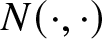 $N(\cdot,\cdot)$ on $\Omega\times[0,T]\times[0,\infty)$ to represent the compound Poisson process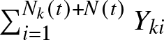 $\sum_{i=1}^{N_{k}(t)+N(t)}Y_{ki}$ as
 \begin{equation*}\sum^{N_{k}(t)+N(t)}_{i=1}Y_{ki}=\int^{t}_{0}\int^{\infty}_{0}q_{k}(s)y_{k}N_{k}(ds,dy_{k})+\int^{t}_{0}\int^{\infty}_{0}q_{k}(s)y_{k}N(ds,dy_{k}),~~~\forall t\in[0,T],~~k=1~or~2.\end{equation*}
 We denote by  $v_{k}(dt,dy_{k})=\lambda_{k}dtF_{Y_k}(dy_{k})$ and $v(dt,dy_{k})=\lambda dtF_{Y_k}(dy_{k})$ the compensators of the Poisson random measures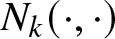 $N_{k}(\cdot,\cdot)$ and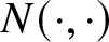 $N(\cdot,\cdot)$, respectively. Thus, we obtain
 \begin{equation*}E\bigg{[}\sum^{N_{k}(t)+N(t)}_{i=1}Y_{ki}\bigg{]}=\int^{t}_{0}\int^{\infty}_{0}y_{k}v_{k}(ds,dy_{k})+\int^{t}_{0}\int^{\infty}_{0}y_{k}v(ds,dy_{k}).\end{equation*}
 We define 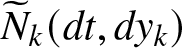 $\widetilde{N}_{k}(dt,dy_k)$ and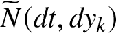 $\widetilde{N}(dt,dy_k)$ as the compensated Poisson random measures of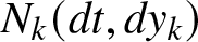 $N_{k}(dt,dy_k)$ and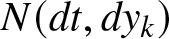 $N(dt,dy_k)$, respectively.
2.3. Wealth process with bounded memory
In this model, we assume that the two competing insurers can purchase risk-free assets, risky assets, and defaultable corporate zero-coupon bonds in the financial markets. Additionally, they can purchase proportional reinsurance, thereby increasing their returns and managing their risk exposure through investment and reinsurance. The investment horizon is [0, T] with 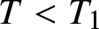 $T \lt T_{1}$. Thus, the wealth process of insurer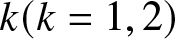 $k(k=1,2)$ follows:
 \begin{equation}
\begin{aligned}
dX^{\pi_k}_{k}(t)&=\frac{X^{\pi_k}_{k}(t-)-{\omega_{k}(t)}-\xi_{k}(t)}{R(t)}dR(t)+\frac{\xi_{k}(t)}{S(t)}dS(t)+\frac{\omega_{k}(t)}{p(t-,T_{1})}dp(t,T_{1})+dU_k(t)\\
&=[rX^{\pi_k}_{k}(t-)+d_{k}-(\lambda_k+\lambda)(1-q_k(t))\mu_k-\theta_k(1-q_{k}(t))^{2}(\lambda_k+\lambda)\sigma^{2}_{k}+\xi_{k}(t)\alpha \\
&+\omega_{k}(t)(1-H(t-))\eta(1-\Delta)]dt-\omega_{k}(t)(1-H(t-))\zeta dM^{p}(t)\\
&+\xi_{k}(t)\beta dW_{1}(t)-\int^{\infty}_{0}q_{k}(t)y_{k}N_{k}(dt,dy_{k})-\int^{\infty}_{0}q_{k}(t)y_{k}N(dt,dy_{k}),
\end{aligned}
\end{equation}
\begin{equation}
\begin{aligned}
dX^{\pi_k}_{k}(t)&=\frac{X^{\pi_k}_{k}(t-)-{\omega_{k}(t)}-\xi_{k}(t)}{R(t)}dR(t)+\frac{\xi_{k}(t)}{S(t)}dS(t)+\frac{\omega_{k}(t)}{p(t-,T_{1})}dp(t,T_{1})+dU_k(t)\\
&=[rX^{\pi_k}_{k}(t-)+d_{k}-(\lambda_k+\lambda)(1-q_k(t))\mu_k-\theta_k(1-q_{k}(t))^{2}(\lambda_k+\lambda)\sigma^{2}_{k}+\xi_{k}(t)\alpha \\
&+\omega_{k}(t)(1-H(t-))\eta(1-\Delta)]dt-\omega_{k}(t)(1-H(t-))\zeta dM^{p}(t)\\
&+\xi_{k}(t)\beta dW_{1}(t)-\int^{\infty}_{0}q_{k}(t)y_{k}N_{k}(dt,dy_{k})-\int^{\infty}_{0}q_{k}(t)y_{k}N(dt,dy_{k}),
\end{aligned}
\end{equation}where  $\xi_{k}(t)$ is the amount of insurer $k$’s wealth invested in stock and $\omega_{k}(t)$ is the amount of insurer $k$’s wealth invested in the corporate bond. Then, the capital invested in the risk-free asset is $X^{\pi_k}_{k}(t)-\xi_{k}(t)-\omega_{k}(t)$. Denote the reinsurance-investment control policy of insurer $k$ at time $t$ by $\pi_{k}(t)=(q_{k}(t)$, $\xi_{k}(t)$, $\omega_{k}(t))$, for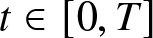 $t\in[0,T]$. Due to the property of bounded memory, the insurer’s strategy depends instantaneously on the exogenous capital inflow or outflow of current wealth. For example, if the insurer’s recent past wealth is in a profitable position, a portion of the surplus wealth can be taken out by the insurer and distributed to shareholders as dividends, resulting in an outflow of wealth. Conversely, if an inflow of funds is necessary for the normal operation of the insurance company due to mismanagement of the company’s capital or a downturn in the financial markets, this results in an inflow of funds. Similar to Bai et al. [Reference Bai, Zhou, Xiao, Gao and Zhong2], we define two new processes as follows:
 \begin{eqnarray*}
\begin{aligned}
&Y^{\pi_{k}}_{k}(t)\triangleq \int^{0}_{-u_{k}}e^{\overline{\alpha_{k}} s}X^{\pi_k}_{k}(t+s-)ds,\\
&Z^{\pi_{k}}_{k}(t)\triangleq X^{\pi_k}_{k}(t-u_{k}),~~\forall t\in[0,T],~~k\in\{1,2\}.
\end{aligned}
\end{eqnarray*}
\begin{eqnarray*}
\begin{aligned}
&Y^{\pi_{k}}_{k}(t)\triangleq \int^{0}_{-u_{k}}e^{\overline{\alpha_{k}} s}X^{\pi_k}_{k}(t+s-)ds,\\
&Z^{\pi_{k}}_{k}(t)\triangleq X^{\pi_k}_{k}(t-u_{k}),~~\forall t\in[0,T],~~k\in\{1,2\}.
\end{aligned}
\end{eqnarray*} Let 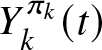 $Y^{\pi_{k}}_{k}(t)$ and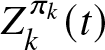 $Z^{\pi_{k}}_{k}(t)$ represent the integrated and pointwise delayed information of insurer $k$’s wealth process in the past horizon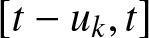 $[t-u_k,t]$, respectively, where $u_{k}$ is a delay parameter of insurer $k$ and $\overline{\alpha_{k}}$ is weight coefficient of insurer $k$.
$k$.
Let  $f_{k}(t,X^{\pi_k}_{k}(t)-Y^{\pi_{k}}_{k}(t),X^{\pi_k}_{k}(t)-Z^{\pi_{k}}_{k}(t))$ represent the exogenous capital inflow $/$outflow of insurer $k$ at time $t$, where $X^{\pi_k}_{k}(t)-Y^{\pi_{k}}_{k}(t)$ is the average performance and $X^{\pi_k}_{k}(t)-Z^{\pi_{k}}_{k}(t)$ is the absolute performance during the period $[t-u_{k},t]$. Similar to studies by Shen and Zeng [Reference Shen and Zeng28], Deng et al. [Reference Deng, Bian and Wu12] and Bai et al. [Reference Bai, Zhou, Xiao, Gao and Zhong2] when there is capital inflow $/$outflow, the wealth process of insurer $k$ becomes
 \begin{equation}
\begin{aligned}
dX^{\pi_k}_{k}(t)=\, &\frac{X^{\pi_k}_{k}(t-)-\upsilon_{k}(t)-\xi_{k}(t)}{R(t)}dR(t)+\frac{\xi_{k}(t)}{S(t)}dS(t)+\frac{\omega_{k}(t)}{p(t-,T_{1})}dp(t,T_{1})+dU_k(t)\\
&-f_{k}(t,X^{\pi_k}_{k}(t-)-Y^{\pi_{k}}_{k}(t-),X^{\pi_k}_{k}(t-)-Z^{\pi_{k}}_{k}(t-))dt.\\
\end{aligned}
\end{equation}
\begin{equation}
\begin{aligned}
dX^{\pi_k}_{k}(t)=\, &\frac{X^{\pi_k}_{k}(t-)-\upsilon_{k}(t)-\xi_{k}(t)}{R(t)}dR(t)+\frac{\xi_{k}(t)}{S(t)}dS(t)+\frac{\omega_{k}(t)}{p(t-,T_{1})}dp(t,T_{1})+dU_k(t)\\
&-f_{k}(t,X^{\pi_k}_{k}(t-)-Y^{\pi_{k}}_{k}(t-),X^{\pi_k}_{k}(t-)-Z^{\pi_{k}}_{k}(t-))dt.\\
\end{aligned}
\end{equation} When the company has been well-run for a period of time, it will naturally have larger returns. The insurance company will then distribute a portion of these returns to its shareholders as dividends. This corresponds to the situation where  $f_{k}(t,X^{\pi_k}_{k}(t)-Y^{\pi_{k}}_{k}(t),X^{\pi_k}_{k}(t)-Z^{\pi_{k}}_{k}(t)) \gt 0$, i.e., $X^{\pi_k}_{k}(t) \gt Y^{\pi_{k}}_{k}(t)$ and $X^{\pi_k}_{k}(t) \gt Z^{\pi_{k}}_{k}(t)$. Conversely, if the insurer has performed poorly over time, it will need to make a capital injection or raise capital to cover the corresponding losses. This corresponds to an inflow of capital, where $f_{k}(t,X^{\pi_k}_{k}(t)-Y^{\pi_{k}}_{k}(t),X^{\pi_k}_{k}(t)-Z^{\pi_{k}}_{k}(t)) \lt 0$, i.e., $X^{\pi_k}_{k}(t) \lt Y^{\pi_{k}}_{k}(t)$ and $X^{\pi_k}_{k}(t) \lt Z^{\pi_{k}}_{k}(t)$. Similar to Bai et al. [Reference Bai, Zhou, Xiao, Gao and Zhong2], we assume
 \begin{equation}
f_{k}(t,X^{\pi_k}_{k}(t)-Y^{\pi_{k}}_{k}(t),X^{\pi_k}_{k}(t)-Z^{\pi_{k}}_{k}(t))=B_{k}(X^{\pi_k}_{k}(t)-Y^{\pi_{k}}_{k}(t))+C_{k}(X^{\pi_k}_{k}(t)-Z^{\pi_{k}}_{k}(t)),
\end{equation}
\begin{equation}
f_{k}(t,X^{\pi_k}_{k}(t)-Y^{\pi_{k}}_{k}(t),X^{\pi_k}_{k}(t)-Z^{\pi_{k}}_{k}(t))=B_{k}(X^{\pi_k}_{k}(t)-Y^{\pi_{k}}_{k}(t))+C_{k}(X^{\pi_k}_{k}(t)-Z^{\pi_{k}}_{k}(t)),
\end{equation}where  $B_{k}$ and $C_{k}$ are two non-negative constants. In practice, the amount of capital inflows/outflows is a linearly weighted sum of average and absolute performance. To distinguish insurer 1 from insurer 2, we assume that the delay parameters of the two insurers are not equal, i.e., $\overline{\alpha_{1}}\neq \overline{\alpha_{2}}$,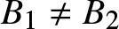 $B_{1}\neq B_{2}$ and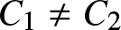 $C_{1}\neq C_{2}$. Combining Eq. (2.5), (2.6), and (2.7), the wealth processes of insurer $k$ are defined by the following stochastic differential delay equation (SDDE).
 \begin{equation}
\begin{aligned}
dX^{\pi_k}_{k}(t)=
&[A_{k}X^{\pi_k}_{k}(t-)+d_{k}-(\lambda_k+\lambda)(1-q_k(t))\mu_k-\theta_k(1-q_{k}(t))^{2}(\lambda_k+\lambda)\sigma^{2}_{k}+\xi_{k}(t)\alpha\\
&+\omega_{k}(t)(1-H(t-))\eta(1-\Delta)+B_{k}Y^{\pi_{k}}_{k}(t)+C_{k}Z^{\pi_{k}}_{k}(t)]dt\\
&+\xi_{k}(t)\beta dW_{1}(t)-\omega_{k}(t)(1-H(t-))\zeta dM^{p}(t)\\
&-\int^{\infty}_{0}q_{k}(t)y_{k}N_{k}(dt,dy_{k})-\int^{\infty}_{0}q_{k}(t)y_{k}N(dt,dy_{k}),\\
\end{aligned}
\end{equation}
\begin{equation}
\begin{aligned}
dX^{\pi_k}_{k}(t)=
&[A_{k}X^{\pi_k}_{k}(t-)+d_{k}-(\lambda_k+\lambda)(1-q_k(t))\mu_k-\theta_k(1-q_{k}(t))^{2}(\lambda_k+\lambda)\sigma^{2}_{k}+\xi_{k}(t)\alpha\\
&+\omega_{k}(t)(1-H(t-))\eta(1-\Delta)+B_{k}Y^{\pi_{k}}_{k}(t)+C_{k}Z^{\pi_{k}}_{k}(t)]dt\\
&+\xi_{k}(t)\beta dW_{1}(t)-\omega_{k}(t)(1-H(t-))\zeta dM^{p}(t)\\
&-\int^{\infty}_{0}q_{k}(t)y_{k}N_{k}(dt,dy_{k})-\int^{\infty}_{0}q_{k}(t)y_{k}N(dt,dy_{k}),\\
\end{aligned}
\end{equation}where  $A_{k}=r-B_{k}-C_{k}$. To simplify the solution procedure, we assume that $X^{\pi_k}_{k}(t)=x_{k}$ for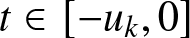 $t\in[-u_{k},0]$, i.e., insurer $k$ has not made any transactions from time $-u_{k}$ to time zero. Consequently, there is no change in insurer $k$’s wealth during this period, and the initial value of the insurer’s average performance is $Y^{\pi_{k}}_{k}(0)=\frac{x_{k}(1-e^{-\overline{\alpha_{k}}u_{k}})}{\overline{\alpha_{k}}}$.
In most of the literature on optimal reinsurance-investment control problems, the true probability distribution of insurance surplus and assets in the financial market is assumed to be known by insurers. However, there are many factors in insurance and financial risk of which insurers are unaware but that may significantly affect the estimation of model parameters. This uncertainty due to lack of information is known as ambiguity. In this paper, we assume that insurers are not only risk-averse but also ambiguity-averse. Most of the literature has investigated the general robust utility function of the form
 \begin{equation}
\inf_{Q\in\mathcal{Q}}E^{Q}[U(X)+h_{\beta}(Q)],
\end{equation}
\begin{equation}
\inf_{Q\in\mathcal{Q}}E^{Q}[U(X)+h_{\beta}(Q)],
\end{equation}where  $X$ is a random payoff, $\mathcal{Q}$ is the set of probability measures such that each $Q$ is equivalent to $P$,
$P$,  $U$ is a utility function, and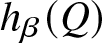 $h_{\beta}(Q)$ is a penalty function that measures the difference between $Q$ and $P$. Nevertheless, a limitation of the robust utility (2.9) is that it only accepts attitudes that are extremely ambiguity-averse. Few behavioral experiments support such extreme pessimistic ambiguity on the part of policymakers. Therefore, Li et al. [Reference Li, Li and Xiong19] proposed a new mean-variance criterion inspired by robust utility (2.9) and $alpha$-maximin expected utility, called the $alpha$-maximin mean-variance criterion, given by
 \begin{equation}
alpha\inf_{Q\in\mathcal{Q}}\{E^{Q}[X]+\gamma Var^{Q}[X]+E^{Q}[h_{\beta}(Q)]\}+(1-alpha)\sup_{Q\in\mathcal{Q}}\{E^{Q}[X]+\gamma Var^{Q}[X]-E^{Q}[h_{\beta}(Q)]\},
\end{equation}
\begin{equation}
alpha\inf_{Q\in\mathcal{Q}}\{E^{Q}[X]+\gamma Var^{Q}[X]+E^{Q}[h_{\beta}(Q)]\}+(1-alpha)\sup_{Q\in\mathcal{Q}}\{E^{Q}[X]+\gamma Var^{Q}[X]-E^{Q}[h_{\beta}(Q)]\},
\end{equation}where  $alpha$ designates the magnitude of ambiguity aversion, with $alpha$ equal to 1, 1/2, and 0 representing extreme ambiguity aversion, neutral ambiguity, and extreme ambiguity pursuit, respectively. In this paper, we investigate $alpha$-robust control strategies instead of the general robust problems under a non-zero sum differential game, because the $alpha$-maximin mean-variance criterion allows insurers to have different levels of ambiguity aversion. To incorporate the ambiguity of insurance and financial risk, we define a set of probability measures $\mathcal{Q}=\{\mathrm{Q}|\mathrm{Q}\sim \mathrm{P}\}$, where $P$ is the reference probability measure and $Q$ is an equivalent probability measure of $P$, known as the alternative probability measure. First, we introduce the probability distortion function
 \begin{equation*}\phi_{k}=(\phi_{k1}(t),\phi_{k2}(t),\phi_{k3}(t,y_{k}),\phi_{k4}(t,y_{k}))_{t\in[0,T],y_{k} \gt 0}\in\Phi_{k},\end{equation*}
where we call  $\phi_{k}$ the density generator of insurer $k$. Here, $\phi_{k}$ is a measurable real-value process, and $\phi_{k1}(t)$, $\phi_{k2}(t)$, $\phi_{k3}(t,y_{k})$, and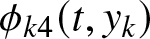 $\phi_{k4}(t,y_{k})$ are deterministic functions of $t$ and $y_{k}$, and satisfy
 \begin{eqnarray*}
\begin{aligned}
\exp&\bigg{\{}\int^{T}_{t}\frac{\phi_{k1}^{2}(s)}{2}+h^{p}\int^{t}_{0}(1-\phi_{k2}(s))(1-H(s))ds\\
&+\int^{T}_{t}\int^{\infty}_{0}[(1-\phi_{k3}(s,y_{k}))\ln(1-\phi_{k3}(s,y_{k}))+\phi_{k3}(s,y_{k})]\upsilon_{k}(dy_{k})ds\\
&+\int^{T}_{t}\int^{\infty}_{0}[(1-\phi_{k4}(s,y_{k}))\ln(1-\phi_{k4}(s,y_{k}))+\phi_{k4}(s,y_{k})]\upsilon(dy_{k})ds\bigg{\}} \lt \infty,
\end{aligned}
\end{eqnarray*}
\begin{eqnarray*}
\begin{aligned}
\exp&\bigg{\{}\int^{T}_{t}\frac{\phi_{k1}^{2}(s)}{2}+h^{p}\int^{t}_{0}(1-\phi_{k2}(s))(1-H(s))ds\\
&+\int^{T}_{t}\int^{\infty}_{0}[(1-\phi_{k3}(s,y_{k}))\ln(1-\phi_{k3}(s,y_{k}))+\phi_{k3}(s,y_{k})]\upsilon_{k}(dy_{k})ds\\
&+\int^{T}_{t}\int^{\infty}_{0}[(1-\phi_{k4}(s,y_{k}))\ln(1-\phi_{k4}(s,y_{k}))+\phi_{k4}(s,y_{k})]\upsilon(dy_{k})ds\bigg{\}} \lt \infty,
\end{aligned}
\end{eqnarray*}for any 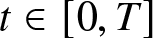 $t\in[0,T]$ (according to Li et al. [Reference Li, Li and Xiong19]). Furthermore, we define an exponential process $\{\Lambda^{\phi_{k}}(t)\}_{t\in[0,T]}$ by
 \begin{equation}
\begin{aligned}
\Lambda^{\phi_{k}}(t)&=\exp\bigg{\{}\!\int^{t}_{0}\phi_{k1}(s)ds-\frac{1}{2}\!\int^{t}_{0}\phi^{2}_{k1}(s)ds+\!\int^{t}_{0}\ln(\phi_{k2}(s))dH(s)+h^{p}\int^{t}_{0}\!(1-\phi_{k2}(s))(1-H(s))ds\\
&+\int^{t}_{0}\int^{\infty}_{0}\ln(1-\phi_{k3}(s,y_k))dN_{k}(ds,dy_k)+\int^{t}_{0}\int^{\infty}_{0}\phi_{k3}(s,y_{k}))\upsilon_{k}(dy_{k})ds\\
&+\int^{t}_{0}\int^{\infty}_{0}\ln(1-\phi_{k4}(s,y_k))dN(ds,dy_k)+\int^{t}_{0}\int^{\infty}_{0}\phi_{k4}(s,y_{k}))\upsilon(dy_{k})ds\bigg{\}}.
\end{aligned}
\end{equation}
\begin{equation}
\begin{aligned}
\Lambda^{\phi_{k}}(t)&=\exp\bigg{\{}\!\int^{t}_{0}\phi_{k1}(s)ds-\frac{1}{2}\!\int^{t}_{0}\phi^{2}_{k1}(s)ds+\!\int^{t}_{0}\ln(\phi_{k2}(s))dH(s)+h^{p}\int^{t}_{0}\!(1-\phi_{k2}(s))(1-H(s))ds\\
&+\int^{t}_{0}\int^{\infty}_{0}\ln(1-\phi_{k3}(s,y_k))dN_{k}(ds,dy_k)+\int^{t}_{0}\int^{\infty}_{0}\phi_{k3}(s,y_{k}))\upsilon_{k}(dy_{k})ds\\
&+\int^{t}_{0}\int^{\infty}_{0}\ln(1-\phi_{k4}(s,y_k))dN(ds,dy_k)+\int^{t}_{0}\int^{\infty}_{0}\phi_{k4}(s,y_{k}))\upsilon(dy_{k})ds\bigg{\}}.
\end{aligned}
\end{equation} By Girsanov’s theorem, for 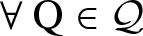 $\forall~\mathrm{Q}\in\mathcal{Q}$, there exists a process $\phi_{k}=(\phi_{k1}(t),\phi_{k2}(t),\phi_{k3}(t,y_{k}),\phi_{k4}(t,y_{k}))$ such that
 \begin{equation*}\frac{\mathrm{dQ}}{\mathrm{dP}}\bigg{|}_{\mathscr{F}_{t}}=\Lambda^{\phi_{k}}(t),\end{equation*}
where 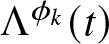 $\Lambda^{\phi_{k}}(t)$ is a $\mathrm{P}$-exponential martingale and satisfies $E[\Lambda^{\phi_{k}}(t)]=1$. Under the probability measure $Q$, we obtain
 \begin{equation*}dW^{Q^{\phi}}_{1}(t)=dW_{1}(t)-\phi_{k1}(t)dt,\end{equation*}
which is a  $Q$-Brownian motion, and $\widetilde{N}^{Q}_{k}(dt,dy_k)$ and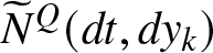 $\widetilde{N}^{Q}(dt,dy_k)$ satisfying
 \begin{equation*}\widetilde{N}^{Q}_{k}(dt,dy_k)=\widetilde{N}_{k}(dt,dy_k)+\phi_{k3}(t,y_{k})\upsilon_{k}(dy_{k})dt~\mathrm{and}~\widetilde{N}^{Q}(dt,dy_k)=\widetilde{N}(dt,dy_k)+\phi_{k4}(t,y_{k})\upsilon(dy_{k})dt,\end{equation*}
which are  $Q$-compensated Poisson random measures with compensators $(1-\phi_{k3}(t,y_k))\upsilon_{k}(dy_{k})$ and $(1-\phi_{k4}(t,y_k))\upsilon(dy_{k})$, respectively. Therefore, the SDDE of insurer $k$’s wealth process under the probability measure $Q$ is given by
 \begin{equation}
\begin{aligned}
dX^{\pi_k}_{k}(t)=
&\bigg{[}A_{k}X^{\pi_k}_{k}(t-)+d_{k}-(\lambda_k+\lambda)\mu_k-\theta_k(1-q_{k}(t))^{2}(\lambda_k+\lambda)\sigma^{2}_{k}+\xi_{k}(t)\alpha\\
&+\omega_{k}(t)(1-H(t-))\eta(1-\Delta)+B_{k}Y^{\pi_{k}}_{k}(t)+C_{k}Z^{\pi_{k}}_{k}(t)+\phi_{k1}\xi_{k}(t)\beta\\
&+\int^{\infty}_{0}q_{k}(t)y_{k}\phi_{k3}(t,y_k)\upsilon_{k}(dy_k)+\int^{\infty}_{0}q_{k}(t)y_{k}\phi_{k4}(t,y_k)\upsilon(dy_k)\bigg{]}dt\\
&+\xi_{k}(t)\beta dW^{Q^{\phi}}_{1}(t)-\omega_{k}(t)(1-H(t-))\zeta dM^{p}(t)\\
&-\int^{\infty}_{0}q_{k}(t)y_{k}\widetilde{N}^{Q^{\phi}}_{k}(dt,dy_{k})-\int^{\infty}_{0}q_{k}(t)y_{k}\widetilde{N}^{Q^{\phi}}(dt,dy_{k}).\\
\end{aligned}
\end{equation}
\begin{equation}
\begin{aligned}
dX^{\pi_k}_{k}(t)=
&\bigg{[}A_{k}X^{\pi_k}_{k}(t-)+d_{k}-(\lambda_k+\lambda)\mu_k-\theta_k(1-q_{k}(t))^{2}(\lambda_k+\lambda)\sigma^{2}_{k}+\xi_{k}(t)\alpha\\
&+\omega_{k}(t)(1-H(t-))\eta(1-\Delta)+B_{k}Y^{\pi_{k}}_{k}(t)+C_{k}Z^{\pi_{k}}_{k}(t)+\phi_{k1}\xi_{k}(t)\beta\\
&+\int^{\infty}_{0}q_{k}(t)y_{k}\phi_{k3}(t,y_k)\upsilon_{k}(dy_k)+\int^{\infty}_{0}q_{k}(t)y_{k}\phi_{k4}(t,y_k)\upsilon(dy_k)\bigg{]}dt\\
&+\xi_{k}(t)\beta dW^{Q^{\phi}}_{1}(t)-\omega_{k}(t)(1-H(t-))\zeta dM^{p}(t)\\
&-\int^{\infty}_{0}q_{k}(t)y_{k}\widetilde{N}^{Q^{\phi}}_{k}(dt,dy_{k})-\int^{\infty}_{0}q_{k}(t)y_{k}\widetilde{N}^{Q^{\phi}}(dt,dy_{k}).\\
\end{aligned}
\end{equation} The traditional analysis of optimal reinsurance and investment has focused on the decisions of a single agent. However, as noted by Deng et al. [Reference Deng, Zeng and Zhu13] and Bai et al. [Reference Bai, Zhou, Xiao, Gao and Zhong2], financial institutions are concerned about their relative performance compared to industry peers. As a result, insurers not only aim to control risk by purchasing reinsurance coverage and profiting from investments in financial markets, but also to surpass their competitors in terms of terminal wealth. We define the relative performance process of insurer  $k$, for $k,l\in\{1,2\}$ and $k\neq l$, as follows:
 \begin{eqnarray*}
\begin{aligned}
\hat{X}^{\pi_{k},\pi_{l}}_{k}(t)&=(1-n_{k})X^{\pi_{k}}_{k}(t)+n_{k}(X^{\pi_{k}}_{k}(t)-X^{\pi_{l}}_{l}(t))\\
&=X^{\pi_{k}}_{k}(t)-n_{k}X^{\pi_{l}}_{l}(t),
\end{aligned}
\end{eqnarray*}
\begin{eqnarray*}
\begin{aligned}
\hat{X}^{\pi_{k},\pi_{l}}_{k}(t)&=(1-n_{k})X^{\pi_{k}}_{k}(t)+n_{k}(X^{\pi_{k}}_{k}(t)-X^{\pi_{l}}_{l}(t))\\
&=X^{\pi_{k}}_{k}(t)-n_{k}X^{\pi_{l}}_{l}(t),
\end{aligned}
\end{eqnarray*}where the constant  $n_{k}\in[0,1]$ measures the sensitivity of insurer $k$ to the performance of his competitor. A larger $n_{k}$ implies that insurer $k$ is more concerned about increasing his relative surplus, making the game more competitive. The dynamics of $\hat{X}^{\pi_{k},\pi_{l}}_{k}(t)$ under $Q^{\phi_{k}}$ (representing the probability measure under $\phi_{k}$) are described by the following SDDE:
 \begin{align}d\hat{X}^{\pi_{k},\pi_{l}}_{k}(t)= & \bigg{[}A_{k}X^{\pi_k}_{k}(t-)-n_kA_{l}X^{\pi_l}_{l}(t-)+B_{k}Y^{\pi_{k}}_{k}(t)-n_kB_{l}Y^{\pi_{l}}_{l}(t)+C_{k}Z^{\pi_{k}}_{k}(t)-n_kC_{l}Z^{\pi_{l}}_{l}(t)\nonumber\\
& +d_{k}-(\lambda_k+\lambda)\mu_k-\theta_k(1-q_{k}(t))^{2}(\lambda_k+\lambda)\sigma^{2}_{k}-n_kd_{l}+n_k(\lambda_l+\lambda)\mu_l\nonumber\\
& +n_k\theta_l(1-q_{l}(t))^{2}(\lambda_l+\lambda)\sigma^{2}_{l}+(\xi_{k}(t)-n_k\xi_l(t))\alpha\nonumber\\
& +(\omega_{k}(t)-n_k\omega_{l}(t))(1-H(t-))\eta(1-\Delta)+(\phi_{k1}\xi_{k}(t)-n_k\phi_{l1}\xi_{l}(t))\beta\nonumber\\
& +\int^{\infty}_{0}q_{k}(t)y_{k}\phi_{k3}(t,y_k)\upsilon_{k}(dy_k)+\int^{\infty}_{0}q_{k}(t)y_{k}\phi_{k4}(t,y_k)\upsilon(dy_k)\nonumber\\
& -n_k\int^{\infty}_{0}q_{l}(t)y_{l}\phi_{l3}(t,y_l)\upsilon_{l}(dy_l)-n_k\int^{\infty}_{0}q_{l}(t)y_{l}\phi_{l4}(t,y_l)\upsilon(dy_l)\bigg{]}dt\nonumber\\
& +(\xi_{k}(t)-n_k\xi_l(t))\beta dW^{Q^{\phi}}_{1}(t)-(\omega_{k}(t)-n_k\omega_{l}(t))(1-H(t-))\zeta dM^{p}(t)\nonumber\\
& -\int^{\infty}_{0}q_{k}(t)y_{k}\widetilde{N}^{Q^{\phi}}_{k}(dt,dy_{k})-\int^{\infty}_{0}q_{k}(t)y_{k}\widetilde{N}^{Q^{\phi}}(dt,dy_{k})\nonumber\\
& +n_k\int^{\infty}_{0}q_{l}(t)y_{l}\widetilde{N}^{Q^{\phi}}_{l}(dt,dy_{l})+n_k\int^{\infty}_{0}q_{l}(t)y_{l}\widetilde{N}^{Q^{\phi}}(dt,dy_{l}),\end{align}
\begin{align}d\hat{X}^{\pi_{k},\pi_{l}}_{k}(t)= & \bigg{[}A_{k}X^{\pi_k}_{k}(t-)-n_kA_{l}X^{\pi_l}_{l}(t-)+B_{k}Y^{\pi_{k}}_{k}(t)-n_kB_{l}Y^{\pi_{l}}_{l}(t)+C_{k}Z^{\pi_{k}}_{k}(t)-n_kC_{l}Z^{\pi_{l}}_{l}(t)\nonumber\\
& +d_{k}-(\lambda_k+\lambda)\mu_k-\theta_k(1-q_{k}(t))^{2}(\lambda_k+\lambda)\sigma^{2}_{k}-n_kd_{l}+n_k(\lambda_l+\lambda)\mu_l\nonumber\\
& +n_k\theta_l(1-q_{l}(t))^{2}(\lambda_l+\lambda)\sigma^{2}_{l}+(\xi_{k}(t)-n_k\xi_l(t))\alpha\nonumber\\
& +(\omega_{k}(t)-n_k\omega_{l}(t))(1-H(t-))\eta(1-\Delta)+(\phi_{k1}\xi_{k}(t)-n_k\phi_{l1}\xi_{l}(t))\beta\nonumber\\
& +\int^{\infty}_{0}q_{k}(t)y_{k}\phi_{k3}(t,y_k)\upsilon_{k}(dy_k)+\int^{\infty}_{0}q_{k}(t)y_{k}\phi_{k4}(t,y_k)\upsilon(dy_k)\nonumber\\
& -n_k\int^{\infty}_{0}q_{l}(t)y_{l}\phi_{l3}(t,y_l)\upsilon_{l}(dy_l)-n_k\int^{\infty}_{0}q_{l}(t)y_{l}\phi_{l4}(t,y_l)\upsilon(dy_l)\bigg{]}dt\nonumber\\
& +(\xi_{k}(t)-n_k\xi_l(t))\beta dW^{Q^{\phi}}_{1}(t)-(\omega_{k}(t)-n_k\omega_{l}(t))(1-H(t-))\zeta dM^{p}(t)\nonumber\\
& -\int^{\infty}_{0}q_{k}(t)y_{k}\widetilde{N}^{Q^{\phi}}_{k}(dt,dy_{k})-\int^{\infty}_{0}q_{k}(t)y_{k}\widetilde{N}^{Q^{\phi}}(dt,dy_{k})\nonumber\\
& +n_k\int^{\infty}_{0}q_{l}(t)y_{l}\widetilde{N}^{Q^{\phi}}_{l}(dt,dy_{l})+n_k\int^{\infty}_{0}q_{l}(t)y_{l}\widetilde{N}^{Q^{\phi}}(dt,dy_{l}),\end{align}where  $\hat{X}^{\pi_{k},\pi_{l}}_{k}(0)={X}^{\pi_{k}}_{k}(0)-n_k{X}^{\pi_{l}}_{l}(0)\triangleq\hat{x}_{k}$. According to Hurwitz’s $alpha$-pessimism rule and the $alpha$-maxmin expected utility, Li et al. [Reference Li, Li and Xiong19] defined the $alpha$-robust mean-variance criterion for a controlled wealth process $\hat{X}^{\pi_{k},\pi_{l}}_{k}$ as follows:
 \begin{equation}
\begin{aligned}
J^{\pi_k,\pi_l}_{k}(t,\hat{x}_{k},y_{k},y_{l},h)&=\alpha_{k}\inf_{\phi\in\Phi}\underline{J}^{\pi_k,\pi_l,\phi_k}_{k}(t,\hat{x}_{k},y_{k},y_{l},h)+\hat{\alpha}_{k}\sup_{\phi\in\Phi}\overline{J}^{\pi_k,\pi_l,\phi_k}_{k}(t,\hat{x}_{k},y_{k},y_{l},h)\\
&=\alpha_{k}\underline{J}^{\pi_k,\pi_l,\underline{\phi_k}}_{k}(t,\hat{x}_{k},y_{k},y_{l},h)+\hat{\alpha}_{k}\overline{J}^{\pi_k,\pi_l,\overline{\phi_k}}_{k}(t,\hat{x}_{k},y_{k},y_{l},h),
\end{aligned}
\end{equation}
\begin{equation}
\begin{aligned}
J^{\pi_k,\pi_l}_{k}(t,\hat{x}_{k},y_{k},y_{l},h)&=\alpha_{k}\inf_{\phi\in\Phi}\underline{J}^{\pi_k,\pi_l,\phi_k}_{k}(t,\hat{x}_{k},y_{k},y_{l},h)+\hat{\alpha}_{k}\sup_{\phi\in\Phi}\overline{J}^{\pi_k,\pi_l,\phi_k}_{k}(t,\hat{x}_{k},y_{k},y_{l},h)\\
&=\alpha_{k}\underline{J}^{\pi_k,\pi_l,\underline{\phi_k}}_{k}(t,\hat{x}_{k},y_{k},y_{l},h)+\hat{\alpha}_{k}\overline{J}^{\pi_k,\pi_l,\overline{\phi_k}}_{k}(t,\hat{x}_{k},y_{k},y_{l},h),
\end{aligned}
\end{equation}where  $\alpha_k+\hat{\alpha}_k=1(\alpha_k\in[0,1])$,
 \begin{equation}
\begin{aligned}
\underline{J}^{\pi_k,\pi_l,\phi_{k}}_{k}(t,\hat{x}_{k},y_{k},y_{l},h)&=E^{Q^{\phi}}_{t,\hat{x}_{k},l,y_{k},y_{l},h}[\hat{X}^{\pi_{k},\pi_{l}}_{k}(T)+\vartheta_{k}Y_{k}(T)-n_{k}\vartheta_lY_{l}(T)]\\
&-\frac{\gamma_k}{2}Var^{Q^{\phi}}_{t,\hat{x}_{k},y_{k},y_{l},h}[\hat{X}^{\pi_{k},\pi_{l}}_{k}(T)+\vartheta_{k}Y_{k}(T)-n_{k}\vartheta_lY_{l}(T)]\\
&+\int^{T}_{t}h_{\beta}(\phi_{k})ds,
\end{aligned}
\end{equation}
\begin{equation}
\begin{aligned}
\underline{J}^{\pi_k,\pi_l,\phi_{k}}_{k}(t,\hat{x}_{k},y_{k},y_{l},h)&=E^{Q^{\phi}}_{t,\hat{x}_{k},l,y_{k},y_{l},h}[\hat{X}^{\pi_{k},\pi_{l}}_{k}(T)+\vartheta_{k}Y_{k}(T)-n_{k}\vartheta_lY_{l}(T)]\\
&-\frac{\gamma_k}{2}Var^{Q^{\phi}}_{t,\hat{x}_{k},y_{k},y_{l},h}[\hat{X}^{\pi_{k},\pi_{l}}_{k}(T)+\vartheta_{k}Y_{k}(T)-n_{k}\vartheta_lY_{l}(T)]\\
&+\int^{T}_{t}h_{\beta}(\phi_{k})ds,
\end{aligned}
\end{equation}which represents the term of ambiguity seeking, and the last equation represents the term of ambiguity aversion.
 \begin{equation}
\begin{aligned}
\overline{J}^{\pi_k,\pi_l,\phi_{k}}_{k}(t,\hat{x}_{k},y_{k},y_{l},h)&=E^{Q^{\phi}}_{t,\hat{x}_{k},l,y_{k},y_{l},h}[\hat{X}^{\pi_{k},\pi_{l}}_{k}(T)+\vartheta_{k}Y_{k}(T)-n_{k}\vartheta_lY_{l}(T)]\\
&-\frac{\gamma_k}{2}Var^{Q^{\phi}}_{t,\hat{x}_{k},y_{k},y_{l},h}[\hat{X}^{\pi_{k},\pi_{l}}_{k}(T)+\vartheta_{k}Y_{k}(T)-n_{k}\vartheta_lY_{l}(T)]\\
&-\int^{T}_{t}h_{\beta}(\phi_{k})ds,
\end{aligned}
\end{equation}
\begin{equation}
\begin{aligned}
\overline{J}^{\pi_k,\pi_l,\phi_{k}}_{k}(t,\hat{x}_{k},y_{k},y_{l},h)&=E^{Q^{\phi}}_{t,\hat{x}_{k},l,y_{k},y_{l},h}[\hat{X}^{\pi_{k},\pi_{l}}_{k}(T)+\vartheta_{k}Y_{k}(T)-n_{k}\vartheta_lY_{l}(T)]\\
&-\frac{\gamma_k}{2}Var^{Q^{\phi}}_{t,\hat{x}_{k},y_{k},y_{l},h}[\hat{X}^{\pi_{k},\pi_{l}}_{k}(T)+\vartheta_{k}Y_{k}(T)-n_{k}\vartheta_lY_{l}(T)]\\
&-\int^{T}_{t}h_{\beta}(\phi_{k})ds,
\end{aligned}
\end{equation}where  $\underline{\phi}_{k}$ and $\overline{\phi}_{k}$ are the probability distortion functions achieving the infimum and supremum in (2.14), and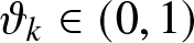 $\vartheta_k\in (0,1)$ ( $\vartheta_l$) values the weight of $Y_k(T)$( $Y_l(T)$) and measures the sensitivity of insurer $k$ to the performance of insurer $k$(
$k$( $l$). Although there might exist uncertainty or errors in the parameters of the reference model, the reference measure $P$ is the best description of the real model based on the information obtained so far. Thus, ambiguity-averse insurers or ambiguity seekers aim to consider alternative models that do not deviate too far from the reference model. The alternative measures and the penalization term in (2.15) and (2.16) illustrate the trade-off between not completely relying on the reference model and not deviating too far from it. The penalty function is selected to
 \begin{equation}
\begin{aligned}
h_{\beta}(\phi_k(t))&=\frac{\phi_{k1}(t)^{2}}{2\beta_{k1}}+\frac{(\phi_{k2}(t)\ln\phi_{k2}(t)-\phi_{k2}(t)+1)h^{p}(1-H(t-))}{\beta_{k2}}\\
&+\frac{\int^{\infty}_{0}[(1-\phi_{k3}(t,y_k))\ln(1-\phi_{k3}(t,y_k))+\phi_{k3}(t,y_k)]\upsilon_{k}(dy_{k})}{\beta_{k3}}\\
&+\frac{\int^{\infty}_{0}[(1-\phi_{k4}(t,y_k))\ln(1-\phi_{k4}(t,y_k))+\phi_{k4}(t,y_k)]\upsilon(dy_{k})}{\beta_{k4}}.
\end{aligned}
\end{equation}
\begin{equation}
\begin{aligned}
h_{\beta}(\phi_k(t))&=\frac{\phi_{k1}(t)^{2}}{2\beta_{k1}}+\frac{(\phi_{k2}(t)\ln\phi_{k2}(t)-\phi_{k2}(t)+1)h^{p}(1-H(t-))}{\beta_{k2}}\\
&+\frac{\int^{\infty}_{0}[(1-\phi_{k3}(t,y_k))\ln(1-\phi_{k3}(t,y_k))+\phi_{k3}(t,y_k)]\upsilon_{k}(dy_{k})}{\beta_{k3}}\\
&+\frac{\int^{\infty}_{0}[(1-\phi_{k4}(t,y_k))\ln(1-\phi_{k4}(t,y_k))+\phi_{k4}(t,y_k)]\upsilon(dy_{k})}{\beta_{k4}}.
\end{aligned}
\end{equation} Hence, the deviation of the alternative measure  ${Q}^{\phi}$ from the reference measure $P$ for insurer $k$ is penalized by the relative entropy $\int^{T}_{t}h_{\beta}(\phi_k(s))ds$. The constant vector $\beta_{k}=(\beta_{k1},~\beta_{k2},~\beta_{k3},~\beta_{k4})\in(0,\infty)^{4}$ represents the ambiguity parameters. These parameters determine the magnitude of the penalization for deviating from the reference measure $P$. Specifically, the term $1/\beta_{ki}$ acts as the weight of the penalty term. Consequently, as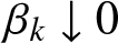 $\beta_{k}\downarrow0$, the penalty tends to infinity, implying that the insurer has full confidence in the reference model and does not consider alternative measures (i.e.,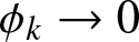 $\phi_{k} \to 0$). Conversely, as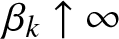 $\beta_{k}\uparrow\infty$, the penalty vanishes, indicating that the insurer has little confidence in the reference model and considers the environment to be extremely ambiguous.
Definition 2.1. A reinsurance-investment control strategy  $\pi_{k}(t)=(q_{k}(t),\xi_{k}(t),\omega_{k}(t))$ is called an admissible strategy if it satisfies the following conditions:
(1) $q_{k}(t),\xi_{k}(t)$, and
$\omega_{k}(t)\in[0,\infty]$,
$\forall t\in[0,T]$;
$q_{k}(t),\xi_{k}(t)$, and
$\omega_{k}(t)\in[0,\infty]$,
$\forall t\in[0,T]$;(2)
$\pi_{k}(t)$ is
$\mathcal{G}$-progressively measurable;(3)
$E^{Q^{\underline{\phi}_{k}}}[\int^{T}_{t}||\pi_{k}(s)||^{2}ds] \lt \infty$ and
$E^{Q^{\overline{\phi}_{k}}}[\int^{T}_{t}||\pi_{k}(s)||^{2}ds] \lt \infty$, where
$||\pi_{k}(s)||^{2}=q^{2}_{k}(s)+\xi^{2}_{k}(t)+\omega^{2}_{k}(s)$,
$Q^{\underline{\phi}_{k}}$ and
$Q^{\overline{\phi}_{k}}$ are the chosen probability measures to describe the worse-case scenario and will be determined later;(4) The stochastic differential equation (2.8) has a pathwise unique solution
$X^{\pi_{k}}_{k}(t,x_k,y_k,y_{l},h)$.


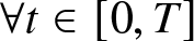







Let  $\Pi_{k}$ denote the set of all admissible strategies of insurer $k$.
$k$.
3. Formulation of a non-zero-sum game
Both insurers choose an admissible reinsurance and investment strategy  $\pi_{k}$ to maximize the expected terminal surplus relative to that of their competitor and minimize the variance of this relative terminal surplus under the $\alpha$-robust criterion. Unlike the max-min approach, which considers only the worst-case scenario, the $\alpha$-robust criterion adopted here involves a convex combination of the worst-case and best-case scenarios regarding the alternative measures. Each insurer cares about the difference between its terminal wealth and that of the other, and strives to perform better relative to its competitor. Under this optimization criterion, we can formulate the strategic interaction between the two insurers as follows:
Problem 1. The robust non-zero-sum stochastic differential game between two competing ambiguity-averse insurers under the mean-variance criterion is to find a Nash equilibrium  $(\pi_{1}, \pi_{2})\in\Pi_{1}\times\Pi_{2}$ such that the objective of insurer 1 satisfies
 \begin{equation*}\inf_{\phi_{1}\in\Phi_{1}}\underline{J}^{\pi^{*}_1,\pi^{*}_2,\phi_{1}}_{1}(t,\hat{x}_{1},y_{1},y_{2},h)\geq \inf_{\phi_{1}\in\Phi_{1}}\underline{J}^{\pi_1,\pi^{*}_2,\phi_{1}}_{1}(t,\hat{x}_{1},y_{1},y_{2},h),\end{equation*}
and
 \begin{equation*}\sup_{\phi_{1}\in\Phi_{1}}\overline{J}^{\pi^{*}_1,\pi^{*}_2,\phi_{1}}_{1}(t,\hat{x}_{1},y_{1},y_{2},h)\geq \sup_{\phi_{1}\in\Phi_{1}}\overline{J}^{\pi_1,\pi^{*}_2,\phi_{1}}_{1}(t,\hat{x}_{1},y_{1},y_{2},h).\end{equation*}
The objective of insurer 2 satisfies
 \begin{equation*}\inf_{\phi_{2}\in\Phi_{2}}\underline{J}^{\pi^{*}_1,\pi^{*}_2,\phi_{1}}_{2}(t,\hat{x}_{2},y_{1},y_{2},h)\geq \inf_{\phi_{2}\in\Phi_{2}}\underline{J}^{\pi^{*}_1,\pi_2,\phi_{1}}_{2}(t,\hat{x}_{2},y_{1},y_{2},h),\end{equation*}
and
 \begin{equation*}\sup_{\phi_{2}\in\Phi_{2}}\overline{J}^{\pi^{*}_1,\pi^{*}_2,\phi_{1}}_{2}(t,\hat{x}_{2},y_{1},y_{2},h)\geq \sup_{\phi_{2}\in\Phi_{2}}\overline{J}^{\pi^{*}_1,\pi_2,\phi_{1}}_{2}(t,\hat{x}_{2},y_{1},y_{2},h).\end{equation*}
 The main objective of insurer  $k$ is to investigate the $alpha$-robust, time-consistent reinsurance-investment problem as follows:
 \begin{equation}
\begin{aligned}
V_{k}(t,\hat{x}_{k},y_{k},y_{l},h)&=\sup_{\pi_{k}\in\Pi_{k}}J^{\pi_k,\pi^{*}_l}_{k}(t,\hat{x}_{k},y_{k},y_{l},h)\\
&=\sup_{\pi_{k}\in\Pi_{k}}\{\alpha_k\inf_{\phi\in\Phi}\underline{J}^{\pi_k,\pi^{*}_l,\phi_k}_{k}(t,\hat{x}_{k},y_{k},y_{l},h)+\hat{\alpha}_k\sup_{\phi_k\in\Phi_k}\overline{J}^{\pi_k,\pi^{*}_l,\phi_k}_{k}(t,\hat{x}_{k},y_{k},y_{l},h)\}.
\end{aligned}
\end{equation}
\begin{equation}
\begin{aligned}
V_{k}(t,\hat{x}_{k},y_{k},y_{l},h)&=\sup_{\pi_{k}\in\Pi_{k}}J^{\pi_k,\pi^{*}_l}_{k}(t,\hat{x}_{k},y_{k},y_{l},h)\\
&=\sup_{\pi_{k}\in\Pi_{k}}\{\alpha_k\inf_{\phi\in\Phi}\underline{J}^{\pi_k,\pi^{*}_l,\phi_k}_{k}(t,\hat{x}_{k},y_{k},y_{l},h)+\hat{\alpha}_k\sup_{\phi_k\in\Phi_k}\overline{J}^{\pi_k,\pi^{*}_l,\phi_k}_{k}(t,\hat{x}_{k},y_{k},y_{l},h)\}.
\end{aligned}
\end{equation}Note that the mean-variance optimal control problems in Problem 1 are time-inconsistent; hence, we cannot obtain time-consistent solutions for the optimal reinsurance-investment problems for the insurers. This is because there is a non-linear function of the expectation of terminal wealth in the variance term, and thus the classical Bellman optimality principle cannot be applied here. To address this difficulty, we adopt the approach used by Björk et al. [Reference Björk, Murgoci and Zhou6]. They treated the insurer’s optimization problem as a non-cooperative game. The definitions of equilibrium strategies and the equilibrium value function for Problem 1 are as follows.
Definition 2.2. Equilibrium reinsurance-investment strategies: For an admissible strategy  $\pi^{*}_{k}(t)=(q^{*}_{k}(t),\xi^{*}_{k}(t),\omega^{*}_{k}(t))\in\Pi_{k}$, we consider a perturbed strategy
 \begin{equation*}\pi^{\varepsilon}_{k}(s)=\left\{
\begin{aligned}
&(\hat{q}_{k},\hat{\xi}_{k},\hat{\omega}_{k}),~~~~~~~~~~~~~~~~~~s\in[t,t+\varepsilon],\\
&(q^{*}_{k}(s),\xi^{*}_{k}(s),\omega^{*}_{k}(s)),~~~s\in[t+\varepsilon,T],
\end{aligned}
\right.\end{equation*}
\begin{equation*}\pi^{\varepsilon}_{k}(s)=\left\{
\begin{aligned}
&(\hat{q}_{k},\hat{\xi}_{k},\hat{\omega}_{k}),~~~~~~~~~~~~~~~~~~s\in[t,t+\varepsilon],\\
&(q^{*}_{k}(s),\xi^{*}_{k}(s),\omega^{*}_{k}(s)),~~~s\in[t+\varepsilon,T],
\end{aligned}
\right.\end{equation*}where  $\varepsilon\geq0$. If $\forall (\hat{q}_{k},\hat{\xi}_{k},\hat{\omega}_{k})\in\Pi_{k}$ and $(t,\hat{x}_{k},y_{k},y_{l},h)\in[0,T]\times R^{4}$, we have
 \begin{equation*}\liminf\limits_{\varepsilon\downarrow0}\frac{J^{\pi^{*}_k,\pi^{*}_l}_{k}(t,\hat{x}_{k},y_{k},y_{l},h)-J^{\pi^{\varepsilon}_k,\pi^{*}_l}_{k}(t,\hat{x}_{k},y_{k},y_{l},h)}{\varepsilon}\geq0.\end{equation*}
 Then  $\pi^{*}_{k}(t)=(q^{*}_{k}(t),\xi^{*}_{k}(t),\omega^{*}_{k}(t))\in\Pi_{k}$ is called an equilibrium control strategy, and the equilibrium value function of insurer $k$ is given by
 \begin{equation*}V_{k}(t,\hat{x}_{k},y_{k},y_{l},h)=J^{\pi^{*}_k,\pi^{*}_l}_{k}(t,\hat{x}_{k},y_{k},y_{l},h).\end{equation*}
4. Equilibrium strategy for non-zero-sum game
In this section, we derive an  $alpha$-robust solution to problem (3.1), namely the reinsurance-investment problem with bounded memory. It is well known that optimal control problems with delays are generally infinite-dimensional. It is well known that optimal control problems with delays are generally infinite-dimensional because the state of the system involves the past history of the wealth process. To make the problem tractable and finite-dimensional, we assume that the parameters satisfy the following conditions:
 \begin{equation}
\begin{aligned}
&C_{k}=\vartheta_{k}e^{-\overline{\alpha_{k}}u_{k}},\
&B_{k}e^{-\overline{\alpha_{k}}u_{k}}-\overline{\alpha_{k}}C_{k}=(A_{k}+\vartheta_{k})C_{k}.
\end{aligned}
\end{equation}
\begin{equation}
\begin{aligned}
&C_{k}=\vartheta_{k}e^{-\overline{\alpha_{k}}u_{k}},\
&B_{k}e^{-\overline{\alpha_{k}}u_{k}}-\overline{\alpha_{k}}C_{k}=(A_{k}+\vartheta_{k})C_{k}.
\end{aligned}
\end{equation}The conditions in (4.1) are imposed to ensure the Markovian property of the auxiliary process related to the delay term. Specifically, these algebraic relationships between the weighting parameters allow us to characterize the evolution of the memory term using a finite system of stochastic differential equations. Without these conditions, the memory term would not admit a finite-dimensional representation, and the derivation of analytical equilibrium strategies would be mathematically intractable. This technique reduces the original infinite-dimensional delay problem into a finite-dimensional one.
Assumption 4.1. (1) If there is ambiguity in the distribution of insurance claims, i.e., the functions  $\phi_{k3}(t,y_{k}): [0,T]\times[0,\infty)\rightarrow(-\infty,1)$ and $\phi_{k4}(t,y_{k}): [0,T]\times[0,\infty)\rightarrow(-\infty,1)$ depend on $y_{k}$, we assume
 \begin{equation*}\int^{1}_{0}y_{k}(\upsilon_{k}(dy_{k})+\upsilon(dy_{k})) \lt \infty~\mathrm{and}~\int^{\infty}_{1}\exp(cy^{2}_{k})(\upsilon_{k}(dy_{k})+\upsilon(dy_{k})) \lt \infty,~\mathrm{for~some}~c \gt 0.\end{equation*}
 (2) If there is no ambiguity in the distribution of insurance claims, i.e., the functions  $\phi_{k3}(t): [0,T]\rightarrow(-\infty,1)$ and $\phi_{k4}(t): [0,T]\rightarrow(-\infty,1)$ are independent of $y_{k}$, we assume
 \begin{equation*}\upsilon_{k}(0,\infty)+\upsilon(0,\infty) \lt \infty~and~\int^{\infty}_{1}y^{2}_{k}(\upsilon_{k}(dy_{k})+\upsilon(dy_{k})) \lt \infty.\end{equation*}
 It is clear that case (2) of Assumption 4.1 implies that the jump part of the insurance surplus process follows a duality compound Poisson model with jump intensities  $\upsilon_{k}(0,\infty) \lt \infty$ and $\upsilon(0,\infty) \lt \infty$ under $P$. This is also a common simplification of the ambiguity structure for the underlying jump process.
4.1. Extended Hamilton–Jacobi–Bellman equation with delay
In this subsection, we first define  $C^{1,2,1,1}([0,T]\times \mathbb{R}\times \mathbb{R} \times \mathbb{R})$:= $\{f(t,x,y_{1},y_{2})|f(t,x,y_{1},y_{2})$ is continuously differentiable for t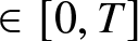 $\in[0,T]$, twice continuously differentiable for $x\in \mathbb{R}$, first continuously differentiable for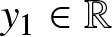 $y_{1}\in \mathbb{R}$ and first continuously differentiable for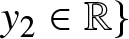 $y_{2}\in \mathbb{R}\}$. We use this definition to derive the alpha-robust Nash equilibrium reinsurance-investment strategy under the compound Poisson risk model. Since the mean-variance criterion lacks time-consistency, the classical Bellman optimality principle is not directly applicable. Therefore, we adopt a game-theoretic approach to find the time-consistent equilibrium strategy, which leads to the following extended HJB equation system. Next, we suppress the arguments of the control policies and the density generators for notational simplicity in the following paragraphs. For any functions $\varphi_{k}(t,x_{k},y_{k},y_{l},0),~\varphi_{k}(t,x_{k},y_{k},y_{l},1)\in C^{1,2,1,1}([0,T]\times \mathbb{R}\times \mathbb{R} \times \mathbb{R})$ where $k,~l\in\{1,2\},~k\neq l$, we define the infinitesimal generator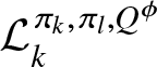 $\mathcal{L}^{\pi_{k},\pi_{l},Q^{\phi}}_{k}$ on $\varphi_{k}(t,\hat{x}_{k},y_{k},y_{l},h)$ under $\mathrm{Q}^{\phi}$ as follows:
 \begin{align}&\mathcal{L}^{\pi_{k},\pi^{*}_{l},Q^{\phi}}_{k}\varphi_{k}(t,\hat{x}_{k},y_{k},y_{l},h)\nonumber\\
&=\frac{\partial\varphi_{k}}{\partial t}+\bigg{[}A_{k}x^{\pi_k}_{k}-n_kA_{l}x^{\pi_l}_{l}+B_{k}y^{\pi_{k}}_{k}-n_kB_{l}y^{\pi_{l}}_{l}+C_{k}z^{\pi_{k}}_{k}-n_kC_{l}z^{\pi_{l}}_{l}\nonumber\\
&+d_{k}-(\lambda_k+\lambda)(1-q_{k})\mu_k-\theta_k(1-q_{k})^{2}(\lambda_k+\lambda)\sigma^{2}_{k}-n_kd_{l}+n_k(\lambda_l+\lambda)(1-q^{*}_{l})\mu_l\nonumber\\
&+n_k\theta_l(1-q^{*}_{l}(t))^{2}(\lambda_l+\lambda)\sigma^{2}_{l}+(\xi_{k}-n_k\xi^{*}_l(t))\alpha +(\omega_{k}-n_k\omega^{*}_{l}(t))(1-h)\eta(1-\Delta)\nonumber\\
&+(\phi_{k1}\xi_{k}-n_k\phi_{l1}\xi^{*}_{l}(t))\beta \bigg{]}\frac{\partial\varphi_{k}}{\partial\hat{x}_{k}}+({x}^{\pi^{k}}_{k}-\alpha_{k}y_{k}-e^{\alpha_{k}u_{k}}z_{k})\frac{\partial\varphi_{k}}{\partial y_{k}}\nonumber\\
&+({x}^{\pi_l}_{l}-\alpha_{k}y_{l}-e^{\alpha_{l}u_{l}}z_{l})\frac{\partial\varphi_{k}}{\partial y_{l}}+\frac{1}{2}(\xi_{k}-n_k\xi^{*}_l(t))^{2}\beta^2\frac{\partial^{2}\varphi_{k}}{\partial\hat{x}_{k}^{2}}\nonumber\\
&+\bigg{(}\varphi_{k}(t,\hat{x}_{k}-\zeta(\omega_{k}(t)-n_k\omega^{*}_{l}(t)),l,y_{k},y_{l},h+1)-\varphi_{k}(t,\hat{x}_{k},l,y_{k},y_{l},h)\bigg{)}h^{p}(1-h)\phi_{k2}\nonumber\\
&+\int^{\infty}_{0}\bigg{(}\varphi_{k}(t,\hat{x}_{k}-q_{k}y_{k},l,y_{k},y_{l},h+1)-\varphi_{k}(t,\hat{x}_{k},l,y_{k},y_{l},h)\bigg{)}(1-\phi_{k3}(t,y_{k}))\upsilon_{k}(dy_{k})\nonumber\\
&+\int^{\infty}_{0}\bigg{(}\varphi_{k}(t,\hat{x}_{k}-q_{k}y_{k},l,y_{k},y_{l},h+1)-\varphi_{k}(t,\hat{x}_{k},l,y_{k},y_{l},h)\bigg{)}(1-\phi_{k4}(t,y_{k}))\upsilon(dy_{k})\nonumber\\
&+\int^{\infty}_{0}\bigg{(}\varphi_{k}(t,\hat{x}_{k}+n_{k}q^{*}_{l}(t)y_{l},l,y_{k},y_{l},h)-\varphi_{k}(t,\hat{x}_{k},l,y_{k},y_{l},h)\bigg{)}(1-\phi^{*}_{l3}(t,y_{k}))\upsilon_{l}(dy_{l})\nonumber\\
&+\int^{\infty}_{0}\bigg{(}\varphi_{k}(t,\hat{x}_{k}+n_{k}q^{*}_{l}(t)y_{l},l,y_{l},h+1)-\varphi_{k}(t,\hat{x}_{k},l,y_{k},y_{l},hl)\bigg{)}(1-\phi^{*}_{l4}(t,y_{l}))\upsilon(dy_{l}),\end{align}
\begin{align}&\mathcal{L}^{\pi_{k},\pi^{*}_{l},Q^{\phi}}_{k}\varphi_{k}(t,\hat{x}_{k},y_{k},y_{l},h)\nonumber\\
&=\frac{\partial\varphi_{k}}{\partial t}+\bigg{[}A_{k}x^{\pi_k}_{k}-n_kA_{l}x^{\pi_l}_{l}+B_{k}y^{\pi_{k}}_{k}-n_kB_{l}y^{\pi_{l}}_{l}+C_{k}z^{\pi_{k}}_{k}-n_kC_{l}z^{\pi_{l}}_{l}\nonumber\\
&+d_{k}-(\lambda_k+\lambda)(1-q_{k})\mu_k-\theta_k(1-q_{k})^{2}(\lambda_k+\lambda)\sigma^{2}_{k}-n_kd_{l}+n_k(\lambda_l+\lambda)(1-q^{*}_{l})\mu_l\nonumber\\
&+n_k\theta_l(1-q^{*}_{l}(t))^{2}(\lambda_l+\lambda)\sigma^{2}_{l}+(\xi_{k}-n_k\xi^{*}_l(t))\alpha +(\omega_{k}-n_k\omega^{*}_{l}(t))(1-h)\eta(1-\Delta)\nonumber\\
&+(\phi_{k1}\xi_{k}-n_k\phi_{l1}\xi^{*}_{l}(t))\beta \bigg{]}\frac{\partial\varphi_{k}}{\partial\hat{x}_{k}}+({x}^{\pi^{k}}_{k}-\alpha_{k}y_{k}-e^{\alpha_{k}u_{k}}z_{k})\frac{\partial\varphi_{k}}{\partial y_{k}}\nonumber\\
&+({x}^{\pi_l}_{l}-\alpha_{k}y_{l}-e^{\alpha_{l}u_{l}}z_{l})\frac{\partial\varphi_{k}}{\partial y_{l}}+\frac{1}{2}(\xi_{k}-n_k\xi^{*}_l(t))^{2}\beta^2\frac{\partial^{2}\varphi_{k}}{\partial\hat{x}_{k}^{2}}\nonumber\\
&+\bigg{(}\varphi_{k}(t,\hat{x}_{k}-\zeta(\omega_{k}(t)-n_k\omega^{*}_{l}(t)),l,y_{k},y_{l},h+1)-\varphi_{k}(t,\hat{x}_{k},l,y_{k},y_{l},h)\bigg{)}h^{p}(1-h)\phi_{k2}\nonumber\\
&+\int^{\infty}_{0}\bigg{(}\varphi_{k}(t,\hat{x}_{k}-q_{k}y_{k},l,y_{k},y_{l},h+1)-\varphi_{k}(t,\hat{x}_{k},l,y_{k},y_{l},h)\bigg{)}(1-\phi_{k3}(t,y_{k}))\upsilon_{k}(dy_{k})\nonumber\\
&+\int^{\infty}_{0}\bigg{(}\varphi_{k}(t,\hat{x}_{k}-q_{k}y_{k},l,y_{k},y_{l},h+1)-\varphi_{k}(t,\hat{x}_{k},l,y_{k},y_{l},h)\bigg{)}(1-\phi_{k4}(t,y_{k}))\upsilon(dy_{k})\nonumber\\
&+\int^{\infty}_{0}\bigg{(}\varphi_{k}(t,\hat{x}_{k}+n_{k}q^{*}_{l}(t)y_{l},l,y_{k},y_{l},h)-\varphi_{k}(t,\hat{x}_{k},l,y_{k},y_{l},h)\bigg{)}(1-\phi^{*}_{l3}(t,y_{k}))\upsilon_{l}(dy_{l})\nonumber\\
&+\int^{\infty}_{0}\bigg{(}\varphi_{k}(t,\hat{x}_{k}+n_{k}q^{*}_{l}(t)y_{l},l,y_{l},h+1)-\varphi_{k}(t,\hat{x}_{k},l,y_{k},y_{l},hl)\bigg{)}(1-\phi^{*}_{l4}(t,y_{l}))\upsilon(dy_{l}),\end{align}Theorem 4.1. Verification theorem for Problem 1: If there exist  $V_{k}(t,\hat{x}_{k},y_{k},y_{l},h)$, and $\underline{g}_{k}(t,\hat{x}_{k},y_{k},y_{l},h)$, $\overline{g}_{k}(t,\hat{x}_{k},y_{k},y_{l},h)\in C^{1,2,2,1,1}([0,T]\times \mathbb{R}\times \mathbb{R}\times \mathbb{R} \times \mathbb{R})$ satisfying the following conditions:
(1)  $\forall (t,\hat{x}_{k},y_{k},y_{l})\in [0,T]\times \mathbb{R}\times \mathbb{R}\times \mathbb{R} \times \mathbb{R}$,
 \begin{align}
&\sup\limits_{\pi_{k}\in\Pi_{k}}\bigg{\{}\alpha_k\inf_{\underline{\phi}_{k\in\Phi_{k}}}\bigg{[}\mathcal{L}^{\pi_{k},\pi^{*}_{l},Q^{\underline{\phi}_{k}}}V_{k}(t,\hat{x}_{k},y_{k},y_{l},h)-\frac{\gamma_k}{2}\mathcal{L}^{\pi_{k},\pi^{*}_{l},Q^{\underline{\phi}_{k}}}\underline{g}^{2}_{k}(t,\hat{x}_{k},y_{k},y_{l},h)\nonumber\\
&+\gamma_k \underline{g}_{k}(t,\hat{x}_{k},y_{k},y_{l},h)\mathcal{L}^{\pi_{k},\pi^{*}_{l},Q^{\underline{\phi}_{k}}}\underline{g}_{k}(t,\hat{x}_{k},y_{k},y_{l},h)+h_{\beta}(\underline{\phi}_{k})\bigg{]}\nonumber\\
&+\hat{\alpha}_k\sup_{\overline{\phi}_{k\in\Phi_{k}}}\bigg{[}\mathcal{L}^{\pi_{k},\pi^{*}_{l},Q^{\overline{\phi}_{k}}}V_{k}(t,\hat{x}_{k},y_{k},y_{l},h)-\frac{\gamma_k}{2}\mathcal{L}^{\pi_{k},\pi^{*}_{l},Q^{\overline{\phi}_{k}}}\overline{g}^{2}_{k}(t,\hat{x}_{k},y_{k},y_{l},h)\nonumber\\
&+\gamma_k \overline{g}_{k}(t,\hat{x}_{k},y_{k},y_{l},h)\mathcal{L}^{\pi_{k},\pi^{*}_{l},Q^{\overline{\phi}_{k}}}\overline{g}_{k}(t,\hat{x}_{k},y_{k},y_{l},h)+h_{\beta}(\overline{\phi}_{k})\bigg{]}\bigg{\}}=0,
\end{align}
\begin{align}
&\sup\limits_{\pi_{k}\in\Pi_{k}}\bigg{\{}\alpha_k\inf_{\underline{\phi}_{k\in\Phi_{k}}}\bigg{[}\mathcal{L}^{\pi_{k},\pi^{*}_{l},Q^{\underline{\phi}_{k}}}V_{k}(t,\hat{x}_{k},y_{k},y_{l},h)-\frac{\gamma_k}{2}\mathcal{L}^{\pi_{k},\pi^{*}_{l},Q^{\underline{\phi}_{k}}}\underline{g}^{2}_{k}(t,\hat{x}_{k},y_{k},y_{l},h)\nonumber\\
&+\gamma_k \underline{g}_{k}(t,\hat{x}_{k},y_{k},y_{l},h)\mathcal{L}^{\pi_{k},\pi^{*}_{l},Q^{\underline{\phi}_{k}}}\underline{g}_{k}(t,\hat{x}_{k},y_{k},y_{l},h)+h_{\beta}(\underline{\phi}_{k})\bigg{]}\nonumber\\
&+\hat{\alpha}_k\sup_{\overline{\phi}_{k\in\Phi_{k}}}\bigg{[}\mathcal{L}^{\pi_{k},\pi^{*}_{l},Q^{\overline{\phi}_{k}}}V_{k}(t,\hat{x}_{k},y_{k},y_{l},h)-\frac{\gamma_k}{2}\mathcal{L}^{\pi_{k},\pi^{*}_{l},Q^{\overline{\phi}_{k}}}\overline{g}^{2}_{k}(t,\hat{x}_{k},y_{k},y_{l},h)\nonumber\\
&+\gamma_k \overline{g}_{k}(t,\hat{x}_{k},y_{k},y_{l},h)\mathcal{L}^{\pi_{k},\pi^{*}_{l},Q^{\overline{\phi}_{k}}}\overline{g}_{k}(t,\hat{x}_{k},y_{k},y_{l},h)+h_{\beta}(\overline{\phi}_{k})\bigg{]}\bigg{\}}=0,
\end{align}where  $(\pi^{*}_{k},\underline{\phi}^{*}_{k},\overline{\phi}^{*}_{k})$ denote the optimal strategy and probability distortion functions, respectively,
 \begin{equation}
\begin{aligned}
(\pi^{*}_{k},\underline{\phi}^{*}_{k},\overline{\phi}^{*}_{k})=&\arg\sup\limits_{\pi_{k}\in\Pi_{k}}\bigg{\{}\alpha_k\arg\inf_{\underline{\phi}_{k\in\Phi_{k}}}\bigg{[}\mathcal{L}^{\pi_{k},\pi^{*}_{l},Q^{\underline{\phi}_{k}}}V_{k}(t,\hat{x}_{k},y_{k},y_{l},h)-\frac{\gamma_k}{2}\mathcal{L}^{\pi_{k},\pi^{*}_{l},Q^{\underline{\phi}_{k}}}\underline{g}^{2}_{k}(t,\hat{x}_{k},y_{k},y_{l},h)\\
&+\gamma_k \underline{g}_{k}(t,\hat{x}_{k},y_{k},y_{l},h)\mathcal{L}^{\pi_{k},\pi^{*}_{l},Q^{\underline{\phi}_{k}}}\underline{g}_{k}(t,\hat{x}_{k},y_{k},y_{l},h)+h_{\beta}(\underline{\phi}_{k})\bigg{]}\\
&+\hat{\alpha}_k\arg\sup_{\overline{\phi}_{k\in\Phi_{k}}}\bigg{[}\mathcal{L}^{\pi_{k},\pi^{*}_{l},Q^{\overline{\phi}_{k}}}V_{k}(t,\hat{x}_{k},y_{k},y_{l},h)-\frac{\gamma_k}{2}\mathcal{L}^{\pi_{k},\pi^{*}_{l},Q^{\overline{\phi}_{k}}}\overline{g}^{2}_{k}(t,\hat{x}_{k},y_{k},y_{l},h)\\
&+\gamma \overline{g}_{k}(t,\hat{x}_{k},y_{k},y_{l},h)\mathcal{L}^{\pi_{k},\pi^{*}_{l},Q^{\overline{\phi}_{k}}}\overline{g}_{k}(t,\hat{x}_{k},y_{k},y_{l},h)+h_{\beta}(\overline{\phi}_{k})\bigg{]}\bigg{\}}.\\
\end{aligned}
\end{equation}
\begin{equation}
\begin{aligned}
(\pi^{*}_{k},\underline{\phi}^{*}_{k},\overline{\phi}^{*}_{k})=&\arg\sup\limits_{\pi_{k}\in\Pi_{k}}\bigg{\{}\alpha_k\arg\inf_{\underline{\phi}_{k\in\Phi_{k}}}\bigg{[}\mathcal{L}^{\pi_{k},\pi^{*}_{l},Q^{\underline{\phi}_{k}}}V_{k}(t,\hat{x}_{k},y_{k},y_{l},h)-\frac{\gamma_k}{2}\mathcal{L}^{\pi_{k},\pi^{*}_{l},Q^{\underline{\phi}_{k}}}\underline{g}^{2}_{k}(t,\hat{x}_{k},y_{k},y_{l},h)\\
&+\gamma_k \underline{g}_{k}(t,\hat{x}_{k},y_{k},y_{l},h)\mathcal{L}^{\pi_{k},\pi^{*}_{l},Q^{\underline{\phi}_{k}}}\underline{g}_{k}(t,\hat{x}_{k},y_{k},y_{l},h)+h_{\beta}(\underline{\phi}_{k})\bigg{]}\\
&+\hat{\alpha}_k\arg\sup_{\overline{\phi}_{k\in\Phi_{k}}}\bigg{[}\mathcal{L}^{\pi_{k},\pi^{*}_{l},Q^{\overline{\phi}_{k}}}V_{k}(t,\hat{x}_{k},y_{k},y_{l},h)-\frac{\gamma_k}{2}\mathcal{L}^{\pi_{k},\pi^{*}_{l},Q^{\overline{\phi}_{k}}}\overline{g}^{2}_{k}(t,\hat{x}_{k},y_{k},y_{l},h)\\
&+\gamma \overline{g}_{k}(t,\hat{x}_{k},y_{k},y_{l},h)\mathcal{L}^{\pi_{k},\pi^{*}_{l},Q^{\overline{\phi}_{k}}}\overline{g}_{k}(t,\hat{x}_{k},y_{k},y_{l},h)+h_{\beta}(\overline{\phi}_{k})\bigg{]}\bigg{\}}.\\
\end{aligned}
\end{equation} (2)  $\forall (t,\hat{x}_{k},y_{k},y_{l})\in [0,T]\times \mathbb{R}\times \mathbb{R}\times \mathbb{R} \times \mathbb{R}$,
 \begin{equation*}\qquad\qquad\qquad\qquad\qquad
\begin{cases}
& V_{k}(T,\hat{x}_{k},y_{k},y_{l},h)=\hat{x}_{k}+\vartheta_{k}y_{k}-n_{k}\vartheta_{l}y_{l}, \qquad\qquad\qquad\qquad\qquad\quad\text{(4.5a)}\\
& \mathcal{L}^{\pi^{*}_{k},\pi^{*}_{l},Q^{\underline{\phi}_{k}}}\underline{g}_{k}(t,\hat{x}_{k},y_{k},y_{l},h)=0, \qquad\qquad\qquad\qquad\qquad\qquad\quad\,\,\ \ \text{(4.5b)} \\
& \underline{g}_{k}(T,\hat{x}_{k},y_{k},y_{l},h)=\hat{x}_{k}+\vartheta_{k}y_{k}-n_{k}\vartheta_{l}y_{l}, \qquad\qquad\qquad\qquad\qquad\quad\text{(4.5c)}\\
&\mathcal{L}^{\pi^{*}_{k},\pi^{*}_{l}Q^{\overline{\phi}_{k}}}\overline{g}(t,\hat{x}_{k},y_{k},y_{l},h)=0, \qquad\qquad\qquad\qquad\qquad\quad\quad\quad\quad\,\, \ \text{(4.5d)} \\
&\overline{g}_{k}(T,\hat{x}_{k},y_{k},y_{l},h)=\hat{x}_{k}+\vartheta_{k}y_{k}-n_{k}\vartheta_{l}y_{l}, \qquad\qquad\qquad\qquad\qquad\quad\text{(4.5e)}
\end{cases}
\end{equation*}
\begin{equation*}\qquad\qquad\qquad\qquad\qquad
\begin{cases}
& V_{k}(T,\hat{x}_{k},y_{k},y_{l},h)=\hat{x}_{k}+\vartheta_{k}y_{k}-n_{k}\vartheta_{l}y_{l}, \qquad\qquad\qquad\qquad\qquad\quad\text{(4.5a)}\\
& \mathcal{L}^{\pi^{*}_{k},\pi^{*}_{l},Q^{\underline{\phi}_{k}}}\underline{g}_{k}(t,\hat{x}_{k},y_{k},y_{l},h)=0, \qquad\qquad\qquad\qquad\qquad\qquad\quad\,\,\ \ \text{(4.5b)} \\
& \underline{g}_{k}(T,\hat{x}_{k},y_{k},y_{l},h)=\hat{x}_{k}+\vartheta_{k}y_{k}-n_{k}\vartheta_{l}y_{l}, \qquad\qquad\qquad\qquad\qquad\quad\text{(4.5c)}\\
&\mathcal{L}^{\pi^{*}_{k},\pi^{*}_{l}Q^{\overline{\phi}_{k}}}\overline{g}(t,\hat{x}_{k},y_{k},y_{l},h)=0, \qquad\qquad\qquad\qquad\qquad\quad\quad\quad\quad\,\, \ \text{(4.5d)} \\
&\overline{g}_{k}(T,\hat{x}_{k},y_{k},y_{l},h)=\hat{x}_{k}+\vartheta_{k}y_{k}-n_{k}\vartheta_{l}y_{l}, \qquad\qquad\qquad\qquad\qquad\quad\text{(4.5e)}
\end{cases}
\end{equation*} (3) 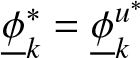 $\underline{\phi}^{*}_{k}=\underline{\phi}^{u^{*}}_{k}$ and $\overline{\phi}^{*}_{k}=\overline{\phi}^{u^{*}}_{k}$.
Then  $\pi^{*}_{k}(t)$ is the equilibrium strategy and $V_{k}(t,\hat{x}_{k},y_{k},y_{l},h)=J^{\pi_k,\pi^{*}_l}_{k}(t,\hat{x}_{k},y_{k},y_{l},h)$ is the equilibrium value function to $alpha$-robust reinsurance-reinsurance problem. Besides, $\underline{g}_{k}(T,\hat{x}_{k},y_{k},y_{l},h)=\mathrm{E}^{\underline{\phi}^{*}_{k}}_{t,x, y_{k},y_{l},h}[\hat{X}^{\pi_{k},\pi_{l}}_{k}(T)]$ and $\overline{g}_{k}(T,\hat{x}_{k},y_{k},y_{l},h)=\mathrm{E}^{\overline{\phi}^{*}_{k}}_{t,x, y_{k},y_{l},h}[\hat{X}^{\pi_{k},\pi_{l}}_{k}(T)]$.
We solve the extended HJB system of equations in two steps.
Step 1: We divide the extended HJB system of equations (4.3) and (4.5) into two parts that represent the pre- and post-default value functions:
 \begin{equation}
V_{k}(t,\hat{x}_{k},y_{k},y_{l},h)=\left\{
\begin{aligned}
&V_{k}(t,\hat{x}_{k},y_{k},y_{l},0),~~~\mathrm{if}~~h=0~~\text{(~pre-default~case)},\\
&V_{k}(t,\hat{x}_{k},y_{k},y_{l},1),~~~\mathrm{if}~~h=1~~\text{(~post-default~case)},
\end{aligned}
\right.
\end{equation}
\begin{equation}
V_{k}(t,\hat{x}_{k},y_{k},y_{l},h)=\left\{
\begin{aligned}
&V_{k}(t,\hat{x}_{k},y_{k},y_{l},0),~~~\mathrm{if}~~h=0~~\text{(~pre-default~case)},\\
&V_{k}(t,\hat{x}_{k},y_{k},y_{l},1),~~~\mathrm{if}~~h=1~~\text{(~post-default~case)},
\end{aligned}
\right.
\end{equation} \begin{equation}
\underline{g}_{k}(t,\hat{x}_{k},y_{k},y_{l},h)=\left\{
\begin{aligned}
&\underline{g}_{k}(t,\hat{x}_{k},y_{k},y_{l},0),~~~\mathrm{if}~~h=0~\text{~(~pre-default~case)},\\
&\underline{g}_{k}(t,\hat{x}_{k},y_{k},y_{l},1),~~~\mathrm{if}~~h=1~~\text{(~post-default~case)},
\end{aligned}
\right.
\end{equation}
\begin{equation}
\underline{g}_{k}(t,\hat{x}_{k},y_{k},y_{l},h)=\left\{
\begin{aligned}
&\underline{g}_{k}(t,\hat{x}_{k},y_{k},y_{l},0),~~~\mathrm{if}~~h=0~\text{~(~pre-default~case)},\\
&\underline{g}_{k}(t,\hat{x}_{k},y_{k},y_{l},1),~~~\mathrm{if}~~h=1~~\text{(~post-default~case)},
\end{aligned}
\right.
\end{equation} \begin{equation}
\overline{g}_{k}(t,\hat{x}_{k},y_{k},y_{l},h)=\left\{
\begin{aligned}
&\overline{g}_{k}(t,\hat{x}_{k},y_{k},y_{l},0),~~~\mathrm{if}~~h=0~~\text{(~pre-default~case)},\\
&\overline{g}_{k}(t,\hat{x}_{k},y_{k},y_{l},1),~~~\mathrm{if}~~h=1~~\text{(~post-default~case)}.
\end{aligned}
\right.
\end{equation}
\begin{equation}
\overline{g}_{k}(t,\hat{x}_{k},y_{k},y_{l},h)=\left\{
\begin{aligned}
&\overline{g}_{k}(t,\hat{x}_{k},y_{k},y_{l},0),~~~\mathrm{if}~~h=0~~\text{(~pre-default~case)},\\
&\overline{g}_{k}(t,\hat{x}_{k},y_{k},y_{l},1),~~~\mathrm{if}~~h=1~~\text{(~post-default~case)}.
\end{aligned}
\right.
\end{equation}Step 2: We reduce the extended HJB system of equations into two simpler extended HJB systems of equations that are satisfied by the pre-default value function and the post-default value function, respectively. Then, we solve the HJB equation for the post-default value function using the standard dynamic programming approach.
4.1.1. Solution to non-zero-sum game after default (
$h=1$)

In this subsection, we derive the non-zero-sum game reinsurance-investment strategy to describe the insurers’ strategic interactions with relative performance concerns after default.
Theorem 4.2 (Post-default)
Consider the  $\alpha$-robust game between two ambiguity-averse insurers with mean-variance utility described in Problem 1. For any $t\in[T\wedge\tau,T]$, the time-consistent Nash equilibrium strategy of insurer $k$, for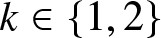 $k\in\{1,2\}$, can be described as follows:
(1) The non-zero-sum differential game reinsurance strategy  $q^{*}_{k}$ is determined by the following equation:
 \begin{equation}
\begin{aligned}
&[(\lambda_{k}+\lambda)(\mu_{k}+2\theta_{k}(1-q^{*}_{k})\sigma_{k}^{2})]E_{k}(t)\\
&-\int^{\infty}_{0}(\hat{\alpha}_{k}\exp(-\beta_{k3}{X^{*}_{k}})+\alpha_{k}\exp(\beta_{k3}{X^{*}_{k}}))(E_{k}(t)y_{k}+\gamma_{k}{e}^{2}_{k}y^{2}_{k}q^{*}_{k})\upsilon_{k}(dy_{k})\\
&-\int^{\infty}_{0}(\hat{\alpha}_{k}\exp(-\beta_{k4}{X^{*}_{k}})+\alpha_{k}\exp(\beta_{k4}{X^{*}_{k}})(E_{k}(t)y_{k}+\gamma_{k}{e}^{2}_{k}y^{2}_{k}q^{*}_{k})\upsilon(dy_{k})=0,
\end{aligned}
\end{equation}
\begin{equation}
\begin{aligned}
&[(\lambda_{k}+\lambda)(\mu_{k}+2\theta_{k}(1-q^{*}_{k})\sigma_{k}^{2})]E_{k}(t)\\
&-\int^{\infty}_{0}(\hat{\alpha}_{k}\exp(-\beta_{k3}{X^{*}_{k}})+\alpha_{k}\exp(\beta_{k3}{X^{*}_{k}}))(E_{k}(t)y_{k}+\gamma_{k}{e}^{2}_{k}y^{2}_{k}q^{*}_{k})\upsilon_{k}(dy_{k})\\
&-\int^{\infty}_{0}(\hat{\alpha}_{k}\exp(-\beta_{k4}{X^{*}_{k}})+\alpha_{k}\exp(\beta_{k4}{X^{*}_{k}})(E_{k}(t)y_{k}+\gamma_{k}{e}^{2}_{k}y^{2}_{k}q^{*}_{k})\upsilon(dy_{k})=0,
\end{aligned}
\end{equation}(2) The non-zero-sum differential game investment strategy for stock assets is given by
 \begin{equation}
\xi^{*}_{k}=\frac{\frac{\alpha E_{k}(t)}{\overline{A_{k}}(t)+\overline{B_{k}}(t)}+\frac{\alpha E_{l}(t)}{\overline{A_{l}}(t)+\overline{B_{l}}(t)}\frac{n_{k}\overline{A_{k}}(t)}{\overline{A_{k}}(t)+\overline{B_{k}}(t)}}{1-\frac{n_{k}\overline{A_{k}}(t)}{\overline{A_{k}}(t)+\overline{B_{k}}(t)}\frac{n_{l}\overline{A_{l}}(t)}{\overline{A_{l}}(t)+\overline{B_{l}}(t)}}\triangleq\overline{D^{\pi_{k}}_{kl}}(t),
\end{equation}
\begin{equation}
\xi^{*}_{k}=\frac{\frac{\alpha E_{k}(t)}{\overline{A_{k}}(t)+\overline{B_{k}}(t)}+\frac{\alpha E_{l}(t)}{\overline{A_{l}}(t)+\overline{B_{l}}(t)}\frac{n_{k}\overline{A_{k}}(t)}{\overline{A_{k}}(t)+\overline{B_{k}}(t)}}{1-\frac{n_{k}\overline{A_{k}}(t)}{\overline{A_{k}}(t)+\overline{B_{k}}(t)}\frac{n_{l}\overline{A_{l}}(t)}{\overline{A_{l}}(t)+\overline{B_{l}}(t)}}\triangleq\overline{D^{\pi_{k}}_{kl}}(t),
\end{equation}where
 \begin{equation}
\begin{aligned}
&\overline{A_{k}}(t)=\gamma_k\beta^{2}\exp(2(A_{k}+\vartheta_{k})(T-t)),~\overline{B_{k}}(t)=(\hat{\alpha}_{k}-\alpha_{k})\beta_{k1}\beta^{2}\exp(2(A_{k}+\vartheta_{k})(T-t)),
\end{aligned}
\end{equation}
\begin{equation}
\begin{aligned}
&\overline{A_{k}}(t)=\gamma_k\beta^{2}\exp(2(A_{k}+\vartheta_{k})(T-t)),~\overline{B_{k}}(t)=(\hat{\alpha}_{k}-\alpha_{k})\beta_{k1}\beta^{2}\exp(2(A_{k}+\vartheta_{k})(T-t)),
\end{aligned}
\end{equation}(3) The non-zero-sum differential game investment strategy for corporate bonds is given by
 \begin{equation}
\omega^{*}_{k}=0,~~{k}\neq l\in\{1,2\}.
\end{equation}
\begin{equation}
\omega^{*}_{k}=0,~~{k}\neq l\in\{1,2\}.
\end{equation} Additionally, the equilibrium value function of insurer  $k$ is given by
 \begin{equation}
V_{k}(t,\hat{x}_{k},y_{k},y_{l},h)=(\hat{x}_{k}+\vartheta_{k}y_{k}-n_{k}\vartheta_{l}y_{l})\exp((A_{k}+\vartheta_{k})(T-t))+{H_{k}(t)},
\end{equation}
\begin{equation}
V_{k}(t,\hat{x}_{k},y_{k},y_{l},h)=(\hat{x}_{k}+\vartheta_{k}y_{k}-n_{k}\vartheta_{l}y_{l})\exp((A_{k}+\vartheta_{k})(T-t))+{H_{k}(t)},
\end{equation}where  $k\neq l\in\{1,2\}$, and
 \begin{equation}
\begin{aligned}
{H}_{k}(t)&=\int^{T}_{t}\bigg{[}d_{k}-(\lambda_k+\lambda)(1-q^{*}_{k}(s))\mu_k-\theta_k(1-q^{*}_{k}(s))^{2}(\lambda_k+\lambda)\sigma^{2}_{k}-n_kd_{l}+n_k(\lambda_l+\lambda)(1-q^{*}_{l}(s))\mu_l\\
&+n_k\theta_l(1-q^{*}_{l}(s))^{2}(\lambda_l+\lambda)\sigma^{2}_{l}+(\overline{D^{\pi_{k}}_{kl}}(s)-n_k\overline{D^{\pi_{l}}_{lk}}(s))\alpha E_{k}(s)-n_k(\hat{\alpha}_{k}-\alpha_{k})\overline{D^{\pi_{l}}_{lk}}(s)^{2}\beta^{2}E_{l}(t) E_{k}(s)\\
&-\frac{\gamma}{2}(\overline{D^{\pi_{k}}_{kl}}(s)-n_k\overline{D^{\pi_{l}}_{lk}}(s))^{2}\beta^2(\alpha_{k}\underline{e_{k}^{2}}(s)+\hat{\alpha}_{k}\overline{e_{k}}^{2}(s))+\frac{(\hat{\alpha_{k}}-\alpha_{k})}{2}\beta_{k1}\beta^{2}\overline{D^{\pi_{k}}_{kl}}(s)E^{2}_{k}(s)\\
&+\alpha_{k}\int^{\infty}_{0}\bigg{[}1-\exp(\beta_{k3}\underline{X^{*}_{k}})\bigg{]}\upsilon_{k}(dy_{k})+\alpha_{k}\int^{\infty}_{0}\bigg{[}1-\exp(\beta_{k4}\underline{X^{*}_{k}})\bigg{]}\upsilon(dy_{k})\\
&+\hat{\alpha}_{k}\int^{\infty}_{0}\bigg{[}1-\exp(-\beta_{k3}\overline{X^{*}_{k}})\bigg{]}\upsilon_{k}(dy_{k})+\hat{\alpha}_{k}\int^{\infty}_{0}\bigg{[}1-\exp(-\beta_{k4}\overline{X^{*}_{k}})\bigg{]}\upsilon(dy_{k})\\
&+\alpha_{k}\int^{\infty}_{0}\bigg{(}n_{k}E_{k}(s)q^{*}_{l}(s)y_{l}-\frac{\gamma_k}{2}n^{2}_{k}\underline{e^{2}_{k}}(s)(q^{*}_{l}(s))^{2}y^{2}_{l}\bigg{)}\exp(\beta_{l3}\underline{X^{*}_{l}})\upsilon_{l}(dy_{l})\\
&+\alpha_{k}\int^{\infty}_{0}\bigg{(}n_{k}E_{k}(s)q^{*}_{l}(s)y_{l}-\frac{\gamma_k}{2}n^{2}_{k}\underline{e^{2}_{k}}(s)(q^{*}_{l}(s))^{2}y^{2}_{l}\bigg{)}\exp(\beta_{l4}\underline{X^{*}_{l}})\upsilon(dy_{l})\\
&+\hat{\alpha_{k}}\int^{\infty}_{0}\bigg{(}n_{k}E_{k}(s)q^{*}_{l}(s)y_{l}-\frac{\gamma_k}{2}n^{2}_{k}\overline{e_{k}}^{2}(s)(q^{*}_{l}(s))^{2}y^{2}_{l}\bigg{)}\exp(-\beta_{l3}\overline{X^{*}_{l}})\upsilon_{l}(dy_{l})\\
&+\hat{\alpha_{k}}\int^{\infty}_{0}\bigg{(}n_{k}E_{k}(s)q^{*}_{l}(s)y_{l}-\frac{\gamma_k}{2}n^{2}_{k}\overline{e_{k}}^{2}(s)(q^{*}_{l}(s))^{2}y^{2}_{l}\bigg{)}\exp(-\beta_{l4}\overline{X^{*}_{l}})\upsilon(dy_{l})\bigg{]}ds,\\
\end{aligned}
\end{equation}
\begin{equation}
\begin{aligned}
{H}_{k}(t)&=\int^{T}_{t}\bigg{[}d_{k}-(\lambda_k+\lambda)(1-q^{*}_{k}(s))\mu_k-\theta_k(1-q^{*}_{k}(s))^{2}(\lambda_k+\lambda)\sigma^{2}_{k}-n_kd_{l}+n_k(\lambda_l+\lambda)(1-q^{*}_{l}(s))\mu_l\\
&+n_k\theta_l(1-q^{*}_{l}(s))^{2}(\lambda_l+\lambda)\sigma^{2}_{l}+(\overline{D^{\pi_{k}}_{kl}}(s)-n_k\overline{D^{\pi_{l}}_{lk}}(s))\alpha E_{k}(s)-n_k(\hat{\alpha}_{k}-\alpha_{k})\overline{D^{\pi_{l}}_{lk}}(s)^{2}\beta^{2}E_{l}(t) E_{k}(s)\\
&-\frac{\gamma}{2}(\overline{D^{\pi_{k}}_{kl}}(s)-n_k\overline{D^{\pi_{l}}_{lk}}(s))^{2}\beta^2(\alpha_{k}\underline{e_{k}^{2}}(s)+\hat{\alpha}_{k}\overline{e_{k}}^{2}(s))+\frac{(\hat{\alpha_{k}}-\alpha_{k})}{2}\beta_{k1}\beta^{2}\overline{D^{\pi_{k}}_{kl}}(s)E^{2}_{k}(s)\\
&+\alpha_{k}\int^{\infty}_{0}\bigg{[}1-\exp(\beta_{k3}\underline{X^{*}_{k}})\bigg{]}\upsilon_{k}(dy_{k})+\alpha_{k}\int^{\infty}_{0}\bigg{[}1-\exp(\beta_{k4}\underline{X^{*}_{k}})\bigg{]}\upsilon(dy_{k})\\
&+\hat{\alpha}_{k}\int^{\infty}_{0}\bigg{[}1-\exp(-\beta_{k3}\overline{X^{*}_{k}})\bigg{]}\upsilon_{k}(dy_{k})+\hat{\alpha}_{k}\int^{\infty}_{0}\bigg{[}1-\exp(-\beta_{k4}\overline{X^{*}_{k}})\bigg{]}\upsilon(dy_{k})\\
&+\alpha_{k}\int^{\infty}_{0}\bigg{(}n_{k}E_{k}(s)q^{*}_{l}(s)y_{l}-\frac{\gamma_k}{2}n^{2}_{k}\underline{e^{2}_{k}}(s)(q^{*}_{l}(s))^{2}y^{2}_{l}\bigg{)}\exp(\beta_{l3}\underline{X^{*}_{l}})\upsilon_{l}(dy_{l})\\
&+\alpha_{k}\int^{\infty}_{0}\bigg{(}n_{k}E_{k}(s)q^{*}_{l}(s)y_{l}-\frac{\gamma_k}{2}n^{2}_{k}\underline{e^{2}_{k}}(s)(q^{*}_{l}(s))^{2}y^{2}_{l}\bigg{)}\exp(\beta_{l4}\underline{X^{*}_{l}})\upsilon(dy_{l})\\
&+\hat{\alpha_{k}}\int^{\infty}_{0}\bigg{(}n_{k}E_{k}(s)q^{*}_{l}(s)y_{l}-\frac{\gamma_k}{2}n^{2}_{k}\overline{e_{k}}^{2}(s)(q^{*}_{l}(s))^{2}y^{2}_{l}\bigg{)}\exp(-\beta_{l3}\overline{X^{*}_{l}})\upsilon_{l}(dy_{l})\\
&+\hat{\alpha_{k}}\int^{\infty}_{0}\bigg{(}n_{k}E_{k}(s)q^{*}_{l}(s)y_{l}-\frac{\gamma_k}{2}n^{2}_{k}\overline{e_{k}}^{2}(s)(q^{*}_{l}(s))^{2}y^{2}_{l}\bigg{)}\exp(-\beta_{l4}\overline{X^{*}_{l}})\upsilon(dy_{l})\bigg{]}ds,\\
\end{aligned}
\end{equation}with
 \begin{equation}
\left\{
\begin{aligned}
&\overline{X^{*}_{k}}(t)=E_{k}(t)y_{k}q^{*}_{k}(t)+\frac{\gamma_{k}}{2}\overline{{e}_{k}}^{2}(t)y^{2}_{k}(q^{*}_{k}(t))^{2},\\
&\underline{X^{*}_{k}}(t)=E_{k}(t)y_{k}q^{*}_{k}(t)+\frac{\gamma_{k}}{2}\underline{{e}_{k}^{2}}(t)y^{2}_{k}(q^{*}_{k}(t))^{2},\\
&\overline{X^{*}_{l}}(t)=E_{l}(t)y_{l}q^{*}_{l}(t)+\frac{\gamma_{l}}{2}\overline{{e}_{l}}^{2}(t)y^{2}_{l}(q^{*}_{l}(t))^{2},\\
&\underline{X^{*}_{l}}(t)=E_{l}(t)y_{l}q^{*}_{l}(t)+\frac{\gamma_{l}}{2}\underline{{e}^{2}_{l}}(t)y^{2}_{l}(q^{*}_{l}(t))^{2},
\end{aligned}
\right.
\end{equation}
\begin{equation}
\left\{
\begin{aligned}
&\overline{X^{*}_{k}}(t)=E_{k}(t)y_{k}q^{*}_{k}(t)+\frac{\gamma_{k}}{2}\overline{{e}_{k}}^{2}(t)y^{2}_{k}(q^{*}_{k}(t))^{2},\\
&\underline{X^{*}_{k}}(t)=E_{k}(t)y_{k}q^{*}_{k}(t)+\frac{\gamma_{k}}{2}\underline{{e}_{k}^{2}}(t)y^{2}_{k}(q^{*}_{k}(t))^{2},\\
&\overline{X^{*}_{l}}(t)=E_{l}(t)y_{l}q^{*}_{l}(t)+\frac{\gamma_{l}}{2}\overline{{e}_{l}}^{2}(t)y^{2}_{l}(q^{*}_{l}(t))^{2},\\
&\underline{X^{*}_{l}}(t)=E_{l}(t)y_{l}q^{*}_{l}(t)+\frac{\gamma_{l}}{2}\underline{{e}^{2}_{l}}(t)y^{2}_{l}(q^{*}_{l}(t))^{2},
\end{aligned}
\right.
\end{equation}and
 \begin{equation}
E_{k}(t)={e_{k}}(t)=\underline{e_{k}}(t)=\overline{e_{k}}(t)=\exp((A_{k}+\vartheta_{k})(T-t)),~~k\neq l\in\{1,2\}.
\end{equation}
\begin{equation}
E_{k}(t)={e_{k}}(t)=\underline{e_{k}}(t)=\overline{e_{k}}(t)=\exp((A_{k}+\vartheta_{k})(T-t)),~~k\neq l\in\{1,2\}.
\end{equation} The expected value of each insurer’s relative surplus at terminal wealth under the probability measure  $\mathbb{Q}^{\underline{\phi}^{*}_{k}}$ is given by
 \begin{equation}
\underline{g}_{k}(t,\hat{x}_{k},y_{k},y_{l},h)=(\hat{x}_{k}+\vartheta_{k}y_{k}-n_{k}\vartheta_{l}y_{l})\exp((A_{k}+\vartheta_{k})(T-t))+\underline{h}_{k}(t),
\end{equation}
\begin{equation}
\underline{g}_{k}(t,\hat{x}_{k},y_{k},y_{l},h)=(\hat{x}_{k}+\vartheta_{k}y_{k}-n_{k}\vartheta_{l}y_{l})\exp((A_{k}+\vartheta_{k})(T-t))+\underline{h}_{k}(t),
\end{equation}where
 \begin{equation}
\begin{aligned}
\underline{{h}}_{k}(t)&=\int^{T}_{t}\bigg{[}d_{k}-(\lambda_k+\lambda)(1-q^{*}_{k}(s))\mu_k-\theta_k(1-q^{*}_{k}(s))^{2}(\lambda_k+\lambda)\sigma^{2}_{k}-n_kd_{l}+n_k(\lambda_l+\lambda)(1-q^{*}_{l}(s))\mu_l\\
&+n_k\theta_l(1-q^{*}_{l}(s))^{2}(\lambda_l+\lambda)\sigma^{2}_{l}+[(\overline{D^{\pi_{k}}_{kl}}(s)-n_k\overline{D^{\pi_{l}}_{lk}}(s))\alpha+(n_k\beta_{l1}\overline{D^{\pi_{l}}_{lk}}(s)-\beta_{k1}\overline{D^{\pi_{k}}_{kl}}(s))]\\
&\times\beta^{2}E_{k}(s)\underline{e_{k}}(s) -\int^{\infty}_{0}\underline{e_{k}}(s)q^{*}_{k}(s)y_{k}\exp(\beta_{k3}\underline{X^{*}_{k}})\upsilon_{k}(dy_{k})-\int^{\infty}_{0}\underline{e_{k}}(s)n_{k}q^{*}_{l}(s)y_{l}\exp(\beta_{l4}\underline{X^{*}_{l}})\upsilon_{k}(dy_{l})\\
&-\int^{\infty}_{0}\underline{e_{k}}(s)q^{*}_{k}(s)y_{k}\exp(\beta_{k4}\underline{X^{*}_{k}})\upsilon_{k}(dy_{k})-\int^{\infty}_{0}\underline{e_{k}}(s)n_{k}q^{*}_{l}(s)y_{l}\exp(\beta_{l3}\underline{X^{*}_{l}})\upsilon_{k}(dy_{l})\bigg{]}ds\\
\end{aligned}
\end{equation}
\begin{equation}
\begin{aligned}
\underline{{h}}_{k}(t)&=\int^{T}_{t}\bigg{[}d_{k}-(\lambda_k+\lambda)(1-q^{*}_{k}(s))\mu_k-\theta_k(1-q^{*}_{k}(s))^{2}(\lambda_k+\lambda)\sigma^{2}_{k}-n_kd_{l}+n_k(\lambda_l+\lambda)(1-q^{*}_{l}(s))\mu_l\\
&+n_k\theta_l(1-q^{*}_{l}(s))^{2}(\lambda_l+\lambda)\sigma^{2}_{l}+[(\overline{D^{\pi_{k}}_{kl}}(s)-n_k\overline{D^{\pi_{l}}_{lk}}(s))\alpha+(n_k\beta_{l1}\overline{D^{\pi_{l}}_{lk}}(s)-\beta_{k1}\overline{D^{\pi_{k}}_{kl}}(s))]\\
&\times\beta^{2}E_{k}(s)\underline{e_{k}}(s) -\int^{\infty}_{0}\underline{e_{k}}(s)q^{*}_{k}(s)y_{k}\exp(\beta_{k3}\underline{X^{*}_{k}})\upsilon_{k}(dy_{k})-\int^{\infty}_{0}\underline{e_{k}}(s)n_{k}q^{*}_{l}(s)y_{l}\exp(\beta_{l4}\underline{X^{*}_{l}})\upsilon_{k}(dy_{l})\\
&-\int^{\infty}_{0}\underline{e_{k}}(s)q^{*}_{k}(s)y_{k}\exp(\beta_{k4}\underline{X^{*}_{k}})\upsilon_{k}(dy_{k})-\int^{\infty}_{0}\underline{e_{k}}(s)n_{k}q^{*}_{l}(s)y_{l}\exp(\beta_{l3}\underline{X^{*}_{l}})\upsilon_{k}(dy_{l})\bigg{]}ds\\
\end{aligned}
\end{equation} The expected value of each insurer’s relative surplus at terminal wealth under the probability measure  $\mathrm{Q}^{\overline{\phi}^{*}_{k}}$ is given by
 \begin{equation}
\overline{g}_{k}(t,\hat{x}_{k},y_{k},y_{l},h)=(\hat{x}_{k}+\vartheta_{k}y_{k}-n_{k}\vartheta_{l}y_{l})\exp((A_{k}+\vartheta_{k})(T-t))+\overline{h}_{k}(t),
\end{equation}
\begin{equation}
\overline{g}_{k}(t,\hat{x}_{k},y_{k},y_{l},h)=(\hat{x}_{k}+\vartheta_{k}y_{k}-n_{k}\vartheta_{l}y_{l})\exp((A_{k}+\vartheta_{k})(T-t))+\overline{h}_{k}(t),
\end{equation}where
 \begin{equation}
\begin{aligned}
\overline{{h}}_{k}(t)&=\int^{T}_{t}[d_{k}-(\lambda_k+\lambda)(1-q^{*}_{k}(s))\mu_k-\theta_k(1-q^{*}_{k}(s))^{2}(\lambda_k+\lambda)\sigma^{2}_{k}-n_kd_{l}+n_k(\lambda_l+\lambda)(1-q^{*}_{l}(s))\mu_l\\
&+n_k\theta_l(1\!-\!q^{*}_{l}(s))^{2}(\lambda_l\!+\!\lambda)\sigma^{2}_{l}+[(\overline{D^{\pi_{k}}_{kl}}(s)-n_k\overline{D^{\pi_{l}}_{lk}}(s))\alpha\!+\!(\beta_{k1}\overline{D^{\pi_{k}}_{kl}}(s)\!-\!n_k\beta_{l1}\overline{D^{\pi_{l}}_{lk}}(s))]\beta^{2}E_{k}(t)\overline{e_{k}}(s)\\
&-\int^{\infty}_{0}\overline{e_{k}}(s)q^{*}_{k}(s)y_{k}\exp(-\beta_{k3}\overline{X^{*}_{k}})\upsilon_{k}(dy_{k})-\int^{\infty}_{0}\overline{e_{k}}(s)n_{k}q^{*}_{l}(s)y_{l}\exp(-\beta_{l4}\overline{X^{*}_{l}})\upsilon_{k}(dy_{l})\\
&-\int^{\infty}_{0}\overline{e_{k}}(s)q^{*}_{k}(s)y_{k}\exp(-\beta_{k4}\overline{X^{*}_{k}})\upsilon_{k}(dy_{k})-\int^{\infty}_{0}\overline{e_{k}}(s)n_{k}q^{*}_{l}(s)y_{l}\exp(-\beta_{l3}\overline{X^{*}_{l}})\upsilon_{k}(dy_{l})ds\\
\end{aligned}
\end{equation}
\begin{equation}
\begin{aligned}
\overline{{h}}_{k}(t)&=\int^{T}_{t}[d_{k}-(\lambda_k+\lambda)(1-q^{*}_{k}(s))\mu_k-\theta_k(1-q^{*}_{k}(s))^{2}(\lambda_k+\lambda)\sigma^{2}_{k}-n_kd_{l}+n_k(\lambda_l+\lambda)(1-q^{*}_{l}(s))\mu_l\\
&+n_k\theta_l(1\!-\!q^{*}_{l}(s))^{2}(\lambda_l\!+\!\lambda)\sigma^{2}_{l}+[(\overline{D^{\pi_{k}}_{kl}}(s)-n_k\overline{D^{\pi_{l}}_{lk}}(s))\alpha\!+\!(\beta_{k1}\overline{D^{\pi_{k}}_{kl}}(s)\!-\!n_k\beta_{l1}\overline{D^{\pi_{l}}_{lk}}(s))]\beta^{2}E_{k}(t)\overline{e_{k}}(s)\\
&-\int^{\infty}_{0}\overline{e_{k}}(s)q^{*}_{k}(s)y_{k}\exp(-\beta_{k3}\overline{X^{*}_{k}})\upsilon_{k}(dy_{k})-\int^{\infty}_{0}\overline{e_{k}}(s)n_{k}q^{*}_{l}(s)y_{l}\exp(-\beta_{l4}\overline{X^{*}_{l}})\upsilon_{k}(dy_{l})\\
&-\int^{\infty}_{0}\overline{e_{k}}(s)q^{*}_{k}(s)y_{k}\exp(-\beta_{k4}\overline{X^{*}_{k}})\upsilon_{k}(dy_{k})-\int^{\infty}_{0}\overline{e_{k}}(s)n_{k}q^{*}_{l}(s)y_{l}\exp(-\beta_{l3}\overline{X^{*}_{l}})\upsilon_{k}(dy_{l})ds\\
\end{aligned}
\end{equation} Finally, the worst-case density generators 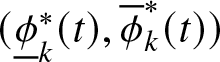 $(\underline{\phi}_{k}^{*}(t),\overline{\phi}_{k}^{*}(t))$ of insurer $k$ are
 \begin{equation}
\left\{
\begin{aligned}
&\underline{\phi}_{k1}^{*}(t)=-\beta_{k1}\xi^{*}_{k}(t)\beta \exp((A_{k}+\vartheta_{k})(T-t)),\\
&\underline{\phi}_{k3}^{*}(t)=1-\exp(\beta_{k3}(\exp((A_{k}+\vartheta_{k})(T-t))q^{*}_{k}(t)y_{k}+\frac{\gamma_k}{2}\exp(2(A_{k}+\vartheta_{k})(T-t))(q^{*}_{k}(t))^{2}y^{2}_{k})),\\
&\underline{\phi}_{k4}^{*}(t)=1-\exp(\beta_{k4}(\exp((A_{k}+\vartheta_{k})(T-t))q^{*}_{k}(t)y_{k}+\frac{\gamma_k}{2}\exp(2(A_{k}+\vartheta_{k})(T-t))(q^{*}_{k}(t))^{2}y^{2}_{k})),
\end{aligned}
\right.
\end{equation}
\begin{equation}
\left\{
\begin{aligned}
&\underline{\phi}_{k1}^{*}(t)=-\beta_{k1}\xi^{*}_{k}(t)\beta \exp((A_{k}+\vartheta_{k})(T-t)),\\
&\underline{\phi}_{k3}^{*}(t)=1-\exp(\beta_{k3}(\exp((A_{k}+\vartheta_{k})(T-t))q^{*}_{k}(t)y_{k}+\frac{\gamma_k}{2}\exp(2(A_{k}+\vartheta_{k})(T-t))(q^{*}_{k}(t))^{2}y^{2}_{k})),\\
&\underline{\phi}_{k4}^{*}(t)=1-\exp(\beta_{k4}(\exp((A_{k}+\vartheta_{k})(T-t))q^{*}_{k}(t)y_{k}+\frac{\gamma_k}{2}\exp(2(A_{k}+\vartheta_{k})(T-t))(q^{*}_{k}(t))^{2}y^{2}_{k})),
\end{aligned}
\right.
\end{equation}and
 \begin{equation}
\left\{
\begin{aligned}
&\overline{\phi}_{k1}^{*}(t)=\beta_{k1}\xi^{*}_{k}(t)\beta \exp((A_{k}+\vartheta_{k})(T-t)),\\
&\overline{\phi}_{k3}^{*}(t)=1-\exp(-\beta_{k3}(\exp((A_{k}+\vartheta_{k})(T-t))q^{*}_{k}(t)y_{k}+\frac{\gamma_k}{2}\exp(2(A_{k}+\vartheta_{k})(T-t))(q^{*}_{k}(t))^{2}y^{2}_{k})),\\
&\overline{\phi}_{k4}^{*}(t)=1-\exp(-\beta_{k4}(\exp((A_{k}+\vartheta_{k})(T-t))q^{*}_{k}(t)y_{k}+\frac{\gamma_k}{2}\exp(2(A_{k}+\vartheta_{k})(T-t))(q^{*}_{k}(t))^{2}y^{2}_{k})).
\end{aligned}
\right.
\end{equation}
\begin{equation}
\left\{
\begin{aligned}
&\overline{\phi}_{k1}^{*}(t)=\beta_{k1}\xi^{*}_{k}(t)\beta \exp((A_{k}+\vartheta_{k})(T-t)),\\
&\overline{\phi}_{k3}^{*}(t)=1-\exp(-\beta_{k3}(\exp((A_{k}+\vartheta_{k})(T-t))q^{*}_{k}(t)y_{k}+\frac{\gamma_k}{2}\exp(2(A_{k}+\vartheta_{k})(T-t))(q^{*}_{k}(t))^{2}y^{2}_{k})),\\
&\overline{\phi}_{k4}^{*}(t)=1-\exp(-\beta_{k4}(\exp((A_{k}+\vartheta_{k})(T-t))q^{*}_{k}(t)y_{k}+\frac{\gamma_k}{2}\exp(2(A_{k}+\vartheta_{k})(T-t))(q^{*}_{k}(t))^{2}y^{2}_{k})).
\end{aligned}
\right.
\end{equation}4.1.2. Solution to non-zero-sum game before default(
$h=0$)

In this subsection, we solve the non-zero-sum stochastic differential reinsurance-investment game before default and provide explicit expressions for the pre-default equilibrium strategy and associated value functions.
Theorem 4.3 (Pre-default)
Consider the  $\alpha$-robust game between two ambiguity-averse insurers with mean-variance utility described in Problem 1. For any $t\in[0,T\wedge\tau]$, the time-consistent Nash equilibrium strategy of insurer $k$, for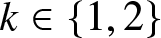 $k\in\{1,2\}$, can be described as follows:
The non-zero-sum differential game investment strategy for corporate bounds is given by
 \begin{equation}
\begin{aligned}
\omega^{*}_{k}(t)&=\frac{[\eta-2\zeta\alpha_{k}h^{p}\exp(\beta_{k2}Y^{*}_{k}-1)+2\zeta\hat{\alpha}_{k}h^{p}\exp(-\beta_{k2}Y^{*}_{k}-1)]E_{k}(t)}{2\hat{\alpha}_{k}h^{p}\exp(-\beta_{k2}Y^{*}_{k}-1)\gamma_{k}\underline{e}^{2}_{k}(t)-2\alpha_{k}h^{p}\exp(\beta_{k2}Y^{*}_{k}-1)\gamma_{k}\overline{e}^{2}_{k}(t)}+n_{k}\omega^{*}_{l}.\\
\end{aligned}
\end{equation}
\begin{equation}
\begin{aligned}
\omega^{*}_{k}(t)&=\frac{[\eta-2\zeta\alpha_{k}h^{p}\exp(\beta_{k2}Y^{*}_{k}-1)+2\zeta\hat{\alpha}_{k}h^{p}\exp(-\beta_{k2}Y^{*}_{k}-1)]E_{k}(t)}{2\hat{\alpha}_{k}h^{p}\exp(-\beta_{k2}Y^{*}_{k}-1)\gamma_{k}\underline{e}^{2}_{k}(t)-2\alpha_{k}h^{p}\exp(\beta_{k2}Y^{*}_{k}-1)\gamma_{k}\overline{e}^{2}_{k}(t)}+n_{k}\omega^{*}_{l}.\\
\end{aligned}
\end{equation} The reinsurance strategy  $q^{*}_{k}(t)$ and the equilibrium investment strategy $\xi^{*}_{k}(t)$ are defined by (4.9) and (4.9), respectively. Additionally, the equilibrium value function of insurer $k$ is given by:
 \begin{equation}
V_{k}(t,\hat{x}_{k},y_{k},y_{l},h)=(\hat{x}_{k}+\vartheta_{k}y_{k}-n_{k}\vartheta_{l}y_{l})\exp((A_{k}+\vartheta_{k})(T-t))+F_{k}(t)s^{-2\varrho}+H_{k}(t)+G_{k1}(t),
\end{equation}
\begin{equation}
V_{k}(t,\hat{x}_{k},y_{k},y_{l},h)=(\hat{x}_{k}+\vartheta_{k}y_{k}-n_{k}\vartheta_{l}y_{l})\exp((A_{k}+\vartheta_{k})(T-t))+F_{k}(t)s^{-2\varrho}+H_{k}(t)+G_{k1}(t),
\end{equation}where  $k\neq l\in\{1,2\}$, $H_{k}(t)$ is defined in (4.14), and
 \begin{equation}
\begin{aligned}
&\frac{\partial F_{k}(t)}{\partial t}+(\overline{D^{\pi_{k}}_{kl}(t)}-n_k\overline{D^{\pi_{l}}_{lk}(t)})\alpha E_{k}(t)-n_k(\hat{\alpha}_{k}-\alpha_{k})\overline{D^{\pi_{l}}_{lk}(t)}^{2}\beta^{2}E_{l}(t) E_{k}(t)\\
&-\frac{\gamma}{2}(\overline{D^{\pi_{k}}_{kl}(t)}-n_k\overline{D^{\pi_{l}}_{lk}(t)})^{2}\beta^2(\alpha_{k}\underline{e^{2}_{k}}(t)+\hat{\alpha}_{k}\overline{e^{2}_{k}}(t))+\frac{(\hat{\alpha_{k}}-\alpha_{k})}{2}\beta_{k1}\beta^{2}\overline{D^{\pi_{k}}_{kl}(t)}E^{2}_{k}(t)=0,~~~~~~~~F_{k}(T)=0\\
\end{aligned}
\end{equation}
\begin{equation}
\begin{aligned}
&\frac{\partial F_{k}(t)}{\partial t}+(\overline{D^{\pi_{k}}_{kl}(t)}-n_k\overline{D^{\pi_{l}}_{lk}(t)})\alpha E_{k}(t)-n_k(\hat{\alpha}_{k}-\alpha_{k})\overline{D^{\pi_{l}}_{lk}(t)}^{2}\beta^{2}E_{l}(t) E_{k}(t)\\
&-\frac{\gamma}{2}(\overline{D^{\pi_{k}}_{kl}(t)}-n_k\overline{D^{\pi_{l}}_{lk}(t)})^{2}\beta^2(\alpha_{k}\underline{e^{2}_{k}}(t)+\hat{\alpha}_{k}\overline{e^{2}_{k}}(t))+\frac{(\hat{\alpha_{k}}-\alpha_{k})}{2}\beta_{k1}\beta^{2}\overline{D^{\pi_{k}}_{kl}(t)}E^{2}_{k}(t)=0,~~~~~~~~F_{k}(T)=0\\
\end{aligned}
\end{equation}. Additionally,
 \begin{equation}
\begin{aligned}
G_{k1}(t)&=\int^{T}_{t}\bigg{[}\frac{\eta[\eta-2\zeta\alpha_{k}h^{p}\exp(\beta_{k2}Y^{*}_{k}-1)+2\zeta\hat{\alpha}_{k}h^{p}\exp(-\beta_{k2}Y^{*}_{k}-1)]}{2\hat{\alpha}_{k}h^{p}\exp(-\beta_{k2}Y^{*}_{k}-1)\gamma_{k}-2\alpha_{k}h^{p}\exp(\beta_{k2}Y^{*}_{k}-1)\gamma_{k}}\\
&+\alpha_{k}h^{p}\frac{1-2\exp(\beta_{k2}Y^{*}_{k}-1)}{\beta_{k2}}+\hat{\alpha}_{k}h^{p}\frac{1-2\exp(-\beta_{k2}Y^{*}_{k}-1)}{\beta_{k2}}\bigg{]}ds.\\
\end{aligned}
\end{equation}
\begin{equation}
\begin{aligned}
G_{k1}(t)&=\int^{T}_{t}\bigg{[}\frac{\eta[\eta-2\zeta\alpha_{k}h^{p}\exp(\beta_{k2}Y^{*}_{k}-1)+2\zeta\hat{\alpha}_{k}h^{p}\exp(-\beta_{k2}Y^{*}_{k}-1)]}{2\hat{\alpha}_{k}h^{p}\exp(-\beta_{k2}Y^{*}_{k}-1)\gamma_{k}-2\alpha_{k}h^{p}\exp(\beta_{k2}Y^{*}_{k}-1)\gamma_{k}}\\
&+\alpha_{k}h^{p}\frac{1-2\exp(\beta_{k2}Y^{*}_{k}-1)}{\beta_{k2}}+\hat{\alpha}_{k}h^{p}\frac{1-2\exp(-\beta_{k2}Y^{*}_{k}-1)}{\beta_{k2}}\bigg{]}ds.\\
\end{aligned}
\end{equation} The expected value of each insurer’s relative surplus at terminal wealth under the probability measure  $\mathrm{Q}^{\underline{\phi}^{*}_{k}}$ is given by
 \begin{equation}
\underline{g}_{k}(t,\hat{x}_{k},y_{k},y_{l},h)=(\hat{x}_{k}+\vartheta_{k}y_{k}-n_{k}\vartheta_{l}y_{l})\exp((A_{k}+\vartheta_{k})(T-t))+\underline{f}_{k}(t)s^{-2\varrho}+\underline{h}_{k}(t)+\underline{G}_{k2}(t),
\end{equation}
\begin{equation}
\underline{g}_{k}(t,\hat{x}_{k},y_{k},y_{l},h)=(\hat{x}_{k}+\vartheta_{k}y_{k}-n_{k}\vartheta_{l}y_{l})\exp((A_{k}+\vartheta_{k})(T-t))+\underline{f}_{k}(t)s^{-2\varrho}+\underline{h}_{k}(t)+\underline{G}_{k2}(t),
\end{equation}where  $k\neq l\in\{1,2\}$, and $\underline{h}_{k}(t)$ is defined in (4.18), and
 \begin{equation}
\begin{aligned}
\underline{f_{k}(t)}&=\exp(-(2\varrho(\alpha+r)-\varrho(2\varrho+1)\beta^{2})(T-t))\int^{T}_{t}[(\underline{D^{\pi_{k}}_{kl}(s)}-n_k\underline{D^{\pi_{l}}_{lk}(s)})\alpha\\
&+(n_k\beta_{l1}\underline{D^{\pi_{l}}_{lk}(s)}-\beta_{k1}\underline{D^{\pi_{k}}_{kl}(s)})]\beta^{2}\exp(2(A_{k}+\vartheta_{k})(T-s))ds
\end{aligned}
\end{equation}
\begin{equation}
\begin{aligned}
\underline{f_{k}(t)}&=\exp(-(2\varrho(\alpha+r)-\varrho(2\varrho+1)\beta^{2})(T-t))\int^{T}_{t}[(\underline{D^{\pi_{k}}_{kl}(s)}-n_k\underline{D^{\pi_{l}}_{lk}(s)})\alpha\\
&+(n_k\beta_{l1}\underline{D^{\pi_{l}}_{lk}(s)}-\beta_{k1}\underline{D^{\pi_{k}}_{kl}(s)})]\beta^{2}\exp(2(A_{k}+\vartheta_{k})(T-s))ds
\end{aligned}
\end{equation}Additionally,
 \begin{equation}
\begin{aligned}
\underline{G}_{k2}(t)&=\int^{T}_{t}\bigg{[}\frac{\eta[\eta-2\zeta\alpha_{k}h^{p}\exp(\beta_{k2}\underline{Y}^{*}_{k}-1)+2\zeta\hat{\alpha}_{k}h^{p}\exp(-\beta_{k2}\underline{Y}^{*}_{k}-1)]}{2\hat{\alpha}_{k}h^{p}\exp(-\beta_{k2}\underline{Y}^{*}_{k}-1)\gamma_{k}-2\alpha_{k}h^{p}\exp(\beta_{k2}\underline{Y}^{*}_{k}-1)\gamma_{k}}\\
&+\exp(\beta_{k2}\underline{Y}^{*}_{k}-1)\frac{h^{p}[\eta-2\zeta\alpha_{k}h^{p}\exp(\beta_{k2}\underline{Y}^{*}_{k}-1)+2\zeta\hat{\alpha}_{k}h^{p}\exp(-\beta_{k2}\underline{Y}^{*}_{k}-1)]E_{k}(s)}{2\hat{\alpha}_{k}h^{p}\exp(-\beta_{k2}\underline{Y}^{*}_{k}-1)\gamma_{k}\underline{e}^{2}_{k}(s)-2\alpha_{k}h^{p}\exp(\beta_{k2}\underline{Y}^{*}_{k}-1)\gamma_{k}\overline{e}^{2}_{k}(s)}\bigg{]}ds\\
\end{aligned}
\end{equation}
\begin{equation}
\begin{aligned}
\underline{G}_{k2}(t)&=\int^{T}_{t}\bigg{[}\frac{\eta[\eta-2\zeta\alpha_{k}h^{p}\exp(\beta_{k2}\underline{Y}^{*}_{k}-1)+2\zeta\hat{\alpha}_{k}h^{p}\exp(-\beta_{k2}\underline{Y}^{*}_{k}-1)]}{2\hat{\alpha}_{k}h^{p}\exp(-\beta_{k2}\underline{Y}^{*}_{k}-1)\gamma_{k}-2\alpha_{k}h^{p}\exp(\beta_{k2}\underline{Y}^{*}_{k}-1)\gamma_{k}}\\
&+\exp(\beta_{k2}\underline{Y}^{*}_{k}-1)\frac{h^{p}[\eta-2\zeta\alpha_{k}h^{p}\exp(\beta_{k2}\underline{Y}^{*}_{k}-1)+2\zeta\hat{\alpha}_{k}h^{p}\exp(-\beta_{k2}\underline{Y}^{*}_{k}-1)]E_{k}(s)}{2\hat{\alpha}_{k}h^{p}\exp(-\beta_{k2}\underline{Y}^{*}_{k}-1)\gamma_{k}\underline{e}^{2}_{k}(s)-2\alpha_{k}h^{p}\exp(\beta_{k2}\underline{Y}^{*}_{k}-1)\gamma_{k}\overline{e}^{2}_{k}(s)}\bigg{]}ds\\
\end{aligned}
\end{equation} The expected value of each insurer’s relative surplus at terminal wealth under the probability measure  $\mathrm{Q}^{\overline{\phi}^{*}_{k}}$ is given by
 \begin{equation}
\overline{g}_{k}(t,\hat{x}_{k},y_{k},y_{l},h)=(\hat{x}_{k}+\vartheta_{k}y_{k}-n_{k}\vartheta_{l}y_{l})\exp((A_{k}+\vartheta_{k})(T-t))+\overline{f}_{k}(t)s^{-2\varrho}+\overline{h}_{k}(t)+\overline{G}_{k2}(t),
\end{equation}
\begin{equation}
\overline{g}_{k}(t,\hat{x}_{k},y_{k},y_{l},h)=(\hat{x}_{k}+\vartheta_{k}y_{k}-n_{k}\vartheta_{l}y_{l})\exp((A_{k}+\vartheta_{k})(T-t))+\overline{f}_{k}(t)s^{-2\varrho}+\overline{h}_{k}(t)+\overline{G}_{k2}(t),
\end{equation}where  $k\neq l\in\{1,2\}$, and $\overline{h}_{k}(t)$ is defined in (4.20), and
 \begin{equation}
\begin{aligned}
\overline{f_{k}}(t)&=\exp(-(2\varrho(\alpha+r)-\varrho(2\varrho+1)\beta^{2})(T-t))\int^{T}_{t}[(\overline{D^{\pi_{k}}_{kl}(s)}-n_k\overline{D^{\pi_{l}}_{lk}(s)})\alpha\\
&+(n_k\beta_{l1}\overline{D^{\pi_{l}}_{lk}(s)}-\beta_{k1}\overline{D^{\pi_{k}}_{kl}(s)})]\beta^{2}\exp(2(A_{k}+\vartheta_{k})(T-s))ds,
\end{aligned}
\end{equation}
\begin{equation}
\begin{aligned}
\overline{f_{k}}(t)&=\exp(-(2\varrho(\alpha+r)-\varrho(2\varrho+1)\beta^{2})(T-t))\int^{T}_{t}[(\overline{D^{\pi_{k}}_{kl}(s)}-n_k\overline{D^{\pi_{l}}_{lk}(s)})\alpha\\
&+(n_k\beta_{l1}\overline{D^{\pi_{l}}_{lk}(s)}-\beta_{k1}\overline{D^{\pi_{k}}_{kl}(s)})]\beta^{2}\exp(2(A_{k}+\vartheta_{k})(T-s))ds,
\end{aligned}
\end{equation}Additionally,
 \begin{equation}
\begin{aligned}
\overline{G_{k2}}(t)&=\int^{T}_{t}\bigg{[}\frac{\eta[\eta-2\zeta\alpha_{k}h^{p}\exp(\beta_{k2}\overline{Y}^{*}_{k}-1)+2\zeta\hat{\alpha}_{k}h^{p}\exp(-\beta_{k2}\overline{Y}^{*}_{k}-1)]}{2\hat{\alpha}_{k}h^{p}\exp(-\beta_{k2}\overline{Y}^{*}_{k}-1)\gamma_{k}-2\alpha_{k}h^{p}\exp(\beta_{k2}\overline{Y}^{*}_{k}-1)\gamma_{k}}\\
&+\exp(-\beta_{k2}\overline{Y}^{*}_{k}-1)\frac{h^{p}[\eta-2\zeta\alpha_{k}h^{p}\exp(\beta_{k2}\overline{Y}^{*}_{k}-1)+2\zeta\hat{\alpha}_{k}h^{p}\exp(-\beta_{k2}\overline{Y}^{*}_{k}-1)]E_{k}(s)}{2\hat{\alpha}_{k}h^{p}\exp(-\beta_{k2}\overline{Y}^{*}_{k}-1)\gamma_{k}\underline{e}^{2}_{k}(s)-2\alpha_{k}h^{p}\exp(\beta_{k2}\overline{Y}^{*}_{k}-1)\gamma_{k}\overline{e}^{2}_{k}(s)}\bigg{]}ds
\end{aligned}
\end{equation}
\begin{equation}
\begin{aligned}
\overline{G_{k2}}(t)&=\int^{T}_{t}\bigg{[}\frac{\eta[\eta-2\zeta\alpha_{k}h^{p}\exp(\beta_{k2}\overline{Y}^{*}_{k}-1)+2\zeta\hat{\alpha}_{k}h^{p}\exp(-\beta_{k2}\overline{Y}^{*}_{k}-1)]}{2\hat{\alpha}_{k}h^{p}\exp(-\beta_{k2}\overline{Y}^{*}_{k}-1)\gamma_{k}-2\alpha_{k}h^{p}\exp(\beta_{k2}\overline{Y}^{*}_{k}-1)\gamma_{k}}\\
&+\exp(-\beta_{k2}\overline{Y}^{*}_{k}-1)\frac{h^{p}[\eta-2\zeta\alpha_{k}h^{p}\exp(\beta_{k2}\overline{Y}^{*}_{k}-1)+2\zeta\hat{\alpha}_{k}h^{p}\exp(-\beta_{k2}\overline{Y}^{*}_{k}-1)]E_{k}(s)}{2\hat{\alpha}_{k}h^{p}\exp(-\beta_{k2}\overline{Y}^{*}_{k}-1)\gamma_{k}\underline{e}^{2}_{k}(s)-2\alpha_{k}h^{p}\exp(\beta_{k2}\overline{Y}^{*}_{k}-1)\gamma_{k}\overline{e}^{2}_{k}(s)}\bigg{]}ds
\end{aligned}
\end{equation} Finally, the worst-case density generators 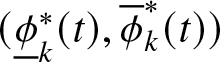 $(\underline{\phi}_{k}^{*}(t),\overline{\phi}_{k}^{*}(t))$ of insurer $k$ are given by
 \begin{equation}
\left\{
\begin{aligned}
&\underline{\phi}_{k1}^{*}(t)=-\beta_{k1}\xi^{*}_{k}(t)\beta \exp((A_{k}+\vartheta_{k})(T-t)),\\
&\underline{\phi}_{k2}^{*}(t)=\exp(\beta_{k2}(\zeta(\omega^{*}_{k}(t)-n_{k}\omega^{*}_{l}(t))E_{k}(t)-\frac{\gamma_{k}}{2}\underline{e}^{2}_{k}(t)\zeta^{2}(\omega^{*}_{k}(t)-n_{k}\omega^{*}_{l}(t))^{2})-1),\\
&\underline{\phi}_{k3}^{*}(t)=1-\exp(\beta_{k3}(\exp((A_{k}+\vartheta_{k})(T-t))q^{*}_{k}(t)y_{k}+\frac{\gamma_k}{2}\exp(2(A_{k}+\vartheta_{k})(T-t))(q^{*}_{k}(t))^{2}y^{2}_{k})),\\
&\underline{\phi}_{k4}^{*}(t)=1-\exp(\beta_{k4}(\exp((A_{k}+\vartheta_{k})(T-t))q^{*}_{k}(t)y_{k}+\frac{\gamma_k}{2}\exp(2(A_{k}+\vartheta_{k})(T-t))(q^{*}_{k}(t))^{2}y^{2}_{k})),
\end{aligned}
\right.
\end{equation}
\begin{equation}
\left\{
\begin{aligned}
&\underline{\phi}_{k1}^{*}(t)=-\beta_{k1}\xi^{*}_{k}(t)\beta \exp((A_{k}+\vartheta_{k})(T-t)),\\
&\underline{\phi}_{k2}^{*}(t)=\exp(\beta_{k2}(\zeta(\omega^{*}_{k}(t)-n_{k}\omega^{*}_{l}(t))E_{k}(t)-\frac{\gamma_{k}}{2}\underline{e}^{2}_{k}(t)\zeta^{2}(\omega^{*}_{k}(t)-n_{k}\omega^{*}_{l}(t))^{2})-1),\\
&\underline{\phi}_{k3}^{*}(t)=1-\exp(\beta_{k3}(\exp((A_{k}+\vartheta_{k})(T-t))q^{*}_{k}(t)y_{k}+\frac{\gamma_k}{2}\exp(2(A_{k}+\vartheta_{k})(T-t))(q^{*}_{k}(t))^{2}y^{2}_{k})),\\
&\underline{\phi}_{k4}^{*}(t)=1-\exp(\beta_{k4}(\exp((A_{k}+\vartheta_{k})(T-t))q^{*}_{k}(t)y_{k}+\frac{\gamma_k}{2}\exp(2(A_{k}+\vartheta_{k})(T-t))(q^{*}_{k}(t))^{2}y^{2}_{k})),
\end{aligned}
\right.
\end{equation}and
 \begin{equation}
\left\{
\begin{aligned}
&\overline{\phi}_{k1}^{*}(t)=\beta_{k1}\xi^{*}_{k}(t)\beta \exp((A_{k}+\vartheta_{k})(T-t)),\\
&\overline{\phi}_{k2}^{*}(t)=\exp(-\beta_{k2}(\zeta(\omega^{*}_{k}(t)-n_{k}\omega^{*}_{l}(t))E_{k}(t)-\frac{\gamma_{k}}{2}\overline{e}^{2}_{k}(t)\zeta^{2}(\omega^{*}_{k}(t)-n_{k}\omega^{*}_{l}(t))^{2})-1),\\
&\overline{\phi}_{k3}^{*}(t)=1-\exp(-\beta_{k3}(\exp((A_{k}+\vartheta_{k})(T-t))q^{*}_{k}(t)y_{k}+\frac{\gamma_k}{2}\exp(2(A_{k}+\vartheta_{k})(T-t))(q^{*}_{k}(t))^{2}y^{2}_{k})),\\
&\overline{\phi}_{k4}^{*}(t)=1-\exp(-\beta_{k4}(\exp((A_{k}+\vartheta_{k})(T-t))q^{*}_{k}(t)y_{k}+\frac{\gamma_k}{2}\exp(2(A_{k}+\vartheta_{k})(T-t))(q^{*}_{k}(t))^{2}y^{2}_{k})).
\end{aligned}
\right.
\end{equation}
\begin{equation}
\left\{
\begin{aligned}
&\overline{\phi}_{k1}^{*}(t)=\beta_{k1}\xi^{*}_{k}(t)\beta \exp((A_{k}+\vartheta_{k})(T-t)),\\
&\overline{\phi}_{k2}^{*}(t)=\exp(-\beta_{k2}(\zeta(\omega^{*}_{k}(t)-n_{k}\omega^{*}_{l}(t))E_{k}(t)-\frac{\gamma_{k}}{2}\overline{e}^{2}_{k}(t)\zeta^{2}(\omega^{*}_{k}(t)-n_{k}\omega^{*}_{l}(t))^{2})-1),\\
&\overline{\phi}_{k3}^{*}(t)=1-\exp(-\beta_{k3}(\exp((A_{k}+\vartheta_{k})(T-t))q^{*}_{k}(t)y_{k}+\frac{\gamma_k}{2}\exp(2(A_{k}+\vartheta_{k})(T-t))(q^{*}_{k}(t))^{2}y^{2}_{k})),\\
&\overline{\phi}_{k4}^{*}(t)=1-\exp(-\beta_{k4}(\exp((A_{k}+\vartheta_{k})(T-t))q^{*}_{k}(t)y_{k}+\frac{\gamma_k}{2}\exp(2(A_{k}+\vartheta_{k})(T-t))(q^{*}_{k}(t))^{2}y^{2}_{k})).
\end{aligned}
\right.
\end{equation}Proof. See Appendix A for specific details of the proof.
Proposition 1. The  $alpha$-robust equilibrium reinsurance strategy $q^{*}_{k}(t)$ of insurer $k$,
$k$,  $k\in\{1,2\}$, can be uniquely determined by equation (4.9). That is, there exists a unique $q^{*}_{k}(t) \gt 0$ satisfying equation (4.9).
Proof. See Appendix B for specific details of the proof.
Proposition 2. For any fixed  $t\in[0,T]$, the equilibrium reinsurance strategy $q_{k}(t)$ is a decreasing function of $\alpha_{k},\beta_{k3},\beta_{k4},\gamma_{k} $.
Proof. See Appendix C for specific details of the proof.
Corollary 3. (1) For an extremely ambiguity-averse insurer  $k$(
$k$( $\alpha_{k}=1$), the equilibrium reinsurance-investment strategy ( $q^{*}_{k}(t),\xi^{*}_{k}(t),\omega^{*}_{k}(t)$) is given by
 \begin{equation*}\qquad\quad
\begin{cases}
&[(\lambda_{k}+\lambda)(\mu_{k}+2\theta_{k}(1-q^{*}_{k})\sigma_{k}^{2})]E_{k}(t)-\int^{\infty}_{0}\exp(\beta_{k3}{X^{*}_{k}})[\beta_{k3}(E_{k}(t)y_{k}+\gamma_{k}{e}^{2}_{k}y^{2}_{k}q^{*}_{k})]\upsilon_{k}(dy_{k}) \nonumber\\
&-\int^{\infty}_{0}\exp(\beta_{k4}{X^{*}_{k}}[\beta_{k4}(E_{k}(t)y_{k}+\gamma_{k}{e}^{2}_{k}y^{2}_{k}q^{*}_{k})]\upsilon(dy_{k})=0, \qquad\qquad\qquad\qquad\qquad\quad\,\,(4.35\textrm{a})\\
&\xi^{*}_{k}=\frac{\frac{E_{k}(t)}{\overline{A_{k}}(t)+\overline{B_{k}}(t)}+\frac{E_{l}(t)}{\overline{A_{l}}(t)+\overline{B_{l}}(t)}\frac{n_{k}\overline{A_{k}}(t)}{\overline{A_{k}}(t)+\overline{B_{k}}(t)}}{1-\frac{n_{k}\overline{A_{k}}(t)}{\overline{A_{k}}(t)+\overline{B_{k}}(t)}\frac{n_{l}\overline{A_{l}}(t)}{\overline{A_{l}}(t)+\overline{B_{l}}(t)}}\triangleq\overline{D^{\pi_{k}}_{kl}}(t), \qquad\qquad\qquad\qquad\qquad\qquad\qquad\qquad\quad\!\!(4.35\textrm{b})\\
&\omega^{*}_{k}(t)=-\frac{[\eta-2\zeta h^{p}\exp(\beta_{k2}Y^{*}_{k}-1)]E_{k}(t)}{2h^{p}\exp(\beta_{k2}Y^{*}_{k}-1)\gamma_{k}{e}^{2}_{k}(t)}+n_{k}\omega^{*}_{l}. \qquad\qquad\quad\qquad\qquad\qquad\qquad\qquad\quad\,\,(4.35\textrm{c})
\end{cases}
\end{equation*}
\begin{equation*}\qquad\quad
\begin{cases}
&[(\lambda_{k}+\lambda)(\mu_{k}+2\theta_{k}(1-q^{*}_{k})\sigma_{k}^{2})]E_{k}(t)-\int^{\infty}_{0}\exp(\beta_{k3}{X^{*}_{k}})[\beta_{k3}(E_{k}(t)y_{k}+\gamma_{k}{e}^{2}_{k}y^{2}_{k}q^{*}_{k})]\upsilon_{k}(dy_{k}) \nonumber\\
&-\int^{\infty}_{0}\exp(\beta_{k4}{X^{*}_{k}}[\beta_{k4}(E_{k}(t)y_{k}+\gamma_{k}{e}^{2}_{k}y^{2}_{k}q^{*}_{k})]\upsilon(dy_{k})=0, \qquad\qquad\qquad\qquad\qquad\quad\,\,(4.35\textrm{a})\\
&\xi^{*}_{k}=\frac{\frac{E_{k}(t)}{\overline{A_{k}}(t)+\overline{B_{k}}(t)}+\frac{E_{l}(t)}{\overline{A_{l}}(t)+\overline{B_{l}}(t)}\frac{n_{k}\overline{A_{k}}(t)}{\overline{A_{k}}(t)+\overline{B_{k}}(t)}}{1-\frac{n_{k}\overline{A_{k}}(t)}{\overline{A_{k}}(t)+\overline{B_{k}}(t)}\frac{n_{l}\overline{A_{l}}(t)}{\overline{A_{l}}(t)+\overline{B_{l}}(t)}}\triangleq\overline{D^{\pi_{k}}_{kl}}(t), \qquad\qquad\qquad\qquad\qquad\qquad\qquad\qquad\quad\!\!(4.35\textrm{b})\\
&\omega^{*}_{k}(t)=-\frac{[\eta-2\zeta h^{p}\exp(\beta_{k2}Y^{*}_{k}-1)]E_{k}(t)}{2h^{p}\exp(\beta_{k2}Y^{*}_{k}-1)\gamma_{k}{e}^{2}_{k}(t)}+n_{k}\omega^{*}_{l}. \qquad\qquad\quad\qquad\qquad\qquad\qquad\qquad\quad\,\,(4.35\textrm{c})
\end{cases}
\end{equation*} (2) For an ambiguity-neutral insurer  $k(\alpha_{k}=\frac{1}{2})$, the equilibrium reinsurance-investment strategy ( $q^{*}_{k}(t),\xi^{*}_{k}(t),\omega^{*}_{k}(t)$) is given by
 \begin{equation*}\qquad\qquad\quad
\begin{cases}
&[(\lambda_{k}+\lambda)(\mu_{k}+2\theta_{k}(1-q^{*}_{k})\sigma_{k}^{2})]E_{k}(t) \nonumber\\
&-\frac{1}{2}\int^{\infty}_{0}(\exp(-\beta_{k3}{X^{*}_{k}})+\exp(\beta_{k3}{X^{*}_{k}}))[\beta_{k3}(E_{k}(t)y_{k}+\gamma_{k}{e}^{2}_{k}y^{2}_{k}q^{*}_{k})]\upsilon_{k}(dy_{k}) \nonumber\\
&-\frac{1}{2}\int^{\infty}_{0}(\exp(-\beta_{k4}{X^{*}_{k}})+\exp(\beta_{k4}{X^{*}_{k}})[\beta_{k4}(E_{k}(t)y_{k}+\gamma_{k}{e}^{2}_{k}y^{2}_{k}q^{*}_{k})]\upsilon(dy_{k})=0, \quad\,\,\,(4.36\textrm{a})\\
&\xi^{*}_{k}(t)=\frac{E_{k}(t)}{\gamma_k\beta^{2}(\underline{e}^{2}_{k}(t)+\overline{e}^{2}_{k})}+\xi^{*}_{l}n_{k}, \ \ \qquad\quad\qquad\qquad\qquad\qquad\qquad\qquad\qquad\qquad(4.36\textrm{b})\\
&\omega^{*}_{k}(t)=\frac{[\eta-\zeta h^{p}\exp(\beta_{k2}Y^{*}_{k}-1)+\zeta h^{p}\exp(-\beta_{k2}Y^{*}_{k}-1)]E_{k}(t)}{h^{p}\exp(-\beta_{k2}Y^{*}_{k}-1)\gamma_{k}\underline{e}^{2}_{k}(t)-h^{p}\exp(\beta_{k2}Y^{*}_{k}-1)\gamma_{k}\overline{e}^{2}_{k}(t)}+n_{k}\omega^{*}_{l}. \quad\qquad\qquad\qquad\,\,\,\,\,{(4.36\textrm{c})}
\end{cases}
\end{equation*}
\begin{equation*}\qquad\qquad\quad
\begin{cases}
&[(\lambda_{k}+\lambda)(\mu_{k}+2\theta_{k}(1-q^{*}_{k})\sigma_{k}^{2})]E_{k}(t) \nonumber\\
&-\frac{1}{2}\int^{\infty}_{0}(\exp(-\beta_{k3}{X^{*}_{k}})+\exp(\beta_{k3}{X^{*}_{k}}))[\beta_{k3}(E_{k}(t)y_{k}+\gamma_{k}{e}^{2}_{k}y^{2}_{k}q^{*}_{k})]\upsilon_{k}(dy_{k}) \nonumber\\
&-\frac{1}{2}\int^{\infty}_{0}(\exp(-\beta_{k4}{X^{*}_{k}})+\exp(\beta_{k4}{X^{*}_{k}})[\beta_{k4}(E_{k}(t)y_{k}+\gamma_{k}{e}^{2}_{k}y^{2}_{k}q^{*}_{k})]\upsilon(dy_{k})=0, \quad\,\,\,(4.36\textrm{a})\\
&\xi^{*}_{k}(t)=\frac{E_{k}(t)}{\gamma_k\beta^{2}(\underline{e}^{2}_{k}(t)+\overline{e}^{2}_{k})}+\xi^{*}_{l}n_{k}, \ \ \qquad\quad\qquad\qquad\qquad\qquad\qquad\qquad\qquad\qquad(4.36\textrm{b})\\
&\omega^{*}_{k}(t)=\frac{[\eta-\zeta h^{p}\exp(\beta_{k2}Y^{*}_{k}-1)+\zeta h^{p}\exp(-\beta_{k2}Y^{*}_{k}-1)]E_{k}(t)}{h^{p}\exp(-\beta_{k2}Y^{*}_{k}-1)\gamma_{k}\underline{e}^{2}_{k}(t)-h^{p}\exp(\beta_{k2}Y^{*}_{k}-1)\gamma_{k}\overline{e}^{2}_{k}(t)}+n_{k}\omega^{*}_{l}. \quad\qquad\qquad\qquad\,\,\,\,\,{(4.36\textrm{c})}
\end{cases}
\end{equation*} (3) In the absence of ambiguity  $(\beta_{k1},\beta_{k2},\beta_{k3},\beta_{k4})\downarrow(0,0,0,0)$, the equilibrium reinsurance-investment strategy ( $q^{*}_{k}(t),\xi^{*}_{k}(t),\omega^{*}_{k}(t)$) is given by
 \begin{equation*}\qquad\quad
\begin{cases}
& q^{*}_{k}(t)=\frac{2\theta_{k}\sigma^{2}_{k}\exp(-(A_{k}+\vartheta_{k})(T-t))}{\gamma_{k}\sigma_{k}+2\theta_{k}\sigma^{2}_{k}\exp(-(A_{k}+\vartheta_{k})(T-t))}, \qquad\quad\quad\qquad\qquad\qquad\qquad\qquad\qquad\qquad{(4.37\textrm{a})}\\
&\xi^{*}_{k}(t)=\frac{\exp(-(A_{k}+\vartheta_{k})(T-t))}{\gamma_k\beta^{2}}+\xi^{*}_{l}n_{k}, \qquad\quad\quad\quad\qquad\qquad\qquad\qquad\qquad\qquad\qquad\,\,{(4.37\textrm{b})}\\
&\omega^{*}_{k}(t)=-\frac{[\eta -2\zeta h^{p}]\exp(-(A_{k}+\vartheta_{k})(T-t))}{2h^{p}\gamma_{k}}+n_{k}\omega^{*}_{l}. \qquad\quad\quad\quad\qquad\qquad\qquad\qquad\qquad\,{(4.37\textrm{c})}
\end{cases}
\end{equation*}
\begin{equation*}\qquad\quad
\begin{cases}
& q^{*}_{k}(t)=\frac{2\theta_{k}\sigma^{2}_{k}\exp(-(A_{k}+\vartheta_{k})(T-t))}{\gamma_{k}\sigma_{k}+2\theta_{k}\sigma^{2}_{k}\exp(-(A_{k}+\vartheta_{k})(T-t))}, \qquad\quad\quad\qquad\qquad\qquad\qquad\qquad\qquad\qquad{(4.37\textrm{a})}\\
&\xi^{*}_{k}(t)=\frac{\exp(-(A_{k}+\vartheta_{k})(T-t))}{\gamma_k\beta^{2}}+\xi^{*}_{l}n_{k}, \qquad\quad\quad\quad\qquad\qquad\qquad\qquad\qquad\qquad\qquad\,\,{(4.37\textrm{b})}\\
&\omega^{*}_{k}(t)=-\frac{[\eta -2\zeta h^{p}]\exp(-(A_{k}+\vartheta_{k})(T-t))}{2h^{p}\gamma_{k}}+n_{k}\omega^{*}_{l}. \qquad\quad\quad\quad\qquad\qquad\qquad\qquad\qquad\,{(4.37\textrm{c})}
\end{cases}
\end{equation*}5. Analysis of the results and numerical illustration
In this section, we support the theoretical part with numerical simulations, with most parameter values referenced from Li et al. [Reference Li, Li and Xiong19]. Suppose that the aggregate insurance claims follow a compound Poisson structure. The dynamics of the insurance surplus process without reinsurance and investment, as given in (2.3), are governed by
 \begin{equation}
U_{k}(t)=u_{k}+d_{k}t-P_{k}(t),
\end{equation}
\begin{equation}
U_{k}(t)=u_{k}+d_{k}t-P_{k}(t),
\end{equation}where the associated Levy measures are given by
 \begin{equation}
\upsilon_{k}(dy_{k})=\upsilon(dy_{k})=\lambda \frac{\frac{1}{\sqrt{2\pi}\sigma_{k}}\exp{-\frac{(y_k-\mu_{k})^2}{2\sigma^2_{k}}}}{1-\Phi(-\frac{\mu_{k}}{\sigma_{k}})}dy_k,
\end{equation}
\begin{equation}
\upsilon_{k}(dy_{k})=\upsilon(dy_{k})=\lambda \frac{\frac{1}{\sqrt{2\pi}\sigma_{k}}\exp{-\frac{(y_k-\mu_{k})^2}{2\sigma^2_{k}}}}{1-\Phi(-\frac{\mu_{k}}{\sigma_{k}})}dy_k,
\end{equation}and  $t=0,$ $T=6$,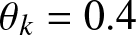 $\theta_{k}=0.4$,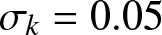 $\sigma_{k}=0.05$, $\gamma_{k}=\gamma_{l}=0.54$, $\lambda_{k}=\lambda_{l}=\lambda=1$,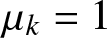 $\mu_{k}=1$, $\beta_{k2}=\beta_{l2}=0.2$,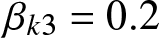 $\beta_{k3}=0.2$,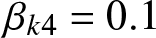 $\beta_{k4}=0.1$, $h_p=0.1$,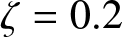 $\zeta=0.2$, $n_k=n_l=0.5$, $A_l=A_k=0.04$Footnote 1, and $\vartheta_l= \vartheta_{k}=0.066$. Since the equation satisfying the optimal reinsurance strategy is implicit, we utilize the “nleqslv” package in R to solve for the optimal reinsurance strategy $q^{*}_{k}$ point-wise, given the risk aversion $\alpha_k$. The difference between $\alpha_k$ and $\alpha_{k+1}$ is 0.0001. Furthermore, to facilitate integration, we set the maximum value of a single claim to 100.
Regarding Figure 1, we observe that the optimal reinsurance strategy decreases with an increase in the ambiguity aversion coefficient. That is, when insurers are more averse to ambiguity (more pessimistic), they transfer the claim risks they bear by paying a certain premium, resulting in a reduction in the optimal reinsurance strategy. Second, the same conclusion can be drawn for  $\gamma_k,~\beta_{k3},~\beta_{k4}$. These numerical simulation results validate the theoretical conclusions presented earlier.
The effect of  $\alpha_k$,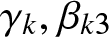 $\gamma_{k}, \beta_{k3}$, and $\beta_{k4}$ on optimal reinsurance strategy.

Table 1 provides deeper insights into how the investment strategies in defaultable bonds ( $\omega^{*}_{k}$ and $\omega^{*}_{l}$) are influenced by the ambiguity aversion levels of both the insurer ( $\alpha_k$) and the competitor ( $\alpha_l$). We report the results in four panels to isolate the effects of the parameters. The following distinct phenomena can be observed:
The effect of  $\alpha_k$ and $\alpha_l$ on corporate bound investment strategy.

First, by comparing Panels B, C, and D vertically, we find that for a fixed level of the competitor’s ambiguity aversion  $\alpha_l$, a higher $\alpha_k$ leads to a lower optimal investment $\omega^{*}_{k}$. This confirms the **direct effect** of ambiguity aversion: as the insurer becomes more pessimistic about the market model (higher $\alpha_k$), they adopt a more conservative strategy by reducing their exposure to risky corporate bonds.
Second, and more interestingly, the horizontal comparison within Panels B, C, and D reveals a strategic interaction effect. When we fix the insurer’s own parameter  $\alpha_k$ (e.g., in Panel B, $\alpha_k=0.596$), as the competitor becomes less ambiguity-averse (i.e., $\alpha_l$ decreases from 0.601 to 0.596), the competitor increases their risky investment $\omega^{*}_{l}$ (from 1.386 to 1.567). Crucially, the insurer $k$ responds by increasing their own investment $\omega^{*}_{k}$ (from 4.634 to 4.729), despite their own preference $\alpha_k$ remaining constant.
This result suggests that the investment strategies are strategic complements. Due to the relative performance concern (competition mechanism), if the competitor adopts an aggressive investment stance driven by lower ambiguity aversion, the insurer  $k$ is compelled to increase their risk exposure to prevent falling behind in relative wealth. Conversely, if the competitor retreats due to high pessimism, the insurer $k$ also reduces their position. Panel A shows the combined effect: when $\alpha_k$ increases and $\alpha_l$ decreases simultaneously, the direct effect of $\alpha_k$ dominates, causing $\omega^{*}_{k}$ to decrease overall, but the presence of competition mitigates the magnitude of this reduction compared to a non-game setting.
6. Conclusion
In this study, we investigated a non-zero-sum differential alpha-robust investment and reinsurance problem between two competitive insurers within a time-consistent mean-variance framework, drawing inspiration from the work of Li et al. [Reference Li, Li and Xiong19]. We assumed that the claim arrival processes for both insurers follow the classical Cramér–Lundberg model, with reinsurance premiums calculated using the variance premium principle. The investment opportunities available to the insurers include a risk-free asset, a risky asset, and a defaultable corporate bond. Our analysis also incorporates the impact of bounded memory, represented by a wealth process with delays. The objective of each insurer is to maximize the expected terminal wealth with delay relative to their competitors while also minimizing the variance of the terminal wealth with delay, amid varying degrees of ambiguity aversion. By employing the game-theoretic framework, we derived the non-zero-sum differential alpha-robust equilibrium strategies and the associated value functions by solving the extended HJB equations. In the conclusions drawn from our numerical simulations, we identified a notable trend: the optimal investment strategy in defaultable bonds diminishes with an increase in a competitor’s risk aversion coefficient, assuming one’s own risk aversion coefficient is unchanged. Intriguingly, this investment strategy’s optimal level continues to decrease with an increase in one’s own risk aversion coefficient, even when a competitor’s risk aversion coefficient moves in an opposing direction. This underscores the nuanced interplay between an insurer’s risk preferences and the competitive market dynamics, which shape the investment strategies in the presence of default risk. In the future, we might investigate scenarios where the risk aversion parameters follow a distribution of a random variable, bringing our model closer to real-world conditions.
Disclosure of interest
The authors declare that they have no potential competing interest to disclose regarding the content of this article.
Conflict of interest
The authors declare that they have no potential competing interest to disclose regarding the content of this article.
Appendix A
Proof. When  $H(t)=0$, the extended HJB system of equations (4.3) and (4.5) becomes:
 \begin{equation*}\qquad\quad
\begin{cases}
&\sup\limits_{\pi_{k}\in\Pi_{k}}\{\alpha\inf_{\phi_{k\in\Phi_{k}}}[\mathcal{L}^{\pi,Q^{\phi_{k}}}V(t,\hat{x}_{k},s,y_{k},y_{l},0)-\frac{\gamma}{2}\mathcal{L}^{\pi,Q^{\phi_{k}}}\underline{g}^{2}(t,\hat{x}_{k},s,y_{k},y_{l},0)\nonumber\\
&+\gamma \underline{g}(t,\hat{x}_{k},s,y_{k},y_{l},0)\mathcal{L}^{\pi,Q^{\phi_{k}}}\underline{g}(t,\hat{x}_{k},s,y_{k},y_{l},0)+h_{\beta}(\phi_{k})]\nonumber\\
&+\hat{\alpha}\sup_{\phi_{k\in\Phi_{k}}}[\mathcal{L}^{\pi,Q^{\phi_{k}}}(t,\hat{x}_{k},s,y_{k},y_{l},0)-\frac{\gamma}{2}\mathcal{L}^{\pi,Q^{\phi_{k}}}\overline{g}^{2}(t,\hat{x}_{k},s,y_{k},y_{l},0)\nonumber\\
+\gamma &\overline{g}(t,\hat{x}_{k},s,y_{k},y_{l},0)\mathcal{L}^{\pi,Q^{\phi_{k}}}\overline{g}(t,\hat{x}_{k},s,y_{k},y_{l},0)+h_{\beta}(\phi_{k})]\}=0 \qquad\qquad\qquad\quad\quad\text{(A.1a)}\\
&V(T,\hat{x}_{k},s,y_{k},y_{l},0)=\hat{x}_{k}+\vartheta_{k}y_{k}-n_{k}\vartheta_{l}y_{l}, \quad\qquad\qquad\qquad\qquad\qquad\qquad\qquad\text{(A.1b)}\\
&\mathcal{L}^{\pi^{*}_{k},Q^{\underline{\phi}_{k}}}\underline{g}(t,\hat{x}_{k},s,y_{k},y_{l},0)=0, \ \qquad\qquad\qquad\qquad\qquad\qquad\qquad\qquad\qquad\quad\text{(A.1c)}\\
&\underline{g}(T,\hat{x}_{k},s,y_{k},y_{l},0)=\hat{x}_{k}+\vartheta_{k}y_{k}-n_{k}\vartheta_{l}y_{l}, \ \qquad\qquad\qquad\qquad\qquad\qquad\qquad\quad\text{(A.1d)}\\
&\mathcal{L}^{\pi^{*}_{k},Q^{\overline{\phi}_{k}}}\overline{g}(t,\hat{x}_{k},s,y_{k},y_{l},0)=0, \ \qquad\qquad\qquad\qquad\qquad\qquad\qquad\qquad\qquad\quad\text{(A.1e)}\\
&\overline{g}(T,\hat{x}_{k},s,y_{k},y_{l},0)=\hat{x}_{k}+\vartheta_{k}y_{k}-n_{k}\vartheta_{l}y_{l}, \ \qquad\qquad\qquad\qquad\qquad\qquad\qquad\quad\text{(A.1f)}
\end{cases}
\end{equation*}
\begin{equation*}\qquad\quad
\begin{cases}
&\sup\limits_{\pi_{k}\in\Pi_{k}}\{\alpha\inf_{\phi_{k\in\Phi_{k}}}[\mathcal{L}^{\pi,Q^{\phi_{k}}}V(t,\hat{x}_{k},s,y_{k},y_{l},0)-\frac{\gamma}{2}\mathcal{L}^{\pi,Q^{\phi_{k}}}\underline{g}^{2}(t,\hat{x}_{k},s,y_{k},y_{l},0)\nonumber\\
&+\gamma \underline{g}(t,\hat{x}_{k},s,y_{k},y_{l},0)\mathcal{L}^{\pi,Q^{\phi_{k}}}\underline{g}(t,\hat{x}_{k},s,y_{k},y_{l},0)+h_{\beta}(\phi_{k})]\nonumber\\
&+\hat{\alpha}\sup_{\phi_{k\in\Phi_{k}}}[\mathcal{L}^{\pi,Q^{\phi_{k}}}(t,\hat{x}_{k},s,y_{k},y_{l},0)-\frac{\gamma}{2}\mathcal{L}^{\pi,Q^{\phi_{k}}}\overline{g}^{2}(t,\hat{x}_{k},s,y_{k},y_{l},0)\nonumber\\
+\gamma &\overline{g}(t,\hat{x}_{k},s,y_{k},y_{l},0)\mathcal{L}^{\pi,Q^{\phi_{k}}}\overline{g}(t,\hat{x}_{k},s,y_{k},y_{l},0)+h_{\beta}(\phi_{k})]\}=0 \qquad\qquad\qquad\quad\quad\text{(A.1a)}\\
&V(T,\hat{x}_{k},s,y_{k},y_{l},0)=\hat{x}_{k}+\vartheta_{k}y_{k}-n_{k}\vartheta_{l}y_{l}, \quad\qquad\qquad\qquad\qquad\qquad\qquad\qquad\text{(A.1b)}\\
&\mathcal{L}^{\pi^{*}_{k},Q^{\underline{\phi}_{k}}}\underline{g}(t,\hat{x}_{k},s,y_{k},y_{l},0)=0, \ \qquad\qquad\qquad\qquad\qquad\qquad\qquad\qquad\qquad\quad\text{(A.1c)}\\
&\underline{g}(T,\hat{x}_{k},s,y_{k},y_{l},0)=\hat{x}_{k}+\vartheta_{k}y_{k}-n_{k}\vartheta_{l}y_{l}, \ \qquad\qquad\qquad\qquad\qquad\qquad\qquad\quad\text{(A.1d)}\\
&\mathcal{L}^{\pi^{*}_{k},Q^{\overline{\phi}_{k}}}\overline{g}(t,\hat{x}_{k},s,y_{k},y_{l},0)=0, \ \qquad\qquad\qquad\qquad\qquad\qquad\qquad\qquad\qquad\quad\text{(A.1e)}\\
&\overline{g}(T,\hat{x}_{k},s,y_{k},y_{l},0)=\hat{x}_{k}+\vartheta_{k}y_{k}-n_{k}\vartheta_{l}y_{l}, \ \qquad\qquad\qquad\qquad\qquad\qquad\qquad\quad\text{(A.1f)}
\end{cases}
\end{equation*}According to the boundary values in (6.1b), (6.2d), and (6.3f), we conjecture that the solutions have the following forms:
 \begin{equation}
\left\{
\begin{aligned}
V(t,\hat{x}_{k},y_{k},y_{l},h)&=E_{k}(t)(\hat{x}_{k}+\vartheta_{k}y_{k}-n_{k}\vartheta_{l}y_{l})+\widetilde{H}_{k}(t),\\
&=E_{k}(t)(\hat{x}_{k}+\vartheta_{k}y_{k}-n_{k}\vartheta_{l}y_{l})+{H}_{k}(t)+G_{k1}(t),\\
\underline{g}(t,\hat{x}_{k},y_{k},y_{l},h)&=\underline{e_{k}}(t)(\hat{x}_{k}+\vartheta_{k}y_{k}-n_{k}\vartheta_{l}y_{l})+\underline{\widetilde{h}}_{k}(t),\\
&=\underline{e_{k}}(t)(\hat{x}_{k}+\vartheta_{k}y_{k}-n_{k}\vartheta_{l}y_{l})+\underline{{h}}_{k}(t)+\underline{G}_{k2}(t),\\
\overline{g}(t,\hat{x}_{k},y_{k},y_{l},h)&=\overline{e_{k}}(t)(\hat{x}_{k}+\vartheta_{k}y_{k}-n_{k}\vartheta_{l}y_{l})+\overline{\widetilde{h}}_{k}(t),\\
&=\overline{e_{k}}(t)(\hat{x}_{k}+\vartheta_{k}y_{k}-n_{k}\vartheta_{l}y_{l})+\overline{{h}}_{k}(t)+\overline{G}_{k2}(t),
\end{aligned}
\right.
\end{equation}
\begin{equation}
\left\{
\begin{aligned}
V(t,\hat{x}_{k},y_{k},y_{l},h)&=E_{k}(t)(\hat{x}_{k}+\vartheta_{k}y_{k}-n_{k}\vartheta_{l}y_{l})+\widetilde{H}_{k}(t),\\
&=E_{k}(t)(\hat{x}_{k}+\vartheta_{k}y_{k}-n_{k}\vartheta_{l}y_{l})+{H}_{k}(t)+G_{k1}(t),\\
\underline{g}(t,\hat{x}_{k},y_{k},y_{l},h)&=\underline{e_{k}}(t)(\hat{x}_{k}+\vartheta_{k}y_{k}-n_{k}\vartheta_{l}y_{l})+\underline{\widetilde{h}}_{k}(t),\\
&=\underline{e_{k}}(t)(\hat{x}_{k}+\vartheta_{k}y_{k}-n_{k}\vartheta_{l}y_{l})+\underline{{h}}_{k}(t)+\underline{G}_{k2}(t),\\
\overline{g}(t,\hat{x}_{k},y_{k},y_{l},h)&=\overline{e_{k}}(t)(\hat{x}_{k}+\vartheta_{k}y_{k}-n_{k}\vartheta_{l}y_{l})+\overline{\widetilde{h}}_{k}(t),\\
&=\overline{e_{k}}(t)(\hat{x}_{k}+\vartheta_{k}y_{k}-n_{k}\vartheta_{l}y_{l})+\overline{{h}}_{k}(t)+\overline{G}_{k2}(t),
\end{aligned}
\right.
\end{equation}where the boundary conditions are given by
 \begin{equation*}E_{k}(T)=\underline{e_{k}}(T)=\overline{e_{k}}(T)=1,~\widetilde{H}_{k}(T)=\underline{\widetilde{h}}_{k}(T)=\overline{\widetilde{h}}_{k}(T)=0.\end{equation*}
 Suppose that  $A_{k}+\upsilon_{k}=A_{l}+\upsilon_{l}$. For convenience, we redefine conformity as follows:
 \begin{equation}
\begin{aligned}
&L(t,\hat{x}_{k},s,y_{k},y_{l},0)\triangleq\\
&[\frac{\partial E_{k}(t)}{\partial t}+(A_{k}+\vartheta_{k})E_{k}(t)](\hat{x}_{k}+\vartheta_{k}y_{k}-n_{k}\vartheta_{l}y_{l})+\frac{\partial F_{k}(t)}{\partial t}s^{-2\varrho}+\frac{\partial H(t)}{\partial t}+\\
&[d_{k}-(\lambda_k+\lambda)(1-q_{k})\mu_k-\theta_k(1-q_{k})^{2}(\lambda_k+\lambda)\sigma^{2}_{k}-n_kd_{l}+n_k(\lambda_l+\lambda)(1-q^{*}_{l})\mu_l+(\omega_{k}(t)-n_{k}\omega_{l}(t))\eta\\
&+n_k\theta_l(1-q^{*}_{l}(t))^{2}(\lambda_l+\lambda)\sigma^{2}_{l}+(\xi_{k}-n_k\xi^{*}_l(t))\alpha-n_k\phi_{l1}\xi^{*}_{l}(t)\beta ]E_{k}(t)-\frac{\gamma}{2}(\xi_{k}-n_k\xi^{*}_l(t))^{2}\beta^2e^{2}_{k}(t)\\
&+\int^{\infty}_{0}(n_{k}E_{k}(t)q_{l}y_{l}-\frac{\gamma_{k}}{2}n^{2}_{k}e^{2}_{k}q^{2}_{l}y^{2}_{l})(1-\phi_{l3}(t,y_{l}))\upsilon_{l}(dy_{l})+\int^{\infty}_{0}(n_{k}E_{k}(t)q_{l}y_{l}-\frac{\gamma_{k}}{2}n^{2}_{k}e^{2}_{k}q^{2}_{l}y^{2}_{l})\\
&\times (1-\phi_{l4}(t,y_{k}))\upsilon(dy_{l}).\\
\end{aligned}
\end{equation}
\begin{equation}
\begin{aligned}
&L(t,\hat{x}_{k},s,y_{k},y_{l},0)\triangleq\\
&[\frac{\partial E_{k}(t)}{\partial t}+(A_{k}+\vartheta_{k})E_{k}(t)](\hat{x}_{k}+\vartheta_{k}y_{k}-n_{k}\vartheta_{l}y_{l})+\frac{\partial F_{k}(t)}{\partial t}s^{-2\varrho}+\frac{\partial H(t)}{\partial t}+\\
&[d_{k}-(\lambda_k+\lambda)(1-q_{k})\mu_k-\theta_k(1-q_{k})^{2}(\lambda_k+\lambda)\sigma^{2}_{k}-n_kd_{l}+n_k(\lambda_l+\lambda)(1-q^{*}_{l})\mu_l+(\omega_{k}(t)-n_{k}\omega_{l}(t))\eta\\
&+n_k\theta_l(1-q^{*}_{l}(t))^{2}(\lambda_l+\lambda)\sigma^{2}_{l}+(\xi_{k}-n_k\xi^{*}_l(t))\alpha-n_k\phi_{l1}\xi^{*}_{l}(t)\beta ]E_{k}(t)-\frac{\gamma}{2}(\xi_{k}-n_k\xi^{*}_l(t))^{2}\beta^2e^{2}_{k}(t)\\
&+\int^{\infty}_{0}(n_{k}E_{k}(t)q_{l}y_{l}-\frac{\gamma_{k}}{2}n^{2}_{k}e^{2}_{k}q^{2}_{l}y^{2}_{l})(1-\phi_{l3}(t,y_{l}))\upsilon_{l}(dy_{l})+\int^{\infty}_{0}(n_{k}E_{k}(t)q_{l}y_{l}-\frac{\gamma_{k}}{2}n^{2}_{k}e^{2}_{k}q^{2}_{l}y^{2}_{l})\\
&\times (1-\phi_{l4}(t,y_{k}))\upsilon(dy_{l}).\\
\end{aligned}
\end{equation}By relating (4.2), (4.3), and (4.6) and integrating them with simplification, we obtain the following equation:
 \begin{equation}
\begin{aligned}
&\sup_{\pi_{k}\in\Pi_{k}}\{\alpha_{k}\inf_{\phi_{k}\in\Phi_{k}}\{\underline{L}^{k}(t,\hat{x}_{k},s,y_{k},y_{l},h)+\underline{\phi}_{k1}\xi_{k}\beta E_{k}(t)+\int^{\infty}_{0}(-E_{k}(t)q_{k}y_{k}-\frac{\gamma}{2}\underline{e}^{2}_{k}q^{2}_{k}y^{2}_{k})\\
& \times(1-\underline{\phi}_{k3}(t,y_{k}))\upsilon_{k}(dy_{k})+\int^{\infty}_{0}(-E_{k}(t)q_{k}y_{k}-\frac{\gamma}{2}\underline{e}^{2}_{k}q^{2}_{k}y^{2}_{k})(1-\underline{\phi}_{k4}(t,y_{k}))\upsilon(dy_{k})\\
&+[-\zeta(\omega_{k}(t)-n_{k}\omega_{l}(t))E_{k}(t)-\frac{\gamma_{k}}{2}\underline{e}^{2}_{k}(t)\zeta^{2}(\omega_{k}(t)-n_{k}\omega_{l}(t))^{2}]h^{p}(1-h)\underline{\phi}_{k2}+h_{\beta}(\phi_k)\}\\
&+\hat{\alpha}_{k}\sup_{\phi_{k}\in\Phi_{k}}\{\overline{L}^{k}(t,\hat{x}_{k},s,y_{k},y_{l},h)+\overline{\phi}_{k1}\xi_{k}\beta E_{k}(t)+\int^{\infty}_{0}(-E_{k}(t)q_{k}y_{k}-\frac{\gamma}{2}\overline{e}^{2}_{k}q^{2}_{k}y^{2}_{k})(1-\overline{\phi}_{k3}(t,y_{k}))\upsilon_{k}(dy_{k})\\
&+\int^{\infty}_{0}(-E_{k}(t)q_{k}y_{k}-\frac{\gamma}{2}\overline{e}^{2}_{k}q^{2}_{k}y^{2}_{k})(1-\overline{\phi}_{k4}(t,y_{k}))\upsilon(dy_{k})\\
&+[-\zeta(\omega_{k}(t)-n_{k}\omega_{l}(t))E_{k}(t)-\frac{\gamma_{k}}{2}\overline{e}^{2}_{k}(t)\zeta^{2}(\omega_{k}(t)-n_{k}\omega_{l}(t))^{2}]h^{p}(1-h)\overline{\phi}_{k2}-h_{\beta}(\phi_k)\}\}=0
\end{aligned}
\end{equation}
\begin{equation}
\begin{aligned}
&\sup_{\pi_{k}\in\Pi_{k}}\{\alpha_{k}\inf_{\phi_{k}\in\Phi_{k}}\{\underline{L}^{k}(t,\hat{x}_{k},s,y_{k},y_{l},h)+\underline{\phi}_{k1}\xi_{k}\beta E_{k}(t)+\int^{\infty}_{0}(-E_{k}(t)q_{k}y_{k}-\frac{\gamma}{2}\underline{e}^{2}_{k}q^{2}_{k}y^{2}_{k})\\
& \times(1-\underline{\phi}_{k3}(t,y_{k}))\upsilon_{k}(dy_{k})+\int^{\infty}_{0}(-E_{k}(t)q_{k}y_{k}-\frac{\gamma}{2}\underline{e}^{2}_{k}q^{2}_{k}y^{2}_{k})(1-\underline{\phi}_{k4}(t,y_{k}))\upsilon(dy_{k})\\
&+[-\zeta(\omega_{k}(t)-n_{k}\omega_{l}(t))E_{k}(t)-\frac{\gamma_{k}}{2}\underline{e}^{2}_{k}(t)\zeta^{2}(\omega_{k}(t)-n_{k}\omega_{l}(t))^{2}]h^{p}(1-h)\underline{\phi}_{k2}+h_{\beta}(\phi_k)\}\\
&+\hat{\alpha}_{k}\sup_{\phi_{k}\in\Phi_{k}}\{\overline{L}^{k}(t,\hat{x}_{k},s,y_{k},y_{l},h)+\overline{\phi}_{k1}\xi_{k}\beta E_{k}(t)+\int^{\infty}_{0}(-E_{k}(t)q_{k}y_{k}-\frac{\gamma}{2}\overline{e}^{2}_{k}q^{2}_{k}y^{2}_{k})(1-\overline{\phi}_{k3}(t,y_{k}))\upsilon_{k}(dy_{k})\\
&+\int^{\infty}_{0}(-E_{k}(t)q_{k}y_{k}-\frac{\gamma}{2}\overline{e}^{2}_{k}q^{2}_{k}y^{2}_{k})(1-\overline{\phi}_{k4}(t,y_{k}))\upsilon(dy_{k})\\
&+[-\zeta(\omega_{k}(t)-n_{k}\omega_{l}(t))E_{k}(t)-\frac{\gamma_{k}}{2}\overline{e}^{2}_{k}(t)\zeta^{2}(\omega_{k}(t)-n_{k}\omega_{l}(t))^{2}]h^{p}(1-h)\overline{\phi}_{k2}-h_{\beta}(\phi_k)\}\}=0
\end{aligned}
\end{equation} Applying the Differential Theorem to (4.3), when equation (4.3) reaches its maximum value with respect to  $\phi_k$, we obtain the following equation:
 \begin{equation}
\left\{
\begin{aligned}
&\underline{\phi}_{k1}^{*}(t)=-\beta_{k1}\xi_{k}\beta E_{k}(t),\\
&\underline{\phi}_{k2}^{*}(t)=\exp(\beta_{k2}(\zeta(\omega_{k}(t)-n_{k}\omega_{l}(t))E_{k}(t)-\frac{\gamma_{k}}{2}\underline{e}^{2}_{k}(t)\zeta^{2}(\omega_{k}(t)-n_{k}\omega_{l}(t))^{2})-1),\\
&\underline{\phi}_{k3}^{*}(t)=1-\exp(\beta_{k3}(E_{k}(t)q_{k}y_{k}+\frac{\gamma}{2}\underline{e}^{2}_{k}q^{2}_{k}y^{2}_{k})),\\
&\underline{\phi}_{k4}^{*}(t)=1-\exp(\beta_{k4}(E_{k}(t)q_{k}y_{k}+\frac{\gamma}{2}\underline{e}^{2}_{k}q^{2}_{k}y^{2}_{k})),
\end{aligned}
\right.
\end{equation}
\begin{equation}
\left\{
\begin{aligned}
&\underline{\phi}_{k1}^{*}(t)=-\beta_{k1}\xi_{k}\beta E_{k}(t),\\
&\underline{\phi}_{k2}^{*}(t)=\exp(\beta_{k2}(\zeta(\omega_{k}(t)-n_{k}\omega_{l}(t))E_{k}(t)-\frac{\gamma_{k}}{2}\underline{e}^{2}_{k}(t)\zeta^{2}(\omega_{k}(t)-n_{k}\omega_{l}(t))^{2})-1),\\
&\underline{\phi}_{k3}^{*}(t)=1-\exp(\beta_{k3}(E_{k}(t)q_{k}y_{k}+\frac{\gamma}{2}\underline{e}^{2}_{k}q^{2}_{k}y^{2}_{k})),\\
&\underline{\phi}_{k4}^{*}(t)=1-\exp(\beta_{k4}(E_{k}(t)q_{k}y_{k}+\frac{\gamma}{2}\underline{e}^{2}_{k}q^{2}_{k}y^{2}_{k})),
\end{aligned}
\right.
\end{equation}and
 \begin{equation}
\left\{
\begin{aligned}
&\overline{\phi}_{k1}^{*}(t)=\beta_{k1}\xi_{k}\beta E_{k}(t),\\
&\overline{\phi}_{k2}^{*}(t)=\exp(-\beta_{k2}(\zeta(\omega_{k}(t)-n_{k}\omega_{l}(t))E_{k}(t)-\frac{\gamma_{k}}{2}\overline{e}^{2}_{k}(t)\zeta^{2}(\omega_{k}(t)-n_{k}\omega_{l}(t))^{2})-1),\\
&\overline{\phi}_{k3}^{*}(t)=1-\exp(-\beta_{k3}(E_{k}(t)q_{k}y_{k}+\frac{\gamma}{2}\overline{e}^{2}_{k}q^{2}_{k}y^{2}_{k})),\\
&\overline{\phi}_{k4}^{*}(t)=1-\exp(-\beta_{k4}(E_{k}(t)q_{k}y_{k}+\frac{\gamma}{2}\overline{e}^{2}_{k}q^{2}_{k}y^{2}_{k})).
\end{aligned}
\right.
\end{equation}
\begin{equation}
\left\{
\begin{aligned}
&\overline{\phi}_{k1}^{*}(t)=\beta_{k1}\xi_{k}\beta E_{k}(t),\\
&\overline{\phi}_{k2}^{*}(t)=\exp(-\beta_{k2}(\zeta(\omega_{k}(t)-n_{k}\omega_{l}(t))E_{k}(t)-\frac{\gamma_{k}}{2}\overline{e}^{2}_{k}(t)\zeta^{2}(\omega_{k}(t)-n_{k}\omega_{l}(t))^{2})-1),\\
&\overline{\phi}_{k3}^{*}(t)=1-\exp(-\beta_{k3}(E_{k}(t)q_{k}y_{k}+\frac{\gamma}{2}\overline{e}^{2}_{k}q^{2}_{k}y^{2}_{k})),\\
&\overline{\phi}_{k4}^{*}(t)=1-\exp(-\beta_{k4}(E_{k}(t)q_{k}y_{k}+\frac{\gamma}{2}\overline{e}^{2}_{k}q^{2}_{k}y^{2}_{k})).
\end{aligned}
\right.
\end{equation}Substituting equations (4.8) and (4.9) into (4.3), we can obtain:
 \begin{equation}
\begin{aligned}
&\sup_{\pi_{k}\in\Pi_{k}}\{\alpha_{k}\underline{L}^{k}(t,\hat{x}_{k},s,y_{k},y_{l},h)-\alpha_{k}\frac{\beta_{k1}}{2}\xi^{2}_{k}\beta^{2} E^{2}_{k}(t)+\hat{\alpha}_{k}\overline{L}^{k}(t,\hat{x}_{k},s,y_{k},y_{l},h)+\hat{\alpha}_{k}\frac{\beta_{k1}}{2}\xi^{2}_{k}\beta^{2}E^{2}_{k}(t)\\
&+\alpha_{k}h^{p}\frac{1-2\exp(\beta_{k2}\underline{Y}_{k}-1)}{\beta_{k2}}+\hat{\alpha}_{k}h^{p}\frac{1-2\exp(-\beta_{k2}\overline{Y}_{k}-1)}{\beta_{k2}}\\
&+\frac{\alpha_{k}}{\beta_{k3}}\int^{\infty}_{0}[1-\exp(\beta_{k3}\underline{X_{k}})]\upsilon_{k}(dy_{k})+\frac{\alpha_{k}}{\beta_{k4}}\int^{\infty}_{0}[1-\exp(\beta_{k4}\underline{X_{k}})]\upsilon(dy_{k})\\
&-\frac{\hat{\alpha}_{k}}{\beta_{k3}}\int^{\infty}_{0}[1-\exp(-\beta_{k3}\overline{X_{k}})]\upsilon_{k}(dy_{k})-\frac{\hat{\alpha}_{k}}{\beta_{k4}}\int^{\infty}_{0}[1-\exp(-\beta_{k4}\overline{X_{k}})]\upsilon(dy_{k})\}=0
\end{aligned}
\end{equation}
\begin{equation}
\begin{aligned}
&\sup_{\pi_{k}\in\Pi_{k}}\{\alpha_{k}\underline{L}^{k}(t,\hat{x}_{k},s,y_{k},y_{l},h)-\alpha_{k}\frac{\beta_{k1}}{2}\xi^{2}_{k}\beta^{2} E^{2}_{k}(t)+\hat{\alpha}_{k}\overline{L}^{k}(t,\hat{x}_{k},s,y_{k},y_{l},h)+\hat{\alpha}_{k}\frac{\beta_{k1}}{2}\xi^{2}_{k}\beta^{2}E^{2}_{k}(t)\\
&+\alpha_{k}h^{p}\frac{1-2\exp(\beta_{k2}\underline{Y}_{k}-1)}{\beta_{k2}}+\hat{\alpha}_{k}h^{p}\frac{1-2\exp(-\beta_{k2}\overline{Y}_{k}-1)}{\beta_{k2}}\\
&+\frac{\alpha_{k}}{\beta_{k3}}\int^{\infty}_{0}[1-\exp(\beta_{k3}\underline{X_{k}})]\upsilon_{k}(dy_{k})+\frac{\alpha_{k}}{\beta_{k4}}\int^{\infty}_{0}[1-\exp(\beta_{k4}\underline{X_{k}})]\upsilon(dy_{k})\\
&-\frac{\hat{\alpha}_{k}}{\beta_{k3}}\int^{\infty}_{0}[1-\exp(-\beta_{k3}\overline{X_{k}})]\upsilon_{k}(dy_{k})-\frac{\hat{\alpha}_{k}}{\beta_{k4}}\int^{\infty}_{0}[1-\exp(-\beta_{k4}\overline{X_{k}})]\upsilon(dy_{k})\}=0
\end{aligned}
\end{equation}where  $X_{k}=\beta_{k4}(E_{k}(t)y_{k}q_{k}+\frac{\gamma_{k}}{2}{e}^{2}_{k}y^{2}_{k}q^{2}_{k})$, $Y_{k}=\zeta(\omega_{k}(t)-n_{k}\omega_{l}(t))E_{k}(t)+\frac{\gamma_{k}}{2}{e}^{2}_{k}(t)\zeta^{2}(\omega_{k}(t)-n_{k}\omega_{l}(t))^{2}$. Then, applying the differential theorem with respect to equation (4.9), we can obtain the optimal control strategy as follows:
 \begin{equation}
\begin{aligned}
\xi^{*}_{k}(t)&=\frac{\alpha E_{k}(t)}{[\gamma_k\beta^{2}(\alpha_{k}\underline{e}^{2}_{k}(t)+\hat{\alpha}_{k}(t)\overline{e}^{2}_{k})-(\hat{\alpha}_{k}-\alpha_{k})\beta_{k1}\beta^{2}E^{2}_{k}]}\\
&+\xi^{*}_{l}\frac{n_{k}\gamma_{k}\beta^2(\alpha_{k}\underline{e}^{2}_{k}(t)+\hat{\alpha}_{k}(t)\overline{e}^{2}_{k})}{\gamma_k\beta^{2}(\alpha_{k}\underline{e}^{2}_{k}(t)+\hat{\alpha}_{k}(t)\overline{e}^{2}_{k})-(\hat{\alpha}_{k}-\alpha_{k})\beta_{k1}\beta^{2}E^{2}_{k}},\\
\end{aligned}
\end{equation}
\begin{equation}
\begin{aligned}
\xi^{*}_{k}(t)&=\frac{\alpha E_{k}(t)}{[\gamma_k\beta^{2}(\alpha_{k}\underline{e}^{2}_{k}(t)+\hat{\alpha}_{k}(t)\overline{e}^{2}_{k})-(\hat{\alpha}_{k}-\alpha_{k})\beta_{k1}\beta^{2}E^{2}_{k}]}\\
&+\xi^{*}_{l}\frac{n_{k}\gamma_{k}\beta^2(\alpha_{k}\underline{e}^{2}_{k}(t)+\hat{\alpha}_{k}(t)\overline{e}^{2}_{k})}{\gamma_k\beta^{2}(\alpha_{k}\underline{e}^{2}_{k}(t)+\hat{\alpha}_{k}(t)\overline{e}^{2}_{k})-(\hat{\alpha}_{k}-\alpha_{k})\beta_{k1}\beta^{2}E^{2}_{k}},\\
\end{aligned}
\end{equation} \begin{equation}
\begin{aligned}
\omega^{*}_{k}(t)&=\frac{[\eta-2\zeta\alpha_{k}h^{p}\exp(\beta_{k2}Y^{*}_{k}-1)+2\zeta\hat{\alpha}_{k}h^{p}\exp(-\beta_{k2}Y^{*}_{k}-1)]E_{k}(t)}{2\hat{\alpha}_{k}h^{p}\exp(-\beta_{k2}Y^{*}_{k}-1)\gamma_{k}\underline{e}^{2}_{k}(t)-2\alpha_{k}h^{p}\exp(\beta_{k2}Y^{*}_{k}-1)\gamma_{k}\overline{e}^{2}_{k}(t)}+n_{k}\omega^{*}_{l},\\
\end{aligned}
\end{equation}
\begin{equation}
\begin{aligned}
\omega^{*}_{k}(t)&=\frac{[\eta-2\zeta\alpha_{k}h^{p}\exp(\beta_{k2}Y^{*}_{k}-1)+2\zeta\hat{\alpha}_{k}h^{p}\exp(-\beta_{k2}Y^{*}_{k}-1)]E_{k}(t)}{2\hat{\alpha}_{k}h^{p}\exp(-\beta_{k2}Y^{*}_{k}-1)\gamma_{k}\underline{e}^{2}_{k}(t)-2\alpha_{k}h^{p}\exp(\beta_{k2}Y^{*}_{k}-1)\gamma_{k}\overline{e}^{2}_{k}(t)}+n_{k}\omega^{*}_{l},\\
\end{aligned}
\end{equation}and
 \begin{equation}
\begin{aligned}
&[(\lambda_{k}+\lambda)(\mu_{k}-2\theta_{k}(1-q^{*}_{k})\sigma_{k}^{2})]E_{k}(t)-\int^{\infty}_{0}\alpha_{k}\exp(\beta_{k3}\underline{X^{*}_{k}})(E_{k}(t)y_{k}+\gamma_{k}\underline{e}^{2}_{k}y^{2}_{k}q^{*}_{k})\upsilon_{k}(dy_{k})\\
&-\int^{\infty}_{0}\alpha_{k}\exp(\beta_{k4}\underline{X^{*}_{k}})(E_{k}(t)y_{k}+\gamma_{k}\underline{e}^{2}_{k}y^{2}_{k}q^{*}_{k})\upsilon(dy_{k})\\
&+\int^{\infty}_{0}\hat{\alpha}_{k}\exp(-\beta_{k3}\overline{X^{*}_{k}})(E_{k}(t)y_{k}+\gamma_{k}\overline{e}^{2}_{k}y^{2}_{k}q^{*}_{k})\upsilon_{k}(dy_{k})\\
&+\int^{\infty}_{0}\hat{\alpha}_{k}\exp(-\beta_{k4}\overline{X^{*}_{k}})(E_{k}(t)y_{k}+\gamma_{k}\overline{e}^{2}_{k}y^{2}_{k}q^{*}_{k})\upsilon(dy_{k})=0,
\end{aligned}
\end{equation}
\begin{equation}
\begin{aligned}
&[(\lambda_{k}+\lambda)(\mu_{k}-2\theta_{k}(1-q^{*}_{k})\sigma_{k}^{2})]E_{k}(t)-\int^{\infty}_{0}\alpha_{k}\exp(\beta_{k3}\underline{X^{*}_{k}})(E_{k}(t)y_{k}+\gamma_{k}\underline{e}^{2}_{k}y^{2}_{k}q^{*}_{k})\upsilon_{k}(dy_{k})\\
&-\int^{\infty}_{0}\alpha_{k}\exp(\beta_{k4}\underline{X^{*}_{k}})(E_{k}(t)y_{k}+\gamma_{k}\underline{e}^{2}_{k}y^{2}_{k}q^{*}_{k})\upsilon(dy_{k})\\
&+\int^{\infty}_{0}\hat{\alpha}_{k}\exp(-\beta_{k3}\overline{X^{*}_{k}})(E_{k}(t)y_{k}+\gamma_{k}\overline{e}^{2}_{k}y^{2}_{k}q^{*}_{k})\upsilon_{k}(dy_{k})\\
&+\int^{\infty}_{0}\hat{\alpha}_{k}\exp(-\beta_{k4}\overline{X^{*}_{k}})(E_{k}(t)y_{k}+\gamma_{k}\overline{e}^{2}_{k}y^{2}_{k}q^{*}_{k})\upsilon(dy_{k})=0,
\end{aligned}
\end{equation} We first verify that  $\xi^{*}_{k}(t)$ in (4.9), derived by the first-order condition, is indeed the optimal investment strategy of insurer $k$. Gathering the terms of $\xi^{*}_{k}(t)$ in the equations (A.7), we define
 \begin{equation}
\begin{aligned}
p_{1}(\xi_{k}(t))=\,&\xi_{k}\alpha E_{k}(t)-\alpha_{k}\frac{\gamma_{k}}{2}(\xi^{2}_{k}-2n_k\xi_{k}(t)\xi^{*}_l(t))\beta^2\underline{e}^{2}_{k}(t)\\
&-\hat{\alpha}_{k}\frac{\gamma_{k}}{2}(\xi^{2}_{k}-2n_k\xi_{k}(t)\xi^{*}_l(t))\beta^2\overline{e}^{2}_{k}(t)+(\hat{\alpha}_{k}-\alpha_{k})\frac{\beta_{k1}}{2}\xi^{2}_{k}\beta^{2} E^{2}_{k}(t)\\
\end{aligned}
\end{equation}
\begin{equation}
\begin{aligned}
p_{1}(\xi_{k}(t))=\,&\xi_{k}\alpha E_{k}(t)-\alpha_{k}\frac{\gamma_{k}}{2}(\xi^{2}_{k}-2n_k\xi_{k}(t)\xi^{*}_l(t))\beta^2\underline{e}^{2}_{k}(t)\\
&-\hat{\alpha}_{k}\frac{\gamma_{k}}{2}(\xi^{2}_{k}-2n_k\xi_{k}(t)\xi^{*}_l(t))\beta^2\overline{e}^{2}_{k}(t)+(\hat{\alpha}_{k}-\alpha_{k})\frac{\beta_{k1}}{2}\xi^{2}_{k}\beta^{2} E^{2}_{k}(t)\\
\end{aligned}
\end{equation}Accordingly, we have
 \begin{equation}
\begin{aligned}
p'_{1}(\xi_{k}(t))=&\alpha E_{k}(t)-\alpha_{k}{\gamma_{k}}(\xi_{k}-n_k\xi^{*}_l(t))\beta^2\underline{e}^{2}_{k}(t)\\
&-\hat{\alpha}_{k}{\gamma_{k}}(\xi_{k}-n_k\xi^{*}_l(t))\beta^2\overline{e}^{2}_{k}(t)+(\hat{\alpha}_{k}-\alpha_{k}){\beta_{k1}}\xi_{k}\beta^{2}E^{2}_{k}(t)\\
\end{aligned}
\end{equation}
\begin{equation}
\begin{aligned}
p'_{1}(\xi_{k}(t))=&\alpha E_{k}(t)-\alpha_{k}{\gamma_{k}}(\xi_{k}-n_k\xi^{*}_l(t))\beta^2\underline{e}^{2}_{k}(t)\\
&-\hat{\alpha}_{k}{\gamma_{k}}(\xi_{k}-n_k\xi^{*}_l(t))\beta^2\overline{e}^{2}_{k}(t)+(\hat{\alpha}_{k}-\alpha_{k}){\beta_{k1}}\xi_{k}\beta^{2}E^{2}_{k}(t)\\
\end{aligned}
\end{equation}and
 \begin{equation}
\begin{aligned}
p''_{1}(\pi_{k}(t))=&-\alpha_{k}{\gamma_{k}}\beta^2\underline{e}^{2}_{k}(t)-\hat{\alpha}_{k}{\gamma_{k}}\beta^2\overline{e}^{2}_{k}(t)
+(\hat{\alpha}_{k}-\alpha_{k}){\beta_{k1}}\beta^{2} E^{2}_{k}(t)\\
\end{aligned}
\end{equation}
\begin{equation}
\begin{aligned}
p''_{1}(\pi_{k}(t))=&-\alpha_{k}{\gamma_{k}}\beta^2\underline{e}^{2}_{k}(t)-\hat{\alpha}_{k}{\gamma_{k}}\beta^2\overline{e}^{2}_{k}(t)
+(\hat{\alpha}_{k}-\alpha_{k}){\beta_{k1}}\beta^{2} E^{2}_{k}(t)\\
\end{aligned}
\end{equation}owing to  $0\leq\hat{\alpha}_{k}\leq\frac{1}{2}\leq\alpha_{k}\leq1$, it is obvious that we have $p''_{1}(\xi_{k}(t)) \lt 0$ for any admissible investment strategy. Hence, the first-order optimality condition can be used to obtain the optimal investment strategy. Similarly, let
 \begin{equation}
\begin{aligned}
p_{2}(q_{k}(t))&=[(\lambda_k+\lambda)q_{k}\mu_k-\theta_k(q^{2}_{k}-2q_{k})(\lambda_k+\lambda)\sigma^{2}_{k}]E_{k}(t)\\
&+\frac{\alpha_{k}}{\beta_{k3}}\int^{\infty}_{0}[1-\exp(\beta_{k3}\underline{X_{k}})]\upsilon_{k}(dy_{k})+\frac{\alpha_{k}}{\beta_{k4}}\int^{\infty}_{0}[1-\exp(\beta_{k4}\underline{X_{k}})]\upsilon(dy_{k})\\
&-\frac{\hat{\alpha}_{k}}{\beta_{k3}}\int^{\infty}_{0}[1-\exp(-\beta_{k3}\overline{X_{k}})]\upsilon_{k}(dy_{k})-\frac{\hat{\alpha}_{k}}{\beta_{k4}}\int^{\infty}_{0}[1-\exp(-\beta_{k4}\overline{X_{k}})]\upsilon(dy_{k}),
\end{aligned}
\end{equation}
\begin{equation}
\begin{aligned}
p_{2}(q_{k}(t))&=[(\lambda_k+\lambda)q_{k}\mu_k-\theta_k(q^{2}_{k}-2q_{k})(\lambda_k+\lambda)\sigma^{2}_{k}]E_{k}(t)\\
&+\frac{\alpha_{k}}{\beta_{k3}}\int^{\infty}_{0}[1-\exp(\beta_{k3}\underline{X_{k}})]\upsilon_{k}(dy_{k})+\frac{\alpha_{k}}{\beta_{k4}}\int^{\infty}_{0}[1-\exp(\beta_{k4}\underline{X_{k}})]\upsilon(dy_{k})\\
&-\frac{\hat{\alpha}_{k}}{\beta_{k3}}\int^{\infty}_{0}[1-\exp(-\beta_{k3}\overline{X_{k}})]\upsilon_{k}(dy_{k})-\frac{\hat{\alpha}_{k}}{\beta_{k4}}\int^{\infty}_{0}[1-\exp(-\beta_{k4}\overline{X_{k}})]\upsilon(dy_{k}),
\end{aligned}
\end{equation}we have
 \begin{equation}
\begin{aligned}
p'_{2}(q_{k}(t))&=[(\lambda_{k}+\lambda)(\mu_{k}+2\theta_{k}(1-q^{*}_{k})\sigma_{k}^{2})]E_{k}(t)\\
&-\int^{\infty}_{0}\alpha_{k}\exp(\beta_{k3}\underline{X^{*}_{k}})(E_{k}(t)y_{k}+\gamma_{k}\underline{e}^{2}_{k}y^{2}_{k}q^{*}_{k})\upsilon_{k}(dy_{k})\\
&-\int^{\infty}_{0}\alpha_{k}\exp(\beta_{k4}\underline{X^{*}_{k}})(E_{k}(t)y_{k}+\gamma_{k}\underline{e}^{2}_{k}y^{2}_{k}q^{*}_{k})\upsilon(dy_{k})\\
&-\int^{\infty}_{0}\hat{\alpha}_{k}\exp(-\beta_{k3}\overline{X^{*}_{k}})(E_{k}(t)y_{k}+\gamma_{k}\overline{e}^{2}_{k}y^{2}_{k}q^{*}_{k})\upsilon_{k}(dy_{k})\\
&-\int^{\infty}_{0}\hat{\alpha}_{k}\exp(-\beta_{k4}\overline{X^{*}_{k}})(E_{k}(t)y_{k}+\gamma_{k}\overline{e}^{2}_{k}y^{2}_{k}q^{*}_{k})\upsilon(dy_{k}).
\end{aligned}
\end{equation}
\begin{equation}
\begin{aligned}
p'_{2}(q_{k}(t))&=[(\lambda_{k}+\lambda)(\mu_{k}+2\theta_{k}(1-q^{*}_{k})\sigma_{k}^{2})]E_{k}(t)\\
&-\int^{\infty}_{0}\alpha_{k}\exp(\beta_{k3}\underline{X^{*}_{k}})(E_{k}(t)y_{k}+\gamma_{k}\underline{e}^{2}_{k}y^{2}_{k}q^{*}_{k})\upsilon_{k}(dy_{k})\\
&-\int^{\infty}_{0}\alpha_{k}\exp(\beta_{k4}\underline{X^{*}_{k}})(E_{k}(t)y_{k}+\gamma_{k}\underline{e}^{2}_{k}y^{2}_{k}q^{*}_{k})\upsilon(dy_{k})\\
&-\int^{\infty}_{0}\hat{\alpha}_{k}\exp(-\beta_{k3}\overline{X^{*}_{k}})(E_{k}(t)y_{k}+\gamma_{k}\overline{e}^{2}_{k}y^{2}_{k}q^{*}_{k})\upsilon_{k}(dy_{k})\\
&-\int^{\infty}_{0}\hat{\alpha}_{k}\exp(-\beta_{k4}\overline{X^{*}_{k}})(E_{k}(t)y_{k}+\gamma_{k}\overline{e}^{2}_{k}y^{2}_{k}q^{*}_{k})\upsilon(dy_{k}).
\end{aligned}
\end{equation}We also have
 \begin{equation}
\begin{aligned}
p''_{2}(q_{k}(t))&=-[(\lambda_{k}+\lambda)2\theta_{k}q^{*}_{k}\sigma_{k}^{2}]E_{k}(t)-\int^{\infty}_{0}\alpha_{k}\exp(\beta_{k3}\underline{X^{*}_{k}})(E_{k}(t)y_{k}+\gamma_{k}\underline{e}^{2}_{k}y^{2}_{k}q^{*}_{k})^{2}\upsilon_{k}(dy_{k})\\
&-\int^{\infty}_{0}\alpha_{k}\exp(\beta_{k3}\underline{X^{*}_{k}})\gamma_{k}\underline{e}^{2}_{k}y^{2}_{k}\upsilon_{k}(dy_{k})-\int^{\infty}_{0}\alpha_{k}\exp(\beta_{k4}\underline{X^{*}_{k}})\gamma_{k}\underline{e}^{2}_{k}y^{2}_{k}\upsilon(dy_{k})\\
&-\int^{\infty}_{0}\alpha_{k}\exp(\beta_{k4}\underline{X^{*}_{k}})(E_{k}(t)y_{k}+\gamma_{k}\underline{e}^{2}_{k}y^{2}_{k}q^{*}_{k})^{2}\upsilon(dy_{k})\\
&-\int^{\infty}_{0}\hat{\alpha}_{k}\exp(-\beta_{k3}\overline{X^{*}_{k}})(E_{k}(t)y_{k}+\gamma_{k}\overline{e}^{2}_{k}y^{2}_{k}q^{*}_{k})^{2}\upsilon_{k}(dy_{k})\\
&-\int^{\infty}_{0}\hat{\alpha}_{k}\exp(-\beta_{k3}\overline{X^{*}_{k}})\gamma_{k}\overline{e}^{2}_{k}y^{2}_{k}\upsilon_{k}(dy_{k})-\int^{\infty}_{0}\hat{\alpha}_{k}\exp(-\beta_{k4}\overline{X^{*}_{k}})\gamma_{k}\overline{e}^{2}_{k}y^{2}_{k}\upsilon(dy_{k})\\
&-\int^{\infty}_{0}\hat{\alpha}_{k}\exp(-\beta_{k4}\overline{X^{*}_{k}})(E_{k}(t)y_{k}+\gamma_{k}\overline{e}^{2}_{k}y^{2}_{k}q^{*}_{k})^{2}\upsilon(dy_{k}),
\end{aligned}
\end{equation}
\begin{equation}
\begin{aligned}
p''_{2}(q_{k}(t))&=-[(\lambda_{k}+\lambda)2\theta_{k}q^{*}_{k}\sigma_{k}^{2}]E_{k}(t)-\int^{\infty}_{0}\alpha_{k}\exp(\beta_{k3}\underline{X^{*}_{k}})(E_{k}(t)y_{k}+\gamma_{k}\underline{e}^{2}_{k}y^{2}_{k}q^{*}_{k})^{2}\upsilon_{k}(dy_{k})\\
&-\int^{\infty}_{0}\alpha_{k}\exp(\beta_{k3}\underline{X^{*}_{k}})\gamma_{k}\underline{e}^{2}_{k}y^{2}_{k}\upsilon_{k}(dy_{k})-\int^{\infty}_{0}\alpha_{k}\exp(\beta_{k4}\underline{X^{*}_{k}})\gamma_{k}\underline{e}^{2}_{k}y^{2}_{k}\upsilon(dy_{k})\\
&-\int^{\infty}_{0}\alpha_{k}\exp(\beta_{k4}\underline{X^{*}_{k}})(E_{k}(t)y_{k}+\gamma_{k}\underline{e}^{2}_{k}y^{2}_{k}q^{*}_{k})^{2}\upsilon(dy_{k})\\
&-\int^{\infty}_{0}\hat{\alpha}_{k}\exp(-\beta_{k3}\overline{X^{*}_{k}})(E_{k}(t)y_{k}+\gamma_{k}\overline{e}^{2}_{k}y^{2}_{k}q^{*}_{k})^{2}\upsilon_{k}(dy_{k})\\
&-\int^{\infty}_{0}\hat{\alpha}_{k}\exp(-\beta_{k3}\overline{X^{*}_{k}})\gamma_{k}\overline{e}^{2}_{k}y^{2}_{k}\upsilon_{k}(dy_{k})-\int^{\infty}_{0}\hat{\alpha}_{k}\exp(-\beta_{k4}\overline{X^{*}_{k}})\gamma_{k}\overline{e}^{2}_{k}y^{2}_{k}\upsilon(dy_{k})\\
&-\int^{\infty}_{0}\hat{\alpha}_{k}\exp(-\beta_{k4}\overline{X^{*}_{k}})(E_{k}(t)y_{k}+\gamma_{k}\overline{e}^{2}_{k}y^{2}_{k}q^{*}_{k})^{2}\upsilon(dy_{k}),
\end{aligned}
\end{equation}owing to the following equation (6.23a), (6.23b) and (6.23c), we then have  $E_{k}(t)=\underline{e}_{k}(t)=\overline{e}_{k}(t)$ and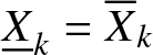 $\underline{X}_{k}=\overline{X}_{k}$. Furthermore, due to $0\leq\hat{\alpha}_{k}\leq\frac{1}{2}\leq\alpha_{k}\leq1$, it is obvious that $p''_{2}(q_{k}(t)) \lt 0$ for any admissible investment strategy. Hence, the first order optimality condition can be used to obtain the optimal investment strategy. Gathering the terms of $\omega_{k}(t)$ in the equations (A.6) and (A.10), let us define:
 \begin{equation}
\begin{aligned}
p_{3}(\omega_{k}(t))&=\eta\omega_{k}(t)E_{k}(t)+\alpha_{k}h^{p}\frac{1-2\exp(\beta_{k2}\underline{Y}_{k}-1)}{\beta_{k2}}+\hat{\alpha}_{k}h^{p}\frac{1-2\exp(-\beta_{k2}\overline{Y}_{k}-1)}{\beta_{k2}}.\\
\end{aligned}
\end{equation}
\begin{equation}
\begin{aligned}
p_{3}(\omega_{k}(t))&=\eta\omega_{k}(t)E_{k}(t)+\alpha_{k}h^{p}\frac{1-2\exp(\beta_{k2}\underline{Y}_{k}-1)}{\beta_{k2}}+\hat{\alpha}_{k}h^{p}\frac{1-2\exp(-\beta_{k2}\overline{Y}_{k}-1)}{\beta_{k2}}.\\
\end{aligned}
\end{equation}In addition, we can get
 \begin{equation}
\begin{aligned}
p'_{3}(\omega_{k}(t))&=\eta E_{k}(t)-\alpha_{k}h^{p}2\exp(\beta_{k2}Y_{k}-1)[\zeta E_{k}(t)+{\gamma_{k}}\underline{e}^{2}_{k}(t)\zeta^{2}(\omega_{k}(t)-n_{k}\omega_{l}(t))]\\
&+\hat{\alpha}_{k}h^{p}2\exp(-\beta_{k2}Y_{k}-1)[\zeta E_{k}(t)+{\gamma_{k}}\overline{e}^{2}_{k}(t)\zeta^{2}(\omega_{k}(t)-n_{k}\omega_{l}(t))]\\
\end{aligned}
\end{equation}
\begin{equation}
\begin{aligned}
p'_{3}(\omega_{k}(t))&=\eta E_{k}(t)-\alpha_{k}h^{p}2\exp(\beta_{k2}Y_{k}-1)[\zeta E_{k}(t)+{\gamma_{k}}\underline{e}^{2}_{k}(t)\zeta^{2}(\omega_{k}(t)-n_{k}\omega_{l}(t))]\\
&+\hat{\alpha}_{k}h^{p}2\exp(-\beta_{k2}Y_{k}-1)[\zeta E_{k}(t)+{\gamma_{k}}\overline{e}^{2}_{k}(t)\zeta^{2}(\omega_{k}(t)-n_{k}\omega_{l}(t))]\\
\end{aligned}
\end{equation}and
 \begin{equation}
\begin{aligned}
p''_{3}(\omega_{k}(t))&=-\alpha_{k}\beta_{k2}h^{p}2\exp(\beta_{k2}Y_{k}-1)[\zeta E_{k}(t)+{\gamma_{k}}\underline{e}^{2}_{k}(t)\zeta^{2}(\omega_{k}(t)-n_{k}\omega_{l}(t))]^{2}\\
&-\hat{\alpha}_{k}\beta_{k2}h^{p}2\exp(-\beta_{k2}Y_{k}-1)[\zeta E_{k}(t)+{\gamma_{k}}\overline{e}^{2}_{k}(t)\zeta^{2}(\omega_{k}(t)-n_{k}\omega_{l}(t))]^{2}\\
&-\alpha_{k}h^{p}2\exp(\beta_{k2}Y_{k}-1){\gamma_{k}}\underline{e}^{2}_{k}(t)\zeta^{2}+\hat{\alpha}_{k}h^{p}2\exp(-\beta_{k2}Y_{k}-1){\gamma_{k}}\overline{e}^{2}_{k}(t)\zeta^{2}
\end{aligned}
\end{equation}
\begin{equation}
\begin{aligned}
p''_{3}(\omega_{k}(t))&=-\alpha_{k}\beta_{k2}h^{p}2\exp(\beta_{k2}Y_{k}-1)[\zeta E_{k}(t)+{\gamma_{k}}\underline{e}^{2}_{k}(t)\zeta^{2}(\omega_{k}(t)-n_{k}\omega_{l}(t))]^{2}\\
&-\hat{\alpha}_{k}\beta_{k2}h^{p}2\exp(-\beta_{k2}Y_{k}-1)[\zeta E_{k}(t)+{\gamma_{k}}\overline{e}^{2}_{k}(t)\zeta^{2}(\omega_{k}(t)-n_{k}\omega_{l}(t))]^{2}\\
&-\alpha_{k}h^{p}2\exp(\beta_{k2}Y_{k}-1){\gamma_{k}}\underline{e}^{2}_{k}(t)\zeta^{2}+\hat{\alpha}_{k}h^{p}2\exp(-\beta_{k2}Y_{k}-1){\gamma_{k}}\overline{e}^{2}_{k}(t)\zeta^{2}
\end{aligned}
\end{equation} Similarly, it is not difficult to find that  $p''_{3}(\omega_{k}(t))\leq0$ for any admissible investment strategy. Hence, the first-order optimality condition can be used to obtain the optimal investment strategy. Let
 \begin{equation}
\begin{aligned}
&\overline{A_{k}}(t)=\gamma_k\beta^{2}(\alpha_{k}\underline{e}^{2}_{k}(t)+\hat{\alpha}_{k}(t)\overline{e}^{2}_{k}),~\overline{B_{k}}(t)=(\hat{\alpha}_{k}-\alpha_{k})\beta_{k1}\beta^{2}E^{2}_{k}.\\
\end{aligned}
\end{equation}
\begin{equation}
\begin{aligned}
&\overline{A_{k}}(t)=\gamma_k\beta^{2}(\alpha_{k}\underline{e}^{2}_{k}(t)+\hat{\alpha}_{k}(t)\overline{e}^{2}_{k}),~\overline{B_{k}}(t)=(\hat{\alpha}_{k}-\alpha_{k})\beta_{k1}\beta^{2}E^{2}_{k}.\\
\end{aligned}
\end{equation}Then, by solving the system of equations, we can obtain the optimal strategy as follows:
 \begin{equation}
\xi^{*}_{k}=\frac{\frac{\alpha E_{k}(t)}{\overline{A_{k}(t)}+\overline{B_{k}}(t)}+\frac{\alpha E_{l}(t)}{\overline{A_{l}(t)}+\overline{B_{l}(t)}}\frac{n_{k}\overline{A_{k}}(t)}{\overline{A_{k}}(t)+\overline{B_{k}}(t)}}{1-\frac{n_{k}\overline{A_{k}}(t)}{\overline{A_{k}}(t)+\overline{B_{k}(t)}}\frac{n_{l}\overline{A_{l}(t)}}{\overline{A_{l}}(t)+\overline{B_{l}}(t)}}\triangleq\overline{D^{\pi_{k}}_{kl}}(t).
\end{equation}
\begin{equation}
\xi^{*}_{k}=\frac{\frac{\alpha E_{k}(t)}{\overline{A_{k}(t)}+\overline{B_{k}}(t)}+\frac{\alpha E_{l}(t)}{\overline{A_{l}(t)}+\overline{B_{l}(t)}}\frac{n_{k}\overline{A_{k}}(t)}{\overline{A_{k}}(t)+\overline{B_{k}}(t)}}{1-\frac{n_{k}\overline{A_{k}}(t)}{\overline{A_{k}}(t)+\overline{B_{k}(t)}}\frac{n_{l}\overline{A_{l}(t)}}{\overline{A_{l}}(t)+\overline{B_{l}}(t)}}\triangleq\overline{D^{\pi_{k}}_{kl}}(t).
\end{equation}Substituting equations (4.10), (4.11), and (4.14) into (4.9), we can obtain
 \begin{align}&[\frac{\partial E_{k}(t)}{\partial t}+(A_{k}+\vartheta_{k})E_{k}(t)](\hat{x}_{k}+\vartheta_{k}y_{k}-n_{k}\vartheta_{l}y_{l})+\frac{\partial H(t)}{\partial t}+[d_{k}-(\lambda_k+\lambda)(1-q^{*}_{k})\mu_k\nonumber\\
&-\theta_k(1-q^{*}_{k})^{2}(\lambda_k+\lambda)\sigma^{2}_{k}-n_kd_{l}+n_k(\lambda_l+\lambda)(1-q^{*}_{l})\mu_l+n_k\theta_l(1-q^{*}_{l}(t))^{2}(\lambda_l+\lambda)\sigma^{2}_{l}\nonumber\\
&+\frac{\eta[\eta-2\zeta\alpha_{k}h^{p}\exp(\beta_{k2}Y^{*}_{k}-1)+2\zeta\hat{\alpha}_{k}h^{p}\exp(-\beta_{k2}Y^{*}_{k}-1)]E_{k}(t)}{2\hat{\alpha}_{k}h^{p}\exp(-\beta_{k2Y^{*}_{k}}-1)\gamma_{k}\underline{e}^{2}_{k}(t)-2\alpha_{k}h^{p}\exp(\beta_{k2Y^{*}_{k}}-1)\gamma_{k}\overline{e}^{2}_{k}(t)}]E_{k}(t)\nonumber\\
&+(\overline{D^{\pi_{k}}_{kl}}(t)-n_k\overline{D^{\pi_{l}}_{lk}}(t))\alpha E_{k}(t)-n_k(\hat{\alpha}_{k}-\alpha_{k})\overline{D^{\pi_{l}}_{lk}}(t)^{2}\beta^{2}E_{l}(t) E_{k}(t)\nonumber\\
&-\frac{\gamma}{2}(\overline{D^{\pi_{k}}_{kl}}(t)-n_k\overline{D^{\pi_{l}}_{lk}}(t))^{2}\beta^2(\alpha_{k}\underline{e^{2}_{k}}(t)+\hat{\alpha}_{k}\overline{e_{k}}^{2}(t))+\frac{(\hat{\alpha_{k}}-\alpha_{k})}{2}\beta_{k1}\beta^{2}\overline{D^{\pi_{k}}_{kl}(t)}E^{2}_{k}(t)\nonumber\\
&+\alpha_{k}h^{p}\frac{1-2\exp(\beta_{k2}Y^{*}_{k}-1)}{\beta_{k2}}+\hat{\alpha}_{k}h^{p}\frac{1-2\exp(-\beta_{k2}Y^{*}_{k}-1)}{\beta_{k2}}\nonumber\\
&+\alpha_{k}\int^{\infty}_{0}[1-\exp(\beta_{k3}\underline{X^{*}_{k}})]\upsilon_{k}(dy_{k})+\alpha_{k}\int^{\infty}_{0}[1-\exp(\beta_{k4}\underline{X^{*}_{k}})]\upsilon(dy_{k})\nonumber\\
&+\hat{\alpha}_{k}\int^{\infty}_{0}[1-\exp(-\beta_{k3}\overline{X^{*}_{k}})]\upsilon_{k}(dy_{k})+\hat{\alpha}_{k}\int^{\infty}_{0}[1-\exp(-\beta_{k4}\overline{X^{*}_{k}})]\upsilon(dy_{k})\}\}\nonumber\\
&+\alpha_{k}\int^{\infty}_{0}(n_{k}E_{k}(t)q^{*}_{l}y_{l}-\frac{\gamma_k}{2}n^{2}_{k}\underline{e^{2}_{k}}(q^{*}_{l})^{2}y^{2}_{l})\exp(\beta_{l3}\underline{X^{*}_{l}})\upsilon_{l}(dy_{l})\nonumber\\
&+\alpha_{k}\int^{\infty}_{0}(n_{k}E_{k}(t)q^{*}_{l}y_{l}-\frac{\gamma_k}{2}n^{2}_{k}\underline{e^{2}_{k}}(q^{*}_{l})^{2}y^{2}_{l})\exp(\beta_{l4}\underline{X^{*}_{l}})\upsilon(dy_{l})\nonumber\\
&+\hat{\alpha_{k}}\int^{\infty}_{0}(n_{k}E_{k}(t)q^{*}_{l}y_{l}-\frac{\gamma
_k}{2}n^{2}_{k}\overline{e_{k}}^{2}(q^{*}_{l})^{2}y^{2}_{l})\exp(-\beta_{l3}\overline{X^{*}_{l}})\upsilon_{l}(dy_{l})\nonumber\\
&+\hat{\alpha_{k}}\int^{\infty}_{0}(n_{k}E_{k}(t)q^{*}_{l}y_{l}-\frac{\gamma_k}{2}n^{2}_{k}\overline{e_{k}}^{2}(q^{*}_{l})^{2}y^{2}_{l})\exp(-\beta_{l4}\overline{X^{*}_{l}})\upsilon(dy_{l})=0.\end{align}
\begin{align}&[\frac{\partial E_{k}(t)}{\partial t}+(A_{k}+\vartheta_{k})E_{k}(t)](\hat{x}_{k}+\vartheta_{k}y_{k}-n_{k}\vartheta_{l}y_{l})+\frac{\partial H(t)}{\partial t}+[d_{k}-(\lambda_k+\lambda)(1-q^{*}_{k})\mu_k\nonumber\\
&-\theta_k(1-q^{*}_{k})^{2}(\lambda_k+\lambda)\sigma^{2}_{k}-n_kd_{l}+n_k(\lambda_l+\lambda)(1-q^{*}_{l})\mu_l+n_k\theta_l(1-q^{*}_{l}(t))^{2}(\lambda_l+\lambda)\sigma^{2}_{l}\nonumber\\
&+\frac{\eta[\eta-2\zeta\alpha_{k}h^{p}\exp(\beta_{k2}Y^{*}_{k}-1)+2\zeta\hat{\alpha}_{k}h^{p}\exp(-\beta_{k2}Y^{*}_{k}-1)]E_{k}(t)}{2\hat{\alpha}_{k}h^{p}\exp(-\beta_{k2Y^{*}_{k}}-1)\gamma_{k}\underline{e}^{2}_{k}(t)-2\alpha_{k}h^{p}\exp(\beta_{k2Y^{*}_{k}}-1)\gamma_{k}\overline{e}^{2}_{k}(t)}]E_{k}(t)\nonumber\\
&+(\overline{D^{\pi_{k}}_{kl}}(t)-n_k\overline{D^{\pi_{l}}_{lk}}(t))\alpha E_{k}(t)-n_k(\hat{\alpha}_{k}-\alpha_{k})\overline{D^{\pi_{l}}_{lk}}(t)^{2}\beta^{2}E_{l}(t) E_{k}(t)\nonumber\\
&-\frac{\gamma}{2}(\overline{D^{\pi_{k}}_{kl}}(t)-n_k\overline{D^{\pi_{l}}_{lk}}(t))^{2}\beta^2(\alpha_{k}\underline{e^{2}_{k}}(t)+\hat{\alpha}_{k}\overline{e_{k}}^{2}(t))+\frac{(\hat{\alpha_{k}}-\alpha_{k})}{2}\beta_{k1}\beta^{2}\overline{D^{\pi_{k}}_{kl}(t)}E^{2}_{k}(t)\nonumber\\
&+\alpha_{k}h^{p}\frac{1-2\exp(\beta_{k2}Y^{*}_{k}-1)}{\beta_{k2}}+\hat{\alpha}_{k}h^{p}\frac{1-2\exp(-\beta_{k2}Y^{*}_{k}-1)}{\beta_{k2}}\nonumber\\
&+\alpha_{k}\int^{\infty}_{0}[1-\exp(\beta_{k3}\underline{X^{*}_{k}})]\upsilon_{k}(dy_{k})+\alpha_{k}\int^{\infty}_{0}[1-\exp(\beta_{k4}\underline{X^{*}_{k}})]\upsilon(dy_{k})\nonumber\\
&+\hat{\alpha}_{k}\int^{\infty}_{0}[1-\exp(-\beta_{k3}\overline{X^{*}_{k}})]\upsilon_{k}(dy_{k})+\hat{\alpha}_{k}\int^{\infty}_{0}[1-\exp(-\beta_{k4}\overline{X^{*}_{k}})]\upsilon(dy_{k})\}\}\nonumber\\
&+\alpha_{k}\int^{\infty}_{0}(n_{k}E_{k}(t)q^{*}_{l}y_{l}-\frac{\gamma_k}{2}n^{2}_{k}\underline{e^{2}_{k}}(q^{*}_{l})^{2}y^{2}_{l})\exp(\beta_{l3}\underline{X^{*}_{l}})\upsilon_{l}(dy_{l})\nonumber\\
&+\alpha_{k}\int^{\infty}_{0}(n_{k}E_{k}(t)q^{*}_{l}y_{l}-\frac{\gamma_k}{2}n^{2}_{k}\underline{e^{2}_{k}}(q^{*}_{l})^{2}y^{2}_{l})\exp(\beta_{l4}\underline{X^{*}_{l}})\upsilon(dy_{l})\nonumber\\
&+\hat{\alpha_{k}}\int^{\infty}_{0}(n_{k}E_{k}(t)q^{*}_{l}y_{l}-\frac{\gamma
_k}{2}n^{2}_{k}\overline{e_{k}}^{2}(q^{*}_{l})^{2}y^{2}_{l})\exp(-\beta_{l3}\overline{X^{*}_{l}})\upsilon_{l}(dy_{l})\nonumber\\
&+\hat{\alpha_{k}}\int^{\infty}_{0}(n_{k}E_{k}(t)q^{*}_{l}y_{l}-\frac{\gamma_k}{2}n^{2}_{k}\overline{e_{k}}^{2}(q^{*}_{l})^{2}y^{2}_{l})\exp(-\beta_{l4}\overline{X^{*}_{l}})\upsilon(dy_{l})=0.\end{align}Combining equations (c) and (d) of (4.3) with (4.12), we can obtain the following system of equations by separating the variables:
 \begin{equation*}\qquad\qquad\qquad\quad
\begin{cases}
&\dfrac{\partial E_{k}(t)}{\partial t}+(A_{k}+\vartheta_{k})E_{k}(t),~~E_{k}(T)=1, \qquad\qquad\qquad\qquad\qquad\qquad\qquad\!\text{(A.23a)}\\
& \dfrac{\partial \underline{e_{k}}(t)}{\partial t}+(A_{k}+\vartheta_{k})\underline{e_{k}}(t),~~\underline{e_{k}}(T)=1, \qquad\qquad\qquad\qquad\qquad\qquad\qquad\,\text{(A.23b)}\\
& \dfrac{\partial \overline{e_{k}}(t)}{\partial t}+(A_{k}+\vartheta_{k})\overline{e_{k}}(t),~~\overline{e_{k}}(T)=1. \qquad\qquad\qquad\qquad\qquad\qquad\qquad\,\,\text{(A.23c)}
\end{cases}
\end{equation*}
\begin{equation*}\qquad\qquad\qquad\quad
\begin{cases}
&\dfrac{\partial E_{k}(t)}{\partial t}+(A_{k}+\vartheta_{k})E_{k}(t),~~E_{k}(T)=1, \qquad\qquad\qquad\qquad\qquad\qquad\qquad\!\text{(A.23a)}\\
& \dfrac{\partial \underline{e_{k}}(t)}{\partial t}+(A_{k}+\vartheta_{k})\underline{e_{k}}(t),~~\underline{e_{k}}(T)=1, \qquad\qquad\qquad\qquad\qquad\qquad\qquad\,\text{(A.23b)}\\
& \dfrac{\partial \overline{e_{k}}(t)}{\partial t}+(A_{k}+\vartheta_{k})\overline{e_{k}}(t),~~\overline{e_{k}}(T)=1. \qquad\qquad\qquad\qquad\qquad\qquad\qquad\,\,\text{(A.23c)}
\end{cases}
\end{equation*} \begin{align}&\frac{\partial \widetilde{H}_{k}(t)}{\partial t}+[d_{k}-(\lambda_k+\lambda)(1-q^{*}_{k})\mu_k-\theta_k(1-q^{*}_{k})^{2}(\lambda_k+\lambda)\sigma^{2}_{k}-n_kd_{l}+n_k(\lambda_l+\lambda)(1-q^{*}_{l})\mu_l\nonumber\\
&+n_k\theta_l(1-q^{*}_{l}(t))^{2}(\lambda_l+\lambda)\sigma^{2}_{l}+(\overline{D^{\pi_{k}}_{kl}(t)}-n_k\overline{D^{\pi_{l}}_{lk}(t)})\alpha E_{k}(t)-n_k(\hat{\alpha}_{k}-\alpha_{k})\overline{D^{\pi_{l}}_{lk}(t)}^{2}\beta^{2}E_{l}(t) E_{k}(t)\nonumber\\
&-\frac{\gamma}{2}(\overline{D^{\pi_{k}}_{kl}(t)}-n_k\overline{D^{\pi_{l}}_{lk}(t)})^{2}\beta^2(\alpha_{k}\underline{e^{2}_{k}}(t)+\hat{\alpha}_{k}\overline{e^{2}_{k}}(t))+\frac{(\hat{\alpha_{k}}-\alpha_{k})}{2}\beta_{k1}\beta^{2}\overline{D^{\pi_{k}}_{kl}(t)}E^{2}_{k}(t)\nonumber\\
&+\frac{\eta[\eta-2\zeta\alpha_{k}h^{p}\exp(\beta_{k2}Y^{*}_{k}-1)+2\zeta\hat{\alpha}_{k}h^{p}\exp(-\beta_{k2}Y^{*}_{k}-1)]E_{k}(t)}{2\hat{\alpha}_{k}h^{p}\exp(-\beta_{k2Y^{*}_{k}}-1)\gamma_{k}\underline{e}^{2}_{k}(t)-2\alpha_{k}h^{p}\exp(\beta_{k2Y^{*}_{k}}-1)\gamma_{k}\overline{e}^{2}_{k}(t)}]E_{k}(t)\nonumber\\
&+\alpha_{k}\int^{\infty}_{0}[1-\exp(\beta_{k3}\underline{X^{*}_{k}})]\upsilon_{k}(dy_{k})+\alpha_{k}\int^{\infty}_{0}[1-\exp(\beta_{k4}\underline{X^{*}_{k}})]\upsilon(dy_{k})\nonumber\\
&+\alpha_{k}h^{p}\frac{1-2\exp(\beta_{k2}Y^{*}_{k}-1)}{\beta_{k2}}+\hat{\alpha}_{k}h^{p}\frac{1-2\exp(-\beta_{k2}Y^{*}_{k}-1)}{\beta_{k2}}\nonumber\\
&+\hat{\alpha}_{k}\int^{\infty}_{0}[1-\exp(-\beta_{k3}\overline{X^{*}_{k}})]\upsilon_{k}(dy_{k})+\hat{\alpha}_{k}\int^{\infty}_{0}[1-\exp(-\beta_{k4}\overline{X^{*}_{k}})]\upsilon(dy_{k})\}\}\nonumber\\
&+\alpha_{k}\int^{\infty}_{0}(n_{k}E_{k}(t)q^{*}_{l}y_{l}-\frac{\gamma}{2}n^{2}_{k}\underline{e^{2}_{k}}(q^{*}_{l})^{2}y^{2}_{l})\exp(\beta_{l3}\underline{X^{*}_{l}})\upsilon_{l}(dy_{l})\nonumber\\
&+\alpha_{k}\int^{\infty}_{0}(n_{k}E_{k}(t)q^{*}_{l}y_{l}-\frac{\gamma}{2}n^{2}_{k}\underline{e^{2}_{k}}(q^{*}_{l})^{2}y^{2}_{l})\exp(\beta_{l4}\underline{X^{*}_{l}})\upsilon(dy_{l})\nonumber\\
&+\hat{\alpha_{k}}\int^{\infty}_{0}(n_{k}E_{k}(t)q^{*}_{l}y_{l}-\frac{\gamma}{2}n^{2}_{k}\overline{e^{2}_{k}}(q^{*}_{l})^{2}y^{2}_{l})\exp(-\beta_{l3}\overline{X^{*}_{l}})\upsilon_{l}(dy_{l})\nonumber\\
&+\hat{\alpha_{k}}\int^{\infty}_{0}(n_{k}E_{k}(t)q^{*}_{l}y_{l}-\frac{\gamma}{2}n^{2}_{k}\overline{e^{2}_{k}}(q^{*}_{l})^{2}y^{2}_{l})\exp(-\beta_{l4}\overline{X^{*}_{l}})\upsilon(dy_{l})=0,~~~~~\widetilde{H}_{k}(T)=0\end{align}
\begin{align}&\frac{\partial \widetilde{H}_{k}(t)}{\partial t}+[d_{k}-(\lambda_k+\lambda)(1-q^{*}_{k})\mu_k-\theta_k(1-q^{*}_{k})^{2}(\lambda_k+\lambda)\sigma^{2}_{k}-n_kd_{l}+n_k(\lambda_l+\lambda)(1-q^{*}_{l})\mu_l\nonumber\\
&+n_k\theta_l(1-q^{*}_{l}(t))^{2}(\lambda_l+\lambda)\sigma^{2}_{l}+(\overline{D^{\pi_{k}}_{kl}(t)}-n_k\overline{D^{\pi_{l}}_{lk}(t)})\alpha E_{k}(t)-n_k(\hat{\alpha}_{k}-\alpha_{k})\overline{D^{\pi_{l}}_{lk}(t)}^{2}\beta^{2}E_{l}(t) E_{k}(t)\nonumber\\
&-\frac{\gamma}{2}(\overline{D^{\pi_{k}}_{kl}(t)}-n_k\overline{D^{\pi_{l}}_{lk}(t)})^{2}\beta^2(\alpha_{k}\underline{e^{2}_{k}}(t)+\hat{\alpha}_{k}\overline{e^{2}_{k}}(t))+\frac{(\hat{\alpha_{k}}-\alpha_{k})}{2}\beta_{k1}\beta^{2}\overline{D^{\pi_{k}}_{kl}(t)}E^{2}_{k}(t)\nonumber\\
&+\frac{\eta[\eta-2\zeta\alpha_{k}h^{p}\exp(\beta_{k2}Y^{*}_{k}-1)+2\zeta\hat{\alpha}_{k}h^{p}\exp(-\beta_{k2}Y^{*}_{k}-1)]E_{k}(t)}{2\hat{\alpha}_{k}h^{p}\exp(-\beta_{k2Y^{*}_{k}}-1)\gamma_{k}\underline{e}^{2}_{k}(t)-2\alpha_{k}h^{p}\exp(\beta_{k2Y^{*}_{k}}-1)\gamma_{k}\overline{e}^{2}_{k}(t)}]E_{k}(t)\nonumber\\
&+\alpha_{k}\int^{\infty}_{0}[1-\exp(\beta_{k3}\underline{X^{*}_{k}})]\upsilon_{k}(dy_{k})+\alpha_{k}\int^{\infty}_{0}[1-\exp(\beta_{k4}\underline{X^{*}_{k}})]\upsilon(dy_{k})\nonumber\\
&+\alpha_{k}h^{p}\frac{1-2\exp(\beta_{k2}Y^{*}_{k}-1)}{\beta_{k2}}+\hat{\alpha}_{k}h^{p}\frac{1-2\exp(-\beta_{k2}Y^{*}_{k}-1)}{\beta_{k2}}\nonumber\\
&+\hat{\alpha}_{k}\int^{\infty}_{0}[1-\exp(-\beta_{k3}\overline{X^{*}_{k}})]\upsilon_{k}(dy_{k})+\hat{\alpha}_{k}\int^{\infty}_{0}[1-\exp(-\beta_{k4}\overline{X^{*}_{k}})]\upsilon(dy_{k})\}\}\nonumber\\
&+\alpha_{k}\int^{\infty}_{0}(n_{k}E_{k}(t)q^{*}_{l}y_{l}-\frac{\gamma}{2}n^{2}_{k}\underline{e^{2}_{k}}(q^{*}_{l})^{2}y^{2}_{l})\exp(\beta_{l3}\underline{X^{*}_{l}})\upsilon_{l}(dy_{l})\nonumber\\
&+\alpha_{k}\int^{\infty}_{0}(n_{k}E_{k}(t)q^{*}_{l}y_{l}-\frac{\gamma}{2}n^{2}_{k}\underline{e^{2}_{k}}(q^{*}_{l})^{2}y^{2}_{l})\exp(\beta_{l4}\underline{X^{*}_{l}})\upsilon(dy_{l})\nonumber\\
&+\hat{\alpha_{k}}\int^{\infty}_{0}(n_{k}E_{k}(t)q^{*}_{l}y_{l}-\frac{\gamma}{2}n^{2}_{k}\overline{e^{2}_{k}}(q^{*}_{l})^{2}y^{2}_{l})\exp(-\beta_{l3}\overline{X^{*}_{l}})\upsilon_{l}(dy_{l})\nonumber\\
&+\hat{\alpha_{k}}\int^{\infty}_{0}(n_{k}E_{k}(t)q^{*}_{l}y_{l}-\frac{\gamma}{2}n^{2}_{k}\overline{e^{2}_{k}}(q^{*}_{l})^{2}y^{2}_{l})\exp(-\beta_{l4}\overline{X^{*}_{l}})\upsilon(dy_{l})=0,~~~~~\widetilde{H}_{k}(T)=0\end{align} \begin{equation}
\begin{aligned}
&\frac{\partial\underline{\widetilde{h}}_{k}(t)}{\partial t}+[d_{k}-(\lambda_k+\lambda)(1-q_{k})\mu_k-\theta_k(1-q_{k})^{2}(\lambda_k+\lambda)\sigma^{2}_{k}-n_kd_{l}+n_k(\lambda_l+\lambda)(1-q^{*}_{l})\mu_l\\
&+n_k\theta_l(1-q^{*}_{l}(t))^{2}(\lambda_l+\lambda)\sigma^{2}_{l}+[(\underline{D^{\pi_{k}}_{kl}(t)}-n_k\underline{D^{\pi_{l}}_{lk}(t)})\alpha+(n_k\beta_{l1}\underline{D^{\pi_{l}}_{lk}(t)}-\beta_{k1}\underline{D^{\pi_{k}}_{kl}(t)})]\beta^{2}E_{k}(t)\underline{e_{k}}(t)\\
&+\frac{\eta[\eta-2\zeta\alpha_{k}h^{p}\exp(\beta_{k2}Y^{*}_{k}-1)+2\zeta\hat{\alpha}_{k}h^{p}\exp(-\beta_{k2}Y^{*}_{k}-1)]E_{k}(t)}{2\hat{\alpha}_{k}h^{p}\exp(-\beta_{k2Y^{*}_{k}}-1)\gamma_{k}\underline{e}^{2}_{k}(t)-2\alpha_{k}h^{p}\exp(\beta_{k2Y^{*}_{k}}-1)\gamma_{k}\overline{e}^{2}_{k}(t)}]\underline{e_{k}(t)}\\
&-\int^{\infty}_{0}\underline{e_{k}(t)}q^{*}_{k}(t)y_{k}\exp(\beta_{k3}\underline{X^{*}_{k}})\upsilon_{k}(dy_{k})\\
&+\exp(\beta_{k2}Y^{*}_{k}-1)\frac{h^{p}[\eta-2\zeta\alpha_{k}h^{p}\exp(\beta_{k2}Y^{*}_{k}-1)+2\zeta\hat{\alpha}_{k}h^{p}\exp(-\beta_{k2}Y^{*}_{k}-1)]E_{k}(t)}{2\hat{\alpha}_{k}h^{p}\exp(-\beta_{k2Y^{*}_{k}}-1)\gamma_{k}\underline{e}^{2}_{k}(t)-2\alpha_{k}h^{p}\exp(\beta_{k2Y^{*}_{k}}-1)\gamma_{k}\overline{e}^{2}_{k}(t)}
\end{aligned}
\end{equation}
\begin{equation}
\begin{aligned}
&\frac{\partial\underline{\widetilde{h}}_{k}(t)}{\partial t}+[d_{k}-(\lambda_k+\lambda)(1-q_{k})\mu_k-\theta_k(1-q_{k})^{2}(\lambda_k+\lambda)\sigma^{2}_{k}-n_kd_{l}+n_k(\lambda_l+\lambda)(1-q^{*}_{l})\mu_l\\
&+n_k\theta_l(1-q^{*}_{l}(t))^{2}(\lambda_l+\lambda)\sigma^{2}_{l}+[(\underline{D^{\pi_{k}}_{kl}(t)}-n_k\underline{D^{\pi_{l}}_{lk}(t)})\alpha+(n_k\beta_{l1}\underline{D^{\pi_{l}}_{lk}(t)}-\beta_{k1}\underline{D^{\pi_{k}}_{kl}(t)})]\beta^{2}E_{k}(t)\underline{e_{k}}(t)\\
&+\frac{\eta[\eta-2\zeta\alpha_{k}h^{p}\exp(\beta_{k2}Y^{*}_{k}-1)+2\zeta\hat{\alpha}_{k}h^{p}\exp(-\beta_{k2}Y^{*}_{k}-1)]E_{k}(t)}{2\hat{\alpha}_{k}h^{p}\exp(-\beta_{k2Y^{*}_{k}}-1)\gamma_{k}\underline{e}^{2}_{k}(t)-2\alpha_{k}h^{p}\exp(\beta_{k2Y^{*}_{k}}-1)\gamma_{k}\overline{e}^{2}_{k}(t)}]\underline{e_{k}(t)}\\
&-\int^{\infty}_{0}\underline{e_{k}(t)}q^{*}_{k}(t)y_{k}\exp(\beta_{k3}\underline{X^{*}_{k}})\upsilon_{k}(dy_{k})\\
&+\exp(\beta_{k2}Y^{*}_{k}-1)\frac{h^{p}[\eta-2\zeta\alpha_{k}h^{p}\exp(\beta_{k2}Y^{*}_{k}-1)+2\zeta\hat{\alpha}_{k}h^{p}\exp(-\beta_{k2}Y^{*}_{k}-1)]E_{k}(t)}{2\hat{\alpha}_{k}h^{p}\exp(-\beta_{k2Y^{*}_{k}}-1)\gamma_{k}\underline{e}^{2}_{k}(t)-2\alpha_{k}h^{p}\exp(\beta_{k2Y^{*}_{k}}-1)\gamma_{k}\overline{e}^{2}_{k}(t)}
\end{aligned}
\end{equation} \begin{equation*}
\begin{aligned}
&-\int^{\infty}_{0}\underline{e_{k}(t)}q^{*}_{k}(t)y_{k}\exp(\beta_{k4}\underline{X^{*}_{k}})\upsilon_{k}(dy_{k})-\int^{\infty}_{0}\underline{e_{k}(t)}n_{k}q^{*}_{l}(t)y_{l}\exp(\beta_{l3}\underline{X^{*}_{l}})\upsilon_{k}(dy_{l})\\
&-\int^{\infty}_{0}\underline{e_{k}(t)}n_{k}q^{*}_{l}(t)y_{l}\exp(\beta_{l4}\underline{X^{*}_{l}})\upsilon_{k}(dy_{l})=0,~~~~\underline{\widetilde{h}}_{k}(T)=0\\
\end{aligned}
\end{equation*}
\begin{equation*}
\begin{aligned}
&-\int^{\infty}_{0}\underline{e_{k}(t)}q^{*}_{k}(t)y_{k}\exp(\beta_{k4}\underline{X^{*}_{k}})\upsilon_{k}(dy_{k})-\int^{\infty}_{0}\underline{e_{k}(t)}n_{k}q^{*}_{l}(t)y_{l}\exp(\beta_{l3}\underline{X^{*}_{l}})\upsilon_{k}(dy_{l})\\
&-\int^{\infty}_{0}\underline{e_{k}(t)}n_{k}q^{*}_{l}(t)y_{l}\exp(\beta_{l4}\underline{X^{*}_{l}})\upsilon_{k}(dy_{l})=0,~~~~\underline{\widetilde{h}}_{k}(T)=0\\
\end{aligned}
\end{equation*} \begin{equation}
\begin{aligned}
&\frac{\partial\overline{\widetilde{h}}_{k}(t)}{\partial t}+[d_{k}-(\lambda_k+\lambda)(1-q_{k})\mu_k-\theta_k(1-q_{k})^{2}(\lambda_k+\lambda)\sigma^{2}_{k}-n_kd_{l}+n_k(\lambda_l+\lambda)(1-q^{*}_{l})\mu_l\\
&+n_k\theta_l(1-q^{*}_{l}(t))^{2}(\lambda_l+\lambda)\sigma^{2}_{l}+[(\overline{D^{\pi_{k}}_{kl}(t)}-n_k\overline{D^{\pi_{l}}_{lk}(t)})\alpha+(\beta_{k1}\overline{D^{\pi_{k}}_{kl}(t)}-n_k\beta_{l1}\overline{D^{\pi_{l}}_{lk}(t)})]\beta^{2}E_{k}(t)\overline{e_{k}}(t)\\
&+\frac{\eta[\eta-2\zeta\alpha_{k}h^{p}\exp(\beta_{k2}Y^{*}_{k}-1)+2\zeta\hat{\alpha}_{k}h^{p}\exp(-\beta_{k2}Y^{*}_{k}-1)]E_{k}(t)}{2\hat{\alpha}_{k}h^{p}\exp(-\beta_{k2Y^{*}_{k}}-1)\gamma_{k}\underline{e}^{2}_{k}(t)-2\alpha_{k}h^{p}\exp(\beta_{k2Y^{*}_{k}}-1)\gamma_{k}\overline{e}^{2}_{k}(t)}]\overline{e_{k}(t)}\\
&-\int^{\infty}_{0}\overline{e_{k}(t)}q^{*}_{k}(t)y_{k}\exp(-\beta_{k3}\overline{X^{*}_{k}})\upsilon_{k}(dy_{k})\\
&+\exp(-\beta_{k2}Y^{*}_{k}-1)\frac{h^{p}[\eta-2\zeta\alpha_{k}h^{p}\exp(\beta_{k2}Y^{*}_{k}-1)+2\zeta\hat{\alpha}_{k}h^{p}\exp(-\beta_{k2}Y^{*}_{k}-1)]E_{k}(t)}{2\hat{\alpha}_{k}h^{p}\exp(-\beta_{k2Y^{*}_{k}}-1)\gamma_{k}\underline{e}^{2}_{k}(t)-2\alpha_{k}h^{p}\exp(\beta_{k2Y^{*}_{k}}-1)\gamma_{k}\overline{e}^{2}_{k}(t)}\\
&-\int^{\infty}_{0}\overline{e_{k}(t)}q^{*}_{k}(t)y_{k}\exp(-\beta_{k4}\overline{X^{*}_{k}})\upsilon_{k}(dy_{k})-\int^{\infty}_{0}\overline{e_{k}(t)}n_{k}q^{*}_{l}(t)y_{l}\exp(-\beta_{l3}\overline{X^{*}_{l}})\upsilon_{k}(dy_{l})\\
&-\int^{\infty}_{0}\overline{e_{k}(t)}n_{k}q^{*}_{l}(t)y_{l}\exp(-\beta_{l4}\overline{X^{*}_{l}})\upsilon_{k}(dy_{l})=0,~~~~\overline{\widetilde{h}}_{k}(T)=0\\
\end{aligned}
\end{equation}
\begin{equation}
\begin{aligned}
&\frac{\partial\overline{\widetilde{h}}_{k}(t)}{\partial t}+[d_{k}-(\lambda_k+\lambda)(1-q_{k})\mu_k-\theta_k(1-q_{k})^{2}(\lambda_k+\lambda)\sigma^{2}_{k}-n_kd_{l}+n_k(\lambda_l+\lambda)(1-q^{*}_{l})\mu_l\\
&+n_k\theta_l(1-q^{*}_{l}(t))^{2}(\lambda_l+\lambda)\sigma^{2}_{l}+[(\overline{D^{\pi_{k}}_{kl}(t)}-n_k\overline{D^{\pi_{l}}_{lk}(t)})\alpha+(\beta_{k1}\overline{D^{\pi_{k}}_{kl}(t)}-n_k\beta_{l1}\overline{D^{\pi_{l}}_{lk}(t)})]\beta^{2}E_{k}(t)\overline{e_{k}}(t)\\
&+\frac{\eta[\eta-2\zeta\alpha_{k}h^{p}\exp(\beta_{k2}Y^{*}_{k}-1)+2\zeta\hat{\alpha}_{k}h^{p}\exp(-\beta_{k2}Y^{*}_{k}-1)]E_{k}(t)}{2\hat{\alpha}_{k}h^{p}\exp(-\beta_{k2Y^{*}_{k}}-1)\gamma_{k}\underline{e}^{2}_{k}(t)-2\alpha_{k}h^{p}\exp(\beta_{k2Y^{*}_{k}}-1)\gamma_{k}\overline{e}^{2}_{k}(t)}]\overline{e_{k}(t)}\\
&-\int^{\infty}_{0}\overline{e_{k}(t)}q^{*}_{k}(t)y_{k}\exp(-\beta_{k3}\overline{X^{*}_{k}})\upsilon_{k}(dy_{k})\\
&+\exp(-\beta_{k2}Y^{*}_{k}-1)\frac{h^{p}[\eta-2\zeta\alpha_{k}h^{p}\exp(\beta_{k2}Y^{*}_{k}-1)+2\zeta\hat{\alpha}_{k}h^{p}\exp(-\beta_{k2}Y^{*}_{k}-1)]E_{k}(t)}{2\hat{\alpha}_{k}h^{p}\exp(-\beta_{k2Y^{*}_{k}}-1)\gamma_{k}\underline{e}^{2}_{k}(t)-2\alpha_{k}h^{p}\exp(\beta_{k2Y^{*}_{k}}-1)\gamma_{k}\overline{e}^{2}_{k}(t)}\\
&-\int^{\infty}_{0}\overline{e_{k}(t)}q^{*}_{k}(t)y_{k}\exp(-\beta_{k4}\overline{X^{*}_{k}})\upsilon_{k}(dy_{k})-\int^{\infty}_{0}\overline{e_{k}(t)}n_{k}q^{*}_{l}(t)y_{l}\exp(-\beta_{l3}\overline{X^{*}_{l}})\upsilon_{k}(dy_{l})\\
&-\int^{\infty}_{0}\overline{e_{k}(t)}n_{k}q^{*}_{l}(t)y_{l}\exp(-\beta_{l4}\overline{X^{*}_{l}})\upsilon_{k}(dy_{l})=0,~~~~\overline{\widetilde{h}}_{k}(T)=0\\
\end{aligned}
\end{equation}Appendix B
Proof. For any fixed  $t\in[0,T]$, by letting
 \begin{equation}
\begin{aligned}
f_{k}(q_{k},y_{k})&=[(\lambda_{k}+\lambda)(y_{k}+2\theta_{k}(1-q^{*}_{k})y_{k}^{2})]E_{k}(t)\\
&-(\hat{\alpha}_{k}\exp(-\beta_{k3}{X^{*}_{k}})+\alpha_{k}\exp(\beta_{k3}{X^{*}_{k}}))\lambda_k(E_{k}(t)y_{k}+\gamma_{k}{e}^{2}_{k}y^{2}_{k}q^{*}_{k})\\
&-(\hat{\alpha}_{k}\exp(-\beta_{k4}{X^{*}_{k}})+\alpha_{k}\exp(\beta_{k4}{X^{*}_{k}}))\lambda(E_{k}(t)y_{k}+\gamma_{k}{e}^{2}_{k}y^{2}_{k}q^{*}_{k}),
\end{aligned}
\end{equation}
\begin{equation}
\begin{aligned}
f_{k}(q_{k},y_{k})&=[(\lambda_{k}+\lambda)(y_{k}+2\theta_{k}(1-q^{*}_{k})y_{k}^{2})]E_{k}(t)\\
&-(\hat{\alpha}_{k}\exp(-\beta_{k3}{X^{*}_{k}})+\alpha_{k}\exp(\beta_{k3}{X^{*}_{k}}))\lambda_k(E_{k}(t)y_{k}+\gamma_{k}{e}^{2}_{k}y^{2}_{k}q^{*}_{k})\\
&-(\hat{\alpha}_{k}\exp(-\beta_{k4}{X^{*}_{k}})+\alpha_{k}\exp(\beta_{k4}{X^{*}_{k}}))\lambda(E_{k}(t)y_{k}+\gamma_{k}{e}^{2}_{k}y^{2}_{k}q^{*}_{k}),
\end{aligned}
\end{equation}we can rewrite (4.8) as
 \begin{equation}
\begin{aligned}
\int^{\infty}_{0}f_{k}(q_{k},y_{k})dF(y_{k})=0.
\end{aligned}
\end{equation}
\begin{equation}
\begin{aligned}
\int^{\infty}_{0}f_{k}(q_{k},y_{k})dF(y_{k})=0.
\end{aligned}
\end{equation} Because 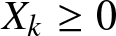 $X_{k}\geq0$ and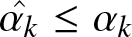 $\hat{\alpha_{k}}\leq\alpha_{k}$, we can obtain
 \begin{equation}
\begin{aligned}
\frac{\partial f_{k}(q_{k},y_{k})}{q_{k}}=&-(\lambda_{k}+\lambda)2\theta_{k}q^{*}_{k}y_{k}^{2}E_{k}(t)-(\hat{\alpha}_{k}\exp(-\beta_{k3}{X^{*}_{k}})+\alpha_{k}\exp(\beta_{k3}{X^{*}_{k}}))\lambda_k\gamma_{k}{e}^{2}_{k}y^{2}_{k}\\
&-(-\hat{\alpha}_{k}\beta_{k3}\exp(-\beta_{k3}{X^{*}_{k}})+\alpha_{k}\beta_{k3}\exp(\beta_{k3}{X^{*}_{k}}))\beta_{k3}\lambda_k(E_{k}(t)y_{k}+\gamma_{k}{e}^{2}_{k}y^{2}_{k}q^{*}_{k})^{2}\\
&-(-\hat{\alpha}_{k}\beta_{k4}\exp(-\beta_{k4}{X^{*}_{k}})+\alpha_{k}\beta_{k4}\exp(\beta_{k4}{X^{*}_{k}}))\lambda\beta_{k4}(E_{k}(t)y_{k}+\gamma_{k}{e}^{2}_{k}y^{2}_{k}q^{*}_{k})^{2}\\
&-(\hat{\alpha}_{k}\exp(-\beta_{k4}{X^{*}_{k}})+\alpha_{k}\exp(\beta_{k4}{X^{*}_{k}}))\lambda\gamma_{k}{e}^{2}_{k}y^{2}_{k}\leq0.
\end{aligned}
\end{equation}
\begin{equation}
\begin{aligned}
\frac{\partial f_{k}(q_{k},y_{k})}{q_{k}}=&-(\lambda_{k}+\lambda)2\theta_{k}q^{*}_{k}y_{k}^{2}E_{k}(t)-(\hat{\alpha}_{k}\exp(-\beta_{k3}{X^{*}_{k}})+\alpha_{k}\exp(\beta_{k3}{X^{*}_{k}}))\lambda_k\gamma_{k}{e}^{2}_{k}y^{2}_{k}\\
&-(-\hat{\alpha}_{k}\beta_{k3}\exp(-\beta_{k3}{X^{*}_{k}})+\alpha_{k}\beta_{k3}\exp(\beta_{k3}{X^{*}_{k}}))\beta_{k3}\lambda_k(E_{k}(t)y_{k}+\gamma_{k}{e}^{2}_{k}y^{2}_{k}q^{*}_{k})^{2}\\
&-(-\hat{\alpha}_{k}\beta_{k4}\exp(-\beta_{k4}{X^{*}_{k}})+\alpha_{k}\beta_{k4}\exp(\beta_{k4}{X^{*}_{k}}))\lambda\beta_{k4}(E_{k}(t)y_{k}+\gamma_{k}{e}^{2}_{k}y^{2}_{k}q^{*}_{k})^{2}\\
&-(\hat{\alpha}_{k}\exp(-\beta_{k4}{X^{*}_{k}})+\alpha_{k}\exp(\beta_{k4}{X^{*}_{k}}))\lambda\gamma_{k}{e}^{2}_{k}y^{2}_{k}\leq0.
\end{aligned}
\end{equation}Additionally,
 \begin{equation}
\begin{aligned}
f_{k}(0,y_{k})=(\lambda_{k}+\lambda)2\theta_{k}y_{k}^{2}E_{k}(t)\geq0.
\end{aligned}
\end{equation}
\begin{equation}
\begin{aligned}
f_{k}(0,y_{k})=(\lambda_{k}+\lambda)2\theta_{k}y_{k}^{2}E_{k}(t)\geq0.
\end{aligned}
\end{equation} Therefore, by the monotone convergence theorem and  $f_{k}(0,y_{k})=(\lambda_{k}+\lambda)2\theta_{k}y_{k}^{2}E_{k}(t)\geq0$, we can obtain
 \begin{equation}
\begin{aligned}
\lim_{q_{k}\downarrow0}\int^{\infty}_{0}f_{k}(q_{k},y_{k})dF(y_{k})=\int^{\infty}_{0}(\lambda_{k}+\lambda)2\theta_{k}y_{k}^{2}E_{k}(t)dF(y_{k})\geq0,
\end{aligned}
\end{equation}
\begin{equation}
\begin{aligned}
\lim_{q_{k}\downarrow0}\int^{\infty}_{0}f_{k}(q_{k},y_{k})dF(y_{k})=\int^{\infty}_{0}(\lambda_{k}+\lambda)2\theta_{k}y_{k}^{2}E_{k}(t)dF(y_{k})\geq0,
\end{aligned}
\end{equation}and
 \begin{equation}
\begin{aligned}
\lim_{q_{k}\uparrow\infty}\int^{\infty}_{0}f_{k}(q_{k},y_{k})dF(y_{k})=-\infty.
\end{aligned}
\end{equation}
\begin{equation}
\begin{aligned}
\lim_{q_{k}\uparrow\infty}\int^{\infty}_{0}f_{k}(q_{k},y_{k})dF(y_{k})=-\infty.
\end{aligned}
\end{equation} Hence, there exists a unique 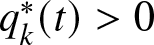 $q^{*}_{k}(t) \gt 0$ satisfying equation (4.9).
Appendix C
Proof. We show that  $q^{*}_{k}(t)$ is decreasing in $\alpha_{k}$. Hence, the proof process of the monotonicity in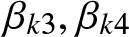 $\beta_{k3},\beta_{k4} $ and $\gamma_{k}$ can be demonstrated in the same way. We seek $\frac{\partial q^{*}_{k}(t)}{\partial\alpha_{k}}$ by differentiating equation (4.9) with respect to $\alpha_{k}$ as follows.
 \begin{equation}
\begin{aligned}
&-(\lambda_{k}+\lambda)2\theta_{k}\sigma_{k}^{2})E_{k}(t)\frac{\partial q^{*}_{k}}{\partial\alpha_{k}}\\
&-\int^{\infty}_{0}(-\exp(-\beta_{k3}{X^{*}_{k}})+\exp(\beta_{k3}{X^{*}_{k}}))(E_{k}(t)y_{k}+\gamma_{k}{e}^{2}_{k}y^{2}_{k}q^{*}_{k})\upsilon_{k}(dy_{k})\\
&-\int^{\infty}_{0}(\hat{\alpha}_{k}\exp(-\beta_{k3}{X^{*}_{k}})+\alpha_{k}\exp(\beta_{k3}{X^{*}_{k}}))(E_{k}(t)y_{k}+\gamma_{k}{e}^{2}_{k}y^{2}_{k}q^{*}_{k})^{2}\upsilon_{k}(dy_{k})\beta_{k3}(\alpha_{k}-\hat{\alpha}_k)\frac{\partial q^{*}_{k}}{\partial\alpha_{k}}\\
&-\int^{\infty}_{0}(\hat{\alpha}_{k}\exp(-\beta_{k3}{X^{*}_{k}})+\alpha_{k}\exp(\beta_{k3}{X^{*}_{k}}))\gamma_{k}{e}^{2}_{k}y^{2}_{k}\upsilon_{k}(dy_{k})\frac{\partial q^{*}_{k}}{\partial\alpha_{k}}\\
&-\int^{\infty}_{0}(-\exp(-\beta_{k4}{X^{*}_{k}})+\exp(\beta_{k4}{X^{*}_{k}}))(E_{k}(t)y_{k}+\gamma_{k}{e}^{2}_{k}y^{2}_{k}q^{*}_{k})\upsilon_{k}(dy_{k})\\
&-\int^{\infty}_{0}(\hat{\alpha}_{k}\exp(-\beta_{k4}{X^{*}_{k}})+\alpha_{k}\exp(\beta_{k4}{X^{*}_{k}}))(E_{k}(t)y_{k}+\gamma_{k}{e}^{2}_{k}y^{2}_{k}q^{*}_{k})^{2}\upsilon_{k}(dy_{k})\beta_{k4}(\alpha_{k}-\hat{\alpha}_k)\frac{\partial q^{*}_{k}}{\partial\alpha_{k}}\\
&-\int^{\infty}_{0}(\hat{\alpha}_{k}\exp(-\beta_{k4}{X^{*}_{k}})+\alpha_{k}\exp(\beta_{k4}{X^{*}_{k}}))\gamma_{k}{e}^{2}_{k}y^{2}_{k}\upsilon_{k}(dy_{k})\frac{\partial q^{*}_{k}}{\partial\alpha_{k}}=0.
\end{aligned}
\end{equation}
\begin{equation}
\begin{aligned}
&-(\lambda_{k}+\lambda)2\theta_{k}\sigma_{k}^{2})E_{k}(t)\frac{\partial q^{*}_{k}}{\partial\alpha_{k}}\\
&-\int^{\infty}_{0}(-\exp(-\beta_{k3}{X^{*}_{k}})+\exp(\beta_{k3}{X^{*}_{k}}))(E_{k}(t)y_{k}+\gamma_{k}{e}^{2}_{k}y^{2}_{k}q^{*}_{k})\upsilon_{k}(dy_{k})\\
&-\int^{\infty}_{0}(\hat{\alpha}_{k}\exp(-\beta_{k3}{X^{*}_{k}})+\alpha_{k}\exp(\beta_{k3}{X^{*}_{k}}))(E_{k}(t)y_{k}+\gamma_{k}{e}^{2}_{k}y^{2}_{k}q^{*}_{k})^{2}\upsilon_{k}(dy_{k})\beta_{k3}(\alpha_{k}-\hat{\alpha}_k)\frac{\partial q^{*}_{k}}{\partial\alpha_{k}}\\
&-\int^{\infty}_{0}(\hat{\alpha}_{k}\exp(-\beta_{k3}{X^{*}_{k}})+\alpha_{k}\exp(\beta_{k3}{X^{*}_{k}}))\gamma_{k}{e}^{2}_{k}y^{2}_{k}\upsilon_{k}(dy_{k})\frac{\partial q^{*}_{k}}{\partial\alpha_{k}}\\
&-\int^{\infty}_{0}(-\exp(-\beta_{k4}{X^{*}_{k}})+\exp(\beta_{k4}{X^{*}_{k}}))(E_{k}(t)y_{k}+\gamma_{k}{e}^{2}_{k}y^{2}_{k}q^{*}_{k})\upsilon_{k}(dy_{k})\\
&-\int^{\infty}_{0}(\hat{\alpha}_{k}\exp(-\beta_{k4}{X^{*}_{k}})+\alpha_{k}\exp(\beta_{k4}{X^{*}_{k}}))(E_{k}(t)y_{k}+\gamma_{k}{e}^{2}_{k}y^{2}_{k}q^{*}_{k})^{2}\upsilon_{k}(dy_{k})\beta_{k4}(\alpha_{k}-\hat{\alpha}_k)\frac{\partial q^{*}_{k}}{\partial\alpha_{k}}\\
&-\int^{\infty}_{0}(\hat{\alpha}_{k}\exp(-\beta_{k4}{X^{*}_{k}})+\alpha_{k}\exp(\beta_{k4}{X^{*}_{k}}))\gamma_{k}{e}^{2}_{k}y^{2}_{k}\upsilon_{k}(dy_{k})\frac{\partial q^{*}_{k}}{\partial\alpha_{k}}=0.
\end{aligned}
\end{equation} Hence, we define  $\phi(t)$ and $\varphi(t)$, respectively.
 \begin{equation}
\begin{aligned}
\phi(t)=&(\lambda_{k}+\lambda)2\theta_{k}\sigma_{k}^{2})E_{k}(t)+\int^{\infty}_{0}(\hat{\alpha}_{k}\exp(-\beta_{k3}{X^{*}_{k}})+\alpha_{k}\exp(\beta_{k3}{X^{*}_{k}}))\gamma_{k}{e}^{2}_{k}y^{2}_{k}\upsilon_{k}(dy_{k})\\
&+\int^{\infty}_{0}(\hat{\alpha}_{k}\exp(-\beta_{k3}{X^{*}_{k}})+\alpha_{k}\exp(\beta_{k3}{X^{*}_{k}}))(E_{k}(t)y_{k}+\gamma_{k}{e}^{2}_{k}y^{2}_{k}q^{*}_{k})^{2}\upsilon_{k}(dy_{k})\beta_{k3}(\alpha_{k}-\hat{\alpha}_k)\\
&+\int^{\infty}_{0}(\hat{\alpha}_{k}\exp(-\beta_{k4}{X^{*}_{k}})+\alpha_{k}\exp(\beta_{k4}{X^{*}_{k}}))(E_{k}(t)y_{k}+\gamma_{k}{e}^{2}_{k}y^{2}_{k}q^{*}_{k})^{2}\upsilon_{k}(dy_{k})\beta_{k4}(\alpha_{k}-\hat{\alpha}_k)\\
&+\int^{\infty}_{0}(\hat{\alpha}_{k}\exp(-\beta_{k4}{X^{*}_{k}})+\alpha_{k}\exp(\beta_{k4}{X^{*}_{k}}))\gamma_{k}{e}^{2}_{k}y^{2}_{k}\upsilon_{k}(dy_{k}),\\
\end{aligned}
\end{equation}
\begin{equation}
\begin{aligned}
\phi(t)=&(\lambda_{k}+\lambda)2\theta_{k}\sigma_{k}^{2})E_{k}(t)+\int^{\infty}_{0}(\hat{\alpha}_{k}\exp(-\beta_{k3}{X^{*}_{k}})+\alpha_{k}\exp(\beta_{k3}{X^{*}_{k}}))\gamma_{k}{e}^{2}_{k}y^{2}_{k}\upsilon_{k}(dy_{k})\\
&+\int^{\infty}_{0}(\hat{\alpha}_{k}\exp(-\beta_{k3}{X^{*}_{k}})+\alpha_{k}\exp(\beta_{k3}{X^{*}_{k}}))(E_{k}(t)y_{k}+\gamma_{k}{e}^{2}_{k}y^{2}_{k}q^{*}_{k})^{2}\upsilon_{k}(dy_{k})\beta_{k3}(\alpha_{k}-\hat{\alpha}_k)\\
&+\int^{\infty}_{0}(\hat{\alpha}_{k}\exp(-\beta_{k4}{X^{*}_{k}})+\alpha_{k}\exp(\beta_{k4}{X^{*}_{k}}))(E_{k}(t)y_{k}+\gamma_{k}{e}^{2}_{k}y^{2}_{k}q^{*}_{k})^{2}\upsilon_{k}(dy_{k})\beta_{k4}(\alpha_{k}-\hat{\alpha}_k)\\
&+\int^{\infty}_{0}(\hat{\alpha}_{k}\exp(-\beta_{k4}{X^{*}_{k}})+\alpha_{k}\exp(\beta_{k4}{X^{*}_{k}}))\gamma_{k}{e}^{2}_{k}y^{2}_{k}\upsilon_{k}(dy_{k}),\\
\end{aligned}
\end{equation}and
 \begin{equation}
\begin{aligned}
\varphi(t)=&\int^{\infty}_{0}(-\exp(-\beta_{k3}{X^{*}_{k}})+\exp(\beta_{k3}{X^{*}_{k}}))(E_{k}(t)y_{k}+\gamma_{k}{e}^{2}_{k}y^{2}_{k}q^{*}_{k})\upsilon_{k}(dy_{k})\\
&\int^{\infty}_{0}(-\exp(-\beta_{k4}{X^{*}_{k}})+\exp(\beta_{k4}{X^{*}_{k}}))(E_{k}(t)y_{k}+\gamma_{k}{e}^{2}_{k}y^{2}_{k}q^{*}_{k})\upsilon_{k}(dy_{k}).\\
\end{aligned}
\end{equation}
\begin{equation}
\begin{aligned}
\varphi(t)=&\int^{\infty}_{0}(-\exp(-\beta_{k3}{X^{*}_{k}})+\exp(\beta_{k3}{X^{*}_{k}}))(E_{k}(t)y_{k}+\gamma_{k}{e}^{2}_{k}y^{2}_{k}q^{*}_{k})\upsilon_{k}(dy_{k})\\
&\int^{\infty}_{0}(-\exp(-\beta_{k4}{X^{*}_{k}})+\exp(\beta_{k4}{X^{*}_{k}}))(E_{k}(t)y_{k}+\gamma_{k}{e}^{2}_{k}y^{2}_{k}q^{*}_{k})\upsilon_{k}(dy_{k}).\\
\end{aligned}
\end{equation}Therefore, we can have
 \begin{equation}
\begin{aligned}
&\phi(t)\frac{\partial q^{*}_{k}(t)}{\alpha_{k}}+\varphi(t)=0.
\end{aligned}
\end{equation}
\begin{equation}
\begin{aligned}
&\phi(t)\frac{\partial q^{*}_{k}(t)}{\alpha_{k}}+\varphi(t)=0.
\end{aligned}
\end{equation} Owing to 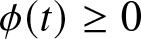 $\phi(t)\geq0$ and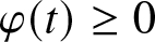 $\varphi(t)\geq0$, we have $\frac{\partial q^{*}_{k}(t)}{\alpha_{k}}\leq0$, i.e., $q^{*}_{k}(t)$ is decreasing in $\alpha_{k}$.


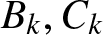


 Open access

