





1. Introduction
Broken rotational symmetry and orientationally ordered nematic phases are characteristic of fluids composed of anisotropic constituents, e.g. molecular liquid crystals (De Gennes & Prost Reference De Gennes and Prost1993), colloidal suspensions (Lewis et al. Reference Lewis, Garlea, Alvarado, Dammone, Howell, Majumdar, Mulder, Lettinga, Koenderink and Aarts2014; Nagel Reference Nagel2017) and biological matter (Maroudas-Sacks et al. Reference Maroudas-Sacks, Garion, Shani-Zerbib, Livshits, Braun and Keren2021; Doostmohammadi & Ladoux Reference Doostmohammadi and Ladoux2022). The continuum theory of nematic liquid crystals provides a fundamental framework for describing the dynamics of such complex fluids (Beris & Edwards Reference Beris and Edwards1994; Lettinga et al. Reference Lettinga, Dogic, Wang and Vermant2005; Saw et al. Reference Saw, Doostmohammadi, Nier, Kocgozlu, Thampi, Toyama, Marcq, Lim, Yeomans and Ladoux2017; Hadjifrangiskou, Thampi & Yeomans Reference Hadjifrangiskou, Thampi and Yeomans2025). The microstructure, namely the orientational order of anisotropic constituents, can be expressed using a symmetric, traceless tensor, called the nematic order parameter $\boldsymbol{Q}$
. In two dimensions (Giomi Reference Giomi2015; Shankar et al. Reference Shankar, Souslov, Bowick, Marchetti and Vitelli2022; Híjar & Majumdar Reference Híjar and Majumdar2024),
$\boldsymbol{Q}$
. In two dimensions (Giomi Reference Giomi2015; Shankar et al. Reference Shankar, Souslov, Bowick, Marchetti and Vitelli2022; Híjar & Majumdar Reference Híjar and Majumdar2024),
 \begin{align} \boldsymbol{Q}= \begin{pmatrix} Q_{xx} & Q_{xy}\\[3pt] Q_{xy} & -Q_{xx} \end{pmatrix} \equiv 2S\left (\boldsymbol{n}\boldsymbol{n}-\frac {1}{2}\boldsymbol{I}\right )\!, \end{align}
where the scalar $S$
gives the magnitude of nematic ordering, and the vector
$S$
gives the magnitude of nematic ordering, and the vector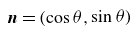 $\boldsymbol{n}=(\cos \theta , \sin \theta )$
describes the nematic director, the average orientation of the constituents. Thus
$\boldsymbol{n}=(\cos \theta , \sin \theta )$
describes the nematic director, the average orientation of the constituents. Thus $S$
and
$S$
and $\theta$
capture the two degrees of freedom in the nematic order tensor
$\theta$
capture the two degrees of freedom in the nematic order tensor $\boldsymbol{Q}$
. For isotropic fluids,
$\boldsymbol{Q}$
. For isotropic fluids, $S = 0$
, while for fully ordered nematic fluids,
$S = 0$
, while for fully ordered nematic fluids, $S = 1$
. In thermotropic and lyotropic molecular liquid crystals, temperature and concentration respectively dictate the strength of ordering
$S = 1$
. In thermotropic and lyotropic molecular liquid crystals, temperature and concentration respectively dictate the strength of ordering $S$
. In soft and biological matter, the additional dominant factors that determine
$S$
. In soft and biological matter, the additional dominant factors that determine $S$
may be the geometry of the constituents, and the non-equilibrium forcing and activity (Olmsted & Goldbart Reference Olmsted and Goldbart1992; Frenkel Reference Frenkel2015; Santhosh et al. Reference Santhosh, Nejad, Doostmohammadi, Yeomans and Thampi2020).
$S$
may be the geometry of the constituents, and the non-equilibrium forcing and activity (Olmsted & Goldbart Reference Olmsted and Goldbart1992; Frenkel Reference Frenkel2015; Santhosh et al. Reference Santhosh, Nejad, Doostmohammadi, Yeomans and Thampi2020).
When driven out of equilibrium either by an external forcing (Dubois-Violette, De Gennes & Parodi Reference Dubois-Violette, De Gennes and Parodi1971; Manneville Reference Manneville1981; Weiss & Ahlers Reference Weiss and Ahlers2013; Mur et al. Reference Mur, Kos, Ravnik and Muševič2022) or by an internal activity (Giomi Reference Giomi2015; Alert, Casademunt & Joanny Reference Alert, Casademunt and Joanny2022), nematic fluids display a wide range of steady and unsteady dynamic behaviours. Most theoretical studies that address the dynamics of nematic fluids employ the Ericksen–Leslie equations (Leslie Reference Leslie1968; Stewart Reference Stewart2004) which assume a uniform field for the magnitude of the order parameter $S$
, and only consider variations in the director field. This simplifies the analysis, and their widespread use may be due to the ease of visualisation of the director field in both experiments and computer simulations. Exceptions are studies that address the occurrence and dynamics of topological defects. Topological defects represent singularities in the
$S$
, and only consider variations in the director field. This simplifies the analysis, and their widespread use may be due to the ease of visualisation of the director field in both experiments and computer simulations. Exceptions are studies that address the occurrence and dynamics of topological defects. Topological defects represent singularities in the $\boldsymbol{Q}$
field; the core of the defect has
$\boldsymbol{Q}$
field; the core of the defect has $S = 0$
and an undefined director orientation. Then a description based on the Beris–Edwards model (Beris & Edwards Reference Beris and Edwards1994), which incorporates variations in nematic order
$S = 0$
and an undefined director orientation. Then a description based on the Beris–Edwards model (Beris & Edwards Reference Beris and Edwards1994), which incorporates variations in nematic order $S$
, is more natural. However, even in the latter theory, in practice, the role of order parameter variations is often neglected except in the vicinity of the topological defects.
$S$
, is more natural. However, even in the latter theory, in practice, the role of order parameter variations is often neglected except in the vicinity of the topological defects.
Of particular interest is the case of nematic liquid crystals subjected to pressure-driven flows in confined geometries. Early theoretical work was primarily based on Ericksen–Leslie theory (Leslie Reference Leslie1987). Further experimental and numerical studies (Jewell et al. Reference Jewell, Cornford, Yang, Cann and Sambles2009; Anderson et al. Reference Anderson, Mema, Kondic and Cummings2015; Batista et al. Reference Batista, Blow and Telo da Gama2015) have demonstrated that elastic and viscous stresses, together with anchoring conditions at the channel walls, can sustain multiple director configurations, giving rise to flow-driven transitions between distinct nematic states in Poiseuille-type flows. These competing states are often explained using free-energy considerations, with transitions occurring as the pressure gradient shifts the balance between anchoring-dominated and flow-aligned director fields. Subsequent extensions using the Beris–Edwards $\boldsymbol{Q}$
-tensor framework have allowed for systematic treatment of nematic order variations and topological defects, though many analyses continue to neglect order parameter variations away from defect cores (Sengupta et al. Reference Sengupta, Tkalec, Ravnik, Yeomans, Bahr and Herminghaus2013; Aplinc, Morris & Ravnik Reference Aplinc, Morris and Ravnik2016; Giomi et al. Reference Giomi, Kos, Ravnik and Sengupta2017). Recent theoretical studies have further characterised the solution landscapes and bifurcation structure of confined nematic flows, demonstrating how anchoring and confinement geometry mediate the coexistence of Bowser- and Dowser-like states (Crespo et al. Reference Crespo, Majumdar, Ramos del Olmo and Griffiths2017; Paul, Stellamanns & Sengupta Reference Paul, Stellamanns and Sengupta2021).
$\boldsymbol{Q}$
-tensor framework have allowed for systematic treatment of nematic order variations and topological defects, though many analyses continue to neglect order parameter variations away from defect cores (Sengupta et al. Reference Sengupta, Tkalec, Ravnik, Yeomans, Bahr and Herminghaus2013; Aplinc, Morris & Ravnik Reference Aplinc, Morris and Ravnik2016; Giomi et al. Reference Giomi, Kos, Ravnik and Sengupta2017). Recent theoretical studies have further characterised the solution landscapes and bifurcation structure of confined nematic flows, demonstrating how anchoring and confinement geometry mediate the coexistence of Bowser- and Dowser-like states (Crespo et al. Reference Crespo, Majumdar, Ramos del Olmo and Griffiths2017; Paul, Stellamanns & Sengupta Reference Paul, Stellamanns and Sengupta2021).
Microfluidic experiments using nematic fluids have revealed rich dynamical behaviour consistent with theoretical predictions. Flow-driven transitions between free-energy-driven and flow-aligned director structures have been observed in nematic channels with strong homeotropic anchoring (Jewell et al. Reference Jewell, Cornford, Yang, Cann and Sambles2009; Sengupta et al. Reference Sengupta, Tkalec, Ravnik, Yeomans, Bahr and Herminghaus2013). Recent experiments have demonstrated that careful control of channel geometry, boundary anchoring and flow rate can stabilise novel intermediate or chiral states (Čopar et al. Reference Čopar, Kos, Emeršič and Tkalec2020; İlhan et al. Reference İlhan, Carenza and Bukusoglu2025). Classically, Poiseuille-type flows in conjunction with an externally applied magnetic field have been used to manipulate the nematic order and thus determine the rheological properties of nematic liquid crystals (Kneppe, Schneider & Sharma Reference Kneppe, Schneider and Sharma1981; Olmsted & Goldbart Reference Olmsted and Goldbart1992). Together, these studies establish pressure-driven nematic flows as a canonical setting for probing the interplay of rheology, confinement, boundary conditions and hydrodynamic driving in nematic liquid crystals. However, most analyses have focused on reorienting director fields ( $\boldsymbol{n}$
) and their spatial variations, leaving open the role of the magnitude of nematic order (
$\boldsymbol{n}$
) and their spatial variations, leaving open the role of the magnitude of nematic order ( $S$
) and its variations in organising the equilibrium and dynamical states in nematic fluids.
$S$
) and its variations in organising the equilibrium and dynamical states in nematic fluids.
In this work, we use the Beris–Edwards $\boldsymbol{Q}$
-tensor formalism and demonstrate that even a slight, spatially uniform reduction in the magnitude of nematic order
$\boldsymbol{Q}$
-tensor formalism and demonstrate that even a slight, spatially uniform reduction in the magnitude of nematic order $S$
can fundamentally alter the equilibrium structure of confined nematic fluids. Specifically, we show that such ‘global melting’ – a spatially extended reduction of the scalar nematic order parameter away from its bulk equilibrium value – gives rise to new equilibrium configurations beyond those predicted by the theories that assume a constant nematic order. When the system is driven out of equilibrium through an imposed pressure gradient, these equilibria act as organising centres for complex dynamics, including bifurcations between competing configurations, oscillatory states and spatiotemporal chaos.
$S$
can fundamentally alter the equilibrium structure of confined nematic fluids. Specifically, we show that such ‘global melting’ – a spatially extended reduction of the scalar nematic order parameter away from its bulk equilibrium value – gives rise to new equilibrium configurations beyond those predicted by the theories that assume a constant nematic order. When the system is driven out of equilibrium through an imposed pressure gradient, these equilibria act as organising centres for complex dynamics, including bifurcations between competing configurations, oscillatory states and spatiotemporal chaos.
The paper is organised as follows. In § 2, we present the theoretical model. In § 3, we explore the equilibrium state of channel-confined nematic fluids (no external forcing). This is followed by analysis of one-dimensional, unidirectional steady and unsteady flows that nematic fluids develop under external forces in §§ 4 and 5, respectively. In § 6, we compare the one-dimensional results with numerical solutions of the full two-dimensional equations. We discuss the implications of the results and conclude in § 7.
2. Theoretical model
We consider an incompressible nematic liquid crystal confined in a two-dimensional planar channel with the coordinate $-\infty \lt x\lt \infty$
along the length of the channel, and the coordinate
$-\infty \lt x\lt \infty$
along the length of the channel, and the coordinate $-L/2\leqslant y \leqslant L/2$
along the width of the channel. This formulation assumes that anchoring and geometry suppress director and director distortions along the third dimension. In this regime, the dominant spatial variations occur across the channel width and along the flow direction, allowing the
$-L/2\leqslant y \leqslant L/2$
along the width of the channel. This formulation assumes that anchoring and geometry suppress director and director distortions along the third dimension. In this regime, the dominant spatial variations occur across the channel width and along the flow direction, allowing the $\boldsymbol{Q}$
-tensor to be treated as effectively two-dimensional. Similar reduced
$\boldsymbol{Q}$
-tensor to be treated as effectively two-dimensional. Similar reduced $\boldsymbol{Q}$
-tensor descriptions have frequently been employed in the analysis of nematic systems (see e.g. Giomi Reference Giomi2015; Golovaty, Montero & Sternberg Reference Golovaty, Montero and Sternberg2015; Shankar et al. Reference Shankar, Souslov, Bowick, Marchetti and Vitelli2022; Dalby et al. Reference Dalby, Han, Majumdar and Mrad2023; Híjar & Majumdar Reference Híjar and Majumdar2024).
$\boldsymbol{Q}$
-tensor descriptions have frequently been employed in the analysis of nematic systems (see e.g. Giomi Reference Giomi2015; Golovaty, Montero & Sternberg Reference Golovaty, Montero and Sternberg2015; Shankar et al. Reference Shankar, Souslov, Bowick, Marchetti and Vitelli2022; Dalby et al. Reference Dalby, Han, Majumdar and Mrad2023; Híjar & Majumdar Reference Híjar and Majumdar2024).
Several different continuum models exist for nematohydrodynamics, including director-based theories such as Ericksen–Leslie (Leslie Reference Leslie1968), tensor-based formulations such as Qian–Sheng (Qian & Sheng Reference Qian and Sheng1998), and kinetic-theory-based approaches (Doi & Edwards Reference Doi and Edwards1986); however, here we employ the widely-used Beris–Edwards model (Beris & Edwards Reference Beris and Edwards1994) because it captures spatial and temporal variations of the scalar order parameter, including defect-core structure and local suppression of nematic order, which are central to the multistability and flow-driven instabilities studied in this work. The Beris–Edwards nematohydrodynamic model (Beris & Edwards Reference Beris and Edwards1994) describes the dynamics of the system in terms of a velocity field $\boldsymbol{u}=(u_x,u_y)$
and the nematic order parameter field
$\boldsymbol{u}=(u_x,u_y)$
and the nematic order parameter field $\boldsymbol{Q}$
in (1.1).
$\boldsymbol{Q}$
in (1.1).
The governing Beris–Edwards equations read
 \begin{align} \partial _t Q_{ij} + u_k\, \partial _k Q_{ij} &= S_{ij} + \varGamma H_{ij}, \\[-12pt]\nonumber \end{align}
 \begin{align} \partial _i u_i &= 0, \\[-12pt]\nonumber \end{align}
 \begin{align} \rho \left ( \partial _t u_i + u_k\, \partial _k u_i \right ) &= \partial _{\!j} \sigma _{ij}, \end{align}
where $\rho$
is the mass density, and
$\rho$
is the mass density, and $\varGamma$
is the rotational viscosity. The strain rate and vorticity tensors are
$\varGamma$
is the rotational viscosity. The strain rate and vorticity tensors are $E_{ij} = (1/2)(\partial _i u_{\!j} + \partial _{\!j} u_i)$
and
$E_{ij} = (1/2)(\partial _i u_{\!j} + \partial _{\!j} u_i)$
and $\varOmega _{ij} = (1/2)(\partial _i u_{\!j} - \partial _{\!j} u_i)$
, respectively, the symmetric and antisymmetric parts of the velocity gradient tensor. Then the generalised co-rotational derivative (flow alignment term) is
$\varOmega _{ij} = (1/2)(\partial _i u_{\!j} - \partial _{\!j} u_i)$
, respectively, the symmetric and antisymmetric parts of the velocity gradient tensor. Then the generalised co-rotational derivative (flow alignment term) is
 \begin{align} S_{ij} &= (\lambda E_{ik} + \varOmega _{ik}) \left (Q_{kj} + \frac 12 \delta _{kj}\right ) + \left (Q_{ik} + \frac 12 \delta _{ik}\right ) (\lambda E_{kj} - \varOmega _{kj}) - 2\lambda \left (Q_{ij} + \frac 12 \delta _{ij}\right ) Q_{kl} \partial _k u_l, \end{align}
with the flow alignment parameter $\lambda$
. The molecular field
$\lambda$
. The molecular field $\boldsymbol{H}$
is defined as the variational derivative of Landau–de Gennes free energy
$\boldsymbol{H}$
is defined as the variational derivative of Landau–de Gennes free energy $\mathcal{F}_{\textit{nem}}=\int f\,{\rm d}^2\boldsymbol{x}$
as
$\mathcal{F}_{\textit{nem}}=\int f\,{\rm d}^2\boldsymbol{x}$
as
 \begin{equation} H_{ij} = - \frac {\partial f}{\partial Q_{ij}} + \partial _k \left ( \frac {\partial f}{\partial (\partial _k Q_{ij})} \right )\!. \end{equation}
We choose
 \begin{align} f = \frac {C}{2} \left ( S_{\textit{nem}}^2 - \frac 12 Q_{kl} Q_{lk} \right )^2 + \frac {K}{2}\, \partial _k Q_{ij}\, \partial _k Q_{ij}, \end{align}
yielding the explicit form
 \begin{equation} H_{ij} = C \left ( S_{\textit{nem}}^2 - \frac 12 Q_{kl}Q_{lk} \right ) Q_{ij} + K\, \partial _k \partial _k Q_{ij}. \end{equation}
Here, $S_{\textit{nem}}$
sets the magnitude of the nematic order parameter, which we set to
$S_{\textit{nem}}$
sets the magnitude of the nematic order parameter, which we set to $S_{\textit{nem}}=1$
, and
$S_{\textit{nem}}=1$
, and $C$
controls the stiffness of order parameter variations from
$C$
controls the stiffness of order parameter variations from $S_{\textit{nem}}$
. Equation (2.6) corresponds to a reduced Landau–de Gennes bulk potential below the isotropic–nematic transition, with the temperature dependence absorbed into material parameters (De Gennes & Prost Reference De Gennes and Prost1993) and
$S_{\textit{nem}}$
. Equation (2.6) corresponds to a reduced Landau–de Gennes bulk potential below the isotropic–nematic transition, with the temperature dependence absorbed into material parameters (De Gennes & Prost Reference De Gennes and Prost1993) and $S_{\textit{nem}}$
(Bhattacharyya & Yeomans Reference Bhattacharyya and Yeomans2023; Híjar & Majumdar Reference Híjar and Majumdar2024). The constant
$S_{\textit{nem}}$
(Bhattacharyya & Yeomans Reference Bhattacharyya and Yeomans2023; Híjar & Majumdar Reference Híjar and Majumdar2024). The constant $K$
is the elastic coefficient under the single elastic constant approximation, which is directly related to the Frank elasticity constant (Schiele & Trimper Reference Schiele and Trimper1983; Dammone et al. Reference Dammone, Zacharoudiou, Dullens, Yeomans, Lettinga and Aarts2012).
$K$
is the elastic coefficient under the single elastic constant approximation, which is directly related to the Frank elasticity constant (Schiele & Trimper Reference Schiele and Trimper1983; Dammone et al. Reference Dammone, Zacharoudiou, Dullens, Yeomans, Lettinga and Aarts2012).
The total stress field experienced by the nematic fluid combines the Newtonian viscous stress and a back flow stress,
 \begin{equation} \sigma _{ij} = - p \delta _{ij} + 2 \eta E_{ij} + (\sigma _B)_{ij}, \end{equation}
with
 \begin{align} (\sigma _B)_{ij} &= - \lambda H_{ik} \left (Q_{kj} + \frac 12 \delta _{kj}\right ) - \lambda \left (Q_{ik} + \frac 12 \delta _{ik}\right ) H_{kj} + 2\lambda \left (Q_{ij} + \frac 12 \delta _{ij}\right ) Q_{kl} H_{lk}\nonumber \\ &\quad {}- \frac {\partial f}{\partial (\partial _i Q_{kl})}\, \partial _{\!j} Q_{kl} + \big(Q_{ik}H_{kj} - H_{ik}Q_{kj}\big). \end{align}
In (2.8), $p$
denotes the isotropic pressure, and
$p$
denotes the isotropic pressure, and $\eta$
denotes the dynamic shear viscosity.
$\eta$
denotes the dynamic shear viscosity.
2.1. Dimensionless formulation
We non-dimensionalise the governing equations using the channel width $L$
as the length scale, and
$L$
as the length scale, and $U$
as a characteristic velocity scale. Time is scaled by
$U$
as a characteristic velocity scale. Time is scaled by $L/U$
, pressure by
$L/U$
, pressure by $\eta U/L$
, and the nematic order parameter by
$\eta U/L$
, and the nematic order parameter by $S_{\textit{nem}}$
.
$S_{\textit{nem}}$
.
With these definitions, the dimensionless Beris–Edwards equations may be written as (retaining the same symbols for the dimensionless variables)
 \begin{align} \partial _t Q_{ij} + u_k \partial _k Q_{ij} &= S_{ij} + \frac {1}{{\textit{Pe}}} H_{ij}, \\[-12pt]\nonumber \end{align}
 \begin{align} \partial _i u_i &= 0, \\[-12pt]\nonumber \end{align}
 \begin{align} {\textit{Re}} \left ( \partial _t u_i + u_k\, \partial _k u_i \right ) &= - \partial _i p + \partial _k \partial _k u_i + \frac {1}{{\textit{Er}}} \partial _{\!j} \hat {\sigma }_{B,ij} + f^{*}_{\textit{ext},i}. \end{align}
Here, $\boldsymbol{f}_{\textit{ext}}^{*}$
denotes the dimensionless external body force driving the flow, and
$\boldsymbol{f}_{\textit{ext}}^{*}$
denotes the dimensionless external body force driving the flow, and $\widehat {\boldsymbol{\sigma }}_{{B}}$
is the dimensionless nematic stress scaled by the elastic stress scale
$\widehat {\boldsymbol{\sigma }}_{{B}}$
is the dimensionless nematic stress scaled by the elastic stress scale $K/L^{2}$
. The flow-alignment term
$K/L^{2}$
. The flow-alignment term $\boldsymbol{S}$
retains the same functional form as in the dimensional equations. This process introduces the dimensionless parameters
$\boldsymbol{S}$
retains the same functional form as in the dimensional equations. This process introduces the dimensionless parameters
 \begin{equation} {\textit{Re}}=\frac {\rho \textit{UL}}{\eta }, \quad {\textit{Pe}}=\frac {U}{\varGamma \textit{CS}_{\textit{nem}}^{2} L}, \quad {\textit{Er}}=\frac {\eta \textit{UL}}{K}, \end{equation}
which compare inertia to viscous forces, advection to rotational diffusion, and viscous (or driving) stresses to elastic stresses, respectively. In addition, we define
 \begin{equation} \varepsilon =\frac {K}{\textit{CL}^{2}}, \end{equation}
which compares elastic to bulk nematic stiffness.
The dimensionless molecular field is
 \begin{equation} H_{ij} = \left ( 1 - \frac {1}{2} Q_{kl} Q_{lk} \right ) Q_{ij} + \varepsilon\, \partial _k \partial _k Q_{ij}, \end{equation}
and the dimensionless nematic stress $\widehat {\boldsymbol{\sigma }}_{{B}}$
retains the same structure as
$\widehat {\boldsymbol{\sigma }}_{{B}}$
retains the same structure as $\boldsymbol{\sigma }_{{B}}$
in the dimensional formulation, written in terms of the dimensionless fields
$\boldsymbol{\sigma }_{{B}}$
in the dimensional formulation, written in terms of the dimensionless fields $\boldsymbol{Q}$
and
$\boldsymbol{Q}$
and $\boldsymbol{H}$
. The dimensionless external body force
$\boldsymbol{H}$
. The dimensionless external body force $\boldsymbol{f}_{\textit{ext}}^{*}$
is related to the dimensional body force
$\boldsymbol{f}_{\textit{ext}}^{*}$
is related to the dimensional body force $\boldsymbol{f}_{\textit{ext}}=F\hat {\boldsymbol e}_{x}$
(force per unit volume) by the viscous stress scale, i.e.
$\boldsymbol{f}_{\textit{ext}}=F\hat {\boldsymbol e}_{x}$
(force per unit volume) by the viscous stress scale, i.e.
 \begin{align} \boldsymbol{f}_{\textit{ext}}^{*} = \frac {\boldsymbol{f}_{\textit{ext}}}{\eta U / L^2} = \frac {F L^{2}}{\eta U}\hat {\boldsymbol e}_{x}=f^*\hat {\boldsymbol e}_{x}. \end{align}
Unless stated otherwise, simulations are initialised with zero velocity and a uniform scalar order parameter $S=1$
. The initial director field
$S=1$
. The initial director field $\theta (y)$
is chosen either to be uniform or to have a linear variation across the channel width. Within the multistable regime, the final steady state depends on the initial director configuration, whereas outside this regime, the long-time dynamics is independent of initial conditions. In this work, ‘stability’ refers to dynamical stability with respect to perturbations within the reduced one- or two-dimensional Beris–Edwards dynamics considered here, as determined numerically from the long-time evolution of perturbed initial conditions.
$\theta (y)$
is chosen either to be uniform or to have a linear variation across the channel width. Within the multistable regime, the final steady state depends on the initial director configuration, whereas outside this regime, the long-time dynamics is independent of initial conditions. In this work, ‘stability’ refers to dynamical stability with respect to perturbations within the reduced one- or two-dimensional Beris–Edwards dynamics considered here, as determined numerically from the long-time evolution of perturbed initial conditions.
We impose strong homeotropic anchoring boundary conditions at the channel walls $\theta (-L/2)=\theta (L/2)=\pi /2$
, with
$\theta (-L/2)=\theta (L/2)=\pi /2$
, with $S(-L/2)=S(L/2)=1$
for the order parameter field, and no-slip, no-penetration boundary conditions
$S(-L/2)=S(L/2)=1$
for the order parameter field, and no-slip, no-penetration boundary conditions $\boldsymbol{u}(-L/2)=\boldsymbol{u}(L/2)=0$
for the velocity field. We drive the system out of equilibrium by applying a constant pressure gradient force
$\boldsymbol{u}(-L/2)=\boldsymbol{u}(L/2)=0$
for the velocity field. We drive the system out of equilibrium by applying a constant pressure gradient force $F$
along the positive
$F$
along the positive $x$
direction. When the unidirectional flow assumption is used in this paper, (2.1)–(2.3) reduce to a one-dimensional formalism as given in Appendix A. The resulting partial differential equations (A1) are solved in MATLAB by converting them to ordinary differential equations (ODEs) using the method of lines, with
$x$
direction. When the unidirectional flow assumption is used in this paper, (2.1)–(2.3) reduce to a one-dimensional formalism as given in Appendix A. The resulting partial differential equations (A1) are solved in MATLAB by converting them to ordinary differential equations (ODEs) using the method of lines, with $100$
units of space discretisation, and solving the resulting equations using the inbuilt solver ode45. When the fully two-dimensional system is considered, we use a hybrid lattice Boltzmann approach to obtain numerical solutions (Marenduzzo et al. Reference Marenduzzo, Orlandini, Cates and Yeomans2007; Thampi, Golestanian & Yeomans Reference Thampi, Golestanian and Yeomans2016). The incompressible Navier–Stokes equations are simulated in a
$100$
units of space discretisation, and solving the resulting equations using the inbuilt solver ode45. When the fully two-dimensional system is considered, we use a hybrid lattice Boltzmann approach to obtain numerical solutions (Marenduzzo et al. Reference Marenduzzo, Orlandini, Cates and Yeomans2007; Thampi, Golestanian & Yeomans Reference Thampi, Golestanian and Yeomans2016). The incompressible Navier–Stokes equations are simulated in a $100\times 20$
domain using a D2Q9 velocity set and a Guo forcing scheme (Guo, Zheng & Shi Reference Guo, Zheng and Shi2002; Krüger et al. Reference Krüger, Kusumaatmaja, Kuzmin, Shardt, Silva and Viggen2017), with periodic boundary conditions along the channel length. We use lattice Boltzmann units with spatial discretisation
$100\times 20$
domain using a D2Q9 velocity set and a Guo forcing scheme (Guo, Zheng & Shi Reference Guo, Zheng and Shi2002; Krüger et al. Reference Krüger, Kusumaatmaja, Kuzmin, Shardt, Silva and Viggen2017), with periodic boundary conditions along the channel length. We use lattice Boltzmann units with spatial discretisation $1$
unit and time step
$1$
unit and time step $1$
unit. The dynamics of
$1$
unit. The dynamics of $\boldsymbol{Q}$
is solved using an Euler–Maruyama finite difference method with time step 0.025. Other lattice Boltzmann fluid parameters were fixed as density
$\boldsymbol{Q}$
is solved using an Euler–Maruyama finite difference method with time step 0.025. Other lattice Boltzmann fluid parameters were fixed as density $\rho =20$
, and viscosity
$\rho =20$
, and viscosity $\eta =10/3$
. See the supplementary material available at https://doi.org/10.1017/jfm.2026.11800.
$\eta =10/3$
. See the supplementary material available at https://doi.org/10.1017/jfm.2026.11800.
Coexistence of multiple equilibrium states in channel-confined nematics with strong homeotropic anchoring. (a) Nematic order at the centre of the channel $S(0)$
as a function of the dimensionless parameter
$S(0)$
as a function of the dimensionless parameter $\epsilon = {K}/({\textit{CL}^2})$
. Simulations were performed by varying
$\epsilon = {K}/({\textit{CL}^2})$
. Simulations were performed by varying $K$
for fixed
$K$
for fixed $C=0.1$
and
$C=0.1$
and $L=20$
. The red line corresponds to a uniform
$L=20$
. The red line corresponds to a uniform $\boldsymbol{Q}$
/Bowser (B) state with constant nematic order
$\boldsymbol{Q}$
/Bowser (B) state with constant nematic order $S(y)=1$
. The blue line shows the variation of
$S(y)=1$
. The blue line shows the variation of $S(0)$
in a state with varying
$S(0)$
in a state with varying $\boldsymbol{Q}$
/Dowser (D). The varying
$\boldsymbol{Q}$
/Dowser (D). The varying $\boldsymbol{Q}$
state has a constant nematic order parameter
$\boldsymbol{Q}$
state has a constant nematic order parameter $S_0=1-2\pi ^2\epsilon$
(dashed blue line) in the bulk of the channel for small
$S_0=1-2\pi ^2\epsilon$
(dashed blue line) in the bulk of the channel for small $\epsilon$
, whereas strong spatial variations emerge in
$\epsilon$
, whereas strong spatial variations emerge in $S(y)$
for larger
$S(y)$
for larger $\epsilon$
. The yellow curve shows the numerically calculated boundary layer thickness
$\epsilon$
. The yellow curve shows the numerically calculated boundary layer thickness $\delta$
defined as the length from the boundary where nematic order reaches
$\delta$
defined as the length from the boundary where nematic order reaches $95\,\%\,S_0$
. The yellow dashed curve shows the fit
$95\,\%\,S_0$
. The yellow dashed curve shows the fit $2\delta /L=5\sqrt {\epsilon }$
. (b) Variations in the scalar nematic order
$2\delta /L=5\sqrt {\epsilon }$
. (b) Variations in the scalar nematic order $S$
and nematic orientation
$S$
and nematic orientation $\theta$
for the uniform
$\theta$
for the uniform $\boldsymbol{Q}$
/Bowser (B) state. (c,d) Corresponding plots for the varying
$\boldsymbol{Q}$
/Bowser (B) state. (c,d) Corresponding plots for the varying $\boldsymbol{Q}$
/Dowser (D) states for
$\boldsymbol{Q}$
/Dowser (D) states for $\epsilon =0.001$
and
$\epsilon =0.001$
and $\epsilon =0.03$
, respectively. Colour in greyscale indicates the scalar nematic order parameter
$\epsilon =0.03$
, respectively. Colour in greyscale indicates the scalar nematic order parameter $S$
. White lines show the director profile
$S$
. White lines show the director profile $\theta (y)$
across the channel. The dimensionless parameter
$\theta (y)$
across the channel. The dimensionless parameter $\epsilon$
compares the nematic correlation length to the channel width.
$\epsilon$
compares the nematic correlation length to the channel width.

3. Multiple equilibrium states in channel-confined nematics
We start by finding the states that minimise the free energy of the channel-confined nematic fluid in the absence of flow (absence of any external forces). Assuming translational invariance in the $x$
direction, and using
$x$
direction, and using $Q_{xx}=S \cos (2\theta )$
,
$Q_{xx}=S \cos (2\theta )$
, $Q_{xy}= S \sin (2\theta )$
, where
$Q_{xy}= S \sin (2\theta )$
, where $\theta \in (-\pi /2,\pi /2]$
in (2.1) and (2.7), results in the following ODEs for the nematic order field and the director field:
$\theta \in (-\pi /2,\pi /2]$
in (2.1) and (2.7), results in the following ODEs for the nematic order field and the director field:
 \begin{align} 0 &= \frac {{\rm d} ^2 S}{\text{d} y^2} - 4 S \left (\frac {\text{d} \theta }{\text{d} y} \right )^2 + \frac {C}{K} S (1 - S^2), \\[-12pt]\nonumber \end{align}
 \begin{align} 0 &= \frac {{\rm d}^2 \theta }{\text{d} y^2} + \frac {2 }{S} \frac {\text{d} \theta }{\text{d} y} \frac {\text{d} S}{\text{d} y}. \end{align}
Numerically solving (3.1)–(3.2), with strong homeotropic anchoring at the channel boundaries, we find multiple coexisting solutions.
As expected, the solution with uniform $\boldsymbol{Q}$
, i.e.
$\boldsymbol{Q}$
, i.e. $S(y)=1$
and
$S(y)=1$
and $\theta (y)=\pi /2$
(see figure 1
b), corresponds to the global minimum of the nematic free energy
$\theta (y)=\pi /2$
(see figure 1
b), corresponds to the global minimum of the nematic free energy $\mathcal{F}_{\textit{nem}}$
. However, there are also other solutions – where
$\mathcal{F}_{\textit{nem}}$
. However, there are also other solutions – where $\boldsymbol{Q}$
varies across the channel (see figure 1
c). These correspond to local minima of the free energy since spatial variations in
$\boldsymbol{Q}$
varies across the channel (see figure 1
c). These correspond to local minima of the free energy since spatial variations in $S$
and
$S$
and $\theta$
result in positive free-energy contributions. Although the spatially varying
$\theta$
result in positive free-energy contributions. Although the spatially varying $\boldsymbol{Q}$
states have a higher total free energy than the uniform state, their stability arises from a balance between elastic distortions of the director field and a reduction in the scalar order parameter, with the selected equilibrium determined by the basin of attraction set by the initial condition. They are topologically different to the uniform
$\boldsymbol{Q}$
states have a higher total free energy than the uniform state, their stability arises from a balance between elastic distortions of the director field and a reduction in the scalar order parameter, with the selected equilibrium determined by the basin of attraction set by the initial condition. They are topologically different to the uniform $\boldsymbol{Q}$
state in that they have
$\boldsymbol{Q}$
state in that they have $\theta =0$
at the centre of the channel, and an overall change in the nematic orientation from one wall to the other of
$\theta =0$
at the centre of the channel, and an overall change in the nematic orientation from one wall to the other of $n\pi$
. We will consider the single-twist states with
$n\pi$
. We will consider the single-twist states with $n=1$
in the remainder of this paper. We will refer to the uniform
$n=1$
in the remainder of this paper. We will refer to the uniform $\boldsymbol{Q}$
state as Bowser (B) and the
$\boldsymbol{Q}$
state as Bowser (B) and the $n=1$
varying
$n=1$
varying $\boldsymbol{Q}$
states as Dowser (D), since these steady states will give rise to the well-known Bowser and Dowser states (Čopar et al. Reference Čopar, Kos, Emeršič and Tkalec2020) in pressure-driven flows (see § 3).
$\boldsymbol{Q}$
states as Dowser (D), since these steady states will give rise to the well-known Bowser and Dowser states (Čopar et al. Reference Čopar, Kos, Emeršič and Tkalec2020) in pressure-driven flows (see § 3).
The Dowser states exist as degenerate pairs, distinguished by their chirality, D $^+$
and D
$^+$
and D $^-$
. For these states, the orientation (the director field) varies almost linearly across the channel
$^-$
. For these states, the orientation (the director field) varies almost linearly across the channel $\theta (y)\approx \pm \pi y/L$
. The spatial variation in the nematic order
$\theta (y)\approx \pm \pi y/L$
. The spatial variation in the nematic order $S$
can have two qualitatively different forms:
$S$
can have two qualitatively different forms:
-
(i) $S(y)$
constant but slightly less than unity in the bulk of the channel (figure 1
c);
$S(y)$
constant but slightly less than unity in the bulk of the channel (figure 1
c); -
(ii)
$S(y)$
has a smooth variation (a parabolic shape) across the channel (figure 1
d).


To quantify the crossover between these forms of $S(y)$
of the Dowser states, we define a dimensionless parameter
$S(y)$
of the Dowser states, we define a dimensionless parameter $\epsilon =K/({\textit{CL}}^2)$
that compares the nematic correlation length (
$\epsilon =K/({\textit{CL}}^2)$
that compares the nematic correlation length ( $\sqrt {K/C}$
) with the width of the channel (
$\sqrt {K/C}$
) with the width of the channel ( $L$
). Figure 1(a) shows the value of the scalar nematic order parameter at the centre of the channel
$L$
). Figure 1(a) shows the value of the scalar nematic order parameter at the centre of the channel $S(0)$
as a function of
$S(0)$
as a function of $\epsilon$
. Small
$\epsilon$
. Small $\epsilon$
corresponds to spatial variations in
$\epsilon$
corresponds to spatial variations in $S$
of the form (i), whereas larger values of
$S$
of the form (i), whereas larger values of $\epsilon$
correspond to
$\epsilon$
correspond to $S(y)$
of form (ii).
$S(y)$
of form (ii).
For the Dowser states at small $\epsilon$
, the value of the nematic order parameter can be approximated from (3.1) assuming a constant
$\epsilon$
, the value of the nematic order parameter can be approximated from (3.1) assuming a constant $S=S_0$
and a linearly varying director field. This results in a balance of contributions from free energies corresponding to nematic order and gradients in director giving
$S=S_0$
and a linearly varying director field. This results in a balance of contributions from free energies corresponding to nematic order and gradients in director giving
 \begin{align} 4 S \left (\frac {\partial \theta }{\partial y} \right )^2 \approx \frac {C}{K} S \big(1 - S^2\big). \end{align}
Using $\partial \theta /\partial y \approx \pi /L$
and
$\partial \theta /\partial y \approx \pi /L$
and $S\approx S_0$
, we get
$S\approx S_0$
, we get
 \begin{equation} S_0 \approx 1 - \frac {2 K \pi ^2}{\textit{CL}^2} = 1 - 2\pi ^2 \epsilon . \end{equation}
This equation (plotted as a dashed blue line in figure 1
a) shows that without any spatial variations in the nematic order $S$
in the channel bulk, a small, uniform decrease in the magnitude of the nematic order (
$S$
in the channel bulk, a small, uniform decrease in the magnitude of the nematic order ( $\approx 2\pi ^2 \epsilon$
) can support spatial (linear) variations in the orientation of the nematic field, and maintain the state of equilibrium.
$\approx 2\pi ^2 \epsilon$
) can support spatial (linear) variations in the orientation of the nematic field, and maintain the state of equilibrium.
We can further analyse the boundary layers that are formed for $S$
near the channel walls for small
$S$
near the channel walls for small $\epsilon$
. By non-dimensionalising the length scale with
$\epsilon$
. By non-dimensionalising the length scale with $L/2$
and performing a boundary layer analysis (see Appendix B), we obtain an asymptotic solution for the nematic order variations within the channel,
$L/2$
and performing a boundary layer analysis (see Appendix B), we obtain an asymptotic solution for the nematic order variations within the channel,
 \begin{align} S(y)=1-2\pi ^2\epsilon + 2\pi ^2\epsilon \left ({\rm e}^{-\frac{1-y}{\sqrt {2\epsilon }}} + {\rm e}^{-\frac{1+y}{\sqrt {2\epsilon }}} \right ) + O\big(\epsilon ^2\big). \end{align}
The boundary layer thickness is $\delta \propto \sqrt {\epsilon }$
. Figure 1(a) shows a comparison of this scaling (yellow dashed curve) with values calculated numerically (yellow solid curve).
$\delta \propto \sqrt {\epsilon }$
. Figure 1(a) shows a comparison of this scaling (yellow dashed curve) with values calculated numerically (yellow solid curve).
4. Unidirectional steady flows
Non-equilibrium steady flow states for pressure-driven nematics in a channel. (a) The nematic free energy $\mathcal{F}_{\textit{nem}}$
as a function of the applied pressure gradient force
$\mathcal{F}_{\textit{nem}}$
as a function of the applied pressure gradient force $F$
for B (red dots), D
$F$
for B (red dots), D $^-$
(blue dots) and D
$^-$
(blue dots) and D $^+$
(cyan dots) states. (b–d) The evolution of (top) nematic orientation
$^+$
(cyan dots) states. (b–d) The evolution of (top) nematic orientation $\theta$
, (middle) scalar nematic order
$\theta$
, (middle) scalar nematic order $S$
and (bottom) velocity
$S$
and (bottom) velocity $u_x$
for B, D
$u_x$
for B, D $^+$
and D
$^+$
and D $^-$
states, respectively. Bowser states originate from a uniform
$^-$
states, respectively. Bowser states originate from a uniform $\boldsymbol{Q}$
state at equilibrium (
$\boldsymbol{Q}$
state at equilibrium ( $F=0$
), whereas Dowser states originate from varying
$F=0$
), whereas Dowser states originate from varying $\boldsymbol{Q}$
states. The inset in (a) shows an example nematic configuration (
$\boldsymbol{Q}$
states. The inset in (a) shows an example nematic configuration ( $S(y)$
and
$S(y)$
and $\theta (y)$
) and velocity field (
$\theta (y)$
) and velocity field ( $u_x(y)$
) at
$u_x(y)$
) at $F=0.001$
for Bowser and Dowser states. Vertical dashed lines in (a) show the locations of instability of the D
$F=0.001$
for Bowser and Dowser states. Vertical dashed lines in (a) show the locations of instability of the D $^-$
and B states. Other parameters were fixed to
$^-$
and B states. Other parameters were fixed to $C=0.1$
,
$C=0.1$
, $K=0.01$
,
$K=0.01$
, $L=20$
,
$L=20$
, $\lambda =0$
. Choosing
$\lambda =0$
. Choosing $U$
to be the maximum velocity results in the following ranges for dimensionless parameters across the range of
$U$
to be the maximum velocity results in the following ranges for dimensionless parameters across the range of $F$
in the plot:
$F$
in the plot: $Re \in [0,3.5]$
,
$Re \in [0,3.5]$
, $Er \in [0,200]$
,
$Er \in [0,200]$
, $Pe \in [0,0.06]$
and
$Pe \in [0,0.06]$
and $\epsilon =0.001$
.
$\epsilon =0.001$
.

The Bowser (B) and Dowser (D $^\pm$
) states that correspond to free-energy minima of channel-confined nematics can be driven out of equilibrium by applying a pressure gradient
$^\pm$
) states that correspond to free-energy minima of channel-confined nematics can be driven out of equilibrium by applying a pressure gradient $F$
along the length of the channel. We investigate the variations of the steady states with
$F$
along the length of the channel. We investigate the variations of the steady states with $F$
by numerically solving the one-dimensional unidirectional flow equations (A1). At fixed forcing, Bowser and Dowser states coexist as dynamically stable steady solutions and are accessed from different initial conditions. The selected state is determined by the basin of attraction, reflecting multistability of the nematohydrodynamic equations. The forcing induces a Poiseuille-like unidirectional velocity field in the channel. As a result, the director orientation of each of the states begins to deviate from its equilibrium configuration, as shown in the inset of figure 2(a), and hence the nematic free energy increases. Importantly, we find that the steady states become unstable, one by one, with increasing
$F$
by numerically solving the one-dimensional unidirectional flow equations (A1). At fixed forcing, Bowser and Dowser states coexist as dynamically stable steady solutions and are accessed from different initial conditions. The selected state is determined by the basin of attraction, reflecting multistability of the nematohydrodynamic equations. The forcing induces a Poiseuille-like unidirectional velocity field in the channel. As a result, the director orientation of each of the states begins to deviate from its equilibrium configuration, as shown in the inset of figure 2(a), and hence the nematic free energy increases. Importantly, we find that the steady states become unstable, one by one, with increasing $F$
. The branches shown in figure 2 correspond to dynamically stable steady solutions; their termination marks the loss of stability of the corresponding branch. For the parameter combinations shown in figure 2, the D
$F$
. The branches shown in figure 2 correspond to dynamically stable steady solutions; their termination marks the loss of stability of the corresponding branch. For the parameter combinations shown in figure 2, the D $^-$
state becomes unstable first, followed by the instability of the B state, then eventually the instability of the D
$^-$
state becomes unstable first, followed by the instability of the B state, then eventually the instability of the D $^+$
state. In general, the order of instability of the states depends on the system parameters, and a different sequence of instabilities is found for different combinations of parameters (see Appendix C).
$^+$
state. In general, the order of instability of the states depends on the system parameters, and a different sequence of instabilities is found for different combinations of parameters (see Appendix C).
Contour plots showing variations in the nematic director, nematic order and unidirectional velocity field as functions of $F$
for the B, D
$F$
for the B, D $^+$
and D
$^+$
and D $^-$
states, respectively, are shown in figures 2(b–d). As
$^-$
states, respectively, are shown in figures 2(b–d). As $F$
is progressively increased, there is melting of the nematic order parameter
$F$
is progressively increased, there is melting of the nematic order parameter $S$
near the walls for the D
$S$
near the walls for the D $^-$
state, whereas for the B and D
$^-$
state, whereas for the B and D $^+$
states, we find a reduction in the nematic order both near the channel centre and near the channel walls. Furthermore, we see significant distortions of the nematic director field with increasing
$^+$
states, we find a reduction in the nematic order both near the channel centre and near the channel walls. Furthermore, we see significant distortions of the nematic director field with increasing $F$
in all three states, concentrated in the regions of lowest nematic ordering.
$F$
in all three states, concentrated in the regions of lowest nematic ordering.
The existence of Bowser and Dowser states has been reported in experiments with pressure-driven nematics where typically a transition from a Bowser to a Dowser state is observed with increasing flow rate in three-dimensional channel flows (Jewell et al. Reference Jewell, Cornford, Yang, Cann and Sambles2009; Sengupta et al. Reference Sengupta, Tkalec, Ravnik, Yeomans, Bahr and Herminghaus2013; Čopar et al. Reference Čopar, Kos, Emeršič and Tkalec2020; İlhan et al. Reference İlhan, Carenza and Bukusoglu2025). Attempts have been made in the literature to rationalise the Bowser–Dowser transitions using the Ericksen–Leslie equations that assume variations in only the nematic orientation (Jewell et al. Reference Jewell, Cornford, Yang, Cann and Sambles2009; Anderson et al. Reference Anderson, Mema, Kondic and Cummings2015; Batista et al. Reference Batista, Blow and Telo da Gama2015; Crespo et al. Reference Crespo, Majumdar, Ramos del Olmo and Griffiths2017; Paul et al. Reference Paul, Stellamanns and Sengupta2021). In the Ericksen–Leslie formalism, the two topologically distinct Bowser and Dowser flowing steady states cannot be simultaneously realised using different initial conditions, and one typically realises them via different anchoring boundary conditions at the channel walls. In this formalism, transition between the two states is usually interpreted using free-energy arguments where a Bowser–Dowser transition occurs because the Dowser state has a lower free energy at larger applied pressure gradient forces $F$
. The
$F$
. The $\boldsymbol{Q}$
-tensor formalism presented here, which takes into account both variations in nematic order and the nematic director, can support multistability, i.e. coexisting Bowser and Dowser states. This suggests that the transitions between Bowser and Dowser states that are observed in experiments might be due to a dynamical bifurcation (Strogatz Reference Strogatz2015), i.e. one of the states becoming unstable, and the system converging onto the remaining stable branch, as opposed to the system trying to minimise the nematic free energy.
$\boldsymbol{Q}$
-tensor formalism presented here, which takes into account both variations in nematic order and the nematic director, can support multistability, i.e. coexisting Bowser and Dowser states. This suggests that the transitions between Bowser and Dowser states that are observed in experiments might be due to a dynamical bifurcation (Strogatz Reference Strogatz2015), i.e. one of the states becoming unstable, and the system converging onto the remaining stable branch, as opposed to the system trying to minimise the nematic free energy.
However, we note that since the experiments are mostly performed with three-dimensional channels, the specific sequence and details of transitions that are observed might be dependent on the three-dimensional nature of the geometry. Nevertheless, the multistability of Bowser and Dowser states can be probed in experiments via hysteresis effects by e.g. starting in a Bowser state and slowly increasing the pressure gradient/flow rate up to the point of a Bowser–Dowser bifurcation, then slowly decreasing the pressure gradient/flow rate. If hysteresis is indeed observed in experiments, then it implies coexistence of Bowser–Dowser states in the underlying system.
Transition from steady to unsteady oscillatory states. (a–c) From left to right, kymographs of velocity field $u_x$
, nematic orientation
$u_x$
, nematic orientation $\theta$
, scalar nematic order
$\theta$
, scalar nematic order $S$
, and phase-space projection of the dynamics onto the two-dimensional space of global viscous dissipation
$S$
, and phase-space projection of the dynamics onto the two-dimensional space of global viscous dissipation $\mathcal{F}_{{vis}}$
and global free energy
$\mathcal{F}_{{vis}}$
and global free energy $\mathcal{F}_{\textit{nem}}$
(grey curves show transients, whereas black curves show the stable attractor). In (a),
$\mathcal{F}_{\textit{nem}}$
(grey curves show transients, whereas black curves show the stable attractor). In (a), $F=0.0032$
, where the system relaxes to the D
$F=0.0032$
, where the system relaxes to the D $^+$
steady state (cyan circle), whereas (b,c) correspond to
$^+$
steady state (cyan circle), whereas (b,c) correspond to $F=0.00324$
and
$F=0.00324$
and $F=0.0034$
, respectively, after the onset of oscillations. (d) The period
$F=0.0034$
, respectively, after the onset of oscillations. (d) The period $T$
of oscillations as a function of proximity to the transition; in the inset, a power-law scaling for the divergence of the form
$T$
of oscillations as a function of proximity to the transition; in the inset, a power-law scaling for the divergence of the form $T\propto |F-F_c|^{-1/2}$
is evident. Other parameters of the system are fixed at
$T\propto |F-F_c|^{-1/2}$
is evident. Other parameters of the system are fixed at $C=0.1 $
,
$C=0.1 $
, $K=0.01 $
,
$K=0.01 $
, $L=20$
and
$L=20$
and $\lambda =0$
.
$\lambda =0$
.

5. Unsteady unidirectional flows
Unsteady dynamics in pressure-driven nematic flows. (a) Bifurcation diagram showing peaks in the time series of the global free energy as functions of $F$
for the unidirectional, pressure-driven flow set-up. Initial flow velocity is zero,
$F$
for the unidirectional, pressure-driven flow set-up. Initial flow velocity is zero, $S=1$
, and different colours correspond to different initial orientation profiles, with red favouring B states, blue and cyan favouring D
$S=1$
, and different colours correspond to different initial orientation profiles, with red favouring B states, blue and cyan favouring D $^-$
and D
$^-$
and D $^+$
states, respectively, and grey corresponding to random initial orientations. (b–d) Kymographs of velocity, nematic orientation, scalar nematic order and phase-space trajectories (transients in grey, and stable attractors in black) for
$^+$
states, respectively, and grey corresponding to random initial orientations. (b–d) Kymographs of velocity, nematic orientation, scalar nematic order and phase-space trajectories (transients in grey, and stable attractors in black) for $F=0.008, 0.012, 0.018$
, respectively. Other parameters of the system are fixed at
$F=0.008, 0.012, 0.018$
, respectively. Other parameters of the system are fixed at $ C=0.1$
,
$ C=0.1$
, $K=0.01$
,
$K=0.01$
, $L=20$
and
$L=20$
and $\lambda =0$
. Choosing
$\lambda =0$
. Choosing $U$
to be the maximum velocity results in the following ranges for dimensionless parameters across the range of
$U$
to be the maximum velocity results in the following ranges for dimensionless parameters across the range of $F$
in the plot:
$F$
in the plot: $Re \in [0,35]$
,
$Re \in [0,35]$
, $Er \in [0,2000]$
,
$Er \in [0,2000]$
, $Pe \in [0,0.6]$
and
$Pe \in [0,0.6]$
and $\epsilon =0.001$
.
$\epsilon =0.001$
.

At large values of $F$
, beyond those shown in figure 2(a), all steady flows states become unstable, and the system enters an unsteady dynamical regime. At the onset of this regime, we find oscillatory states of the system. The transition from a steady state to an oscillatory state is illustrated in figures 3(a–c) for increasing values of
$F$
, beyond those shown in figure 2(a), all steady flows states become unstable, and the system enters an unsteady dynamical regime. At the onset of this regime, we find oscillatory states of the system. The transition from a steady state to an oscillatory state is illustrated in figures 3(a–c) for increasing values of $F$
. These plots show the kymograph of the unidirectional velocity field
$F$
. These plots show the kymograph of the unidirectional velocity field $u_x(y)$
, nematic orientation field
$u_x(y)$
, nematic orientation field $\theta (y)$
, and nematic order field
$\theta (y)$
, and nematic order field $S(y)$
, together with a phase-space projection in the space of the global nematic free energy
$S(y)$
, together with a phase-space projection in the space of the global nematic free energy $\mathcal{F}_{\textit{nem}}$
, and the global viscous dissipation associated with the fluid flow
$\mathcal{F}_{\textit{nem}}$
, and the global viscous dissipation associated with the fluid flow $\mathcal{F}_{{vis}}$
, defined as
$\mathcal{F}_{{vis}}$
, defined as
 \begin{align} \mathcal{F}_{{vis}}=\int _{-L/2}^{L/2} \frac {\eta }{2}\left (\frac {1}{2}\frac {\partial u_x}{\partial y}\right )^2\, {\rm d}y. \end{align}
Projecting the dynamics onto the space of total nematic free energy and total viscous dissipation provides a compact global view of the system’s energetic evolution, enabling clear identification of steady states, periodic orbits and chaotic regimes in an otherwise high-dimensional dynamical system.
The oscillating state corresponds to cyclical transitions between (unstable) Bowser-like and Dowser-like states, i.e. the time-dependent nematic field resembles either Bowser- or Dowser-type steady states instantaneously. Since these states are topologically distinct, i.e. they differ in the winding of the director across the channel width, the periodic transitions between them are mediated by topological transitions, i.e. a continuous line resembling a line of defects in the two-dimensional channel. This can be inferred from the kymograph of the nematic orientation and the nematic order shown in figures 3(b,c), where the nematic order parameter $S$
goes to zero. Note that
$S$
goes to zero. Note that $S$
goes to zero at the centre or near the walls of the channel. The oscillatory nature of the flow emerges from the coupling of the nematic field and the velocity field in the nematohydrodynamic model.
$S$
goes to zero at the centre or near the walls of the channel. The oscillatory nature of the flow emerges from the coupling of the nematic field and the velocity field in the nematohydrodynamic model.
We observe oscillating states with very large period $T$
at the onset of the transition, and the oscillation period decreases progressively with increasing
$T$
at the onset of the transition, and the oscillation period decreases progressively with increasing $F$
as shown in figure 3(d). Furthermore, we obtain a power-law scaling behaviour (see inset) for the divergence of the oscillation period as a function of the proximity to the transition of the form
$F$
as shown in figure 3(d). Furthermore, we obtain a power-law scaling behaviour (see inset) for the divergence of the oscillation period as a function of the proximity to the transition of the form $T\propto |F-F_c|^{-1/2}$
, where
$T\propto |F-F_c|^{-1/2}$
, where $F_c\approx 0.00321$
is the critical value of
$F_c\approx 0.00321$
is the critical value of $F$
where the bifurcation from steady flow to oscillatory flow occurs. A critical exponent
$F$
where the bifurcation from steady flow to oscillatory flow occurs. A critical exponent $-1/2$
is a characteristic of saddle-node type bifurcations (Strogatz Reference Strogatz2015), and suggests that the onset of oscillations takes place via an infinite-period bifurcation as opposed to a Hopf bifurcation that is ubiquitously associated with the onset of oscillations for many nonlinear dynamical systems. This is further evident from the phase-space trajectory in figure 3(a) just before the bifurcation, where the trajectory performs a large excursion, almost traversing the limit cycle, before converging onto the D
$-1/2$
is a characteristic of saddle-node type bifurcations (Strogatz Reference Strogatz2015), and suggests that the onset of oscillations takes place via an infinite-period bifurcation as opposed to a Hopf bifurcation that is ubiquitously associated with the onset of oscillations for many nonlinear dynamical systems. This is further evident from the phase-space trajectory in figure 3(a) just before the bifurcation, where the trajectory performs a large excursion, almost traversing the limit cycle, before converging onto the D $^+$
stable point (cyan circle). This suggests that the D
$^+$
stable point (cyan circle). This suggests that the D $^+$
fixed point loses stability in a saddle-node bifurcation, and the resulting emergence of oscillations is via a saddle-node, infinite-period (SNIPER) bifurcation.
$^+$
fixed point loses stability in a saddle-node bifurcation, and the resulting emergence of oscillations is via a saddle-node, infinite-period (SNIPER) bifurcation.
To characterise the full sequence of transitions with increasing $F$
, we plot a bifurcation diagram spanning both the steady and the unsteady regimes in figure 4(a). The quantities that we choose to plot in the bifurcation diagram are the peak values in the time series of global nematic free energy, i.e.
$F$
, we plot a bifurcation diagram spanning both the steady and the unsteady regimes in figure 4(a). The quantities that we choose to plot in the bifurcation diagram are the peak values in the time series of global nematic free energy, i.e. $\mathcal{F}_{\textit{nem}}(t_n)$
, where
$\mathcal{F}_{\textit{nem}}(t_n)$
, where $t_n$
are time stamps corresponding to local maxima in the free energy. In the steady regime, since
$t_n$
are time stamps corresponding to local maxima in the free energy. In the steady regime, since $\mathcal{F}_{\textit{nem}}$
is a constant, this would correspond to a single point on the bifurcation diagram. In the unsteady regime, a finite set of points correspond to periodic motion, whereas scattered points typically correspond to chaotic or quasi-periodic dynamics.
$\mathcal{F}_{\textit{nem}}$
is a constant, this would correspond to a single point on the bifurcation diagram. In the unsteady regime, a finite set of points correspond to periodic motion, whereas scattered points typically correspond to chaotic or quasi-periodic dynamics.
To detect and characterise the presence of multistability, i.e. the existence of different states at the same parameter values, the bifurcation diagram is created by solving the one-dimensional equations of motion (A1) with different initial profiles for the nematic orientation field $\theta (y,t=0)$
. We choose
$\theta (y,t=0)$
. We choose
 \begin{align} \theta _{B}(y,t=0)&=\frac {\pi }{2}+\frac {F}{12K(\eta \varGamma +1)} y \left (\left (\frac {L}{2}\right )^2-y^2\right )\!, \nonumber \\ \theta _{D+}(y,t=0)&=\frac {\pi }{L}y+\frac {F}{12K(\eta \varGamma +1)} y \left (\left (\frac {L}{2}\right )^2-y^2\right )\!, \nonumber \\ \theta _{D-}(y,t=0)&=-\frac {\pi }{L}y+\frac {F}{12K(\eta \varGamma +1)} y \left (\left (\frac {L}{2}\right )^2-y^2\right )\!, \nonumber \\ \theta _{R}(y,t=0)&=\left [\frac {-\pi }{2},\frac {\pi }{2}\right ]+\frac {F}{12K(\eta \varGamma +1)} y \left (\left (\frac {L}{2}\right )^2-y^2\right )\!. \end{align}
The first terms in these expressions correspond to the orientations of the B, D $^+$
and D
$^+$
and D $^-$
states at equilibrium, or R, a random initial orientation where
$^-$
states at equilibrium, or R, a random initial orientation where $\theta _R(y,0)$
is uniformly sampled in
$\theta _R(y,0)$
is uniformly sampled in $[{-\pi }/{2}, {\pi }/{2}]$
, respectively. The second terms account for the distortions in the nematic orientation due to an applied Poiseuille flow velocity profile for a constant scalar nematic order field. The initial nematic order field is set to
$[{-\pi }/{2}, {\pi }/{2}]$
, respectively. The second terms account for the distortions in the nematic orientation due to an applied Poiseuille flow velocity profile for a constant scalar nematic order field. The initial nematic order field is set to $S(y,t=0)=1$
, and the unidirectional velocity field is set to
$S(y,t=0)=1$
, and the unidirectional velocity field is set to $u_x(y,t=0)=0$
.
$u_x(y,t=0)=0$
.
The solutions are shown in figure 4(a) as red for states favouring Bowser configurations, $\theta _B(y,0)$
, cyan for Dowser D
$\theta _B(y,0)$
, cyan for Dowser D $^+$
,
$^+$
, $\theta _{D+}(y,0)$
, dark blue for Dowser D
$\theta _{D+}(y,0)$
, dark blue for Dowser D $^-$
,
$^-$
, $\theta _{D-}(y,0)$
, and grey for random initial orientations,
$\theta _{D-}(y,0)$
, and grey for random initial orientations, $\theta _{R}(y,0)$
. The steady regime of the bifurcation diagram is similar to figure 2(a) for initial conditions favouring Bowser and Dowser states, whereas random initial conditions take the system to higher-order Dowser states with
$\theta _{R}(y,0)$
. The steady regime of the bifurcation diagram is similar to figure 2(a) for initial conditions favouring Bowser and Dowser states, whereas random initial conditions take the system to higher-order Dowser states with $n\gt 1$
. (We note that in figure 2(a), we used numerical continuation to follow the steady branches when they are stable, whereas here we solve the partial differential equations with the initial conditions specified above.) Once all the steady states (grey region) become unstable, we first see oscillatory unsteady behaviour from
$n\gt 1$
. (We note that in figure 2(a), we used numerical continuation to follow the steady branches when they are stable, whereas here we solve the partial differential equations with the initial conditions specified above.) Once all the steady states (grey region) become unstable, we first see oscillatory unsteady behaviour from $F\approx 0.0034$
to
$F\approx 0.0034$
to $F\approx 0.007$
, with chaotic behaviour first emerging beyond
$F\approx 0.007$
, with chaotic behaviour first emerging beyond $F\approx 0.007$
, for initial conditions favouring Bowser and Dowser states. By contrast, for random initial conditions, the scattered dots indicate chaos for almost all values of
$F\approx 0.007$
, for initial conditions favouring Bowser and Dowser states. By contrast, for random initial conditions, the scattered dots indicate chaos for almost all values of $F$
in the unsteady regime. We also notice from the bifurcation diagram that if the initial conditions are not random, then the system does not permanently maintain chaos for large
$F$
in the unsteady regime. We also notice from the bifurcation diagram that if the initial conditions are not random, then the system does not permanently maintain chaos for large $F$
in the unsteady regime, and we find alternating regimes of periodic and chaotic behaviours with increasing
$F$
in the unsteady regime, and we find alternating regimes of periodic and chaotic behaviours with increasing $F$
– a feature that is common in bifurcation diagrams of low-dimensional chaotic systems (Strogatz Reference Strogatz2015).
$F$
– a feature that is common in bifurcation diagrams of low-dimensional chaotic systems (Strogatz Reference Strogatz2015).
Kymographs of the chaotic dynamics with increasing $F$
beyond
$F$
beyond $F\approx 0.007$
are displayed in figures 4(b–d). These show that although the dynamical behaviour is not entirely periodic, its chaotic nature is weak. There is periodicity on short time scales, with period decreasing with
$F\approx 0.007$
are displayed in figures 4(b–d). These show that although the dynamical behaviour is not entirely periodic, its chaotic nature is weak. There is periodicity on short time scales, with period decreasing with $F$
, and irregularities emerging at longer time scales spanning several periods. This is further evident from the phase-space trajectories, which show the system traversing a chaotic attractor with some structure, a signature of low-dimensional chaos (Strogatz Reference Strogatz2015). The almost periodic nature of the chaos is also evident from the bifurcation diagram, where in the chaotic regime, the points are not scattered uniformly but are concentrated near periodic branches. These results provide evidence that beyond the periodic regime, the system transitions to weak spatiotemporal chaos. The dynamics is governed by the interplay between free-energy relaxation via the molecular field, co-rotational coupling of the nematic tensor to the local velocity gradient, and the backflow stress entering the momentum equation. For small forcing, elastic and viscous effects dominate, leading to steady solutions. As the forcing increases, vorticity-driven reorientation of the nematic field and the resulting backflow feedback destabilise the steady branches, producing oscillatory dynamics and, at larger forcing, defect-mediated spatiotemporal chaos.
$F$
, and irregularities emerging at longer time scales spanning several periods. This is further evident from the phase-space trajectories, which show the system traversing a chaotic attractor with some structure, a signature of low-dimensional chaos (Strogatz Reference Strogatz2015). The almost periodic nature of the chaos is also evident from the bifurcation diagram, where in the chaotic regime, the points are not scattered uniformly but are concentrated near periodic branches. These results provide evidence that beyond the periodic regime, the system transitions to weak spatiotemporal chaos. The dynamics is governed by the interplay between free-energy relaxation via the molecular field, co-rotational coupling of the nematic tensor to the local velocity gradient, and the backflow stress entering the momentum equation. For small forcing, elastic and viscous effects dominate, leading to steady solutions. As the forcing increases, vorticity-driven reorientation of the nematic field and the resulting backflow feedback destabilise the steady branches, producing oscillatory dynamics and, at larger forcing, defect-mediated spatiotemporal chaos.
Thus a unidirectional, pressure-driven nematic exhibits a variety of dynamical regimes: steady flows, unsteady periodic flows and spatiotemporal chaos (see Appendix C for bifurcation diagrams for other parameter values).
Nematohydrodynamics in two-dimensional pressure-driven channel flows. (a) Bifurcation diagram analogous to figure 4(a) for the full two-dimensional equations of motion (2.1)–(2.3). In two-dimensional flows, multistability is observed between different unsteady dynamical states. (b,e) For example, at $F=0.0024$
, spatial uniform initial conditions along
$F=0.0024$
, spatial uniform initial conditions along $x$
corresponding to a Bowser or a Dowser configuration result in periodic states where the whole channel periodically transitions between a Bowser-like and a Dowser-like state. (c, f) Conversely, if the initial conditions are random, then defects are stabilised by advection along the channel. This results in weakly chaotic flow, as the defect dynamics is not entirely periodic. (d,g) At a higher value
$x$
corresponding to a Bowser or a Dowser configuration result in periodic states where the whole channel periodically transitions between a Bowser-like and a Dowser-like state. (c, f) Conversely, if the initial conditions are random, then defects are stabilised by advection along the channel. This results in weakly chaotic flow, as the defect dynamics is not entirely periodic. (d,g) At a higher value $F=0.006$
, the turbulent flow becomes more prominent through the continuous formation, annihilation and advection of defects. The kymographs in (e–g) are shown for a fixed
$F=0.006$
, the turbulent flow becomes more prominent through the continuous formation, annihilation and advection of defects. The kymographs in (e–g) are shown for a fixed $x=50$
. Other parameter values are the same as for figure 4. Choosing
$x=50$
. Other parameter values are the same as for figure 4. Choosing $U$
to be the maximum velocity results in the following ranges for dimensionless parameters across the range of
$U$
to be the maximum velocity results in the following ranges for dimensionless parameters across the range of $F$
in the plot:
$F$
in the plot: $Re \in [0,18]$
,
$Re \in [0,18]$
, $Er \in [0,1000]$
,
$Er \in [0,1000]$
, $Pe \in [0,0.3]$
and
$Pe \in [0,0.3]$
and $\epsilon =0.001$
.
$\epsilon =0.001$
.

6. Unsteady flows in a two-dimensional channel
We now solve the full two-dimensional nematohydrodynamic equations of motion (2.1)–(2.3) using a hybrid lattice Boltzmann algorithm (Marenduzzo et al. Reference Marenduzzo, Orlandini, Cates and Yeomans2007; Thampi et al. Reference Thampi, Golestanian and Yeomans2016).
Analogous to figure 4(a), we consider pressure-driven two-dimensional channel flows, and create a bifurcation diagram as a function of $F$
, as shown in figure 5(a). To most easily compare the flow dynamics between two dimensions and one dimension, we choose the bifurcation parameters as the peak values in the time series of the nematic free energy calculated at a fixed
$F$
, as shown in figure 5(a). To most easily compare the flow dynamics between two dimensions and one dimension, we choose the bifurcation parameters as the peak values in the time series of the nematic free energy calculated at a fixed $x$
location along the channel and integrated across the width
$x$
location along the channel and integrated across the width $y$
of the channel. The nematic free energy is computed by evaluating the Landau–de Gennes free-energy density at each lattice node using (2.6) (gradients are evaluated using a finite-difference formula), and summing this contribution over the domain. The initial conditions are chosen to be the same as those for the bifurcation diagram in figure 4(a), (5.2), i.e. the velocity field is initialised as
$y$
of the channel. The nematic free energy is computed by evaluating the Landau–de Gennes free-energy density at each lattice node using (2.6) (gradients are evaluated using a finite-difference formula), and summing this contribution over the domain. The initial conditions are chosen to be the same as those for the bifurcation diagram in figure 4(a), (5.2), i.e. the velocity field is initialised as $\boldsymbol{u}(x,y,0)=0$
throughout the domain, the scalar order parameter is initialised as
$\boldsymbol{u}(x,y,0)=0$
throughout the domain, the scalar order parameter is initialised as $S(x,y,0)=1$
, and the imposed pressure gradient
$S(x,y,0)=1$
, and the imposed pressure gradient $F$
is applied at
$F$
is applied at $t=0$
and held fixed during the time evolution. The initial director field only varies in the
$t=0$
and held fixed during the time evolution. The initial director field only varies in the $y$
direction for the Dowser and Bowser favouring configurations (5.2).
$y$
direction for the Dowser and Bowser favouring configurations (5.2).
For small values of $F$
, we find Bowser and Dowser steady flowing states (grey region), and they undergo the same sequence of instabilities as observed in the one-dimensional formalism. Further, we ubiquitously find multistability between steady and unsteady states, as well as between different types of unsteady states. In particular, for
$F$
, we find Bowser and Dowser steady flowing states (grey region), and they undergo the same sequence of instabilities as observed in the one-dimensional formalism. Further, we ubiquitously find multistability between steady and unsteady states, as well as between different types of unsteady states. In particular, for $F\sim 0.0015$
(light grey region in figure 5
a), the steady states coexist with a dynamic advecting defect state. Initial conditions that favour Bowser or Dowser states indeed lead to Bowser or Dowser steady states with variations in orientation only in the
$F\sim 0.0015$
(light grey region in figure 5
a), the steady states coexist with a dynamic advecting defect state. Initial conditions that favour Bowser or Dowser states indeed lead to Bowser or Dowser steady states with variations in orientation only in the $y$
direction as for the one-dimensional model. However, if the initial conditions are random, then there are many
$y$
direction as for the one-dimensional model. However, if the initial conditions are random, then there are many $+1/2$
and
$+1/2$
and $-1/2$
topological defects (Doostmohammadi et al. Reference Doostmohammadi, Ignés-Mullol, Yeomans and Sagués2018) present in the initial state. Not all of these are able to annihilate each other, and they are advected down the channel by the applied pressure gradient.
$-1/2$
topological defects (Doostmohammadi et al. Reference Doostmohammadi, Ignés-Mullol, Yeomans and Sagués2018) present in the initial state. Not all of these are able to annihilate each other, and they are advected down the channel by the applied pressure gradient.
With increasing $F$
, there is multistability in unsteady states as well. For example, for
$F$
, there is multistability in unsteady states as well. For example, for $F=0.0024$
, Bowser-like or Dowser-like initial conditions lead to the entire two-dimensional channel undergoing uniform periodic oscillations between a Bowser and a Dowser state (figure 5
b). The kymographs of the velocity field, nematic orientation, nematic order and phase-space trajectory, which are plotted for a fixed
$F=0.0024$
, Bowser-like or Dowser-like initial conditions lead to the entire two-dimensional channel undergoing uniform periodic oscillations between a Bowser and a Dowser state (figure 5
b). The kymographs of the velocity field, nematic orientation, nematic order and phase-space trajectory, which are plotted for a fixed $x$
in figure 5(e), are similar to those obtained in one dimension (compare figures 3
a–c). Instead, if the system is started with random initial conditions, then we obtain advecting defects, showing signs of weak chaos, as shown by the snapshot in figure 5(c). The corresponding kymographs are shown in figure 5( f).
$x$
in figure 5(e), are similar to those obtained in one dimension (compare figures 3
a–c). Instead, if the system is started with random initial conditions, then we obtain advecting defects, showing signs of weak chaos, as shown by the snapshot in figure 5(c). The corresponding kymographs are shown in figure 5( f).
Further increases in $F$
lead to more irregular motion of defects, i.e. spatiotemporal chaos or topological turbulence, where defects are created and annihilated as they advect down the channel as shown in figure 5(d), with the corresponding kymographs in figure 5(g). Note that
$F$
lead to more irregular motion of defects, i.e. spatiotemporal chaos or topological turbulence, where defects are created and annihilated as they advect down the channel as shown in figure 5(d), with the corresponding kymographs in figure 5(g). Note that $+1/2$
defects are typically found near the centre of the channel, whereas
$+1/2$
defects are typically found near the centre of the channel, whereas $-1/2$
defects are found near the channel walls. This is consistent with the turbulent state observed in the one-dimensional model, and also with variations in the nematic order observed in steady states for large
$-1/2$
defects are found near the channel walls. This is consistent with the turbulent state observed in the one-dimensional model, and also with variations in the nematic order observed in steady states for large $F$
(see figure 2
a); in both cases, the nematic order melts most strongly near the channel centre or walls.
$F$
(see figure 2
a); in both cases, the nematic order melts most strongly near the channel centre or walls.
The essence of spatiotemporal chaos in two-dimensional driven nematics that we report here lies in the irregular dynamics of topological defects as they are created, annihilated and advected down the channel due to an applied strong pressure-gradient $F$
. The creation and annihilation of the defects is a reflection of local topological transition between Bowser-like and Dowser-like states. To show this more clearly, we consider an advecting defect state at
$F$
. The creation and annihilation of the defects is a reflection of local topological transition between Bowser-like and Dowser-like states. To show this more clearly, we consider an advecting defect state at $F=0.0014$
obtained from random initial conditions. After initial transients, we obtain advecting pairs of defects as shown in figure 6(a). Plotting the nematic order and nematic orientation fields at different
$F=0.0014$
obtained from random initial conditions. After initial transients, we obtain advecting pairs of defects as shown in figure 6(a). Plotting the nematic order and nematic orientation fields at different $x$
positions in the vicinity of the
$x$
positions in the vicinity of the $+1/2$
defect shows a transition from a Bowser-like to a Dowser-like state (figures 6
b–d). Hence topological defects facilitate spatially localised Bowser–Dowser transitions in nematic channel flows.
$+1/2$
defect shows a transition from a Bowser-like to a Dowser-like state (figures 6
b–d). Hence topological defects facilitate spatially localised Bowser–Dowser transitions in nematic channel flows.
Topological defects mediate spatially localised Bowser–Dowser transitions in two-dimensional pressure-driven nematic flows. (a) Snapshot from a simulation at $F=0.0014$
, with random initial conditions showing defects advecting along the channel. (b–e) The one-dimensional profiles of nematic director (top), scalar nematic order (middle) and horizontal velocity (bottom) at different locations along the channel near a defect. A Bowser–Dowser transition is obtained in the one-dimensional profile as the defect is traversed spatially.
$F=0.0014$
, with random initial conditions showing defects advecting along the channel. (b–e) The one-dimensional profiles of nematic director (top), scalar nematic order (middle) and horizontal velocity (bottom) at different locations along the channel near a defect. A Bowser–Dowser transition is obtained in the one-dimensional profile as the defect is traversed spatially.

Figure 6. Long description
Panel A: A vector field plot showing the flow of defects along a channel. The x-axis ranges from 0 to 100, and the y-axis ranges from -10 to 10. The color gradient represents the magnitude of the nematic order parameter, with a scale from 0.7 to 1.0. Red and green arrows indicate specific defect locations. Panel B: Three line graphs showing the one-dimensional profiles of the nematic director, scalar nematic order, and horizontal velocity at different locations along the channel near a defect. Each graph has the y-axis ranging from -10 to 10. The x-axis for the nematic director ranges from negative pi over 2 to pi over 2, for the scalar nematic order ranges from 0.8 to 1.0, and for the horizontal velocity ranges from 0 to 0.01. The profiles illustrate a Bowser-Dowser transition as the defect is traversed spatially.
7. Discussion and conclusions
We investigated channel flows of nematic fluids using the Beris–Edwards nematohydrodynamics formalism, comparing a one-dimensional unidirectional model to solutions of the fully two-dimensional differential equations. For a channel-confined nematic fluid, at equilibrium (in the absence of an applied pressure gradient), we found coexisting states of the nematic: in addition to the expected solution of uniform $\boldsymbol{Q}$
, we found that solutions of varying
$\boldsymbol{Q}$
, we found that solutions of varying $\boldsymbol{Q}$
across the width of the channel are also stable. These states are distinct: they have different topology characterised by a difference in winding number of the director when calculated from the bottom wall to the top wall of the channel. When the system is driven out of equilibrium by an imposed pressure gradient, these equilibrium states serve as reference points, about which we observe bifurcations between competing configurations, oscillatory behaviour and spatiotemporal chaos.
$\boldsymbol{Q}$
across the width of the channel are also stable. These states are distinct: they have different topology characterised by a difference in winding number of the director when calculated from the bottom wall to the top wall of the channel. When the system is driven out of equilibrium by an imposed pressure gradient, these equilibrium states serve as reference points, about which we observe bifurcations between competing configurations, oscillatory behaviour and spatiotemporal chaos.
At small applied pressure gradients, we obtain a steady Poiseuille-like unidirectional velocity field. Correspondingly, the equilibrium nematic configurations develop distortions. The resulting director fields are the well known Bowser and Dowser states for channel flows of nematic liquid crystals. Increasing pressure gradients lead to the instability of these steady flowing states, resulting in transitions between Bowser and Dowser states. Bowser-to-Dowser transitions have been observed in three-dimensional microfluidic nematic channel flows, and are commonly explained in the literature using free-energy arguments. We show instead that both Bowser and Dowser states originate from coexisting, topologically distinct equilibrium configurations, and that transitions between them can be interpreted as dynamical instabilities arising when the steady states lose stability.
At larger pressure gradients, we found that all the steady states cease to exist, and oscillations emerge in both the nematic field and the velocity field. These periodic oscillations correspond to cyclical transitions between Bowser-like and Dowser-like states. The period is very large at the onset of oscillations, and it decreases with increasing pressure gradient. Near the bifurcation, the decrease follows a $-1/2$
power law consistent with a saddle-node-type bifurcation. Beyond the periodic regime, we find spatiotemporal chaos at large applied pressure gradients. The spatiotemporal chaos organises itself via continuous creation, annihilation and advection of defects along the channel in an irregular manner.
$-1/2$
power law consistent with a saddle-node-type bifurcation. Beyond the periodic regime, we find spatiotemporal chaos at large applied pressure gradients. The spatiotemporal chaos organises itself via continuous creation, annihilation and advection of defects along the channel in an irregular manner.
Variation of the magnitude of the nematic order parameter is crucial in observing the states and transitions reported in this work, which is in contrast with the observation of Bowser–Dowser states and transitions based on formulations using only the director field (or in the limit of small variations in the magnitude of the order parameter) reported in the literature (Jewell et al. Reference Jewell, Cornford, Yang, Cann and Sambles2009; Anderson et al. Reference Anderson, Mema, Kondic and Cummings2015; Batista et al. Reference Batista, Blow and Telo da Gama2015; Crespo et al. Reference Crespo, Majumdar, Ramos del Olmo and Griffiths2017; Paul et al. Reference Paul, Stellamanns and Sengupta2021).
Our findings highlight the need for systematic experimental investigations of confined channel flows in nematic fluids. In the absence of external forcing, equilibrium states exhibiting spatially varying order parameters $\boldsymbol{Q}$
and boundary layer structures in the nematic order should be characterised. The multistability observed under applied pressure gradients could be explored through hysteresis experiments, wherein the imposed pressure gradient is varied gradually to look for the coexistence of and switching between Bowser and Dowser states. At higher flow rates, where our analysis predicts oscillatory dynamics and defect-mediated transport, experiments could seek signatures of periodic director oscillations and advecting defect states. Collectively, such measurements would provide direct experimental validation of the dynamical regimes identified here, bridging theoretical predictions and observable behaviour in nematic channel flows.
$\boldsymbol{Q}$
and boundary layer structures in the nematic order should be characterised. The multistability observed under applied pressure gradients could be explored through hysteresis experiments, wherein the imposed pressure gradient is varied gradually to look for the coexistence of and switching between Bowser and Dowser states. At higher flow rates, where our analysis predicts oscillatory dynamics and defect-mediated transport, experiments could seek signatures of periodic director oscillations and advecting defect states. Collectively, such measurements would provide direct experimental validation of the dynamical regimes identified here, bridging theoretical predictions and observable behaviour in nematic channel flows.
A useful comparison may be drawn between the spatiotemporal chaos reported here and the turbulent regimes of active nematics. Active nematic turbulence is generally regarded as a two-dimensional instability, sustained by self-propelled $\pm 1/2$
defects. By contrast, the defect-mediated turbulence that we report here arises even within our one-dimensional reduction of the Beris–Edwards model, where it manifests through oscillatory instabilities and chaotic dynamics of the order parameter and director field. As a result, the chaotic regimes that we observe can already arise in one dimension, with two-dimensional simulations enriching this picture through advecting defects. This highlights a key distinction: whereas active nematic turbulence is characterised by two-dimensional defect dynamics, the spatiotemporal chaos of pressure-driven nematics is rooted in confinement-induced instabilities that persist even in reduced-dimensional descriptions.
$\pm 1/2$
defects. By contrast, the defect-mediated turbulence that we report here arises even within our one-dimensional reduction of the Beris–Edwards model, where it manifests through oscillatory instabilities and chaotic dynamics of the order parameter and director field. As a result, the chaotic regimes that we observe can already arise in one dimension, with two-dimensional simulations enriching this picture through advecting defects. This highlights a key distinction: whereas active nematic turbulence is characterised by two-dimensional defect dynamics, the spatiotemporal chaos of pressure-driven nematics is rooted in confinement-induced instabilities that persist even in reduced-dimensional descriptions.
It will be interesting to investigate how these instabilities are modified in three-dimensional geometries and how they depend on the strength of anchoring at the channel walls. Such extensions would clarify the extent to which the mechanisms identified here are generic features of confined nematic flows. Beyond passive systems, an extension of our analysis to active nematics is especially promising. In this case, the equilibrium state with spatially varying $\boldsymbol{Q}$
would generate thresholdless active flows due to the presence of director gradients. The competing effects of active turbulence and pressure-driven turbulence may give rise to a rich dynamical landscape, which we leave for future work.
$\boldsymbol{Q}$
would generate thresholdless active flows due to the presence of director gradients. The competing effects of active turbulence and pressure-driven turbulence may give rise to a rich dynamical landscape, which we leave for future work.
Supplementary material
Supplementary material is available at https://doi.org/10.1017/jfm.2026.11800.
Acknowledgements
S.P.T. thanks the Royal Society and the Wolfson Foundation for the award of a Royal Society Wolfson Fellowship.
Funding
The authors acknowledge the following sources of financial support. R.V. was supported by the Leverhulme Trust (Grant No. LIP-2020-014). R.V. and J.M.Y. were supported by the ERC Advanced Grant ActBio, funded as the UKRI Frontier Research Grant EP/Y033981/1. S.P.T. was supported by the Department of Science and Technology, India, through Grant No. CRG/2023/000169.
Declaration of interests
The authors report no conflict of interest.
Appendix A. One-dimensional nematohydrodynamics equations
Here, we present the reduced nematohydrodynamic equations for the case of a unidirectional flow. For unidirectional flows, i.e. a one-dimensional formalism, we consider variations only in the direction across the width of the channel. This results in the following nematohydrodynamic equations:
 \begin{align} \frac {\partial Q_{xx}}{\partial t} &= \varGamma K \frac {\partial ^2 Q_{xx}}{\partial y^2} + Q_{xy} \frac {\partial u_x}{\partial y} + \varGamma C Q_{xx} \big (S^2_{\textit{nem}} - S^2\big ) - 2 \lambda Q_{xx} Q_{xy} \frac {\partial u_x}{\partial y}, \nonumber \\ \frac {\partial Q_{xy}}{\partial t} &= \varGamma K \frac {\partial ^2 Q_{xy}}{\partial y^2} - Q_{xx} \frac {\partial u_x}{\partial y} + \varGamma C Q_{xy} \big (S^2_{\textit{nem}} - S^2\big ) + \frac {\lambda }{2} \frac {\partial u_x}{\partial y} - 2 \lambda Q_{xy}^2 \frac {\partial u_x}{\partial y}, \nonumber \\ \rho \frac {\partial u_x}{\partial t} &= \eta \frac {\partial ^2 u_x}{\partial y^2} + F + F_{{b}}. \end{align}
The backflow contribution is given by
 \begin{align} F_{{b}} = \frac {\partial \sigma _{xy}}{\partial y} ={}& 2 \big ( H_{xy}\, \partial _y Q_{xx} + Q_{xx}\, \partial _y H_{xy}-H_{xx}\, \partial _y Q_{xy} - Q_{xy}\, \partial _y H_{xx} \big ) \nonumber \\ & {}+ \lambda \big ( 4 Q_{xx} Q_{xy}\, \partial _y H_{xx} + 4 H_{xx} Q_{xy}\, \partial _y Q_{xx} + 4 H_{xx} Q_{xx}\, \partial _y Q_{xy} \nonumber \\ & \qquad{}+ 4 Q_{xy}^2\, \partial _y H_{xy} + 8 H_{xy} Q_{xy}\, \partial _y Q_{xy} - \partial _y H_{xy} \big ), \end{align}
where the scalar order parameter is $S^2 = Q_{xx}^2 + Q_{xy}^2$
, and the molecular fields are
$S^2 = Q_{xx}^2 + Q_{xy}^2$
, and the molecular fields are
 \begin{align} H_{xx} &= C Q_{xx} \big (S_{\textit{nem}}^2 - S^2\big ) + K \frac {\partial ^2 Q_{xx}}{\partial y^2}, \\[-12pt]\nonumber \end{align}
 \begin{align} H_{xy} &= C Q_{xy} \big (S_{\textit{nem}}^2 - S^2\big ) + K \frac {\partial ^2 Q_{xy}}{\partial y^2}. \end{align}
Here, the terms in the ${Q}$
-tensor evolution equations represent elastic relaxation of distortions (
${Q}$
-tensor evolution equations represent elastic relaxation of distortions ( $\varGamma K \partial ^2_y Q_{ij}$
), flow alignment (
$\varGamma K \partial ^2_y Q_{ij}$
), flow alignment ( $Q_{ij}\, \partial _y u_x$
and related
$Q_{ij}\, \partial _y u_x$
and related $\lambda$
terms), and relaxation towards the nematic order parameter (
$\lambda$
terms), and relaxation towards the nematic order parameter ( $\varGamma C Q_{ij}(S_{\textit{nem}}^2 - S^2)$
). In the momentum equation, viscosity (
$\varGamma C Q_{ij}(S_{\textit{nem}}^2 - S^2)$
). In the momentum equation, viscosity ( $\eta\, \partial _y^2 u_x$
), external forcing (
$\eta\, \partial _y^2 u_x$
), external forcing ( $F$
) and nematic backflow effects (
$F$
) and nematic backflow effects ( $F_{{b}}$
) are included. The backflow term accounts for the feedback of director reorientation on the fluid velocity through the coupling between the
$F_{{b}}$
) are included. The backflow term accounts for the feedback of director reorientation on the fluid velocity through the coupling between the ${Q}$
-tensor and the molecular field tensor
${Q}$
-tensor and the molecular field tensor $H$
.
$H$
.
Appendix B. Boundary layer analysis for varying
$\boldsymbol{Q}$
state

In this appendix, we perform a boundary layer analysis for the varying $\boldsymbol{Q}$
state for the boundary layers that are formed for
$\boldsymbol{Q}$
state for the boundary layers that are formed for $S$
near the walls for small
$S$
near the walls for small $\epsilon$
. Considering the steady state equations (3.1), the second equation can be rewritten as
$\epsilon$
. Considering the steady state equations (3.1), the second equation can be rewritten as
 \begin{align} \frac {\rm d}{{\rm d}y}\left (S^2(y)\frac {{\rm d}\theta }{{\rm d}y}\right )=0, \end{align}
giving
 \begin{align} S^2(y)\,\frac {{\rm d}\theta }{{\rm d}y}=m, \end{align}
where $m$
is a constant. Substituting this in the first equation of (3.1) for
$m$
is a constant. Substituting this in the first equation of (3.1) for $S$
, we obtain
$S$
, we obtain
 \begin{equation} \frac {{\rm d}^2 S}{{\rm d}y^2} - \frac {4 m^2}{S^3}+\frac {C}{K}S \big(S_{\textit{nem}}^2-S^2\big)=0. \end{equation}
The value of $m$
is determined as
$m$
is determined as $m=\theta '(\pm L/2)$
since
$m=\theta '(\pm L/2)$
since $S(\pm L/2)=S_{\textit{nem}}$
. Hence for the uniform
$S(\pm L/2)=S_{\textit{nem}}$
. Hence for the uniform $\boldsymbol{Q}$
state, we have
$\boldsymbol{Q}$
state, we have $m=0$
, and for the lowest energy (
$m=0$
, and for the lowest energy ( $n=1$
) varying
$n=1$
) varying $\boldsymbol{Q}$
state, we have
$\boldsymbol{Q}$
state, we have $m\approx \pm \pi /L$
.
$m\approx \pm \pi /L$
.
Substituting $m\approx \pm \pi /L$
in (B3) and non-dimensionalising with length scale
$m\approx \pm \pi /L$
in (B3) and non-dimensionalising with length scale $L/2$
, gives the ODE
$L/2$
, gives the ODE
 \begin{equation} 4\epsilon \frac {{\rm d}^2 S}{{\rm d}y^2} - \frac {4\pi ^2 \epsilon }{S^3} +S\big(S_{\textit{nem}}^2-S^2\big)=0. \end{equation}
Here, $\epsilon =K/({\textit{CL}}^2)$
and we assume
$\epsilon =K/({\textit{CL}}^2)$
and we assume $0\lt \epsilon \ll 1$
with the boundary conditions of the ODE
$0\lt \epsilon \ll 1$
with the boundary conditions of the ODE $S(-1)=S(1)=S_{\textit{nem}}$
.
$S(-1)=S(1)=S_{\textit{nem}}$
.
B.1. Outer solution in the channel bulk
Setting $\epsilon =0$
, we get the equation
$\epsilon =0$
, we get the equation
 \begin{align} S\big(S_{\textit{nem}}^2-S^2\big)=0, \end{align}
implying $S^{(0)}_{\textit{out}}=S_{\textit{nem}}$
as the physically relevant solution. Performing a regular perturbation expansion of the outer solution gives
$S^{(0)}_{\textit{out}}=S_{\textit{nem}}$
as the physically relevant solution. Performing a regular perturbation expansion of the outer solution gives
 \begin{align} S_{\textit{out}}(y)=S_{\textit{nem}}+\epsilon S^{(1)}_{\textit{out}}+O\big(\epsilon ^2\big). \end{align}
Substituting and balancing terms at $O(\epsilon )$
leads to
$O(\epsilon )$
leads to
 \begin{align} S^{(1)}_{\textit{out}}=-2\pi ^2. \end{align}
Hence the outer (bulk) solution to $O(\epsilon )$
is
$O(\epsilon )$
is
 \begin{align} S_{\textit{out}}(y)=S_{\textit{nem}}-2\pi ^2 \epsilon + O\big(\epsilon ^2\big). \end{align}
B.2. Inner solution near the channel boundaries
We consider the top boundary without loss of generality, and define a rescaled variable
 \begin{align} Y=\frac {1-y}{\delta }, \end{align}
where $0\lt \delta \ll 1$
. We now write the full solution to
$0\lt \delta \ll 1$
. We now write the full solution to $O(\epsilon )$
as
$O(\epsilon )$
as
 \begin{align} S(y)=S_{\textit{nem}}-2\pi ^2 \epsilon +v(Y), \end{align}
where $v(Y)\sim O(\epsilon )$
. Substituting the expansion in (B4) gives
$v(Y)\sim O(\epsilon )$
. Substituting the expansion in (B4) gives
 \begin{align} 4\epsilon \frac {1}{\delta ^2}\frac {{\rm d}^2 v}{{\rm d} Y^2}-4\pi ^2\epsilon \frac {1}{\big(S_{\textit{nem}}-2\pi ^2 \epsilon +v\big)^3} +\big(S_{\textit{nem}}-2\pi ^2 \epsilon +v\big) \big(S_{\textit{nem}}-\big(S_{\textit{nem}}-2\pi ^2 \epsilon +v\big)^2\big)=0. \end{align}
Substituting $\delta =\sqrt {2\epsilon }$
and keeping terms of
$\delta =\sqrt {2\epsilon }$
and keeping terms of ${O}(1)$
, we get
${O}(1)$
, we get
 \begin{align} v(Y)=B{\rm e}^{-Y},\quad Y\geqslant 0. \end{align}
This solution decays in the bulk. To find $B$
, we use the boundary condition
$B$
, we use the boundary condition $S(1)=1$
, giving
$S(1)=1$
, giving $v(0)=B=2\pi ^2 \epsilon$
and leading to a solution
$v(0)=B=2\pi ^2 \epsilon$
and leading to a solution
 \begin{align} v(y)=2\pi ^2 \epsilon {\rm e}^{-\frac{1-y}{\sqrt {2\epsilon }}}. \end{align}
A similar boundary layer appears near the bottom wall $y=-1$
with
$y=-1$
with $Y=(y+1)/\delta$
. Hence the total solution of the system is given by
$Y=(y+1)/\delta$
. Hence the total solution of the system is given by
 \begin{align} S(y)=S_{\textit{nem}}-2\pi ^2\epsilon + 2\pi ^2\epsilon \left ({\rm e}^{-\frac{1-y}{\sqrt {2\epsilon }}} + {\rm e}^{-\frac{1+y}{\sqrt {2\epsilon }}} \right ) + O\big(\epsilon ^2\big). \end{align}
Steady flow states for pressure-driven nematics in a channel for parameters (a) $C=0.1$
,
$C=0.1$
, $K=0.01$
,
$K=0.01$
, $L=20$
,
$L=20$
, $\lambda =0.2$
, (b)
$\lambda =0.2$
, (b) $C=0.1$
,
$C=0.1$
, $K=0.01$
,
$K=0.01$
, $L=20$
,
$L=20$
, $\lambda =1$
and (c)
$\lambda =1$
and (c) $C=0.1$
,
$C=0.1$
, $K=0.1$
,
$K=0.1$
, $L=20$
,
$L=20$
, $\lambda =0$
. Vertical dashed lines show when the solution branches become unstable. (d,e) Full bifurcation diagrams, where the peaks in the time series of
$\lambda =0$
. Vertical dashed lines show when the solution branches become unstable. (d,e) Full bifurcation diagrams, where the peaks in the time series of $\mathcal{F}_{\textit{nem}}$
are plotted as functions of
$\mathcal{F}_{\textit{nem}}$
are plotted as functions of $F$
for the parameters corresponding to (b) and (c), respectively. Here, initial flow velocity is zero, and different colours correspond to different initial orientation profiles, with red favouring Bowser states, blue and cyan favouring Dowser states, and grey corresponding to random initial orientations.
$F$
for the parameters corresponding to (b) and (c), respectively. Here, initial flow velocity is zero, and different colours correspond to different initial orientation profiles, with red favouring Bowser states, blue and cyan favouring Dowser states, and grey corresponding to random initial orientations.

Appendix C. Additional results for different parameter combinations
Here, we present further plots showing the free-energy changes of the Bowser and Dowser states as functions of the forcing $F$
for different parameter values. For a non-zero flow aligning parameter, the plot in figure 2(a) is modified to figures 7(a) (
$F$
for different parameter values. For a non-zero flow aligning parameter, the plot in figure 2(a) is modified to figures 7(a) ( $\lambda =0.2$
) and 7(b) (
$\lambda =0.2$
) and 7(b) ( $\lambda =1$
). Keeping
$\lambda =1$
). Keeping $\lambda =0$
and increasing
$\lambda =0$
and increasing $K$
gives the plot in figure 7(c), where we see that the ordering of the instabilities has changed, i.e. the two Dowser states become unstable before the Bowser state. For the parameter values corresponding to figures 7(b,c), a full bifurcation diagram for the one-dimensional model is shown in figures 7(d) and 7(e), respectively. In figure 7(d), we still observe the unsteady periodic and chaotic behaviours in the flow aligning regime corresponding to
$K$
gives the plot in figure 7(c), where we see that the ordering of the instabilities has changed, i.e. the two Dowser states become unstable before the Bowser state. For the parameter values corresponding to figures 7(b,c), a full bifurcation diagram for the one-dimensional model is shown in figures 7(d) and 7(e), respectively. In figure 7(d), we still observe the unsteady periodic and chaotic behaviours in the flow aligning regime corresponding to $\lambda =1$
. In figure 7(e), which corresponds to a larger elasticity
$\lambda =1$
. In figure 7(e), which corresponds to a larger elasticity $K$
, we again still observe unsteady flows. Furthermore, here we find that the steady states are stable for larger
$K$
, we again still observe unsteady flows. Furthermore, here we find that the steady states are stable for larger $F$
values compared to figure 3(a), as well as an extended window of periodic behaviours in the unsteady regime.
$F$
values compared to figure 3(a), as well as an extended window of periodic behaviours in the unsteady regime.

 S(0)
S(0) ϵ=K/(CL2)
 K
K C=0.1
C=0.1 L=20
L=20 Q
Q S(y)=1
 S(0)
S(0) Q
Q Q
Q S0=1−2π2ϵ
 ϵ
ϵ S(y)
S(y) ϵ
ϵ δ
δ 95%S0
95%S0 2δ/L=5ϵ
 S
S θ
θ Q
Q Q
Q ϵ=0.001
 ϵ=0.03
 S
S θ(y)
θ(y) ϵ
ϵ
 Fnem
Fnem F
F −
− +
+ θ
θ S
S ux
ux +
+ −
− Q
Q F=0
F=0 Q
Q S(y)
S(y) θ(y)
θ(y) ux(y)
ux(y) F=0.001
 −
− C=0.1
C=0.1 K=0.01
 L=20
L=20 λ=0
λ=0 U
U F
F Re∈[0,3.5]
 Er∈[0,200]
 Pe∈[0,0.06]
 ϵ=0.001
 ux
ux θ
θ S
S Fvis
Fvis Fnem
Fnem F=0.0032
 +
+ F=0.00324
 F=0.0034
 T
T T∝|F−Fc|−1/2
 C=0.1
C=0.1 K=0.01
 L=20
L=20 λ=0
λ=0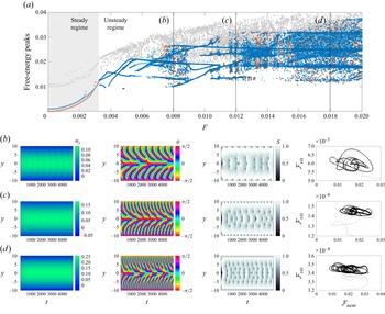
 F
F S=1
S=1 −
− +
+ F=0.008,0.012,0.018
 C=0.1
C=0.1 K=0.01
 L=20
L=20 λ=0
λ=0 U
U F
F Re∈[0,35]
 Er∈[0,2000]
 Pe∈[0,0.6]
 ϵ=0.001
 F=0.0024
 x
x F=0.006
 x=50
x=50 U
U F
F Re∈[0,18]
 Er∈[0,1000]
 Pe∈[0,0.3]
 ϵ=0.001
 F=0.0014
 C=0.1
C=0.1 K=0.01
 L=20
L=20 λ=0.2
λ=0.2 C=0.1
C=0.1 K=0.01
 L=20
L=20 λ=1
λ=1 C=0.1
C=0.1 K=0.1
K=0.1 L=20
L=20 λ=0
λ=0 Fnem
Fnem F
F


 Open access

