


1. Introduction
Drag reduction in turbulent flows can be achieved by introducing a thin lubricating layer near the wall, which reduces frictional losses (Joseph et al. Reference Joseph, Bai, Chen and Renardy1997). This strategy has been extensively studied through experiments and has found industrial applications, particularly in the transport of crude oil through pipelines (Isaac & Speed Reference Isaac and Speed1904; Looman Reference Looman1916; Joseph et al. Reference Joseph, Renardy and Renardy1984, Reference Joseph, Bai, Chen and Renardy1997; Hu & Joseph Reference Hu and Joseph1989). Another widely explored approach to drag reduction involves the addition of polymeric additives, which alter the rheological behaviour of the fluid and lead to significant friction reduction (Forrest & Grierson Reference Forrest and Grierson1931; Virk Reference Virk1975; White & Mungal Reference White and Mungal2008; Wang et al. Reference Wang, Yu, Zakin and Shi2011). In this study, we aim to combine these two mechanisms by employing a non-Newtonian lubricating layer to facilitate the flow of a Newtonian core fluid.
Beyond its industrial relevance, this configuration is also relevant in biomedical contexts, such as the human respiratory tract, where a thin mucus layer – characterised by viscoelastic and shear-thinning properties – modulates airflow resistance (Fontanari et al. Reference Fontanari, Zattara-Hartmann, Burnet and Jammes1997; Sue-Chu Reference Sue-Chu2012; Fazla et al. Reference Fazla, Erken, Izbassarov, Romanò, Grotberg and Muradoglu2024). While not the main focus of this study, such parallels highlight the broader relevance of understanding how non-Newtonian lubricating films interact with turbulent flows under the influence of surface tension.
Despite their practical importance, multiphase flows involving non-Newtonian fluids have received relatively limited attention. While a substantial body of work exists on single-phase non-Newtonian laminar and turbulent flows (Arosemena, Andersson & Solsvik Reference Arosemena, Andersson and Solsvik2021; Amor et al. Reference Amor, Soligo, Mazzino and Rosti2024; Serafini et al. Reference Serafini, Battista, Gualtieri and Casciola2024; Milocco et al. Reference Milocco, Giamagas, Zonta and Soldati2025; Rosti Reference Rosti2025; Xu et al. Reference Xu, Zhang, Brandt, Song and Shishkina2025), far fewer studies have addressed multiphase systems. Several works have focused on the motion of rigid particles – both spherical and non-spherical – in non-Newtonian fluids (D’Avino et al. Reference D’Avino, Greco and Maffettone2017; Lu et al. Reference Lu, Liu, Hu and Xuan2017; Datt & Elfring Reference Datt and Elfring2018; Zenit & Feng Reference Zenit and Feng2018; Hu et al. Reference Hu, Yu, Atomsa and Zhao2024; Habibi et al. Reference Habibi, Iqbal, Ardekani, Chaparian, Brandt and Tammisola2025). However, when gas–liquid or liquid–liquid systems are considered, the literature is sparse, particularly regarding interface-resolved simulations. Most studies in this area have examined the dynamics, deformation and interaction of drops and bubbles in non-Newtonian fluids, and vice versa (Oishi et al. Reference Oishi, Martins, Tomé and Alves2012; Yue & Feng Reference Yue and Feng2012; Wang, Do-Quang & Amberg Reference Wang, Do-Quang and Amberg2017; Amani et al. Reference Amani, Balcázar, Castro and Oliva2019; Balasubramanian et al. Reference Balasubramanian, Sanjay, Jalaal, Vinuesa and Tammisola2024), with only a small number investigating turbulent conditions using interface-resolved simulations (Rosti & Brandt Reference Rosti and Brandt2017; Del Gaudio et al. Reference Del Gaudio, Constantinescu, Di Cristo, De Paola and Vacca2024).
We address this problem through direct numerical simulations (DNS) of a turbulent channel flow at shear Reynolds number $\textit{Re}_\tau = 300$
, driven by a constant mean pressure gradient. The domain contains a thin lubricating layer near the bottom wall, separated from the Newtonian bulk by a deformable interface governed by surface tension, with a fixed Weber number
$\textit{Re}_\tau = 300$
, driven by a constant mean pressure gradient. The domain contains a thin lubricating layer near the bottom wall, separated from the Newtonian bulk by a deformable interface governed by surface tension, with a fixed Weber number $\textit{We} = 0.5$
. All cases assume density-matched fluids to isolate rheological effects from buoyancy or inertial stratification. We consider a reference single-phase Newtonian case, alongside four two-layer configurations in which the lubricating layer exhibits increasing rheological complexity: (i) Newtonian; (ii) shear-thinning described by a Carreau model; (iii) shear-thinning and viscoelasticity combined via a FENE-P model; and (iv) purely viscoelastic behaviour modelled by FENE-CR. In all cases, the zero-shear viscosity of the lubricating layer is matched to that of the core fluid to allow meaningful comparison. Such fluids occur in real-world applications and can also be engineered by incorporating micro-structures into light oils or other fluids (Ewoldt & Saengow Reference Ewoldt and Saengow2022). In line with previous findings for Newtonian–Newtonian fluids (Roccon, Zonta & Soldati Reference Roccon, Zonta and Soldati2019), surface tension alone contributes substantially to drag reduction. However, the presence of shear-thinning behaviour without elasticity does not significantly enhance this effect: the Carreau fluid, despite its reduced apparent viscosity near the wall, yields drag reduction levels comparable to the Newtonian case. In contrast, viscoelastic effects play a decisive role, and both FENE-P and FENE-CR fluids lead to drag reduction, highlighting the importance of the elastic component in modifying interfacial dynamics and turbulence structure.
$\textit{We} = 0.5$
. All cases assume density-matched fluids to isolate rheological effects from buoyancy or inertial stratification. We consider a reference single-phase Newtonian case, alongside four two-layer configurations in which the lubricating layer exhibits increasing rheological complexity: (i) Newtonian; (ii) shear-thinning described by a Carreau model; (iii) shear-thinning and viscoelasticity combined via a FENE-P model; and (iv) purely viscoelastic behaviour modelled by FENE-CR. In all cases, the zero-shear viscosity of the lubricating layer is matched to that of the core fluid to allow meaningful comparison. Such fluids occur in real-world applications and can also be engineered by incorporating micro-structures into light oils or other fluids (Ewoldt & Saengow Reference Ewoldt and Saengow2022). In line with previous findings for Newtonian–Newtonian fluids (Roccon, Zonta & Soldati Reference Roccon, Zonta and Soldati2019), surface tension alone contributes substantially to drag reduction. However, the presence of shear-thinning behaviour without elasticity does not significantly enhance this effect: the Carreau fluid, despite its reduced apparent viscosity near the wall, yields drag reduction levels comparable to the Newtonian case. In contrast, viscoelastic effects play a decisive role, and both FENE-P and FENE-CR fluids lead to drag reduction, highlighting the importance of the elastic component in modifying interfacial dynamics and turbulence structure.
2. Methodology
We consider a channel flow with a main Newtonian fluid layer (thickness $1.7h$
) lubricated by a thin non-Newtonian layer (thickness
$1.7h$
) lubricated by a thin non-Newtonian layer (thickness $0.3h$
), as depicted in figure 1. The channel has dimensions
$0.3h$
), as depicted in figure 1. The channel has dimensions $L_{x} \times L_{y} \times L_{z} = 4\pi h \times 2\pi h \times 2h$
, where
$L_{x} \times L_{y} \times L_{z} = 4\pi h \times 2\pi h \times 2h$
, where $h$
is the channel half-height, and
$h$
is the channel half-height, and $x$
,
$x$
, $y$
,
$y$
, $z$
are the streamwise, spanwise and wall-normal directions, respectively. The two fluids have equal density,
$z$
are the streamwise, spanwise and wall-normal directions, respectively. The two fluids have equal density, $\rho _m = \rho _l = \rho$
, and are separated by a deformable interface characterised by a constant surface tension
$\rho _m = \rho _l = \rho$
, and are separated by a deformable interface characterised by a constant surface tension $\sigma$
. The DNS of the Navier–Stokes equations coupled with a Cahn–Hilliard equation are used to describe the dynamics of the two-phase flow (Jacqmin Reference Jacqmin1999; Roccon, Zonta & Soldati Reference Roccon, Zonta and Soldati2023). An additional transport equation for the conformation tensor is solved when viscoelastic fluids are considered.
$\sigma$
. The DNS of the Navier–Stokes equations coupled with a Cahn–Hilliard equation are used to describe the dynamics of the two-phase flow (Jacqmin Reference Jacqmin1999; Roccon, Zonta & Soldati Reference Roccon, Zonta and Soldati2023). An additional transport equation for the conformation tensor is solved when viscoelastic fluids are considered.
Sketch of the simulation set-up considered. The flow of a main Newtonian layer having nominal thickness $1.7h$
is favoured by a non-Newtonian lubricating layer having nominal thickness
$1.7h$
is favoured by a non-Newtonian lubricating layer having nominal thickness $0.3h$
. The two fluids are immiscible and separated by a deformable interface; the flow is driven by a constant pressure gradient along the streamwise direction. The case shown refers to a FENE-CR lubricating layer and the colour map (yellow for low, violet for high) shows the
$0.3h$
. The two fluids are immiscible and separated by a deformable interface; the flow is driven by a constant pressure gradient along the streamwise direction. The case shown refers to a FENE-CR lubricating layer and the colour map (yellow for low, violet for high) shows the $x{-}z$
component of the polymer stress tensor.
$x{-}z$
component of the polymer stress tensor.

2.1. Phase-field method
The phase-field method employs a diffuse-interface formulation in which the sharp boundary between immiscible fluids is replaced by a thin transition layer, across which fluid properties vary continuously. This is achieved by introducing the phase-field variable $\phi$
, which is an indicator function:
$\phi$
, which is an indicator function: $\phi = 1$
in the main layer, and
$\phi = 1$
in the main layer, and $\phi = -1$
in the lubricating layer. The fluid interface is then represented by the region where
$\phi = -1$
in the lubricating layer. The fluid interface is then represented by the region where $\phi$
varies smoothly between these two values. The distribution and dynamics of
$\phi$
varies smoothly between these two values. The distribution and dynamics of $\phi$
are governed by the dimensionless Cahn–Hilliard equation:
$\phi$
are governed by the dimensionless Cahn–Hilliard equation:
 \begin{equation} \frac {\partial \phi }{\partial t} + \boldsymbol{u} \boldsymbol{\cdot }\boldsymbol{\nabla }\phi = \frac {1}{\textit{Pe}}\, {\nabla} ^2\! \mu _{\phi } , \end{equation}
where $\textit{Pe} = u_\tau h/\mathcal{M}\beta$
is the Péclet number, i.e. the ratio between the convective and diffusive time scales of the interface. Here,
$\textit{Pe} = u_\tau h/\mathcal{M}\beta$
is the Péclet number, i.e. the ratio between the convective and diffusive time scales of the interface. Here, $u_\tau$
denotes the friction velocity,
$u_\tau$
denotes the friction velocity, $h$
is the channel half-height,
$h$
is the channel half-height, $\mathcal{M}$
is the mobility, and
$\mathcal{M}$
is the mobility, and $\beta$
is a positive constant. The chemical potential
$\beta$
is a positive constant. The chemical potential $\mu _{\phi }$
is defined as the variational derivative of a Ginzburg–Landau free-energy functional:
$\mu _{\phi }$
is defined as the variational derivative of a Ginzburg–Landau free-energy functional:
 \begin{equation} \mu _{\phi } = \frac {\delta \mathcal{F}\,[\phi ,\boldsymbol{\nabla }\phi ]}{\delta \phi }. \end{equation}
We consider a system composed by two immiscible fluids, one of which is viscoelastic. The corresponding Ginzburg–Landau free-energy functional can be expressed as the sum of three different contributions, namely a bulk term, an interfacial (or mixing) term, and an elastic contribution (Yue et al. Reference Yue, Feng, Liu and Shen2004):
 \begin{equation} \mathcal{F}\,[\phi , \boldsymbol{\nabla }\phi ] = \int _{\varOmega } \bigl(f_0(\phi ) + f_{\textit{mix}}(\boldsymbol{\nabla }\phi ) + f_e(\phi )\bigr)\, \textrm{d}\varOmega , \end{equation}
with
 \begin{align} f_0(\phi ) = \frac {(\phi ^2-1)^2}{4}, \end{align}
 \begin{align} f_{\textit{mix}}(\boldsymbol{\nabla }\phi ) = \frac {\textit{Ch}^2}{2} |\boldsymbol{\nabla }\phi |^2, \end{align}
 \begin{align} f_e(\phi ) = \frac {1-\phi }{2}\,\frac {1-x_0}{\textit{Wi}_\tau } \int _{\mathbb{R}^3} \psi \left ( \ln \psi + \frac {1}{2} \boldsymbol{q} \boldsymbol{\cdot }\boldsymbol{q} \right ) \textrm{d}\boldsymbol{q}, \end{align}
where $f_0$
represents the bulk free energy driving phase separation,
$f_0$
represents the bulk free energy driving phase separation, $f_{\textit{mix}}$
accounts for the interfacial energy, which is proportional to the Cahn number
$f_{\textit{mix}}$
accounts for the interfacial energy, which is proportional to the Cahn number $\textit{Ch}=\xi /h$
(ratio of interface thickness
$\textit{Ch}=\xi /h$
(ratio of interface thickness $\xi$
to channel half-height
$\xi$
to channel half-height $h$
), and
$h$
), and $f_e$
models the elastic contribution associated with polymer deformation. Here,
$f_e$
models the elastic contribution associated with polymer deformation. Here, $\psi$
denotes the normalised probability distribution function of the polymer end-to-end vector
$\psi$
denotes the normalised probability distribution function of the polymer end-to-end vector $\boldsymbol{q}$
(i.e.
$\boldsymbol{q}$
(i.e. $\int _{\mathbb{R}^3} \psi \, \textrm{d}\boldsymbol{q} =1$
) (Bird, Armstrong & Hassager Reference Bird, Armstrong and Hassager1987). The phase-field formulation implicitly captures topological changes of the interface, such as rupture events, while preserving smooth transitions. From (2.2), the chemical potential is obtained as
$\int _{\mathbb{R}^3} \psi \, \textrm{d}\boldsymbol{q} =1$
) (Bird, Armstrong & Hassager Reference Bird, Armstrong and Hassager1987). The phase-field formulation implicitly captures topological changes of the interface, such as rupture events, while preserving smooth transitions. From (2.2), the chemical potential is obtained as
 \begin{equation} \mu _{\phi } = \phi ^3 - \phi - \textit{Ch}^2\, {\nabla} ^2 \phi + \frac {\delta f_e}{\delta \phi }. \end{equation}
Following Yue et al. (Reference Yue, Feng, Liu and Shen2004, Reference Yue, Feng, Liu and Shen2005), the elastic contribution $\delta f_e/\delta \phi$
becomes negligible in the sharp-interface limit. The governing Cahn–Hilliard equation then reduces to
$\delta f_e/\delta \phi$
becomes negligible in the sharp-interface limit. The governing Cahn–Hilliard equation then reduces to
 \begin{equation} \frac {\partial \phi }{\partial t} + \boldsymbol{u} \boldsymbol{\cdot }\boldsymbol{\nabla }\phi = \frac {1}{\textit{Pe}}\, {\nabla} ^2 \big (\phi ^3 - \phi - \textit{Ch}^2\, {\nabla} ^2 \phi \big ). \end{equation}
2.2. Hydrodynamics
To describe the hydrodynamics of the two-phase system, the Cahn–Hilliard equation is coupled with the Navier–Stokes equations within the one-fluid formulation (Prosperetti & Tryggvason Reference Prosperetti and Tryggvason2007). The presence of a deformable interface is accounted for by an additional source term representing surface tension forces. This formulation ensures continuity of velocity and stresses across the interface (Landau & Lifshitz Reference Landau and Lifshitz1987; Panton Reference Panton2013). The resulting dimensionless governing equations read as
 \begin{equation} \boldsymbol{\nabla } \boldsymbol{\cdot } \boldsymbol{u} = 0, \\[-12pt] \nonumber \end{equation}
 \begin{equation} \frac {\partial \boldsymbol{u}}{\partial t} + \boldsymbol{u} \boldsymbol{\cdot } \boldsymbol{\nabla \!} \boldsymbol{u} = -\boldsymbol{\nabla \!} p + \frac {1}{\textit{Re}_\tau }\, \boldsymbol{\nabla } \boldsymbol{\cdot } \boldsymbol{\tau }_k + \frac {3\,\textit{Ch}}{\sqrt {8}\, \textit{We}}\, \boldsymbol{\nabla } \boldsymbol{\cdot } \boldsymbol{\tau }_c, \end{equation}
where $\boldsymbol{u}=(u,v,w)$
is the velocity vector and
$\boldsymbol{u}=(u,v,w)$
is the velocity vector and $\boldsymbol{\nabla \!} p$
is the pressure gradient. The last term in (2.10) represents the contribution of the surface tension forces where the corresponding stress tensor is defined as
$\boldsymbol{\nabla \!} p$
is the pressure gradient. The last term in (2.10) represents the contribution of the surface tension forces where the corresponding stress tensor is defined as $\boldsymbol{\tau }_c=|\boldsymbol{\nabla }\phi |^2 \boldsymbol{I} - \boldsymbol{\nabla }\phi \otimes \boldsymbol{\nabla }\phi$
, in accordance with the Korteweg formulation (Korteweg Reference Korteweg1901). The dimensionless parameters are the shear Reynolds number
$\boldsymbol{\tau }_c=|\boldsymbol{\nabla }\phi |^2 \boldsymbol{I} - \boldsymbol{\nabla }\phi \otimes \boldsymbol{\nabla }\phi$
, in accordance with the Korteweg formulation (Korteweg Reference Korteweg1901). The dimensionless parameters are the shear Reynolds number $\textit{Re}_{\tau }= \rho u_\tau h/\mu _m$
, based on the Newtonian fluid viscosity, and the Weber number
$\textit{Re}_{\tau }= \rho u_\tau h/\mu _m$
, based on the Newtonian fluid viscosity, and the Weber number $\textit{We}=\rho u^2_\tau h /\sigma$
, i.e. the ratio between inertial and surface tension forces.
$\textit{We}=\rho u^2_\tau h /\sigma$
, i.e. the ratio between inertial and surface tension forces.
2.3. Non-Newtonian rheology
The rheological behaviour of the lubricating layer is controlled by the constitutive stress tensor, $\boldsymbol{\tau }_k$
. In addition to a reference Newtonian lubricating layer, we consider the following non-Newtonian models: (i) Carreau model, representative of a shear-thinning fluid; (ii) FENE-P model, a viscoelastic and shear-thinning fluid; and (iii) FENE-CR model, a viscoelastic fluid characterised by uniform viscosity. Hence for the different cases considered, the constitutive stress tensor
$\boldsymbol{\tau }_k$
. In addition to a reference Newtonian lubricating layer, we consider the following non-Newtonian models: (i) Carreau model, representative of a shear-thinning fluid; (ii) FENE-P model, a viscoelastic and shear-thinning fluid; and (iii) FENE-CR model, a viscoelastic fluid characterised by uniform viscosity. Hence for the different cases considered, the constitutive stress tensor $\boldsymbol{\tau }_k$
is defined as
$\boldsymbol{\tau }_k$
is defined as
 \begin{equation} \boldsymbol{\tau }_k = \begin{cases} \left (\boldsymbol{\nabla \!} \boldsymbol{u} + \boldsymbol{\nabla \!} \boldsymbol{u}^{\mathrm{T}}\right ), & \text{Newtonian},\\[6pt] \left (1+\dfrac {1-\phi}{2}\left (\beta ( \dot {\gamma }) - 1\right )\right ) \left (\boldsymbol{\nabla \!} \boldsymbol{u} + \boldsymbol{\nabla \!} \boldsymbol{u}^{\mathrm{T}}\right ), & \text{Carreau},\\[6pt] x_0 \left (1+\dfrac {(1/x_0-1)(\phi +1)}{2}\right ) \left (\boldsymbol{\nabla \!} \boldsymbol{u} + \boldsymbol{\nabla \!} \boldsymbol{u}^{\mathrm{T}}\right ) + (1-x_0)\, \boldsymbol{\tau }_{\!p}, & \text{FENE-P and FENE-CR}. \end{cases} \end{equation}
For the shear-thinning Carreau model (Carreau Reference Carreau1972), the effective non-dimensional viscosity is expressed through the relation
 \begin{equation} \beta (\dot {\gamma })= \frac {\mu _l(\dot \gamma )}{\mu _0} = \frac {\mu _\infty }{\mu _0} + \left (1 - \frac {\mu _\infty }{\mu _0}\right ) \left [1 + (\mathit{Cu}\, \dot {\gamma })^2 \right ]^{(n-1)/2}, \end{equation}
where $\mu _\infty /\mu _0$
is the infinite-strain to zero-strain viscosity ratio,
$\mu _\infty /\mu _0$
is the infinite-strain to zero-strain viscosity ratio, $\mathit{Cu} = \varLambda u_\tau / h$
is the Carreau number, with
$\mathit{Cu} = \varLambda u_\tau / h$
is the Carreau number, with $\varLambda$
the fluid characteristic time scale,
$\varLambda$
the fluid characteristic time scale, $n$
is the flow behaviour index, and
$n$
is the flow behaviour index, and $\dot {\gamma }$
is the strain rate. The latter is defined as
$\dot {\gamma }$
is the strain rate. The latter is defined as $\dot {\gamma } = \sqrt {2\, \boldsymbol{S}\boldsymbol{S}}$
, with
$\dot {\gamma } = \sqrt {2\, \boldsymbol{S}\boldsymbol{S}}$
, with $\boldsymbol{S} = 1/2 (\boldsymbol{\nabla \!} \boldsymbol{u} + \boldsymbol{\nabla \!} \boldsymbol{u}^{{\rm T}} )$
.
$\boldsymbol{S} = 1/2 (\boldsymbol{\nabla \!} \boldsymbol{u} + \boldsymbol{\nabla \!} \boldsymbol{u}^{{\rm T}} )$
.
For the viscoelastic cases (FENE-P and FENE-CR), the viscosity ratio $x_0 = \mu _s/(\mu _s + \mu _p)$
quantifies the solvent contribution to the total zero-strain viscosity
$x_0 = \mu _s/(\mu _s + \mu _p)$
quantifies the solvent contribution to the total zero-strain viscosity $\mu _0 = \mu _s+\mu _p=\mu _m$
, and has been set equal to the top Newtonian layer. The polymer stress tensor is defined as
$\mu _0 = \mu _s+\mu _p=\mu _m$
, and has been set equal to the top Newtonian layer. The polymer stress tensor is defined as
 \begin{equation} \boldsymbol{\tau }_{\!p} = \frac {\textit{Re}_\tau }{\mathit{Wi}_\tau } \left (f(\boldsymbol{C})\, \boldsymbol{C} - g(\boldsymbol{C})\, \boldsymbol{I}\right ), \end{equation}
where $\mathit{Wi}_\tau = \rho \lambda u^2_\tau /\mu _0$
is the shear Weissenberg number, while
$\mathit{Wi}_\tau = \rho \lambda u^2_\tau /\mu _0$
is the shear Weissenberg number, while $\textit{Wi}= \mathit{Wi}_\tau /\textit{Re}_\tau$
is the Weissenberg number (coincident with the Deborah number), i.e. the ratio of elastic to flow time scale, and
$\textit{Wi}= \mathit{Wi}_\tau /\textit{Re}_\tau$
is the Weissenberg number (coincident with the Deborah number), i.e. the ratio of elastic to flow time scale, and $\lambda$
is the polymer relaxation time. The conformation tensor
$\lambda$
is the polymer relaxation time. The conformation tensor $\boldsymbol{C}$
describes the polymer microstructure and is described by the equation (Alves, Oliveira & Pinho Reference Alves, Oliveira and Pinho2021)
$\boldsymbol{C}$
describes the polymer microstructure and is described by the equation (Alves, Oliveira & Pinho Reference Alves, Oliveira and Pinho2021)
 \begin{align} \frac {\partial \boldsymbol{C}}{\partial t} + \boldsymbol{u} \boldsymbol{\cdot } \boldsymbol{\nabla \!} \boldsymbol{C} = \boldsymbol{C} \boldsymbol{\cdot } \boldsymbol{\nabla \!} \boldsymbol{u} + \left (\boldsymbol{C} \boldsymbol{\cdot } \boldsymbol{\nabla \!} \boldsymbol{u}\right )^{{\rm T}} - \frac {1-\phi }{2\,\mathit{Wi}}\left [f(\boldsymbol{C})\, \boldsymbol{C} - g(\boldsymbol{C})\, \boldsymbol{I}\right ] + \frac {1}{\textit{Re}_{\tau }\, \mathit{Sc}_p}\, {\nabla} ^2 \boldsymbol{C}, \end{align}
where $\mathit{Sc}_p = \mu _0/(\rho k)$
is the Schmidt number controlling the magnitude of the diffusive regularisation term for the polymer. The finite polymer extensibility is captured by
$\mathit{Sc}_p = \mu _0/(\rho k)$
is the Schmidt number controlling the magnitude of the diffusive regularisation term for the polymer. The finite polymer extensibility is captured by $f(\boldsymbol{C})=L^2/(L^2-\mathrm{tr}(\boldsymbol{C}))$
, with
$f(\boldsymbol{C})=L^2/(L^2-\mathrm{tr}(\boldsymbol{C}))$
, with $L$
the extensibility limit. The choice of
$L$
the extensibility limit. The choice of $g(\boldsymbol{C})$
distinguishes the models:
$g(\boldsymbol{C})$
distinguishes the models: $g=1$
gives the FENE-P model, which accounts also for shear-thinning effects (Bird et al. Reference Bird, Armstrong and Hassager1987), while
$g=1$
gives the FENE-P model, which accounts also for shear-thinning effects (Bird et al. Reference Bird, Armstrong and Hassager1987), while $g=f(\boldsymbol{C})$
yields the purely viscoelastic FENE-CR model (Chilcott & Rallison Reference Chilcott and Rallison1988). Notably, the formulation employed here ensures a consistent transition between different rheological behaviours. In the Newtonian region (
$g=f(\boldsymbol{C})$
yields the purely viscoelastic FENE-CR model (Chilcott & Rallison Reference Chilcott and Rallison1988). Notably, the formulation employed here ensures a consistent transition between different rheological behaviours. In the Newtonian region ( $\phi \to 1$
), the effective Weissenberg number
$\phi \to 1$
), the effective Weissenberg number $\mathit{Wi}(\phi )=(1-\phi )/2\, \textit{Wi}$
tends to zero, the relaxation term vanishes, and the conformation tensor reduces to
$\mathit{Wi}(\phi )=(1-\phi )/2\, \textit{Wi}$
tends to zero, the relaxation term vanishes, and the conformation tensor reduces to $\boldsymbol{C} \approx \boldsymbol{I}$
. The polymer stress contribution therefore becomes negligible, and the standard Navier–Stokes equations are recovered. In contrast, in the viscoelastic region (
$\boldsymbol{C} \approx \boldsymbol{I}$
. The polymer stress contribution therefore becomes negligible, and the standard Navier–Stokes equations are recovered. In contrast, in the viscoelastic region ( $\phi \to -1$
), the full polymer stress is active, introducing both elasticity and shear-thinning effects, depending on the chosen closure.
$\phi \to -1$
), the full polymer stress is active, introducing both elasticity and shear-thinning effects, depending on the chosen closure.
2.4. Numerical method
The governing equations (2.8), (2.9), (2.10) and (2.14) are solved using FLOW36, an open-source GPU-ready spectral solver (Roccon, Soligo & Soldati Reference Roccon, Soligo and Soldati2025). Spatial discretisation relies on Fourier expansions in the two homogeneous directions ( $x$
,
$x$
, $y$
) and Chebyshev polynomials in the wall-normal direction (
$y$
) and Chebyshev polynomials in the wall-normal direction ( $z$
).
$z$
).
The Navier–Stokes equations are solved in the wall-normal velocity–vorticity formulation (Kim, Moin & Moser Reference Kim, Moin and Moser1987; Speziale Reference Speziale1987), which yields a fourth-order equation for the wall-normal velocity $w$
, and a second-order equation for the wall-normal vorticity
$w$
, and a second-order equation for the wall-normal vorticity $\omega _z$
. The phase-field equation (2.8) is reformulated as two coupled second-order equations (Badalassi, Ceniceros & Banerjee Reference Badalassi, Ceniceros and Banerjee2003). Time advancement of both the momentum and phase-field equations employs an implicit–explicit scheme (Moin & Kim Reference Moin and Kim1980): linear terms are integrated implicitly (Crank–Nicolson for the Navier–Stokes equations, backward Euler for the phase-field; Yue et al. Reference Yue, Feng, Liu and Shen2004), while nonlinear terms are treated explicitly using a second-order Adams–Bashforth method.
$\omega _z$
. The phase-field equation (2.8) is reformulated as two coupled second-order equations (Badalassi, Ceniceros & Banerjee Reference Badalassi, Ceniceros and Banerjee2003). Time advancement of both the momentum and phase-field equations employs an implicit–explicit scheme (Moin & Kim Reference Moin and Kim1980): linear terms are integrated implicitly (Crank–Nicolson for the Navier–Stokes equations, backward Euler for the phase-field; Yue et al. Reference Yue, Feng, Liu and Shen2004), while nonlinear terms are treated explicitly using a second-order Adams–Bashforth method.
For viscoelastic simulations (FENE-P, FENE-CR), the conformation tensor equation is advanced in time simultaneously with the momentum and phase-field equations. The numerical treatment of the conformation tensor is particularly delicate, as the loss of positive-definiteness and the development of steep polymer stress gradients near the walls may trigger numerical instabilities. To alleviate these issues, a diffusive regularisation term for the polymer $(\mathit{Re}_{\tau }\, \mathit{\textit{Sc}_{\!p}})^{-1}\, {\nabla} ^2 \boldsymbol{C}$
is introduced following standard practice in pseudo-spectral simulations (Sureshkumar, Beris & Handler Reference Sureshkumar, Beris and Handler1997; Dimitropoulos, Sureshkumar & Beris Reference Dimitropoulos, Sureshkumar and Beris1998; Xi & Graham Reference Xi and Graham2010). The diffusive contribution in the conformation tensor equation is discretised implicitly via a Crank–Nicolson scheme, while the nonlinear terms are advanced explicitly with a second-order Adams–Bashforth scheme. To ensure the boundedness of the conformation tensor
$(\mathit{Re}_{\tau }\, \mathit{\textit{Sc}_{\!p}})^{-1}\, {\nabla} ^2 \boldsymbol{C}$
is introduced following standard practice in pseudo-spectral simulations (Sureshkumar, Beris & Handler Reference Sureshkumar, Beris and Handler1997; Dimitropoulos, Sureshkumar & Beris Reference Dimitropoulos, Sureshkumar and Beris1998; Xi & Graham Reference Xi and Graham2010). The diffusive contribution in the conformation tensor equation is discretised implicitly via a Crank–Nicolson scheme, while the nonlinear terms are advanced explicitly with a second-order Adams–Bashforth scheme. To ensure the boundedness of the conformation tensor $\boldsymbol{C}$
, i.e.
$\boldsymbol{C}$
, i.e. $\operatorname {tr}(\boldsymbol{C}) \lt L^2$
, we adopt the stabilisation technique proposed by Vaithianathan & Collins (Reference Vaithianathan and Collins2003) and later refined by Dubief et al. (Reference Dubief, Terrapon, White, Shaqfeh, Moin and Lele2005) and Richter, Iaccarino & Shaqfeh (Reference Richter, Iaccarino and Shaqfeh2010). This method enforces the boundedness of
$\operatorname {tr}(\boldsymbol{C}) \lt L^2$
, we adopt the stabilisation technique proposed by Vaithianathan & Collins (Reference Vaithianathan and Collins2003) and later refined by Dubief et al. (Reference Dubief, Terrapon, White, Shaqfeh, Moin and Lele2005) and Richter, Iaccarino & Shaqfeh (Reference Richter, Iaccarino and Shaqfeh2010). This method enforces the boundedness of $\operatorname {tr}(\boldsymbol{C})$
by evolving an auxiliary variable
$\operatorname {tr}(\boldsymbol{C})$
by evolving an auxiliary variable $f^{-1} = 1 - \operatorname {tr}(\boldsymbol{C})/L^2$
for the FENE-P model (or
$f^{-1} = 1 - \operatorname {tr}(\boldsymbol{C})/L^2$
for the FENE-P model (or $f$
in the FENE-CR case) instead of
$f$
in the FENE-CR case) instead of $\boldsymbol{C}$
directly. In both formulations, the resulting value of
$\boldsymbol{C}$
directly. In both formulations, the resulting value of $f^{-1}$
(or
$f^{-1}$
(or $f$
) is held fixed while the nonlinear terms of conformation tensor
$f$
) is held fixed while the nonlinear terms of conformation tensor $\boldsymbol{C}$
are computed, ensuring that
$\boldsymbol{C}$
are computed, ensuring that $\operatorname {tr}(\boldsymbol{C}) \leqslant L^2$
at all times, and maintaining numerical stability.
$\operatorname {tr}(\boldsymbol{C}) \leqslant L^2$
at all times, and maintaining numerical stability.
2.5. Boundary conditions
Periodic boundary conditions are applied along the two homogeneous directions ( $x$
and
$x$
and $y$
), where Fourier transforms are employed. At the walls (
$y$
), where Fourier transforms are employed. At the walls ( $z/h = \pm 1$
), no-slip boundary conditions are enforced for the velocity field:
$z/h = \pm 1$
), no-slip boundary conditions are enforced for the velocity field:
 \begin{equation} \boldsymbol{u}(z/h = \pm 1) = 0. \end{equation}
Using the wall-normal velocity–vorticity formulation, the corresponding conditions for the wall-normal velocity $w$
and vorticity
$w$
and vorticity $\omega _z$
can be derived by combining the no-slip condition with the continuity equation. Specifically, for the wall-normal velocity we have
$\omega _z$
can be derived by combining the no-slip condition with the continuity equation. Specifically, for the wall-normal velocity we have
 \begin{equation} w(z/h = \pm 1) = 0, \quad \frac {\partial w}{\partial z}\Big |_{z/h = \pm 1} = 0, \end{equation}
and for the wall-normal vorticity we have
 \begin{equation} \omega _z(z/h = \pm 1) = \frac {\partial v}{\partial x}\Big |_{z/h = \pm 1} - \frac {\partial u}{\partial y}\Big |_{z/h = \pm 1} = 0. \end{equation}
The Cahn–Hilliard equation is solved by imposing no-flux conditions for the phase-field variable and the chemical potential at the two walls:
 \begin{equation} \frac {\partial \phi }{\partial z}\Big |_{z/h = \pm 1} = 0,\quad \frac {\partial \mu _\phi }{\partial z}\Big |_{z/h = \pm 1} = 0. \end{equation}
From a mathematical point of view, this is equivalent to imposing the boundary conditions (Jacqmin Reference Jacqmin1999; Yue et al. Reference Yue, Feng, Liu and Shen2004)
 \begin{equation} \frac {\partial \phi }{\partial z}\Big |_{z/h = \pm 1} = 0,\quad \frac {\partial ^3 \phi }{\partial z^3}\Big |_{z/h = \pm 1} = 0. \end{equation}
These conditions ensure global conservation of the phase field:
 \begin{equation} \frac {\mathrm{d}}{\mathrm{d}t} \int _\varOmega \phi \, \mathrm{d}\varOmega = 0, \end{equation}
where $\varOmega$
is the computational domain. While this guarantees mass conservation of the entire system, it does not strictly enforce mass conservation of each phase (
$\varOmega$
is the computational domain. While this guarantees mass conservation of the entire system, it does not strictly enforce mass conservation of each phase ( $\phi = +1$
and
$\phi = +1$
and $\phi = -1$
), and small leakages between phases may occur (Yue, Zhou & Feng Reference Yue, Zhou and Feng2007; Soligo, Roccon & Soldati Reference Soligo, Roccon and Soldati2019). In the present simulations, mass leakage is always below 1 %. For the conformation tensor, the boundary conditions are set according to the rheological properties of the respective layer. At the top wall (
$\phi = -1$
), and small leakages between phases may occur (Yue, Zhou & Feng Reference Yue, Zhou and Feng2007; Soligo, Roccon & Soldati Reference Soligo, Roccon and Soldati2019). In the present simulations, mass leakage is always below 1 %. For the conformation tensor, the boundary conditions are set according to the rheological properties of the respective layer. At the top wall ( $z/h=1$
), where the fluid is Newtonian, a Dirichlet condition corresponding to the coiled state of the polymers is imposed:
$z/h=1$
), where the fluid is Newtonian, a Dirichlet condition corresponding to the coiled state of the polymers is imposed:
 \begin{equation} \boldsymbol{C}|_{z/h=1} = \boldsymbol{I}. \end{equation}
At the bottom wall ( $z/h=-1$
), when a viscoelastic fluid layer is present (FENE-P or FENE-CR), zero artificial diffusivity is assumed (
$z/h=-1$
), when a viscoelastic fluid layer is present (FENE-P or FENE-CR), zero artificial diffusivity is assumed ( $Sc \to \infty$
), making the conformation tensor equation explicit at the wall (Dimitropoulos et al. Reference Dimitropoulos, Sureshkumar and Beris1998):
$Sc \to \infty$
), making the conformation tensor equation explicit at the wall (Dimitropoulos et al. Reference Dimitropoulos, Sureshkumar and Beris1998):
 \begin{equation} \boldsymbol{C}^{\,n+1}|_{z/h=-1} = \boldsymbol{C}^{\, n}|_{z/h=-1} + \frac {\Delta t}{2} \big ( 3 \boldsymbol{S}_c^{\, n}|_{z/h=-1} - \boldsymbol{S}_c^{\, n-1}|_{z/h=-1} \big ), \end{equation}
where $\boldsymbol{S}_c$
contains all nonlinear terms of the conformation tensor transport (2.14). This treatment ensures that the conformation tensor and the associated polymeric stress naturally follow the interface evolution and remain confined to the respective fluid layer.
$\boldsymbol{S}_c$
contains all nonlinear terms of the conformation tensor transport (2.14). This treatment ensures that the conformation tensor and the associated polymeric stress naturally follow the interface evolution and remain confined to the respective fluid layer.
2.6. Simulation set-up
We perform five sets of DNS of a turbulent channel flow. First, a precursor single-phase (SP) simulation at $\textit{Re}_\tau = 300$
is executed to reach a statistically steady state. The resulting flow field is then used to initialise the Newtonian simulation. All multiphase simulations are subsequently initialised from this stratified Newtonian configuration. The time step is maintained at
$\textit{Re}_\tau = 300$
is executed to reach a statistically steady state. The resulting flow field is then used to initialise the Newtonian simulation. All multiphase simulations are subsequently initialised from this stratified Newtonian configuration. The time step is maintained at $\Delta t^- = 0.25 \times 10^{-4}$
for all simulations.
$\Delta t^- = 0.25 \times 10^{-4}$
for all simulations.
The multiphase cases consider a main Newtonian layer above a thin lubricating layer, as illustrated in figure 1. The lubricating layer exhibits different rheological behaviour in each simulation: Newtonian, shear-thinning (Carreau model), viscoelastic and shear-thinning (FENE-P model), and purely viscoelastic (FENE-CR model). In all viscoelastic simulations, the Schmidt number is set to $\textit{Sc}_{\!p} = 1$
, chosen as a compromise to stabilise the numerical solution of the conformation tensor without significantly compromising physical fidelity (Sureshkumar & Beris Reference Sureshkumar and Beris1995). The chosen Schmidt number conforms to previous numerical studies (Xi & Graham Reference Xi and Graham2010; Zhu et al. Reference Zhu, Schrobsdorff, Schneider and Xi2018; Kelly et al. Reference Kelly, Goldstein, Burtsev, Suryanarayanan, Handler and Sonmez2025), and a sensitivity analysis of its effect is reported in Appendix A. For both viscoelastic simulations, the Weissenberg number is set to
$\textit{Sc}_{\!p} = 1$
, chosen as a compromise to stabilise the numerical solution of the conformation tensor without significantly compromising physical fidelity (Sureshkumar & Beris Reference Sureshkumar and Beris1995). The chosen Schmidt number conforms to previous numerical studies (Xi & Graham Reference Xi and Graham2010; Zhu et al. Reference Zhu, Schrobsdorff, Schneider and Xi2018; Kelly et al. Reference Kelly, Goldstein, Burtsev, Suryanarayanan, Handler and Sonmez2025), and a sensitivity analysis of its effect is reported in Appendix A. For both viscoelastic simulations, the Weissenberg number is set to $\mathit{Wi}_\tau = 50$
, and the viscosity ratio is set to
$\mathit{Wi}_\tau = 50$
, and the viscosity ratio is set to $x_0 = 0.9$
. In all cases, the zero-strain-rate viscosity of the lubricating layer is matched to that of the Newtonian upper layer,
$x_0 = 0.9$
. In all cases, the zero-strain-rate viscosity of the lubricating layer is matched to that of the Newtonian upper layer, $\mu _0 = \mu _m$
. The Carreau model parameters are tuned to reproduce the same degree of shear-thinning observed in the FENE-P simulation at
$\mu _0 = \mu _m$
. The Carreau model parameters are tuned to reproduce the same degree of shear-thinning observed in the FENE-P simulation at $\mathit{Wi}_\tau = 50$
and
$\mathit{Wi}_\tau = 50$
and $L = 30$
, using the known rheological response
$L = 30$
, using the known rheological response $\mu _l/\mu _0(\dot {\gamma }, x_0, \mathit{Wi}, L)$
as a reference (Tamano et al. Reference Tamano, Itoh, Hotta, Yokota and Morinishi2009), yielding
$\mu _l/\mu _0(\dot {\gamma }, x_0, \mathit{Wi}, L)$
as a reference (Tamano et al. Reference Tamano, Itoh, Hotta, Yokota and Morinishi2009), yielding $\mu _\infty /\mu _0 = 0.9$
,
$\mu _\infty /\mu _0 = 0.9$
, $\mathit{Cu} = 4$
and
$\mathit{Cu} = 4$
and $n = 0.45$
.
$n = 0.45$
.
For the SP, Newtonian and Carreau cases, a grid of $512 \times 256 \times 257$
points is used, whereas the viscoelastic simulations employ a finer grid of
$512 \times 256 \times 257$
points is used, whereas the viscoelastic simulations employ a finer grid of $512 \times 512 \times 513$
points to ensure numerical stability. To verify that this resolution is sufficient for the viscoelastic cases, we also performed additional simulations using a grid refined by a factor of 2 in all directions, and observed no appreciable differences. The surface tension of the liquid–liquid interface is constant for all cases and set via the Weber number
$512 \times 512 \times 513$
points to ensure numerical stability. To verify that this resolution is sufficient for the viscoelastic cases, we also performed additional simulations using a grid refined by a factor of 2 in all directions, and observed no appreciable differences. The surface tension of the liquid–liquid interface is constant for all cases and set via the Weber number $\textit{We} = 0.5$
. This value is consistent with our previous multiphase DNS database, and ensures that the interface remains compliant yet stable under turbulent forcing, in line with earlier studies on drag-reduced flows (Roccon et al. Reference Roccon, Zonta and Soldati2019, Reference Roccon, Zonta and Soldati2021, Reference Roccon, Zonta and Soldati2024). The Cahn number is set to
$\textit{We} = 0.5$
. This value is consistent with our previous multiphase DNS database, and ensures that the interface remains compliant yet stable under turbulent forcing, in line with earlier studies on drag-reduced flows (Roccon et al. Reference Roccon, Zonta and Soldati2019, Reference Roccon, Zonta and Soldati2021, Reference Roccon, Zonta and Soldati2024). The Cahn number is set to $\textit{Ch} = 0.02$
, and the Péclet number is computed as
$\textit{Ch} = 0.02$
, and the Péclet number is computed as $\textit{Pe} = 3/\textit{Ch}$
(Magaletti et al. Reference Magaletti, Picano, Chinappi, Marino and Casciola2013) to achieve asymptotic convergence to the sharp-interface limit. The interface is initially flat and located at
$\textit{Pe} = 3/\textit{Ch}$
(Magaletti et al. Reference Magaletti, Picano, Chinappi, Marino and Casciola2013) to achieve asymptotic convergence to the sharp-interface limit. The interface is initially flat and located at $h_l = 0.3h$
from the bottom wall. Specifically, the initial phase-field condition is
$h_l = 0.3h$
from the bottom wall. Specifically, the initial phase-field condition is
 \begin{equation} \phi (x/h, y/h, z/h) = -\tanh\! \left ( \frac {h_l/h-1 - z/h}{\sqrt {2}\, \textit{Ch}} \right )\!. \end{equation}
On the other hand, viscoelastic simulations are initialised with zero polymer stress, $\boldsymbol{\tau }_{\!p}=0$
, i.e.
$\boldsymbol{\tau }_{\!p}=0$
, i.e. $\boldsymbol{C}= \boldsymbol{I}$
in the entire domain. Given the prescribed boundaries condition on the conformation tensor, and because advective or stretching contributions in the Newtonian region do not develop due to the mild gradients of the conformation tensor, the latter remains constant over time.
$\boldsymbol{C}= \boldsymbol{I}$
in the entire domain. Given the prescribed boundaries condition on the conformation tensor, and because advective or stretching contributions in the Newtonian region do not develop due to the mild gradients of the conformation tensor, the latter remains constant over time.
3. Results
The drag reduction performance obtained from the different cases is first evaluated by looking at macroscopic flow parameters. Then the mean shear stress budget is used to obtain useful insights on the mechanisms leading to drag reduction, and in particular on the interplay between capillary action, shear-thinning and viscoelasticity. The statistics presented below have been computed once a new statistically steady-state configuration is attained for all configurations. All simulations exhibit an initial transient, whose duration depends on the specific case considered, where the flow adapts to the rheological properties of the lubricating layer. Once this new steady-state configuration is attained, statistics are computed using time window $\Delta t^+ = 4000$
.
$\Delta t^+ = 4000$
.
3.1. Mean flow and rheological features
Figure 2( $a$
) shows the rheology map of the lubricating fluids employed, where the dimensionless viscosity
$a$
) shows the rheology map of the lubricating fluids employed, where the dimensionless viscosity $\mu _l(\dot {\gamma })/\mu _0$
is shown as a function of the strain rate
$\mu _l(\dot {\gamma })/\mu _0$
is shown as a function of the strain rate $\dot {\gamma }$
. The shear-thinning region – where viscosity decreases with increasing strain rate – is the shaded grey area. The Carreau (green solid line) and FENE-P (green dashed line) models have the same zero strain rate viscosity
$\dot {\gamma }$
. The shear-thinning region – where viscosity decreases with increasing strain rate – is the shaded grey area. The Carreau (green solid line) and FENE-P (green dashed line) models have the same zero strain rate viscosity $\mu _0$
, and exhibit identical shear-thinning behaviour, asymptotically approaching a viscosity plateau
$\mu _0$
, and exhibit identical shear-thinning behaviour, asymptotically approaching a viscosity plateau $\mu (\dot {\gamma })/\mu _0 \approx 0.9$
at high strain rates. In contrast, the FENE-CR model (purple dashed line) maintains a constant viscosity over the entire strain-rate range, overlapping with the Newtonian reference (purple solid line), thus isolating the effects of viscoelasticity from those of shear-thinning. On the other hand, viscoelasticity – the ability of a fluid to exhibit both viscous and elastic behaviour under deformation – stems from the polymer stress contribution. This represents the memory effect of polymer chains, which store and release elastic energy depending on whether they are stretched or relaxed (Xi Reference Xi2019).
$\mu (\dot {\gamma })/\mu _0 \approx 0.9$
at high strain rates. In contrast, the FENE-CR model (purple dashed line) maintains a constant viscosity over the entire strain-rate range, overlapping with the Newtonian reference (purple solid line), thus isolating the effects of viscoelasticity from those of shear-thinning. On the other hand, viscoelasticity – the ability of a fluid to exhibit both viscous and elastic behaviour under deformation – stems from the polymer stress contribution. This represents the memory effect of polymer chains, which store and release elastic energy depending on whether they are stretched or relaxed (Xi Reference Xi2019).
( $a$
) The rheology map of the different lubricating fluids. The dimensionless viscosity
$a$
) The rheology map of the different lubricating fluids. The dimensionless viscosity $ \mu _l(\dot {\gamma }) / \mu _{0}$
, with zero-strain viscosity
$ \mu _l(\dot {\gamma }) / \mu _{0}$
, with zero-strain viscosity $\mu _0$
set constant among all cases, is reported as a function of the strain rate
$\mu _0$
set constant among all cases, is reported as a function of the strain rate $\dot {\gamma }$
. Carreau and FENE-P models exhibit the same shear-thinning behaviour (green). (
$\dot {\gamma }$
. Carreau and FENE-P models exhibit the same shear-thinning behaviour (green). ( $b$
) The mean velocity profiles along the wall-normal direction. The nominal position of the interface (
$b$
) The mean velocity profiles along the wall-normal direction. The nominal position of the interface ( $z/h=-0.7$
) is highlighted using a grey dashed line. The inset illustrates the resulting mean viscosity distribution
$z/h=-0.7$
) is highlighted using a grey dashed line. The inset illustrates the resulting mean viscosity distribution $\overline {\mu }/\mu _0$
along the wall-normal direction near the non-Newtonian lubricating layer.
$\overline {\mu }/\mu _0$
along the wall-normal direction near the non-Newtonian lubricating layer.

Figure 2( $b$
) shows the mean streamwise velocity profiles
$b$
) shows the mean streamwise velocity profiles $\overline {u}$
as a function of the wall-normal coordinate. For the SP case, the velocity profile is symmetric, whereas in the multiphase configurations, the introduction of a lubricating layer, whose nominal position is indicated by the grey dashed line at
$\overline {u}$
as a function of the wall-normal coordinate. For the SP case, the velocity profile is symmetric, whereas in the multiphase configurations, the introduction of a lubricating layer, whose nominal position is indicated by the grey dashed line at $z/h=-0.7$
, breaks this symmetry, promoting an overall increase in mean flow velocity, especially in the main layer. The extent of this enhancement, however, depends on the rheological properties of the lubricating layer. For the Newtonian case, we observe an increase of the velocity in the main layer, with values larger than the SP case as well as an increase of the derivative of the mean velocity near the top wall. In contrast, close to the bottom wall, the derivative is smaller, with respect to the SP case. For the Carreau case (green solid line), the introduction of a shear-thinning behaviour induces only marginal changes compared to the Newtonian configuration. This suggests that shear-thinning alone has a limited influence on the mean flow. In contrast, the addition of viscoelasticity (dashed lines, FENE-P and FENE-CR cases) leads to a substantial increase in mean velocity. This increase is particularly pronounced in the main layer, and can be traced back to the presence of viscoelastic turbulence in the lubricating layer. This enhancement is purely due to viscoelastic effects: comparing FENE-P (viscoelastic shear-thinning) and FENE-CR (pure viscoelastic), no differences are visible. To better evaluate the role played by shear-thinning phenomena, we analyse the inset of figure 2(
$z/h=-0.7$
, breaks this symmetry, promoting an overall increase in mean flow velocity, especially in the main layer. The extent of this enhancement, however, depends on the rheological properties of the lubricating layer. For the Newtonian case, we observe an increase of the velocity in the main layer, with values larger than the SP case as well as an increase of the derivative of the mean velocity near the top wall. In contrast, close to the bottom wall, the derivative is smaller, with respect to the SP case. For the Carreau case (green solid line), the introduction of a shear-thinning behaviour induces only marginal changes compared to the Newtonian configuration. This suggests that shear-thinning alone has a limited influence on the mean flow. In contrast, the addition of viscoelasticity (dashed lines, FENE-P and FENE-CR cases) leads to a substantial increase in mean velocity. This increase is particularly pronounced in the main layer, and can be traced back to the presence of viscoelastic turbulence in the lubricating layer. This enhancement is purely due to viscoelastic effects: comparing FENE-P (viscoelastic shear-thinning) and FENE-CR (pure viscoelastic), no differences are visible. To better evaluate the role played by shear-thinning phenomena, we analyse the inset of figure 2( $b$
), which shows the normalised mean viscosity distribution
$b$
), which shows the normalised mean viscosity distribution $\overline {\mu }/\mu _0$
along the wall-normal direction, highlighting its dependence on the chosen rheology and local flow field. In the shear-thinning cases, the viscosity progressively decreases from the Newtonian bulk value
$\overline {\mu }/\mu _0$
along the wall-normal direction, highlighting its dependence on the chosen rheology and local flow field. In the shear-thinning cases, the viscosity progressively decreases from the Newtonian bulk value $\mu _m=\mu _0$
, with the Carreau and FENE-P models achieving approximately a
$\mu _m=\mu _0$
, with the Carreau and FENE-P models achieving approximately a $10\,\%$
reduction at the bottom wall, as they share the same rheology map. This behaviour reflects the mean velocity profile behaviour: higher shear rates near the wall lead to a smaller viscosity. This reduction is rather steep across the interfacial region (
$10\,\%$
reduction at the bottom wall, as they share the same rheology map. This behaviour reflects the mean velocity profile behaviour: higher shear rates near the wall lead to a smaller viscosity. This reduction is rather steep across the interfacial region ( $-0.65 \lt z/h \lt -0.75$
), while moving towards the bottom wall (
$-0.65 \lt z/h \lt -0.75$
), while moving towards the bottom wall ( $z/h \gt -0.75$
), the viscosity profile gradually flattens, reaching a near-constant value of approximately
$z/h \gt -0.75$
), the viscosity profile gradually flattens, reaching a near-constant value of approximately $0.9$
. Interestingly, the fluctuations of the actual viscosity in the lubricating layer are small, remaining within
$0.9$
. Interestingly, the fluctuations of the actual viscosity in the lubricating layer are small, remaining within $\pm 2\,\%$
of the mean value (see Appendix B for further details). Overall, for the present flow configuration, this behaviour can be interpreted as an equivalent viscosity ratio only slightly above
$\pm 2\,\%$
of the mean value (see Appendix B for further details). Overall, for the present flow configuration, this behaviour can be interpreted as an equivalent viscosity ratio only slightly above $x_0$
in the lubricating layer.
$x_0$
in the lubricating layer.
To quantify the drag reduction performance, we report in table 1 the flow rates of the main and lubricating layers, $Q_m$
and
$Q_m$
and $Q_l$
, together with the total flow rate
$Q_l$
, together with the total flow rate $Q_{\textit{tot}}$
, normalised by the SP reference value
$Q_{\textit{tot}}$
, normalised by the SP reference value $Q_{\textit{SP}}$
. For the Newtonian case,
$Q_{\textit{SP}}$
. For the Newtonian case, $Q_m$
matches the SP one despite one part of the channel being occupied by the lubricating layer. As a result, the total flow rate is approximately
$Q_m$
matches the SP one despite one part of the channel being occupied by the lubricating layer. As a result, the total flow rate is approximately $\sim 12\,\%$
larger than in the SP case. A comparable level of drag reduction is observed for the Carreau case (MP2). Here, shear-thinning does not induce significant modifications in
$\sim 12\,\%$
larger than in the SP case. A comparable level of drag reduction is observed for the Carreau case (MP2). Here, shear-thinning does not induce significant modifications in $Q_m$
, while
$Q_m$
, while $Q_l$
increases due to the lower mean wall viscosity
$Q_l$
increases due to the lower mean wall viscosity $\overline {\mu }_w$
; see inset of figure 2(
$\overline {\mu }_w$
; see inset of figure 2( $b$
). A notably different trend can be appreciated for the viscoelastic cases (MP3 and MP4), where a remarkable increase in both
$b$
). A notably different trend can be appreciated for the viscoelastic cases (MP3 and MP4), where a remarkable increase in both $Q_m$
and
$Q_m$
and $Q_l$
can be observed. With respect to the SP case, the total flow rate is approximately
$Q_l$
can be observed. With respect to the SP case, the total flow rate is approximately $\sim 22\,\%$
larger. This indicates that the presence of viscoelasticity introduces an additional and effective drag reduction mechanism, enhancing the volumetric flow rate beyond the gains associated with the interfacial dynamic alone. It can be observed that shear-thinning has a marginal effect on the resulting flow-rate: the FENE-CR case – purely viscoelastic – exhibits a similar increase in the flow rate.
$\sim 22\,\%$
larger. This indicates that the presence of viscoelasticity introduces an additional and effective drag reduction mechanism, enhancing the volumetric flow rate beyond the gains associated with the interfacial dynamic alone. It can be observed that shear-thinning has a marginal effect on the resulting flow-rate: the FENE-CR case – purely viscoelastic – exhibits a similar increase in the flow rate.
Flow rates from simulations: $Q_m$
(main layer),
$Q_m$
(main layer), $Q_l$
(lubricating layer), and
$Q_l$
(lubricating layer), and $Q_{\textit{tot}}$
(total flow rate);
$Q_{\textit{tot}}$
(total flow rate); $Q_{\textit{SP}}$
is the single-phase flow rate. The percentage increase in flow rate relative to the SP case,
$Q_{\textit{SP}}$
is the single-phase flow rate. The percentage increase in flow rate relative to the SP case, $\Delta Q\,\%$
, directly reflects the amount of drag reduction obtained.
$\Delta Q\,\%$
, directly reflects the amount of drag reduction obtained.

3.2. Cross-section of channel flow
To gain further insights into the behaviour of the drag-reduced flows, we examine qualitative maps of the flow field in a cross-section of the channel. Figure 3 shows the instantaneous streamwise velocity distribution in a cross-section of the channel ( $y$
–
$y$
– $z$
plane) located at
$z$
plane) located at $x/h=L_x/2=2\pi$
. Figure 3(
$x/h=L_x/2=2\pi$
. Figure 3( $a$
) corresponds to the SP case, while the drag-reduced cases are shown in the subsequent panels: Newtonian lubricating layer (figure 3
$a$
) corresponds to the SP case, while the drag-reduced cases are shown in the subsequent panels: Newtonian lubricating layer (figure 3 $b$
), Carreau (figure 3
$b$
), Carreau (figure 3 $c$
), FENE-P (figure 3
$c$
), FENE-P (figure 3 $d$
) and FENE-CR (figure 3
$d$
) and FENE-CR (figure 3 $e$
) lubricants. The position of the liquid–liquid interface (iso-level
$e$
) lubricants. The position of the liquid–liquid interface (iso-level $\phi =0$
) is also highlighted with a coloured line.
$\phi =0$
) is also highlighted with a coloured line.
Instantaneous distribution of the streamwise velocity $u^+$
in a wall-normal section (
$u^+$
in a wall-normal section ( $y{-}z$
plane) located at
$y{-}z$
plane) located at $x/h=2\pi$
. (a) Single-phase case. (b–e) Multiphase cases with increasingly complex rheology. The position of the interface is reported with a coloured line. The images in (b,c) refer to the Newtonian and Carreau stratified cases, while (d,e) refer to the viscoelastic cases (FENE-P and FENE-CR).
$x/h=2\pi$
. (a) Single-phase case. (b–e) Multiphase cases with increasingly complex rheology. The position of the interface is reported with a coloured line. The images in (b,c) refer to the Newtonian and Carreau stratified cases, while (d,e) refer to the viscoelastic cases (FENE-P and FENE-CR).

For the SP case (figure 3 $a$
), the familiar near-wall turbulence structures are recovered. For the Newtonian and Carreau cases (figures 3
b,c), the structure of the turbulence in the main layer is similar to that in the SP case, albeit with enhanced intensity. Here, turbulence is still present in the lubricating layer since its thickness is sufficient to sustain fluctuations; however, its magnitude is clearly weaker than in the main flow (Roccon et al. Reference Roccon, Zonta and Soldati2019). This indicates that the interface hinders vertical momentum exchange, effectively decoupling the self-sustaining cycle of the lubricating region from turbulence in the main layer. On the other hand, the Carreau case introduces no significant changes compared to the Newtonian case. The reduction in mean viscosity (see inset of figure 2
$a$
), the familiar near-wall turbulence structures are recovered. For the Newtonian and Carreau cases (figures 3
b,c), the structure of the turbulence in the main layer is similar to that in the SP case, albeit with enhanced intensity. Here, turbulence is still present in the lubricating layer since its thickness is sufficient to sustain fluctuations; however, its magnitude is clearly weaker than in the main flow (Roccon et al. Reference Roccon, Zonta and Soldati2019). This indicates that the interface hinders vertical momentum exchange, effectively decoupling the self-sustaining cycle of the lubricating region from turbulence in the main layer. On the other hand, the Carreau case introduces no significant changes compared to the Newtonian case. The reduction in mean viscosity (see inset of figure 2 $b$
) slightly enhances turbulence intensity inside the lubricating layer, but the two cases exhibit similar behaviour.
$b$
) slightly enhances turbulence intensity inside the lubricating layer, but the two cases exhibit similar behaviour.
A more pronounced asymmetry emerges for the viscoelastic cases. Figures 3(d,e) (FENE-P and FENE-CR, respectively) show a notable attenuation of turbulent activity in the lubricating layer, although turbulence remains sustained given that the layer is sufficiently thick. This suppression results from the combined effect of the interface and the onset of viscoelastic turbulence. Here, polymer stresses actively modify near-wall dynamics: the altered flow field exhibits an increased spanwise spacing of velocity streaks together with a reduced frequency of burst events, in line with previous experimental observations of drag-reduced SP flows (Wei & Willmarth Reference Wei and Willmarth1992; White, Somandepalli & Mungal Reference White, Somandepalli and Mungal2004). By contrast, the main layer shows an increased turbulent kinetic energy production, consistent with the modifications observed in the mean velocity profiles. Again, no appreciable differences are observed when comparing FENE-P and FENE-CR.
An additional element of distinction among the cases can be identified in the behaviour of the liquid–liquid interface. In the Newtonian and Carreau cases, the interface undergoes significant perturbations, with frequent upward and downward motions that correlate with turbulent structures in the adjacent flow. In contrast, in the viscoelastic cases, the interface appears much less deformed, with both upward and downward displacements mitigated. As will be shown later, this reduced interfacial motion can be linked to the damping effect of viscoelastic stresses, which suppress wall-normal momentum transport and stabilise the interface.
3.3. Mean shear stress budget
To obtain a quantitative indication of previous observations, we analyse the mean shear stress budget along the wall-normal direction. We begin by applying Reynolds decomposition to the Navier–Stokes equations. Averaging over the homogeneous directions and assuming a steady-state flow, we obtain a one-dimensional momentum balance in the wall-normal coordinate:
 \begin{equation} \tau _{\textit{tot}}= \tau _k + \tau _t + \tau _c, \end{equation}
where the first contribution results from the constitutive stress tensor, the second from the Reynolds stress tensor, and the last from the capillary stress tensor. For non-Newtonian fluids, the constitutive stress tensor contribution can be further divided into two contributions:
 \begin{equation} \tau _k = \tau _v + \tau _{\textit{nn}}, \end{equation}
where the first part accounts for the stress induced by the mean velocity gradient, and the second accounts for additional non-Newtonian stresses. Thus the stress budget becomes
 \begin{equation} \tau _{\textit{tot}}= \tau _v + \tau _t + \tau _c + \tau _{\textit{nn}}. \end{equation}
For a Newtonian fluid, the contribution $\tau _{\textit{nn}}$
vanishes, and the first contribution reduces to the classical viscous stress due to the mean shear:
$\tau _{\textit{nn}}$
vanishes, and the first contribution reduces to the classical viscous stress due to the mean shear:
 \begin{equation} \tau _v =\frac {1}{\textit{Re}_\tau } \frac {\partial \overline {u}}{ \partial z} . \end{equation}
Moving to non-Newtonian fluids, for a Carreau model, the viscous stress and non-Newtonian contributions are given by
 \begin{equation} \tau _v =\frac {\overline {\mu }(z) }{\textit{Re}_\tau } \frac {\partial \overline {u}}{\partial z}, \quad \tau _{\textit{nn}} = \frac {1}{\textit{Re}_\tau } \overline {\frac {\mu '}{\mu _0} \frac {\partial u'}{\partial z}}, \end{equation}
and for the viscoelastic models (FENE-P or FENE-CR), these two contributions can be expressed as
 \begin{equation} \tau _v = \frac { \overline {x_0}(z)}{\textit{Re}_\tau } \frac {\partial \overline {u}}{ \partial z}, \quad \tau _{\textit{nn}} = \frac {1 - \overline {x_0}(z)}{\mathit{Wi}_\tau }\,\overline {f C_{xz}}. \end{equation}
For all non-Newtonian models, the sum of $\tau _v$
and
$\tau _v$
and $\tau _{\textit{nn}}$
represents the total wall stress, denoted as
$\tau _{\textit{nn}}$
represents the total wall stress, denoted as $\tau _w$
. As the pressure gradient driving the flow is kept constant in all configurations, in our dimensionless notation, the sum of the wall shear stress at the two walls is
$\tau _w$
. As the pressure gradient driving the flow is kept constant in all configurations, in our dimensionless notation, the sum of the wall shear stress at the two walls is $|\tau _{w}^m| + |\tau _{w}^l| = 2$
.
$|\tau _{w}^m| + |\tau _{w}^l| = 2$
.
Finally, the Reynolds stress and capillary stress contributions are defined as
 \begin{equation} \tau _t = - \overline {u' w'}, \quad \tau _c=\frac {3\, \textit{Ch}}{\sqrt {8}\, \textit{We}} \overline {\frac {\partial \phi }{\partial x} \frac {\partial \phi }{\partial z}}, \end{equation}
where $u'$
and
$u'$
and $w'$
are the velocity fluctuations.
$w'$
are the velocity fluctuations.
Figure 4 shows the mean stress budget as a function of the wall-normal direction, and each plot shows a different contribution: viscous stress (figure 4
a), turbulent stress (figure 4
b), capillary stress (figure 4
c) and non-Newtonian stress (figure 4
d). First, we consider figure 4(a), which shows the wall-normal behaviour of the viscous stress $\tau _v$
. As expected,
$\tau _v$
. As expected, $\tau _v$
dominates in the near-wall regions, and decreases monotonically towards the channel centre. In the SP case, the profile is symmetric around the centreline. In contrast, in the lubricated cases, the presence of a moving interface induces a pronounced asymmetry. A clear reduction (and respectively an increase) in
$\tau _v$
dominates in the near-wall regions, and decreases monotonically towards the channel centre. In the SP case, the profile is symmetric around the centreline. In contrast, in the lubricated cases, the presence of a moving interface induces a pronounced asymmetry. A clear reduction (and respectively an increase) in $\tau _v$
is observed near the bottom (and top) wall as the rheological complexity of the lubricating layer increases, as can be appreciated in the two insets. In particular, a reduction in
$\tau _v$
is observed near the bottom (and top) wall as the rheological complexity of the lubricating layer increases, as can be appreciated in the two insets. In particular, a reduction in $\tau _v$
is already noticeable in the Carreau case, resulting from the combined effect of lower local viscosity and wall shear rates within the lubricating layer. This trend becomes more pronounced when viscoelastic effects are introduced: the decrease in
$\tau _v$
is already noticeable in the Carreau case, resulting from the combined effect of lower local viscosity and wall shear rates within the lubricating layer. This trend becomes more pronounced when viscoelastic effects are introduced: the decrease in $\tau _v$
near the bottom wall is stronger. This is due to a reduction in wall shear rates (see figure 2
b) and, secondarily, to a slight reduction in viscosity (FENE-P). Figure 4(b) shows the turbulent stress
$\tau _v$
near the bottom wall is stronger. This is due to a reduction in wall shear rates (see figure 2
b) and, secondarily, to a slight reduction in viscosity (FENE-P). Figure 4(b) shows the turbulent stress $\tau _t$
. Also in this case, a clear asymmetry is observed, closely mimicking the viscous stress, resulting in a distinct minimum in
$\tau _t$
. Also in this case, a clear asymmetry is observed, closely mimicking the viscous stress, resulting in a distinct minimum in $\tau _t$
near the average interface location (
$\tau _t$
near the average interface location ( $z/h=-0.7$
). This leads to an increase in turbulence production in the main layer, and diminished turbulence activity within the lubricating layer. For the Carreau case, the mild reduction in viscous stress
$z/h=-0.7$
). This leads to an increase in turbulence production in the main layer, and diminished turbulence activity within the lubricating layer. For the Carreau case, the mild reduction in viscous stress $\tau _v$
near the bottom wall induces a slight increase in
$\tau _v$
near the bottom wall induces a slight increase in $\tau _t$
, due to the lower local viscosity. Upon the introduction of viscoelastic effects (dashed lines), the asymmetry in the turbulent stress distribution becomes more marked. Consequently, turbulence activity within the lubricating layer is strongly suppressed compared to the Newtonian and Carreau cases, thus the minimum in
$\tau _t$
, due to the lower local viscosity. Upon the introduction of viscoelastic effects (dashed lines), the asymmetry in the turbulent stress distribution becomes more marked. Consequently, turbulence activity within the lubricating layer is strongly suppressed compared to the Newtonian and Carreau cases, thus the minimum in $\tau _t$
becomes less pronounced. This behaviour seems to suggest that viscoelasticity produces a decoupling between streamwise and wall-normal velocity fluctuations (Ptasinski et al. Reference Ptasinski, Nieuwstadt, van den Brule and Hulsen2001), effectively leading to a decrease in the turbulent shear stress.
$\tau _t$
becomes less pronounced. This behaviour seems to suggest that viscoelasticity produces a decoupling between streamwise and wall-normal velocity fluctuations (Ptasinski et al. Reference Ptasinski, Nieuwstadt, van den Brule and Hulsen2001), effectively leading to a decrease in the turbulent shear stress.
Wall-normal distribution of the mean shear stress budget. (a) The viscous shear stress $\tau _v$
profiles, with insets zooming in to the regions near the top wall (
$\tau _v$
profiles, with insets zooming in to the regions near the top wall ( $z/h \gt 0.94$
) and bottom wall (
$z/h \gt 0.94$
) and bottom wall ( $z/h \lt -0.94$
). (b) The turbulent shear stress
$z/h \lt -0.94$
). (b) The turbulent shear stress $\tau _t$
. (
$\tau _t$
. ( $c$
) The capillary stress
$c$
) The capillary stress $\tau _c$
profiles for the different multiphase cases, with an inset focusing on the interface region around
$\tau _c$
profiles for the different multiphase cases, with an inset focusing on the interface region around $z/h = -0.7$
. (
$z/h = -0.7$
. ( $d$
) The non-Newtonian stress
$d$
) The non-Newtonian stress $\tau _{\mathit{nn}}$
profiles for the shear-thinning and viscoelastic cases, with an inset providing a close-up view of the lubricating layer region (
$\tau _{\mathit{nn}}$
profiles for the shear-thinning and viscoelastic cases, with an inset providing a close-up view of the lubricating layer region ( $z/h\lt -0.6$
).
$z/h\lt -0.6$
).

Figure 4(c) shows the capillary stress $\tau _c$
. This stress peaks near the average interface position, and decays away from it, acting as a barrier to wall-normal momentum transport (see the corresponding minimum in
$\tau _c$
. This stress peaks near the average interface position, and decays away from it, acting as a barrier to wall-normal momentum transport (see the corresponding minimum in $\tau _t$
in figure 4
b). The inset shows the region
$\tau _t$
in figure 4
b). The inset shows the region $-1 \leqslant z/h \leqslant -0.4$
, highlighting how the capillary stress contributes to decoupling the dynamics of the two layers. As viscoelastic effects are introduced, both the intensity and spatial extent of
$-1 \leqslant z/h \leqslant -0.4$
, highlighting how the capillary stress contributes to decoupling the dynamics of the two layers. As viscoelastic effects are introduced, both the intensity and spatial extent of $\tau _c$
decrease, reflecting reduced interfacial fluctuations (thus lower interfacial area), and a diminished role of surface tension forces in regulating the wall-normal momentum exchange (Verschoof et al. Reference Verschoof, van der Veen, Sun and Lohse2016; Roccon et al. Reference Roccon, Zonta and Soldati2019).
$\tau _c$
decrease, reflecting reduced interfacial fluctuations (thus lower interfacial area), and a diminished role of surface tension forces in regulating the wall-normal momentum exchange (Verschoof et al. Reference Verschoof, van der Veen, Sun and Lohse2016; Roccon et al. Reference Roccon, Zonta and Soldati2019).
Finally, figure 4(d) shows the non-Newtonian stress $\tau _{\textit{nn}}$
. This stress is negligible for the Carreau case (see Appendix B) but becomes important when viscoelastic effects are introduced (dashed lines). In these configurations,
$\tau _{\textit{nn}}$
. This stress is negligible for the Carreau case (see Appendix B) but becomes important when viscoelastic effects are introduced (dashed lines). In these configurations, $\tau _{\textit{nn}}$
is non-zero at the wall and slightly increases moving away from the wall, reaches a maximum at approximately
$\tau _{\textit{nn}}$
is non-zero at the wall and slightly increases moving away from the wall, reaches a maximum at approximately $z/h = -0.95$
, then decreases monotonically towards the mean interface position. The presence of
$z/h = -0.95$
, then decreases monotonically towards the mean interface position. The presence of $\tau _{\textit{nn}}$
serves a twofold purpose. First, it promotes the development of viscoelastic turbulence within the lubricating layer, characterised by decorrelated streamwise and wall-normal velocity fluctuations, effectively leading to a decrease in the turbulent shear stress, as previously observed. Second, the non-Newtonian stresses contribute in damping the interface wavy motion, a phenomenon qualitatively similar to the observations of Rosti & Brandt (Reference Rosti and Brandt2017). To maintain the shear stress budget along the wall-normal direction, an increase in
$\tau _{\textit{nn}}$
serves a twofold purpose. First, it promotes the development of viscoelastic turbulence within the lubricating layer, characterised by decorrelated streamwise and wall-normal velocity fluctuations, effectively leading to a decrease in the turbulent shear stress, as previously observed. Second, the non-Newtonian stresses contribute in damping the interface wavy motion, a phenomenon qualitatively similar to the observations of Rosti & Brandt (Reference Rosti and Brandt2017). To maintain the shear stress budget along the wall-normal direction, an increase in $\tau _{\textit{nn}}$
is accompanied by a reduction of the turbulent and capillary stresses. The reduced turbulent stresses lead to a reduction of the momentum exchange along the wall-normal direction (Verschoof et al. Reference Verschoof, van der Veen, Sun and Lohse2016; Roccon et al. Reference Roccon, Zonta and Soldati2019). Likewise, the reduction in the capillary stresses reflects the interface stabilisation induced by viscoelasticity and thus the corresponding reduced wave amplitude.
$\tau _{\textit{nn}}$
is accompanied by a reduction of the turbulent and capillary stresses. The reduced turbulent stresses lead to a reduction of the momentum exchange along the wall-normal direction (Verschoof et al. Reference Verschoof, van der Veen, Sun and Lohse2016; Roccon et al. Reference Roccon, Zonta and Soldati2019). Likewise, the reduction in the capillary stresses reflects the interface stabilisation induced by viscoelasticity and thus the corresponding reduced wave amplitude.
3.4. Quadrant analysis
To better understand the mean shear stress budget results and the physical mechanisms driving drag reduction, we now examine the quadrant contributions to the turbulent shear stress (Wallace, Eckelmann & Brodkey Reference Wallace, Eckelmann and Brodkey1972). This approach decomposes the Reynolds stresses $\tau _t = -\overline { u'w'}$
into contributions associated with four types of events: (i) outward interactions of high-speed fluid (Q1,
$\tau _t = -\overline { u'w'}$
into contributions associated with four types of events: (i) outward interactions of high-speed fluid (Q1, $u'\gt 0,\ w'\gt 0$
); (ii) ejections of low-speed fluid (Q2,
$u'\gt 0,\ w'\gt 0$
); (ii) ejections of low-speed fluid (Q2, $u'\lt 0,\ w'\gt 0$
); (iii) inward interactions of low-speed fluid (Q3,
$u'\lt 0,\ w'\gt 0$
); (iii) inward interactions of low-speed fluid (Q3, $u'\lt 0,\ w'\lt 0$
) and (iv) sweeps of high-speed fluid towards the wall (Q4,
$u'\lt 0,\ w'\lt 0$
) and (iv) sweeps of high-speed fluid towards the wall (Q4, $u'\gt 0,\ w'\lt 0$
). Figure 5 shows the averaged quadrant contributions to
$u'\gt 0,\ w'\lt 0$
). Figure 5 shows the averaged quadrant contributions to $\tau _t$
in the lower portion of the channel (
$\tau _t$
in the lower portion of the channel ( $z/h\lt -0.4$
), where the lubricating layer is located. Colours are used to identify the different cases: SP (black thin line), Newtonian (violet solid line), Carreau (green solid line), FENE-P (green dashed line) and FENE-CR (violet dashed line). Symbols are used to distinguish among Q1 (positive), Q2 (negative), Q3 (positive) and Q4 (negative) events.
$z/h\lt -0.4$
), where the lubricating layer is located. Colours are used to identify the different cases: SP (black thin line), Newtonian (violet solid line), Carreau (green solid line), FENE-P (green dashed line) and FENE-CR (violet dashed line). Symbols are used to distinguish among Q1 (positive), Q2 (negative), Q3 (positive) and Q4 (negative) events.
Quadrant contributions to the turbulent shear stress in the lubricating layer ( $z/h \lt -0.7$
). Colours are used to distinguish among the different cases: SP (black thin line), Newtonian (violet solid line), Carreau (green solid line), FENE-P (green dashed line) and FENE-CR (violet dashed line). Markers are used to identify the quadrant events: outward motion Q1 (upward-pointing triangles), ejection Q2 (squares), inward motion Q3 (downward-pointing triangles), and sweep Q4 (circles).
$z/h \lt -0.7$
). Colours are used to distinguish among the different cases: SP (black thin line), Newtonian (violet solid line), Carreau (green solid line), FENE-P (green dashed line) and FENE-CR (violet dashed line). Markers are used to identify the quadrant events: outward motion Q1 (upward-pointing triangles), ejection Q2 (squares), inward motion Q3 (downward-pointing triangles), and sweep Q4 (circles).

For the SP case, the turbulent stress is dominated by Q2 and Q4 events (shown respectively with square and circle markers), with ejections and sweeps constituting the hallmark of the turbulent momentum transfer along the wall-normal direction. The introduction of a lubricating layer alters this balance. For the Newtonian and Carreau cases, Q2 and Q4 events remain the primary contributors, but they are less intense than in the SP case. In both cases, ejections (Q2) increase with distance from the wall, reaching a peak at approximately $z/h=-0.85$
, followed by a minimum near the mean interface position (
$z/h=-0.85$
, followed by a minimum near the mean interface position ( $z/h \approx -0.7$
), then a plateau before decaying for
$z/h \approx -0.7$
), then a plateau before decaying for $z/h\gt -0.5$
. Sweeps (Q4) display a different trend, characterised by a distinct double-peak structure: an initial maximum at
$z/h\gt -0.5$
. Sweeps (Q4) display a different trend, characterised by a distinct double-peak structure: an initial maximum at $z/h=-0.85$
, a decrease near
$z/h=-0.85$
, a decrease near $z/h=-0.78$
, and a secondary peak at approximately
$z/h=-0.78$
, and a secondary peak at approximately $z/h=-0.65$
, though with consistently smaller amplitudes than the ejections. This behaviour reflects the role of the interface in hindering wall-normal momentum transfer, thereby weakening the coupling between the turbulence in the lubricating layer and the self-sustaining cycle of the main flow. Only minor differences are observed between the Newtonian and Carreau cases, confirming that shear-thinning has little impact on wall-normal momentum transfer. These trends become even more pronounced when the viscoelastic cases (FENE-P and FENE-CR) are considered. We can observe a pronounced suppression of both Q2 and Q4 activity in the lubricating layer. Likewise, Q1 and Q3 events also become less intense. These modifications are, however, less marked with respect to the Newtonian and Carreau cases. This is consistent with the strong reduction in turbulent stresses observed in figure 4(
$z/h=-0.65$
, though with consistently smaller amplitudes than the ejections. This behaviour reflects the role of the interface in hindering wall-normal momentum transfer, thereby weakening the coupling between the turbulence in the lubricating layer and the self-sustaining cycle of the main flow. Only minor differences are observed between the Newtonian and Carreau cases, confirming that shear-thinning has little impact on wall-normal momentum transfer. These trends become even more pronounced when the viscoelastic cases (FENE-P and FENE-CR) are considered. We can observe a pronounced suppression of both Q2 and Q4 activity in the lubricating layer. Likewise, Q1 and Q3 events also become less intense. These modifications are, however, less marked with respect to the Newtonian and Carreau cases. This is consistent with the strong reduction in turbulent stresses observed in figure 4( $b$
) for the viscoelastic cases. Indeed, such decrease can be directly traced back to the lack of Q2 and Q4 events observed in the quadrant analysis. These observations are also consistent with the results obtained by Cheng et al. (Reference Cheng, Zhang, Zhang, Wang, Li, Li and Li2025) in two-dimensional elasto-inertial turbulence.
$b$
) for the viscoelastic cases. Indeed, such decrease can be directly traced back to the lack of Q2 and Q4 events observed in the quadrant analysis. These observations are also consistent with the results obtained by Cheng et al. (Reference Cheng, Zhang, Zhang, Wang, Li, Li and Li2025) in two-dimensional elasto-inertial turbulence.
Further insights on the modulation of the turbulent stresses can be gained from the normalised joint probability density functions (JPDFs) of $(u',w')$
, reported in figure 6 and evaluated at
$(u',w')$
, reported in figure 6 and evaluated at $z/h=-0.85$
, where the turbulent production in the lubricating layer reaches its maximum. By construction, the fractional contributions of all four quadrants sum to unity, and the relation between the turbulent stresses and the JPDF is given by
$z/h=-0.85$
, where the turbulent production in the lubricating layer reaches its maximum. By construction, the fractional contributions of all four quadrants sum to unity, and the relation between the turbulent stresses and the JPDF is given by
 \begin{equation} \tau _t = -\overline {u^\prime w^\prime } = - \int ^{\infty }_{-\infty }\int ^{\infty }_{-\infty } u^\prime w^\prime \, \text{JPDF}(u^\prime , w^\prime )\,\textrm{d}u^\prime \,\textrm{d}w^\prime . \end{equation}
In the SP reference case (figure 6 $b$
), the JPDF displays an elongated elliptical distribution oriented along the Q2–Q4 diagonal. This alignment reflects the dominance of ejection and sweep events, and agrees with classical observations in turbulent channel flows (Kim et al. Reference Kim, Moin and Moser1987; Wallace Reference Wallace2016).
$b$
), the JPDF displays an elongated elliptical distribution oriented along the Q2–Q4 diagonal. This alignment reflects the dominance of ejection and sweep events, and agrees with classical observations in turbulent channel flows (Kim et al. Reference Kim, Moin and Moser1987; Wallace Reference Wallace2016).
The JPDF of the quadrant contributions to the turbulent shear stress $\tau _t$
at
$\tau _t$
at $z/h=-0.85$
. (
$z/h=-0.85$
. ( $a$
) The SP case. (
$a$
) The SP case. ( $b$
–
$b$
– $e$
) Drag-reduced flows with increasingly complex rheology. The images in (b,c) refer to the viscous lubricating layers (Newtonian and Carreau), while (d,e) refer to the viscoelastic ones (FENE-P and FENE-CR).
$e$
) Drag-reduced flows with increasingly complex rheology. The images in (b,c) refer to the viscous lubricating layers (Newtonian and Carreau), while (d,e) refer to the viscoelastic ones (FENE-P and FENE-CR).

For the Newtonian and Carreau cases (figures 6
b,c), the JPDFs preserve the Q2 inclination but become more oblong, with most of the Q4 contributions shifted closer to the $w^\prime =0$
axis. This shift indicates weakened wall-normal velocity fluctuations, consistent with the reduced sweep activity observed in figure 5. From a physical point of view, the interface dampens vertical momentum transfer, leading to fluctuations that are more streamwise-dominated within the lubricating layer. Shear-thinning further modulates this behaviour: it narrows the overall range of
$w^\prime =0$
axis. This shift indicates weakened wall-normal velocity fluctuations, consistent with the reduced sweep activity observed in figure 5. From a physical point of view, the interface dampens vertical momentum transfer, leading to fluctuations that are more streamwise-dominated within the lubricating layer. Shear-thinning further modulates this behaviour: it narrows the overall range of $u^\prime$
values while slightly broadening the distribution in
$u^\prime$
values while slightly broadening the distribution in $w^\prime$
.
$w^\prime$
.
The viscoelastic cases (figures 6
d,e) exhibit a more pronounced change. Here, the JPDF collapses into an oblate distribution that is nearly horizontal along $w^\prime = 0$
and shifted towards higher streamwise fluctuations, indicating that Q2–Q4 events become much less likely. This horizontal flattening reflects the prevalence of fluctuations with a negligible wall-normal component, i.e. an increased number of
$w^\prime = 0$
and shifted towards higher streamwise fluctuations, indicating that Q2–Q4 events become much less likely. This horizontal flattening reflects the prevalence of fluctuations with a negligible wall-normal component, i.e. an increased number of $w^\prime \approx 0$
events, highlighting a strong decoupling between streamwise and wall-normal motions. As a result, turbulence in the lubricating layer becomes dominated by streamwise fluctuations. Viscoelastic flow actively suppresses the ejection–sweep cycle that normally drives momentum transfer via the non-Newtonian stress. This is consistent with the well-documented effects of polymer additives on near-wall turbulence: increased spanwise spacing of low-speed streaks and reduced frequency of bursting events (Ptasinski et al. Reference Ptasinski, Nieuwstadt, van den Brule and Hulsen2001; White & Mungal Reference White and Mungal2008), which behaviour aligns with the widely accepted view that polymers absorb energy from near-wall vortices and redirect it towards stabilising low- and high-momentum streaks, which would otherwise be weakened by ejection and sweep motions (Dubief et al. Reference Dubief, White, Terrapon, Shaqfeh, Moin and Lele2004). In this framework, weak ejection and sweep activity directly signals an efficient transfer of energy from vortices to streaks through the stretch–relax cycle of polymers (Xi Reference Xi2019). Consequently, viscoelastic turbulence in the lubricating layer is characterised by suppressed wall-normal transport and the dominance of streamwise fluctuations, sustained by near-wall streaks that are considerably more stable than their Newtonian counterparts (Luchik & Tiederman Reference Luchik and Tiederman1990; Wei & Willmarth Reference Wei and Willmarth1992; White et al. Reference White, Somandepalli and Mungal2004).
$w^\prime \approx 0$
events, highlighting a strong decoupling between streamwise and wall-normal motions. As a result, turbulence in the lubricating layer becomes dominated by streamwise fluctuations. Viscoelastic flow actively suppresses the ejection–sweep cycle that normally drives momentum transfer via the non-Newtonian stress. This is consistent with the well-documented effects of polymer additives on near-wall turbulence: increased spanwise spacing of low-speed streaks and reduced frequency of bursting events (Ptasinski et al. Reference Ptasinski, Nieuwstadt, van den Brule and Hulsen2001; White & Mungal Reference White and Mungal2008), which behaviour aligns with the widely accepted view that polymers absorb energy from near-wall vortices and redirect it towards stabilising low- and high-momentum streaks, which would otherwise be weakened by ejection and sweep motions (Dubief et al. Reference Dubief, White, Terrapon, Shaqfeh, Moin and Lele2004). In this framework, weak ejection and sweep activity directly signals an efficient transfer of energy from vortices to streaks through the stretch–relax cycle of polymers (Xi Reference Xi2019). Consequently, viscoelastic turbulence in the lubricating layer is characterised by suppressed wall-normal transport and the dominance of streamwise fluctuations, sustained by near-wall streaks that are considerably more stable than their Newtonian counterparts (Luchik & Tiederman Reference Luchik and Tiederman1990; Wei & Willmarth Reference Wei and Willmarth1992; White et al. Reference White, Somandepalli and Mungal2004).
3.5. Characterisation of interfacial waves
Having discussed the turbulence modulation induced by viscoelasticity in the lubricating layer, we now evaluate its effects on the interfacial waves. To characterise the dynamics of these waves, we compute the PDF of the interface elevation $\zeta /h$
, defined as the difference between the instantaneous interface position and the nominal interface position (located at
$\zeta /h$
, defined as the difference between the instantaneous interface position and the nominal interface position (located at $z/h = -0.7$
, i.e.
$z/h = -0.7$
, i.e. $0.3h$
above the bottom wall). The definition of the interface elevation is illustrated in the inset of figure 7. Positive values of
$0.3h$
above the bottom wall). The definition of the interface elevation is illustrated in the inset of figure 7. Positive values of $\zeta /h$
correspond to interface crests, while negative values correspond to troughs. Figure 7 shows the PDFs of the interface elevation for the different cases, using the following colour scheme: Newtonian (violet solid line), Carreau (green solid line), FENE-P (green dashed line) and FENE-CR (violet dashed line).
$\zeta /h$
correspond to interface crests, while negative values correspond to troughs. Figure 7 shows the PDFs of the interface elevation for the different cases, using the following colour scheme: Newtonian (violet solid line), Carreau (green solid line), FENE-P (green dashed line) and FENE-CR (violet dashed line).
The PDF of the interface elevation $\zeta /h$
, defined as the deviation of the instantaneous interface position from its mean location (
$\zeta /h$
, defined as the deviation of the instantaneous interface position from its mean location ( $\zeta /h=0$
). Positive values of
$\zeta /h=0$
). Positive values of $\zeta /h$
correspond to interface crests, while negative values of
$\zeta /h$
correspond to interface crests, while negative values of $\zeta /h$
correspond to interface troughs. The inset illustrates a schematic interpretation of crests and troughs. Vertical lines indicate the root mean square of the interface position, while the hatched box indicates the bottom wall boundary (
$\zeta /h$
correspond to interface troughs. The inset illustrates a schematic interpretation of crests and troughs. Vertical lines indicate the root mean square of the interface position, while the hatched box indicates the bottom wall boundary ( $\zeta /h=-0.3$
).
$\zeta /h=-0.3$
).

Looking at the PDFs, it is possible to observe that their shape is slightly positively skewed, regardless of the case considered. This fact can be attributed to the confinement effect of the bottom wall, which limits the maximum amplitude of negative fluctuations (Roccon et al. Reference Roccon, Zonta and Soldati2019). When comparing the different cases, the results indicate that the shapes of the PDFs depend on the rheological properties of the lubricating layer, with marked differences between viscous (solid lines) and viscoelastic (dashed lines) cases. In particular, the PDFs of the viscoelastic cases exhibit a lower likelihood of large fluctuations – positive or negative – in the interface elevation, i.e. very deep troughs or very high crests. Consistent with previous findings, the shear-thinning effect plays only a marginal role, and minor differences can be appreciated for positive events.
The present results suggest that viscoelastic effects stabilise the interfacial waves, thereby hindering the formation of deep troughs and high crests. This observation can be traced back to two main physical reasons. The first reason is the reduced turbulence activity in the lubricating layer, which decreases the forcing perceived by the waves. At the same time, although turbulence in the main layer is modified – most notably by a suppression of ejection–sweep events, and a decoupling between streamwise and wall-normal fluctuations – the transfer of forcing across the interface remains weak. As a result, the main layer contributes only marginally to the amplification of interfacial motions. The second reason is the modified momentum balance equation that applies at the interface when one or both of the two phases are non-Newtonian. Following (Panton Reference Panton2013, p. 669), we can write the momentum balance equation
 \begin{equation} ( \boldsymbol{n} \boldsymbol{\cdot }\boldsymbol{\tau }_k^l - {\boldsymbol{n}} p^l ) - ( {\boldsymbol{n}} \boldsymbol{\cdot }\boldsymbol{\tau }_k^m - {\boldsymbol{n}} p^m ) = \sigma \mathcal{K} {\boldsymbol{n}}, \end{equation}
where $\boldsymbol{\tau }_k$
is the constitutive stress tensor,
$\boldsymbol{\tau }_k$
is the constitutive stress tensor, $\mathcal{K}$
is the sum of the two principal curvatures (i.e. twice the mean curvature),
$\mathcal{K}$
is the sum of the two principal curvatures (i.e. twice the mean curvature), $\sigma$
is the surface tension,
$\sigma$
is the surface tension, $\boldsymbol{n}$
is the unit normal to the interface, and
$\boldsymbol{n}$
is the unit normal to the interface, and $p$
is the pressure. The superscripts
$p$
is the pressure. The superscripts $l$
and
$l$
and $m$
identify the two sides of the interface (lubricating and main layers, respectively). We recall that (3.9) holds under the assumptions of no phase change and constant surface tension, while no specific assumptions are made for the constitutive stress tensor. Right-multiplying (3.9) by the unit normal, we obtain
$m$
identify the two sides of the interface (lubricating and main layers, respectively). We recall that (3.9) holds under the assumptions of no phase change and constant surface tension, while no specific assumptions are made for the constitutive stress tensor. Right-multiplying (3.9) by the unit normal, we obtain
 \begin{equation} p^m - p^l - ( \boldsymbol{n}^{\rm T} \boldsymbol{\cdot }\boldsymbol{\tau }_k^m \boldsymbol{\cdot }\boldsymbol{n} - \boldsymbol{n}^{\rm T} \boldsymbol{\cdot }\boldsymbol{\tau }^l \boldsymbol{\cdot }\boldsymbol{n} ) = \sigma \mathcal{K}, \end{equation}
where the term $\boldsymbol{n}^{\rm T} \boldsymbol{\cdot }\boldsymbol{\tau }_k^i \boldsymbol{\cdot }\boldsymbol{n}$
can be interpreted as an additional pressure contribution exerted by the stress tensor. When both phases are viscous (Newtonian or Carreau), we have
$\boldsymbol{n}^{\rm T} \boldsymbol{\cdot }\boldsymbol{\tau }_k^i \boldsymbol{\cdot }\boldsymbol{n}$
can be interpreted as an additional pressure contribution exerted by the stress tensor. When both phases are viscous (Newtonian or Carreau), we have $ \boldsymbol{n}^{\rm T} \boldsymbol{\cdot }\boldsymbol{\tau }_k^l \boldsymbol{\cdot }\boldsymbol{n} = \boldsymbol{n}^{\rm T} \boldsymbol{\cdot }\boldsymbol{\tau }_k^m \boldsymbol{\cdot }\boldsymbol{n} =0$
, and the classical pressure jump condition for an interface is recovered, in agreement with the Young–Laplace equation (Batchelor Reference Batchelor2000, p. 66). When one or both phases are non-Newtonian and exhibit viscoelastic (or more complex) behaviour, the corresponding term
$ \boldsymbol{n}^{\rm T} \boldsymbol{\cdot }\boldsymbol{\tau }_k^l \boldsymbol{\cdot }\boldsymbol{n} = \boldsymbol{n}^{\rm T} \boldsymbol{\cdot }\boldsymbol{\tau }_k^m \boldsymbol{\cdot }\boldsymbol{n} =0$
, and the classical pressure jump condition for an interface is recovered, in agreement with the Young–Laplace equation (Batchelor Reference Batchelor2000, p. 66). When one or both phases are non-Newtonian and exhibit viscoelastic (or more complex) behaviour, the corresponding term $\boldsymbol {n}^{\rm T} \boldsymbol{\cdot }\boldsymbol{\tau }_k \boldsymbol{\cdot }\boldsymbol {n}$
may differ from zero – depending on the conformation tensor configuration – thus giving rise to a polymeric pressure contribution. In the present case (viscoelastic lubricating layer), the dimensionless balance equation is
$\boldsymbol {n}^{\rm T} \boldsymbol{\cdot }\boldsymbol{\tau }_k \boldsymbol{\cdot }\boldsymbol {n}$
may differ from zero – depending on the conformation tensor configuration – thus giving rise to a polymeric pressure contribution. In the present case (viscoelastic lubricating layer), the dimensionless balance equation is
 \begin{equation} p^m-p^l + \underbrace {\frac {1-x_0}{\textit{Re}_\tau } \boldsymbol{n}^{\rm T} \boldsymbol{\cdot }\boldsymbol{\tau }^l_p\boldsymbol{\cdot }\boldsymbol{n}}_{p^p} = \frac {\mathcal{K}}{\textit{We}}, \end{equation}
where the highlighted contribution $p_{\!p}$
is the polymeric pressure, which is positive when the polymer is primarily stretched, and negative when compressed. It is important to note that polymeric pressure behaviour is not symmetric: polymers strongly resist stretching – when chains elongate and store elastic energy – but are much less sensitive to compression, where chains can easily coil up. As a result, polymeric pressure exhibits small negative values when the polymer is compressed, and larger positive values when the polymer is stretched. Including the polymeric pressure contribution, the effective pressure jump becomes
$p_{\!p}$
is the polymeric pressure, which is positive when the polymer is primarily stretched, and negative when compressed. It is important to note that polymeric pressure behaviour is not symmetric: polymers strongly resist stretching – when chains elongate and store elastic energy – but are much less sensitive to compression, where chains can easily coil up. As a result, polymeric pressure exhibits small negative values when the polymer is compressed, and larger positive values when the polymer is stretched. Including the polymeric pressure contribution, the effective pressure jump becomes
 \begin{equation} p^m - (p^l -p^p) = \frac {\mathcal{K}}{\textit{We}}, \end{equation}
where it can be noticed that the polymeric pressure acts as an additional pressure on the lubricating layer side (Zhang & Ren Reference Zhang and Ren2016), as shown in figure 8(a).
(a) A graphical sketch of the interface stabilisation produced by viscoelasticity: the additional polymeric pressure locally reduces the effective pressure jump and penalises large curvature regions. (b) A contour map of the interface curvature for the Newtonian case. (c,d) The polymeric pressure and the interface curvature for the purely viscoelastic FENE-CR case.

The interplay between polymeric pressure and surface tension forces, as expressed by (3.12), can be appreciated in figures 8(b–d). Figure 8(b) shows the interface curvature for the Newtonian case, while figure 8(c) displays the polymeric pressure, and figure 8(d) the interface curvature for the FENE-CR case. The curvature is computed as $\mathcal{K} = -\boldsymbol{\nabla }\boldsymbol{\cdot }\boldsymbol{n}$
, with
$\mathcal{K} = -\boldsymbol{\nabla }\boldsymbol{\cdot }\boldsymbol{n}$
, with $\boldsymbol{n} = \boldsymbol{\nabla }\phi / |\boldsymbol{\nabla }\phi |$
, while the polymeric pressure is evaluated at a distance
$\boldsymbol{n} = \boldsymbol{\nabla }\phi / |\boldsymbol{\nabla }\phi |$
, while the polymeric pressure is evaluated at a distance $2\,\textit{Ch}$
below the iso-level (
$2\,\textit{Ch}$
below the iso-level ( $\phi =0$
).
$\phi =0$
).
Comparing the interface curvature maps of the Newtonian and FENE-CR cases, it can be seen that the FENE-CR curvature map exhibits fewer fluctuations, and the transitions between positive and negative regions are smoother. Looking at the polymeric pressure map (figure 8 d), it can be observed that polymeric pressure exhibits larger values (black) when negative values of the curvature are found (yellow, crests). Conversely, when positive curvature values are found (violet, troughs), the polymeric pressure is close to zero (white).
The observed stabilisation effect induced by viscoelasticity can be explained by considering (3.12) together with figure 8(a). For positive curvature values (left), $p^m \gt p^l - p^p$
. In this configuration, the polymer is primarily compressed, so the polymeric pressure is slightly negative, which reduces the effective pressure difference, opposes the indentation of the interface, and limits the trough depth. For negative curvature values (right),
$p^m \gt p^l - p^p$
. In this configuration, the polymer is primarily compressed, so the polymeric pressure is slightly negative, which reduces the effective pressure difference, opposes the indentation of the interface, and limits the trough depth. For negative curvature values (right), $p^l - p^p \gt p^m$
. Here, the polymer is primarily stretched, so the polymeric pressure exhibits large positive values, again reducing the effective pressure difference. Overall, the polymeric pressure counteracts the imbalance by acting as an additional restoring force on the lubricating side. Hence for both troughs (left) and crests (right) – which correspond to large local curvature values (positive for troughs and negative for crests) – the polymeric pressure acts as an additional restoring force on the lubricating layer side, hindering large interface deformations. This effect is consistent with the behaviour previously observed in the PDF of the interface elevation (figure 7). This restoring action is asymmetric and more pronounced when the polymer is stretched (crests), reflecting the inherently asymmetric behaviour of polymers when stretched or compressed, as is also visible in figure 8(
$p^l - p^p \gt p^m$
. Here, the polymer is primarily stretched, so the polymeric pressure exhibits large positive values, again reducing the effective pressure difference. Overall, the polymeric pressure counteracts the imbalance by acting as an additional restoring force on the lubricating side. Hence for both troughs (left) and crests (right) – which correspond to large local curvature values (positive for troughs and negative for crests) – the polymeric pressure acts as an additional restoring force on the lubricating layer side, hindering large interface deformations. This effect is consistent with the behaviour previously observed in the PDF of the interface elevation (figure 7). This restoring action is asymmetric and more pronounced when the polymer is stretched (crests), reflecting the inherently asymmetric behaviour of polymers when stretched or compressed, as is also visible in figure 8( $c$
).
$c$
).
4. Conclusions
We have investigated the influence of shear-thinning and viscoelasticity on turbulent drag reduction in a lubricated channel flow – a configuration where a thin lubricating layer of non-Newtonian fluid facilitates the transport of a primary Newtonian fluid. Direct numerical simulations were conducted in a channel flow driven by a constant mean pressure gradient, at reference shear Reynolds number $\textit{Re}_\tau = 300$
. The fluids were assumed to have matched densities, and the interface between the two layers was characterised by Weber number
$\textit{Re}_\tau = 300$
. The fluids were assumed to have matched densities, and the interface between the two layers was characterised by Weber number $\textit{We} = 0.5$
. In addition to a single-phase Newtonian reference case, four configurations were analysed: a Newtonian lubrication layer, a shear-thinning Carreau fluid layer, a viscoelastic shear-thinning FENE-P layer, and a purely viscoelastic FENE-CR layer.
$\textit{We} = 0.5$
. In addition to a single-phase Newtonian reference case, four configurations were analysed: a Newtonian lubrication layer, a shear-thinning Carreau fluid layer, a viscoelastic shear-thinning FENE-P layer, and a purely viscoelastic FENE-CR layer.
In line with previous findings (Roccon et al. Reference Roccon, Zonta and Soldati2019, Reference Roccon, Zonta and Soldati2021), surface tension is confirmed to produce a significant drag reduction effect across all two-phase cases. However, our results reveal that shear-thinning alone does not contribute appreciably to further drag reduction: the Carreau fluid case behaves similarly to the Newtonian counterpart, despite its lower apparent viscosity. In contrast, viscoelasticity proves to be a critical factor for enhanced drag reduction, and we observe a twofold effect. First, viscoelasticity leads to a modulation of turbulence in the lubricating layer, and we observe a reduction in the likelihood of observing sweep and ejection motions, thus suggesting a loss of correlation between streamwise and wall-normal velocity fluctuations. Second, the presence of viscoelasticity in the lubricating layer introduces an additional contribution (polymeric pressure) in the interface jump condition, relative to the classic Young–Laplace equation. The polymeric pressure reduces the effective pressure jump across the interface. As a result, interface deformations of large amplitude are penalised: in regions of positive curvature, the polymeric pressure opposes the formation of deep troughs, while in regions of negative curvature, it counteracts the bulging of crests.
Supplementary movies
Supplementary movies are available at https://doi.org/10.1017/jfm.2026.11119.
Acknowledgements
We acknowledge EURO-HPC JU for awarding us access to Discoverer@Sofiatech, Bulgaria (project ID: EHPC-REG-2024R02-239). The authors acknowledge TU Wien for financial support through its Open Access Funding Programme.
Funding
A.R. and A.S. gratefully acknowledge financial support from PRIN 2022, ‘The fluid dynamics of interfaces: mesoscale models for bubbles, droplets, and membranes and their coupling to large scale flows’, 2022R9B2MW – G53C24000810001.
Declaration of interests
The authors report no conflict of interest.
Data availability
Data are available on request from the authors.
Appendix A. Sensitivity to diffusive regularisation
The purely convective nature of the constitutive equations governing viscoelastic fluids – such as the FENE-P and FENE-CR models – poses significant challenges for accurate numerical simulation (Bird et al. Reference Bird, Armstrong and Hassager1987; Xi & Graham Reference Xi and Graham2010; Dubief, Terrapon & Hof Reference Dubief, Terrapon and Hof2023), particularly in regimes dominated by elastic effects, i.e. at high Weissenberg numbers. First, the absence of a diffusive term in the constitutive equations can lead to the amplification of high-frequency disturbances, resulting in numerical instability. Second, numerical schemes must preserve both the boundedness of the trace of the conformation tensor and its symmetric positive-definite property throughout the computation. Depending on the numerical discretisation employed, different strategies have been proposed to address these challenges. For finite-difference schemes, commonly adopted approaches exploit the intrinsic high-frequency dissipation of the discretisation, often in combination with upwind advection schemes (Min, Yoo & Choi Reference Min, Yoo and Choi2001), second-order Kurganov–Tadmor schemes (Vaithianathan et al. Reference Vaithianathan, Robert, Brasseur and Collins2006; Song, Xu & Shishkina Reference Song, Xu and Shishkina2025), log-conformation formulations (Vaithianathan & Collins Reference Vaithianathan and Collins2003; Fattal & Kupferman Reference Fattal and Kupferman2004), or weighted essentially non-oscillatory (WENO) shock-capturing schemes (Izbassarov et al. Reference Izbassarov, Rosti, Ardekani, Sarabian, Hormozi, Brandt and Tammisola2018; Lin et al. Reference Lin, Liao, Zhao, Liu, Lu and Khomami2025). In contrast, pseudo-spectral methods, which are characterised by very low numerical dissipation, typically rely on the introduction of a diffusive regularisation term (or artificial diffusivity) to stabilise the computation (Sureshkumar & Beris Reference Sureshkumar and Beris1995; Sureshkumar et al. Reference Sureshkumar, Beris and Handler1997; De Angelis et al. Reference De Angelis, Casciola, Benzi and Piva2005; Zhu et al. Reference Zhu, Schrobsdorff, Schneider and Xi2018; Song et al. Reference Song, Teng, Liu, Ding, Lu and Khomami2019; Kelly et al. Reference Kelly, Goldstein, Burtsev, Suryanarayanan, Handler and Sonmez2025). The magnitude of this regularisation, controlled via the Schmidt number $\textit{Sc}_{\!p}$
, should be chosen as small as possible (i.e.
$\textit{Sc}_{\!p}$
, should be chosen as small as possible (i.e. $\textit{Sc}_{\!p} \rightarrow \infty$
) in order to minimise its impact on solution accuracy while still ensuring numerical stability and compatibly with the available grid resolution.
$\textit{Sc}_{\!p} \rightarrow \infty$
) in order to minimise its impact on solution accuracy while still ensuring numerical stability and compatibly with the available grid resolution.
To assess the influence of the diffusive regularisation term, we perform two additional simulations using the FENE-CR model. These simulations employ Schmidt numbers lower than that used in the production case reported in the main text, specifically $\textit{Sc}_{\!p} = 0.5$
and
$\textit{Sc}_{\!p} = 0.5$
and $\textit{Sc}_{\!p} = 0.75$
. These values are representative of those commonly adopted in the archival literature (see table 2). In all cases, the physical and numerical parameters, as well as the grid resolution, are kept unchanged. Figure 9 shows the wall-normal profiles of the mean and root mean square of
$\textit{Sc}_{\!p} = 0.75$
. These values are representative of those commonly adopted in the archival literature (see table 2). In all cases, the physical and numerical parameters, as well as the grid resolution, are kept unchanged. Figure 9 shows the wall-normal profiles of the mean and root mean square of $\mathrm{tr}\,\boldsymbol{C}$
(figure 9
$\mathrm{tr}\,\boldsymbol{C}$
(figure 9 $a$
), together with the corresponding profiles of the non-Newtonian stress (figure 9
$a$
), together with the corresponding profiles of the non-Newtonian stress (figure 9 $b$
). The three cases exhibit only minor differences. In particular, small variations in the mean value of
$b$
). The three cases exhibit only minor differences. In particular, small variations in the mean value of $\mathrm{tr}\,\boldsymbol{C}$
are observed slightly above the nominal interface location (
$\mathrm{tr}\,\boldsymbol{C}$
are observed slightly above the nominal interface location ( $z/h = -0.7$
). Likewise, small deviations in the non-Newtonian stress profiles appear in the region
$z/h = -0.7$
). Likewise, small deviations in the non-Newtonian stress profiles appear in the region $-0.95 \leqslant z/h \leqslant -0.75$
. Although these differences are visible in the figure, they remain small in absolute magnitude when compared with the other contributions of the shear stress budget.
$-0.95 \leqslant z/h \leqslant -0.75$
. Although these differences are visible in the figure, they remain small in absolute magnitude when compared with the other contributions of the shear stress budget.
Schmidt numbers employed in archival literature for pseudo-spectral simulations. The local Reynolds number in the viscoelastic lubricant layer is computed using the semi-local friction Reynolds number $\textit{Re}_{\tau ,{loc}} = \textit{Re}_{\tau ,0} \sqrt {2 \, \tau _{w,\textit{bot}} /(\tau _{w,\textit{top}} + \tau _{w,\textit{bot}})}$
(Roccon, Zonta & Soldati Reference Roccon, Zonta and Soldati2021).
$\textit{Re}_{\tau ,{loc}} = \textit{Re}_{\tau ,0} \sqrt {2 \, \tau _{w,\textit{bot}} /(\tau _{w,\textit{top}} + \tau _{w,\textit{bot}})}$
(Roccon, Zonta & Soldati Reference Roccon, Zonta and Soldati2021).

Effect of Schmidt number on conformation tensor statistics. ( $a$
) The mean and root mean square (inset) profiles of the trace of the conformation tensor,
$a$
) The mean and root mean square (inset) profiles of the trace of the conformation tensor, $\mathrm{tr}\,\boldsymbol{C}$
. (
$\mathrm{tr}\,\boldsymbol{C}$
. ( $b$
) The mean non-Newtonian shear stress profile. Results refer to
$b$
) The mean non-Newtonian shear stress profile. Results refer to $\textit{Sc}_{\!p} = 1.0$
(black),
$\textit{Sc}_{\!p} = 1.0$
(black), $\textit{Sc}_{\!p} = 0.75$
(red), and
$\textit{Sc}_{\!p} = 0.75$
(red), and $\textit{Sc}_{\!p} = 0.5$
(blue). The nominal position of the fluid–fluid interface (
$\textit{Sc}_{\!p} = 0.5$
(blue). The nominal position of the fluid–fluid interface ( $z/h=-0.7$
) is indicated by the grey dashed line.
$z/h=-0.7$
) is indicated by the grey dashed line.

We now examine the effect of artificial diffusivity on the flow statistics. Figure 10 presents the wall-normal profiles of the mean streamwise velocity (figure 10 $a$
) and the root mean square of the velocity fluctuations (figure 10
$a$
) and the root mean square of the velocity fluctuations (figure 10 $b$
) for the three Schmidt numbers considered. Consistent with the conformation tensor statistics, the differences among the cases are negligible. This indicates that despite minor variations in the conformation tensor statistics, the level of drag reduction remains essentially unchanged across the three Schmidt numbers considered.
$b$
) for the three Schmidt numbers considered. Consistent with the conformation tensor statistics, the differences among the cases are negligible. This indicates that despite minor variations in the conformation tensor statistics, the level of drag reduction remains essentially unchanged across the three Schmidt numbers considered.
Effect of Schmidt number on velocity statistics for $\textit{Sc}_{\!p} = 1.0$
(black),
$\textit{Sc}_{\!p} = 1.0$
(black), $\textit{Sc}_{\!p} = 0.75$
(red) and
$\textit{Sc}_{\!p} = 0.75$
(red) and $\textit{Sc}_{\!p} = 0.5$
(blue): (
$\textit{Sc}_{\!p} = 0.5$
(blue): ( $a$
) the mean streamwise velocity profile; (
$a$
) the mean streamwise velocity profile; ( $b$
) the root mean square (RMS) of the velocity fluctuations.
$b$
) the root mean square (RMS) of the velocity fluctuations.

Appendix B. The PDF of the viscosity distribution in the lubricating layer
To better understand the range of viscosity values effectively sampled in the shear-thinning simulation (Carreau case), we show in figure 11 the PDF of the instantaneous viscosity, conditioned on the non-Newtonian fluid, at three different wall-normal locations: near the wall ( $z/h=-0.9$
), in an intermediate position inside the lubricating layer (
$z/h=-0.9$
), in an intermediate position inside the lubricating layer ( $z/h=-0.8$
), and at the nominal location of the interface (
$z/h=-0.8$
), and at the nominal location of the interface ( $z/h=-0.7$
).
$z/h=-0.7$
).
The PDFs show that throughout most of the lubricating layer, the viscosity remains tightly clustered around the local mean value $\overline {\mu }/\mu _0$
. At
$\overline {\mu }/\mu _0$
. At $z/h=-0.9$
, the fluid lies entirely within the shear-thinning phase, as confirmed by the local interface statistics (
$z/h=-0.9$
, the fluid lies entirely within the shear-thinning phase, as confirmed by the local interface statistics ( $\zeta /h \approx -0.2$
) shown in figure 7. Consequently, the PDF exhibits a narrow, single-peaked distribution, reflecting a nearly uniform shear rate. Farther from the wall, at
$\zeta /h \approx -0.2$
) shown in figure 7. Consequently, the PDF exhibits a narrow, single-peaked distribution, reflecting a nearly uniform shear rate. Farther from the wall, at $z/h=-0.8$
, the viscosity distribution broadens and the peak reduces, due to the lower strain rate near the interface. At this height, the interface frequently crosses the plane – consistent with the PDF of the interface elevation
$z/h=-0.8$
, the viscosity distribution broadens and the peak reduces, due to the lower strain rate near the interface. At this height, the interface frequently crosses the plane – consistent with the PDF of the interface elevation $\zeta$
(figure 7, corresponding approximately to
$\zeta$
(figure 7, corresponding approximately to $\zeta /h \sim -0.1$
), leading modest variability in the viscosity of the shear-thinning fluid. At the nominal interface location,
$\zeta /h \sim -0.1$
), leading modest variability in the viscosity of the shear-thinning fluid. At the nominal interface location, $z/h=-0.7$
, the viscosity PDF remains narrow but exhibits the largest spread among the three locations, reflecting enhanced local fluctuations in strain rate induced by interface dynamics. Despite this increased variability, the viscosity fluctuations remain limited, which explains the negligible non-Newtonian stress observed in figure 4(
$z/h=-0.7$
, the viscosity PDF remains narrow but exhibits the largest spread among the three locations, reflecting enhanced local fluctuations in strain rate induced by interface dynamics. Despite this increased variability, the viscosity fluctuations remain limited, which explains the negligible non-Newtonian stress observed in figure 4( $d$
).
$d$
).
Overall, the mild wall-normal variation of $\mu /\mu _0$
in the interval
$\mu /\mu _0$
in the interval $-1 \lt z/h \lt -0.7$
indicates that for the present flow, the shear-thinning behaviour of the Carreau model can be effectively represented by an equivalent viscosity ratio slightly above
$-1 \lt z/h \lt -0.7$
indicates that for the present flow, the shear-thinning behaviour of the Carreau model can be effectively represented by an equivalent viscosity ratio slightly above $0.9$
within the lubricating layer.
$0.9$
within the lubricating layer.
The PDFs of the instantaneous viscosity at three wall-normal locations in the Carreau simulation. Statistics are conditioned on the non-Newtonian phase only. Markers are used to identify the locations: near the wall ( $z/h=-0.9$
, solid line), at an intermediate position inside the lubricating layer (
$z/h=-0.9$
, solid line), at an intermediate position inside the lubricating layer ( $z/h=-0.8$
, dashed line), and at the nominal location of the interface (
$z/h=-0.8$
, dashed line), and at the nominal location of the interface ( $z/h=-0.7$
, dash-dotted line).
$z/h=-0.7$
, dash-dotted line).


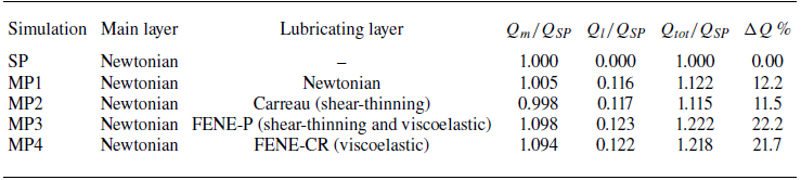


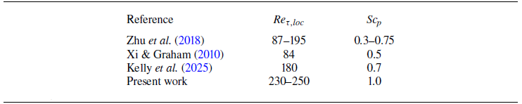


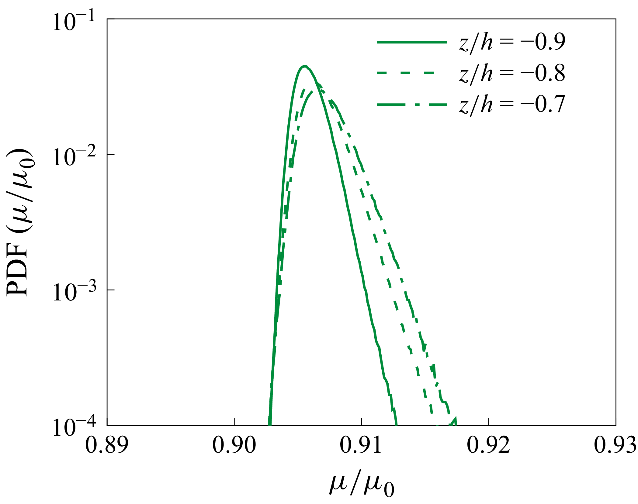


 Open access