Introduction
Obtaining large-scale direct observations at the base of an ice sheet is inherently difficult. Conversely, surface velocity observations are widely available from satellite and in situ measurements. This situation, where direct observations of one physical property are abundant while another physical property is inaccessible for direct observations, occurs in many geophysical settings and is commonly solved through inverse methods. Examples in the glaciological literature include solutions for perturbations in basal topography and basal lubrication (Reference GudmundssonGudmundsson, 2003; Reference Thorsteinsson, Raymond, Gudmundsson, Bindschadler, Vornberger and JoughinThorsteinsson and others, 2003), ice viscosity (Reference Rommelaere and MacAyealRommelaere and MacAyeal, 1997; Reference Arthern and GudmundssonArthern and Gudmundsson, 2010) and accumulation rates and patterns (Reference Waddington, Neumann, Koutnik, Marshall and MorseWaddington and others, 2007; Reference EisenEisen, 2008; Reference Steen-Larsen, Waddington and KoutnikSteen-Larsen and others, 2010). Here we concentrate on the reconstruction of basal stickiness through surface velocity observations, but the conclusions are widely applicable, and we begin with a general introduction of inverse methods.
An inverse problem is defined by the search for physical properties that cannot be directly observed, in a system where observations and an understanding of the physical system are given. In a forward sense these three parts are related by d = G(m) where d is a set of observations (data), m is a set of model parameters and G is the well-posed forward model describing the physics of the system (e.g. Reference Aster, Borchers and ThurburAster and others, 2005). In order to reconstruct model parameters, m, for given data, d, the forward model, G, has to be inverted. The process of solving an inverse problem is often unstable, in that a small change in observations can lead to a large change in the reconstructed parameters. Such problems are referred to as ill-posed. A key point is that it is commonly possible to stabilize the inversion by imposing additional constraints that bias the solution, a process that is generally referred to as regularization (Reference Aster, Borchers and ThurburAster and others, 2005).
One way to approach the inverse problem is by assessing the agreement between the observations, d, and the modeled data, G(m), through a misfit functional: J(m) = ||d − G(m)||2 (e.g. Eqn (7)). Then J needs to be rendered sufficiently small to find suitable model parameters, m. Here || . || denotes a chosen norm in the data space (e.g. the familiar L2 norm). Observations inherently contain some amount of error, and hence the exact minimizer of J will not correspond to the true model parameters. Moreover, for an unstable inverse problem it is not desirable to find an exact minimizer of the misfit functional, J, because fitting the observations below the level of error in the measurements will lead to disproportionately large unrealistic features in the model parameters, a phenomenon known as overfitting. Rather, an approximate minimizer should be sought subject to stabilizing criteria, via regularization.
Regularization
There are a number of forms of regularization; we describe several here to place our specific method in context. One method of imposing stabilizing constraints is to introduce a cost functional that contains a regularizing term. In Tikhonov regularization this is done by defining the cost functional

where α is a regularization parameter that determines how much weight should be given to J (e.g. Reference Aster, Borchers and ThurburAster and others, 2005, ch. 5). The second term involves a norm, ||| . |||, in parameter space and it regularizes the problem by giving preference to a particular solution with desirable properties. The L 2 norm, for example, would select a small solution. It might be more desirable to introduce other norms that measure the level of roughness, in order to select for smooth solutions (e.g. Reference TrufferTruffer, 2004). Non-trivial choices are necessary when choosing a value for α. Note that minimization of I with a free regularization parameter, a, would lead to ∂I/∂α = 0 = J (if that solution exists), which is not desirable. The only control on the size of J in Tikhonov regularization is through the choice of α.
A more natural approach is to incorporate the tolerance, T, in the cost function

This can be thought of as a minimization of |||m||| under the condition J = T2, and α is then a Lagrange multiplier, familiar from many optimization problems. The tolerance in the cost function prevents overfitting, and the value for α is part of the solution (Reference ParkerParker, 1994, ch. 3.02). The value of Tis chosen based on a priori estimates of measurement and model error.
For linear or linearized inverse problems the latter method is the method of choice and I(m,α) can be minimized through a direct solve (Reference TrufferTruffer, 2004) or through singular value decomposition (Reference De Paoli and FlowersDe Paoli and Flowers, 2009). For nonlinear inverse problems direct methods are impractical. Instead, the problem can be approached by iteratively minimizing J without an added smoothness term:

Calculating J(m) requires that the forward model be solved, and this definition of the misfit functional is equivalent to the one introduced by Reference MacAyealMacAyeal (1993) (his eqn (7)) or, eqn (18)) where the misfit is calculated by enforcing the model physics as a constraint (with Lagrange multipliers). If the forward problem, such as the one considered here, has a diffusive character, then iterative methods for minimizing J will tend to correct large-scale features first. Generally, iterative inverse methods start with an initial estimate for the model parameter and subsequently correct the initial estimate in each iteration. The simplest way to regularize these iterative inverse methods is to terminate the iterations when the misfit functional, J, reaches the predefined tolerance, T2; this stopping criterion is called the 'discrepancy principle' and was first suggested by Reference MorozovMorozov (1966). The final result of using the discrepancy principle as a stopping criterion in iterative inverse methods is a smooth perturbation of the initial estimate that produces modeled data, G(m), consistent with the error in the observations. Small-scale features are only added if they are justified by the observations. We refer to this as a 'principled' stopping criterion. The second stopping criterion addressed here, the recent-improvement threshold, is introduced below. It is not a principled stopping criterion, in the sense that it depends solely on the solution algorithm and is not informed by the amount of observational error.
A different approach to solving inverse problems treats the forward model as something that operates on probability distribution. This is known as the Bayesian approach and has been used in glaciology (e.g. by Reference RaymondRaymond, 2007). Data are represented as distributions (Gaussian in the case of random and independent errors). The Bayesian approach allows the use of a priori assumptions about the model parameter distribution. It is particularly useful if multimodal distributions are possible. In the case of Gaussian distributions, the Bayesian solution is identical to using an L2 norm in one of the above inverse methods (Reference Aster, Borchers and ThurburAster and others, 2005, ch. 11.2).
All regularization methods lead to a solution where additional information was added to the system in order to choose a preferred solution. This a priori information can be the choice of a priori distributions in Bayesian methods or the choice of norms in other methods. In this work we use iterative methods where I(m) = J(m) is reduced until a stopping criterion is reached. We will show that the a priori information in this case is the choice of initial estimate, and the choice of the iteration method, which also involves a choice of norms. Together with the stopping criterion this provides an implicit way of regularizing the problem.
Previous work
Reference MacAyealMacAyeal (1992) introduced iterative inverse methods to glaciology. He described the basal stickiness using basis functions whose resolution was restricted to four times the ice thickness and consequently regularized the inversion. The misfit functional was then minimized with the steepest descent (SD) method. In later work (Reference MacAyeal, Bindschadler and ScambosMacAyeal and others, 1995; Reference Vieli and PayneVieli and Payne, 2003; Reference Vieli, Payne and Du Zand ShepherdVieli and others, 2006) the tolerance was calculated but the misfit functional was completely minimized with a conjugate gradient method. Multiple sensitivity tests were performed, where the solution of an inversion was only accepted if the found minimum of the misfit functional was below the tolerance. This means that every accepted solution is a solution where a certain degree of overfitting occurred. The majority of past studies used a misfit functional without any regularization and a SD method, where the misfit functional was minimized until the change in its value in the past few iterations fell below a certain threshold (Reference Rommelaere and MacAyealRommelaere and MacAyeal, 1997; Reference Joughin, Fahnestock, MacAyeal, Bamber and GogineniJoughin and others, 2001, 2004, 2006; Reference Larour, Rignot, Joughin and AubryLarour and others, 2005; Reference Khazendar, Rignot and LarourKhazendar and others, 2007; Reference Sergienko, Bindschadler, Vornberger and MacAyealSergienko and others, 2008). We call this type of stopping criterion the 'recent-improvement threshold'. More recently, Reference Morlighem, Rignot, Seroussi, Larour, Ben Dhia and AubryMorlighem and others (2010) used Tikhonov regularization and the minimization was performed with a conjugate gradient method. Reference Maxwell, Truffer, Avdonin and StueferMaxwell and others (2008) introduced an accelerated Kozlov-Maz'ya iteration, where two alternating well-posed forward problems with different boundary conditions are solved. They employed a stopping criterion similar to the discrepancy principle. Reference Arthern and GudmundssonArthern and Gudmundsson (2010) viewed the problem as an 'inverse Robin problem', also solved two well-posed forward problems iteratively and used the same stopping criterion as Reference Maxwell, Truffer, Avdonin and StueferMaxwell and others (2008).
The current literature on iterative inverse methods that solve for the basal stickiness is dominated by two minimization methods: SD and the nonlinear conjugate gradient (NLCG) method. In some studies smoothness assumptions about the solution have been incorporated. However, the majority of past studies did not apply or discuss regularization. Without a smoothness term in the cost functional or a principled stopping criterion, two undesirable outcomes are possible. In the first case, the slowness of the iterative method can lead to a premature termination and therefore the solution does not exhibit the full resolution that would be possible given the errors in the observations (underfitting). This is especially relevant for the very slowly converging SD method. In the second case, the iterations are continued into a regime where overfitting occurs.
Outline
We use different combinations of iterative methods and stopping criteria on two synthetic datasets: a simple rectangular ice stream and a more realistic funnel-shaped ice stream. The three different minimization methods are the SD method, the NLCG method and the incomplete Gauss_Newton (IGN) method. The latter uses quadratic approximations of the misfit functional,which are minimized with the discrepancy principle. To our knowledge this iterative method is new to the field of inverse problems, not just to glaciology. We show that it leads to significantly faster convergence than either the SD or the conjugate gradient method. We implement these methods with two different stopping criteria: the discrepancy principle and the recentimprovement threshold.
Methods
Forward model
The forward model explored in this work is the shallow-shelf approximation (SSA), which was introduced by Reference MacAyealMacAyeal (1989) and approximates large-scale flow of a weak-bedded ice stream or a floating ice shelf. It is a vertically integrated approximation of the full-Stokes equations derived by small parameter arguments, and is given by
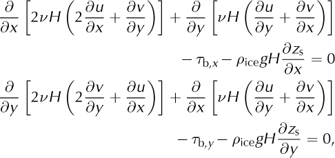
where x and y are the Cartesian coordinates defining the horizontal plane, u and v are the x and y components of velocity, ρice is the density of ice, g is the acceleration due to gravity, zs is the surface elevation, H is the ice thickness, τb,x and τb,y are the components of the basal shear stress in the x- and y-directions, and v is the effective viscosity given by
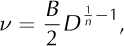
where

defines an effective strain rate, D. Here B is the depthaveraged flow rate factor and n is the flow law exponent, set to n = 3. The small term, ∊2 v, is introduced to linearize the flow law for low stresses (∊v = 1 × 10-40 s-1). We use the finite-element method and Picard iteration (i.e. computing solutions of the SSA with a viscosity determined by the previous iteration) to find numerical solutions of the forward model.
The basal shear stress is assumed to be a linear function of velocity:

where γ ≥ 0 is a scalar function of position, called the basal stickiness. One physical model for such a linear relationship is a linearly viscous till layer underneath the ice. A continuous spectrum of bed models from linear viscous to perfectly plastic is implemented in our algorithm, but only the viscous bed model is presented here. We solve for  to enforce the positivity of γ.
This model and all the algorithms below were implemented with Python, and FEniCS/DOLFIN (Reference Logg and WellsLogg and Wells, 2010) was used as the finite-element library.
The inverse problem
The inverse problem seeks to find the basal stickiness, γ (the model,m), by solving Eqns (4) given the velocity components u and v (data, d). For the purposes of this paper, all other model parameters are assumed to be well known.
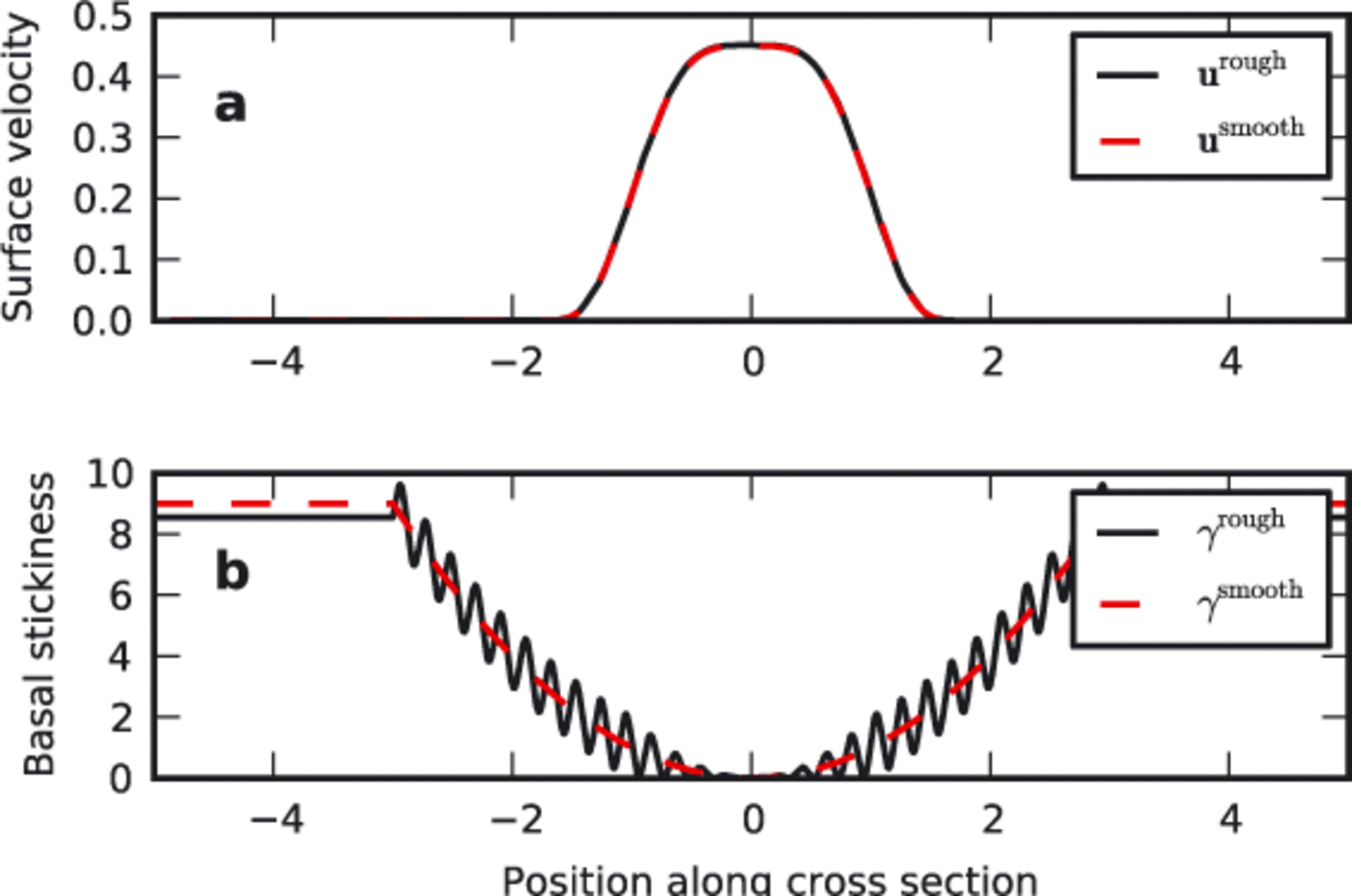
The ill-posedness of the inverse problem derives from the viscous nature of ice flow, which implies a smoothing property: high-frequency oscillations of bed stickiness are not expressed at the surface. The SSA retains this property of ice flow. For illustration, we calculate the flow through a cross section of an ice slab of uniform thickness inclined at a constant slope and with a smoothly varying basal stickiness, solved with the one-dimensional SSA (Fig. 1). This is then compared to the solution of the same problem with a high-frequency component added to the basal stickiness (black curve in Fig. 1). The two velocity responses are indistinguishable. This damping effect increases with the frequency of the oscillations, and illustrates the ill-posedness of the inverse problem:when basal stickiness is reconstructed from surface velocities, the damping becomes magnification, and the magnification is unbounded as the frequency increases.
Velocity solutions (a) to smooth (red) and highly variable (black) basal stickiness (b). The velocity solutions are indistinguishable. All plots have been non-dimensionalized.
Iterative inverse methods
The modeled surface-velocity field is calculated using the SSA given a basal stickiness function, umod(_). This model velocity field can be compared with the observed surface velocities, uobs, and we define the misfit functional

where Ω is the area of the computational domain.
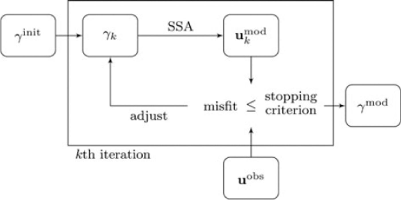
Reconstructing basal stickiness is a nonlinear inverse problem, where iterative inverse methods are most suitable. Any of the iterative methods applied in this study determine a sequence, γk, of candidate minimizers of J, starting with an initial estimate, γinit. At iteration k, a search direction, δγk, is determined, and subsequently an inexact line search is performed to find a scalar, αk > 0, such that J(γk + αk δγk) is approximately minimized. Having found the approximate minimizer in this direction, the candidate solution for the next iteration is updated,

and the algorithm is repeated (Fig. 2).
Schematic iterative inverse method, where the forward model is the SSA. For the iterative step ('adjust') we use three different iterative methods. The initial estimate of the basal stickiness is γinit, γk is the basal stickiness in the kth iteration, uk mod is the modeled surface velocity in the kth iteration and uobs are the observed data. The misfit is calculated between u™ and uobs; when the stopping criterion is met, γ mod is the final modeled basal stickiness.
Iterative methods differ in how the search directions are selected. We use three iterative methods: SD method, NLCG method and IGN method.
For well-posed minimization problems iterations continue until γk is deemed sufficiently close to the true minimizer. For an ill-posed problem this is not a good strategy: the true minimizer (if it exists) will be severely contaminated by error. The iterations must be terminated early, and we discuss two methods for doing this. One of these, the discrepancy principle, is a core ingredient of the IGN method (Eqn (21)).
Stopping criteria
All three iterative methods used tend to correct largescale features first. Intuitively this happens because largescale features are less damped in the forward problem and therefore more readily transferred to the surface. The mathematical explanation is that all three methods use the gradient of J to generate new search directions. As shown in the Appendix, this gradient is computed using an elliptic, and therefore smoothing, partial differential equation. The choice of when to stop the iteration influences the scale of features that appear in the solution. We performed experiments using the discrepancy principle, which is widely used in the inverse-problems community, as well as the recentimprovement threshold, commonly used in the glaciology community.
Discrepancy principle
The discrepancy principle stops the iterations when the desired tolerance, T, is reached:
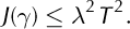
Here λ > 1 is needed for formal proofs of convergence;we used λ = 1.05 in most experiments. The tolerance is set to the expected value of all accumulated errors. If we assume a Gaussian distribution for the random uncorrelated observation errors we arrive at an expected value of
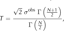
where σobs is the standard deviation of the distribution and N is the number of observations. For a derivation of this expression and a definition of the r function see Reference ParkerParker (1994, p. 123). For large N the expression above can be approximated by

The continuous version of this tolerance is where  where |Ω| is the area of the computational domain. In any case, the standard deviation, σobs, is a necessary algorithminput, here given in units of ma-1.
By stopping when the tolerance is first reached, we obtain a minimally featured correction to the initial estimate that is consistent with surface measurements. Continuing iterations beyond this point leads to the introduction of finer-scale features that are not supported by the quality of the observations, and thus leads to overfitting. In real- world applications, errors in observations are not the sole contributors to uncertainties. Model simplifications and the model parameter uncertainties that are part of the forward model also need to be included. This is addressed below in the Discussion section.
Recent-improvement threshold
Iterations are halted when the improvement in misfit functional falls below a certain threshold, Δ:

where K is a fixed delay index.
This recent-improvement threshold stopping criterion is commonly used in the glaciology community, but values for A and K are generally not reported or discussed in the literature. For the present study we used K = 10, as used by Reference Joughin, MacAyeal and TulaczykJoughin and others (2004) (personal communication from Joughin, 2010).
How this stopping criterion relates to errors in observations or models is not known, and there is no guarantee that the last iteration will not result in a significantly larger or smaller discrepancy than the tolerance expected from the data. Therefore, we do not recommend the recent-improvement threshold as a stopping criterion and are merely assessing it here because of its past use in the literature.
Choice of search directions
The three methods we used for finding a search direction all make use of the gradient of J. The definition of the gradient depends on a choice of scalar product on the space of basal stickiness functions, and we used the familiar L2 scalar product. With this choice, the gradient, ∇J(γ), is the unique function such that for any search direction, δγ,

In the case of the SSA, the computation of ∇J(γ) can be done by solving an adjoint partial differential equation that is similar to the SSA itself. Unlike most previous studies, we use the complete adjoint for the SSA (see Appendix).
Steepest descent
The most intuitive search direction is the direction of steepest descent, which leads to the rule

This method turns out to be inefficient for ill-posed problems, but these inefficiencies can sometimes be tolerable with respect to the specific problem being solved and the available computing resources.
Nonlinear conjugate gradient method
The inefficiencies of steepest descent (for linear least- squares problems) were addressed by Reference Hestenes and StiefelHestenes and Stiefel (1952) with the conjugate gradient method (see also J.R. Shewchuck, 'An introduction to the conjugate gradient method without the agonizing pain', unpublished). There, the search directions are modified from the directions of steepest descent to take into account the directions previously searched (Fig. 3). When augmented with the discrepancy principle, the linear conjugate gradient method is a standard tool for solving linear ill-posed problems (Reference HankeHanke, 1995).
Projection of a misfit functional J onto a two-dimensional (2-D) parameter space. The bold contour indicates the tolerance, T2, and every parameter combination along this contour is an equally viable solution to the inverse problem. Parameter combinations inside the tolerance are overfitting the data, and parameter combinations outside the tolerance are underfitting the data. Minimization paths of the SD (solid line) and NLCG (dashed line) methods are displayed. IGN is not easily illustrated as a 2-D projection and therefore is not shown here.

The conjugate gradient method can be generalized to nonlinear least-squares problems, although it is less well understood in this case. There is more than one generalization, and we use the Polak-Ribiere rule (Reference PressPress, 2007, p. 518) for finding search directions. We first compute a scalar,

and then a search direction,

The amount of additional coding required for the NLCG method, compared with the SD method, is negligible.
Incomplete Gauss_Newton
The Gauss_Newton method is a standard tool for minimizing nonlinear least-squares problems (Reference BjorckBjorck, 1996). Wedescribe here a modification, which we call the incomplete Gauss_Newton (IGN) method, that can be applied to solving ill-posed problems.
Let F be the map from basal stickiness, γ, to modeled velocities, umod(γ). The misfit functional can then be written as

Let F′γ denote the linearization of F at γ, so

for small variations δγ. The computation of F′γ involves solving a partial differential equation, as described in the Appendix. In the Gauss_Newton method, at iteration k we work with the linearized functional

which is a linear least-squares problem and is an approximation of the original nonlinear least-squares problem. The minimizer, δγk, of Jlin is then used as a search direction.
For an ill-posed problem, however, the linearized misfit functional, Jlin, is also ill-posed and cannot be minimized completely. Therefore, for the ‘incomplete’ Gauss_Newton method we use the linear conjugate gradient algorithm, with the discrepancy principle stopping criterion, to find regularized minimizers of Jlin. Since Jlin is only an approximation of J, there is no need to minimize it all the way to the tolerance for the full problem (T in Eqn (11)). Instead, we remove only a fraction of the remaining discrepancy. In particular, let Tk be the discrepancy of the full problem at iteration k, so

In most cases, the discrepancy for Jlin is set to
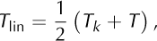
so that half the remaining discrepancy is removed when minimizing Jlin. (In practice the fraction of discrepancy to be removed is managed based on the success of the previous iteration. The IGN algorithm will be described in the mathematics literature in future papers.) The approximate minimizer, δγ, of Jlin found using the conjugate gradient method with the discrepancy principle is then used as the search direction:

Illustration of steepest descent
Descriptively, the ill-posedness of a problem can be associated with the existence of small singular values, and this ultimately leads to greatly stretched contours of the misfit functional (Reference Trefethen and BauTrefethen and Bau, 1997, lecture 4). We illustrate this by considering the projection of the misfit functional onto a two-parameter space (Fig. 3).
The tolerance, which is determined by observational errors, defines a contour along which all possible model parameter solutions lie. Figure 3 also illustrates that the selected solution of the minimization depends on the initial estimate, the tolerance and the path taken. Reduced observational errors result in a smaller tolerance, and therefore less dependence on the initial estimate. The SD (SD) method performs poorly in situations where the misfit functional is greatly stretched along some dimensions, due to the inefficient'zigzag' path. In higher-dimensional parameter spaces SD performs more poorly than indicated in Figure 3, and may not reach the tolerance at all.
Synthetic ice-stream examples
In synthetic data examples, the quality of the reconstruction can be evaluated by comparing the ‘true’ basal stickiness with the modeled basal stickiness through the following procedure:
-
1. assume a basal stickiness distribution, γtrue;
-
2. calculate the corresponding surface velocity, utrue (Eqn (4));
-
3. add Gaussian noise to simulate the random error in surface velocity observations, uobs;
-
4. use uobs in the iterative inverse method to obtain γmod.
Rectangular ice stream
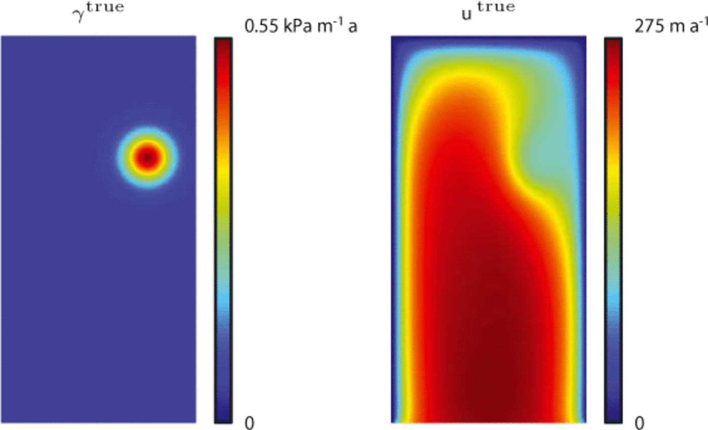
As a first simple example we define an idealized rectangular ice stream of 80 km ×160 km.We use a 60 × 120 rectangular mesh; a Gaussian bump was used for γ with the center at x0 = 60km, y0 = 110 km, a minimum value of 5 × 10⁻² kPam-1 a, a maximum value of 0.5 kPam-1a and a standard deviation of 7 × 10³m for the x- and y-directions. The flow parameter was set to B = 700 a1/3 kPa; velocity boundary conditions of zero were used on all boundaries except for the lower boundary, where a stress-free boundary was applied. The ice thickness decreases linearly from 1220m at the upstream boundary to 900m at the lower boundary. Figure 4 shows the true basal stickiness, γb true , and the resulting true surface velocity, utrue.
Map view of the magnitudes of γtrue and utrue for the rectangular ice-stream example. Dimensions: 80 km × 160 km. Mesh: 60 ×~ 120. Ice flows from top to bottom.
Funnel-shaped ice stream
To illustrate how the choice of iterative method and stopping criterion can affect the conclusions of an experiment, we recreated a synthetic ice-stream example from Reference Joughin, MacAyeal and TulaczykJoughin and others (2004). They tested sensitivity to initial estimates by considering a funnel-shaped ice stream with different sets of γ init. They did not add any random noise to the simulated surface velocities (uobs = utrue), but they re-gridded the datasets for use in the inversion, which introduced minor sampling differences. To imitate this effect, we used the synthetic ice-stream geometry and γ true with 0.45 times the gridpoints of Reference Joughin, MacAyeal and TulaczykJoughin and others (2004), then interpolated these values to the full grid and used our forward model to obtain utrue. The uobs were obtained from the forward model on the full-grid synthetic dataset. In this manner we achieved a slightly noisy set of simulated surface velocities with a mean difference between uobs and utrue of 0.8ma-1. The flow parameter was set to B = 450 a1/3 kPa.
Evaluation of results
The synthetic datasets allow a direct comparison of the final modeled basal stickiness function with the γtrue used to calculate uobs. To quantify the success of the inversion we compute the mean, μ, and standard deviation, σ, of the difference γtrue - γmod. We use μ to assess biases in the inversion and _ to evaluate the overall quality of the reconstruction. Also included is the cross-correlation coefficient, ρ, between γmod and γtrue, to evaluate how well the spatial structure is reproduced.
Results
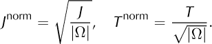
We present results from the inversion of the rectangular ice stream and the funnel-shaped ice stream with three different iterative methods: steepest descent (SD), nonlinear conjugate gradient (NLCG) and incomplete Gauss_Newton (IGN). For SD and NLCG two different stopping criteria were used (the discrepancy principle and the recent-improvement threshold). For IGN only the discrepancy principle was used as a stopping criterion, because the discrepancy principle is necessary for finding regularized minimizers of the linearized misfit functional (Eqn (21)). All examples with the rectangular ice stream use a constant basal stickiness as the initial estimate. All givenmisfit and tolerance values are normalized by the domain area and have units of ma-1:
Convergence rates
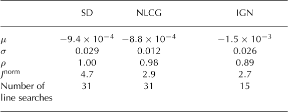
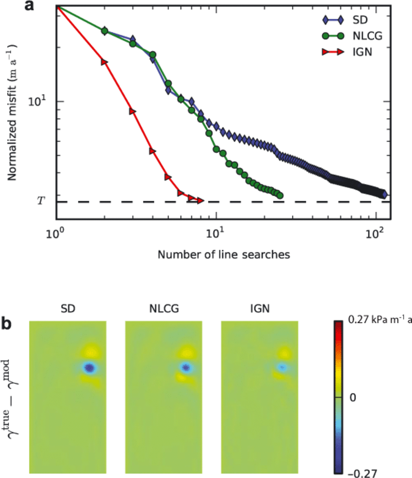
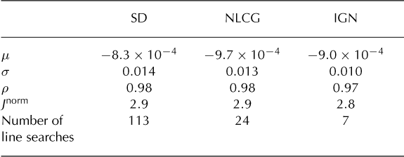
Each iteration includes a line search, and each line search involves at least one, and sometimes several, forward-model calculations. Figure 5a shows the relative performance of SD, NLCG and IGN in solving a particular inverse problem. For each iterative method, the outermost iteration is dominated by the line search where nonlinear problems are solved, so this is a good proxy for speed. IGN is consistently faster than NLCG and SD, but the ratio of the convergence rates depends on the problem set-up and the grid spacing. The reconstructed basal stickiness when using the discrepancy principle stopping criterion is virtually independent of the method of finding a search direction (Table 1). A constant initial estimate of basal stickiness and a 1% error in the simulated surface velocities were used.
(a) Convergence rates with the discrepancy principle and the rectangular ice stream for the three iterative methods. Each marker depicts a completed line search and the dashed line shows the normalized tolerance, Tnorm. The algorithm stops when λnorm is reached. (b) Map view of γtrue - γmod for the three methods (see Fig. 4 for utrue and γtrue). Areas where the inversion solution matches the ‘true’ basal stickiness well are colored green.
Evaluation of results using the discrepancy principle (Tnor m = 2.8ma-1) with three different iterative methods. The mean, μ and standard deviation, σ, of γtrue — 7mod are given in kPam-1 a. The correlation coefficient between γtrue and γmod is denoted by ρ. The misfit values, J norm, are normalized by the domain area (Eqn (23)) and have units of ma-1
Stopping criteria
Using the discrepancy principle for all three iterative methods yields minimal differences in basal stickiness solutions (Fig. 5b). Green colors in the difference plots show areas where the inversion solution matches the 'true' basal stickiness well. Even though the figure might suggest that the IGN solution issuperiorto the other two solutions, inspection of the statistics in Table 1 shows that the IGN solution obtains a marginally better fit at the expense of a slightly worse correlation coefficient.
The recent-improvement threshold stopping criterion was directly implemented in SD and NLCG, and the results for an arbitrarily chosen threshold value, of Δ = 1 ma-1, are shown in Figure 6. The solution for SD does not reach the full possible resolution, whereas NLCG coincidentally stops at the same normalized misfit value as in Figure 5.
(a) Convergence rate for SD and NLCG with the recentimprovement threshold (Δ = 1ma-1). For comparison the IGN method was continued past the discrepancy principle tolerance by setting Tnorm = 0.92 T0 norm . T0 norm is shown as a dashed line for reference. (b) Differences between the true and the modeled basal stickiness for SD, NLCG and IGN. Table 2 evaluates these results. There was a constant initial estimate of basal stickiness and a 1% error in the simulated surface velocities.

The IGN algorithm is intrinsically joined to the idea of a discrepancy principle. Therefore, the recent-improvement threshold stopping criterion could not be implemented in the algorithm. But when iterations are continued past the actual tolerance, T0 norm (by setting Tnorm = 0.92 T0 norm), a clear slowdown of the convergence can be observed and the resulting basal stickiness is overfitted (Fig. 6). The lower correlation coefficient (p = 0.89) reflects the small-scale features that are not present in the 'true' solution (Table 2).

Fitting to known error
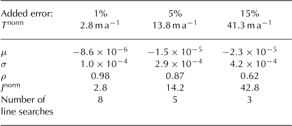
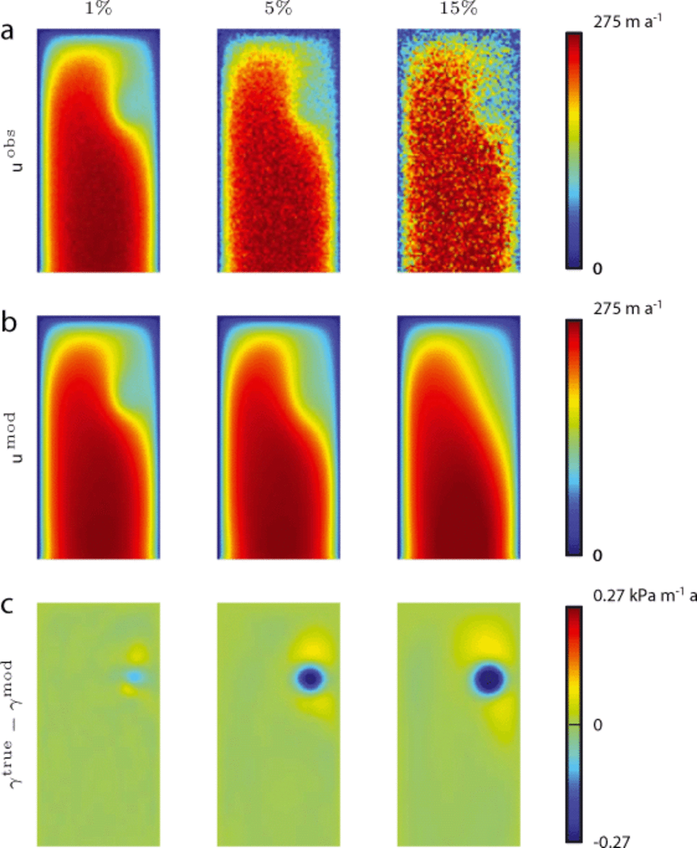
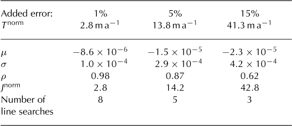
To assess the influence of error on the basal stickiness reconstruction, we performed inversions on the rectangular ice stream where the standard deviation of the added Gaussian noise is 1%, 5% and 15% of the maximum value of utrue. The standard deviation of the added random error determines the value of the tolerance used (Eqn (11)). Increased error in the simulated surface velocities leads to less capability of the model to resolve the irregularity in the velocity due to the Gaussian bump in basal stickiness (Fig. 7; Table 3).
Fig. 7. Symptoms of error in the simulated surface velocities on the resolving power of the inversion. Map view of the rectangular ice stream that flows from top to bottom. We used the IGN method and a constant initial estimate of basal stickiness. Each column shows (a) the observed velocities, (b) the modeled velocities and (c) the differences between the true and the modeled basal stickiness for that particular run. The standard deviation of the added Gaussian noise is 1%, 5% and 15% of the maximum value of utrue.
Symptoms of overfitting
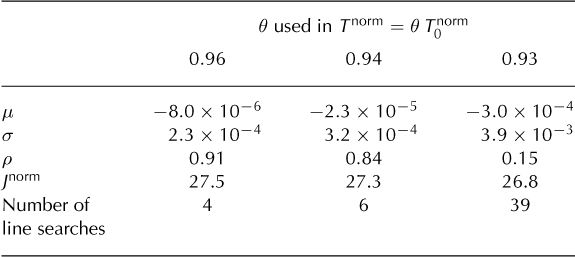
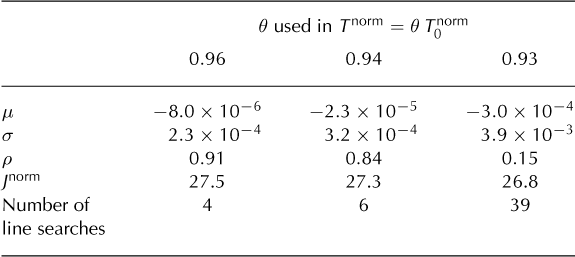
To demonstrate how the data may be overfit we performed a series of experiments where the discrepancy principle was used as a stopping criterion. Instead of using the actual normalized tolerance, T0 norm, we only used a fraction, θ, of the tolerance. This leads to a tolerance, Tnorm = θ T0 norm, where 0 ≤ θ ≤ 1. Therefore the iterations continue until that fraction of the error is matched in the modeled velocities; the values used are θ = 0.96, 0.94 and 0.93.
In the last column of Figure 8 the error in the simulated surface velocities is clearly visible in the modeled velocity, and the resulting basal stickiness contains very unrealistic features. Table 4 evaluates the results.
Symptoms of overfitting the data. Map view of the rectangular ice stream that flows from top to bottom. We used the IGN method and a constant initial estimate of basal stickiness. Each column shows (a) the observed velocities, (b) the modeled velocities and (c) the differences between the true and modeled basal stickiness for that particular run. Values of θ = 0.96, 0.94 and 0.93 were used when setting the normalized tolerance, T norm = θ T0 norm. All three runs have 10% error in the simulated surface velocities.

Dependence on initial estimates
We examined the sensitivity to different initial estimates by repeating synthetic inversions, following Reference Joughin, MacAyeal and TulaczykJoughin and others (2004). Four different initial estimates are used: γtrue ('truth'), γtrue with added noise that has a minimum wavelength of 10km ('noisy'), γ corresponding to 50% of the driving stress ('1/2 driving') and a constant γ ('constant'), as shown in Figure 9a. To recreate the previous results, we inverted for the basal stickiness with the SD method and a recent- improvement threshold of 10m a-1 over ten iterations. This arbitrary value for the threshold gave results that resembled the original work by Reference Joughin, MacAyeal and TulaczykJoughin and others (2004).
Synthetic ice-stream example reproduced from Reference Joughin, MacAyeal and TulaczykJoughin and others (2004). Ice flows from top to bottom. (a) Different initial estimates of basal shear stress: 'truth', with added noise ('noisy'), 50% of the driving stress ('1/2 driving') and a constant τb ('constant'). (b) Difference between true and modeled basal shear stress for SD method with a recent-improvement threshold of 10 ma-1 in the past ten iterations. (c) Difference between true and modeled basal shear stress for IGN method with a normalized tolerance of T norm = 1 ma-1 with λ = 1.1.
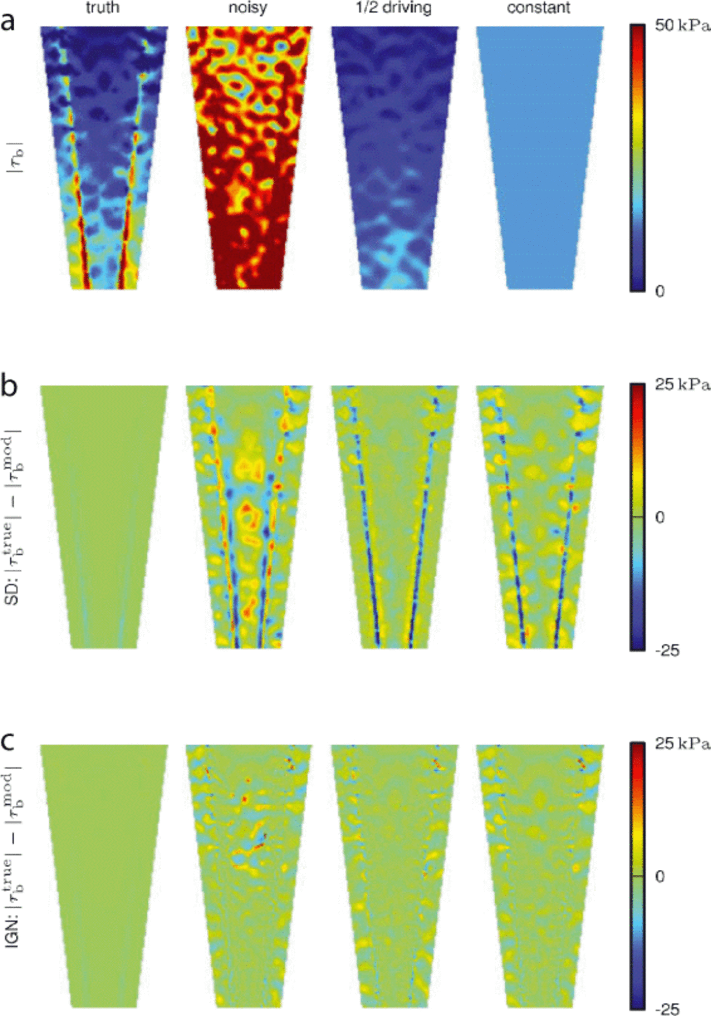
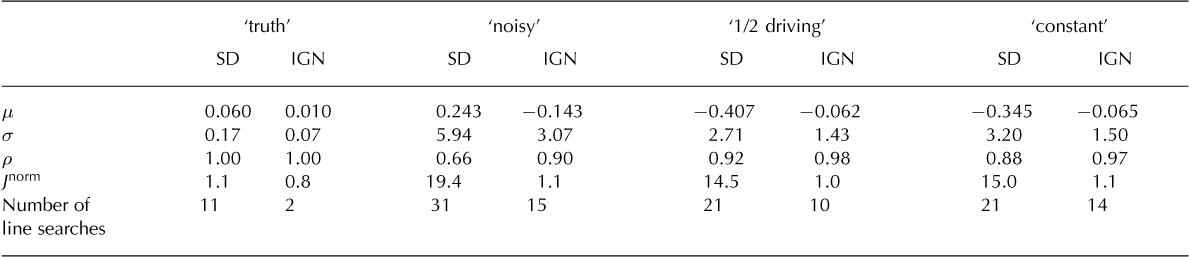
Figure 9b shows the resulting basal shear stress difference for the SD run that is comparable to figure 3 of Reference Joughin, MacAyeal and TulaczykJoughin and others (2004). Reference Joughin, MacAyeal and TulaczykJoughin and others (2004) report a value of p = 0.99 for the 'truth' example, but their figure shows discrepancies between the resulting basal shear stress and the 'true' value along the edges of the ice stream, which is also reflected in the high reported normalized misfit value of j norm = 3ma-1. Our SD 'truth' run exhibits better correspondence between the modeled and true basal shear stress: ρ = 1 and J norm = 1.1ma-1 (Table 5). These improved results are possibly due to the sampling differences mentioned in the Methods section and to our use of the complete adjoint for the SSA equations.
Table 5. Evaluation of results using four different initial estimates of basal shear stress and two different iterative methods: recent-improvement threshold (Δ = 10 m a-1) for SD and discrepancy principle (Tnorm = 1 m a-1 with λ = 1.1) for IGN (Fig. 9). (Variable description and units as in Table 1.) The variables μ, σ and ρ are calculated only over the fast-moving parts of the ice stream (area moving faster than 300 m a-1), whereas j norm covers the entire domain
We also used the IGN method with the discrepancy principle (Tnorm = 1 ma-1 with λ = 1.1) as a stopping criterion on the same synthetic dataset as above. This leads to the basal shear stress differences depicted in Figure 9c. The tolerance value T norm = 1 ma-1 was chosen as a conservative estimate of standard deviation for the set of simulated surface velocities with a mean difference between uobs and utrue of 0.8 m a-1 (Methods section).
Discussion
Convergence rates and stopping criteria
The higher efficiency of IGN (Fig. 5) makes it suitable for use with higher-order forward models and in larger domains. However, this higher convergence rate also makes it more important to choose the tolerance in the discrepancy principle correctly, because we reach the regime of overfitting faster.
The iterative solution of an inverse problem is predicated on three choices: an initial estimate, an iterative method and a stopping criterion. The experiments in Figure 5 all use the same initial estimate and tolerance, and the three methods are all based on a variation of the SD method. It should not, therefore, be surprising to obtain near-identical solutions (Table 1). The primary difference between the methods is the rate of convergence and thus the efficiency of the algorithm.
However, with uninformed stopping criteria, such as the recent-improvement threshold, the basal stickiness solutions for the different methods can show different features for the same threshold (Fig. 6). The amount of observation error is not used by the algorithm; instead it is stopped when it slows down. This occurs at different times for the different methods, so the solutions can range from underfitting to overfitting (Table 2).
For larger and more-complex systems the SD method will need a large number of iterations to reach the tolerance in the discrepancy principle and may not be a practical method to use. A probable reason for the popularity of the SD is that its convergence rate is slow enough that it does not reach the regime of overfitting. This can be an advantage because then the choice of stopping criterion is not crucial. However, it is likely to lead to underfitted solutions.
Fitting to known error
When using the discrepancy principle as the stopping criterion the iterations stop before the model attempts to fit errors in the data. Large errors in observations lead to a large tolerance, T, which results in a smaller number of line searches (Table 3). Consequently, the algorithm only makes large-scale adjustments to the initial estimate of basal stickiness, and the resulting basal stickiness has a smooth appearance as long as the initial estimate itself was smooth (Fig. 7). The quality of the reconstruction decreases as the observation error increases (Table 3; Fig. 7); however, this decreased quality does not manifest itself in a noisier appearance of the solution. With larger error in the observations we expect lower resolution in the solution, without any over- or underfitting.
Symptoms of overfitting
Fitting observation errors in the velocities means that we are trying to generate small-scale abrupt features at the surface by modifying the basal stickiness. The damping properties of the SSA lead to a magnification of these abrupt changes in the basal stickiness. This overfitting can be seen in the last column of Figure 8. Even though the SSA has the tendency to dampen and smooth jumps in basal stickiness, it is possible (at least in the simple rectangular ice stream used here) to fit a certain amount of observation error in the modeled surface velocities (Fig. 8b, last column). The positivity of the basal stickiness adds some constraint to the reconstruction but there is no other bound on the basal stickiness, so the features can get unrealistically large in order to fit the given velocities at the surface. Increased overfitting requires a sharp increase in the number of line searches necessary to produce the unrealistically large features in basal stickiness. The smoothing properties of the SSA make it difficult to fit observation errors, especially with the added constraint of positive basal stickiness. This leads to the small range of chosen θ values for the overfitting experiment (θ = 0.96, 94 and 0.93).
Dependence on initial estimates
Reference Joughin, MacAyeal and TulaczykJoughin and others (2004) found that their inversion results depended on their initial estimates, even in synthetic examples with negligible error. We suspect that this dependence on initial estimates is due to the use of the recent-improvement threshold as a stopping criterion, together with the slowly converging SD method and the resulting underfitting.
We reproduced the results shown in figure 3 of Reference Joughin, MacAyeal and TulaczykJoughin and others (2004) with the SD method and repeated the same experiment with the IGN method. Reference Joughin, MacAyeal and TulaczykJoughin and others (2004) concluded from their SD run that the '1/2 driving' initial estimate gives the best basal stickiness solution, and the same conclusion can be drawn from our SD results (Table 5). However, our IGN experiment (Fig. 9c) shows a negligible difference between the solutions for'constant' and '1/2 driving' initial estimates, and there is no dependence on initial estimates for these two cases when using IGN with the discrepancy principle. This shows the importance of achieving the maximum possible resolution. Only the 'noisy' initial estimate results in a slightly worse reconstruction when using IGN. The small-scale features that are present in the initial estimate are not corrected, which suggests that the initial estimate should not contain unjustified small-scale features. Using the SD method in this example, we were not able to obtain the resolution achieved by the IGN algorithm, even after allowing it to run for 1000 iterations.
Smoothness of a reconstruction should not be interpreted as a physical property of the basal stickiness, however, but rather as a lack of information about the solution; any additional features in the solution should be justified by the data. If in a certain situation it is known that the basal stickiness changes abruptly at a point in space, this additional information should be incorporated into the initial estimate. If the abrupt change is consistent with the observations at the surface, it will be preserved through the iterations to the final solution; if it is not consistent it will be corrected.
Modeling error
All examples in this work are synthetic examples, where the error is well known and the tolerance is well defined. Real-world situations are more complex, because in addition to observational error, there are errors introduced by the simplifications of the physical model (modeling errors), including the prescribed parameters therein. The accuracy of the prescribed parameters can sometimes be estimated, but other modeling errors are harder to quantify. In future work, synthetic experiments comparing solutions of an inverse problem using a full-Stokes model to solutions using a simplified model, such as the SSA, could give a bound on modeling errors. Additionally, the SSA is a low-order approximation of the Stokes equations, and residual terms can be calculated that give an upper bound for the modeling error. In many cases, modeling errors will quite possibly be larger than observational errors, especially when forward model parameters, such as the ice thickness, are assumed to be error-free. Reference Gudmundsson and RaymondGudmundsson and Raymond (2008) note that basal stickiness is highly sensitive to un-modeled errors in basal topography, which highlights the importance of incorporating modeling errors by adjusting the stopping criterion in iterative inverse methods or by inverting for more parameters. In the case of Gaussian assumptions for model and observation errors, modeling and observational errors simply combine by addition of the respective covariance matrices, even when the forward problem is nonlinear (Reference TarantolaTarantola, 2005, p. 35, example 1.36).
The abrupt change in slope of the IGN misfit curve in Figure 6 indicates the possible validity of the often-used 'L- curve criterion' (Reference Aster, Borchers and ThurburAster and others, 2005, p. 91). This refers to a procedure in which the tolerance is chosen at the point of the 'corner' in the misfit curve, defined by the point of maximum curvature. It defines a point at which further improvements to the misfit functional come at great cost to the norm of the solution. The sharpness of the corner will vary from problem to problem and it is not guaranteed that a clear corner will even be present. In real-world examples, where the modeling error is difficult to quantify, a rapidly converging method might give a clear point of slowdown that can serve as an estimate of the combined error in model and observations. While our results indicate that such an approach would be valid in our case, it needs to be stressed that the 'L-curve criterion' has no physical justification and has proven to be non-convergent, in the sense that the selected regularization parameter vanishes too rapidly as the noise-to-signal ratio in the data goes to zero (Reference HankeHanke, 1996).
Conclusions
Iterative inverse methods paired with a principled stopping criterion can be used to regularize and solve inverse problems. By stopping when a tolerance is reached, we obtain a minimally featured correction to an initial estimate that is consistent with observed velocities. Every ill-posed inverse problem needs to be regularized and every method of regularization requires additional information, in order to stably find a unique solution. The preferred approach presented here is the discrepancy principle stopping criterion together with the incomplete Gauss-Newton method, which is intrinsically tied to the discrepancy principle. The main advantage is that additional information needed to regularize the problem is very natural: all that is required is an initial estimate of the basal stickiness and a desired level of misfit, expressed as a normalized tolerance in ma-1.
Errors in velocity observations influence the basal stickiness solution. A stopping criterion that is informed about the amount of observation error will result in decreased resolution with increased observation error. Because the allowed misfit between observed and modeled velocity is larger with greater observation error, the algorithm will stop after correcting large-scale features. Increased noise or measurement error leads to a less-detailed solution, rather than a solution polluted with unphysical details.
Small-scale features in basal stickiness might and most likely do exist, but introducing small-scale features through overfitting must be avoided. Any features in basal stickiness should be justified by surface observations; consequently, any features in the initial estimate need to be based on prior information about the basal stickiness. If no prior information exists, a constant initial estimate is the recommended choice. For solutions of inverse problems, smoothness should be interpreted as a lack of information in the system to determine smaller-scale features.
Inevitable observation and model errors result in a risk of overfitting. Errors in observations can be largely magnified in the basal stickiness, and especially with faster-converging methods, such as incomplete Gauss-Newton this regime of overfitting can be reached easily. Consequently, the choice of a principled stopping criterion becomes even more important. TheSD method, however, has a slow convergence rate. Therefore, using SD prevents overfitting; however, it also inhibits us from reaching full resolution in the basal stickiness, and increases the dependence on initial estimates.
The benefits we observed using IGN may be of benefit to other nonlinear ill-posed inverse problems. An open- source implementation of the IGN algorithm is available as a part of 'siple: a small inverse problems library', which can be downloaded along with its tutorial from https://github.com/damaxwell/siple.
These conclusions are valid for any situation where errors are present in observations or in the model (which is always the case in real-world situations), even if only numerical errors are present. In all these situations there will be a possibility of over- or underfitting the data.
Acknowledgements
This work was supported by the US National Science Foundation (NSF CMG 0732602) and NASA MAP grant NNX09AJ38G. Ian Joughin provided data for the funnelshaped ice stream tests. Ed Bueler, Constantine Khroulev, Andy Aschwanden and Ronni Grapenthin have patiently answered questions and provided feedback. Ralf Greve acted as Scientific Editor, and Michelle Koutnik and Olga Sergienko provided detailed comments that greatly improved the readability of the manuscript.
Appendix: The Linearized Ssa, its Adjoint and the Gradient Of j
The gradient computation needed for minimizing the misfit functional, J, is usually described in the glaciology literature using the framework of constrained functional minimization and Lagrange multipliers. We give an alternative derivation that allows us to also describe the PDE computations used by the incomplete Gauss-Newton method.
To write the SSA more compactly we introduce some notation. For a velocity field u = (u1, u2), the symmetric part of the derivative of u is D(u), so
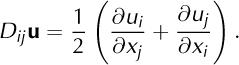
Then div u = tr Du = ∂i j ; the summation convention applies wherever an index is repeated. Given two square matrices, A = [Aij] and B = [Bij ], we define
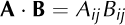
and |A|2 = A . A. The viscosity appearing in the SSA can then be written as

Assuming a linear basal stress, τb = -γu = -γ(u, v), and a driving stress, f = -ρicegH∇ zs, the SSA becomes

where ∂ ij = 1 if i = j and is zero otherwise.
Let SSA(u) denote the left-hand side of Eqn (A4). The linearized SSA (at u) is given by

So, if t is small,

A computation starting from Eqn (A5) shows that


If the SSA is being solved with periodic or Dirichlet boundary conditions, then Lu is solved with corresponding periodic or zero Dirichlet boundary conditions. The term involving ζ(u, w) has typically been omitted in previous studies with the SSA, but it is straightforward to include when it is written as above and when using the finite-element method for the numerical computations. Reference Goldberg and SergienkoGoldberg and Sergienko (2011) include the term ζ(u, w) for a hybrid ice flow model and in some cases observed improved convergence rates for steepest descent inversion using the complete versus the incomplete adjoint.
Let F(γ) be the map from basal stickiness to the corresponding solution, u, of the SSA, Eqn (A4). Implicitly differentiating Eqn (A4) with respect to u and 7 it follows that the derivative of F at γ in the direction δζ (i.e. F′ γ (δγ)) is the vector field, w, solving
Let F(γ) be the map from basal stickiness to the corresponding solution, u, of the SSA, Eqn (A4). Implicitly differentiating Eqn (A4) with respect to u and 7 it follows that the derivative of F at γ in the direction δζ (i.e. F′ γ (δγ)) is the vector field, w, solving

where (Fγ The map, Fγ , described here is used crucially in the incomplete Gauss_Newton method.
All the algorithms we use employ the L2 gradient of the misfit functional

Recall that the L2 gradient, ∇J(γ), is the unique function such that for any variation δγ,

The derivative of J at γ in the direction δγ is

where (F′γ)* is the adjoint of F′γ . So

To compute the gradient, we therefore need the adjoint of F′γ From Eqn (A7),

Just as for the matrix equation, (A-1B)* = B*(A-1)*, it follows that

for any velocity field, r. But Lu is a self-adjoint PDE, so

In summary, to compute ∇J for a given γ,
-
1. compute u = F(γ) (i.e. solve the SSA with basal stickiness γ), and
-
2. find the vector field, z, solving the linear equation, Luz = uobs - u.
Then ∇J(γ) is the scalar field, -u . z, where u and z are computed in steps 1 and 2 above.