


1. Introduction
Wind generates surface waves and induces a turbulent shear current underneath. The oscillatory convection of surface waves undulates the turbulent shear layer. The interaction between the Lagrangian drift of the surface waves and the turbulent shear layer gives rise to Langmuir circulations (LCs) (see the reviews by Leibovich Reference Leibovich1983; Thorpe Reference Thorpe2004). For strong shear, the LCs can further distort the surface waves and the boundary layer (Craik Reference Craik1982; Phillips Reference Phillips1998). These complex flow processes of wind waves set the rate at which properties exchange between the water and the air. Laboratory and field measurements supported by theoretical and numerical results have shown that the turbulence featuring LCs is significantly different from the classical turbulent boundary layer owing to the influence of surface waves (D'Asaro Reference D'Asaro2014).
The coherent circulatory motions of LCs manifest themselves by forming visible streaks, or windrows, on the water surface roughly aligned with the wind direction and extended over the wind fetch. It is widely accepted that LCs arise as an instability of the Eulerian mean flow driven by wind stress and modulated by surface waves (Thorpe Reference Thorpe2004). The equations that govern the transverse instability beneath surface waves in the presence of weak shear were first derived by Craik & Leibovich (Reference Craik and Leibovich1976), which are known as the Craik–Leibovich (CL) equations, and generalized to allow for shear of any level by Craik (Reference Craik1982) and Phillips (Reference Phillips1998). The wavelength of the transverse instability is governed by the primary mean shear and the rectified effect of the wave field exposed as the Lagrangian drift. Accordingly, the width of the LC cells, i.e. the transverse spacing between the streaks, is determined by the mean shear imparted by the wind and the dominant surface waves.
Elongated low-speed streaks can also be observed in the turbulent boundary layer near a no-slip wall (Kline et al. Reference Kline, Reynolds, Schraub and Runstadler1967). When scaled by the viscous length, the transverse spacing between the streaks exhibits a probability distribution conforming to log-normal behaviour with a universal mean value of 100 wall units (Kline et al. Reference Kline, Reynolds, Schraub and Runstadler1967; Smith & Metzler Reference Smith and Metzler1983). It has been recognized that quasi-streamwise vortices (QSVs) within the buffer region in the turbulent wall layer form the streaks by advecting the mean velocity gradient (Blackwelder & Eckelmann Reference Blackwelder and Eckelmann1979). Streaky structures were also observed on sheared turbulence bounded by a free-slip boundary (Lee & Hunt Reference Lee and Hunt1991; Rashidi & Banerjee Reference Rashidi and Banerjee1990; Lam & Banerjee Reference Lam and Banerjee1992). This suggests that the QSVs can form in the shear layer immediately beneath the wind waves and induce elongated streaks on the wavy surface. These high-speed streaks formed by QSVs of the turbulent shear layer are geometrically similar to those formed by LCs attributed to the interaction between surface waves and shear current. However, the characteristic length scales of these two vortical structures and their corresponding surface streaky footprints are distinctive.
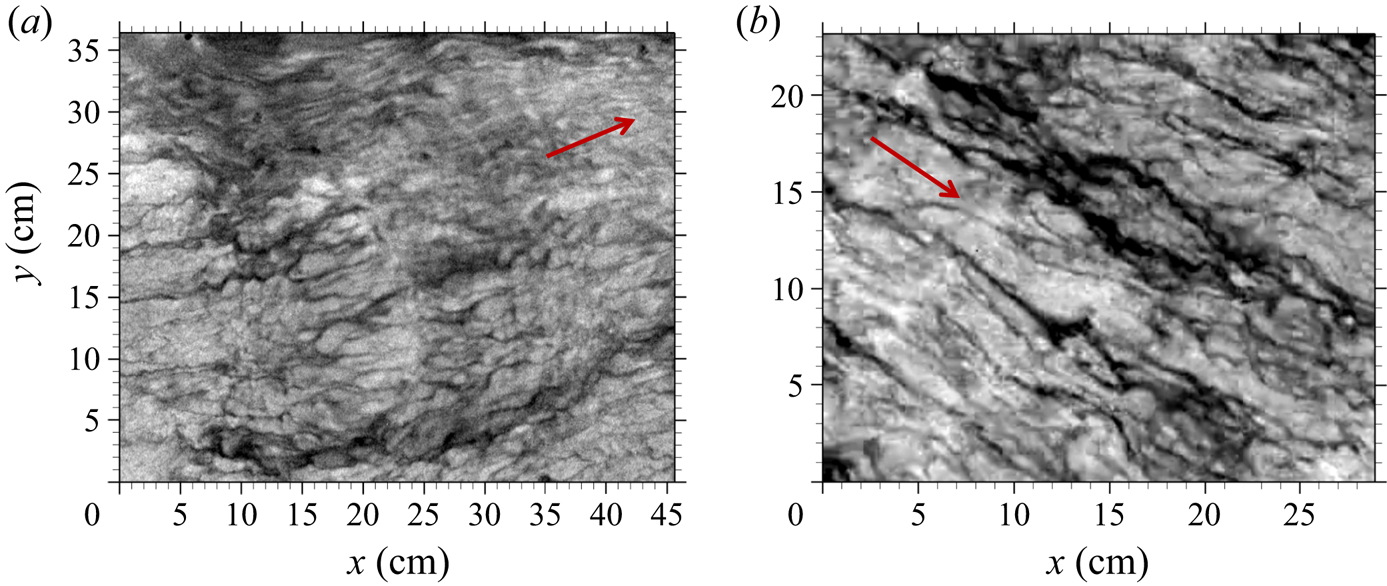
Figure 1 shows two infrared images of non-breaking wind waves taken by Schnieders (Reference Schnieders2015) (reproduced from Lu, Tsai & Jähne Reference Lu, Tsai and Jähne2019) and Smith, Handler & Scott (Reference Smith, Handler and Scott2007) (see also Handler & Smith Reference Handler and Smith2011), respectively, in two different laboratory experiments. Both infrared images exhibit wind-aligned streaky signatures of distinct length scales. In the experiments, the heat flux is upward from the water to the air, so the dark streaks in the thermal images represent cold surface water attributed to convergence flows. Predominant streaks extend in the streamwise direction over the entire image. The more intermittent and shorter streaks are observed between the predominant streaks. Such distinctness in streaky surface signatures suggests their different underlying coherent motions of varying formation mechanisms. This study aims to educe these vortical structures beneath non-breaking wind waves and the possible interaction between the vortical structures of distinct length scales.
Infrared images of wind waves taken by Schnieders (Reference Schnieders2015) (a;  $u_*=0.707\ {\rm cm}\ {\rm s}^{-1}$; reproduced from Lu et al. Reference Lu, Tsai and Jähne2019) and Smith et al. (Reference Smith, Handler and Scott2007) (b;
  $u_*=0.574\ {\rm cm}\ {\rm s}^{-1}$; see also Handler & Smith Reference Handler and Smith2011). The wind direction is indicated by red arrow. The heat flux is from the water to the air. The black-to-white grey scale represents low-to-high temperature variation. The grey scale is arbitrary and represents temperature where black is cold and white is warm.
Other experiments also revealed the correlation between the streamwise vortical structures and the surface streaks in Langmuir turbulence. Melville, Shear & Veron (Reference Melville, Shear and Veron1998) conducted laboratory experiments on the generation and evolution of streamwise vortices of various scales in a wind-driven surface shear layer. They observed that streamwise vortices are generated shortly after the first appearance of surface waves. Their experiment also demonstrated the formation and development of surface streaks accompanying that of the streamwise vortices. The subsequent laboratory experiments by Veron & Melville (Reference Veron and Melville2001) clearly show the strong influence of the streamwise vortices on the growing wave field. Both experiments of Melville et al. (Reference Melville, Shear and Veron1998) and Veron & Melville (Reference Veron and Melville2001) belong to the flow condition of a strong shear current (Craik Reference Craik1982; Phillips Reference Phillips1998). Thus Melville et al. (Reference Melville, Shear and Veron1998) and Veron & Melville (Reference Veron and Melville2001) called the vortical structures small-scale LCs.
Wave-resolved numerical simulations have also been undertaken to study Langmuir turbulence with an emphasis on validating the wave-averaged CL equations (Fujiwara, Yoshikawa & Matsumura Reference Fujiwara, Yoshikawa and Matsumura2018; Wang & Özgökmen Reference Wang and Özgökmen2018; Zhou Reference Zhou1999; Fujiwara & Yoshikawa Reference Fujiwara and Yoshikawa2020). Xuan, Deng & Shen (Reference Xuan, Deng and Shen2019) recently conducted wave-resolved large-eddy simulations (LESs) to study the underlying vortical structures and vorticity dynamics in Langmuir turbulence. They found that, in addition to the tilting effect induced by the vertical gradient of wave Lagrangian drift, the phase correlation between the vorticity fluctuations and the wave orbital straining is also important to the cumulative vorticity evolution. Such an effect is consistent with the vortex force modelling in the CL equations. The numerical study of Fujiwara et al. (Reference Fujiwara, Yoshikawa and Matsumura2018) reached a similar conclusion.
Despite the progress made by these experimental and numerical studies, to our understanding, the mutual interaction between the vortical structures of various scales in Langmuir turbulence has yet to be studied and remains intractable (Thorpe Reference Thorpe2004). Motived by the laboratory observations, the objectives of the present numerical study are twofold: firstly, to educe the underlying vortical structures of various length scales within Langmuir turbulence. Secondly, to reveal the possible interaction between these vortical structures of distinct length scales.
Note that the instantaneous flow field knows nothing of LC and QSV; instead, it achieves equilibrium by distributing energy over a spectrum of length and time scales, some more energetic than others. Langmuir turbulence is the part of that spectrum resulting from the influence of the surface waves, which act to direct energy into length scales that scale on the wavelength of the waves and form a discrete spectrum of streamwise-aligned coherent structures, which we identify as LCs. Accordingly, we identify similar structures with much shorter length and time scales as QSVs.
To proceed, we consider the most elementary situation producing Langmuir turbulence: a layer of water of infinite depth with uniform density under the action of wind of unlimited fetch with constant speed and direction. Specifically, a turbulent shear layer bounded by monochromatic surface waves and driven by stresses acting at the wavy boundary is simulated numerically. Such a model problem has previously been studied by Zhou (Reference Zhou1999), Tsai et al. (Reference Tsai, Chen, Lu and Garbe2013), Guo & Shen (Reference Guo and Shen2013, Reference Guo and Shen2014), Wang & Özgökmen (Reference Wang and Özgökmen2018), Fujiwara et al. (Reference Fujiwara, Yoshikawa and Matsumura2018), Fujiwara, Yoshikawa & Matsumura (Reference Fujiwara, Yoshikawa and Matsumura2020), Fujiwara & Yoshikawa (Reference Fujiwara and Yoshikawa2020), Lu et al. (Reference Lu, Tsai, Garbe and Jähne2021), Xuan et al. (Reference Xuan, Deng and Shen2019) and Xuan, Deng & Shen (Reference Xuan, Deng and Shen2020). In these simulations, the large-scale surface gravity waves are fully resolved. The main difference is whether the momentum dissipation process is resolved or modelled. In a direct numerical simulation (DNS), the momentum equation is solved numerically down to the viscous dissipation range without employing the subgrid-scale model (Guo & Shen Reference Guo and Shen2013; Tsai et al. Reference Tsai, Chen, Lu and Garbe2013; Guo & Shen Reference Guo and Shen2014; Fujiwara et al. Reference Fujiwara, Yoshikawa and Matsumura2018, Reference Fujiwara, Yoshikawa and Matsumura2020; Fujiwara & Yoshikawa Reference Fujiwara and Yoshikawa2020; Lu et al. Reference Lu, Tsai, Garbe and Jähne2021). Being restricted by the computation capacity, the characteristic length scale of the DNS flow is limited to less than  $O(10^2)$ cm. Therefore DNS is mainly used for mechanistic study of laboratory scale, as in the present work. In an LES, subgrid-scale modelling is used for the unresolved flow. Zhou (Reference Zhou1999) and Xuan et al. (Reference Xuan, Deng and Shen2019, Reference Xuan, Deng and Shen2020) conducted LESs of Langmuir turbulence, resolving the surface waves with wavelengths of
  $O(10^2)$ m. It is worth noting that for Langmuir turbulence of the oceanic scale, LESs employing the CL equations have been successful in replicating features attributed to LCs observed in the field, particularly in the mixed layer (e.g. Skyllingstad & Denbo Reference Skyllingstad and Denbo1995; McWilliams, Sullivan & Moeng Reference McWilliams, Sullivan and Moeng1997; Noh, Min & Raasch Reference Noh, Min and Raasch2004; Polton & Belcher Reference Polton and Belcher2007; Harcourt & D'Asaro Reference Harcourt and D'Asaro2008; Kukulka et al. Reference Kukulka, Plueddemann, Trowbridge and Sullivan2010; Deng et al. Reference Deng, Yang, Xuan and Shen2019, among many others). In comparison with the wave-resolved LES, in LES solving the CL equations, the accumulative effect of surface waves on the flow is modelled by the vortex force
  $\boldsymbol {u_s} \times (\boldsymbol {\nabla }\times \mathfrak{v})$, where
  $\boldsymbol {u_s}$ is the Stokes drift of the waves and
  $\mathfrak{v}$ is the wave-averaged rotational velocity field.
The paper is structured as follows. In § 2, the DNS employed in this study is introduced; the computational set-ups and the flow parameters of the simulation scenarios are described. Surface signatures of the simulation results are analysed using the image procession technique based on empirical mode decomposition (Lu et al. Reference Lu, Tsai and Jähne2019). The results are presented in § 3. Guided by the signatures of predominant surface streaks, a conditional average is employed to educe the vortical structures of LCs in § 4. Linear instability analysis of the wave-averaged CL equations is then conducted to determine whether the transverse width of the averaged structure is comparable to the wavelengths of the unstable transverse modes. In § 5, a detection criterion based on local analysis of the velocity-gradient tensor, and the topological geometry of the criterion are employed to extract and classify various coherent vortical structures (CVSs) associated with shear turbulence, including QSV. The spatial distributions of the QSVs and their correlation with LCs are then examined. In § 6, a method combining QSV detection and the variable-interval conditional average is developed to elucidate the preferable distributions of QSVs in the vicinity of LCs. The transport budgets of streamwise enstrophy are then examined to explain the enhanced formation of QSVs by LCs.
2. Numerical simulation of turbulent shear flow bounded by surface waves
2.1. Numerical method
We consider the three-dimensional turbulent shear flow beneath non-breaking progressive surface waves driven by surface stresses. The water density  $\rho$ and the kinematic viscosity
  $\nu$ are constants. The velocity
  $\boldsymbol {\upsilon }=(u,\upsilon,w)$ and the dynamic pressure
  $p$ of the flow field are governed by the solenoidal condition and the Navier–Stokes equations. The nonlinear boundary conditions of mass and momentum conservation, namely the conditions of material surface and continuity of tangential and normal stresses, are satisfied on the wavy surface
  $z=\eta (x,y,t)$, where
  $z=0$ is the mean surface. The advection–diffusion equation governing the evolution of the temperature field
  $\theta$ is also integrated in time with the flow simulation. The temperature is treated as a passive tracer; the buoyancy effect due to temperature fluctuations hence does not modify the vertical momentum equation.
The numerical method for solving the governing equations in a time-dependent domain subject to the fully nonlinear surface conditions was documented in Tsai & Hung (Reference Tsai and Hung2007) where details of the numerics and the implementation for simulations of various wavy flows were reported. The simulation set-up in this study is similar to that of Tsai et al. (Reference Tsai, Chen, Lu and Garbe2013). The important features of the numerical method are summarized here.
To accurately track the Lagrangian free-surface boundary and satisfy the boundary conditions, the time-dependent physical domain in  $(x,y,z)$ is mapped to a rectangular computational domain in
  $(\xi,\psi,\zeta )$ by the algebraic transformation
 \begin{equation} \xi = x, \quad \psi = y, \quad \zeta = \frac{z + h}{h + \eta(x,y,t)}, \end{equation}
where  $h$ is the constant depth, the
  $x$ and
  $y$ axes are in the streamwise and spanwise directions, respectively. The bottom and surface of the water column, therefore, are at
  $\zeta =0$ and 1, respectively. The governing equations and the boundary conditions are transformed to, and solved in, the computational domain. Such a computation strategy employing algebraic mapping has been implemented in Fulgosi et al. (Reference Fulgosi, Lakehal, Banerjee and De Angelis2003), Tsai & Hung (Reference Tsai and Hung2007), Tsai et al. (Reference Tsai, Chen, Lu and Garbe2013), Guo & Shen (Reference Guo and Shen2009), Yang & Shen (Reference Yang and Shen2011), Xuan & Shen (Reference Xuan and Shen2019) and Fujiwara et al. (Reference Fujiwara, Yoshikawa and Matsumura2020) for simulating the three-dimensional, fully nonlinear free-surface flow of viscous fluids.
The numerical model employs spectral discretization for horizontal differentials and finite differencing in the vertical with a mesh fine enough to resolve gravity–capillary waves down to capillary scale and the viscous sublayer immediately beneath the wavy surface. Low-storage Runge–Kutta scheme (e.g. Williamson Reference Williamson1980) is adopted for temporal integration of the Navier–Stokes equations for the velocity  $\boldsymbol {\upsilon }(x,y,z,t)$ and the kinematic free-surface boundary condition for the surface elevation
  $\eta (x,y,t)$. Taking the divergence of the temporally discretized Navier–Stokes equations and applying the solenoidal constraint to the velocity field at the new time interval results in a Poisson equation for the pressure. The pressure Poisson equation is solved before integrating the Navier–Stokes equations to the next time interval. The normal-stress condition is employed as the Dirichlet condition for the pressure at the free surface in solving the Poisson equation. The tangential-stress surface conditions are satisfied implicitly in integrating the horizontal momentum equations at the free surface by rearranging the conditions to evaluate the vertical derivatives of the horizontal velocities. A given uniform heat flux gives rise to a Neumann condition for the temperature field.
The validity and effectiveness of the numerical method have been demonstrated in the previous studies of wave–turbulence interaction (Tsai, Chen & Lu Reference Tsai, Chen and Lu2015; Tsai et al. Reference Tsai, Lu, Chen, Dai and Phillips2017) and the turbulent boundary layer beneath wind waves (Tsai et al. Reference Tsai, Chen, Lu and Garbe2013; Lu et al. Reference Lu, Tsai, Garbe and Jähne2021).
2.2. Simulation set-up
The simulations are initiated by superimposing an ambient fluctuation velocity field onto the velocity field of progressive, monochromatic surface waves from the nonlinear Stokes-wave solution. The surface wave is characterized by the wavelength  $\lambda$ and steepness
  $ak$, where
  $a$ is half the wave height and
  $k=2{\rm \pi} /\lambda$ is the wavenumber. The fluctuation velocity field is solenoidal and homogeneous in both the along- and cross-wind directions. Therefore, the only flow structure of the initial velocity field is the two-dimensional wavy motion in the along-wind vertical plane associated with the surface waves. The initial surface wave is imposed to shorten the spin-up time for the wave and flow fields to reach quasi-steady states (discussed in § 2.4). The simulations are carried out for at least 20 surface wave periods before the flow fields are used for analyses.
Tangential and normal surface stresses are applied at the water surface to maintain the propagation of the surface waves and the evolution of the underlying turbulent shear flow. The stress distributions are guided by the measurements of Banner & Peirson (Reference Banner and Peirson1998) and Peirson (Reference Peirson1997), and the analyses of Fedorov & Melville (Reference Fedorov and Melville1998). Despite the idealizations imposed in the numerical simulation, the computed surface elevation and surface-tangential velocity compared well with the measurements of Banner & Peirson (Reference Banner and Peirson1998) as reported in Tsai et al. (Reference Tsai, Chen, Lu and Garbe2013).
The length  $L_x$, width
  $L_y$ and depth
  $h$ of the computational domain are 4, 2 and 0.8 times the wavelength
  $\lambda$ of the surface waves and discretized by 512, 256 and 128 grids. A stretched grid system is employed such that the discretization grids cluster when approaching the surface to allow proper resolution of the viscous sublayer adjacent to the upper surface. For the simulations considered (see § 2.3), there are at least ten grids in the near-surface region
  $|z^+ |<10$, where
  $z^+=h(1-\zeta )u_*/\nu$ is the distance from the free surface in wall unit and
  $u_*$ is the mean friction velocity of water at the wavy surface.
2.3. Simulation parameters
In Lu et al. (Reference Lu, Tsai, Garbe and Jähne2021), simulations employing the above-mentioned numerical model were conducted with various initial surface-wave steepness  $ak$ and mean surface shear stress
  $\tau _0=\rho u_*^2$. These simulations are guided by a series of experiments conducted in the annular wind-wave facility Aeolotron at Heidelberg University (Schnieders et al. Reference Schnieders, Garbe, Peirson, Smith and Zappa2013; Schnieders Reference Schnieders2015). The measurement set-ups of the experiments were summarized in Lu et al. (Reference Lu, Tsai, Garbe and Jähne2021). Thermal images at various wind-wave conditions were taken in these experiments with
  $u_*$ ranging from 0.1 to
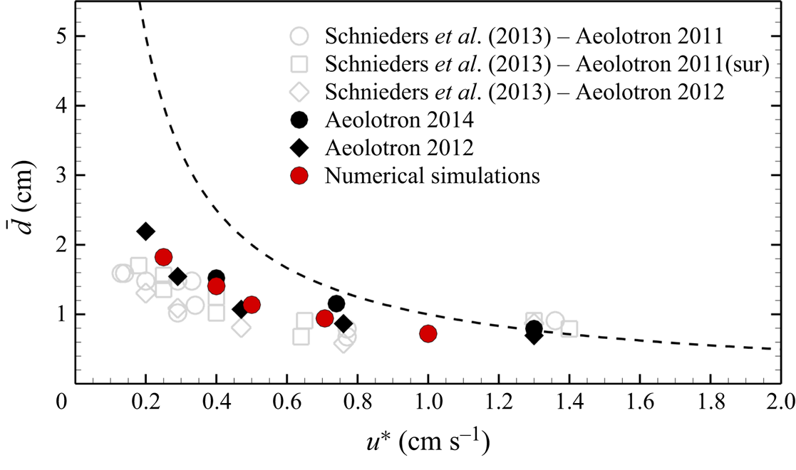
  $1.4\ {\rm cm}\ {\rm s}^{-1}$ as indicated by the black solid and open symbols in figure 2. (Figure 2 is reproduced from the results of figures 4 and 8 in Lu et al. (Reference Lu, Tsai, Garbe and Jähne2021) showing the mean surface streak spacings obtained from experiments and numerical simulations at various wind speeds. These comparisons will be further discussed in § 3.) In the experiments, non-breaking gravity–capillary waves were observed for
  $0.4\ \mbox {cm}\ \mbox {s}^{-1}\lessapprox u_*< \lessapprox 0.74\ \mbox {cm}\ \mbox {s}^{-1}$. Based on the observations, five scenarios of non-breaking wind-wave flows at
  $u_*=0.25$, 0.4, 0.5, 0.707 and
  $1\ \mbox {cm}\ \mbox {s}^{-1}$ are considered in the simulations of Lu et al. (Reference Lu, Tsai, Garbe and Jähne2021), as indicated by the solid red circles in figure 2. The simulation of
  $u_*=1\ \mbox {cm}\ \mbox {s}^{-1}$, was conducted to demonstrate the impact of non-breaking periodic waves in the high shear condition under which the surface waves observed in the wind–wave flume break. The analyses of surface thermal images by Lu et al. (Reference Lu, Tsai, Garbe and Jähne2021) further reveal that, when
  $u_* \lessapprox 0.5\ \mbox {cm}\ \mbox {s}^{-1}$, wind shear is not strong enough to maintain turbulence production.
Variations of the dimensional mean streak spacing  $\bar {d}$ with the friction velocity
  $u_*$ obtained from experiments and numerical simulations. The comparisons are reproduced from figures 4 and 8 in Lu et al. (Reference Lu, Tsai, Garbe and Jähne2021), and will be further discussed in § 3. The red solid circles denote the results obtained from the thermal surface images of the numerical simulations. The black solid symbols denote the results obtained from the infrared images taken in the experiments of Schnieders (Reference Schnieders2015) and analysed by Lu et al. (Reference Lu, Tsai, Garbe and Jähne2021). The open symbols are the results reported in Schnieders et al. (Reference Schnieders, Garbe, Peirson, Smith and Zappa2013). The dashed line depicts the scaling
  $\bar {d}u_*/\nu = \overline {d^+}=100$.
Accordingly, in the following analyses, we focus on the case of  $u_*=0.707\ \mbox {cm}\ \mbox {s}^{-1}$ in which both the non-breaking surface waves and the shear turbulence are pronounced, and their mutual interactions are significant. The final steepness of the surface waves
  $ak \cong 0.22$. The friction Reynolds number
  $Re_\tau =u_* \lambda /\nu \cong 530$, where
  $\lambda$ is the wavelength of the surface wave. The ratio of the friction velocity to wave linear phase velocity
  $u_*/c_0\cong 0.02$, which is of
  $O((ak)^2 )$. Surface waves with and without surface tension are considered to assess the impact of capillary waves. These simulations are denoted by I1 and I0, meaning intermediate-amplitude waves (denoted by I) with and without surface tension (denoted by 1 and 0, respectively). To examine the effect of carrier-wave steepness, the initial wave amplitude is reduced such that the final
  $ak \cong 0.135$. This simulation is referred to as L0, meaning low-amplitude wave (denoted by L) without surface tension. The simulation of turbulent flow bounded by a flat surface and driven by the same shear stress is also conducted for comparison with the shear turbulence beneath a wavy surface. This special case is called NW, which stands for simulation with no surface waves.
The flow parameters considered in the present simulations realize the condition in the laboratory experiments. The turbulent Langmuir numbers,  $La_t=(u_*/U_s)^{1/2}$ (McWilliams et al. Reference McWilliams, Sullivan and Moeng1997), are approximately 0.65 and 1 for cases I0 and L0, respectively, where
  $U_s=(ak)^2c_0$, corresponding to the condition of weak wave forcing considered in the typical LESs of oceanic Langmuir turbulence solving the CL equations. However, as shown in the simulation and analysis results of the following sections, the surface waves of cases I0 and L0 are strong enough to generate the large-scale vortical structures of LCs.
2.4. Decomposition and averaging of the flow field
The mobile water surface poses the difficulty of evaluating statistical properties in the fixed coordinate system of the physical domain. As such, analyses of the flow field are carried out in the wave-following coordinate defined by (2.1a–c). Since the simulated flow consists of a turbulent shear layer undulated by the oscillatory motions of the surface waves, a flow property of the instantaneous flow field,  $f(x,y,\zeta,t)$, is then decomposed into mean, wave-correlated, and fluctuation components (e.g. Sullivan, McWilliams & Moeng Reference Sullivan, McWilliams and Moeng2000; Tsai et al. Reference Tsai, Chen, Lu and Garbe2013; Xuan et al. Reference Xuan, Deng and Shen2020)
 \begin{equation} f(x,y,\zeta,t) = \bar{f}(\zeta,t) + \tilde{f}(x,\zeta,t) + f'(x,y,\zeta,t) , \end{equation}
where  $f'(x,y,\zeta,t)$ is the fluctuation component. The mean component
  $\bar {f}(\zeta,t)$ is obtained by taking the spatial average of
  $f$ over the wave-following constant
  $\zeta$ plane
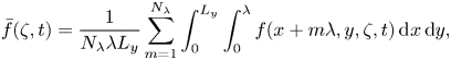 \begin{equation} \bar{f}(\zeta,t) = \frac{1}{N_{\lambda} \lambda L_y} \sum_{m=1}^{N_{\lambda}} \int_{0}^{L_y} \int_{0}^{\lambda} f(x + m\lambda, y, \zeta, t)\,{{\rm d}\kern0.06em x}\, {{\rm d}y}, \end{equation}
where  $N_{\lambda }$ is the number of surface waves in the computation domain. The wave-correlated component
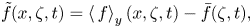 \begin{equation} \tilde{f}(x,\zeta,t)=\left\langle \,f \right\rangle_{y}(x,\zeta,t) -\bar{f}(\zeta,t), \end{equation}
where
 \begin{equation} \left\langle \,f \right\rangle_{y}(x,\zeta,t) = \frac{1}{N_{\lambda} L_y} \sum_{m=1}^{N_{\lambda}} \int_{0}^{L_y} f(x + m\lambda, y, \zeta, t) \,{\rm d}y, \end{equation}
is the phase average of  $f$. In some analyses, the ensemble average in time is also employed. They will be noted in the following discussions.
Despite the wind forcings, the wave-correlated velocities of the simulated flow field resemble closely that of a nonlinear Stokes wave, indicating the effectiveness of (2.4) in decomposing the wave-correlated components,  $\tilde {u}$ and
  $\tilde {w}$. The same finding was also reported in the wave-phase-resolved LES of Xuan et al. (Reference Xuan, Deng and Shen2019). For the simulated waves, the wave-correlated velocities decrease to 10 % of their surface values at the depth
  $z^+ \cong 200$. This depth gives a vertical length scale of the penetration depth of the LCs.
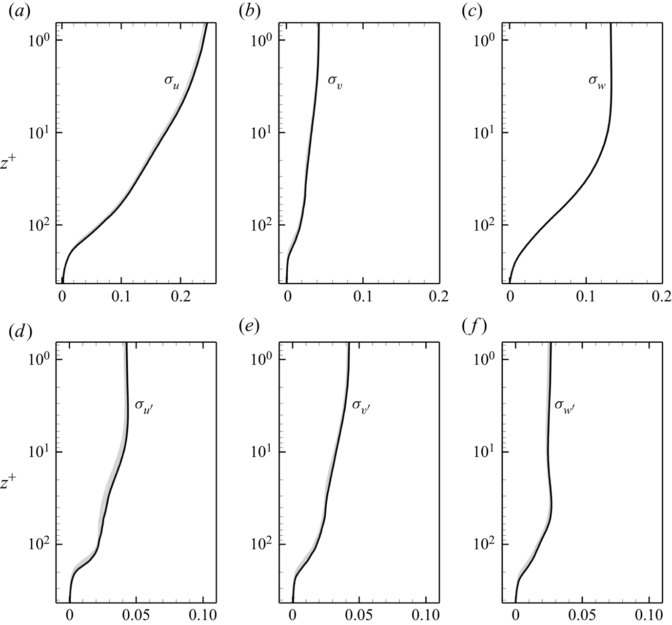
Figure 3 presents the vertical variations of the root-mean-square (r.m.s.) velocities,  $\sigma _u$,
  $\sigma _\upsilon$ and
  $\sigma _w$, and the r.m.s. fluctuation velocities,
  $\sigma _{u'}$,
  $\sigma _{\upsilon '}$ and
  $\sigma _{w'}$, of case I0 at various time instances from
  $t=25T_0$ to
  $30T_0$, where the r.m.s. of quantity
  $f$ is defined as
  $\sigma _f = (\kern0.7pt\overline {f^2})^{1/2}$. The profiles of the r.m.s. velocities exhibit strong anisotropy, with
  $\sigma _u > \sigma _w > \sigma _\upsilon$. In contrast, the fluctuation intensities,
  $\sigma _{u'}$,
  $\sigma _{\upsilon '}$ and
  $\sigma _{w'}$, are compatible with one another; this is distinct from that in turbulent wall flow, in which
  $\sigma _{u'} > \sigma _{\upsilon '} > \sigma _{w'}$. For Langmuir turbulence considered in the present simulation, the circulatory motion of LCs contributes to the decomposed spanwise and vertical fluctuation components employing decomposition (2.2), resulting in comparable fluctuation velocity partitions
  $\sigma _{u'} \sim \sigma _{\upsilon '} \sim \sigma _{w'}$. The notable fluctuating velocities, attributed to both shear turbulence and LCs, are confined within the surface layer
  $z^+ \lessapprox 200$ where the wave motions dominate the flow. The vertical distributions of these averaged fluctuation velocities change insignificantly in time, indicating the Langmuir turbulence reaches the stationary state. In the following discussions, simulated flows within this time interval are analysed.
Vertical distributions of the r.m.s. velocities,  $\sigma _u$,
  $\sigma _\upsilon$ and
  $\sigma _w$ (a–c), and the r.m.s. turbulent velocities,
  $\sigma _{u'}$,
  $\sigma _{\upsilon '}$ and
  $\sigma _{w'}$ (d–f), of case I0 at six equal-spanning time instances from
  $t=25T_0$ to
  $30T_0$. The profiles at
  $t=30T_0$ are shown in black; the rest are in grey.
3. Characteristics of surface signatures
Before proceeding to the eduction of underlying vortical structures, the characteristic surface signatures on the wavy surfaces of the simulated flows are examined following the analyses of Lu et al. (Reference Lu, Tsai, Garbe and Jähne2021). In particular, the deviation of the scaling of streak spacing on wind waves from that in wall turbulence is highlighted.
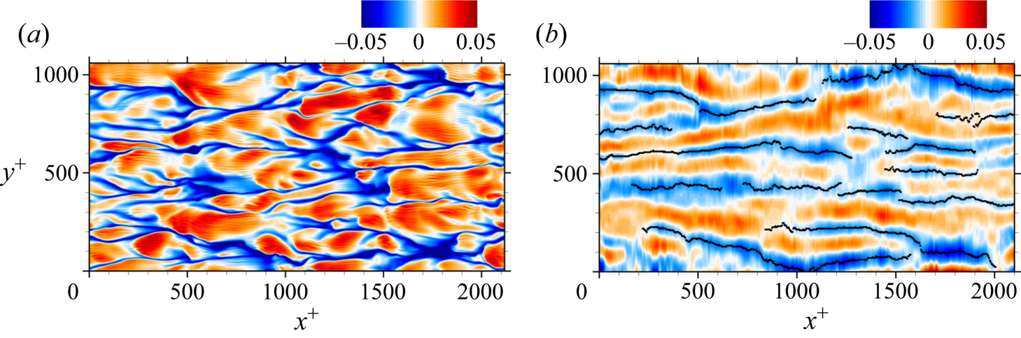
Figure 4(a) shows the temperature distributions  $\theta$ at the wavy surface from the numerical simulation of case I1. The imagery is dominated by wind-aligned elongated signatures with visible small-scale fine structures appearing among the larger-scale elongated streaks. These streaks undulate in the streamwise direction. Viewing the consecutive image sequences reveals that the undulation is associated with the cyclic streamwise compression/expansion as the surface waves propagate.
(a) Surface thermal image of case I1. Decomposed images:  $\theta _{\mathcal {W}_G}$ (b),
  $\theta _{\mathcal {W}_C}$ (c),
  $\theta _{\mathcal {V}_{LC}}$ (d) and
  $\theta _{\mathcal {V}_T}$ (e).
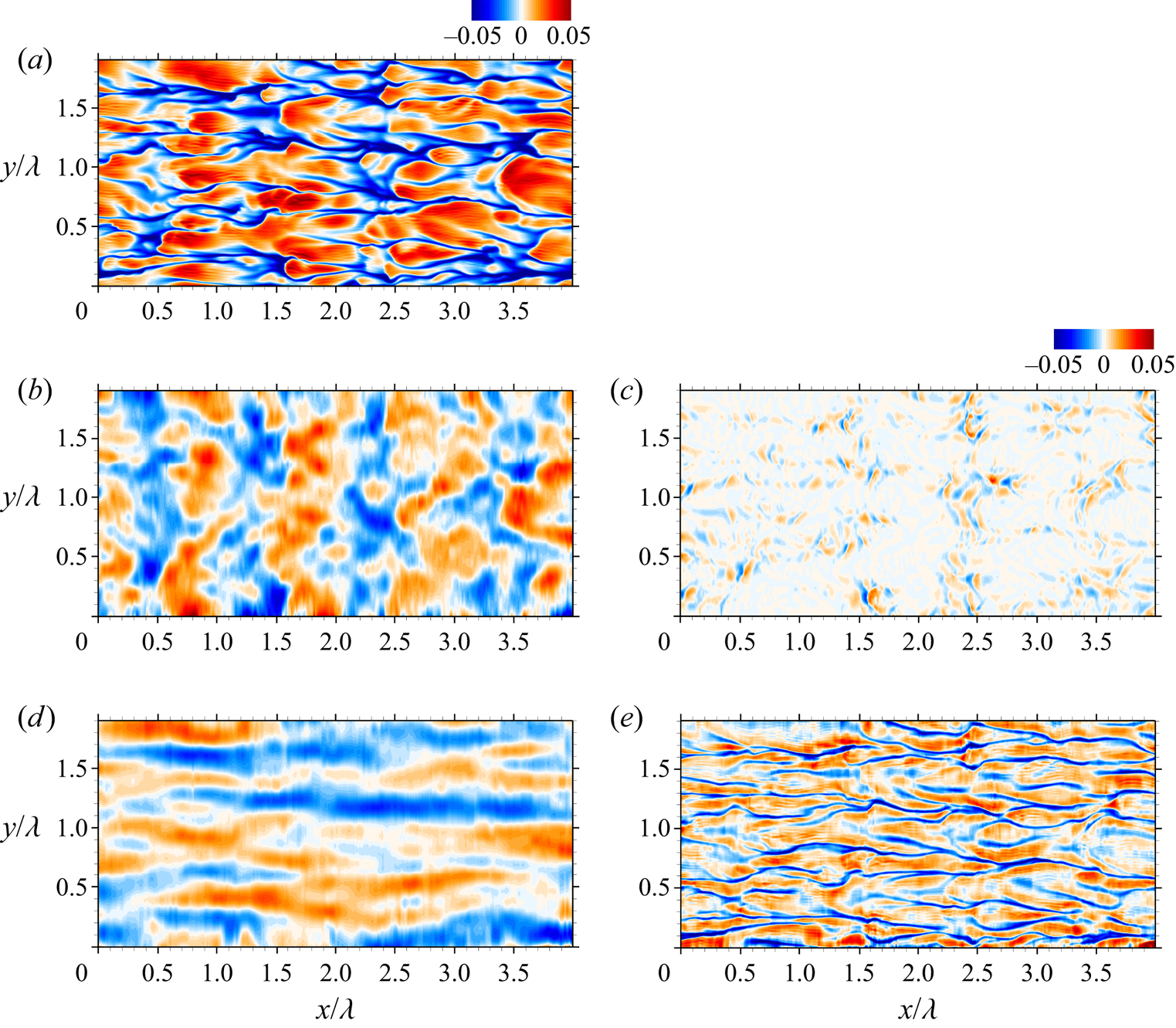
Lu et al. (Reference Lu, Tsai and Jähne2019) developed an image processing method to decompose the characteristic surface imageries induced by flow processes of different length scales and directionalities. The method utilizes the two-dimensional empirical mode decomposition algorithm of Wu, Huang & Chen (Reference Wu, Huang and Chen2009) and implements a new combination strategy based on the distinct length scales and directionalities of the signatures. This image processing method is an improvement of that in Tsai et al. (Reference Tsai, Chen, Lu and Garbe2013) which does not consider the spanwise variation of the surface waves. A brief summary of the method is given in Appendix A. Accordingly, the surface temperature distribution  $\theta$ of a wind wave is represented as
 \begin{equation} \theta (x,y) = \theta_{\mathcal{W}_G} (x,y) + \theta_{\mathcal{W}_C} (x,y) + \theta_{\mathcal{V}_{LC}} (x,y) + \theta_{\mathcal{V}_T} (x,y), \end{equation}
where  $\theta _{\mathcal {W}_G}$,
  $\theta _{\mathcal {W}_C}$,
  $\theta _{\mathcal {V}_{LC}}$ and
  $\theta _{\mathcal {V}_T}$ are the decomposed components predominantly associated with the long gravity waves, the short capillary waves, the wind-aligned streaks attributed to LCs and the quasi-streamwise streaks associated with turbulent QSVs, respectively.
The decomposed components,  $\theta _{\mathcal {W}_G}$,
  $\theta _{\mathcal {W}_C}$,
  $\theta _{\mathcal {V}_{LC}}$ and
  $\theta _{\mathcal {V}_T}$, of the simulated thermal images figure 4(a) are depicted in figures 4(b)–4(e). The results reveal distinct length scales between the decomposed gravity- and capillary-wave components,
  $\theta _{\mathcal {W}_G}$ and
  $\theta _{\mathcal {W}_C}$ (figure 4b,c), as well as the components of surface streaks attributed to LC and shear turbulence,
  $\theta _{\mathcal {V}_{LC}}$, and
  $\theta _{\mathcal {V}_T}$ (figure 4d,e). In particular, the large-scale surface streaks extend over the entire streamwise domain (four wavelengths); in contrast, the fine-scale streak footprints are shorter in streamwise length, transverse width and spacing between streaks.
The formation of the elongated streaks on the wind-sheared water surface is geometrically similar to the low-speed streaks observed in the turbulent wall layers (Kline et al. Reference Kline, Reynolds, Schraub and Runstadler1967). In the wall layers, the spacings between the low-speed streaks  $d$, when scaled by the viscous length
  $\nu /u_*$, exhibit a probability distribution conforming to log-normal behaviour with a mean value
  $\overline {d^+}=\bar {d}u_*/\nu =100 \pm 20$ for a wide range of friction velocities (e.g. Smith & Metzler Reference Smith and Metzler1983), where
  $\bar {d}$ is the mean spacing. Accordingly, further quantitative comparison between the measured and simulated results can be made by examining the transverse spacing between the elongated streaks in the decomposed image
  $\theta _{\mathcal {V}_T}$. The streak footprints in the decomposed image
  $\theta _{\mathcal {V}_T}$ can be segmented objectively using the data-driven thresholding scheme of Otsu (Reference Otsu1979). The transverse spacings
  $d$ between the segmented streaks can then be measured. Details of the procedure are reported in Lu et al. (Reference Lu, Tsai, Garbe and Jähne2021).
Figure 2 summarizes the mean spacings  $\bar {d}$ at various
  $u_*$ obtained from analysing the surface temperature distributions of numerical simulations and the infrared images of wave-flume experiments reported in Lu et al. (Reference Lu, Tsai, Garbe and Jähne2021). The results show that the mean streak spacings
  $\bar {d}$ on simulated wavy surfaces compare well with those on laboratory wind waves; albeit both are smaller than the canonical value
  $100 \nu /u_*$ for streaks next to the wall boundary. The quantitatively comparable streak spacings on the simulated wavy surfaces and laboratory wind waves suggests similar underlying flow processes inducing streaky surface signatures.
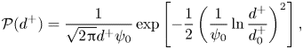
Figure 5 presents the probability density histograms of the streak spacing from analysing the simulation results of I0 ( $ak\cong 0.22$), L0 (
 $ak\cong 0.135$) and the simulated flow beneath a stress-driven flat surface (Tsai, Chen & Moeng Reference Tsai, Chen and Moeng2005; Lu et al. Reference Lu, Tsai, Garbe and Jähne2021). The mean friction velocity on the surface
  $u_*=0.707\ {\rm cm}\ {\rm s}^{-1}$ for the three simulated flows. The solid curve in figure 5 is the fitted log-normal probability density function determined from the mean spacing
  $\overline {d^+}$ and the standard deviation
  $\sigma ^+_d$ in the form
 \begin{equation}
\mathcal{P}({d}^+) =
\frac{1}{\sqrt{2{\rm \pi}}{d}^+\psi_0} \exp\left[ -\frac{1}{2} \left( \frac{1}{\psi_0}
\ln\frac{{d}^+}{{d}^+_0}\right)^2 \right],
\end{equation}
\begin{equation}
\mathcal{P}({d}^+) =
\frac{1}{\sqrt{2{\rm \pi}}{d}^+\psi_0} \exp\left[ -\frac{1}{2} \left( \frac{1}{\psi_0}
\ln\frac{{d}^+}{{d}^+_0}\right)^2 \right],
\end{equation}
where  $d^+_0=\overline {d^+}(1+\psi ^2_d)^{-1/2}$ is the median value of
  $d^+$,
  $\psi _0=[\ln (1+\psi ^2_d)]^{1/2}$ is the coefficient of variation of
  $\ln d^+$ and
  $\psi _d=\sigma ^+_d/\overline {d^+}$. For the flow bounded by a flat surface with no surface waves, the shear layer is homogeneous in the spanwise direction; the scaled streak spacing
  $d^+$ exhibits a probability distribution conforming closely to log-normal behaviour with a mean value
  $\overline {d^+} \cong 104.7$ approaching the canonical value 100 of turbulent wall layer. When surface waves are present, the scaled streak spacings deviate from the log-normal distribution and the distribution skews toward the lower value; the mean value becomes smaller than 100. Such a deviation becomes more significant as the steepness of the surface wave increases; the non-dimensional mean spacing
  $\overline {d^+}$ decreases to 85.4 in the low-amplitude waves (case L0 with
  $ak\cong 0.135$), and to 76.1 in the intermediate-amplitude waves (case I0 with
  $ak\cong 0.22$).
Probability density histograms (red vertical bars) of the cross-wind streak spacing and the fitted log-normal distributions (black lines) with the corresponding mean value for the flows of (a) case I0 with  $ak\cong 0.22$, (b) case L0 with
  $ak\cong 0.135$ and (c) flat surface without waves. The mean friction velocity on the surface
  $u_*=0.707\ {\rm cm}\ {\rm s}^{-1}$ for the three flows. The results of flow bounded by a stress-driven flat surface are reproduced from Lu et al. (Reference Lu, Tsai, Garbe and Jähne2021).
Specifically, the population of the finest streak spacings ( $\overline {d^+}\lessapprox 40$) increases considerably as the steepness of surface waves increases. This indicates that the presence of surface waves changes the distribution of underlying QSVs that induce surface streaks. One possible scenario is that the LCs, which arise from the interaction between the surface waves and the shear layer, affect the formation of QSVs and, subsequently, the distribution of surface fine-scale streaks. To validate the proposition, the characteristic vortical structures associated with the LCs and the turbulent vortices are educed by various eduction schemes in the subsequent two sections. The spatial correlation between these two vortical structures generated by different mechanisms is then examined to explore their possible interaction.
4. Large-scale structure of LCs
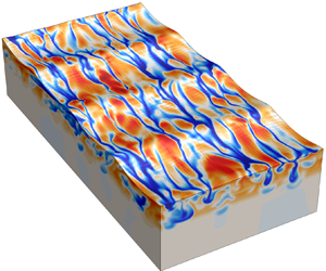
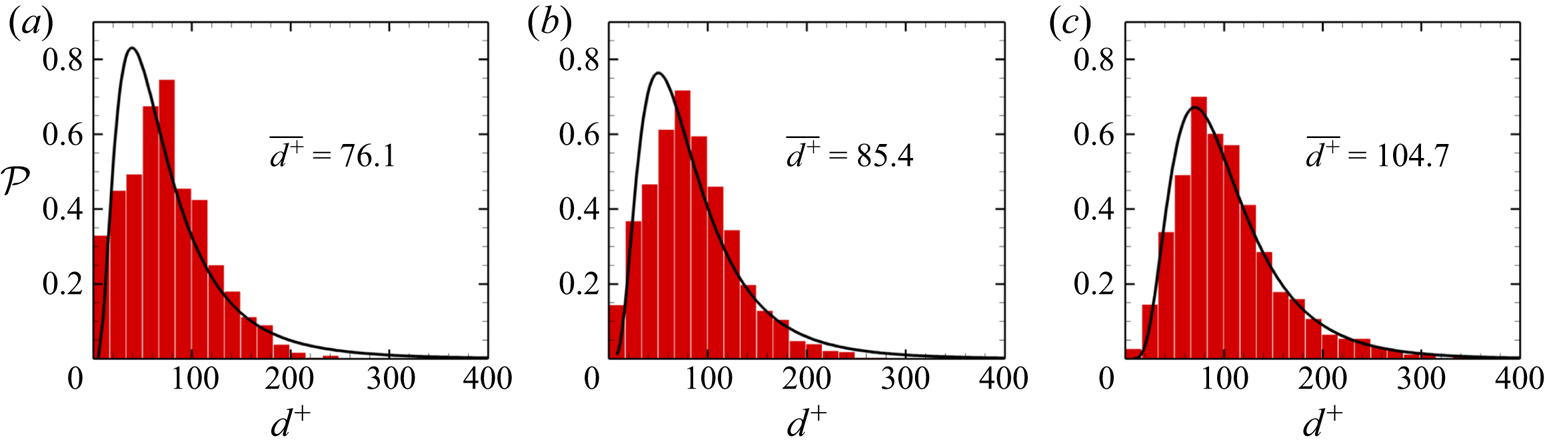
To delineate the characteristic features of the surface and flow fields, temperature distributions of cases I1 and I0 (intermediate waves with and without the surface tension, respectively) are shown in figure 6. The figure depicts the perspective view of the flow domains at  $t=30T_0$. The temperature distributions are rendered on the wavy surface, the front and side vertical boundaries. The decomposed images of large- and small-scale streaks (
 $\theta _{{\mathcal {V}}_{LC}}$ and
  $\theta _{{\mathcal {V}}_T}$) are superimposed above the wavy surface.
Perspective view of temperature distributions on the water surface, and representative along-wind and cross-wind vertical planes from the numerical simulations of cases (a) I1 and (b) I0. The waves propagate from the upper left to the lower right. The decomposed thermal images of large- and small-scale streaks are superimposed above the wavy surface. The streamwise-averaged temperature distribution is shown on the vertical plane in the lower right. The predominant cold streaks are marked by vertical arrows.
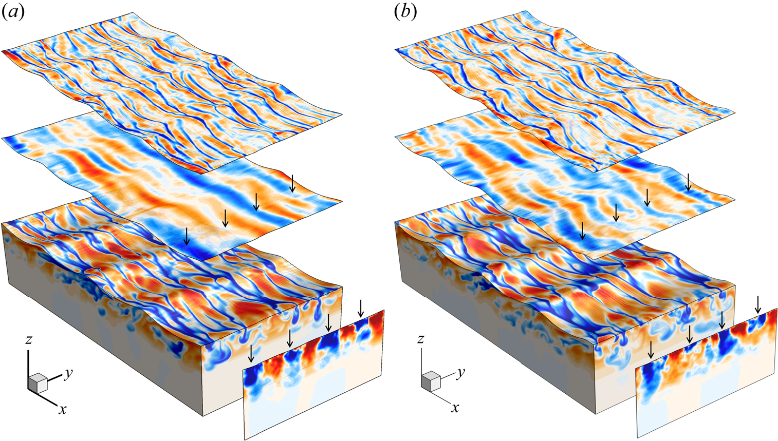
The footprints of  $\theta _{{\mathcal {V}}_{LC}}$ and
  $\theta _{{\mathcal {V}}_T}$ are characterized by the predominant and fine-scale streaks, respectively. The sub-surface flow structure associated with the predominant streaks can be elucidated by taking the streamwise average of the temperature field as shown in the vertical plane on the front. Despite meandering and bifurcation of the predominant streaks, the streamwise-averaged temperature distribution exhibits localized cold areas immediately beneath the water surface with spanwise locations roughly coinciding with the predominant surface cold streaks (marked by vertical arrows in figure 6). This supports that the predominant streaks are formed by the counter-rotating circulatory flows of the Langmuir cells. Since the streamwise length scales of the LCs are much larger than those of the QSVs of shear turbulence, taking the streamwise average of the flow field would filter out the intermittent vortices and retain only the flow structures associated with the LCs.
Comparing the temperature distributions of cases I1 and I0 shown in figure 6 reveals the insignificant difference between the simulated waves with and without surface tension. We have conducted all quantitative analyses to be present in the following sections for the flow of case I1. The results also show the minimum effect of capillary waves, consistent with the qualitative observation from figure 6. Therefore, we will focus upon the impact of gravity surface waves on the formation and distribution of vortical structures and only discuss the results of cases I0, L0 and NW in the following sections.
4.1. Conditional averaging of LCs
As shown in figure 4(d), the predominant streaks meander, and so do the axes of the large-scale vortical cells that accompany these streaks. Accordingly, streamwise averaging to educe the large-scale vortical structures can be improved by utilizing the decomposed image characterized by predominant streaks,  $\theta _{\mathcal {V}_{LC}}$. In the decomposed image
  $\theta _{\mathcal {V}_{LC}}$, the local temperature minima along various cross-wind transects are searched for as shown in figure 7(b); their horizontal coordinates are denoted by
  $(x_i,y_i)$. Connecting these coordinates forms the skeleton of the streaks. Skeletons with non-dimensional lengths less than 300 wall units are discarded. A conditional average of a physical quantity
  $q$ is then obtained by shifting the detected
  $y_i$ to the cross-wind origin of a new coordinate
  $\varUpsilon =y-y_i$ and taking the streamwise average
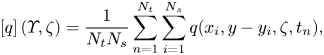 \begin{equation} \left[ q \right] (\varUpsilon, \zeta) = \frac{1}{N_t N_s} \sum_{n=1}^{N_t} \sum_{i=1}^{N_s} q(x_i, y-y_i, \zeta, t_n), \end{equation}
where  $N_s$ is the total number of detected sections, and
  $N_t$ is the total number of ensemble time instances. Here,
  $\varUpsilon = 0$ therefore becomes the symmetric plane of the counter-rotating pair of averaged LCs.
(a) Surface temperature distribution  $\theta$ of case I0 and (b) the decomposed distribution characterized by predominant streaks
  $\theta _{{\mathcal {V}}_{LC}}$. The identified skeleton of the predominant streaks is marked by black dots.
The averaged distributions of the fluctuation velocities on the cross-wind vertical plane ( $[ \upsilon ' ], [ w' ]$), and the corresponding streamwise vorticity
  $[ \omega _{x}' ]$ of the simulations I0 and L0 are shown in figure 8. The result reveals a more orderly cellular structure, consistent with the counter-rotating circulatory flow of LCs: the averaged flow converges near the surface and diverges in the submerged water, resulting in a downwelling beneath the surface streak (
 $\varUpsilon = 0$) and upwellings on both sides of the structure. The surface converging velocities are more significant than the submerged diverging velocities; the downwelling is stronger than the upwellings, and both decay rapidly with depth.
The averaged distributions of the fluctuation velocities on the cross-wind vertical plane ( $[ \upsilon ' ], [ w' ]$), and the corresponding streamwise vorticity
  $[ \omega _{x}' ]$ of cases I0 (a–c) and L0 (d–f). The ensemble averaging is taken from
  $t=25T_0$ to
  $30T_0$ for case I0 and from
  $t=30T_0$ to
  $35T_0$ for case L0.
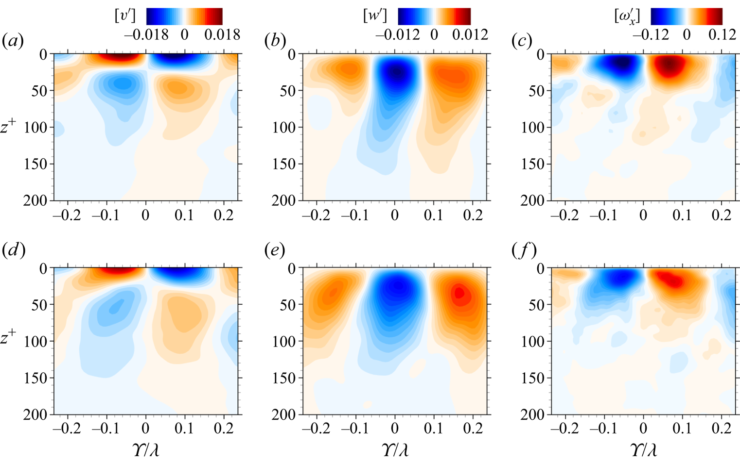
The averaged structure depicted in figure 8 also reveals the characteristic cross-wind length scale of the predominant LCs. The transverse span of a pair of Langmuir cells,  $d_s$, can be estimated as the width between the two zero spanwise velocity contours at the water surface. For both cases I0 and L0, the estimated width of an averaged LC pair
  $d_s\cong 0.34\lambda$ (see figure 8a,d), resulting in a non-dimensional wavenumber
  $\ell _s=\lambda /d_s \cong 2.9$. Despite the comparable transverse length scales, the maximum velocities and the core vorticity of the averaged LCs of I0 are stronger than those of L0; the maximum
  $[ \upsilon ' ]$ and downwelling
  $[ w' ]$ of I0 are approximately 1.3 times those of L0, the maximum
  $[ \omega _{x}' ]$ of I0 is approximately 1.5 times that of L0.
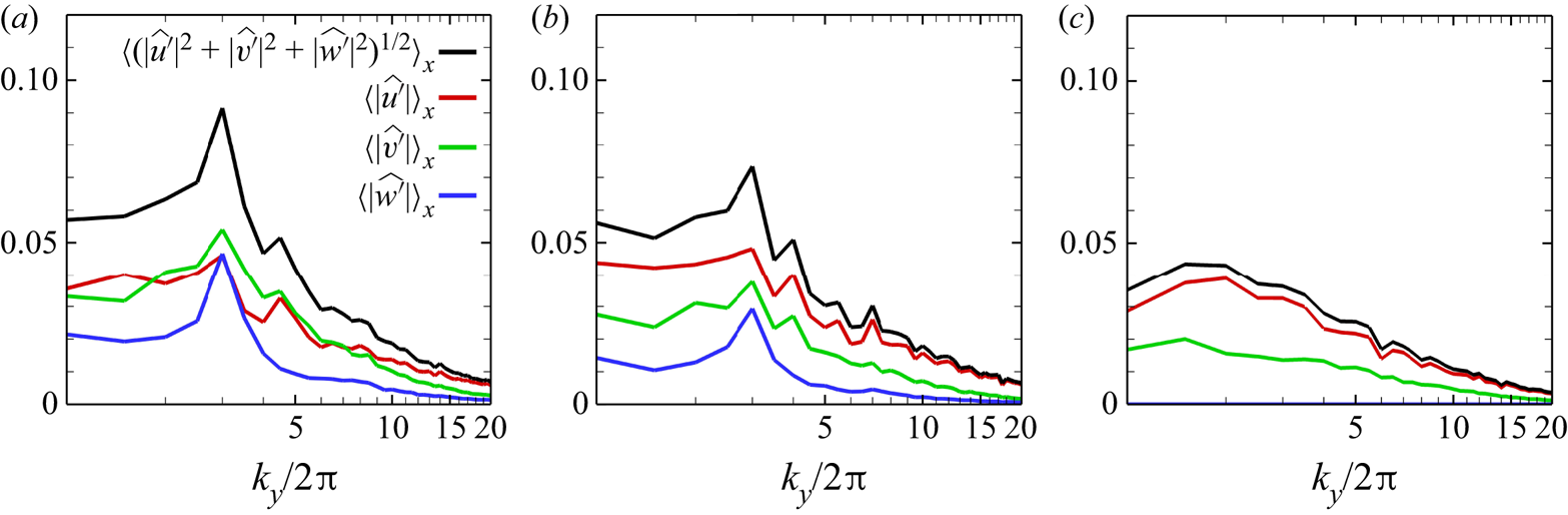
The transverse length scale of the large-scale vortical structure can also be revealed from the velocity spectrum of the flow field. Figure 9 presents the streamwise averages of the spectral density distributions of the fluctuation velocities,  $\langle {\lvert \widehat {u'}\rvert }\rangle _x$,
  $\langle {\lvert \widehat {\upsilon '} \rvert }\rangle _x$ and
  $\langle {\lvert \widehat {w'} \rvert }\rangle _x$, and the turbulent kinetic energy,
 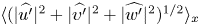 $\langle {(\lvert \widehat {u'} \rvert ^2 + \lvert \widehat {\upsilon '} \rvert ^2 + \lvert \widehat {w'} \rvert ^2)^{1/2}}\rangle _x$, at the surface, where
  $\langle {\cdot }\rangle _x$ is the streamwise average,
  $\widehat {\boldsymbol {\upsilon }'}(x,k_y)$ is the Fourier transform of
  $\boldsymbol {\upsilon }'$ and
  $k_y$ is the non-dimensional spanwise angular wavenumber. The distributions clearly show peaks at
  $k_y/2{\rm \pi} =3$ for cases I0 and L0, which is very close to the transverse wavenumber
  $\ell _s\cong 2.9$ of the averaged vortical structure depicted in figure 8. The amplitudes of the
  $\upsilon '$ and
  $w'$ spectra of case I0 are higher than those of case L0, consistent with the averaged structure. In contrast, the velocity spectra are broad-banded for case NW with no surface waves; no peak spectra of velocities are observed.
The streamwise averages of the spectral density distributions of the fluctuation velocities,  $\langle {\lvert \widehat {u'}\rvert }\rangle _x$,
  $\langle {\lvert \widehat {\upsilon '} \rvert }\rangle _x$ and
  $\langle {\lvert \widehat {w'} \rvert }\rangle _x$, and the turbulent kinetic energy,
  $\langle {(\lvert \widehat {u'} \rvert ^2 + \lvert \widehat {\upsilon '} \rvert ^2 + \lvert \widehat {w'} \rvert ^2)^{1/2}}\rangle _x$, of cases I0 (a), L0 (b) and NW (c).
4.2. Stability analysis of the CL equations
The results presented so far clearly reveal the possible formation of Langmuir cells beneath the surface waves. It is widely accepted that LC arises through the interaction of the Lagrangian drift of the surface waves with the shear current. Perturbations to the shear current result in distortion of the vortex lines initially comprising spanwise vorticity  $\bar {\omega }_y(z)$. Despite the distortion, each vortex line advects at its original velocity plus Stokes drift
  $U_s$. Since
  ${\rm d}U_s/{\rm d}z\ne 0$, the distorted vortex lines are then exposed to different values of
  $U_s$ at different
  $z$, the vortex line is tilted to realize streamwise vorticity. The equations that govern this process beneath irrotational surface waves in the presence of weak shear were first derived by Craik & Leibovich (Reference Craik and Leibovich1976), and are known as the CL equations. The CL equations are wave averaged in the sense that they exploit the fact that LC evolves over a longer time scale compared with the wave period and so take an average over the wave field. The rectified effect of the wave field is then exposed as the Stokes drift. But for the streamwise vorticity to realize the spanwise and vertical velocities and thus circulatory rolls requires an instability mechanism.
To proceed, following Leibovich & Paolucci (Reference Leibovich and Paolucci1981) and Phillips (Reference Phillips2001), we consider the linearized CL equations, which can be written as
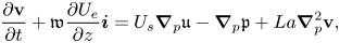 \begin{equation}
\frac{\partial \mathfrak{\textbf{v}}}{\partial t} + \mathfrak{w}
\frac{\partial U_e}{\partial z} \boldsymbol{i} = U_s \boldsymbol{\nabla}_p \mathfrak{u} - \boldsymbol{\nabla}_p
\mathfrak{p} + La \boldsymbol{\nabla}_{p}^2 \mathfrak{\textbf{v}},
\end{equation}
\begin{equation}
\frac{\partial \mathfrak{\textbf{v}}}{\partial t} + \mathfrak{w}
\frac{\partial U_e}{\partial z} \boldsymbol{i} = U_s \boldsymbol{\nabla}_p \mathfrak{u} - \boldsymbol{\nabla}_p
\mathfrak{p} + La \boldsymbol{\nabla}_{p}^2 \mathfrak{\textbf{v}},
\end{equation}
where  $\mathfrak{\textbf{v}}(y,z,t) = \mathfrak {u}\boldsymbol {i} + \mathfrak {v}\boldsymbol {j} + \mathfrak {w}\boldsymbol {k}$ is the non-dimensional wave-averaged perturbed rotational velocity,
  $U_e$ is the Eulerian mean velocity,
  $\mathfrak {p}$ is the wave-averaged perturbed pressure and
  $\boldsymbol {\nabla }_p = \partial / \partial y \boldsymbol {j} + \partial / \partial z \boldsymbol {k}$. The above process to realize the streamwise vorticity of LCs is captured in the vortex force term
  $U_s \boldsymbol {\nabla }_p \mathfrak {u}$. In the non-dimensional equation (4.2), the characteristic length scale
  $\mathcal {L}=k^{-1}$; the streamwise velocity is non-dimensionalized by the characteristic velocity scale
  $\mathcal {U} = u_*^2\nu _T^{-1} k^{-1}$, where
  $\nu _T$ is the eddy viscosity; the spanwise and vertical velocities are non-dimensionalized by
  $\mathcal {V} = \mathcal {U}^{1/2} U_s^{1/2}$; the time is non-dimensionalized by
  $\mathcal {L/V}$; and the pressure is non-dimensionalized by
  $\rho \mathcal {V}^2$. This form then exposes the Langmuir number defined as
  $La = \nu _T \mathcal {V}^{-1} \mathcal {L}^{-1}$.
In the CL equation (4.2), the basic state consists of surface waves of  $ak\sim O(\epsilon )$ and a weak Eulerian mean shear flow (Craik Reference Craik1982). The level of shear is quantified by
  $\mathcal {U}/c\sim O(\epsilon ^s)$, where
  $c$ is the phase velocity of the waves and the exponent
  $s\ge 0$ (Phillips Reference Phillips1998, Reference Phillips2001). For a weak mean shear flow,
  $s=2$, the characteristic scales of the perturbed velocities are
  $\mathcal {U}\sim O(\epsilon ^2)$ and
  $\mathcal {V}\sim O(\epsilon ^2)$. For stronger but still weak shear,
  $s=1$, the CL instability mechanism, i.e. (4.2), is essentially unchanged, apart from scaling factors (Craik Reference Craik1982); the characteristic scales of the perturbed velocities become
  $\mathcal {U}\sim O(\epsilon )$ and
  $\mathcal {V}\sim O(\epsilon ^{3/2})$.
The CL equation (4.2) admits two instability mechanisms, CL types 1 and 2 (CL1 and CL2), according to whether the wave drift  $U_s$ varies laterally. Since our simulations impose unidirectional surface waves, the averaged large-scale vortical structures observed in figure 8 are likely to be formed by the CL2 instability; and the spanwise width of the averaged LC pair would be close to the wavelength of the most unstable spanwise disturbance.
Transverse instability of the rectified flow is then sought by assuming the disturbance to be spanwise periodic with wavenumber  $\ell$ and represented by the normal mode
 \begin{equation}
\mathfrak{\textbf{v}} =
\hat{\mathfrak{\textbf{v}}}(z) {\rm Re} \left\{ {\exp}
\left( {\rm i}\ell y +\sigma t \right) \right\} \quad
\mbox{and}\quad{\mathfrak{p}} = {\hat{\mathfrak{p}}}(z)
{\rm Re} \left\{ {\exp} \left( {\rm i}\ell y +\sigma t
\right) \right\}, \end{equation}
\begin{equation}
\mathfrak{\textbf{v}} =
\hat{\mathfrak{\textbf{v}}}(z) {\rm Re} \left\{ {\exp}
\left( {\rm i}\ell y +\sigma t \right) \right\} \quad
\mbox{and}\quad{\mathfrak{p}} = {\hat{\mathfrak{p}}}(z)
{\rm Re} \left\{ {\exp} \left( {\rm i}\ell y +\sigma t
\right) \right\}, \end{equation}
where the spanwise wavenumber  $\ell$ is equivalent to the ratio of the wavelength of surface wave to the wavelength of spanwise disturbance, and
  $\sigma$ is complex. Substituting (4.3a,b) into the linearized CL equation (4.2), representing
  $\hat {\mathfrak{\textbf{v}}}$ and
  $\hat {\mathfrak {p}}$ by Chebyshev polynomials and using the collocation technique results in a generalized complex eigensystem for the truncated polynomial coefficients as the eigenvector and
  $\sigma$ as the eigenvalue. The transverse disturbance is unstable when the growth rate
  $\mbox {Re} \{ \sigma \} \equiv \sigma _r > 0$. For the analysis of asymptotic stability considering constant mean velocity shear as
  $t\rightarrow \infty$, we concur with the results of Tsai et al. (Reference Tsai, Lu, Chen, Dai and Phillips2017) employing the Galerkin technique of Phillips (Reference Phillips2001) up to two decimal places. The critical reciprocal Langmuir number
  $La_c^{-1}$ and its corresponding critical wavenumber
  $\ell _c$ computed using the Galerkin and collocation techniques are
  $(La_c^{-1},\ell _c )=(2.1435,0.3182)$ and
  $(2.1383,0.3247)$, respectively. Note that these values of
  $La_c^{-1}$ are higher than the 1.46 and 1.4395 globally stable values reported, respectively, by Leibovich & Paolucci (Reference Leibovich and Paolucci1981) and Phillips (Reference Phillips2001) because of a factor of 2 difference in the magnitude of the Stokes drift.
For stability analysis of the simulated flow, the mean shear velocity  $U_e$ is computed from the ensemble average of the mean streamwise velocity
  $\bar {u}$ when the flow reaches a stationary state. The wave drift profile
  $U_s$ is calculated by the second-order Stokes drift since the wave-correlated velocities
  $(\tilde {u},\tilde {w})$ of the simulated flow field closely resemble those of a third-order Stokes wave. The eddy viscosity
  $\nu _T$ is evaluated by taking the average of
  $-\overline {u'w'} ( {\rm d}\bar {u} / {\rm d}z )^{-1}$ over the entire computation water column. For both cases I0 and L0, the exponent of the shear index
  $s$ ranges from 0.8 to 1.3, indicating the basic state consists of a weak Eulerian mean shear flow, and the CL equation (4.2) can be used to explain the formation mechanism of observed large-scale vortical structures.
Stability diagrams of the CL equation showing the range of unstable wavenumber  $\ell$ for varying reciprocal Langmuir number
  $La^{-1}$ of cases I0 and L0 are presented in figures 10(a) and 10(c). The thick, solid lines mark the margin of the neutral stability boundary. Variation of the most unstable wavenumber
  $\ell$ with
  $La^{-1}$ is depicted by the thick, red dashed line. Contour lines of various fractions of the maximum growth rate
  $\sigma _r^{max}$ are superimposed on the instability region by the dashed lines. Also presented in figures 10(b) and 10(d) are the corresponding evolutions of the reciprocal Langmuir number
  $La^{-1}$ with time. The reciprocal Langmuir number decays rapidly from the unrealistic values of
  $O(10^{6\sim 8})$ in the early stage of the simulation to 85 at
  $t\cong 15T_0$ for case I0 and to 80 at
  $t\cong 23T_0$ for case L0. After this simulation spin-up period,
  $La^{-1}$ approaches asymptotically to
  $\sim$40 at
  $t\cong 30T_0$ for case I0 and to
  $\sim$35 at
  $t\cong 40T_0$ for case L0. Therefore, the subsequent evolution of the Langmuir turbulence can be considered as being dominated by the most unstable transverse instabilities incepted at
  $t\cong 15T_0\sim 16T_0$ with
  $La^{-1}\cong 80\sim 85$ for case I0, and at
  $t\cong 24T_0\sim 25T_0$ with
  $La^{-1}\cong 49.5\sim 52$ for case L0. From the stability diagram, the corresponding wavenumber of the unstable mode with the maximum growth rate is
  $\ell _{max}\cong 2.7\sim 2.9$ for case I0 and
  $\ell _{max}\cong 2.65\sim 2.77$ for case L0. These
  $\ell _{max}$ of the instabilities with the maximum growth rates are close to the wavenumber
  $\ell _s \cong 2.9$ of the averaged vortical structure depicted in figure 8. The close wavenumbers of the most unstable modes of cases I0 and L0 also explain that the two instabilities grow into vortical structures of similar transverse length scales shown in figure 8.
Stability diagrams of the CL equation showing the range of unstable wavenumber  $\ell$ for varying reciprocal Langmuir number
  $La^{-1}$ of cases I0 (a) and L0 (c). The thick, black solid lines mark the margin of neutral stability. Variation of the most unstable wavenumber with
  $La^{-1}$ is depicted by the thick, red dashed line; variations of unstable wavenumber with fractions of maximum growth rate are depicted by the thin, black dashed lines (
 $0.9\sigma ^{max}_r$,
  $0.7\sigma ^{max}_r$ and
  $0.5\sigma ^{max}_r$). Temporal evolutions of the reciprocal Langmuir number
  $La^{-1}$ of cases I0 (b) and L0 (d).

Note that the instability of the linearized CL equations (4.2) depends on the Eulerian mean velocity  $U_e$ and the Stokes drift of the waves
  $U_s$. These two velocity profiles are different for cases I0 and L0. However, the ranges of
  $\ell _{max}$ of the corresponding
  $La^{-1}$ are similar for the two waves of different steepnesses. Whether such similarity is due to the coincidence of the spin-up processes in the simulations is not conclusive. In contrast, the two instabilities of similar transverse length scales develop into vortical structures of different strengths for surface waves of different steepnesses. In the CL equations, the cumulative effect of the waves appears as the vortex force,
  $\boldsymbol{\mathcal {f}}_{\boldsymbol{\!v}}=\boldsymbol {u_s} \times (\boldsymbol {\nabla } \times \mathfrak{v})$, driving the counter-rotating Langmuir cells. Therefore, steeper surface waves accompanying larger wave drift
  $\boldsymbol {u_s}$ result in a stronger vortex force that intensifies the vortical structures of LC, as revealed by the averaged structures of cases I0 and L0 in figure 8.
It should also be emphasized that the less unstable modes of other wavelengths can also develop into LCs with a wide range of transverse length scales. They are filtered out in the averaging process of § 4.1.
5. Small-scale CVSs
The distinct spatial scales of the streaky signatures in the decomposed thermal images  $\theta _{{\mathcal {V}}_{LC}}$ and
  $\theta _{{\mathcal {V}}_T}$ depicted in figures 4 and 6 possibly suggest different flow processes underneath to form the elongated surface streaks. For a turbulent shear flow next to a no-slip wall, the QSVs manifest themselves in the form of elongated low-speed streaks in the immediate proximity of the wall (Kline et al. Reference Kline, Reynolds, Schraub and Runstadler1967). Likewise, similar CVSs can also arise in the wind-driven shear layer inducing high-speed surface streaks.
5.1. Eduction of CVSs
There exist various methods to identify CVSs within turbulent shear flows. In these methods, the swirling core of a CVS is defined by mathematical criteria based on the local analysis of the velocity-gradient tensor  $\boldsymbol {\nabla }\boldsymbol {\upsilon }$ (e.g. Hunt, Wray & Moin Reference Hunt, Wray and Moin1988; Chong, Perry & Cantwell Reference Chong, Perry and Cantwell1990; Zhou et al. Reference Zhou, Adrian, Balachandar and Kendall1999) or on the Hessian of the pressure (Jeong & Hussain Reference Jeong and Hussain1995). Despite the differences in the definitions, Chakraborty, Balachandar & Adrian (Reference Chakraborty, Balachandar and Adrian2005) showed inter-relationships among these criteria for various canonical turbulent flows. Chen et al. (Reference Chen, Tsai, Druzhinin and Troitskaya2020) further confirmed such relationships are also valid for undulated turbulent shear flow over progressive surface waves. With no particular preference, we choose the
  $\lambda _{ci}$ criterion of Zhou et al. (Reference Zhou, Adrian, Balachandar and Kendall1999) to extract the CVSs in this study: a CVS is defined as the region with conjugate complex eigenvalues
  $\lambda _{cr} \pm {\rm i} \lambda _{ci}$ of the velocity-gradient tensor
  $\boldsymbol {\nabla }\boldsymbol {\upsilon }$, where the imaginary part of the eigenvalue
  $\lambda _{ci}$ represents the local swirling strength rate of the CVS. The swirling strength of the small-scale CVSs is higher than that of the large-scale vortical structure of LCs. Employing a low value of
  $\lambda _{ci}$ would identify large-scale structures but include too many structures of broad-range length scales. Therefore, by choosing the proper value of
  $\lambda _{ci}$, the small-scale CVSs are retained, and the large-scale structures are excluded. We have experimented with various values of
  $\lambda _{ci}$ to choose the one that is the least sensitive to the following analysis results.
Figure 11 depicts instantaneous distributions of the  $\lambda _{ci}^2 = 0.06$ isosurfaces for the simulated flows of I0, L0 and NW. The red and blue colours of the isosurfaces denote the vortical structures with positive and negative streamwise vorticities, respectively. The distributions reveal the following notable features of CVS distributions: the population of CVSs beneath steeper surface waves (case I0) is higher than that beneath less steep waves (L0) and a flat surface (case NW). Most of the educed CVSs are elongated in the streamwise direction; some horseshoe-shaped vortices, with both upward and downward heads, are also observed. The CVSs tend to accumulate and align along elongated regions, and the distributions depend on wave phase for the flows with waves (cases I0 and L0). In contrast, the CVSs are distributed more randomly without spatial coherence in flow beneath a flat surface (case NW).
Instantaneous distributions of the  $\lambda _{ci}^2 = 0.06$ isosurfaces for the flows of cases I0 (a), L0 (b) and NW (c). The red and blue colours of the isosurfaces represent the vortical structures with positive and negative streamwise vorticities, respectively. (d–f) The corresponding skeleton distributions of QSV (blue), forward horseshoe vortex (FHV; red) and reversed horseshoe vortex (RHV; green).

The complex variabilities of different vortical structures result in difficulty in revealing their population partitions and the spatial correlations with the surface waves and Langmuir cells. This calls for a formal scheme to classify the vortical structures and to quantify their distributions.
5.2. Spatial distribution and partition of CVSs
The method developed by Chen et al. (Reference Chen, Tsai, Druzhinin and Troitskaya2020) is adopted here to identify and classify the CVSs of different geometries. Details of the scheme are described in Chen et al. (Reference Chen, Tsai, Druzhinin and Troitskaya2020) and summarized in the following.
Given an instantaneous spatial distribution of  $\lambda _{ci}$, an isolated region with
  $\lambda _{ci}^2$ higher than a given threshold is identified as a vortical structure. The geometry of the vortical structure is then characterized by the skeleton of the isolated
  $\lambda _{ci}^2$ region. The skeleton of an identified vortical structure is defined by connecting the grid points with the minimum increment in
  $\lambda _{ci}^2$ of the neighbouring grids. Each identified structure is then classified according to the topological characteristics of its skeleton. Three types of vortical structures, including QSV, FHV and RHV, are identified as schematized in figure 12. The QSV possesses a geometric structure similar to that of the horseshoe vortex but with one dominant leg and one degraded leg; therefore, it can be further classified into four types based on the orientation and geometry properties, as depicted in figure 12. Type-1 and 2 QSVs bend in at the downstream end and can be considered as a degenerate or incomplete FHV, whereas type-3 and 4 QSVs bend in at the upstream end and thus are geometrically similar to an RHV.
Schematics of FHV, RHV and four types of QSV. The surface waves propagate in the  $x$ direction.
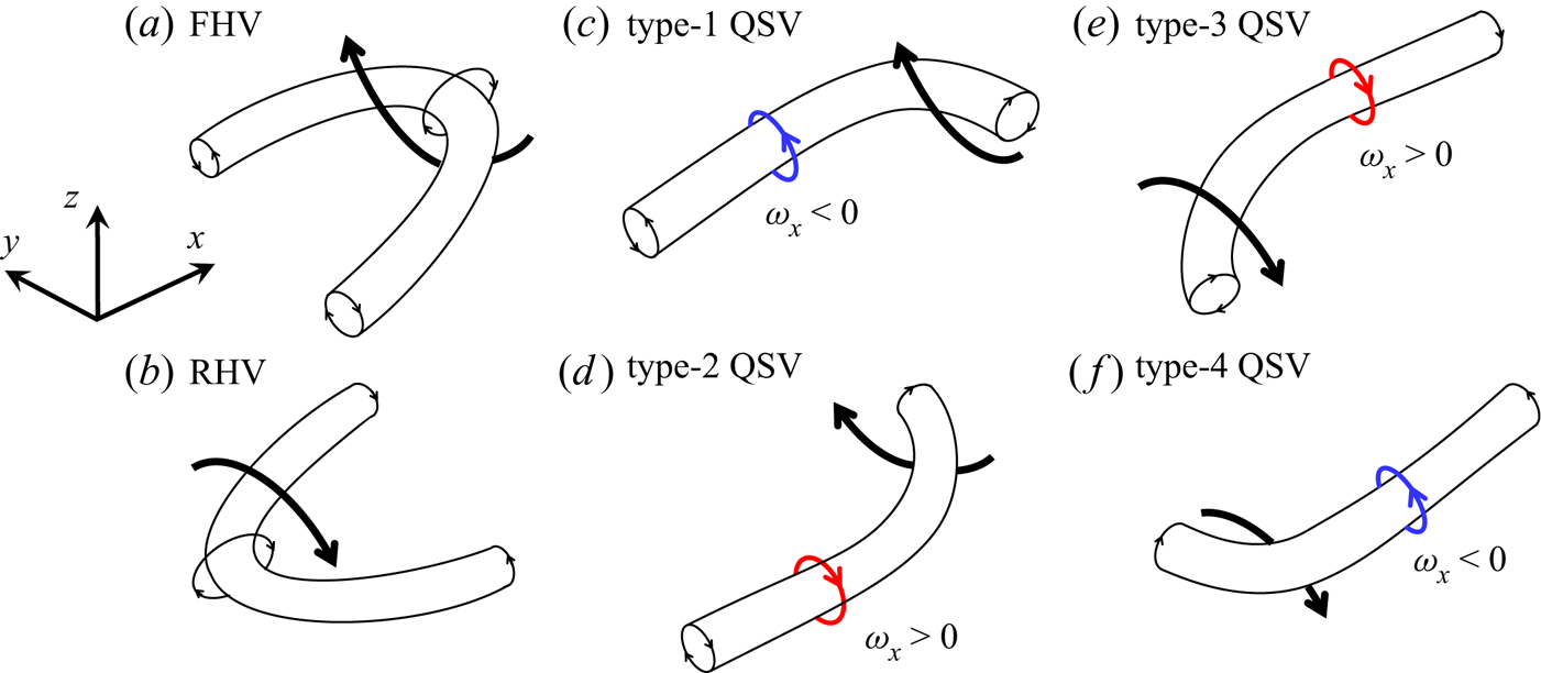
With the identification and classification scheme, the population partitions of different types of CVSs and their spatial variations can then be quantified by computing the cumulative occurrence count that a spatial coordinate  $(x,z^+)$ is occupied by one of the three types of CVSs, as shown in figure 13 for the flows of cases I0 and L0. The distributions are ensemble results computed from the flows beneath four surface waves at 21 independent time instances. The corresponding histogram variations in wave phase
  $\phi$, which are calculated by summing up the occurrence counts over
  $z^+$, are also shown in figure 13. Comparing the distributions of cases I0 and L0 reveals that more CVSs form beneath steeper waves, consistent with the qualitative observation from figure 11.
Spatial distributions of the CVSs in the simulated flows of I0 (a–d) and L0 (e–h). The two panels in the top two rows are distributions of accumulative occurrence count of characteristic vortices of FHV (a,e), RHV (b,f) and QSV (c,g), respectively. The bottom panels (d,h) are the corresponding histogram variations in wave phase  $\phi$. The wave trough and the wave crest are defined to be
  $0^{\circ }$ and
  $180^{\circ }$, respectively.

Similar to the turbulent airflow above the wavy surface (Chen et al. Reference Chen, Tsai, Druzhinin and Troitskaya2020), the distributions of the CVSs in the turbulent aqueous flows beneath surface waves also strongly depend on the wave phase. The QSVs dominate the distribution, but in contrast to airflow, the populations of FHV and RHV are insignificant. The QSVs are observed beneath the entire wavy surface; the distribution initiates near the wave crest ( $x / \lambda \cong 0.5$ in figure 13(c,g), and extends upstream along the windward face
  $(0 < x/\lambda < 0.5)$, subducts below the wave trough
  $(x / \lambda =0)$ and continues toward the next forward face
  ${(0.5 < x/\lambda < 1)}$. The peak of the occurrence-count histogram is located near the middle of the windward face (
 $\theta \cong 90^{\circ }$ in figure 13d,h).
The corresponding distributions of the four types of QSVs are shown in figure 14. Again, type-3 and 4 QSVs, which can be considered as incomplete or degenerate RHVs with elongated vortices bending inward at the submerged upstream end, significantly outgrow type-1 and 2 QSVs.
Spatial distributions of accumulative occurrence count of four types of QSVs for the simulated flows of I0 (a–d) and L0 (e–h).

The above analyses reveal that type-3 and type-4 QSVs accumulate beneath the backward surface of the carrier wave and dominate the formation of CVSs. Figures 11(d)–11(e) depict the instantaneous skeleton distributions of QSVs for the corresponding distributions of  $\lambda _{ci}^2$ isosurfaces shown in figures 11(a)–11(b), indicating the QSVs are more populous along several elongated regions; and the QSVs with positive and negative streamwise vorticities tend to align alternatively.
Comparing the QSVs distributions in figures 11(a) and 11(d) with the corresponding surface temperature distributions in figure 6(b) further reveals that the accumulation regions of QSVs roughly coincide with predominant streaks. This can also be demonstrated by examining the transverse distance  $d_k$ between the skeleton of the QSV and the nearest skeleton of the predominant streak depicted in figure 7(b). Figure 15 presents the probability density histograms
  $\mathcal {P}$ and their corresponding cumulative probability distributions
  $\mathcal {C}_{\mathcal {P}}$ of the non-dimensional distance
  $d^+_k={d_k}u_*/\nu$ for the identified QSV skeletons in the simulated flows of cases I0 and L0. The results reveal that approximately
  $50\,\%$ of the QSVs are within the interval of 30 wall units from the predominant streaks.
Probability density histograms (red vertical bars) and cumulative probability distributions (black lines and rectangular symbols) of the non-dimensional distance  $d^+_k$ from the skeleton of the QSV to the nearest skeleton of the predominant streak for the flows of cases I0 (a) and L0 (b).

The above observations suggest that the spanwise heterogeneity of the QSV distribution could be attributed to the larger-scale circulatory structure of LCs. In § 6, the averaged spatial relation between QSV and LC, and the interplay between these two vortical structures are examined.
6. Enhancement of QSVs by LCs
6.1. Variable-interval space averaging of QSVs
To explore the relative spatial locations of the fine-scale QSVs and the large-scale Langmuir cells, the method of variable-interval space averaging (VISA, e.g. Kim & Moin Reference Kim and Moin1986) is combined with the CVS eduction and classification scheme described in § 5. The modified VISA procedure consists of two major steps.
First, the QSVs of the designated type whose skeletons intersect with the plane of  $z_0^+ = h(1-\zeta _0)u_*/\nu \cong 13.23$ are identified. The vertical coordinate
  $\zeta _0\cong 1-13.23\nu /(h u_*)$, where a layer of discretized points is located in the computational domain, is around the skeleton midpoints of most QSVs;
  $\zeta _0$ is chosen by experimenting with various values to produce the best averaging result. The intersection-point coordinate of the
  $i$th QSV skeleton is denoted by
  $(x_{0_i}, y_{0_i}, \zeta _0)$. A realization interval encompassing the identified QSV is defined by choosing a rectangular domain centred horizontally at
  $(x_{0_i}, y_{0_i})$.
Aligning  $(x_{0_i}, y_{0_i}, \zeta _0)$ of the identified intervals, averaging of the velocity field of the realized QSV events is then taken as
 \begin{equation} \{\boldsymbol{\upsilon}\}({X},\varUpsilon,\zeta) = \frac{1}{N_t N_s} \sum_{n=1}^{N_t} \sum_{i=1}^{N_v} \boldsymbol{\upsilon} \left( x-x_{0_i}, y-y_{0_i}, \zeta, t_n \right), \end{equation}
where  $N_v$ is the total number of realizations of QSVs,
  $N_t$ is the total number of ensemble time instances,
  $({X}=0,\varUpsilon =0,\zeta =0)$ is the origin of the averaging interval. The VISA velocity field
  $\{\boldsymbol {\upsilon }\}$ is analysed to educe the flow structures.
Since type-3 and 4 QSVs dominate the population of educed CVSs, as shown in figure 14, the flow intervals encompassing these two types of CVSs are realized. Figure 16 depicts the plane distributions of the averaged velocities ( $\{u'\},\{\upsilon '\},\{w'\}$) and the isosurface
  $\lambda _{ci}^2=0.06$ from different perspective views of case I0, delineating the dominant flow pattern and vortical structure around QSVs. The results deduced from the realizations of type-3 and 4 QSVs are presented in the right and left columns, respectively. The ensemble averaging is taken from flows at 21 time instances from
  $t=25T_0$ to
  $30T_0$ of the simulation.
The distributions of the velocities from different perspective views for the VISA flow of case I0 ( $ak=0.22$). The averaged QSVs are revealed by the isosurface
  $\lambda _{ci}^2=0.06$. The red and blue colours of the isosurfaces represent the vortical structures with positive and negative streamwise vorticities, respectively. The results deduced from the realizations of type-3 and 4 QSVs are shown in (e–h) and (a–d), respectively. The coordinates are made non-dimensional by the friction length. The ensemble averaging is taken from flows at 21 time instances from
  $t=25T_0$ to
  $30T_0$ of the simulation.
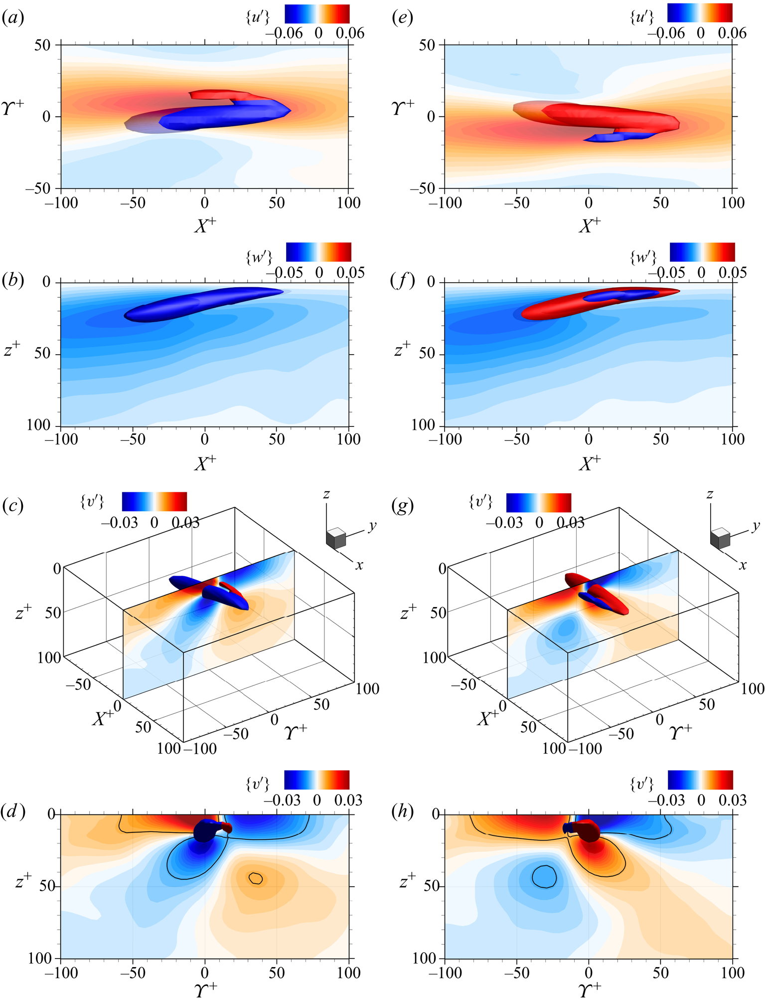
The  $\lambda _{ci}^2$ isosurfaces highlight the characteristic geometries of type-3 and 4 QSVs: both averaged vortical structures elongate in the streamwise direction from the submerged
  $(z^+ \cong 25)$ upstream head to the near-surface downstream end. The averaged structures do not have the submerged spanwise heads; the lengths are shorter than the observed QSVs of the instantaneous flow field in figure 11. These are attributed to the smearing effect of averaging, particularly near the two ends of the QSVs. The averaged structure deduced from the realizations of type-4 QSV (see figure 16a–d) is dominated by an elongated structure of
  $\{\omega _x\} < 0$ that forms on the right edge (looking downstream,
  $\varUpsilon < 0$) of a streamwise high-speed streak. A degenerated structure of
  $\{\omega _x\} > 0$ is attached to the downstream end of the dominant
  $\{\omega _x\} < 0$ structure and extends toward the left side of the streak. This is due to the coexistence of some type-4 QSVs on the other side of the dominant streaks (
 $\varUpsilon > 0$). A similar but opposite-orientation pattern of vortical structure is observed in the averaged flow based on realizations of the type-3 QSV (figure 16e–h). These results reveal two distinct features of the QSV structures: first, the type-3 and 4 QSVs form at different but preferable spanwise and vertical locations relative to the Langmuir cells. Second, the type-3 and 4 QSVs do not appear simultaneously in the averaged flow, suggesting the intermittent appearances of the two types of QSVs along both sides of the predominant streaks in the instantaneous flow field.
Both averaged velocity fields based on realizations of type-3 and 4 QSVs reveal flow patterns similar to that of averaged LCs depicted in figure 8: a streak with higher streamwise velocity forms on the water surface, the near-surface flows converge toward the surface streak, downward beneath the surface streak, and diverge in the submerged depth. However, in contrast to the averaged flow of LC, the averaged flow based on QSV realization exhibits spanwise unbalance. For averaging based on type-4 QSV realizations (figure 16d), the flow structure on the opposite side of the QSV  $(\varUpsilon > 0)$ remains analogous to that of LCs in figure 8; the near-surface convergence
  $(\{\upsilon '\} > 0)$ above the QSV and the submerged divergence
  $(\{\upsilon '\} < 0)$ beneath the QSV, however, are more intensified and skewed toward the type-4 QSV. An opposite unbalanced flow pattern is observed for averaging based on type-3 QSV realization (figure 16h). Such averaged flow structures again imply that in the instantaneous flow field, the vortical structures of
  $\omega _x > 0$, primarily type-3 QSVs, tend to form on the port side of the dominant thermal streaks. Likewise, the major vortical structures that appear on the starboard side of the dominant streaks are mainly type-4 QSVs with
  $\omega _x < 0$. Therefore, the resulting averaged flow beneath a dominant streak is formed by a localized swirling flow of either type-3 or 4 QSV superimposed on the larger-scale flow of LCs, as illustrated by the schematics in figures 17(a) and 17(b). Of note is that QSVs can also be observed in the region away from the predominant streaks, as revealed in figures 11 and 15. These QSVs are perhaps formed by the same mechanism as that in wall turbulence.
(a,b) Schematics of vortical structures near Langmuir cells viewing downstream. The counter-rotating circulatory pair denotes the Langmuir cells. The dark-red colour beneath the origin of the  $\varUpsilon -z$ axes represents the high-speed surface jet; the wind is in the direction out of the paper. The type-4 and 3 QSVs are depicted by blue and red circles in (a,b), respectively. (c) Schematic of a perturbed streak between the counter-rotating Langmuir cells.
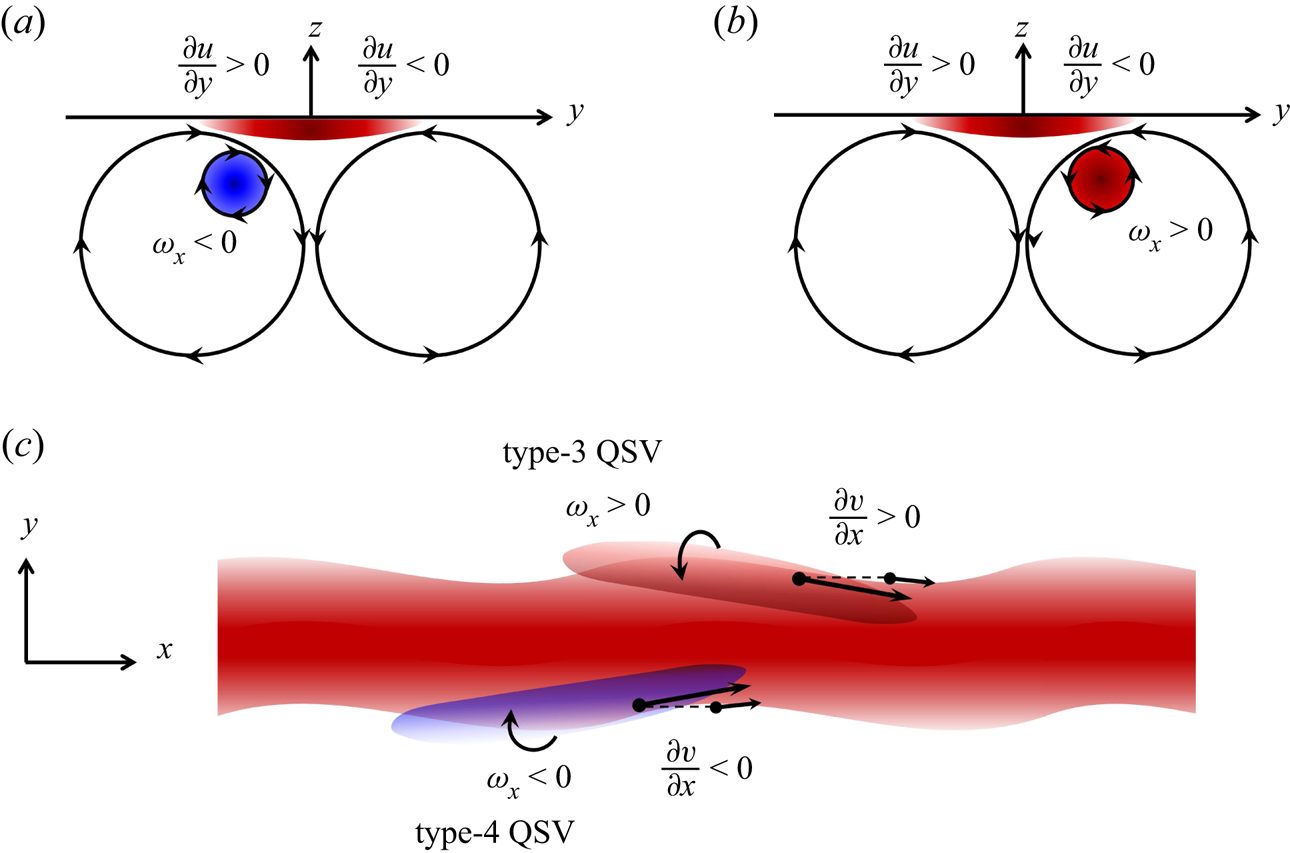
Figure 18 presents the plane distributions of the velocities and the isosurface  $\lambda _{ci}^2 = 0.06$ for the averaged flow of case L0 (
 $ak=0.135$). The averaged velocity distributions and vortical structure of L0 are similar to those of I0 (
 $ak=0.22$). However, decreasing the steepness of the carrier surface waves weakens the strength of the QSVs; the length of the averaged QSV and the maximum averaged velocities decrease. This observation indicates that the attenuation of LCs attributed to decreasing wave steepness weakens the formation of QSVs in the vicinity of LCs, inferring the role of LCs in enhancing the nearby QSVs.
The distributions of the velocities from different perspective views for the VISA flow of case L0 ( $ak=0.135$). The averaged QSVs are revealed by the isosurface
  $\lambda _{ci}^2=0.06$. The red and blue colours of the isosurfaces represent the vortical structures with positive and negative streamwise vorticities, respectively. The results deduced from the realizations of type-3 and 4 QSVs are shown in (e–h) and (a–d), respectively. The coordinates are made non-dimensional by the friction length. The ensemble averaging is taken from simulated flows at 21 time instances from
  $t=30T_0$ to
  $35T_0$ of the simulation.

The above observations validate the proposition raised in § 3 regarding how the steepness of surface waves affects the distribution of surface streak spacings in Langmuir turbulence: the interaction between the surface waves and the shear layer gives rise to the LCs that enhance the formation of QSVs. The QSVs are more populous in the vicinity of LCs, resulting in finer streak spacing. Increasing the steepness of the surface waves strengthens the LCs, thus intensifying the enhancement of LCs on the QSVs. Such a trend is consistent with the finding revealed in the probability distributions of streak spacing shown in figure 5 and the distributions of CVSs presented in § 5.2. The observation sheds light on understanding the wind wave–turbulence interaction by revealing another route of energy transport from surface waves to turbulence. The recent study by Xuan et al. (Reference Xuan, Deng and Shen2020) also highlighted such a wave–turbulence energy transport route.
6.2. Enhanced formation of QSVs by LCs
The spatial correlation between the Langmuir cells and the nearby type-3 and 4 QSVs observed in the previous section indicates the possible interaction between the LCs and the QSVs. The various production budgets of streamwise enstrophy  $\varOmega _x = 0.5\omega _x^2$ in the vorticity transport attributed to the flow field is then examined to elucidate such an interaction.
Applying the decomposition (2.2) to the velocity and vorticity fields, and noting that the flow set-up of long-crest waves renders the decomposed components of velocity and vorticity as  $u=\bar {u}(z,t)+\tilde {u}(x,z,t)+u'(x,y,z,t)$,
  $\upsilon \approx \upsilon '(x,y,z,t)$,
  $w\approx \tilde {w}(x,z,t)+w'(x,y,z,t)$,
  $\omega _x\approx \omega '_x(x,y,z,t)$,
  $\omega _y=\bar {\omega }_y(z,t)+\tilde {\omega }_y(x,z,t)+\omega '_y(x,y,z,t)$ and
  $\omega _z\approx \omega '_z(x,y,z,t)$, the transport equation of streamwise enstrophy
  $\varOmega _x$ is expressed as
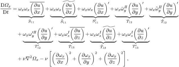 \begin{align} \frac{{\rm
D}\varOmega_x}{{\rm D}t} &= \underbrace{\omega_x \omega_x
\overline{\left( \frac{\partial u}{\partial x}
\right)}}_{\bar{S}_{11}} + \underbrace{\omega_x \omega_x \!\widetilde{\,\left( \frac{\partial u}{\partial x}\right)\,}}_{\tilde{S}_{11}}\! +\underbrace{\omega_x \omega_x
{\left( \frac{\partial u}{\partial x} \right)'}}_{S'_{11}}
+\underbrace{\omega_x \bar{\omega}^{I\!I}_y
{\left(\frac{\partial u}{\partial
y}\right)'}}_{\bar{T}_{12}} +\underbrace{\omega_x
\tilde{\omega}^{I\!I}_y {\left(\frac{\partial u}{\partial
y}\right)'}}_{\tilde{T}_{12}} \nonumber\\
&\quad +\underbrace{\omega_x \omega'^{I\!I}_y
{\left(\frac{\partial u}{\partial y}\right)'}}_{T'_{12}}
+\underbrace{\omega_x \omega_z^I \overline{\left(
\frac{\partial u}{\partial z} \right)}}_{\bar{T}_{13}}
+\underbrace{\omega_x \omega_z^I \widetilde{\left(
\frac{\partial u}{\partial z} \right)}}_{\tilde{T}_{13}}
+\underbrace{\omega_x \omega_z^I {\left( \frac{\partial
u}{\partial z} \right)'}}_{T'_{13}} \nonumber\\ &\quad +\nu
{\nabla}^2 \varOmega_x - \nu \left[ {\left( \frac{\partial
\omega_x}{\partial x} \right)}^2 + {\left( \frac{\partial
\omega_x}{\partial y} \right)}^2 + {\left( \frac{\partial
\omega_x}{\partial z} \right)}^2 \right],
\end{align}
\begin{align} \frac{{\rm
D}\varOmega_x}{{\rm D}t} &= \underbrace{\omega_x \omega_x
\overline{\left( \frac{\partial u}{\partial x}
\right)}}_{\bar{S}_{11}} + \underbrace{\omega_x \omega_x \!\widetilde{\,\left( \frac{\partial u}{\partial x}\right)\,}}_{\tilde{S}_{11}}\! +\underbrace{\omega_x \omega_x
{\left( \frac{\partial u}{\partial x} \right)'}}_{S'_{11}}
+\underbrace{\omega_x \bar{\omega}^{I\!I}_y
{\left(\frac{\partial u}{\partial
y}\right)'}}_{\bar{T}_{12}} +\underbrace{\omega_x
\tilde{\omega}^{I\!I}_y {\left(\frac{\partial u}{\partial
y}\right)'}}_{\tilde{T}_{12}} \nonumber\\
&\quad +\underbrace{\omega_x \omega'^{I\!I}_y
{\left(\frac{\partial u}{\partial y}\right)'}}_{T'_{12}}
+\underbrace{\omega_x \omega_z^I \overline{\left(
\frac{\partial u}{\partial z} \right)}}_{\bar{T}_{13}}
+\underbrace{\omega_x \omega_z^I \widetilde{\left(
\frac{\partial u}{\partial z} \right)}}_{\tilde{T}_{13}}
+\underbrace{\omega_x \omega_z^I {\left( \frac{\partial
u}{\partial z} \right)'}}_{T'_{13}} \nonumber\\ &\quad +\nu
{\nabla}^2 \varOmega_x - \nu \left[ {\left( \frac{\partial
\omega_x}{\partial x} \right)}^2 + {\left( \frac{\partial
\omega_x}{\partial y} \right)}^2 + {\left( \frac{\partial
\omega_x}{\partial z} \right)}^2 \right],
\end{align}
where the spanwise and vertical vorticities are expressed as  $\omega _y = \partial u/\partial z - \partial w/\partial x \equiv \omega _y^I + \omega _y^{I\!I}$ and
  $\omega _z = \partial \upsilon /\partial x-\partial u/\partial y \equiv \omega _z^I + \omega _z^{I\!I}$. In deriving (6.2), the contributions of vorticity
  $\omega ^{I}_y$ to the budget, namely the terms associated with
  $(\partial u/\partial z)(\partial u/\partial y)$, cancel out the contributions of
  $\omega ^{I\!I}_z$, namely the terms associated with
  $-(\partial u/\partial y)(\partial u/\partial z)$ (Brooke & Hanratty Reference Brooke and Hanratty1993). Therefore the component of vertical vorticity
  $\omega _z^{I\!I}=-\partial u/\partial y$ makes no net contribution to the production budget, highlighting the impact of the flow process that induces the vertical vorticity component
  $\omega ^I_z=\partial \upsilon /\partial x$. To present the actual contribution of the wave motion, only the variation along the wave-following coordinate
  $\xi$ is considered in evaluating the derivatives of
  $x$ and
  $y$ of streamwise velocity. In (6.2), the first three terms
  $\bar {S}_{11}$,
  $\tilde {S}_{11}$ and
  $S'_{11}$ represent the production of
  $\varOmega _x$ due to the stretching of
  $\omega _x$ by mean, wave straining and fluctuating streamwise variation of the streamwise velocity, respectively;
  $\bar {T}_{12}$,
  $\tilde {T}_{12}$ and
  $T'_{12}$ represent the production of
  $\varOmega _x$ attributed to the turning of spanwise vorticity,
  $\bar {\omega }^{I\!I}_y$,
  $\tilde {\omega }^{I\!I}_y$ and
  $\omega '^{I\!I}_y$, by fluctuating spanwise variation of the streamwise velocity, respectively;
  $\bar {T}_{13}$,
  $\tilde {T}_{13}$ and
  $T'_{13}$ are the productions of
  $\varOmega _x$ due to the tilting of vertical vorticity
  $\omega ^{I}_z=\partial \upsilon /\partial x$ by mean, wave straining and fluctuating vertical variation of the streamwise velocity, respectively; the last two terms are viscous diffusion and dissipation, respectively.
Note that Lu et al. (Reference Lu, Tsai, Garbe and Jähne2021) explained the impact of surface waves on the scaling of streak spacing by comparing the difference in enstrophy transport beneath the gravity–capillary waves and a flat surface without knowing the interaction mechanism between the LC vortical structures and QSVs in Langmuir turbulence. We reappraise the analysis of streamwise enstrophy transport in Lu et al. (Reference Lu, Tsai, Garbe and Jähne2021) to validate the interaction process depicted in figure 17 and described above. The analysis is similar to that in Lu et al. (Reference Lu, Tsai, Garbe and Jähne2021), but the interpretations are new.
Figure 19 presents the phased-averaged distributions of the production terms in the enstrophy transport equation (6.2) for the simulated flow of case I0. For comparison, the distributions of the total production budget  $S_{11}+T_{12}+T_{13}$, the production budget by turning
  $T_{12}$ and the production budget by tilting
  $T_{13}$ are also depicted in figures 19(j), 19(k) and 19(l), respectively, where
  $S_{11}=\bar {S}_{11}+\tilde {S}_{11}+S'_{11}$,
  $T_{12}=\bar {T}_{12}+\tilde {T}_{12}+T'_{12}$ and
  $T_{13}=\bar {T}_{13}+\tilde {T}_{13}+T'_{13}$. The distributions on the
  $x-z$ plane are obtained by taking the phase average (2.5). The corresponding vertical variations of the gross contributions by the various terms are shown in figures 20(a)–20(c). The gross contribution is computed by taking the spatial average (2.3).
Phase-average distributions of various production terms in the transport equation of enstrophy  $\varOmega _x$ for the flow of case I0; (a)
  $\bar {S}_{11}$, (b)
  $\bar {T}_{12}$, (c)
  $\bar {T}_{13}$, (d)
  $\tilde {S}_{11}$, (e)
  $\tilde {T}_{12}$, (f)
  $\tilde {T}_{13}$, (g)
  $S'_{11}$, (h)
  $T'_{12}$, (i)
  $T'_{13}$, (j)
  $S_{11}+T_{12}+T_{13}$, (k)
  $T_{12}$ and (l)
  $T_{13}$. The distributions are ensemble results computed from the flows under four carrier waves at 21 independent time instances from
  $t=25T_0$ to
  $30T_0$.
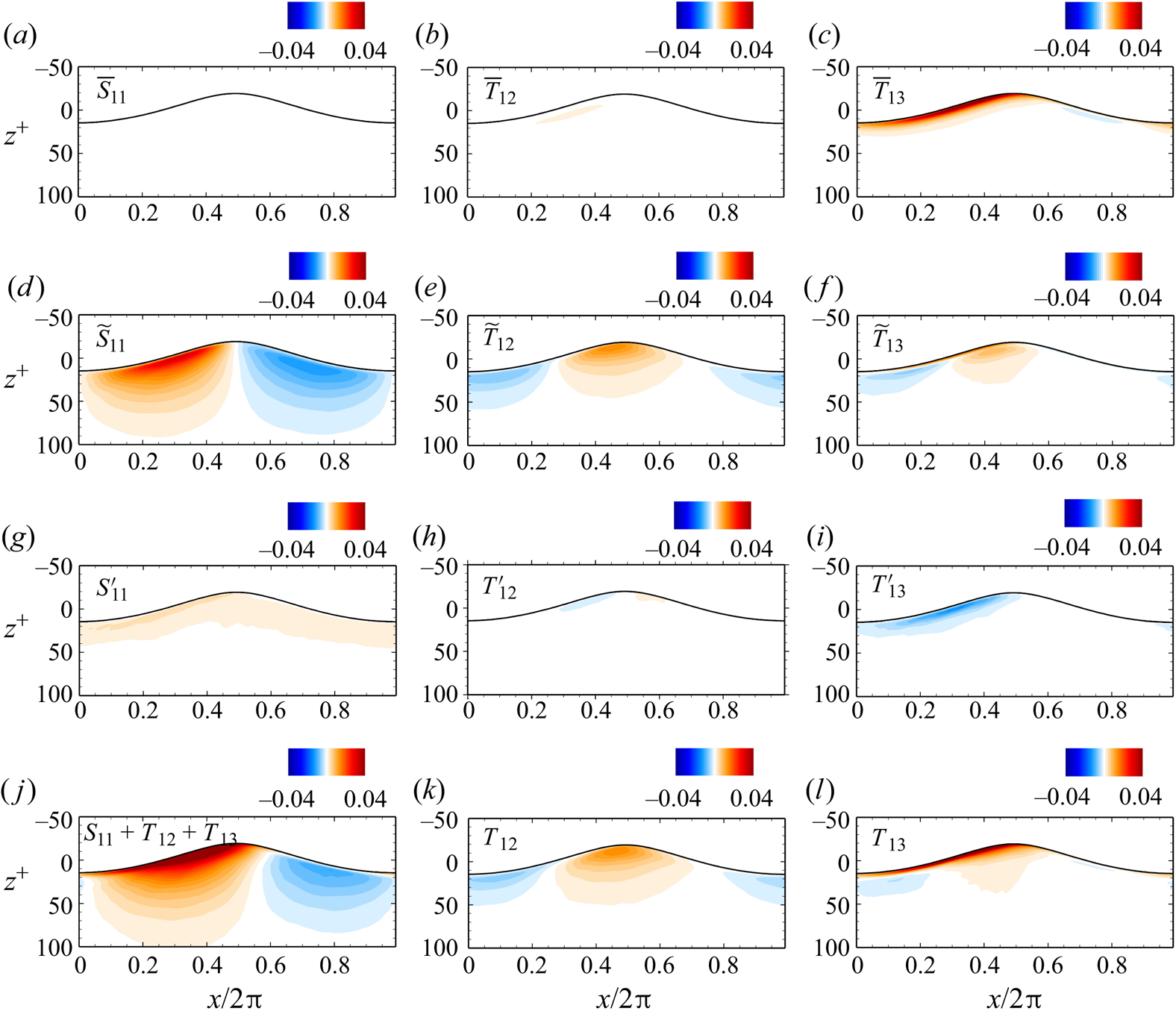
Vertical variations of various enstrophy  $\varOmega _x$ production terms averaged over the
  $\xi$–
 $\psi$ plane for flows of cases I0 (upper row, a–c) and L0 (lower row, d–f);
  $S_{11}=\bar {S}_{11}+\tilde {S}_{11}+S_{11}'$,
  $T_{12}=\bar {T}_{12}+\tilde {T}_{12}+T_{12}'$ and
  $T_{13}=\bar {T}_{13}+\tilde {T}_{13}+T_{13}'$.
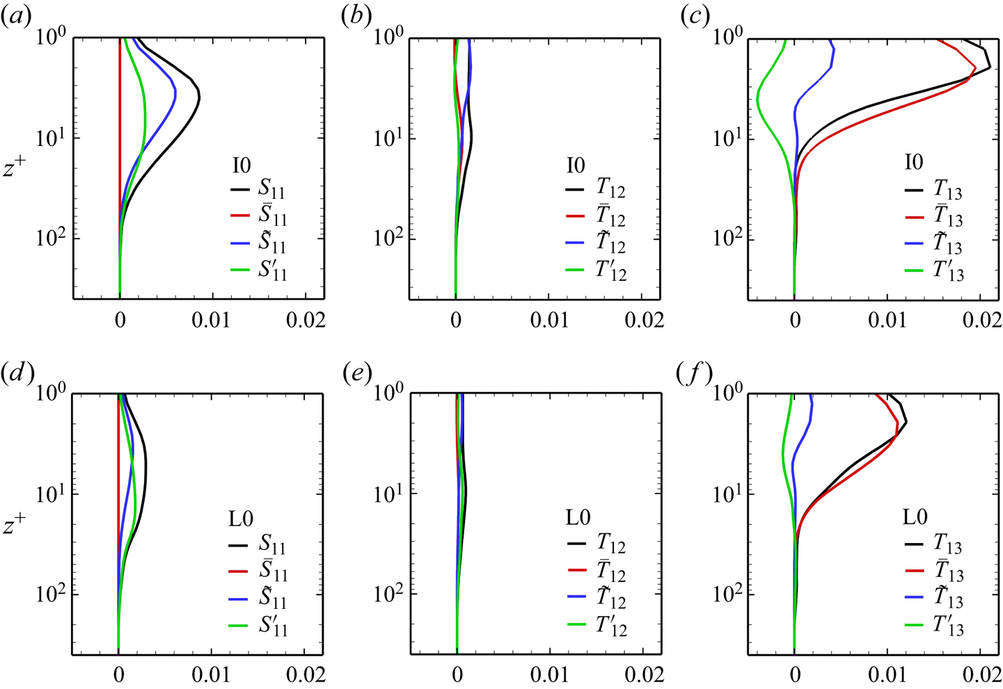
The profiles of the gross contributions in figure 20 indicate that the most significant production to the streamwise enstrophy is contributed by the  $\bar {T}_{13}$ term. This production occurs within the layer beneath the windward surface, as shown in figure 19(c). This is also the region where the QSVs accumulate, as depicted in figures 13 and 14. The VISA results of figures 16 and 18 further reveal that the QSVs tend to form in the edge vicinity of the surface streaks induced by the LCs, with small tilting and turning angles relative to the streaks. These observations, therefore, suggest the following interaction process between the QSVs and the streaks in enhancing streamwise enstrophy production. A schematic helping explain the process is depicted in figure 17(c).
Suppose that the background flow is turbulent such that the fluctuations act over time scales that are small with respect to the LCs, and the QSVs have somehow formed to realize the respective velocity fields of LCs and mean shear flow. The counter-rotating cells of LCs induce high-speed streamwise streaks in the near-surface region and introduce spanwise gradient of the streamwise velocity  $\partial u/\partial y<0$ and
  $\partial u/\partial y>0$ on the port and starboard sides of the streaks, respectively, as illustrated in the schematics of figures 17(a) and 17(b). The QSVs in the edge vicinity of the streak, of which the downstream near-surface portions tilt upward and turn toward the streak, perturb the nearby flows. Specifically, the type-3 QSV, which tends to form on the port side of the streak, induces
  $\partial \upsilon /\partial x=\omega _z^I>0$ in the flow region above the upper part of the QSV, as depicted in figure 17(c). Similarly, the type-4 QSV on the starboard side of the streak induces
  $\partial \upsilon /\partial x<0$. The vertical vorticity in these localized regions is tilted by vertical shear through
  $\omega _x\omega _z^I \overline {(\partial u/\partial z)}$ and therefore contribute to the production of streamwise enstrophy.
To validate the above proposition regarding the production process of streamwise enstrophy arising from the interaction between the QSVs and the LC streak, we present in figure 21 the distributions of related flow properties in the VISA flows around the QSVs. The distributions of the spanwise gradient of streamwise velocity clearly show that type-3 and 4 QSVs form on the port ( $\{\partial u'/\partial y\}>0$) and starboard (
 $\{\partial u'/\partial y\}<0$) sides of the streaks, respectively; they also reveal the streaks being undulated to be parallel with the QSVs. Consequently, strong streamwise gradient of spanwise velocity occurs in a localized region around the near-surface part of the QSVs, as shown in figures 21(b) and 21(f). The resulting contribution to the production
  $\omega _x (\partial \upsilon /\partial x)\overline {(\partial u/\partial z)}$ is depicted in figures 21(d) and 21(h). Note that such a production process is not observed in the flow regions near the streaks without the QSVs, therefore underlining the interaction between the QSVs and LCs.
The distributions of  $\{-\partial u'/\partial y\}$ (a,e),
  $\{\partial \upsilon /\partial x\}$ (b,f),
  $\{\omega _x\}$ (c,g) and
  $\{\omega _x\}\{\partial \upsilon /\partial x\}$ (d,h) at
  $z^+=3.29$ for the VISA flow of case I0. The averaged QSVs are revealed by the isosurfaces
  $\lambda _{ci}^2=0.06$. The red and blue colours of the isosurfaces represent the vortical structures with positive and negative streamwise vorticities, respectively. The results deduced from the realizations of type-3 and 4 QSVs are shown in the right and left columns, respectively. The coordinates are made non-dimensional by the friction length. The ensemble averaging is taken from simulated flows at 21 time instances from
  $t=25T_0$ to
  $30T_0$ of the simulation.
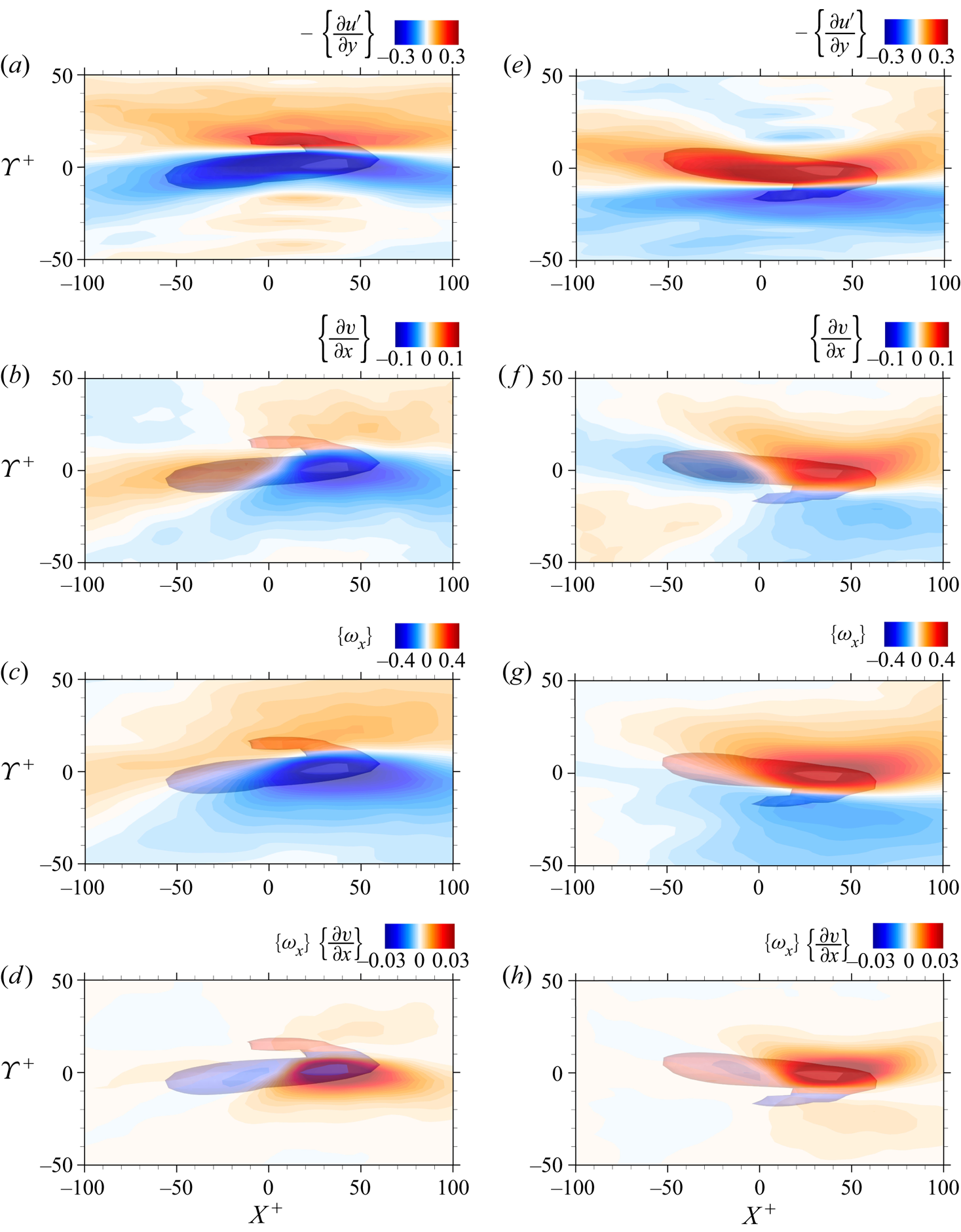
The distribution of  $\bar {T}_{13}$ production initiates from the wave crest and extends upstream in the layer beneath the windward surface. In the same region, stretching production due to wave straining,
  $\tilde {S}_{11}$, is also significant, as shown in figure 19(d). The combined effect of these two mechanisms intensifies the production of streamwise enstrophy and enhances the formation of QSVs there. These QSVs are convected upstream in the
  $-x$-direction relative to the wave (Xuan et al. Reference Xuan, Deng and Shen2019), and accumulate in the surface layer extending from the windward surface to the wave trough, as revealed by the spatial distributions of accumulative occurrence count of QSVs depicted in figure 13(c), and figures 14(c) and 14(d). Beneath the leeward surface, compression straining of wave results in negative production of streamwise enstrophy,
  $\tilde {S}_{11}<0$. However, the gross contribution of
  $\tilde {S}_{11}$ is positive, as shown in in figure 20(a), indicating the wave stretching is more significant than the wave compression in the production of streamwise enstrophy.
The vertical profiles of the gross contributions to streamwise enstrophy by various mechanisms for the flow of case L0 are presented in figures 20(d)–20(f). Comparing the results of I0 and L0 reveals that decreasing the steepness of the surface wave reduces all the contributions to the production of streamwise enstrophy, in particular, the  $\tilde {S}_{11}$ and
  $\bar {T}_{13}$ terms. Reduction in the contribution attributed to stretching/compression of wave straining (
 $\tilde {S}_{11}$ term) is evident since the streamwise velocity associated with wave motions (
 $\tilde {u}$) decreases with the steepness
  $ak$. Reducing the wave steepness also decreases the Stokes drift and attenuates the LCs and the accompanying streaks. This weakens the interaction between the streaks and the nearby QSVs, consequently decreasing the production owing to the interaction (
 $\bar {T}_{13}$ term).
7. Conclusions
Direct numerical simulations of turbulent shear flow beneath stress-driven surface waves are conducted to reveal the underlying vortical structures associated with LCs and turbulent QSVs, and their mutual interaction. Both vortical structures manifest themselves by inducing wind-aligned streaks on the wavy surface. However, the length scales and the footprint intensities of both streaks are different. This allows for decomposing of the streaks according to their characteristic signatures. Guided by the decomposed surface imageries, the flow intervals beneath the predominant streaks are realized to educe the responsible averaged flow structure. The result reveals a cellular structure consistent with the counter-rotating circulatory pair of LCs. Linear instability analysis of the wave-averaged CL equations is then conducted to determine whether the least stable spanwise spacings given by instability theory are consistent with our LC spacing found numerically. The spanwise wavelengths of the most unstable disturbances are found to be close to the width of averaged LC pairs. The favourable comparison also confirms the effectiveness of the developed decomposition method in extracting surface imageries associated with physical processes underneath.
We isolate the CVSs using a detection criterion based on conjugate complex eigenvalues of the velocity-gradient tensor and classify the vortical structures according to the topological characteristics of their skeletons. The results indicate that QSVs, which can be considered to be the degenerated reversed horseshoe vortices, dominate the population of identified CVSs. These QSVs accumulate beneath the windward surface. Moreover, the QSVs are more populous in the vicinity of the streamwise streaks formed by the LCs, suggesting such spanwise heterogeneity could be attributed to the circulatory structures of the LCs.
To understand the spatial correlation between the LCs and the QSVs, the VISA technique is utilized in the regions around the identified QSVs. The averaged flows reveal that the CVSs that tend to form on the port side of the streamwise streaks induced by the LCs are type-3 QSVs with positive streamwise vorticity. In contrast, the CVSs on the starboard side edge of the surface streaks are more likely to be type-4 QSVs with negative streamwise vorticity. The type-3 and 4 QSVs do not form concurrently on both sides of the streaks. The downstream near-surface portions of these QSVs tilt upward and turn toward the streaks. Such a spatial configuration between the QSVs and the streaks disturbs the nearby flows of the LCs and undulates the streaks to be parallel with the QSVs. The staggered type-3 and 4 QSVs in the edge vicinity of the streaks induce streamwise gradient of the spanwise velocity, that is, vertical vorticity, in the localized regions around the near-surface parts of the QSVs. The vertical shear tilts the vertical vorticity of these flow regions, contributing to streamwise enstrophy production and enhancing the formation of QSVs.
The denser distribution of QSVs in the vicinity of Langmuir cells also implies more fine streaks being formed near the predominant streaks attributed to LCs, resulting in smaller spacings between streaks than those away from the predominant streaks. Thus the distribution of the scaled streak spacings  $d^+$ deviates from the log-normal distribution, and the mean value
  $\overline {d^+}$ becomes smaller than 100. The deviation becomes more significant as the steepness of surface waves increases, which is consistent with the intensification of LCs.
These findings from numerical simulations explain the reduction of mean streak spacings on the infrared images of non-breaking wind waves observed in the laboratory experiments (figure 2). They also highlight the differences in the vortical structures between the Langmuir turbulence and the turbulent wall layer.
Acknowledgements
The authors would like to thank T.-W. Wang for helping process some of the data and L.-A. Hsieh for helping conduct the stability analysis of the CL equations.
Funding
This study was supported by the Taiwan National Science and Technology Council through grants 110-2611-M-002-010 (WTT), 111-2611-M-002-013 (WTT) and 110-2811-M-002-554 (GHL).
Declaration of interests
The authors report no conflict of interest.
Appendix A. Decomposition of surface image
The image processing method developed in Lu et al. (Reference Lu, Tsai and Jähne2019) is an extension of the two-dimensional ensemble empirical mode decomposition (EEMD) of Wu et al. (Reference Wu, Huang and Chen2009). Employing the EEMD algorithm of Huang et al. (Reference Huang, Shen, Long, Wu, Shih, Zheng, Yen, Tung and Liu1998) and grouping the intrinsic mode functions (IMFs) according to their distinct directionalities, a data image  $\theta (x,y)$ is first decomposed as
 \begin{equation} \theta(x,y)= \sum_{k=1}^M\tilde{\theta}_k(x,y) + \sum_{k=1} \check{\theta}_k(x,y) \equiv \theta_{\mathcal{W}}(x,y)+\theta_{\mathcal{V}}(x,y), \end{equation}
where  $\tilde {\theta }_k$ and
  $\check {\theta }_k$ are the derived IMFs with the dominant signatures aligned with the spanwise and streamwise directions. For a surface image of wind waves,
  $\theta _\mathcal {W}$ and
  $\theta _\mathcal {V}$, are the decomposed images associated with the surface waves and the streaks, respectively.
The derived wave-correlated and streak-correlated IMFs,  $\tilde {\theta }_k$ and
  $\check {\theta }_k$, show a trend of increasing spatial scale with
  $k$. They are further decomposed into groups based on the distinct length scales of the surface signatures as
 \begin{equation} \theta (x,y) = \theta_{\mathcal{W}_G} (x,y) + \theta_{\mathcal{W}_C} (x,y) + \theta_{\mathcal{V}_{LC}} (x,y) + \theta_{\mathcal{V}_T} (x,y), \end{equation}
where  $\theta _{\mathcal {W}_G}$,
  $\theta _{\mathcal {W}_C}$,
  $\theta _{\mathcal {V}_{LC}}$ and
  $\theta _{\mathcal {V}_T}$ are the decomposed images predominantly associated with the long gravity waves, the short capillary waves, the wind-aligned streaks attributed to LCs and the quasi-streamwise streaks associated with turbulent QSVs, respectively. The criterion for differentiating the derived IMF is based on the intrinsic length scales of the flow processes observed in the experimental measurements. Lu et al. (Reference Lu, Tsai and Jähne2019) conducted a detailed sensitivity test of the criteria in classifying the derived IMFs of infrared images taken at various wind-wave conditions. The results show the ranges of decomposition criteria in which the decomposed images are insensitive to the criterion.
The test quantifies the similarity between the decomposed images using the structural similarity (SSIM) index of Wang et al. (Reference Wang, Bovik, Sheikh and Simoncelli2004). The value of  ${\rm SSIM}(\,f,g)$ represents the degree of similarity between images
  $f$ and
  $g$;
$g$;  ${\rm SSIM}\leqslant 1$ and
  ${\rm SSIM}=1$ if the two images are identical. Figure 22 presents the variations of the SSIM indices between the decomposed thermal images
  $\theta _{\mathcal {W}_G}, \theta _{\mathcal {W}_C}$,
  $\theta _{\mathcal {V}_{LC}}$ and
  $\theta _{\mathcal {V}_T}$ of case I0 shown in figure 4 and the decomposed images using different decomposition criteria
  $d$. The results reveal that the decomposed images remain nearly identical (
 ${\rm SSIM}\cong 1$) for a large range of decomposition criteria.
Variations in the ensemble-averaged SSIM indices between the decomposed images  $\theta _{\mathcal {W}_G}, \theta _{\mathcal {W}_C}$,
  $\theta _{\mathcal {V}_{LC}}$ and
  $\theta _{\mathcal {V}_T}$ of case I0 shown in figure 4 and the decomposed imageries employing different decomposition criteria
  $d_x$ and
  $d_y$.

We emphasize that the decomposed images do not represent the surface footprints induced solely by one flow process. Instead, the dominant footprints on the decomposed image are formed by the flow processes of interest; other flow processes generate much weaker surface footprints. In the present study, the decomposed image  $\theta _{\mathcal {V}_T}$ is used to reveal the influence of surface waves on the spanwise spacing between small-scale streaks in § 3; the decomposed image
  $\theta _{\mathcal {V}_{LC}}$ is used to guide the conditional averaging for educing the large-scale vortical structure in § 4.1.


 Open access