


1. Introduction
Oscillatory flow around a circular cylinder has been widely studied in the literature owing to its rich fundamental mechanisms and extensive engineering applications, particularly in the field of offshore engineering (Sumer et al. Reference Sumer2006; Sarpkaya Reference Sarpkaya2010). The oscillatory flow follows a sinusoidal approaching velocity $u_x = U_m \sin \theta$
, where
$u_x = U_m \sin \theta$
, where $U_m$
is the velocity amplitude,
$U_m$
is the velocity amplitude, $\theta = 2\unicode {x03C0} t/T$
is the phase angle,
$\theta = 2\unicode {x03C0} t/T$
is the phase angle, $T$
is the oscillation period and
$T$
is the oscillation period and $t$
is the temporal variable. The flow dynamics is governed by two key dimensionless parameters, namely the Keulegan–Carpenter number
$t$
is the temporal variable. The flow dynamics is governed by two key dimensionless parameters, namely the Keulegan–Carpenter number $\textit{KC}$
(
$\textit{KC}$
( $= U_m T/D$
) and the Reynolds number
$= U_m T/D$
) and the Reynolds number $\textit{Re}$
(
$\textit{Re}$
( $= U_m D/\nu$
), where
$= U_m D/\nu$
), where $D$
is the cylinder diameter and
$D$
is the cylinder diameter and $\nu$
is the kinematic viscosity of the fluid. It is also useful to define a frequency number
$\nu$
is the kinematic viscosity of the fluid. It is also useful to define a frequency number $\beta$
given by the ratio of
$\beta$
given by the ratio of $\textit{Re}$
and
$\textit{Re}$
and $\textit{KC}$
such that
$\textit{KC}$
such that $\beta = \textit{Re}/\textit{KC} = D^2/\nu T$
.
$\beta = \textit{Re}/\textit{KC} = D^2/\nu T$
.
The two-dimensional (2-D) to three-dimensional (3-D) wake transition of a circular cylinder in an oscillatory flow has been extensively studied in the literature (Honji Reference Honji1981; Hall Reference Hall1984; Sarpkaya Reference Sarpkaya1986; Tatsuno & Bearman Reference Tatsuno and Bearman1990; Sarpkaya Reference Sarpkaya2002; Elston, Blackburn & Sheridan Reference Elston, Blackburn and Sheridan2006; An, Cheng & Zhao Reference An, Cheng and Zhao2011). According to previous experimental (Tatsuno & Bearman Reference Tatsuno and Bearman1990) and numerical (Elston et al. Reference Elston, Blackburn and Sheridan2006) studies, for a given $\beta \geq 52$
, as
$\beta \geq 52$
, as $\textit{KC}$
increased beyond a critical threshold (denoted
$\textit{KC}$
increased beyond a critical threshold (denoted $\textit{KC}_{cr}$
), 3-D wake structures arose from the Honji instability (figure 1
a), followed by a chaotic evolution of the Honji vortices over time (figure 1
b). The Honji vortices also became increasingly chaotic with further increase in
$\textit{KC}_{cr}$
), 3-D wake structures arose from the Honji instability (figure 1
a), followed by a chaotic evolution of the Honji vortices over time (figure 1
b). The Honji vortices also became increasingly chaotic with further increase in $\textit{KC}$
(Sarpkaya Reference Sarpkaya2002, Reference Sarpkaya2006; An et al. Reference An, Cheng and Zhao2011). Based on 3-D direct numerical simulations (DNS) and Floquet stability analysis, Elston et al. (Reference Elston, Blackburn and Sheridan2006) numerically quantified the
$\textit{KC}$
(Sarpkaya Reference Sarpkaya2002, Reference Sarpkaya2006; An et al. Reference An, Cheng and Zhao2011). Based on 3-D direct numerical simulations (DNS) and Floquet stability analysis, Elston et al. (Reference Elston, Blackburn and Sheridan2006) numerically quantified the $\textit{KC}_{cr}$
value for
$\textit{KC}_{cr}$
value for $\beta \leq 100$
.
$\beta \leq 100$
.
Figure 2 summarises previous results on $\textit{KC}_{cr}$
for a circular cylinder in an oscillatory flow over
$\textit{KC}_{cr}$
for a circular cylinder in an oscillatory flow over $\beta = 52$
–
$\beta = 52$
– $10^7$
, where significant discrepancies exist. Specifically:
$10^7$
, where significant discrepancies exist. Specifically:
-
(i) Experimental measurements of $\textit{KC}_{cr}$
by Honji (Reference Honji1981), Sarpkaya (Reference Sarpkaya1986) and Tatsuno & Bearman (Reference Tatsuno and Bearman1990) for
$\beta \lt 700$
and Floquet stability analysis results of Elston et al. (Reference Elston, Blackburn and Sheridan2006) for
$\beta = 52$
–
$100$
display relatively good consistency.
$\textit{KC}_{cr}$
by Honji (Reference Honji1981), Sarpkaya (Reference Sarpkaya1986) and Tatsuno & Bearman (Reference Tatsuno and Bearman1990) for
$\beta \lt 700$
and Floquet stability analysis results of Elston et al. (Reference Elston, Blackburn and Sheridan2006) for
$\beta = 52$
–
$100$
display relatively good consistency. -
(ii) Hall (Reference Hall1984) derived a theoretical prediction for
$\textit{KC}_{cr}$
, which was denoted
$\textit{KC}_{H}$
:(1.1)Theoretically, (1.1) is valid at
\begin{equation} \textit{KC}_H = 5.778\beta ^{-1/4}(1+0.205\beta ^{-1/4}). \end{equation}
$\beta \to \infty$
. Although the actual
$\beta$
range for the application of
$\textit{KC}_{H}$
is unclear, this theoretical prediction was often used as
$\textit{KC}_{cr}$
by previous studies down to low
$\beta$
values, e.g. by Hall (Reference Hall1984) at
$\beta = 70$
–
$700$
, by Sarpkaya (Reference Sarpkaya1986) at
$\beta = 120$
–
$5500$
, by Elston et al. (Reference Elston, Blackburn and Sheridan2006) at
$\beta = 52$
–
$100$
and by Gallardo, Andersson & Pettersen (Reference Gallardo, Andersson and Pettersen2016) at
$\beta = 200$
–
$600$
. Nevertheless, as shown in figure 2, the
$\textit{KC}_{H}$
line deviates noticeably from the experimental and numerical
$\textit{KC}_{cr}$
values for
$\beta \lesssim 2000$
.
-
(iii) Sarpkaya (Reference Sarpkaya2002) proposed a
$\textit{KC}_{S}$
line based on experimental visualisation at
$\beta = 10^{3}$
–
$1.4\times 10^{6}$
:(1.2)and proposed three regions (marked in figure 2 b), which were separated by the
\begin{equation} \textit{KC}_S = 12.5\beta ^{-2/5}, \end{equation}
$\textit{KC}_{S}$
and
$\textit{KC}_{H}$
lines:


Streamwise vorticity ( $\omega _{x}$
) contours of the Honji vortices above the top surface of a cylinder at
$\omega _{x}$
) contours of the Honji vortices above the top surface of a cylinder at $\beta = 10^{6}$
and
$\beta = 10^{6}$
and $\textit{KC} = 0.188$
for (a)
$\textit{KC} = 0.188$
for (a) $t/T = 246$
and (b)
$t/T = 246$
and (b) $t/T = 253$
. The direction of flow oscillation is perpendicular to the page.
$t/T = 253$
. The direction of flow oscillation is perpendicular to the page.

Critical stability boundaries in the $(KC, \beta )$
parameter space. (a) Comparison at
$(KC, \beta )$
parameter space. (a) Comparison at $\beta = 0$
–
$\beta = 0$
– $700$
and (b) comparison at
$700$
and (b) comparison at $\beta = 700$
–
$\beta = 700$
– $10^{7}$
.
$10^{7}$
.

-
(i) Below the
$\textit{KC}_{S}$
line lay a ‘stable 2-D region’, in which 3-D wake structures could not be visualised. -
(ii) Between the
$\textit{KC}_{S}$
and
$\textit{KC}_{H}$
lines lay a ‘marginal stability region’ with transient quasi-coherent structures (QCS), where transient Honji vortices became pronounced near peak flow velocities but diminished during deceleration, and disappeared when the flow velocity approached zero. -
(iii) Above the
$\textit{KC}_{H}$
line lay an ‘increasingly chaotic region’, in which Honji vortices emerged persistently and underwent complex interactions, eventually leading to turbulence, as detailed by Sarpkaya (Reference Sarpkaya2006).


The $\textit{KC}_{S}$
value was also widely used by previous studies to represent
$\textit{KC}_{S}$
value was also widely used by previous studies to represent $\textit{KC}_{cr}$
(Sarpkaya Reference Sarpkaya2002; Elston et al. Reference Elston, Blackburn and Sheridan2006; Suthon & Dalton Reference Suthon and Dalton2011; Yang et al. Reference Yang, Cheng, An, Bassom and Zhao2014; Xiong et al. Reference Xiong, Cheng, Tong and An2018; Gao et al. Reference Gao, Efthymiou, Cheng, Zhou, Minguez and Zhao2020; Ren et al. Reference Ren, Lu, Cheng and Chen2021; Li et al. Reference Li, Li, Wu, Chong, Wang, Zhou and Liu2023). For example, Elston et al. (Reference Elston, Blackburn and Sheridan2006) extrapolated (1.2) to the range
$\textit{KC}_{cr}$
(Sarpkaya Reference Sarpkaya2002; Elston et al. Reference Elston, Blackburn and Sheridan2006; Suthon & Dalton Reference Suthon and Dalton2011; Yang et al. Reference Yang, Cheng, An, Bassom and Zhao2014; Xiong et al. Reference Xiong, Cheng, Tong and An2018; Gao et al. Reference Gao, Efthymiou, Cheng, Zhou, Minguez and Zhao2020; Ren et al. Reference Ren, Lu, Cheng and Chen2021; Li et al. Reference Li, Li, Wu, Chong, Wang, Zhou and Liu2023). For example, Elston et al. (Reference Elston, Blackburn and Sheridan2006) extrapolated (1.2) to the range $\beta = 52$
–
$\beta = 52$
– $100$
, and found that their Floquet analysis results agreed better with
$100$
, and found that their Floquet analysis results agreed better with $\textit{KC}_{S}$
than with
$\textit{KC}_{S}$
than with $\textit{KC}_{H}$
(figure 2
a). Nevertheless, the
$\textit{KC}_{H}$
(figure 2
a). Nevertheless, the $\textit{KC}_{S}$
line still deviated noticeably from the experimental results shown in figure 2(a).
$\textit{KC}_{S}$
line still deviated noticeably from the experimental results shown in figure 2(a).
In addition to experimental measurement and theoretical prediction, the $\textit{KC}_{cr}$
value can also be determined by numerical methods, such as Floquet analysis and 3-D DNS. However, only Elston et al. (Reference Elston, Blackburn and Sheridan2006) reported
$\textit{KC}_{cr}$
value can also be determined by numerical methods, such as Floquet analysis and 3-D DNS. However, only Elston et al. (Reference Elston, Blackburn and Sheridan2006) reported $\textit{KC}_{cr}$
for
$\textit{KC}_{cr}$
for $\beta = 52$
–
$\beta = 52$
– $100$
based on Floquet analysis. In terms of previous 3-D DNS studies, relatively large intervals of
$100$
based on Floquet analysis. In terms of previous 3-D DNS studies, relatively large intervals of $\beta$
were used (Zhang & Dalton Reference Zhang and Dalton1999; An et al. Reference An, Cheng and Zhao2011; Suthon & Dalton Reference Suthon and Dalton2011), such that a precise
$\beta$
were used (Zhang & Dalton Reference Zhang and Dalton1999; An et al. Reference An, Cheng and Zhao2011; Suthon & Dalton Reference Suthon and Dalton2011), such that a precise $\textit{KC}_{cr}$
line could not be determined. For example, An et al. (Reference An, Cheng and Zhao2011) performed 3-D DNS at
$\textit{KC}_{cr}$
line could not be determined. For example, An et al. (Reference An, Cheng and Zhao2011) performed 3-D DNS at $\textit{KC} = 2$
and
$\textit{KC} = 2$
and $\beta = 100$
, 200, 400, 500 and 600, and found that the 3-D wake transition occurred within
$\beta = 100$
, 200, 400, 500 and 600, and found that the 3-D wake transition occurred within $\beta = 100$
–
$\beta = 100$
– $200$
, which was not sufficiently precise.
$200$
, which was not sufficiently precise.
In light of the significant discrepancies among the empirical stability boundary $\textit{KC}_{S}$
, the asymptotic theoretical stability boundary
$\textit{KC}_{S}$
, the asymptotic theoretical stability boundary $\textit{KC}_{H}$
and the discrete experimental data points shown in figure 2, the present study aims to address the following questions:
$\textit{KC}_{H}$
and the discrete experimental data points shown in figure 2, the present study aims to address the following questions:
-
(i) What are the underlying physical mechanisms for these significant discrepancies?
-
(ii) What is the accurate
$\textit{KC}_{cr}$
over
$\beta = 52$
–
$10^{6}$
? -
(iii) Although
$\textit{KC}_{S}$
was commonly used by previous studies, the QCS pattern in the region
$\textit{KC}_{S} \lt \textit{KC} \lt \textit{KC}_{H}$
was reported by Sarpkaya (Reference Sarpkaya2002) only. Therefore, it is worthwhile not only to validate the existence of the QCS but also to reveal the underlying physical mechanism for the QCS.


Furthermore, it is also of interest to determine the spanwise wavelength ( $\lambda$
) of the Honji vortices. Figure 3 summarises the
$\lambda$
) of the Honji vortices. Figure 3 summarises the $\lambda$
values predicted by previous experimental (Honji Reference Honji1981; Tatsuno & Bearman Reference Tatsuno and Bearman1990; Bearman & Mackwood Reference Bearman and Mackwood1992; Sarpkaya Reference Sarpkaya2002) and numerical (Elston et al. Reference Elston, Blackburn and Sheridan2006; An et al. Reference An, Cheng and Zhao2011) studies. In addition, Hall (Reference Hall1984) employed an asymptotic analysis for
$\lambda$
values predicted by previous experimental (Honji Reference Honji1981; Tatsuno & Bearman Reference Tatsuno and Bearman1990; Bearman & Mackwood Reference Bearman and Mackwood1992; Sarpkaya Reference Sarpkaya2002) and numerical (Elston et al. Reference Elston, Blackburn and Sheridan2006; An et al. Reference An, Cheng and Zhao2011) studies. In addition, Hall (Reference Hall1984) employed an asymptotic analysis for $\beta \to \infty$
and derived
$\beta \to \infty$
and derived
 \begin{equation} \lambda _H / D = 6.951\beta ^{-1/2}. \end{equation}
Based on all experimental data points shown in figure 3, Sarpkaya (Reference Sarpkaya2002) proposed an empirical relationship:
 \begin{equation} \lambda _S / D = 22\beta ^{-3/5}. \end{equation}
As shown in figure 3, the $\lambda _{H}$
line,
$\lambda _{H}$
line, $\lambda _{S}$
line, discrete experimental and numerical data points and the critical spanwise wavelength (
$\lambda _{S}$
line, discrete experimental and numerical data points and the critical spanwise wavelength ( $\lambda _{cr}$
) line by Elston et al. (Reference Elston, Blackburn and Sheridan2006) are significantly different, but the discrepancies have not been addressed in the literature.
$\lambda _{cr}$
) line by Elston et al. (Reference Elston, Blackburn and Sheridan2006) are significantly different, but the discrepancies have not been addressed in the literature.
Comparison of previous results on $\lambda$
values. (a) Comparison at
$\lambda$
values. (a) Comparison at $\beta = 0$
–
$\beta = 0$
– $700$
and (b) comparison at
$700$
and (b) comparison at $\beta = 700$
–
$\beta = 700$
– $10^{7}$
.
$10^{7}$
.

Therefore, this study aims at addressing the long-standing discrepancies in the $\textit{KC}_{cr}$
and
$\textit{KC}_{cr}$
and $\lambda _{cr}$
values in oscillatory flow around a circular cylinder. The physical mechanism for the QCS observed by Sarpkaya (Reference Sarpkaya2002) is also elucidated.
$\lambda _{cr}$
values in oscillatory flow around a circular cylinder. The physical mechanism for the QCS observed by Sarpkaya (Reference Sarpkaya2002) is also elucidated.
2. Numerical model
2.1. Numerical method
In this study, 3-D DNS and Floquet stability analysis were employed to quantify the $\textit{KC}_{cr}$
and
$\textit{KC}_{cr}$
and $\lambda _{cr}$
values over a large range of
$\lambda _{cr}$
values over a large range of $\beta = 52$
–
$\beta = 52$
– $10^{6}$
. The 3-D DNS solved the continuity and incompressible Navier–Stokes equations:
$10^{6}$
. The 3-D DNS solved the continuity and incompressible Navier–Stokes equations:
 \begin{align} \boldsymbol{\nabla }\boldsymbol{\cdot }\boldsymbol{u} = 0,\end{align}
 \begin{align} \frac {\partial \boldsymbol{u}}{\partial t} + (\boldsymbol{u} \boldsymbol{\cdot }\boldsymbol{\nabla })\boldsymbol{u} = -\boldsymbol{\nabla }p + \nu {\nabla} ^2\boldsymbol{u},\end{align}
where $\boldsymbol{u}(\boldsymbol{x}, t) = (u_x, u_y, u_z)(x, y, z, t)$
denotes the velocity vector in Cartesian coordinates,
$\boldsymbol{u}(\boldsymbol{x}, t) = (u_x, u_y, u_z)(x, y, z, t)$
denotes the velocity vector in Cartesian coordinates, $p(\boldsymbol{x}, t)$
is kinematic pressure defined as pressure divided by fluid density,
$p(\boldsymbol{x}, t)$
is kinematic pressure defined as pressure divided by fluid density, $\nu$
is kinematic viscosity and
$\nu$
is kinematic viscosity and $t$
is time. Equations (2.1) and (2.2) were solved by using the unsteady Navier–Stokes solver implemented in Nektar++ (Cantwell et al. Reference Cantwell2015). The solver employed a velocity correction scheme following Karniadakis, Israeli & Orszag (Reference Karniadakis, Israeli and Orszag1991), a second-order implicit–explicit time integration method and a continuous Galerkin projection for spatial discretisation. The computational framework employed a spectral/hp element method (Karniadakis & Sherwin Reference Karniadakis and Sherwin2005; Cantwell et al. Reference Cantwell2015) in the
$t$
is time. Equations (2.1) and (2.2) were solved by using the unsteady Navier–Stokes solver implemented in Nektar++ (Cantwell et al. Reference Cantwell2015). The solver employed a velocity correction scheme following Karniadakis, Israeli & Orszag (Reference Karniadakis, Israeli and Orszag1991), a second-order implicit–explicit time integration method and a continuous Galerkin projection for spatial discretisation. The computational framework employed a spectral/hp element method (Karniadakis & Sherwin Reference Karniadakis and Sherwin2005; Cantwell et al. Reference Cantwell2015) in the $(x, y)$
plane coupled with Fourier expansion along the spanwise (
$(x, y)$
plane coupled with Fourier expansion along the spanwise ( $z$
) direction (Karniadakis Reference Karniadakis1990) embedded in Nektar++. The present Floquet analysis followed the methodology introduced by Barkley & Henderson (Reference Barkley and Henderson1996) and Elston et al. (Reference Elston, Blackburn and Sheridan2006).
$z$
) direction (Karniadakis Reference Karniadakis1990) embedded in Nektar++. The present Floquet analysis followed the methodology introduced by Barkley & Henderson (Reference Barkley and Henderson1996) and Elston et al. (Reference Elston, Blackburn and Sheridan2006).
2.2. Computational domain and mesh
As sketched in figure 4(a), the streamwise and transverse domain lengths were $L_x = 72D$
and
$L_x = 72D$
and $L_y = 60D$
, respectively. The origin was located at the cylinder centre. The spanwise length of the cylinder (
$L_y = 60D$
, respectively. The origin was located at the cylinder centre. The spanwise length of the cylinder ( $L_z$
) was
$L_z$
) was $3\lambda _{cr}$
, which was chosen on the basis of the intrinsic
$3\lambda _{cr}$
, which was chosen on the basis of the intrinsic $\lambda _{cr}$
of the wake derived from Floquet analysis to obtain accurate critical characteristics of the 3-D flow (Jiang, Cheng & An Reference Jiang, Cheng and An2017). The velocity at the inlet, top and bottom boundaries was set to
$\lambda _{cr}$
of the wake derived from Floquet analysis to obtain accurate critical characteristics of the 3-D flow (Jiang, Cheng & An Reference Jiang, Cheng and An2017). The velocity at the inlet, top and bottom boundaries was set to $(u_x, u_y, u_z) = (U_m\sin \theta , 0, 0)$
. Zero Neumann conditions were applied to all velocity components at the outlet boundary. A no-slip condition was imposed on the cylinder surface. A high-order Neumann pressure condition was imposed on all domain boundaries (Karniadakis et al. Reference Karniadakis, Israeli and Orszag1991), except for the outlet boundary where the pressure was set to a Dirichlet condition with a reference value zero. Periodic boundary conditions were used at the two boundaries perpendicular to the span. Each simulation was initialised from a quiescent state and was perturbed by Gaussian white-noise disturbances with a standard deviation
$(u_x, u_y, u_z) = (U_m\sin \theta , 0, 0)$
. Zero Neumann conditions were applied to all velocity components at the outlet boundary. A no-slip condition was imposed on the cylinder surface. A high-order Neumann pressure condition was imposed on all domain boundaries (Karniadakis et al. Reference Karniadakis, Israeli and Orszag1991), except for the outlet boundary where the pressure was set to a Dirichlet condition with a reference value zero. Periodic boundary conditions were used at the two boundaries perpendicular to the span. Each simulation was initialised from a quiescent state and was perturbed by Gaussian white-noise disturbances with a standard deviation $\sigma = 10^{-3}U$
imposed on the cylinder surface introduced only at the first time step unless specified otherwise.
$\sigma = 10^{-3}U$
imposed on the cylinder surface introduced only at the first time step unless specified otherwise.
(a) Schematic model of the computational domain (not to scale). (b) Close-up view of the mesh near the cylinder.

The mesh resolution was determined by the distribution of $h$
-type elements (black lines in figure 4
b) and the Lagrange polynomials (
$h$
-type elements (black lines in figure 4
b) and the Lagrange polynomials ( $N_p = 4$
) for the
$N_p = 4$
) for the $p$
-type refinement (grey lines in figure 4
b). Figure 4(b) shows a close-up view of the macro-element mesh near the cylinder. In the radial direction, the size of the first-layer
$p$
-type refinement (grey lines in figure 4
b). Figure 4(b) shows a close-up view of the macro-element mesh near the cylinder. In the radial direction, the size of the first-layer $h$
-type elements next to the cylinder surface was
$h$
-type elements next to the cylinder surface was $0.0002D$
. In the circumferential direction, the number of
$0.0002D$
. In the circumferential direction, the number of $h$
-type elements around the cylinder was 120. The expansion ratio of the
$h$
-type elements around the cylinder was 120. The expansion ratio of the $h$
-type elements was less than 1.2. The normalised thickness of the Stokes boundary layer could be approximated as
$h$
-type elements was less than 1.2. The normalised thickness of the Stokes boundary layer could be approximated as $\delta _{St}/D = 2.82\beta ^{-1/2}$
(Sarpkaya Reference Sarpkaya2001), which suggested that the boundary-layer thickness decreased with increasing
$\delta _{St}/D = 2.82\beta ^{-1/2}$
(Sarpkaya Reference Sarpkaya2001), which suggested that the boundary-layer thickness decreased with increasing $\beta$
. For the case
$\beta$
. For the case $\beta = 10^6$
, the
$\beta = 10^6$
, the $p$
-type mesh used in this study ensured that the number of mesh points within the boundary layer exceeded 10. Therefore, for all cases with
$p$
-type mesh used in this study ensured that the number of mesh points within the boundary layer exceeded 10. Therefore, for all cases with $\beta \lt 10^6$
, the number of mesh points within the boundary layer was maintained above 10.
$\beta \lt 10^6$
, the number of mesh points within the boundary layer was maintained above 10.
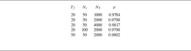
2.3. Mesh convergence
A parameter sensitivity analysis for the case $(\beta , KC, k) = (10^6, 0.185, 886)$
was conducted to evaluate the influence of
$(\beta , KC, k) = (10^6, 0.185, 886)$
was conducted to evaluate the influence of $T_f$
,
$T_f$
, $N_s$
and
$N_s$
and $N_T$
on Floquet exponent
$N_T$
on Floquet exponent $\mu$
, where
$\mu$
, where $k\ (= 2\pi /\lambda )$
is the wavenumber,
$k\ (= 2\pi /\lambda )$
is the wavenumber, $T_f$
is the period of the base flow for Floquet analysis,
$T_f$
is the period of the base flow for Floquet analysis, $N_s$
is the number of time slices used by the Floquet solver to reconstruct the base flow within one period and
$N_s$
is the number of time slices used by the Floquet solver to reconstruct the base flow within one period and $N_T$
is the number of time integration steps within one period. The results shown in table 1 demonstrated that the Floquet exponent
$N_T$
is the number of time integration steps within one period. The results shown in table 1 demonstrated that the Floquet exponent $\mu$
varied by less than
$\mu$
varied by less than $1\,\%$
under different
$1\,\%$
under different $T_f$
,
$T_f$
, $N_s$
and
$N_s$
and $N_T$
. Therefore, all simulations in this study were performed with
$N_T$
. Therefore, all simulations in this study were performed with $(T_f, N_s, N_T) = (20, 50, 2000)$
.
$(T_f, N_s, N_T) = (20, 50, 2000)$
.
The influence of $T_f$
,
$T_f$
, $N_s$
and
$N_s$
and $N_T$
on the Floquet exponent
$N_T$
on the Floquet exponent $\mu$
at
$\mu$
at $(\beta , KC, k) = (10^6, 0.185, 886)$
.
$(\beta , KC, k) = (10^6, 0.185, 886)$
.

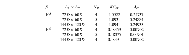
For $\beta = 10^3$
and
$\beta = 10^3$
and $10^6$
, a mesh convergence analysis of the
$10^6$
, a mesh convergence analysis of the $\textit{KC}_{cr}$
and
$\textit{KC}_{cr}$
and $\lambda _{cr}$
values obtained from Floquet analysis was conducted by varying either the polynomial order or the domain size. As evidenced in table 2, the
$\lambda _{cr}$
values obtained from Floquet analysis was conducted by varying either the polynomial order or the domain size. As evidenced in table 2, the $\textit{KC}_{cr}$
and
$\textit{KC}_{cr}$
and $\lambda _{cr}$
values varied by less than
$\lambda _{cr}$
values varied by less than $1\,\%$
when the polynomial order increased from
$1\,\%$
when the polynomial order increased from $N_p = 4$
to 5 and when the domain size increased from
$N_p = 4$
to 5 and when the domain size increased from $72D\times 60D$
to
$72D\times 60D$
to $144D\times 120D$
. Therefore,
$144D\times 120D$
. Therefore, $N_p = 4$
and
$N_p = 4$
and $L_x\times L_y = 72D\times 60D$
were adopted for the present Floquet analysis.
$L_x\times L_y = 72D\times 60D$
were adopted for the present Floquet analysis.
The influence of $N_p$
and domain size on
$N_p$
and domain size on $\textit{KC}_{cr}$
and
$\textit{KC}_{cr}$
and $\lambda _{cr}$
in Floquet analysis.
$\lambda _{cr}$
in Floquet analysis.

In 3-D DNS, the time histories of streamwise vorticity at vortex core displayed exponential growth for $\textit{KC} \gt \textit{KC}_{cr}$
and exponential decay for
$\textit{KC} \gt \textit{KC}_{cr}$
and exponential decay for $\textit{KC} \lt \textit{KC}_{cr}$
. The growth/decay rates varied linearly close to
$\textit{KC} \lt \textit{KC}_{cr}$
. The growth/decay rates varied linearly close to $\textit{KC}_{cr}$
, such that the
$\textit{KC}_{cr}$
, such that the $\textit{KC}_{cr}$
value could also be determined from DNS by identifying the zero-growth condition. For
$\textit{KC}_{cr}$
value could also be determined from DNS by identifying the zero-growth condition. For $\beta = 10^3$
and
$\beta = 10^3$
and $10^6$
, the
$10^6$
, the $\textit{KC}_{cr}$
values determined from DNS showed less than
$\textit{KC}_{cr}$
values determined from DNS showed less than $1\,\%$
variation with mesh refinement (
$1\,\%$
variation with mesh refinement ( $N_p$
from 4 to 5), halved time step (doubling the number of time steps per period from 2000 to 4000), doubled
$N_p$
from 4 to 5), halved time step (doubling the number of time steps per period from 2000 to 4000), doubled $L_z$
(from
$L_z$
(from $3\lambda _{cr}$
to
$3\lambda _{cr}$
to $6\lambda _{cr}$
) or doubled
$6\lambda _{cr}$
) or doubled $L_x\times L_y$
(from
$L_x\times L_y$
(from $72D\times 60D$
to
$72D\times 60D$
to $144D\times 120D$
). The
$144D\times 120D$
). The $\textit{KC}_{cr}$
values determined from DNS agreed well with Floquet analysis (within less than
$\textit{KC}_{cr}$
values determined from DNS agreed well with Floquet analysis (within less than $2\,\%$
error) for several values of
$2\,\%$
error) for several values of $\beta$
(
$\beta$
( $= 55,\ 80,\ 10^3,\ 10^4,\ 10^5 \text{ and } 10^6$
) tested in this study.
$= 55,\ 80,\ 10^3,\ 10^4,\ 10^5 \text{ and } 10^6$
) tested in this study.
3. Results and discussion
3.1. Determination of
$\textit{KC}_{cr}$
based on Floquet analysis

First, Floquet analysis was used to determine the $\textit{KC}_{cr}$
values for the 3-D/Honji instability over
$\textit{KC}_{cr}$
values for the 3-D/Honji instability over $\beta = 52$
–
$\beta = 52$
– $10^{6}$
. As shown in figure 5(a), the present Floquet analysis results agreed well with
$10^{6}$
. As shown in figure 5(a), the present Floquet analysis results agreed well with $\textit{KC}_{cr}$
obtained from the experiments by Honji (Reference Honji1981), Sarpkaya (Reference Sarpkaya1986) and Tatsuno & Bearman (Reference Tatsuno and Bearman1990) and, notably, were in excellent agreement with the Floquet analysis by Elston et al. (Reference Elston, Blackburn and Sheridan2006) at
$\textit{KC}_{cr}$
obtained from the experiments by Honji (Reference Honji1981), Sarpkaya (Reference Sarpkaya1986) and Tatsuno & Bearman (Reference Tatsuno and Bearman1990) and, notably, were in excellent agreement with the Floquet analysis by Elston et al. (Reference Elston, Blackburn and Sheridan2006) at $\beta = 52$
–
$\beta = 52$
– $100$
. The present
$100$
. The present $\textit{KC}_{cr}$
values also demonstrated asymptotic convergence towards the theoretical
$\textit{KC}_{cr}$
values also demonstrated asymptotic convergence towards the theoretical $\textit{KC}_{H}$
with increasing
$\textit{KC}_{H}$
with increasing $\beta$
. Specifically, for
$\beta$
. Specifically, for $\beta = 10^{2}$
,
$\beta = 10^{2}$
, $10^{3}$
,
$10^{3}$
, $10^{4}$
,
$10^{4}$
, $10^{5}$
and
$10^{5}$
and $10^{6}$
, the discrepancies were 18.17 %, 2.52 %, 0.90 %, 0.23 % and 0.17 %, respectively, which suggested that the
$10^{6}$
, the discrepancies were 18.17 %, 2.52 %, 0.90 %, 0.23 % and 0.17 %, respectively, which suggested that the $\textit{KC}_{H}$
line performs well at
$\textit{KC}_{H}$
line performs well at $\beta \gtrsim 10^{4}$
. Based on the present results, a new equation for
$\beta \gtrsim 10^{4}$
. Based on the present results, a new equation for $\textit{KC}_{cr}$
is proposed (the blue line in figure 5, where the maximum fitting error is below 1 %):
$\textit{KC}_{cr}$
is proposed (the blue line in figure 5, where the maximum fitting error is below 1 %):
 \begin{align} \textit{KC}_{cr} = \begin{cases} 20\exp (-0.0606\beta )\! +\! 1.76\exp (-0.0075\beta )\! +\! 1.45\exp (-0.00027\beta )\!\! & \!\!55\! \leq\! \beta \leq 700 \\ (5.778 + F_{1}(\beta ))\beta ^{-1/4}(1 + 0.205\beta ^{-1/4}) & \beta \geq 700, \end{cases}\end{align}
 \begin{align} F_{1}(\beta ) = 2\beta ^{-2/5}.\end{align}
The term $F_{1}(\beta )$
is introduced as a correction to the
$F_{1}(\beta )$
is introduced as a correction to the $\textit{KC}_{H}$
value calculated by (1.1). For
$\textit{KC}_{H}$
value calculated by (1.1). For $\beta \gt 10^{4}$
, the deviation between the theoretical prediction by Hall (Reference Hall1984) and the present Floquet analysis becomes less than
$\beta \gt 10^{4}$
, the deviation between the theoretical prediction by Hall (Reference Hall1984) and the present Floquet analysis becomes less than $0.5\,\%$
and (3.1) converges towards (1.1). In contrast, the
$0.5\,\%$
and (3.1) converges towards (1.1). In contrast, the $\textit{KC}_{S}$
line remains significantly lower than the present
$\textit{KC}_{S}$
line remains significantly lower than the present $\textit{KC}_{cr}$
values, the physical cause of which is explored in § 3.2.
$\textit{KC}_{cr}$
values, the physical cause of which is explored in § 3.2.
Comparison of critical stability boundaries in the $(KC, \beta )$
parameter space between present and previous studies: (a)
$(KC, \beta )$
parameter space between present and previous studies: (a) $\beta = 0$
–
$\beta = 0$
– $700$
and (b)
$700$
and (b) $\beta = 700$
–
$\beta = 700$
– $10^{7}$
.
$10^{7}$
.

3.2. Physical mechanism of the QCS
In the region of $\textit{KC}_{S} \lt \textit{KC} \lt \textit{KC}_{H}$
and
$\textit{KC}_{S} \lt \textit{KC} \lt \textit{KC}_{H}$
and $\beta = 10^{3}$
–
$\beta = 10^{3}$
– $1.4\times 10^{6}$
, Sarpkaya (Reference Sarpkaya2002) observed QCS experimentally, where the Honji vortices became pronounced near peak flow velocities but diminished during deceleration. However, other experimental and numerical studies, such as those by Honji (Reference Honji1981), Tatsuno & Bearman (Reference Tatsuno and Bearman1990), Elston et al. (Reference Elston, Blackburn and Sheridan2006) and An et al. (Reference An, Cheng and Zhao2011), all reported purely 2-D flow at
$1.4\times 10^{6}$
, Sarpkaya (Reference Sarpkaya2002) observed QCS experimentally, where the Honji vortices became pronounced near peak flow velocities but diminished during deceleration. However, other experimental and numerical studies, such as those by Honji (Reference Honji1981), Tatsuno & Bearman (Reference Tatsuno and Bearman1990), Elston et al. (Reference Elston, Blackburn and Sheridan2006) and An et al. (Reference An, Cheng and Zhao2011), all reported purely 2-D flow at $\textit{KC} \lt \textit{KC}_{H}$
, but the
$\textit{KC} \lt \textit{KC}_{H}$
, but the $\beta$
values examined in those studies were less than 700. To check whether the QCS would develop at
$\beta$
values examined in those studies were less than 700. To check whether the QCS would develop at $\beta \gt 700$
, we performed Floquet analysis and 3-D DNS at
$\beta \gt 700$
, we performed Floquet analysis and 3-D DNS at $\beta = 10^{3}$
,
$\beta = 10^{3}$
, $10^{4}$
,
$10^{4}$
, $10^{5}$
and
$10^{5}$
and $10^{6}$
and observed exponential decay of three-dimensionality of the flow at
$10^{6}$
and observed exponential decay of three-dimensionality of the flow at $\textit{KC} \lt \textit{KC}_{H}$
, which confirmed that the wake was purely 2-D regardless of the
$\textit{KC} \lt \textit{KC}_{H}$
, which confirmed that the wake was purely 2-D regardless of the $\beta$
value.
$\beta$
value.
Subsequently, 3-D DNS results were used to closely re-examine the existence or absence of the QCS. Figure 6 presents the spatiotemporal evolution of $\omega _{x}$
at phase
$\omega _{x}$
at phase $\theta = 0$
over multiple oscillation periods for
$\theta = 0$
over multiple oscillation periods for $\beta = 10^{6}$
and
$\beta = 10^{6}$
and $\textit{KC} = 0.182$
–
$\textit{KC} = 0.182$
– $0.2$
. Vorticity component
$0.2$
. Vorticity component $\omega _{x}$
was measured along the line
$\omega _{x}$
was measured along the line $x = 0$
and
$x = 0$
and $y/D = 0.502$
, which corresponded to the centre of the Honji vortices in the
$y/D = 0.502$
, which corresponded to the centre of the Honji vortices in the $y$
direction. For
$y$
direction. For $\textit{KC} = 0.2$
and
$\textit{KC} = 0.2$
and $0.188$
(
$0.188$
( $\gt \textit{KC}_{cr} = 0.184$
), the Honji vortices remained relatively regular up to
$\gt \textit{KC}_{cr} = 0.184$
), the Honji vortices remained relatively regular up to $t/T \sim 50$
and
$t/T \sim 50$
and $250$
, respectively, and then became chaotic (figure 6
a,b). For
$250$
, respectively, and then became chaotic (figure 6
a,b). For $\textit{KC} = 0.182$
(
$\textit{KC} = 0.182$
( $\lt \textit{KC}_{cr}$
), a weak Honji wake emerged due to initial random disturbance but gradually decayed to a 2-D state (figure 6
c), which suggested that the QCS was absent.
$\lt \textit{KC}_{cr}$
), a weak Honji wake emerged due to initial random disturbance but gradually decayed to a 2-D state (figure 6
c), which suggested that the QCS was absent.
Spatiotemporal evolution of streamwise vorticity ( $\omega _{x}$
) at
$\omega _{x}$
) at $\beta = 10^{6}$
for (a)
$\beta = 10^{6}$
for (a) $\textit{KC} = 0.2$
, (b)
$\textit{KC} = 0.2$
, (b) $\textit{KC} = 0.188$
, (c)
$\textit{KC} = 0.188$
, (c) $\textit{KC} = 0.182$
and (d)
$\textit{KC} = 0.182$
and (d) $\textit{KC} = 0.182$
, initialised with fully developed Honji vortices sampled at
$\textit{KC} = 0.182$
, initialised with fully developed Honji vortices sampled at $t/T = 43$
of the case with
$t/T = 43$
of the case with $\beta = 10^{6}$
and
$\beta = 10^{6}$
and $\textit{KC} = 0.2$
.
$\textit{KC} = 0.2$
.

The weak nonlinear stability theory of Hall (Reference Hall1984) suggested that the 3-D wake transition was subcritical at $\beta \to \infty$
. To investigate whether QCS was induced by a hysteresis effect, a DNS case initialised with fully developed Honji vortices (
$\beta \to \infty$
. To investigate whether QCS was induced by a hysteresis effect, a DNS case initialised with fully developed Honji vortices ( $\beta = 10^{6}$
,
$\beta = 10^{6}$
, $\textit{KC} = 0.2$
at
$\textit{KC} = 0.2$
at $t/T = 43$
; see figure 6
a) but governed by parameters
$t/T = 43$
; see figure 6
a) but governed by parameters $\beta = 10^{6}$
and
$\beta = 10^{6}$
and $\textit{KC} = 0.182$
was performed. As shown in figure 6(d), the Honji vortices decayed into a purely 2-D flow state, despite that
$\textit{KC} = 0.182$
was performed. As shown in figure 6(d), the Honji vortices decayed into a purely 2-D flow state, despite that $\textit{KC} = 0.182$
was well within the region of QCS (
$\textit{KC} = 0.182$
was well within the region of QCS ( $\textit{KC}_{S} = 0.05$
at
$\textit{KC}_{S} = 0.05$
at $\beta = 10^{6}$
), which suggested that the 3-D instability was supercritical, and the QCS was not induced by hysteresis.
$\beta = 10^{6}$
), which suggested that the 3-D instability was supercritical, and the QCS was not induced by hysteresis.
Considering that physical experiments on bluff-body flows inevitably contained sustained ambient disturbances (Williamson Reference Williamson1996b
; Sarpkaya Reference Sarpkaya2002), such as attachment of small air bubbles to the cylinder surface (Sarpkaya Reference Sarpkaya2002), we employed additional DNS cases with sustained disturbances and tried to reproduce the QCS observed experimentally by Sarpkaya (Reference Sarpkaya2002) at $\beta = 5221$
. To avoid direct interference of the sustained disturbances with the Honji vortices that developed on the top and bottom surfaces of the cylinder, sustained Gaussian white-noise disturbances with a standard deviation
$\beta = 5221$
. To avoid direct interference of the sustained disturbances with the Honji vortices that developed on the top and bottom surfaces of the cylinder, sustained Gaussian white-noise disturbances with a standard deviation $\sigma = 10^{-2}U$
were applied only to the front and rear surfaces of the cylinder, as sketched in figure 7(a). This choice of disturbance configuration was inspired by the observation of Sarpkaya (Reference Sarpkaya2002), who found that air bubbles attached to the cylinder wall could alter the flow structure. Since our primary goal was to elucidate the physical mechanism of the QCS, only one type of computationally implementable disturbance was used in the present study to demonstrate that the QCS was governed by external disturbance. Nevertheless, the form of disturbance in practice may not be unique.
$\sigma = 10^{-2}U$
were applied only to the front and rear surfaces of the cylinder, as sketched in figure 7(a). This choice of disturbance configuration was inspired by the observation of Sarpkaya (Reference Sarpkaya2002), who found that air bubbles attached to the cylinder wall could alter the flow structure. Since our primary goal was to elucidate the physical mechanism of the QCS, only one type of computationally implementable disturbance was used in the present study to demonstrate that the QCS was governed by external disturbance. Nevertheless, the form of disturbance in practice may not be unique.
Figure 7(b–d) presents time evolution of the QCS at $\beta = 5221$
and
$\beta = 5221$
and $\textit{KC} = 0.69$
(
$\textit{KC} = 0.69$
( $\lt \textit{KC}_{cr} = 0.71$
) over different flow phases. At low-velocity phases, the vortices were disordered (figure 7
b,d), whereas at high-velocity phases, well-defined and regularly spaced Honji vortices were observed (figure 7
c). Additionally, figures 8(a)–8(c) show the
$\lt \textit{KC}_{cr} = 0.71$
) over different flow phases. At low-velocity phases, the vortices were disordered (figure 7
b,d), whereas at high-velocity phases, well-defined and regularly spaced Honji vortices were observed (figure 7
c). Additionally, figures 8(a)–8(c) show the $\omega _{x}$
contours at
$\omega _{x}$
contours at $\theta = \unicode {x03C0}/2$
for
$\theta = \unicode {x03C0}/2$
for $\beta = 5221$
and
$\beta = 5221$
and $\textit{KC} = 0.5$
,
$\textit{KC} = 0.5$
, $0.65$
and
$0.65$
and $0.69$
(
$0.69$
( $\lt \textit{KC}_{cr} = 0.71$
), respectively. As
$\lt \textit{KC}_{cr} = 0.71$
), respectively. As $\textit{KC}$
increased towards
$\textit{KC}$
increased towards $\textit{KC}_{cr}$
, the QCS became increasingly organised and amplified. Both figures 7 and 8 show QCS features consistent with those observed experimentally by Sarpkaya (Reference Sarpkaya2002). The present DNS results in figures 6–8 demonstrated that the QCS was physically triggered by imposed disturbances.
$\textit{KC}_{cr}$
, the QCS became increasingly organised and amplified. Both figures 7 and 8 show QCS features consistent with those observed experimentally by Sarpkaya (Reference Sarpkaya2002). The present DNS results in figures 6–8 demonstrated that the QCS was physically triggered by imposed disturbances.
Streamwise vorticity ( $\omega _{x}$
) contours of QCS in the
$\omega _{x}$
) contours of QCS in the $x = 0$
plane at
$x = 0$
plane at $\beta = 5221$
and
$\beta = 5221$
and $\textit{KC} = 0.69$
for different flow phases. (a) Schematic diagram of the disturbance; (b)
$\textit{KC} = 0.69$
for different flow phases. (a) Schematic diagram of the disturbance; (b) $\theta = 0$
, (c)
$\theta = 0$
, (c) $\theta = \unicode {x03C0}/2$
and (d)
$\theta = \unicode {x03C0}/2$
and (d) $\theta = \unicode {x03C0}$
.
$\theta = \unicode {x03C0}$
.

Streamwise vorticity ( $\omega _{x}$
) contours of QCS in the
$\omega _{x}$
) contours of QCS in the $x = 0$
plane at
$x = 0$
plane at $\beta = 5221$
and
$\beta = 5221$
and $\theta = \unicode {x03C0}/2$
for different
$\theta = \unicode {x03C0}/2$
for different $\textit{KC}$
: (a)
$\textit{KC}$
: (a) $\textit{KC} = 0.5$
, (b)
$\textit{KC} = 0.5$
, (b) $\textit{KC} = 0.65$
and (c)
$\textit{KC} = 0.65$
and (c) $\textit{KC} = 0.69$
.
$\textit{KC} = 0.69$
.

Sarpkaya (Reference Sarpkaya2002) noted that ‘The difficulty of the determination of the stability line cannot be adequately emphasised. It depends not only on the parameters that can be controlled but also on those which are, to all intents and purposes, beyond the capacity of the experimenter to control (e.g. temperature gradients, residual background turbulence, very small air bubbles, higher-order harmonics of the vibrations, nonlinear interaction of various types of perturbations, just to imagine a few)’. Therefore, the experiments by Sarpkaya (Reference Sarpkaya2002), while carefully conducted, were subject to an unknown level of ambient disturbance inevitably contained in physical experiments. In this study, we further examined the influence of the level of disturbance on the QCS. Figure 9 presents the QCS under disturbances with $\sigma = 10^{-3}U$
,
$\sigma = 10^{-3}U$
, $5\times 10^{-3}U$
and
$5\times 10^{-3}U$
and $2\times 10^{-2}U$
for
$2\times 10^{-2}U$
for $\beta = 5221$
and
$\beta = 5221$
and $\textit{KC} = 0.69$
, which demonstrated that the strength of the QCS increased with increasing intensity of the disturbances. Figure 10 presents the QCS for
$\textit{KC} = 0.69$
, which demonstrated that the strength of the QCS increased with increasing intensity of the disturbances. Figure 10 presents the QCS for $\beta = 5221$
at different
$\beta = 5221$
at different $\textit{KC}$
and
$\textit{KC}$
and $\sigma$
values, which clearly illustrates that a higher noise intensity would make the QCS easier to be visualised at a lower
$\sigma$
values, which clearly illustrates that a higher noise intensity would make the QCS easier to be visualised at a lower $\textit{KC}$
. Therefore, a higher
$\textit{KC}$
. Therefore, a higher $\sigma$
would shift
$\sigma$
would shift $\textit{KC}_S$
away from
$\textit{KC}_S$
away from $\textit{KC}_{cr}$
, while a lower
$\textit{KC}_{cr}$
, while a lower $\sigma$
would shift
$\sigma$
would shift $\textit{KC}_S$
closer to
$\textit{KC}_S$
closer to $\textit{KC}_{cr}$
, and under the limiting condition of
$\textit{KC}_{cr}$
, and under the limiting condition of $\sigma = 0$
, the
$\sigma = 0$
, the $\textit{KC}_S$
value would converge to
$\textit{KC}_S$
value would converge to $\textit{KC}_{cr}$
.
$\textit{KC}_{cr}$
.
Streamwise vorticity ( $\omega _{x}$
) contours of QCS in the
$\omega _{x}$
) contours of QCS in the $x = 0$
plane at
$x = 0$
plane at $\beta = 5221$
,
$\beta = 5221$
, $\textit{KC} = 0.69$
and
$\textit{KC} = 0.69$
and $\theta = \unicode {x03C0}/2$
for different
$\theta = \unicode {x03C0}/2$
for different $\sigma$
values: (a)
$\sigma$
values: (a) $\sigma = 10^{-3}U$
, (b)
$\sigma = 10^{-3}U$
, (b) $\sigma = 5\times 10^{-3}U$
and (c)
$\sigma = 5\times 10^{-3}U$
and (c) $\sigma = 2\times 10^{-2}U$
.
$\sigma = 2\times 10^{-2}U$
.

Streamwise vorticity ( $\omega _{x}$
) contours of QCS in the
$\omega _{x}$
) contours of QCS in the $x = 0$
plane at
$x = 0$
plane at $\beta = 5221$
and
$\beta = 5221$
and $\theta = \unicode {x03C0}/2$
for different
$\theta = \unicode {x03C0}/2$
for different $\textit{KC}$
and
$\textit{KC}$
and $\sigma$
values.
$\sigma$
values.

The mechanism underlying the formation of the QCS, as identified above, may also explain why the QCS region widened with increasing $\beta$
(figure 5
b). With the increase in
$\beta$
(figure 5
b). With the increase in $\beta _{cr}$
, the critical Reynolds number
$\beta _{cr}$
, the critical Reynolds number $\textit{Re}_{cr}$
(
$\textit{Re}_{cr}$
( $= \beta _{cr} \times \textit{KC}_{cr}$
) also increased, i.e. the ratio between inertial force and viscous force increased, such that the disturbances were more likely to be amplified to result in the emergence of the QCS. As a result, the QCS region extended over a wider range of
$= \beta _{cr} \times \textit{KC}_{cr}$
) also increased, i.e. the ratio between inertial force and viscous force increased, such that the disturbances were more likely to be amplified to result in the emergence of the QCS. As a result, the QCS region extended over a wider range of $\textit{KC}$
values with increasing
$\textit{KC}$
values with increasing $\beta$
.
$\beta$
.
3.3. Determination of
$\lambda _{cr}$
based on Floquet analysis

The present Floquet analysis was also used to determine $\lambda _{cr}$
for the 3-D/Honji instability over
$\lambda _{cr}$
for the 3-D/Honji instability over $\beta = 52$
–
$\beta = 52$
– $10^{6}$
. As shown in figure 11, the present Floquet analysis results were in excellent agreement with the
$10^{6}$
. As shown in figure 11, the present Floquet analysis results were in excellent agreement with the $\lambda _{cr}$
line reported by Elston et al. (Reference Elston, Blackburn and Sheridan2006) at
$\lambda _{cr}$
line reported by Elston et al. (Reference Elston, Blackburn and Sheridan2006) at $\beta = 52$
–
$\beta = 52$
– $100$
and asymptotically approached the
$100$
and asymptotically approached the $\lambda _{H}$
line as
$\lambda _{H}$
line as $\beta$
increased. For
$\beta$
increased. For $\beta = 10^{2}$
,
$\beta = 10^{2}$
, $10^{3}$
,
$10^{3}$
, $10^{4}$
,
$10^{4}$
, $10^{5}$
and
$10^{5}$
and $10^{6}$
, the discrepancies were 31.02 %, 13.45 %, 7.31 %, 2.05 % and 0.99 %, respectively, which suggested that the
$10^{6}$
, the discrepancies were 31.02 %, 13.45 %, 7.31 %, 2.05 % and 0.99 %, respectively, which suggested that the $\lambda _{H}$
line may only be applicable at
$\lambda _{H}$
line may only be applicable at $\beta \gtrsim 10^6$
. Based on the present results, a new equation for
$\beta \gtrsim 10^6$
. Based on the present results, a new equation for $\lambda _{cr}$
is proposed (the blue line in figure 11, where the maximum fitting error is below 1 %):
$\lambda _{cr}$
is proposed (the blue line in figure 11, where the maximum fitting error is below 1 %):
 \begin{equation} \lambda _{cr}/{D} = \begin{cases} 5.4\exp (-0.048\beta ) + \exp (-0.0102\beta ) + 0.55\exp (-0.00088\beta ) & 55 \leq \beta \leq 700 \\ (6.951 + F_{2}(\beta ))\beta ^{-1/2} & \beta \geq 700, \end{cases} \end{equation}
 \begin{equation} F_{2}(\beta ) = 6.5\beta ^{-2/7}. \end{equation}
The term $F_{2}(\beta )$
is introduced as a correction to the
$F_{2}(\beta )$
is introduced as a correction to the $\lambda _{H}$
value calculated by (1.3). For
$\lambda _{H}$
value calculated by (1.3). For $\beta \gt 10^{6}$
, the deviation between the theoretical prediction by Hall (Reference Hall1984) and the present Floquet analysis becomes less than
$\beta \gt 10^{6}$
, the deviation between the theoretical prediction by Hall (Reference Hall1984) and the present Floquet analysis becomes less than $1\,\%$
and (3.3) converges towards (1.3). In contrast, the present results differed significantly from
$1\,\%$
and (3.3) converges towards (1.3). In contrast, the present results differed significantly from $\lambda _{S}$
reported by Sarpkaya (Reference Sarpkaya2002), and the physical mechanism for this discrepancy is explained below.
$\lambda _{S}$
reported by Sarpkaya (Reference Sarpkaya2002), and the physical mechanism for this discrepancy is explained below.
Comparison of previously obtained $\lambda$
values with those predicted by the present Floquet analysis. (a) Comparison at
$\lambda$
values with those predicted by the present Floquet analysis. (a) Comparison at $\beta = 0$
–700 and (b) comparison at
$\beta = 0$
–700 and (b) comparison at $\beta = 700$
–
$\beta = 700$
– $10^7$
.
$10^7$
.

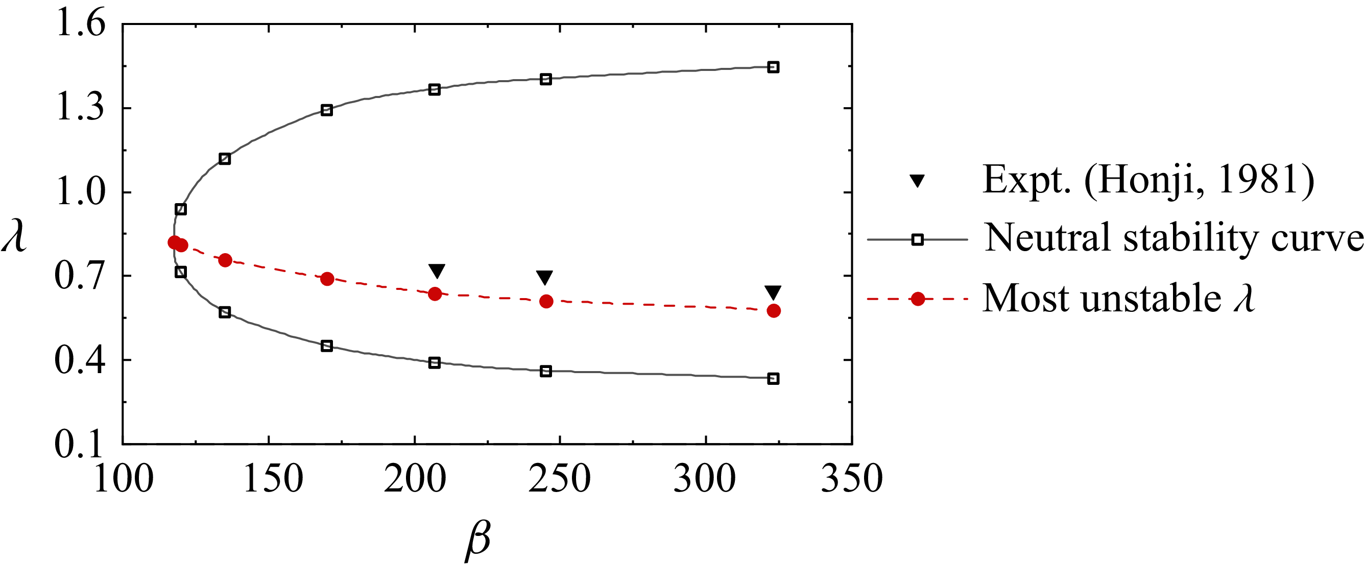
The neutral stability curve and the most unstable $\lambda$
for
$\lambda$
for $\textit{KC} = 2.14$
.
$\textit{KC} = 2.14$
.

In the region to the right of $\textit{KC}_{cr}$
(or
$\textit{KC}_{cr}$
(or $\beta _{cr}$
), we report for the first time the existence of a neutral stability curve for an oscillatory flow around a circular cylinder, which is analogous to the neutral stability curve of a circular cylinder in a unidirectional flow (Barkley & Henderson Reference Barkley and Henderson1996). For example, figure 12 shows the neutral stability curve for
$\beta _{cr}$
), we report for the first time the existence of a neutral stability curve for an oscillatory flow around a circular cylinder, which is analogous to the neutral stability curve of a circular cylinder in a unidirectional flow (Barkley & Henderson Reference Barkley and Henderson1996). For example, figure 12 shows the neutral stability curve for $\textit{KC} = 2.14$
. The critical instability at the left tip of the neutral stability curve corresponded to
$\textit{KC} = 2.14$
. The critical instability at the left tip of the neutral stability curve corresponded to $\beta _{cr} = 117.5$
and
$\beta _{cr} = 117.5$
and $\lambda _{cr} = 0.821$
. As
$\lambda _{cr} = 0.821$
. As $\beta$
increased, the Honji instability may develop over an enlarged range of
$\beta$
increased, the Honji instability may develop over an enlarged range of $\lambda$
, and the most unstable
$\lambda$
, and the most unstable $\lambda$
decreased. Physically, the most unstable
$\lambda$
decreased. Physically, the most unstable $\lambda$
corresponded to the
$\lambda$
corresponded to the $\lambda$
most likely to be observed in actual 3-D flows. This is supported by figure 12, where the most unstable
$\lambda$
most likely to be observed in actual 3-D flows. This is supported by figure 12, where the most unstable $\lambda$
predicted by the present Floquet analysis showed a trend consistent with the experimental measurements by Honji (Reference Honji1981) at
$\lambda$
predicted by the present Floquet analysis showed a trend consistent with the experimental measurements by Honji (Reference Honji1981) at $\textit{KC} = 2.14$
.
$\textit{KC} = 2.14$
.
The present finding on the strong variation of the most unstable $\lambda$
with
$\lambda$
with $\beta$
(or
$\beta$
(or $\textit{KC}$
) near the critical instability (figure 12) explains the significant discrepancy between the
$\textit{KC}$
) near the critical instability (figure 12) explains the significant discrepancy between the $\lambda _{S}$
and
$\lambda _{S}$
and $\lambda _{cr}$
lines shown in figure 11(a). The reason is that
$\lambda _{cr}$
lines shown in figure 11(a). The reason is that $\lambda _{cr}$
characterised the relationship between
$\lambda _{cr}$
characterised the relationship between $\beta$
and
$\beta$
and $\lambda$
at the critical instability (i.e. at
$\lambda$
at the critical instability (i.e. at $\textit{KC} = \textit{KC}_{cr}$
), whereas
$\textit{KC} = \textit{KC}_{cr}$
), whereas $\lambda _{S}$
established an empirical relationship using the
$\lambda _{S}$
established an empirical relationship using the $\lambda$
data over a certain region of
$\lambda$
data over a certain region of $\textit{KC}$
beyond
$\textit{KC}$
beyond $\textit{KC}_{cr}$
(open markers in figure 11
a), which may be different from the
$\textit{KC}_{cr}$
(open markers in figure 11
a), which may be different from the $\lambda _{cr}$
value at
$\lambda _{cr}$
value at $\textit{KC} = \textit{KC}_{cr}$
. Since the most unstable
$\textit{KC} = \textit{KC}_{cr}$
. Since the most unstable $\lambda$
that appeared in a 3-D flow varied with
$\lambda$
that appeared in a 3-D flow varied with $\beta$
, the
$\beta$
, the $\lambda _{S}$
value was dictated by the range of
$\lambda _{S}$
value was dictated by the range of $\beta$
used for the empirical fitting and was thus arbitrary.
$\beta$
used for the empirical fitting and was thus arbitrary.
Based on the physical understanding of the strong variation of the most unstable $\lambda$
with
$\lambda$
with $\beta$
near the critical stability, we propose an improved workflow to analyse the prior experimental data at
$\beta$
near the critical stability, we propose an improved workflow to analyse the prior experimental data at $\textit{KC} \geq \textit{KC}_{cr}$
(open markers in figure 11
a) so as to obtain improved
$\textit{KC} \geq \textit{KC}_{cr}$
(open markers in figure 11
a) so as to obtain improved $\lambda _{S}$
values (denoted
$\lambda _{S}$
values (denoted $\lambda '_{S}$
, red filled markers in figure 11
a) that better match
$\lambda '_{S}$
, red filled markers in figure 11
a) that better match $\lambda _{cr}$
. Taking
$\lambda _{cr}$
. Taking $\textit{KC} = 2.14$
as an example, (3.1) yielded
$\textit{KC} = 2.14$
as an example, (3.1) yielded $\beta _{cr} = 117.5$
for
$\beta _{cr} = 117.5$
for $\textit{KC} = 2.14$
, whereas the experimental data of
$\textit{KC} = 2.14$
, whereas the experimental data of $\lambda$
were only available at
$\lambda$
were only available at $\beta = 208$
, 245, 323 and 427 (Honji Reference Honji1981), which were far beyond
$\beta = 208$
, 245, 323 and 427 (Honji Reference Honji1981), which were far beyond $\beta _{cr}$
. Therefore, a polynomial fit was performed on the experimental results of
$\beta _{cr}$
. Therefore, a polynomial fit was performed on the experimental results of $\lambda$
for
$\lambda$
for $\textit{KC} = 2.14$
at
$\textit{KC} = 2.14$
at $\beta = 208$
–
$\beta = 208$
– $427$
, and then extrapolated to
$427$
, and then extrapolated to $\beta _{cr} = 117.5$
to obtain
$\beta _{cr} = 117.5$
to obtain $\lambda '_{S}$
. As shown in figure 11(a), the
$\lambda '_{S}$
. As shown in figure 11(a), the $\lambda '_{S}$
values significantly deviated from
$\lambda '_{S}$
values significantly deviated from $\lambda _{S}$
and demonstrated relatively good agreement with the present equation (3.3).
$\lambda _{S}$
and demonstrated relatively good agreement with the present equation (3.3).
4. Conclusions
This study addresses the long-standing discrepancies in the literature in the $\textit{KC}_{cr}$
and
$\textit{KC}_{cr}$
and $\lambda _{cr}$
values in oscillatory flow around a circular cylinder. Based on the present Floquet stability analysis and DNS results, new equations for
$\lambda _{cr}$
values in oscillatory flow around a circular cylinder. Based on the present Floquet stability analysis and DNS results, new equations for $\textit{KC}_{cr}$
and
$\textit{KC}_{cr}$
and $\lambda _{cr}$
are proposed for
$\lambda _{cr}$
are proposed for $\beta = 55$
–
$\beta = 55$
– $10^{6}$
. The present
$10^{6}$
. The present $\textit{KC}_{cr}$
and
$\textit{KC}_{cr}$
and $\lambda _{cr}$
values agree well with the numerical results of Elston et al. (Reference Elston, Blackburn and Sheridan2006) for
$\lambda _{cr}$
values agree well with the numerical results of Elston et al. (Reference Elston, Blackburn and Sheridan2006) for $\beta \sim 50$
–
$\beta \sim 50$
– $100$
and asymptotically converge to theoretical predictions by Hall (Reference Hall1984) as
$100$
and asymptotically converge to theoretical predictions by Hall (Reference Hall1984) as $\beta \to \infty$
, but deviate significantly from the empirical formulae by Sarpkaya (Reference Sarpkaya2002). The deviation between
$\beta \to \infty$
, but deviate significantly from the empirical formulae by Sarpkaya (Reference Sarpkaya2002). The deviation between $\textit{KC}_{S}$
and
$\textit{KC}_{S}$
and $\textit{KC}_{cr}$
is because
$\textit{KC}_{cr}$
is because $\textit{KC}_{S}$
corresponds to the emergence of QCS, which is physically different from the development of Honji instability. In addition, we report for the first time the existence of a neutral stability curve for an oscillatory flow around a circular cylinder, and find that the most unstable
$\textit{KC}_{S}$
corresponds to the emergence of QCS, which is physically different from the development of Honji instability. In addition, we report for the first time the existence of a neutral stability curve for an oscillatory flow around a circular cylinder, and find that the most unstable $\lambda$
varies with
$\lambda$
varies with $\beta$
(or
$\beta$
(or $\textit{KC}$
) strongly near the critical instability, such that the
$\textit{KC}$
) strongly near the critical instability, such that the $\lambda _{S}$
value is dictated by the range of
$\lambda _{S}$
value is dictated by the range of $\beta$
chosen for empirical fitting and deviates significantly from
$\beta$
chosen for empirical fitting and deviates significantly from $\lambda _{cr}$
.
$\lambda _{cr}$
.
In addition, we demonstrate that the QCS emerging below $\textit{KC}_{cr}$
is physically induced by ambient disturbances inevitably contained in physical experiments. By imposing sustained disturbances to the cylinder surface, the present DNS reproduces the QCS for the first time. The present DNS also demonstrates that the strength of the QCS increases with increasing intensity of the disturbance. Since the emergence of the QCS is governed by the intensity of sustained experimental or numerical disturbance, the
$\textit{KC}_{cr}$
is physically induced by ambient disturbances inevitably contained in physical experiments. By imposing sustained disturbances to the cylinder surface, the present DNS reproduces the QCS for the first time. The present DNS also demonstrates that the strength of the QCS increases with increasing intensity of the disturbance. Since the emergence of the QCS is governed by the intensity of sustained experimental or numerical disturbance, the $\textit{KC}_{S}$
formula by Sarpkaya (Reference Sarpkaya2002) is specific to the level of disturbance in his experimental setting and is somewhat arbitrary. Under the limiting condition of
$\textit{KC}_{S}$
formula by Sarpkaya (Reference Sarpkaya2002) is specific to the level of disturbance in his experimental setting and is somewhat arbitrary. Under the limiting condition of $\sigma = 0$
,
$\sigma = 0$
, $\textit{KC}_{S}$
would converge to
$\textit{KC}_{S}$
would converge to $\textit{KC}_{cr}$
.
$\textit{KC}_{cr}$
.
Funding
This work was supported by the National Key R&D Program of China (project ID: 2022YFB2602800) and Seed Fund of Ocean College, Zhejiang University (2025LJ003). H.J. would like to acknowledge support from the National Natural Science Foundation of China (grant no. 52301341).
Declaration of interests
The authors report no conflict of interest.


 Open access