





1. Introduction
Resolvent analysis has emerged as a powerful tool in fluid mechanics for understanding and predicting the response of fluid flows to external forcings (Schmid Reference Schmid2007; McKeon & Sharma Reference McKeon and Sharma2010). By identifying the forcing-response pairs of a dynamical system under harmonic excitation, resolvent analysis aids in uncovering the mechanisms underlying flow instabilities and interpreting turbulent dynamics. These insights are instrumental in various applications, including for example, flow control strategies, noise reduction and the design of more efficient aerodynamic systems.
The forcing and response mode pairs obtained from resolvent analysis also provide valuable information about the structural sensitivity of a flow to localised feedback mechanisms (Qadri & Schmid Reference Qadri and Schmid2017). This sensitivity analysis can be used to identify regions within the flow where small perturbations can lead to significant changes, thereby informing the optimal placement of sensors and actuators for flow control applications. Examples include controlling cavity flows (Qadri & Schmid Reference Qadri and Schmid2017) and reducing jet noise (Murthy & Bodony Reference Murthy and Bodony2024).
Despite the extensive application of resolvent analysis to various flow configurations, and the development of effective numerical techniques, including matrix-free iterative techniques (Bagheri, Brandt & Henningson Reference Bagheri, Åkervik, Brandt and Henningson2009; Monokrousos, Brandt & Henningson Reference Monokrousos, kervik, Brandt and Henningson2010; Loiseau et al. Reference Loiseau, Bucci, Cherubini and Robinet2019; Martini et al. Reference Martini, Rodríguez, Towne and Cavalieri2020), randomised numerical linear algebra methods (Liberty et al. Reference Liberty, Woolfe, Martinsson, Rokhlin and Tygert2007; Halko, Martinsson & Tropp Reference Halko, Martinsson and Tropp2011; Moarref et al. Reference Moarref, Sharma, Tropp and McKeon2013) and a recent purely data-driven approach detailed by Herrmann et al. (Reference Herrmann, Baddoo, Semaan, Brunton and McKeon2021), the extension of resolvent analysis to shock-laden flows remains insufficiently explored. Shock waves introduce discontinuities in the flow properties, leading to complexities in the linearised operators and sensitivities that are not present in smooth flows. The presence of shocks poses significant challenges in both the theoretical understanding and numerical computation of resolvent modes. Notably, there is a lack of analytical solutions against which numerically computed resolvents in shock-laden flows can be verified.
It has long been recognised that an inviscid linearisation of a shock wave is ill-posed unless the Rankine–Hugoniot jump conditions are imposed as an internal boundary: without them, the spectrum becomes pathological, admitting continuous branches and unbounded growth (Guderley Reference Guderley1942; D’yakov Reference D’yakov1954). Viscous regularisation remedies this behaviour and restores a discrete, well-posed operator, as established in classical shock-stability studies (Mack Reference Mack1984; Fedorov Reference Fedorov2011). The present work builds upon their contributions by supplying the first semi-analytic resolvent benchmark that embeds the Rankine–Hugoniot conditions and viscous effects, enabling quantitative verification of fully numerical resolvent solvers in shock-laden flows.
Additionally, prior studies have addressed related issues in the context of adjoint solutions in inviscid flows with shocks. In addition to their relevance for adjoint-based analyses, shock waves play a crucial role in transonic aerodynamic optimisation, which has become a topic of growing interest. Adjoint methods have proven particularly effective for managing shocks, as they enable the efficient computation of sensitivity gradients for performance metrics with respect to design changes (Li et al. Reference Li, Luo, Liu, Zheng and Han2024). Furthermore, aerodynamic shape optimisation remains a central strategy in shock management. Studies have shown that refining wing configurations in supersonic aircraft, through adjustments to parameters such as leading-edge sweep angles and aspect ratios, effectively delays shock wave onset and mitigates drag penalties (Reuther et al. Reference Reuther, Alonso, Rimlinger and Jameson1999). Giles et al. (Reference Giles, Pierce, Giles and Pierce1997) and Giles & Pierce (Reference Giles and Pierce2000, Reference Giles and Pierce2001) examined the properties of adjoint solutions in such flows, highlighting the need for careful treatment of discontinuities. More recently, Bodony & Fikl (Reference Bodony and Fikl2022) investigated the numerical implications of adjoint methods in the presence of shocks, emphasising the importance of using appropriate numerical schemes to achieve convergence. Collectively, these developments underscore the critical importance of addressing shock phenomena in aerodynamic optimisation, paving the way for the design of highly efficient and high-performance aerodynamic systems.
Motivated by these challenges, the present study aims to investigate the impact of flow discontinuities on the forcing-response dynamics of simple shock-laden flows. Specifically, we focus on developing semi-analytic resolvent solutions for the quasi-one-dimensional Euler and Navier–Stokes equations governing flow in a converging–diverging nozzle of arbitrary shape. By using a Green’s function approach, we construct both inviscid and viscous Green’s function operators corresponding to the forward and adjoint operators. These operators incorporate extensions that allow shocks to be included explicitly in the problem formulation.
The objectives of this study are threefold.
-
(i) Derive semi-analytic resolvent solutions for isentropic (subsonic and supersonic) and transonic flows with shocks, providing a benchmark for verifying numerical resolvent analyses in shock-laden flows.
-
(ii) Analyse the sensitivity of the resolvent solutions to disturbances across flow discontinuities, elucidating the impact of shocks on the forcing-response dynamics.
-
(iii) Assess the validity of numerical schemes used for computing adjoint and resolvent solutions in the presence of shocks, particularly those recommended by Bodony & Fikl (Reference Bodony and Fikl2022).
Our presentation is structured as follows. We begin with an introduction to resolvent analysis in § 2, and then introduce the inviscid problem in § 3, deriving the forward and adjoint Green’s function operators, and constructing the zero-frequency resolvent operator. Next, we extend the analysis to viscous shock-laden flows in § 4, highlighting the role of viscosity in resolving discrepancies between numerical and semi-analytic resolvent solutions. In § 5, we introduce a modified WENO formulation tailored for resolvent mode analysis of viscous shock-laden flows, wherein the nonlinear smoothness-based weighting is disabled during mode computations to recover a consistent linear operator and achieve close agreement with semi-analytic viscous modes while retaining WENO’s shock-capturing capabilities for the underlying flow solution. Finally, conclusions are drawn in § 6, where we discuss the implications of our findings and suggest directions for future research.
2. Resolvent analysis
Resolvent analysis identifies the most responsive forcings and most receptive responses of a dynamical system under constant-frequency excitation. Consider the system of nonlinear partial differential equations describing the compressible, viscous flow within a given computational domain. The discretised flow governing equations may be written as
 \begin{equation} \frac {\mathrm{d} \boldsymbol{Q}}{\mathrm{d} t} = \unicode{x1D649} (\boldsymbol{Q}), \end{equation}
where $\boldsymbol{Q}$
is the flow solution and
$\boldsymbol{Q}$
is the flow solution and $\unicode{x1D649}$
is the discrete nonlinear differential operator. Linearisation of (2.1) for small perturbations
$\unicode{x1D649}$
is the discrete nonlinear differential operator. Linearisation of (2.1) for small perturbations $\boldsymbol{Q}' = \boldsymbol{Q} - \bar {\boldsymbol{Q}}$
to the base-flow
$\boldsymbol{Q}' = \boldsymbol{Q} - \bar {\boldsymbol{Q}}$
to the base-flow $\bar {\boldsymbol{Q}}$
satisfying
$\bar {\boldsymbol{Q}}$
satisfying $\unicode{x1D649} (\bar {\boldsymbol{Q}}) = 0$
yields
$\unicode{x1D649} (\bar {\boldsymbol{Q}}) = 0$
yields
 \begin{equation} \frac {\mathrm{d} \boldsymbol{Q}'}{\mathrm{d} t} = \unicode{x1D647} (\bar {\boldsymbol{Q}}) \boldsymbol{Q}', \end{equation}
where $\unicode{x1D647}$
is the corresponding discrete linearised differential operator evaluated about the base-flow
$\unicode{x1D647}$
is the corresponding discrete linearised differential operator evaluated about the base-flow $\bar {\boldsymbol{Q}}$
. Next, identification of the most responsive forcings and receptive responses of the dynamical system (2.2), requires the following modifications be considered:
$\bar {\boldsymbol{Q}}$
. Next, identification of the most responsive forcings and receptive responses of the dynamical system (2.2), requires the following modifications be considered:
 \begin{align} \frac {\mathrm{d}\boldsymbol{Q}'}{\mathrm{d}t} = \unicode{x1D647} (\bar {\boldsymbol{Q}}) \boldsymbol{Q}' + \unicode{x1D63D} \boldsymbol{f}, \quad \boldsymbol{r} = \unicode{x1D63E} \boldsymbol{Q}', \end{align}
where the vector $\boldsymbol{f}$
contains zero-mean source terms of the continuity, momentum and energy equations, and represents an external forcing on the linearised, governing equations. The vector
$\boldsymbol{f}$
contains zero-mean source terms of the continuity, momentum and energy equations, and represents an external forcing on the linearised, governing equations. The vector $\boldsymbol{r}$
represents the system’s response, and the matrices
$\boldsymbol{r}$
represents the system’s response, and the matrices $\unicode{x1D63D}$
and
$\unicode{x1D63D}$
and $\unicode{x1D63E}$
specify the inputs to and outputs from the system. Next, a Fourier-transformation of the previous equations, in the form
$\unicode{x1D63E}$
specify the inputs to and outputs from the system. Next, a Fourier-transformation of the previous equations, in the form
 \begin{equation} \boldsymbol{Q}' (\boldsymbol{x},t) = \int _{-\infty }^{\infty } \boldsymbol{\hat {Q}} (\boldsymbol{x},\omega ) \textit{e}^{i \omega t} \,{\rm d} \omega , \end{equation}
yields a frequency domain system
 \begin{equation} \boldsymbol{\hat {r}} = \unicode{x1D63E} \boldsymbol{\hat {Q}} = \unicode{x1D63E} (i\omega \unicode{x1D644} - \unicode{x1D647})^{\,-1} \unicode{x1D63D} \boldsymbol{\hat {f}} = \unicode{x1D63E} \unicode{x1D64D}(\omega ) \unicode{x1D63D} \boldsymbol{\hat {f}} = \unicode{x1D643}(\omega ) \boldsymbol{\hat {f}}, \end{equation}
where $\unicode{x1D64D}(\omega )$
is the resolvent operator (Schmid Reference Schmid2007) and
$\unicode{x1D64D}(\omega )$
is the resolvent operator (Schmid Reference Schmid2007) and $\unicode{x1D643}(\omega )$
is the frequency domain input–output operator relating the forcing (
$\unicode{x1D643}(\omega )$
is the frequency domain input–output operator relating the forcing ( $\boldsymbol{\hat {f}}$
) and response (
$\boldsymbol{\hat {f}}$
) and response ( $\boldsymbol{\hat {r}}$
) modes. Next, a measure of the forcing and response mode energy is established through the introduction of positive definite norms
$\boldsymbol{\hat {r}}$
) modes. Next, a measure of the forcing and response mode energy is established through the introduction of positive definite norms $\unicode{x1D63F}_{\boldsymbol{r}}\gt 0$
and
$\unicode{x1D63F}_{\boldsymbol{r}}\gt 0$
and $\unicode{x1D63F}_{\!\boldsymbol{f}}\gt 0$
, respectively. These are usually characterised by an inner product encompassing a weighted integral over the entire domain;
$\unicode{x1D63F}_{\!\boldsymbol{f}}\gt 0$
, respectively. These are usually characterised by an inner product encompassing a weighted integral over the entire domain; $\langle \boldsymbol{a}, \boldsymbol{b} \rangle _{\boldsymbol{r}} = \boldsymbol{a}^H \unicode{x1D63F}_{\boldsymbol{r}} \boldsymbol{b} = \boldsymbol{a}^H \unicode{x1D649}^H_{\boldsymbol{r}} \unicode{x1D649}_{\boldsymbol{r}} \boldsymbol{b}$
and
$\langle \boldsymbol{a}, \boldsymbol{b} \rangle _{\boldsymbol{r}} = \boldsymbol{a}^H \unicode{x1D63F}_{\boldsymbol{r}} \boldsymbol{b} = \boldsymbol{a}^H \unicode{x1D649}^H_{\boldsymbol{r}} \unicode{x1D649}_{\boldsymbol{r}} \boldsymbol{b}$
and $\langle \boldsymbol{a}, \boldsymbol{b} \rangle _{\!\boldsymbol{f}} = \boldsymbol{a}^H \unicode{x1D63F}_{\!\boldsymbol{f}} \boldsymbol{b} = \boldsymbol{a}^H \unicode{x1D649}^H_{\!\boldsymbol{f}} \unicode{x1D649}_{\!\boldsymbol{f}} \boldsymbol{b}$
, where
$\langle \boldsymbol{a}, \boldsymbol{b} \rangle _{\!\boldsymbol{f}} = \boldsymbol{a}^H \unicode{x1D63F}_{\!\boldsymbol{f}} \boldsymbol{b} = \boldsymbol{a}^H \unicode{x1D649}^H_{\!\boldsymbol{f}} \unicode{x1D649}_{\!\boldsymbol{f}} \boldsymbol{b}$
, where $\unicode{x1D649}_{\boldsymbol{r}}$
and
$\unicode{x1D649}_{\boldsymbol{r}}$
and $\unicode{x1D649}_{\!\boldsymbol{f}}$
represent the Cholesky decomposition factors of the matrices
$\unicode{x1D649}_{\!\boldsymbol{f}}$
represent the Cholesky decomposition factors of the matrices $\unicode{x1D63F}_{\boldsymbol{r}}$
and
$\unicode{x1D63F}_{\boldsymbol{r}}$
and $\unicode{x1D63F}_{\!\boldsymbol{f}}$
, respectively. From these, the definition of a gain
$\unicode{x1D63F}_{\!\boldsymbol{f}}$
, respectively. From these, the definition of a gain $\sigma (\omega )$
, which represents the energy of the response corresponding to a unit energy forcing, follows as
$\sigma (\omega )$
, which represents the energy of the response corresponding to a unit energy forcing, follows as
 \begin{equation} \sigma ^2(\omega ) = \underset {\boldsymbol{\hat {f}}}{\text{max}} \frac {\langle \boldsymbol{\hat {r}}, \boldsymbol{\hat {r}} \rangle _{\boldsymbol{r}}}{\langle \boldsymbol{\hat {f}}, \boldsymbol{\hat {f}} \rangle _{\!\boldsymbol{f}}} = \text{max} \ \texttt {svd}\left (\unicode{x1D649}_r \unicode{x1D643}(\omega ) \unicode{x1D649}^{\,-1}_f\right )\!. \end{equation}
As mentioned in (2.6), a singular value decomposition that incorporates the forcing and response norms, and the operator $\unicode{x1D643}(\omega )$
, is then used to compute a set of optimal forcing and response modes. These modes may represent a low-ranked approximation of the forcing-response dynamics of the full system. Additionally, the forcing and response mode pairs are capable of providing the structural sensitivity of a system, such as to localised feedback in the flow. By considering perturbations
$\unicode{x1D643}(\omega )$
, is then used to compute a set of optimal forcing and response modes. These modes may represent a low-ranked approximation of the forcing-response dynamics of the full system. Additionally, the forcing and response mode pairs are capable of providing the structural sensitivity of a system, such as to localised feedback in the flow. By considering perturbations $\mathrm{d} \unicode{x1D647}$
(in the linear limit) to the operator
$\mathrm{d} \unicode{x1D647}$
(in the linear limit) to the operator $\unicode{x1D647}$
, the change in gain
$\unicode{x1D647}$
, the change in gain $\mathrm{d} \sigma$
(see Appendix D for derivation) can be evaluated as
$\mathrm{d} \sigma$
(see Appendix D for derivation) can be evaluated as
 \begin{equation} \mathrm{d} \sigma = \text{Re} \big (\boldsymbol{\hat {y}}^H (\unicode{x1D649}_r \unicode{x1D63E} ( \unicode{x1D64D}(\omega ) \ \mathrm{d} \unicode{x1D647} \unicode{x1D64D}(\omega ) ) \ \unicode{x1D63D} \unicode{x1D649}_f^{\,-1}) \ \boldsymbol{\hat {w}}/(\boldsymbol{\hat {y}}^H \boldsymbol{\hat {y}})\big ), \end{equation}
where $\boldsymbol{\hat {r}} = \sigma \unicode{x1D649}_r^{\,-1} \boldsymbol{\hat {y}}$
and
$\boldsymbol{\hat {r}} = \sigma \unicode{x1D649}_r^{\,-1} \boldsymbol{\hat {y}}$
and $\boldsymbol{\hat {f}} = \unicode{x1D649}_f^{\,-1} \boldsymbol{\hat {w}}$
. These gain sensitivities can then be used to identify locations within the flow of sensor/actuator placement for flow control applications. In the next section, we begin with the inviscid problem, deriving the forward and adjoint Green’s function operators, and constructing the zero-frequency resolvent operator.
$\boldsymbol{\hat {f}} = \unicode{x1D649}_f^{\,-1} \boldsymbol{\hat {w}}$
. These gain sensitivities can then be used to identify locations within the flow of sensor/actuator placement for flow control applications. In the next section, we begin with the inviscid problem, deriving the forward and adjoint Green’s function operators, and constructing the zero-frequency resolvent operator.
3. Resolvent analysis in inviscid shock-laden flows
Building upon the foundational work of Giles et al. (Reference Giles, Pierce, Giles and Pierce1997) and Giles & Pierce (Reference Giles and Pierce2001), who derived convergent adjoint solutions for inviscid shock-laden flows, we aim to extend these methodologies to a resolvent analysis framework. In their studies, it was demonstrated that the adjoint field exhibits a logarithmic singularity at the sonic point and maintains $C^1$
continuity across shocks when linear functionals are considered. However, Bodony & Fikl (Reference Bodony and Fikl2022) highlighted that, for quadratic functionals, many commonly used shock-capturing numerical methods fail to yield convergent adjoint solutions due to the inherent discontinuities introduced by shocks.
$C^1$
continuity across shocks when linear functionals are considered. However, Bodony & Fikl (Reference Bodony and Fikl2022) highlighted that, for quadratic functionals, many commonly used shock-capturing numerical methods fail to yield convergent adjoint solutions due to the inherent discontinuities introduced by shocks.
The present work seeks to bridge this gap by developing a semi-analytical resolvent calculation that can verify the effectiveness of numerical methods in capturing meaningful linearised operators in the presence of shocks or other discontinuities. Specifically, we focus on the quasi-one-dimensional Euler equations, which, despite their simplicity, capture the essential features of shock-laden flows in converging–diverging nozzles. This choice allows for a tractable analysis while still providing valuable insights applicable to more complex, multidimensional flows.
Our approach involves employing a Green’s function methodology to derive resolvent solutions for the inviscid case. By constructing the forward and adjoint Green’s function operators, we can account for the discontinuities introduced by shocks explicitly in the formulation. This enables us to examine the properties of the resolvent operator and its associated modes in shock-laden flows and to provide benchmarks against which numerical resolvent analyses can be validated.
3.1. Inviscid quasi-one-dimensional flow equations
The steady inviscid quasi-one-dimensional (quasi-1-D) equations representing the compressible flow through a converging–diverging nozzle are given as
 \begin{equation} \boldsymbol{\mathcal{R}}(\boldsymbol{U},h) = \frac {\mathrm{d}}{\mathrm{d}x}\! \left ( \boldsymbol{F} h\right ) -\frac {\mathrm{d} h}{\mathrm{d} x} \boldsymbol{P} = \boldsymbol{0}, \end{equation}
where
 \begin{equation} \boldsymbol{U}=\begin{bmatrix} \rho \\[3pt] \rho q \\[3pt] \rho E \end{bmatrix}\!, \ \boldsymbol{F}=\begin{bmatrix} \rho q \\[3pt] \rho q^2 + p \\[3pt] \rho q H \end{bmatrix}\!, \ \boldsymbol{P}=\begin{bmatrix} 0 \\[3pt] p \\[3pt] 0 \end{bmatrix}\!. \end{equation}
Here, $\rho$
is the density,
$\rho$
is the density, $q$
is the velocity,
$q$
is the velocity, $p$
is the pressure,
$p$
is the pressure, $E$
is the total energy,
$E$
is the total energy, $H$
is the stagnation enthalpy and
$H$
is the stagnation enthalpy and $h(x)$
represents the nozzle cross-sectional area as a function of axial position
$h(x)$
represents the nozzle cross-sectional area as a function of axial position $x$
. The system is closed by the equation of state for an ideal gas
$x$
. The system is closed by the equation of state for an ideal gas
 \begin{equation} H = E + \frac {p}{\rho } = \frac {\gamma }{\gamma -1} \frac {p}{\rho } + \frac {1}{2} q^2. \end{equation}
Additionally, if the solution to the quasi-1-D equations contains a stationary discontinuity (at $x=x_s$
), the Rankine–Hugoniot jump conditions are given by
$x=x_s$
), the Rankine–Hugoniot jump conditions are given by
 \begin{equation} \mathbf{[\![} \boldsymbol{F} \mathbf{]\!]}_{x_s^-}^{x_s^+} = 0. \end{equation}
3.2. Forward Green’s function operator
To construct the Green’s function operator $\unicode{x1D642}(x,\xi )$
for the forward linearised problem, the governing equations (3.1) are linearised about a steady base-flow
$\unicode{x1D642}(x,\xi )$
for the forward linearised problem, the governing equations (3.1) are linearised about a steady base-flow ${\boldsymbol{U}}(x)$
. The linearised operator
${\boldsymbol{U}}(x)$
. The linearised operator $\unicode{x1D647}$
acting on a perturbation
$\unicode{x1D647}$
acting on a perturbation $\boldsymbol{u}(x)$
is defined as
$\boldsymbol{u}(x)$
is defined as
 \begin{equation} \unicode{x1D647} \boldsymbol{u} = \frac {\mathrm{d}}{\mathrm{d}x} \left ( h(x) \unicode{x1D63C}(x) \boldsymbol{u} \right ) - \frac {\mathrm{d}h}{\mathrm{d}x} \unicode{x1D63D}(x) \boldsymbol{u}, \end{equation}
where
 \begin{equation} \unicode{x1D63C}(x) = \frac {\partial\! \boldsymbol{F}}{\partial \boldsymbol{U}}, \quad \unicode{x1D63D}(x) = \frac {\partial \boldsymbol{P}}{\partial \boldsymbol{U}}. \end{equation}
Next, three linearly independent homogeneous solutions $\boldsymbol{\hat {u}}_{\!j}(x)$
satisfying
$\boldsymbol{\hat {u}}_{\!j}(x)$
satisfying $\unicode{x1D647} \boldsymbol{\hat {u}}_{\!j} = \boldsymbol{0}$
are constructed. These solutions represent the fundamental modes of the linearised system.
$\unicode{x1D647} \boldsymbol{\hat {u}}_{\!j} = \boldsymbol{0}$
are constructed. These solutions represent the fundamental modes of the linearised system.
To build the operator $\unicode{x1D642}(x,\xi )$
such that
$\unicode{x1D642}(x,\xi )$
such that
 \begin{equation} \boldsymbol{u}(x) = \int _D \unicode{x1D642}(x,\xi ) \; \boldsymbol{f}(\xi ) \,{\rm d} \xi , \end{equation}
where $ \unicode{x1D647} \boldsymbol{u}(x) = \boldsymbol{f}(x)$
, a set of linearly independent piecewise solutions, composed of the homogeneous solutions
$ \unicode{x1D647} \boldsymbol{u}(x) = \boldsymbol{f}(x)$
, a set of linearly independent piecewise solutions, composed of the homogeneous solutions $\boldsymbol{\hat {u}}_{\!j}$
, is sought:
$\boldsymbol{\hat {u}}_{\!j}$
, is sought:
 \begin{equation} \boldsymbol{u}_i(x,\xi ) = \begin{cases} \boldsymbol{u}_{L,i}(x) & \text{for } x \lt \xi , \\ \boldsymbol{u}_{R,i}(x) & \text{for } x \gt \xi , \end{cases} \end{equation}
where $i$
enumerates the set of linearly independent piecewise solutions
$i$
enumerates the set of linearly independent piecewise solutions $\boldsymbol{u}_i(x,\xi )$
, satisfying
$\boldsymbol{u}_i(x,\xi )$
, satisfying
 \begin{equation} \unicode{x1D647} \boldsymbol{u}_i(x,\xi ) = \boldsymbol{f}_{\!i}(\xi ) \delta (x-\xi ), \end{equation} $\boldsymbol{u}_{L,i}(x) = a_{L,i,j} \boldsymbol{\hat {u}}_{\!j}(x)$
and
$\boldsymbol{u}_{L,i}(x) = a_{L,i,j} \boldsymbol{\hat {u}}_{\!j}(x)$
and $\boldsymbol{u}_{R,i}(x) = a_{R,i,j} \boldsymbol{\hat {u}}_{\!j}(x)$
are linear combinations of the homogeneous solutions (here, summation is implied over repeated indices). The jump conditions for constants
$\boldsymbol{u}_{R,i}(x) = a_{R,i,j} \boldsymbol{\hat {u}}_{\!j}(x)$
are linear combinations of the homogeneous solutions (here, summation is implied over repeated indices). The jump conditions for constants $a_{L,i,j}$
and
$a_{L,i,j}$
and $a_{R,i,j}$
, in the solution
$a_{R,i,j}$
, in the solution $\boldsymbol{u}_i(x,\xi )$
at
$\boldsymbol{u}_i(x,\xi )$
at $x = \xi$
, are determined by integrating the linearised equation across the singularity
$x = \xi$
, are determined by integrating the linearised equation across the singularity
 \begin{equation} \int _{\xi ^-}^{\xi ^+} \unicode{x1D647} \boldsymbol{u}_i(x,\xi ) \, \mathrm{d}x = \boldsymbol{f}_{\!i}(\xi ), \end{equation}
and choosing three linearly independent source vectors $\boldsymbol{f}_{\!i}(\xi )$
; as described by Giles & Pierce (Reference Giles and Pierce2001). Then, the Green’s function operator is constructed using the vectors
$\boldsymbol{f}_{\!i}(\xi )$
; as described by Giles & Pierce (Reference Giles and Pierce2001). Then, the Green’s function operator is constructed using the vectors $\boldsymbol{u}_i(x,\xi )$
and
$\boldsymbol{u}_i(x,\xi )$
and $\boldsymbol{f}_{\!i}(\xi )$
as
$\boldsymbol{f}_{\!i}(\xi )$
as
 \begin{equation} \unicode{x1D642}(x,\xi ) = \left ( \boldsymbol{u}_1(x,\xi ) \ | \ \boldsymbol{u}_2(x,\xi ) \ | \ \boldsymbol{u}_3(x,\xi ) \right ) \ \left ( \boldsymbol{f}_1(\xi ) \ | \ \boldsymbol{f}_2(\xi ) \ | \ \boldsymbol{f}_3(\xi ) \right )^{\,-1}, \end{equation}
where vertical lines indicate the partitioning of the row vector and array into three columns. Please refer to Giles & Pierce (Reference Giles and Pierce2001) for explicit formulae.
3.3. Adjoint Green’s function operator
Similar to the construction of the forward Green’s function, the Green’s function for the adjoint problem can be constructed using three linearly independent gradient functions ( $\boldsymbol{g}_i$
) and corresponding adjoint solutions (
$\boldsymbol{g}_i$
) and corresponding adjoint solutions ( $\boldsymbol{v}_i$
) such that
$\boldsymbol{v}_i$
) such that $\unicode{x1D647}^{\dagger } \boldsymbol{v}_i(x,\eta )= \boldsymbol{g}_i(\eta ) \delta (x-\eta )$
. To accomplish this, similar to Giles & Pierce (Reference Giles and Pierce2001), we define three objective functions
$\unicode{x1D647}^{\dagger } \boldsymbol{v}_i(x,\eta )= \boldsymbol{g}_i(\eta ) \delta (x-\eta )$
. To accomplish this, similar to Giles & Pierce (Reference Giles and Pierce2001), we define three objective functions $J_i$
, as integrals of the pressure, temperature (
$J_i$
, as integrals of the pressure, temperature ( $T$
) and velocity, over the domain
$T$
) and velocity, over the domain $D$
:
$D$
:
 \begin{equation} J_1 = \int _D p(x) \, \mathrm{d}x, \quad J_2 = \int _D T(x) \, \mathrm{d}x, \quad J_3 = \int _D q(x) \, \mathrm{d}x. \end{equation}
The corresponding gradients ( $\boldsymbol{g}_i(\eta ) = \partial k_i(\eta ) / \partial \boldsymbol{U}$
;
$\boldsymbol{g}_i(\eta ) = \partial k_i(\eta ) / \partial \boldsymbol{U}$
; $\partial p /\partial \boldsymbol{U}$
,
$\partial p /\partial \boldsymbol{U}$
, $\partial T /\partial \boldsymbol{U}$
and
$\partial T /\partial \boldsymbol{U}$
and $\partial q /\partial \boldsymbol{U}$
) of the objective function integrands (
$\partial q /\partial \boldsymbol{U}$
) of the objective function integrands ( $k_i$
such that
$k_i$
such that $J_i = \int _D k_i(x)\,\mathrm{d}x$
) are then used to linearise the augmented nonlinear objective functional
$J_i = \int _D k_i(x)\,\mathrm{d}x$
) are then used to linearise the augmented nonlinear objective functional $J_{i,j}$
(similar to (2.2) of Giles & Pierce (Reference Giles and Pierce2001)) as shown as
$J_{i,j}$
(similar to (2.2) of Giles & Pierce (Reference Giles and Pierce2001)) as shown as
 \begin{align} {\rm d}\!J_{i,j} = I_{i,j}(\xi ,\eta ) &= \int _D \bigg \{ \boldsymbol{u}_{\!j}(x,\xi ) \boldsymbol{\cdot }\frac {\partial k_i(\eta )}{\partial \boldsymbol{U}} \delta (x-\eta ) \nonumber\\ &\quad - \ k_i(\eta ) \ \delta (x-\eta ) \ \delta (x-x_s^+) \ \delta _{\!j}(\xi ) \nonumber\\ &\quad + \ k_i(\eta ) \ \delta (x-\eta ) \ \delta (x-x_s^-) \ \delta _{\!j}(\xi ) \bigg \} \ \mathrm{d}x \end{align}
 \begin{align} &= \boldsymbol{u}_{\!j}(\eta ,\xi ) \boldsymbol{\cdot }\boldsymbol{g}_i(\eta ) \nonumber\\ &\quad - \ k_i(\eta ) \ \delta (\eta -x_s^+) \ \delta _{\!j}(\xi ) \nonumber \\ &\quad + \ k_i(\eta ) \ \delta (\eta -x_s^-) \ \delta _{\!j}(\xi ), \end{align}
where $\delta _{\!j}$
represents the linearised displacement of the shock location, and the indices
$\delta _{\!j}$
represents the linearised displacement of the shock location, and the indices $i$
and
$i$
and $j$
represent the choice of objective function and linearly independent piecewise solution
$j$
represent the choice of objective function and linearly independent piecewise solution $\boldsymbol{u}_{\!j}(x,\xi )$
(with associated
$\boldsymbol{u}_{\!j}(x,\xi )$
(with associated $\boldsymbol{f}_{\!j}(\xi ) \delta (x-\xi )$
; corresponding to a jump in
$\boldsymbol{f}_{\!j}(\xi ) \delta (x-\xi )$
; corresponding to a jump in $\rho u h$
,
$\rho u h$
, $H$
or
$H$
or $p_0$
) used to compute the perturbation
$p_0$
) used to compute the perturbation $I_{i,j}$
, respectively. Then, the operator
$I_{i,j}$
, respectively. Then, the operator $ ( I_{i,1}(\xi ,\eta ) \ | \ I_{i,2}(\xi ,\eta ){} | \ I_{i,3}(\xi ,\eta ) )$
, along with the adjoint form of the linearised objective function
$ ( I_{i,1}(\xi ,\eta ) \ | \ I_{i,2}(\xi ,\eta ){} | \ I_{i,3}(\xi ,\eta ) )$
, along with the adjoint form of the linearised objective function
 \begin{equation} I_{i,j}(\xi ,\eta ) = \int _D \boldsymbol{v}_i^T(x,\eta ) \boldsymbol{f}_{\!j}(\xi ) \delta (x-\xi ) \,{\rm d}x = \boldsymbol{v}_i^T(\xi ,\eta ) \boldsymbol{f}_{\!j}(\xi ), \end{equation}
is used to evaluate
 \begin{equation} \boldsymbol{v}_i^T(\xi ,\eta ) = \left ( I_{i,1}(\xi ,\eta ) \ | \ I_{i,2}(\xi ,\eta ) \ | \ I_{i,3}(\xi ,\eta ) \right ) \ \left ( \boldsymbol{f}_1(\xi ) \ | \ \boldsymbol{f}_2(\xi ) \ | \ \boldsymbol{f}_3(\xi ) \right )^{\,-1}, \end{equation}
which is used to obtain the Green’s function for the adjoint problem, as
 \begin{equation} \unicode{x1D642}^{\dagger }(x,\eta ) = \left ( \boldsymbol{v}_1(x,\eta ) \ | \ \boldsymbol{v}_2(x,\eta ) \ | \ \boldsymbol{v}_3(x,\eta ) \right ) \ \left ( \boldsymbol{g}_1(\eta ) \ | \ \boldsymbol{g}_2(\eta ) \ | \ \boldsymbol{g}_3(\eta ) \right )^{\,-1}. \end{equation}
Furthermore, the adjoint solution $\boldsymbol{v}(x)$
corresponding to any given
$\boldsymbol{v}(x)$
corresponding to any given $\boldsymbol{g}(\eta )$
is then given by
$\boldsymbol{g}(\eta )$
is then given by
 \begin{eqnarray} \boldsymbol{v}(x) &\stackrel {\mathrm{def}}{=}& \int _D \unicode{x1D642}^{\dagger }(x, \eta ) \ \boldsymbol{g}(\eta )\, \mathrm{d}\eta , \end{eqnarray}
and substituting (3.14), (3.16) and (3.17) into (3.18) (for a detailed derivation, please refer to Appendix I), we have
 \begin{eqnarray} \boldsymbol{v}(x) &=& \int _D \unicode{x1D652}^{\,-T}(x) \begin{bmatrix} \boldsymbol{u}_1(\eta ,x)^H \\[3pt] \boldsymbol{u}_2(\eta ,x)^H \\[3pt] \boldsymbol{u}_3(\eta ,x)^H \end{bmatrix} \boldsymbol{g}(\eta )\, \mathrm{d}\eta \nonumber \\ && - \ \unicode{x1D652}^{\,-T}(x) \begin{Bmatrix} \delta _1(x) \\[3pt] 0 \\[3pt] \delta _3(x) \end{Bmatrix} \big [ \big ( p \ | \ T \ | \ q \big ) \ \unicode{x1D64F}^{\,-1} \ \boldsymbol{g} \big ]_{x_s^-}^{x_s^+}, \end{eqnarray}
where $\unicode{x1D652}(x) = ( \boldsymbol{f}_1(x) \ | \ \boldsymbol{f}_2(x) \ | \ \boldsymbol{f}_3(x) )$
and
$\unicode{x1D652}(x) = ( \boldsymbol{f}_1(x) \ | \ \boldsymbol{f}_2(x) \ | \ \boldsymbol{f}_3(x) )$
and $\unicode{x1D64F}(x) = ( \boldsymbol{g}_1(x) \ | \ \boldsymbol{g}_2(x) \ | \ \boldsymbol{g}_3(x) )$
.
$\unicode{x1D64F}(x) = ( \boldsymbol{g}_1(x) \ | \ \boldsymbol{g}_2(x) \ | \ \boldsymbol{g}_3(x) )$
.
3.4. Procedure to construct the zero-frequency resolvent modes
As a first extension of Giles & Pierce (Reference Giles and Pierce2001), we consider the zero frequency resolvent modes (forcing modes $\boldsymbol{\hat {f}}$
and response modes
$\boldsymbol{\hat {f}}$
and response modes $\boldsymbol{\hat {r}}$
). These are constructed by solving for the forcing
$\boldsymbol{\hat {r}}$
). These are constructed by solving for the forcing $\boldsymbol{\hat {f}}$
that will maximise the gain
$\boldsymbol{\hat {f}}$
that will maximise the gain $\sigma$
using the Green’s function operators of the forward and adjoint problems, which were derived in the previous subsections, as follows:
$\sigma$
using the Green’s function operators of the forward and adjoint problems, which were derived in the previous subsections, as follows:
 \begin{eqnarray} \sigma ^2 &=& \underset {\boldsymbol{\hat {f}}}{\max }\left (\frac {\big \langle \boldsymbol{\hat {r}}, \boldsymbol{\hat {r}} \big \rangle }{\big \langle \boldsymbol{\hat {f}}, \boldsymbol{\hat {f}} \big \rangle } \right ) = \underset {\boldsymbol{\hat {f}}}{\max }\left (\frac {\big \langle \unicode{x1D642}\, *\, \boldsymbol{\hat {f}}, \unicode{x1D642}\, * \, \boldsymbol{\hat {f}} \big \rangle }{\big \langle \boldsymbol{\hat {f}}, \boldsymbol{\hat {f}} \big \rangle } \right ) \end{eqnarray}
 \begin{eqnarray} &=& \underset {\boldsymbol{\hat {f}}}{\max }\left (\frac {\big \langle \boldsymbol{\hat {f}} , \unicode{x1D642}^{\dagger }\, * \, \unicode{x1D642}\, * \,\boldsymbol{\hat {f}} \big \rangle }{\big \langle \boldsymbol{\hat {f}}, \boldsymbol{\hat {f}} \big \rangle } \right )\!. \end{eqnarray}
A normalised power iteration method is used to solve the eigenvalue problem
 \begin{equation} \unicode{x1D642}^{\dagger }\, * \, \unicode{x1D642}\, * \, \boldsymbol{\hat {f}} = \sigma ^2 \boldsymbol{\hat {f}}, \end{equation}
where $*$
represents the convolution operation. We chose this iterative, matrix-free approach because it computes the action of the resolvent operator and its adjoint on state vectors without requiring the explicit formation and storage of the full resolvent matrix. This makes the method computationally efficient and scalable to problems with very fine grid resolutions or higher spatial dimensions, where the memory cost of the dense resolvent operator would be prohibitive. It should be noted, however, that for problems where the discrete operator is small enough to be stored in memory, a direct computation via a singular value decomposition (SVD) would be a more robust and preferable alternative. This produces a solution to the most-amplified-forcing (
$*$
represents the convolution operation. We chose this iterative, matrix-free approach because it computes the action of the resolvent operator and its adjoint on state vectors without requiring the explicit formation and storage of the full resolvent matrix. This makes the method computationally efficient and scalable to problems with very fine grid resolutions or higher spatial dimensions, where the memory cost of the dense resolvent operator would be prohibitive. It should be noted, however, that for problems where the discrete operator is small enough to be stored in memory, a direct computation via a singular value decomposition (SVD) would be a more robust and preferable alternative. This produces a solution to the most-amplified-forcing ( $\boldsymbol{\hat {f}}$
) and most-receptive-response,
$\boldsymbol{\hat {f}}$
) and most-receptive-response,
 \begin{equation} \boldsymbol{\hat {r}}(x) = \int _D \unicode{x1D642}(x,\xi ) \boldsymbol{\hat {f}}(\xi ) \,\mathrm{d} \xi , \end{equation}
mode corresponding to the linear system $\unicode{x1D647} \boldsymbol{\hat {r}} = \boldsymbol{\hat {f}}$
. Equations (3.11), (3.17), (3.22) and (3.23) are the key results of this section whose details are now demonstrated.
$\unicode{x1D647} \boldsymbol{\hat {r}} = \boldsymbol{\hat {f}}$
. Equations (3.11), (3.17), (3.22) and (3.23) are the key results of this section whose details are now demonstrated.
3.5. Zero-frequency resolvent analysis of shock-laden quasi-1-D flow
In this section, the zero-frequency resolvent modes corresponding to steady flow through a duct of cross-section $h(x)$
governed by the quasi-one-dimensional Euler equations (3.1) are computed using the procedure described in § 3.4 and compared against the same modes computed using a finite volume method (FVM) fitted with the Jameson–Schmidt–Turkel (JST; Jameson (Reference Jameson2017)) scheme.
$h(x)$
governed by the quasi-one-dimensional Euler equations (3.1) are computed using the procedure described in § 3.4 and compared against the same modes computed using a finite volume method (FVM) fitted with the Jameson–Schmidt–Turkel (JST; Jameson (Reference Jameson2017)) scheme.
3.5.1. Inviscid base-flow solution
Three steady quasi-1-D flows through a CD nozzle – one supersonic, one subsonic and the other shock-laden – are considered. The geometric definition of the CD nozzle is given by
 \begin{equation} h(x) = 2 - \textit{e}^{- x^2 / 0.09} \ (-2 \leqslant x \leqslant 2). \end{equation}
This modification to the CD nozzle geometry, from the one used by Giles & Pierce (Reference Giles and Pierce2001), was made to ensure that the geometry is $C^2$
smooth at every point over the domain
$C^2$
smooth at every point over the domain $(-2 \leqslant x \leqslant 2)$
. In the case of the supersonic flow, the inlet is set to a non-dimensional (as per Giles & Pierce Reference Giles and Pierce2001) stagnation enthalpy
$(-2 \leqslant x \leqslant 2)$
. In the case of the supersonic flow, the inlet is set to a non-dimensional (as per Giles & Pierce Reference Giles and Pierce2001) stagnation enthalpy $H_{\textit{in}} = 4$
, stagnation pressure
$H_{\textit{in}} = 4$
, stagnation pressure $p_{0, {in}} = 2$
and Mach number
$p_{0, {in}} = 2$
and Mach number $M_{\textit{in}}=3$
. In the case of the subsonic flow, the inlet is set to the same stagnation conditions, but a different exit condition where the static pressure is
$M_{\textit{in}}=3$
. In the case of the subsonic flow, the inlet is set to the same stagnation conditions, but a different exit condition where the static pressure is $p_{\textit{out}} = 1.98$
. Finally, a flow with the same inlet conditions and the static pressure
$p_{\textit{out}} = 1.98$
. Finally, a flow with the same inlet conditions and the static pressure $p_{\textit{out}} = 1.6$
is considered. This exit boundary condition generates a steady quasi-1-D flow that features a shock in the diverging section of the CD nozzle.
$p_{\textit{out}} = 1.6$
is considered. This exit boundary condition generates a steady quasi-1-D flow that features a shock in the diverging section of the CD nozzle.
The isentropic flows are chosen to verify the derivation for the zero-frequency resolvent modes corresponding to the quasi-1-D flow through a CD nozzle, given in § 3.4, through comparison with numerical results. The shock-laden case is used to verify that a properly selected discrete numerical methodology (as shown by Lozano & Ponsin Reference Lozano and Ponsin2012) can converge to the verified zero-frequency resolvent mode solutions computed as per § 3.4, except at $x=x_s$
.
$x=x_s$
.
3.5.2. Resolvent modes of inviscid shock-free base flows
The semi-analytic zero-frequency resolvent modes corresponding to the shock-free isentropic flows are computed by solving the eigenvalue problem that results when computing the SVD of the resolvent operator, as described in § 2. Figures 1, 2, 3 and 4, show the agreement between the resolvent solution obtained as described in §§ 2 and 3.4. As expected, no particular difficulties are encountered.
Match between forcing modes computed as per Giles & Pierce (Reference Giles and Pierce2001) (solid lines) compared with a central FVM + JST based discrete (circles) implementation for supersonic isentropic flow through a CD nozzle.

Match between response modes computed as per Giles & Pierce (Reference Giles and Pierce2001) (solid lines) compared with a central FVM + JST based discrete (circles) implementation for supersonic isentropic flow through a CD nozzle.

Match between forcing modes computed as per Giles & Pierce (Reference Giles and Pierce2001) (solid lines) compared with a central FVM + JST based discrete (circles) implementation for subsonic isentropic flow through a CD nozzle.

Match between response modes computed as per Giles & Pierce (Reference Giles and Pierce2001) (solid lines) compared with a central FVM + JST based discrete (circles) implementation for subsonic isentropic flow through a CD nozzle.

3.5.3. Adjoint and forward solutions of inviscid shock-laden base flows
Building on works such as Lozano (Reference Lozano2016) and Bodony & Fikl (Reference Bodony and Fikl2022), we use an inviscid linear finite volume discretization with JST dissipation (see Appendix A for details), implemented in a cell-centred finite volume method (FVM) framework. Following Lozano & Ponsin (Reference Lozano and Ponsin2012), we modify the boundary residuals of both the forward and adjoint solvers so that the resulting discrete adjoint is simultaneously the algebraic adjoint of the discrete forward operator and a consistent discretisation of the continuous adjoint (including its boundary conditions), and the overall scheme is therefore dual consistent. The artificial dissipation terms, combining second- and fourth-order differences, are carefully constructed to ensure compatibility with both conservation laws and the adjoint system, while preserving energy stability and avoiding spurious oscillations. This dual consistency eliminates non-physical artefacts, ensures convergence of the adjoint solutions to the analytical adjoint as grid resolution increases and provides accurate treatment of internal boundaries like shocks, resulting in well-behaved and stable adjoint fields critical for sensitivity analysis and optimisation in compressible flows.
Figures 5 and 6 illustrate this by showing agreement between the numerical adjoint ( $\boldsymbol{v}$
) and forward (
$\boldsymbol{v}$
) and forward ( $\boldsymbol{u}$
) solutions, and their respective analytic counterparts. This agreement is observed pointwise across the domain, except at the shock location (
$\boldsymbol{u}$
) solutions, and their respective analytic counterparts. This agreement is observed pointwise across the domain, except at the shock location ( $x = x_s$
). The analytic solutions are derived following the methodology outlined by Giles & Pierce (Reference Giles and Pierce2001) and the Green’s function approach described in the preceding sections, tailored for shock-laden base flows, a specific gradient
$x = x_s$
). The analytic solutions are derived following the methodology outlined by Giles & Pierce (Reference Giles and Pierce2001) and the Green’s function approach described in the preceding sections, tailored for shock-laden base flows, a specific gradient $\boldsymbol{g}$
and forcing
$\boldsymbol{g}$
and forcing $\boldsymbol{f}$
.
$\boldsymbol{f}$
.
Converged adjoint mode solution (FVM + JST based implementation, represented as  ) and solution as per Giles & Pierce (Reference Giles and Pierce2001) (represented as
  ), corresponding to the transonic shock-laden flow (shock location is indicated by
  ) through a quasi-1-D flow through a CD nozzle.

Pointwise converged (except at $x=x_s$
) forward mode solution (FVM + JST based implementation represented as
$x=x_s$
) forward mode solution (FVM + JST based implementation represented as  ) and solution as per Giles & Pierce (Reference Giles and Pierce2001) (represented as
  ) corresponding to the transonic shock-laden flow (shock location is indicated by
  ) through a quasi-1-D flow through a CD nozzle.

3.5.4. Resolvent solutions of inviscid shock-laden base flows
This section investigates a significant disagreement between resolvent solutions obtained through numerical and semi-analytic approaches when shock waves are present in the base flow. Despite successfully computing pointwise (excluding the shock location) convergent adjoint and forward solutions using the numerical method outlined in § 3.5.3, and the linear operator formulation in (2.5), significant challenges arise when attempting to resolve the resolvent modes. Figures 7 and 8 reveals a clear misalignment between the leading semi-analytic and numerical resolvent modes.
Comparison between the resolvent modes computed using (3.20) (represented as  ) and using a FVM + JST based implementation (represented as
  ).
).

Comparison between the resolvent modes computed using (3.20) (represented as  ) and using a FVM + JST based implementation (represented as
  ) with increased resolution ( $\Delta x = 2/3 \ \Delta x_{{coarse}}$
, where
$\Delta x = 2/3 \ \Delta x_{{coarse}}$
, where $\Delta x_{{coarse}}$
corresponds to the uniform grid spacing in figure 7).
$\Delta x_{{coarse}}$
corresponds to the uniform grid spacing in figure 7).

To understand the origin of these discrepancies and foreshadowing the developments in § 4.1, we augmented the numerical method by solving the viscous equations, removing the JST model and directly resolving the shock (see Appendix C for details). For small enough viscosity $(\mu \leqslant 5 \times 10^{-3})$
, the direct-resolution approach successfully reproduces the converged (including the shock region) adjoint and forward solutions from the inviscid theory, as demonstrated in figures 9 and 10, respectively. However, this alternative implementation still does not fully reconcile the differences between the analytic and numerical resolvent results, as demonstrated in figure 11 for the dominant response mode.
$(\mu \leqslant 5 \times 10^{-3})$
, the direct-resolution approach successfully reproduces the converged (including the shock region) adjoint and forward solutions from the inviscid theory, as demonstrated in figures 9 and 10, respectively. However, this alternative implementation still does not fully reconcile the differences between the analytic and numerical resolvent results, as demonstrated in figure 11 for the dominant response mode.
Converged adjoint mode solution (FVM + viscous-dissipation based implementation, represented as  ) and solution as per Giles & Pierce (Reference Giles and Pierce2001) (represented as
  ), corresponding to the transonic shock-laden flow (shock location is indicated by
  ) through a quasi-1-D flow through a CD nozzle.

Pointwise converged (except at $x=x_s$
) forward mode solution (FVM + viscous-dissipation based implementation represented as
$x=x_s$
) forward mode solution (FVM + viscous-dissipation based implementation represented as  ) and solution as per Giles & Pierce (Reference Giles and Pierce2001) (represented as
  ) corresponding to the transonic shock-laden flow (shock location is indicated by
  ) through a quasi-1-D flow through a CD nozzle.

Comparison between the resolvent modes computed using (3.20) (represented as  ) and using a FVM + viscous-dissipation ( $\mu = 5 \times 10^{-3}$
) based implementation (represented as
$\mu = 5 \times 10^{-3}$
) based implementation (represented as  ).
).

We emphasise that a detailed comparison between the JST scheme and a physically viscous formulation is not the objective here. The key result is that the inviscid semi-analytical resolvent captures the system’s resolvent response only away from the shock discontinuity; it does not account for the response at the shock itself and therefore cannot deliver the complete resolvent picture for shock-laden base flows. Consistent with this interpretation, we used the $\unicode{x1D63E}$
operator from (2.3) to remove the shock from the output space – i.e. to exclude it from the norm used to measure the response and forcing modes (and hence, from the gain
$\unicode{x1D63E}$
operator from (2.3) to remove the shock from the output space – i.e. to exclude it from the norm used to measure the response and forcing modes (and hence, from the gain $\sigma$
in (2.6)). With
$\sigma$
in (2.6)). With $\unicode{x1D63E}\neq \unicode{x1D644}$
, the agreement between the viscous-numerical and inviscid–semi-analytical resolvent modes improves markedly, as shown in figure 12. This result demonstrates that once the shock contribution is excluded from the norm, the viscous-numerical and inviscid-semi-analytical answers coincide, confirming that the inviscid model accurately captures the system’s dynamics away from the shock while providing an incomplete description of the full resolvent response that includes the shock.
$\unicode{x1D63E}\neq \unicode{x1D644}$
, the agreement between the viscous-numerical and inviscid–semi-analytical resolvent modes improves markedly, as shown in figure 12. This result demonstrates that once the shock contribution is excluded from the norm, the viscous-numerical and inviscid-semi-analytical answers coincide, confirming that the inviscid model accurately captures the system’s dynamics away from the shock while providing an incomplete description of the full resolvent response that includes the shock.
Comparison between the resolvent modes computed using (3.20) (represented as  ) and using an FVM + viscous-dissipation based implementation with a mask (represented as
  ) over the spatial location of the shock (represented as
  ).
).

4. Resolvent analysis in viscous shock-laden flows
In the preceding semi-analytical analysis of inviscid shock-laden flows, the shock was treated as a discontinuity – a sudden jump in flow properties – without considering its internal structure or the possibility of forcing and responding directly at the shock location. While this approach captures some aspects of the flow’s linear dynamics, it overlooks the impact of the shock’s internal structure on the resolvent operator and the associated sensitivities.
To address this limitation, we extend the Green’s function methodology to incorporate viscous effects, allowing the shock to be modelled as a continuous, albeit thin, region with strong gradients. This viscous extension enables the semi-analytic approach to account for the finite thickness of the shock and the associated viscous dissipation, which are essential for accurately capturing the flow’s response to disturbances at and around the shock.
By incorporating viscosity, we can resolve discrepancies observed between numerical and semi-analytic resolvent solutions seen in the inviscid analyses. The viscous Green’s function operators for both the forward and adjoint problems are derived, taking into account the additional terms introduced by viscous stresses and heat conduction, and provides a more comprehensive benchmark for evaluating numerical schemes, particularly those recommended by Bodony & Fikl (Reference Bodony and Fikl2022), ensuring that they capture the correct physical behaviour in the presence of shocks.
4.1. Viscous quasi-one-dimensional flow equations
To develop the viscous extension of the Green’s function approach to resolvent mode computation, the viscous quasi-1-D equations considered in this study are
 \begin{eqnarray} \boldsymbol{\mathcal{R}}_{v\textit{iscous}}(\boldsymbol{U},h) = \frac {\mathrm{d}}{\mathrm{d} x}(h \boldsymbol{F}) + \frac {\mathrm{d}}{\mathrm{d} x}\left (h \frac {\mathrm{d}}{\mathrm{d} x}(\boldsymbol{F}_{v,1}) \right ) + \frac {\mathrm{d} h}{\mathrm{d} x} \frac {\mathrm{d}}{\mathrm{d} x}(\boldsymbol{F}_{\!v,2}) - \frac {\mathrm{d} h}{\mathrm{d} x} \boldsymbol{P} = \boldsymbol{0}, \end{eqnarray}
where $\boldsymbol{U}$
,
$\boldsymbol{U}$
, $\boldsymbol{F}$
,
$\boldsymbol{F}$
, $\boldsymbol{P}$
,
$\boldsymbol{P}$
, $H$
and
$H$
and $h(x)$
have the same definitions as in (3.2). Additionally, the viscous fluxes are defined as
$h(x)$
have the same definitions as in (3.2). Additionally, the viscous fluxes are defined as
 \begin{equation} \boldsymbol{F}_{v,1}=\begin{bmatrix} 0 \\[3pt] -\dfrac {4 \mu q}{3} \\[3pt] -\dfrac {2 \mu q^2}{3} -\dfrac {c_p \mu T}{\textit{Pr}} \end{bmatrix}\!, \quad \boldsymbol{F}_{\!v,2}=\begin{bmatrix} 0 \\[3pt] \dfrac {4 \mu q}{3} \\[3pt] 0 \end{bmatrix}\!, \end{equation}
and the terms $\mu$
,
$\mu$
, $c_p$
and
$c_p$
and $Pr$
are the dynamic viscosity, specific heat at constant pressure and the Prandtl number of the fluid.
$Pr$
are the dynamic viscosity, specific heat at constant pressure and the Prandtl number of the fluid.
4.2. Viscous linear forward operator and basis solutions
Starting with these viscous quasi-1-D nonlinear equations, the corresponding viscous linear forward problem is given by
 \begin{multline} \unicode{x1D647}_{v\textit{iscous}} \boldsymbol{u} = \frac {\mathrm{d}}{\mathrm{d} x}\left (h \frac {\partial\! \boldsymbol{F}}{\partial \boldsymbol{U}} \ \boldsymbol{u} \right ) + \frac {\mathrm{d}}{\mathrm{d} x}\left (h \frac {\mathrm{d}}{\mathrm{d} x}\left ( \frac {\partial\! \boldsymbol{F}_{v,1}}{\partial \boldsymbol{U}} \ \boldsymbol{u} \right )\right ) + \frac {\mathrm{d} h}{\mathrm{d} x} \frac {\mathrm{d}}{\mathrm{d} x} \left ( \frac {\partial\! \boldsymbol{F}_{\!v,2}}{\partial \boldsymbol{U}} \ \boldsymbol{u} \right ) - \frac {\mathrm{d} h}{\mathrm{d} x} \frac {\partial \boldsymbol{P}}{\partial \boldsymbol{U}} \boldsymbol{u}. \end{multline}
Using $\unicode{x1D647}_{v\textit{iscous}}$
, similar to Giles & Pierce (Reference Giles and Pierce2001), piece-wise homogeneous (
$\unicode{x1D647}_{v\textit{iscous}}$
, similar to Giles & Pierce (Reference Giles and Pierce2001), piece-wise homogeneous ( $\unicode{x1D647}_{v\textit{iscous}} \ \boldsymbol{\hat {u}}_i(x) = \boldsymbol{0}$
) forward solutions
$\unicode{x1D647}_{v\textit{iscous}} \ \boldsymbol{\hat {u}}_i(x) = \boldsymbol{0}$
) forward solutions $\boldsymbol{u}(x,\xi )$
that satisfy
$\boldsymbol{u}(x,\xi )$
that satisfy
 \begin{equation} \int _D \unicode{x1D647}_{v\textit{iscous}} \ \boldsymbol{u}(x,\xi )\, \mathrm{d}\xi = \int _D \delta (x-\xi ) \boldsymbol{f}(\xi )\, \mathrm{d}\xi \end{equation}
can be constructed as follows:
 \begin{eqnarray} \boldsymbol{u}(x,\xi ) &=& a \mathscr{H}\,(x-\xi ) \ \underbrace {\left (\frac {1}{h(x)} \frac {\partial \boldsymbol{U}}{\partial m} \bigg |_{H,q} + c_m(x) \ \frac {\partial \boldsymbol{U}}{\partial q} \bigg |_{m,H} \right )}_{\boldsymbol{\hat {u}}_1(x)} \nonumber \\ & & + \ b \mathscr{H}\, (x-\xi ) \ \underbrace {\left ( \frac {\partial \boldsymbol{U}}{\partial H} \bigg |_{m,q} + c_H(x) \ \frac {\partial \boldsymbol{U}}{\partial q} \bigg |_{m,H} \right )}_{\boldsymbol{\hat {u}}_2(x)} \nonumber \\ & & + \ c \mathscr{H}\,(-(x-\xi )) \ \underbrace {\left (\frac {1}{h(x)} \frac {\partial \boldsymbol{U}}{\partial m} \bigg |_{H,q} + c_q(x) \ \frac {\partial \boldsymbol{U}}{\partial q} \bigg |_{m,H} \right )}_{\boldsymbol{\hat {u}}_3(x)}, \end{eqnarray}
where $\mathscr{H}\,(x-\xi )$
is the Heaviside step function,
$\mathscr{H}\,(x-\xi )$
is the Heaviside step function, $a$
and
$a$
and $b$
represent uniform perturbations since the nonlinear quasi-1-D equations ensure that mass flux (
$b$
represent uniform perturbations since the nonlinear quasi-1-D equations ensure that mass flux ( $m h = \rho q h$
) and stagnation enthalpy (when
$m h = \rho q h$
) and stagnation enthalpy (when $Pr=3/4$
) remain constant along the CD nozzle. The unsubscripted variable
$Pr=3/4$
) remain constant along the CD nozzle. The unsubscripted variable $c$
is a uniform amplitude term and the functions
$c$
is a uniform amplitude term and the functions $c_{\{m,H,q\}}(x)$
represent the non-uniform velocity field perturbations that ensure the homogeneity equations
$c_{\{m,H,q\}}(x)$
represent the non-uniform velocity field perturbations that ensure the homogeneity equations $\unicode{x1D647}_{v\textit{iscous}} \boldsymbol{\hat {u}}_i(x) = \boldsymbol{0}$
are satisfied.
$\unicode{x1D647}_{v\textit{iscous}} \boldsymbol{\hat {u}}_i(x) = \boldsymbol{0}$
are satisfied.
4.3. Viscous linear adjoint equations and operator
The adjoint equations and operator can be derived by considering the augmented nonlinear objective function $J$
, where the adjoint solution
$J$
, where the adjoint solution $\boldsymbol{v}$
enforces the differential flow constraints,
$\boldsymbol{v}$
enforces the differential flow constraints,
 \begin{equation} J = \int _D p \ \mathrm{d}x - \int _D \boldsymbol{v}^T \boldsymbol{\cdot }\boldsymbol{\mathcal{R}}_{v\textit{iscous}} \ \mathrm{d}x. \end{equation}
Similar to Giles & Pierce (Reference Giles and Pierce2001), we choose the objective function to be the integral of pressure along the duct. Linearising this with respect to perturbations in the flow solution $\boldsymbol{u}$
gives
$\boldsymbol{u}$
gives ${\rm d}\!J = I$
as
${\rm d}\!J = I$
as
 \begin{equation} I = \int _D \left \{ \boldsymbol{v}^T \boldsymbol{\cdot }\boldsymbol{f} - \left ( \boldsymbol{v}^T \boldsymbol{\cdot }\left ( \unicode{x1D647}_{v\textit{iscous}} \ \boldsymbol{u} \right ) - \left (\frac {\partial p}{\partial \boldsymbol{U}} \right )^T \boldsymbol{\cdot }\boldsymbol{u} \ \right )\right \}\, \mathrm{d}x. \end{equation}
Integration by parts is used (see Appendix E for details) to transfer the differential operator $\unicode{x1D647}_{v\textit{iscous}}$
from
$\unicode{x1D647}_{v\textit{iscous}}$
from $\boldsymbol{u}$
to the variable
$\boldsymbol{u}$
to the variable $\boldsymbol{v}$
as shown as follows, starting with
$\boldsymbol{v}$
as shown as follows, starting with $\unicode{x1D63C} = {\partial\! \boldsymbol{F}}/{\partial \boldsymbol{U}}$
,
$\unicode{x1D63C} = {\partial\! \boldsymbol{F}}/{\partial \boldsymbol{U}}$
, $\unicode{x1D63E}_1 = {\partial\! \boldsymbol{F}_{v,1}}/{\partial \boldsymbol{U}}$
,
$\unicode{x1D63E}_1 = {\partial\! \boldsymbol{F}_{v,1}}/{\partial \boldsymbol{U}}$
, $\unicode{x1D63E}_2 = {\partial\! \boldsymbol{F}_{\!v,2}}/{\partial \boldsymbol{U}}$
,
$\unicode{x1D63E}_2 = {\partial\! \boldsymbol{F}_{\!v,2}}/{\partial \boldsymbol{U}}$
, $\unicode{x1D63D} = {\partial \boldsymbol{P}}/{\partial \boldsymbol{U}}$
and
$\unicode{x1D63D} = {\partial \boldsymbol{P}}/{\partial \boldsymbol{U}}$
and $\boldsymbol{g} = {\partial p}/{\partial \boldsymbol{U}}$
, to yield
$\boldsymbol{g} = {\partial p}/{\partial \boldsymbol{U}}$
, to yield
 \begin{eqnarray} I &=& \int _D \boldsymbol{v}^T \boldsymbol{\cdot }\boldsymbol{f} \ \mathrm{d}x - \Bigg [\boldsymbol{v}^T \boldsymbol{\cdot }\left ( h \unicode{x1D63C} \boldsymbol{u}\right ) - \boldsymbol{v}^T \boldsymbol{\cdot }\left ( h \frac {\mathrm{d}}{\mathrm{d}x} \left ( \unicode{x1D63E}_1 \boldsymbol{u} \right ) \right ) + \frac {\mathrm{d} \boldsymbol{v}^T}{\mathrm{d}x} \boldsymbol{\cdot }\left ( h \unicode{x1D63E}_1 \boldsymbol{u} \right ) \nonumber\\[3pt] && -\! \left (\frac {\mathrm{d} h}{\mathrm{d} x} \boldsymbol{v}\right )^T \boldsymbol{\cdot }\left ( \unicode{x1D63E}_2 \boldsymbol{u}\right ) \Bigg ]_{x=x_{\textit{inlet}}}^{x=x_{\textit{outlet}}} - \int _D \boldsymbol{u}^T \boldsymbol{\cdot }\bigg ( - h \unicode{x1D63C}^T \frac {\mathrm{d} \boldsymbol{v}}{\mathrm{d} x} + \unicode{x1D63E}_1^T \frac {\mathrm{d}}{\mathrm{d} x} \left ( h \frac {\mathrm{d} \boldsymbol{v}}{\mathrm{d} x} \right ) \nonumber\\[3pt] && -\! \unicode{x1D63E}_2^T \ \frac {\mathrm{d} }{\mathrm{d} x} \left ( \frac {\mathrm{d} h}{\mathrm{d} x} \boldsymbol{v} \right ) - \frac {\mathrm{d}h}{\mathrm{d}x} \ \unicode{x1D63D}^T\! \boldsymbol{v} - \ \frac {\partial p}{\partial \boldsymbol{U}} \bigg ) \ \mathrm{d}x. \end{eqnarray}
Therefore, given the boundary conditions from (4.8) and the requirement that
 \begin{equation} I = \int _D \boldsymbol{u}^T \boldsymbol{\cdot }\boldsymbol{g} \ \mathrm{d}x = \int _D \boldsymbol{v}^T \boldsymbol{\cdot }\boldsymbol{f} \ \mathrm{d}x, \end{equation}
the viscous adjoint equation, with adjoint operator $\unicode{x1D647}_{v\textit{iscous}}^{\dagger }$
and the gradient
$\unicode{x1D647}_{v\textit{iscous}}^{\dagger }$
and the gradient $\boldsymbol{g} = \partial p/\partial \boldsymbol{U}$
), is given by
$\boldsymbol{g} = \partial p/\partial \boldsymbol{U}$
), is given by
 \begin{equation} \unicode{x1D647}_{v\textit{iscous}}^{\dagger } \boldsymbol{v} - \boldsymbol{g} = - h \unicode{x1D63C}^T \frac {\mathrm{d} \boldsymbol{v}}{\mathrm{d} x} + \unicode{x1D63E}_1^T \frac {\mathrm{d}}{\mathrm{d} x} \left ( h \frac {\mathrm{d} \boldsymbol{v}}{\mathrm{d} x} \right ) - \unicode{x1D63E}_2^T \ \frac {\mathrm{d} }{\mathrm{d} x} \left ( \frac {\mathrm{d} h}{\mathrm{d} x} \boldsymbol{v} \right ) - \ \frac {\mathrm{d}h}{\mathrm{d}x} \unicode{x1D63D}^T\! \boldsymbol{v} - \frac {\partial p}{\partial \boldsymbol{U}}. \end{equation}
4.4. Viscous adjoint solutions corresponding to a specific gradient
The adjoint basis solutions can be computed by starting with (4.9), which represents the linearised objective function, the impulse forcing ( $\boldsymbol{f}(\xi ) \delta (x-\xi )$
) such that
$\boldsymbol{f}(\xi ) \delta (x-\xi )$
) such that
 \begin{equation} \unicode{x1D647}_{v\textit{iscous}} \ \boldsymbol{u}(x,\xi ) = \boldsymbol{f}(\xi ) \delta (x-\xi ) \end{equation}
and
 \begin{equation} I(\xi ) = \int _D \boldsymbol{g}^T \boldsymbol{\cdot }\boldsymbol{u}(x, \xi ) \ \mathrm{d}x - \int _D \boldsymbol{v}^T \boldsymbol{\cdot }\left ( \unicode{x1D647}_{v\textit{iscous}} \ \boldsymbol{u}(x,\xi ) - \boldsymbol{f}(\xi ) \delta (x-\xi ) \right )\, \mathrm{d}x. \end{equation}
Next, (4.12) can be transformed to a form similar to (4.8) as shown later, using another integration by parts procedure (see Appendix F for details), assuming $\unicode{x1D647}^\dagger _{v\textit{iscous}} \boldsymbol{v} - \boldsymbol{g} = \boldsymbol{0}$
and that the adjoint solutions satisfy the adjoint boundary conditions, then together with (4.11), we have
$\unicode{x1D647}^\dagger _{v\textit{iscous}} \boldsymbol{v} - \boldsymbol{g} = \boldsymbol{0}$
and that the adjoint solutions satisfy the adjoint boundary conditions, then together with (4.11), we have
 \begin{align} I(\xi ) &= \int _D \boldsymbol{v}^T\!(x) \boldsymbol{\cdot }\left \{ \unicode{x1D647}_{v\textit{iscous}} \ \boldsymbol{u}(x,\xi ) \right \} \, \mathrm{d}x \\[-12pt]\nonumber \end{align}
 \begin{align} &= \Bigg \{ \boldsymbol{v}^T (x) \boldsymbol{\cdot }\left ( h(x) \unicode{x1D63C} \boldsymbol{\hat {p}}_1(x) \right ) + \boldsymbol{v}^T (x) \boldsymbol{\cdot }\left ( h(x) \frac {\mathrm{d}}{\mathrm{d}x}\! \left ( \unicode{x1D63E}_1 \boldsymbol{\hat {p}}_1(x) \right ) \right ) \nonumber\\ &\quad + \ \boldsymbol{v}^T (x) \boldsymbol{\cdot }\left ( \frac {\mathrm{d} h(x)}{\mathrm{d} x} \unicode{x1D63E}_2 \boldsymbol{\hat {p}}_1(x) \right ) - \frac {\mathrm{d} \boldsymbol{v}^T\!(x)}{\mathrm{d}x} \boldsymbol{\cdot }\left ( h(x) \unicode{x1D63E}_1 \boldsymbol{\hat {p}}_1(x) \right ) \Bigg \} \Bigg |_{x = \xi } + \textit{BCs}, \end{align}
where the solution $\boldsymbol{u}(x,\xi )$
is assumed to have the form
$\boldsymbol{u}(x,\xi )$
is assumed to have the form $H(x-\xi ) \boldsymbol{\hat {p}}_1(x) + \boldsymbol{\hat {p}}_2(x)$
, both
$H(x-\xi ) \boldsymbol{\hat {p}}_1(x) + \boldsymbol{\hat {p}}_2(x)$
, both $\boldsymbol{\hat {p}}_{i=1,2}$
are homogeneous solutions that satisfy
$\boldsymbol{\hat {p}}_{i=1,2}$
are homogeneous solutions that satisfy $\unicode{x1D647}_{v\textit{iscous}} \boldsymbol{\hat {p}}_{i} = \boldsymbol{0}$
and
$\unicode{x1D647}_{v\textit{iscous}} \boldsymbol{\hat {p}}_{i} = \boldsymbol{0}$
and $\textit{BCs}$
are the boundary conditions that emerge as a consequence of the integration by parts procedure; see Appendix F for details. Furthermore, the boundary conditions are satisfied for all
$\textit{BCs}$
are the boundary conditions that emerge as a consequence of the integration by parts procedure; see Appendix F for details. Furthermore, the boundary conditions are satisfied for all $\xi$
(on account of the properly constructed solutions
$\xi$
(on account of the properly constructed solutions $\boldsymbol{u}(x,\xi )$
) and we have the equation
$\boldsymbol{u}(x,\xi )$
) and we have the equation
 \begin{eqnarray} I(\xi ) &=& \boldsymbol{v}^T (\xi ) \boldsymbol{\cdot }\bigg ( h(\xi ) \unicode{x1D63C} \boldsymbol{\hat {p}}_1(\xi ) + h(\xi ) \ \frac {\mathrm{d}}{\mathrm{d} \xi } \big ( \unicode{x1D63E}_1 \boldsymbol{\hat {p}}_1(\xi ) \big ) + \frac {\mathrm{d} h(\xi )}{\mathrm{d} \xi } \unicode{x1D63E}_2 \boldsymbol{\hat {p}}_1(\xi ) \bigg ) \nonumber \\ && - \frac {\mathrm{d} \boldsymbol{v}^T(\xi )}{\mathrm{d} \xi } \boldsymbol{\cdot }\big ( h(\xi ) \unicode{x1D63E}_1 \boldsymbol{\hat {p}}_1(\xi ) \big ). \end{eqnarray}
In the next section, we discuss how solutions to (4.15) are used to compute the adjoint Green’s function operator.
4.5. Viscous adjoint Green’s function operator
Starting with (4.15) from the previous section with $\boldsymbol{u}_{\!j}(x, \xi ) = \mathscr{H}\,(x-\xi ) \boldsymbol{\hat {u}}_{\!j}(x)$
and similar to (3.13), we consider the objective function perturbation
$\boldsymbol{u}_{\!j}(x, \xi ) = \mathscr{H}\,(x-\xi ) \boldsymbol{\hat {u}}_{\!j}(x)$
and similar to (3.13), we consider the objective function perturbation $I_{i,j}(\xi , \eta )$
as follows:
$I_{i,j}(\xi , \eta )$
as follows:
 \begin{eqnarray} I_{i,j}(\xi , \eta ) &=& \int _D \big \{ \boldsymbol{g}_i^T(\eta ) \ \delta (x-\eta ) \big \} \boldsymbol{\cdot }\boldsymbol{u}_{\!j}(x, \xi ) \ \mathrm{d}x \nonumber \\ &=& \boldsymbol{v}_i^T (\xi ,\eta ) \boldsymbol{\cdot }\big ( h(\xi ) \unicode{x1D63C} \boldsymbol{\hat {u}}_{\!j}(\xi ) + h(\xi ) \frac {\mathrm{d}}{\mathrm{d} \xi } \left ( \unicode{x1D63E}_1 \boldsymbol{\hat {u}}_{\!j}(\xi ) \right ) \nonumber \\ && + \frac {\mathrm{d} h(\xi )}{\mathrm{d} \xi } \ \unicode{x1D63E}_2 \boldsymbol{\hat {u}}_{\!j}(\xi ) \big ) - \frac {\partial \boldsymbol{v}_i^T(\xi ,\eta )}{\partial \xi } \boldsymbol{\cdot }\left ( h(\xi ) \unicode{x1D63E}_1 \boldsymbol{\hat {u}}_{\!j}(\xi ) \right )\!, \end{eqnarray}
such that
 \begin{eqnarray} \boldsymbol{g}_i^T(\eta ) \boldsymbol{\cdot }\boldsymbol{u}_{\!j}(\eta , \xi ) &=& \boldsymbol{v}_i^T (\xi ,\eta ) \boldsymbol{\cdot }\bigg \{ h(\xi ) \unicode{x1D63C} \boldsymbol{\hat {u}}_{\!j}(\xi ) \nonumber \\ && + h(\xi ) \ \frac {\mathrm{d}}{\mathrm{d} \xi } \left ( \unicode{x1D63E}_1 \boldsymbol{\hat {u}}_{\!j}(\xi ) \right ) + \frac {\mathrm{d} h(\xi )}{\mathrm{d} \xi } \unicode{x1D63E}_2 \boldsymbol{\hat {u}}_{\!j}(\xi ) \bigg \} \nonumber \\ && - \frac {\partial \boldsymbol{v}_i^T(\xi ,\eta )}{\partial \xi } \boldsymbol{\cdot }\left ( h(\xi ) \unicode{x1D63E}_1 \boldsymbol{\hat {u}}_{\!j}(\xi ) \right )\!. \end{eqnarray}
Upon solving (see Appendix H for details) (4.17) for $\boldsymbol{v}_i(\xi ,\eta )$
for a given gradient
$\boldsymbol{v}_i(\xi ,\eta )$
for a given gradient $\boldsymbol{g}_i(\eta )$
, the viscous adjoint Green’s function operator
$\boldsymbol{g}_i(\eta )$
, the viscous adjoint Green’s function operator $\unicode{x1D642}_{v\textit{iscous}}^{\dagger }(x,\eta )$
can be computed, by first setting the dummy variable
$\unicode{x1D642}_{v\textit{iscous}}^{\dagger }(x,\eta )$
can be computed, by first setting the dummy variable $\xi$
to
$\xi$
to $x$
for convenience, and then similar to (3.17), we have
$x$
for convenience, and then similar to (3.17), we have
 \begin{eqnarray} \unicode{x1D642}_{v\textit{iscous}}^{\dagger }(x,\eta ) &=& \left ( \boldsymbol{v}_1(x,\eta ) \ | \ \boldsymbol{v}_2(x,\eta ) \ | \ \boldsymbol{v}_3(x,\eta ) \right ) \boldsymbol{\cdot }\left ( \boldsymbol{g}_1(\eta ) \ | \ \boldsymbol{g}_2(\eta ) \ | \ \boldsymbol{g}_3(\eta ) \right )^{\,-1}. \end{eqnarray}
4.6. Viscous forward Green’s function operator
Starting with equations (4.12), (4.13), the forward solutions $\boldsymbol{\tilde {u}}_i(x,\xi )$
such that
$\boldsymbol{\tilde {u}}_i(x,\xi )$
such that
 \begin{equation} \unicode{x1D647}_{v\textit{iscous}} \boldsymbol{\tilde {u}}_i(x,\xi ) = \boldsymbol{\hat {f}}_i(\xi ) \delta (x-\xi ) \end{equation}
and the adjoint solutions $\boldsymbol{v}_{\!j}(x,\eta )$
such that
$\boldsymbol{v}_{\!j}(x,\eta )$
such that
 \begin{equation} \unicode{x1D647}^{\dagger }_{v\textit{iscous}} \boldsymbol{v}_{\!j}(x,\eta ) = \boldsymbol{g}_{\!j}(\eta ) \delta (x-\eta ), \end{equation}
and using (4.9), we have
 \begin{align} \int _D \delta (x-\eta ) \boldsymbol{g}_{\!j}^T(\eta ) \boldsymbol{\cdot }\boldsymbol{\tilde {u}}_i(x,\xi ) \,\mathrm{d}x &= \int _D \boldsymbol{v}_{\!j}^T(x,\eta ) \boldsymbol{\cdot }\boldsymbol{\hat {f}}_i(\xi ) \delta (x-\xi )\, \mathrm{d}x \\[-12pt]\nonumber \end{align}
 \begin{align} \Rightarrow \boldsymbol{\tilde {u}}_i(\eta ,\xi ) = (\boldsymbol{g}_1(\eta ),\boldsymbol{g}_2(\eta ),\boldsymbol{g}_3(\eta ))^{\,-T} &\boldsymbol{\cdot }(\boldsymbol{v}_1(\xi ,\eta ),\boldsymbol{v}_2(\xi ,\eta ),\boldsymbol{v}_3(\xi ,\eta ))^T \boldsymbol{\cdot }\boldsymbol{\hat {f}}_i(\xi ), \end{align}
and replacing the dummy variable $\eta$
with
$\eta$
with $x$
, we have
$x$
, we have
 \begin{align} \boldsymbol{\tilde {u}}_i(x,\xi ) = (\boldsymbol{g}_1(x),\boldsymbol{g}_2(x),\boldsymbol{g}_3(x))^{\,-T} \boldsymbol{\cdot }(\boldsymbol{v}_1(\xi ,x),\boldsymbol{v}_2(\xi ,x),\boldsymbol{v}_3(\xi ,x))^T \boldsymbol{\cdot }\boldsymbol{\hat {f}}_i(\xi ). \end{align}
Next, three linearly independent vectors $\boldsymbol{\hat {f}}_i$
must be computed. This can be accomplished by considering the basis vectors
$\boldsymbol{\hat {f}}_i$
must be computed. This can be accomplished by considering the basis vectors $\boldsymbol{u}_i(x,\xi )=H(x-\xi ) \boldsymbol{\hat {u}}_{i}(x)$
(with
$\boldsymbol{u}_i(x,\xi )=H(x-\xi ) \boldsymbol{\hat {u}}_{i}(x)$
(with $\unicode{x1D647}_{v\textit{iscous}} \boldsymbol{\hat {u}}_{i} = \boldsymbol{0}$
) and evaluating the following equation to compute the corresponding
$\unicode{x1D647}_{v\textit{iscous}} \boldsymbol{\hat {u}}_{i} = \boldsymbol{0}$
) and evaluating the following equation to compute the corresponding $\boldsymbol{\hat {f}}_i$
(see Appendix G for details):
$\boldsymbol{\hat {f}}_i$
(see Appendix G for details):
 \begin{eqnarray} \boldsymbol{\hat {f}}_i(x) &=& h(x) \frac {\partial\! \boldsymbol{F}}{\partial \boldsymbol{U}} \boldsymbol{\hat {u}}_{i}(x) + h(x) \frac {\mathrm{d}}{\mathrm{d} x} \left ( \frac {\partial\! \boldsymbol{F}_{v,1}}{\partial \boldsymbol{U} } \boldsymbol{\hat {u}}_{i}(x) \right ) \nonumber \\ & & + \frac {\mathrm{d}}{\mathrm{d} x} \left [ h(x)\! \left ( \frac {\partial\! \boldsymbol{F}_{v,1}}{\partial \boldsymbol{U} } \boldsymbol{\hat {u}}_{i}(x) \right ) \right ] + \frac {\mathrm{d} h}{\mathrm{d} x} \left ( \frac {\partial\! \boldsymbol{F}_{\!v,2}}{\partial \boldsymbol{U} } \boldsymbol{\hat {u}}_{i}(x) \right )\!. \end{eqnarray}
It is important to note that the equation
 \begin{equation} \int _D \unicode{x1D647}_{v\textit{iscous}} \boldsymbol{u}_i(x,\xi ) \,{\rm d}x = \int _D \boldsymbol{\hat {f}}_i(\xi ) \delta (x-\xi )\, {\rm d}x \end{equation}
is not necessarily the same as (4.19), and hence the solutions $\boldsymbol{u}_i(x,\xi )$
and
$\boldsymbol{u}_i(x,\xi )$
and $\boldsymbol{\tilde {u}}_i(x,\xi )$
can differ. Finally, the viscous forward Green’s function operator can now be constructed as follows:
$\boldsymbol{\tilde {u}}_i(x,\xi )$
can differ. Finally, the viscous forward Green’s function operator can now be constructed as follows:
 \begin{eqnarray} \unicode{x1D642}_{v\textit{iscous}}(x,\xi ) &=& (\boldsymbol{\tilde {u}}_1(x,\xi ),\boldsymbol{\tilde {u}}_2(x,\xi ),\boldsymbol{\tilde {u}}_3(x,\xi )) \boldsymbol{\cdot }(\boldsymbol{\hat {f}}_1(\xi ),\boldsymbol{\hat {f}}_2(\xi ),\boldsymbol{\hat {f}}_3(\xi ))^{\,-1}. \end{eqnarray}
4.7. Resolvent solutions corresponding to viscous shock-laden base flows
Similar to the inviscid case, the viscous ( $\mu \gt 0$
) zero-frequency resolvent modes corresponding to the shock-laden flows are computed by solving the eigenvalue problem that originates when computing the SVD of the resolvent operator
$\mu \gt 0$
) zero-frequency resolvent modes corresponding to the shock-laden flows are computed by solving the eigenvalue problem that originates when computing the SVD of the resolvent operator $\unicode{x1D64D}_{v\textit{iscous}}$
, using the numerical approach given by
$\unicode{x1D64D}_{v\textit{iscous}}$
, using the numerical approach given by
 \begin{equation} \unicode{x1D64D}_{v\textit{iscous}}^{\dagger } \ \unicode{x1D64D}_{v\textit{iscous}} \boldsymbol{f} = \sigma ^2 \boldsymbol{f} \quad \text{and} \quad \boldsymbol{r} = \unicode{x1D64D}_{v\textit{iscous}} \boldsymbol{f}, \end{equation}
converge to the modes computed using the semi-analytic Green’s function approach with the viscous extension
 \begin{equation} \unicode{x1D642}_{v\textit{iscous}}^{\dagger } * \unicode{x1D642}_{v\textit{iscous}} * \boldsymbol{f} = \sigma ^2 \boldsymbol{f} \ \ \ \ \text{and} \ \ \ \ \boldsymbol{r} =\unicode{x1D642}_{v\textit{iscous}} * \boldsymbol{f} \end{equation}
when shock-laden base-flows are considered, as shown in figures 13 and 14. Unlike classic convective instabilities where forcing and response are significantly separated, here the energy amplification is concentrated within the shock structure itself. However, this spatial overlap does not imply weak non-normality. On the contrary, the operator remains highly non-normal. The non-orthogonality of the eigenmodes arises not from large-scale spatial displacement, but from the subtle yet crucial misalignment in the modal structures. While the spatial envelopes of the forcing and response are similar, their internal phase and amplitude distributions across the different state variables are distinct. It is this structural difference that permits transient energy growth, confirming that the significant non-normality of the system is a highly localised phenomenon tied directly to the physics of the shock wave.
Numerical resolvent forcing mode solution ( ) and solution as per the viscous ( $\mu = 5 \times 10^{-3}$
) extension of Giles & Pierce (Reference Giles and Pierce2001) (
$\mu = 5 \times 10^{-3}$
) extension of Giles & Pierce (Reference Giles and Pierce2001) ( ), corresponding to the transonic shock-laden flow through a quasi-1-D model of flow through a CD nozzle.

Numerical resolvent response mode solution ( ) and solution as per the viscous ( $\mu = 5 \times 10^{-3}$
) extension of Giles & Pierce (Reference Giles and Pierce2001) (
$\mu = 5 \times 10^{-3}$
) extension of Giles & Pierce (Reference Giles and Pierce2001) ( ), corresponding to the transonic shock-laden flow through a quasi-1-D model of flow through a CD nozzle.

The steps involved in computing the semi-analytic resolvent mode solution, represented by the (4.28), are summarised as follows.
-
(i) The following two point boundary value problem is solved to compute the base-flow solution ( $q(x)$
and thus
$\boldsymbol{U}(x)$
):(4.29)where
\begin{eqnarray} \frac {\mathrm{d} \left ( \rho q^2 h + p h\right )}{\mathrm{d} x} - p \frac {\mathrm{d} h}{\mathrm{d} x} +\frac {4 \mu }{3} \left (- \frac {\mathrm{d} \left (h \dfrac {\mathrm{d} q}{\mathrm{d} x}\right )}{\mathrm{d} x} + \frac {\mathrm{d} q}{\mathrm{d} x} \frac {\mathrm{d} h}{\mathrm{d} x} \right ) = 0, \end{eqnarray}
$\rho = Q/(h q), \ e = (H - ({1}/{2}) q^2)/\gamma , \ p = (\gamma -1) \rho e,$
with boundary conditions
$ q_{x,\text{in}}= 0$
,
$q_{\textit{out}} = \{ (p_{\textit{out}}^2 h_{\textit{out}}^2 \gamma ^2)/((\gamma -1)^2 Q^2) + 2 H\}^{1/2} - (\gamma p_{\textit{out}} h_{\textit{out}})/((\gamma -1) Q)$
.
$q(x)$
and thus
$\boldsymbol{U}(x)$
):(4.29)where
\begin{eqnarray} \frac {\mathrm{d} \left ( \rho q^2 h + p h\right )}{\mathrm{d} x} - p \frac {\mathrm{d} h}{\mathrm{d} x} +\frac {4 \mu }{3} \left (- \frac {\mathrm{d} \left (h \dfrac {\mathrm{d} q}{\mathrm{d} x}\right )}{\mathrm{d} x} + \frac {\mathrm{d} q}{\mathrm{d} x} \frac {\mathrm{d} h}{\mathrm{d} x} \right ) = 0, \end{eqnarray}
$\rho = Q/(h q), \ e = (H - ({1}/{2}) q^2)/\gamma , \ p = (\gamma -1) \rho e,$
with boundary conditions
$ q_{x,\text{in}}= 0$
,
$q_{\textit{out}} = \{ (p_{\textit{out}}^2 h_{\textit{out}}^2 \gamma ^2)/((\gamma -1)^2 Q^2) + 2 H\}^{1/2} - (\gamma p_{\textit{out}} h_{\textit{out}})/((\gamma -1) Q)$
.
-
(ii) Compute the homogeneous solutions
$\hat {\boldsymbol{u}}_{i \in \{1,2,3\}}(x)$
as per (4.5) and the forcing vectors
$\hat {\kern -4pt\boldsymbol{f}}_{i \in \{1,2,3\}}(x)$
as per (4.24). -
(iii) Select an initial guess for
$\boldsymbol{f}_{n=1}$
and begin the power iteration method.-
(a) To compute
$\boldsymbol{r}_{n}(x)= \unicode{x1D642}_{v\textit{iscous}} * \boldsymbol{f}_{n}$
, the response vector is assumed to have the following form (similar to the inviscid case)(4.30)such that
\begin{align} \,\,\,\,\,\,\,\,\,\,\boldsymbol{r}_{n}(x) = \int _D\!\left \{\alpha _{n,1}(\xi ) \ \boldsymbol{u}_1(x,\xi ) + \alpha _{n,2}(\xi ) \ \boldsymbol{u}_2(x,\xi ) + \alpha _{n,3}(\xi ) \ \boldsymbol{u}_3(x,\xi ) \right \}\mathrm{d} \xi , \end{align}
(4.31)Now, by applying the operator
\begin{equation} \unicode{x1D647}_{v\textit{iscous}}\left (x, \frac {\mathrm{d}}{\mathrm{d} x}, \frac {\mathrm{d}^2}{\mathrm{d} x^2} \right ) \boldsymbol{r}_{n}(x) = \boldsymbol{f}_n(x). \end{equation}
$\unicode{x1D647}_{v\textit{iscous}}$
to the integrand of (4.30), using a procedure similar to the derivation presented in Appendix G, (4.31) takes the following form:(4.32)Solving this equation provides the
\begin{equation} \alpha _{n,i}(x) \boldsymbol{\hat {f}}_{i}(x) + \frac {\mathrm{d} \alpha _{n,i}(x)}{\mathrm{d} x} \left ( h(x) \frac {\partial\! \boldsymbol{F}_{v,1}}{\partial \boldsymbol{U} } \boldsymbol{\hat {u}}_{i}(x) \right ) = \boldsymbol{f}_{n}(x). \end{equation}
$\alpha _{n,i}(x)$
terms, which are then substituted into (4.30) to obtain
$\boldsymbol{r}_{n}(x)$
.
-
(b) The forcing vector corresponding to the next iteration
$\boldsymbol{f}_{n+1} = \unicode{x1D642}_{v\textit{iscous}}^{\dagger } * \boldsymbol{r}_n(x)$
is obtained by solving (4.17) with
$\boldsymbol{r}_n(x)$
as the gradient (
$\boldsymbol{g}_i(x)$
) vector.
-
-
(iv) The sub-steps of step (iii) are repeated until
$|| \unicode{x1D642}_{v\textit{iscous}}^{\dagger } * \unicode{x1D642}_{v\textit{iscous}} * \boldsymbol{f}_n - \sigma ^2 \boldsymbol{f}_n ||/ || \sigma ^2 \boldsymbol{f}_n || \lt 10^{-8}$
.














Hence, figures 13 and 14 demonstrate that the viscous extension of the semi-analytic Green’s function approach, which enables the semi-analytic resolvent analysis to account for both the system’s responsiveness to external forcing and its receptivity to responses at the shock, can resolve the disagreement between the numerical and semi-analytic resolvent solutions. Therefore, when considering the resolvent response across a shock, it is crucial to consider numerical methods that specifically account for the receptivity across the shock to capture the leading resolvent modes about a shock-laden base flow.
The next section demonstrates how this semi-analytic approach for computing resolvent modes across shock-laden flows is able to choose an appropriately modified weighted essentially-non-oscillatory (WENO) scheme to compute their numerical resolvent modes accurately. Application to other numerical methods follows similarly.
5. Semi-analytic WENO modification for resolvent mode analysis of viscous shock-laden flows
The WENO (Jiang & Shu Reference Jiang and Shu1996; Martín et al. Reference Martín, Taylor, Wu and Weirs2006; Nonomura et al. Reference Nonomura, Terakado, Abe and Fujii2015; Li, Ju & Zhang Reference Li, Ju and Zhang2017) family of schemes has proven effective for simulating shock-laden flows due to its robust nonlinear formulation.
The inviscid terms of the one-dimensional viscous Navier–Stokes equations are discretised with the characteristic-wise fifth-order finite-difference WENO-JS scheme of Jiang & Shu (Reference Jiang and Shu1996) (see Appendix B for details). Numerical fluxes are obtained through a local Lax–Friedrichs splitting. Time advancement uses the classical fourth-order Runge–Kutta method. The physical viscous flux terms are discretised using a standard second-order central difference stencil. A smoothly stretched, non-uniform mesh is designed through a systematic grid-convergence study. Specifically, WENO dynamically adjusts the interpolation stencil weights in response to local smoothness indicators, enabling the method to maintain high accuracy in regions with smooth flow while ensuring stable shock-capturing capability. Notwithstanding these desirable properties, when WENO is employed to compute numerical resolvent modes as part of a linear or adjoint-based flow analysis, it can yield spurious mode structures at or near the shock discontinuity (it is important to note that the spurious mode structures can be further amplified according to the form of the quasi-1-D equations used in the numerical discretisation). These artefacts manifest as non-physical oscillations or distortions in the resolvent modes that do not converge to the reference semi-analytic (viscous) solutions, as illustrated in figure 15. Using the same conditions as before, and using smoothed $\unicode{x1D63D}$
and
$\unicode{x1D63D}$
and $\unicode{x1D63E}$
operators,
$\unicode{x1D63E}$
operators,
 \begin{eqnarray} \unicode{x1D63E}(x) &=& \left ( \mathcal{H}_{\textit{smooth}} \left ( x - \left ( x_s + \Delta x \right ) \right ) + \mathcal{H}_{\textit{smooth}} \left ( -\!\left ( x - \left ( x_s - \Delta x \right ) \right ) \right ) \right ) \boldsymbol{\cdot } \nonumber\\ && \quad \left ( \mathcal{H}_{\textit{smooth}} \left ( x - (-x_d) \right ) \boldsymbol{\cdot }\mathcal{H}_{\textit{smooth}} \left ( -\! \left ( x - x_d \right ) \right ) \right ) \end{eqnarray}
and
 \begin{eqnarray} \unicode{x1D63D}(x) &=& \left ( \mathcal{H}_{\textit{smooth}} \left ( x - (-x_d) \right ) \right ) \boldsymbol{\cdot }\left ( \mathcal{H}_{\textit{smooth}} \left ( -\! \left ( x - x_d \right ) \right ) \right ), \end{eqnarray}
where $x_s = 0.18$
,
$x_s = 0.18$
, $x_d = 1.65$
,
$x_d = 1.65$
, $\Delta x = 0.25$
and
$\Delta x = 0.25$
and $\mathcal{H}_{\textit{smooth}} = 1/(1 + \exp (- 60 \ x ))$
. To reconcile the discrepancy between the WENO-based numerical modes and the semi-analytic reference, we propose a modified version of the WENO scheme in which the influence of the solution smoothness indicators – and hence, the nonlinear adaptation of the scheme – is disabled during resolvent mode calculations. This modification effectively linearises the WENO weighting procedure, mitigating the discontinuity-induced artefacts. Through this linearisation, the calculated resolvent forcing modes in shock-containing regions demonstrate improved agreement with the semi-analytic viscous solutions, as depicted in figures 16 and 17.
$\mathcal{H}_{\textit{smooth}} = 1/(1 + \exp (- 60 \ x ))$
. To reconcile the discrepancy between the WENO-based numerical modes and the semi-analytic reference, we propose a modified version of the WENO scheme in which the influence of the solution smoothness indicators – and hence, the nonlinear adaptation of the scheme – is disabled during resolvent mode calculations. This modification effectively linearises the WENO weighting procedure, mitigating the discontinuity-induced artefacts. Through this linearisation, the calculated resolvent forcing modes in shock-containing regions demonstrate improved agreement with the semi-analytic viscous solutions, as depicted in figures 16 and 17.
Numerical resolvent forcing mode solution using standard WENO ( ) and solution as per the viscous ( $\mu = 5 \times 10^{-3}$
) extension of Giles & Pierce (Reference Giles and Pierce2001) (
$\mu = 5 \times 10^{-3}$
) extension of Giles & Pierce (Reference Giles and Pierce2001) ( ), corresponding to the transonic shock-laden flow through a quasi-1-D model of flow through a CD nozzle.

Numerical resolvent forcing mode solution using WENO with the smoothness indicators switched off ( ) and solution as per the viscous ( $\mu = 5 \times 10^{-3}$
) extension of Giles & Pierce (Reference Giles and Pierce2001) (
$\mu = 5 \times 10^{-3}$
) extension of Giles & Pierce (Reference Giles and Pierce2001) ( ), corresponding to the transonic shock-laden flow through a quasi-1-D model of flow through a CD nozzle.

Difference between numerical resolvent forcing mode solutions using standard WENO ( ) and modified WENO (
 ) schemes, compared with the viscous ( $\mu = 5 \times 10^{-3}$
) extension of Giles & Pierce (Reference Giles and Pierce2001) for transonic shock-laden flow in a quasi-1-D CD nozzle model.
$\mu = 5 \times 10^{-3}$
) extension of Giles & Pierce (Reference Giles and Pierce2001) for transonic shock-laden flow in a quasi-1-D CD nozzle model.

A similar strategy – disabling the nonlinear dissipation or adaptation terms to recover a consistent linear Jacobian – has been employed in the CFD literature, most prominently for the Jameson–Schmidt–Turkel (JST) scheme in the context of eigenvalue computations (Jameson, Schmidt & Turkel Reference Jameson, Schmidt and Turkel1981), and likewise in time–stepping methods for linear stability analysis (Marquet, Sipp & Jacquin Reference Marquet, Sipp and Jacquin2008). In contrast to JST’s polynomial artificial dissipation, WENO’s nonlinearity arises from the solution-dependent smoothness indicators and adaptive stencil weights, which imparts a more localised shock-capturing behaviour. Here, we demonstrate that these nonlinear weights – if left active – induce spurious oscillations in resolvent mode shapes across shock discontinuities and do not converge to the semi-analytic viscous reference. By turning off nonlinear modifications to the WENO weights during resolvent-mode computation, we recover a high-order accurate, shock-capturing finite-difference operator whose resolvent forcing and response modes align closely with the semi-analytic solutions. We emphasise that this modification is not intended as a replacement for the classical WENO formulation in general flow simulations, but rather as a precise tool for isolating the linear response in shock-laden resolvent analyses.
In doing so, the method preserves the desirable shock-capturing traits of WENO in simulating the shock-laden flows, while ensuring that the resolvent modes reflect more accurately the underlying physics predicted by semi-analytic solutions.
6. Conclusion
In this study, we developed semi-analytic resolvent solutions for shock-laden flows using the quasi-one-dimensional Euler and Navier–Stokes equations. By extending the Green’s function approach to include both inviscid and viscous effects, we derived forward and adjoint Green’s function operators that account for the presence of shocks. Our analysis revealed that shocks introduce heightened sensitivity in the resolvent operator to disturbances across flow discontinuities, which can lead to significant discrepancies between numerical and analytical solutions if not properly accounted for.
We demonstrated that incorporating viscosity into the resolvent analysis resolves these discrepancies by modelling the shock as a finite-thickness region with strong gradients. The semi-analytic solutions developed serve as valuable benchmarks for validating numerical schemes designed to compute adjoint and resolvent modes in shock-laden flows, ensuring they capture the correct physical behaviour.
These findings have important implications for flow control and stability analyses in high-speed aerodynamics, where shocks are prevalent. Accurate resolvent analyses that account for shocks are essential for designing effective control strategies and predicting flow instabilities.
The challenges identified for resolvent analysis – specifically, the heightened sensitivity to disturbances across shocks and the necessity of viscous regularisation – extend to other direct-adjoint methodologies. Linear stability analyses may exhibit spurious eigenvalues or non-convergence when shocks are treated as inviscid discontinuities, as the adjoint operator inherits singularities from the shock. Similarly, structural sensitivity maps (e.g. for identifying optimal control locations) could misrepresent the true sensitivity regions near shocks if viscous effects are neglected (Sartor, Mettot & Sipp Reference Sartor, Mettot and Sipp2015). Flow control strategies relying on adjoint-based gradients, such as shock-stabilisation or drag-reduction efforts, risk suboptimal or divergent solutions without regularisation mechanisms like viscosity or adjoint-consistent numerical schemes. Thus, the regularisation approaches validated here – both physical (viscosity) and numerical (modified discretisation) – are broadly relevant for robust adjoint frameworks in shock-laden flows.
Additionally, as part of our investigation into accurate resolvent analysis in shock-laden flows, we introduced a modification to the WENO scheme aimed at mitigating numerical artefacts near discontinuities. While the nonlinear nature of standard WENO schemes effectively captures shock waves and, in some cases, the choice of governing equation representation (quasi-1-D equations), its stencil adaptation based on solution smoothness can introduce spurious structures in the computed resolvent modes. By disabling the influence of these smoothness indicators, we retain the scheme’s shock-capturing capability during the computation of the flow simulation, while eliminating un-physical oscillations in the results of the resolvent analysis. This modification shows excellent agreement with our semi-analytic, viscous-based resolvent solutions, thereby enhancing the predictive fidelity of numerical resolvent analyses in the presence of flow discontinuities.
Future work will focus on extending the current analysis to multidimensional flows and exploring the asymptotic behaviour of the viscous resolvent mode solutions as the viscosity parameter $\mu \rightarrow 0$
. Additionally, investigating the application of these semi-analytic solutions to more complex geometries and flow conditions will further enhance our understanding of shock-induced phenomena in fluid mechanics.
$\mu \rightarrow 0$
. Additionally, investigating the application of these semi-analytic solutions to more complex geometries and flow conditions will further enhance our understanding of shock-induced phenomena in fluid mechanics.
Acknowledgements
We gratefully acknowledge the guidance and support of Dr. Steve Martens, the program officer for this project.
Funding
This research was supported by the Office of Naval Research (ONR) under grant number N00014-19-1-2431.
Declaration of interests
The authors report no conflict of interest.
Appendix A. Summary of the JST implementation
-
(i) Domain and grid. One-dimensional domain
$x\in [-1,1]$
with a uniform, cell-centred grid of
$N=401$
cells;
$\Delta x=2/N$
. One ghost cell is used on each boundary. -
(ii) Nozzle geometry.
(A1)
\begin{equation} h(x)= 2 - \exp (-x^2 / \sigma ^2), \quad \sigma = 0.3, \quad h_{j\pm ({1}/{2})}=h \big ((x_{\!j}+x_{j\pm 1})/2\big ). \end{equation}
Gas model. Perfect gas with
$\gamma =1.4$
. -
(iii) Time stepping. Explicit classical RK4 with
(A2)where
\begin{equation} \Delta t \;=\; 2^{-2}\;\frac {\mathrm{CFL}}{c_{max }\Delta x}, \end{equation}
$c_{max }$
is estimated from the initial state.
-
(iv) JST stabilisation. Coefficients
$k_2=({1}/{2})$
,
$k_4=({1}/{64})$
,
$c_{04}=1$
. The pressure sensor is(A3)and the second/fourth-order dissipation are
\begin{equation} v_{\!j}=\left |\frac {p_{j+1}-2p_{\!j}+p_{j-1}}{\,p_{j+1}+2p_{\!j}+p_{j-1}\,}\right |\!, \end{equation}
$\varepsilon ^{(2)}_{j+ ({1}/{2})}=k_2\max (v_{j+1},v_{\!j})$
,
$\varepsilon ^{(4)}_{j+ ({1}/{2})}=\max (0,\;k_4-c_{04}\,\varepsilon ^{(2)}_{j+ ({1}/{2})} )$
.
-
(v) Boundary conditions. Inflow: stagnation quantities
$H_{\textit{in}}=4$
,
$P_{0,\textit{in}}=2$
(state reconstructed from an estimated
$M_{\textit{in}}$
). Outflow: static pressure
$P_{\textit{out}}=1.6$
. -
(vi) Initial condition (uniform).
(A4)
\begin{equation} \boldsymbol{U}(x,0)= \begin{bmatrix}\rho \\[3pt] \rho u\\[3pt] \rho E\end{bmatrix} = \begin{bmatrix} 1.670728329772049\\[3pt] 0.6405076279276232\\[3pt] 4.808588314223788 \end{bmatrix}\!. \end{equation}


Appendix B. Summary of the WENO implementation
We solve the quasi-1-D Euler equations for $\boldsymbol{U}=[\rho ,\rho u,\rho E]^{\mathsf T}$
on a uniform grid
$\boldsymbol{U}=[\rho ,\rho u,\rho E]^{\mathsf T}$
on a uniform grid $x_{\!j}$
with spacing
$x_{\!j}$
with spacing $\Delta x$
. The nozzle area is
$\Delta x$
. The nozzle area is $h(x)=2-\exp (-x^2/\sigma ^2)$
with
$h(x)=2-\exp (-x^2/\sigma ^2)$
with $\sigma =0.3$
; the geometric source is
$\sigma =0.3$
; the geometric source is $(h'/h)\,[\rho u,\;\rho u^2,\;\rho uE + p u]^{\mathsf T}$
. Perfect gas with
$(h'/h)\,[\rho u,\;\rho u^2,\;\rho uE + p u]^{\mathsf T}$
. Perfect gas with $\gamma =1.4$
.
$\gamma =1.4$
.
-
(i) Convective fluxes. Characteristic-wise fifth-order WENO reconstruction at faces
$x_{j+1/2}$
using Roe-averaged eigenvectors. Lax–Friedrichs flux splitting with
$\alpha =\max (|u-c|,\,|u|,\,|u+c|)$
over the local stencil; nonlinear weights with exponent
$p\in \{2,0\}$
and
$\varepsilon =10^{-6}$
. The flux divergence is computed by the conservative difference(B1)Within three points of each boundary, a compatible sixth-order central surrogate is used.
\begin{equation} (\partial _x \boldsymbol{F})_{\!j} \approx \frac {\boldsymbol{\hat f}_{j+1/2}-\boldsymbol{\hat f}_{j-1/2}}{\Delta x}. \end{equation}
-
(ii) Regularisation. A small artificial viscosity
$\mu =5\times 10^{-3}$
is added via second derivatives of viscous-type fluxes using a symmetric 7-point stencil with coefficients
$(\pm 2,\,\pm 27,\,\pm 270,\,-490)/180$
, and a mixed term
$(h'/h)\,\partial _x F_v^{(2)}$
. -
(iii) Boundary conditions. Three ghost cells per side. Inlet:
$H_{\textit{in}}=4$
,
$P_{0,\textit{in}}=2$
with the local Mach estimated from interior states. Outlet: static pressure
$P_{\textit{out}}=1.6$
. Ghost states are filled by linear extrapolation consistent with these targets. -
(iv) Time integration. Explicit classical RK4.
-
(v) Constants.
$R=1$
,
$c_p=\gamma R/(\gamma -1)$
,
$Pr =3/4$
.







Appendix C. Summary of the viscous finite-volume implementation
We solve the quasi-1-D compressible Navier–Stokes equations in conservative form for $\boldsymbol{U}=[\rho ,\rho u,\rho E]^{\mathsf T}$
with a perfect gas (
$\boldsymbol{U}=[\rho ,\rho u,\rho E]^{\mathsf T}$
with a perfect gas ( $\gamma =1.4$
,
$\gamma =1.4$
, $c_p=\gamma /(\gamma -1)$
,
$c_p=\gamma /(\gamma -1)$
, $Pr =3/4$
). The nozzle area is
$Pr =3/4$
). The nozzle area is $h(x)=2-\exp (-x^2/\sigma ^2)$
with
$h(x)=2-\exp (-x^2/\sigma ^2)$
with $\sigma =0.3$
.
$\sigma =0.3$
.
-
(i) Mesh and unknowns. Finite volumes on a smoothed non-uniform grid with cell centres
$x_{\!j}$
and faces
$x_{j\pm ({1}/{2})}$
; one ghost cell per side. Cell size
$\Delta x_{\!j}=x_{j+ ({1}/{2})}-x_{j-({1}/{2})}$
. -
(ii) Semi-discrete update. For each conserved component,
(C1)
\begin{equation} h_{\!j}\,\frac {{\rm d} \boldsymbol{U}_{\!j}}{dt} \;=\; -\frac {(h\! \boldsymbol{F})_{\!j+ \frac{1}{2}}-(h\! \boldsymbol{F})_{\!j-\frac{1}{2}}}{\Delta x_{\!j}} + \boldsymbol{S}_{\!j}, \qquad \boldsymbol{S}_{\!j}=\big [0,\;p_{\!j} h'(x_{\!j}),\;0\big ]^{\mathsf T}. \end{equation}
-
(iii) Convective face flux. Linear reconstruction on the non-uniform grid
(C2)without a Riemann solver.
\begin{equation} \boldsymbol{F}_{\!j+({1}/{2})}=\boldsymbol{F}_{\!j}+\frac {\boldsymbol{F}_{\!j+1}-\boldsymbol{F}_{\!j}}{x_{j+1}-x_{\!j}}\,\big (x_{j+({1}/{2})}-x_{\!j}\big ), \end{equation}
-
(iv) Viscous/regularisation terms. Added at faces and differenced as
(C3)with face gradients from a local quadratic 3-point stencil on
\begin{align} \begin{aligned} &\text{mass, } -\!\mu _{\textit{mod}}\,\partial _x(\rho u);\quad \text{momentum, } -\!\frac {4}{3}\mu \partial _x u;\\ &\text{energy, } -\!\left [\frac {2}{3}\mu \partial _x(u^2)+c_p(\mu /Pr )\partial _x T\right ]\!; \end{aligned} \end{align}
$\{j-1,j,j+1\}$
(exact non-uniform coefficients) and linearised geometric corrections proportional to
$h'(x)\,u$
. Typical coefficients in the code are:
$\mu =10^{-3}$
for time marching (no mass smoothing,
$\mu _{\textit{mod}}=0$
);
$\mu =5\times 10^{-2}$
for the linearised/resolvent operator,
$\mu _{\textit{mod}}=10^{-5}$
.
-
(v) Time integration. Explicit classical RK4 with fixed
$\Delta t$
(e.g.
$10^{-4}$
); marched to steady state by monitoring
$\|\boldsymbol{U}^{n}-\boldsymbol{U}^{n-1}\|$
. -
(vi) Boundary conditions. Inlet at
$x_{min }$
: stagnation inputs
$H_{\textit{in}}=4$
,
$P_{0,\textit{in}}=2$
, with Mach estimated by linear extrapolation
$M_{\textit{in}}\approx ({3}/{2})\,u_{\!j}/c_{\!j}- ({1}/{2})\,u_{j+1}/c_{j+1}$
, then
$\boldsymbol{U}_{\textit{in}}$
from isentropic relations. Outlet at
$x_{max }$
: impose static
$P_{\textit{out}}=1.6$
;
$\rho$
and
$u$
are linearly extrapolated before conversion to
$\boldsymbol{U}_{\textit{out}}$
. End-face fluxes use
$(hF)_{1/2}=h_{1/2}F(\boldsymbol{U}_{\textit{in}})$
and
$(hF)_{N+1/2}=h_{N+1/2}F(\boldsymbol{U}_{\textit{out}})$
. -
(vii) Analytical baseline. Initial condition constructed from the area–Mach relation with a normal-shock closure to locate
$x_0$
, using the previous stagnation inputs. -
(viii) Linear operator and resolvent. The Jacobian
$\unicode{x1D647}$
is assembled by finite differences,(C4)then scaled by
\begin{equation} \unicode{x1D647}(:,i)\approx \frac {\mathrm{rhs}(\boldsymbol{U}+\varepsilon e_i)-\mathrm{rhs}(\boldsymbol{U})}{\varepsilon },\qquad \varepsilon =10^{-6}, \end{equation}
$\mathrm{diag}(h)$
and restricted to interior unknowns. The inner product uses
$\unicode{x1D649}=\mathrm{diag} (\sqrt {\Delta x_{j\pm ({1}/{2})}} )$
; the adjoint is
$\unicode{x1D647}^\ast =(\unicode{x1D649}^\top \unicode{x1D649})^{\,-1}\unicode{x1D647}^\top (\unicode{x1D649}^\top \unicode{x1D649})$
. Leading forcing/response modes are obtained by alternating solves with
$\unicode{x1D647}^{\,-1}$
and
$(\unicode{x1D647}^\ast )^{\,-1}$
(with zero padding where grids differ), followed by normalisation.








Appendix D. Further details of the resolvent analysis procedure
This section elaborates on the details of the resolvent analysis procedure described in § 2. We start with (2.6) and for the sake of clarity, define a new operator $\unicode{x1D63C}$
as
$\unicode{x1D63C}$
as
 \begin{eqnarray} \unicode{x1D63C} = \unicode{x1D649}_r \unicode{x1D63E} \unicode{x1D64D}(\omega ) \unicode{x1D63D} \unicode{x1D649}^{\,-1}_f \end{eqnarray}
 \begin{eqnarray} \Rightarrow \unicode{x1D63C}\unicode{x1D63C}^H \boldsymbol{\hat {w}} = \sigma ^2 \boldsymbol{\hat {y}}. \end{eqnarray}
Now, if we introduce a perturbation ( $\unicode{x1D659} \unicode{x1D647}$
) to the linearised Navier–Stokes operator in (D1), we arrive at the following equation:
$\unicode{x1D659} \unicode{x1D647}$
) to the linearised Navier–Stokes operator in (D1), we arrive at the following equation:
 \begin{align} \Big ( \unicode{x1D649}_r \unicode{x1D63E} (\unicode{x1D64D}+ \unicode{x1D659} \unicode{x1D64D}) \unicode{x1D63D} \unicode{x1D649}_f^{\,-1} \unicode{x1D649}_f^{\,-H} \unicode{x1D63D}^H (\unicode{x1D64D}^H+ \unicode{x1D659} \unicode{x1D64D}^H) \unicode{x1D63E}^H \unicode{x1D649}_r^H \Big ) (\boldsymbol{\hat {w}} + \boldsymbol{d\hat {w}}) \nonumber\\ = \big ( \sigma ^2 + 2 \sigma { d}\sigma + {\cdots} \big ) (\boldsymbol{\hat {w}} + \boldsymbol{d\hat {w}}). \end{align}
We next expand the equation as
 \begin{align} \big(\unicode{x1D63C} + \unicode{x1D649}_r \unicode{x1D63E} \unicode{x1D659} \unicode{x1D64D} \unicode{x1D63D}\unicode{x1D649}_f^{\,-1}\big) \big(\unicode{x1D63C}^H + \unicode{x1D649}_f^{\,-H} \unicode{x1D63D}^H \unicode{x1D659} \unicode{x1D64D}^H \unicode{x1D63E}^H \unicode{x1D649}_r^{H}\big) (\boldsymbol{\hat {w}} + \boldsymbol{d\hat {w}}) \nonumber\\ = \big ( \sigma ^2 + 2 \sigma { d}\sigma + {\cdots} \big ) (\boldsymbol{\hat {w}} + \boldsymbol{d\hat {w}}), \end{align}
observing that $\unicode{x1D63C} \unicode{x1D63C}^H \boldsymbol{\hat {w}} = \sigma ^2 \boldsymbol{\hat {w}}$
and focusing on the first-order terms, we have
$\unicode{x1D63C} \unicode{x1D63C}^H \boldsymbol{\hat {w}} = \sigma ^2 \boldsymbol{\hat {w}}$
and focusing on the first-order terms, we have
 \begin{align} \Rightarrow \unicode{x1D63C} \unicode{x1D63C}^H\! \boldsymbol{d\hat {w}} + \big(\unicode{x1D649}_r \unicode{x1D63E} \unicode{x1D659} \unicode{x1D64D} \unicode{x1D63D}\unicode{x1D649}_f^{\,-1} \unicode{x1D63C}^H + \unicode{x1D63C} \unicode{x1D649}_f^{\,-H} \unicode{x1D63D}^H \unicode{x1D659} \unicode{x1D64D}^H \unicode{x1D63E}^H \unicode{x1D649}_r^{H}\big) \boldsymbol{\hat {w}} \nonumber\\ = \sigma ^2 \boldsymbol{d\hat {w}} + 2 \sigma \, {\rm d}\sigma \boldsymbol{\hat {w}}. \end{align}
Now, multiply the (D5) with $\boldsymbol{\hat {w}}^H$
and we get
$\boldsymbol{\hat {w}}^H$
and we get
 \begin{eqnarray} \boldsymbol{\hat {w}}^H\! \unicode{x1D63C} \unicode{x1D63C}^H\! \boldsymbol{d\hat {w}} + \boldsymbol{\hat {w}}^H\! (\unicode{x1D649}_r \unicode{x1D63E} \unicode{x1D659} \unicode{x1D64D} \unicode{x1D63D}\unicode{x1D649}_f^{\,-1} \unicode{x1D63C}^H + \unicode{x1D63C} \unicode{x1D649}_f^{\,-H} \unicode{x1D63D}^H \unicode{x1D659} \unicode{x1D64D}^H \unicode{x1D63E}^H \unicode{x1D649}_r^{H}) \boldsymbol{\hat {w}} \nonumber \\ = \sigma ^2 \boldsymbol{\hat {w}}^H\! \boldsymbol{d\hat {w}} + 2 \sigma d\sigma \boldsymbol{\hat {w}}^H\! \boldsymbol{\hat {w}}, \end{eqnarray}
which can be further simplified by noting that $\boldsymbol{\hat {w}}^H \unicode{x1D63C} \unicode{x1D63C}^H = \sigma ^2 \boldsymbol{\hat {w}}^H$
, as
$\boldsymbol{\hat {w}}^H \unicode{x1D63C} \unicode{x1D63C}^H = \sigma ^2 \boldsymbol{\hat {w}}^H$
, as
 \begin{align} &\Rightarrow \boldsymbol{\hat {w}}^H \big(\unicode{x1D649}_r \unicode{x1D63E} \unicode{x1D659} \unicode{x1D64D} \unicode{x1D63D}\unicode{x1D649}_f^{\,-1} \unicode{x1D63C}^H + \unicode{x1D63C} \unicode{x1D649}_f^{\,-H} \unicode{x1D63D}^H \unicode{x1D659} \unicode{x1D64D}^H \unicode{x1D63E}^H \unicode{x1D649}_r^{H}\big) \boldsymbol{\hat {w}} = 2 \sigma d\sigma \boldsymbol{\hat {w}}^H \boldsymbol{\hat {w}}, \\[-12pt]\nonumber \end{align}
 \begin{align} &\Rightarrow d \sigma = \frac {1}{2 \sigma } \frac {\boldsymbol{\hat {w}}^H \big( \unicode{x1D649}_r \unicode{x1D63E} \unicode{x1D659} \unicode{x1D64D} \unicode{x1D63D}\unicode{x1D649}_f^{\,-1} \unicode{x1D63C}^H + \unicode{x1D63C} \unicode{x1D649}_f^{\,-H} \unicode{x1D63D}^H \unicode{x1D659} \unicode{x1D64D}^H \unicode{x1D63E}^H \unicode{x1D649}_r^{H} \big) \boldsymbol{\hat {w}}}{\boldsymbol{\hat {w}}^H \boldsymbol{\hat {w}}}, \end{align}
however, $\unicode{x1D63C}^H \boldsymbol{\hat {w}} = \sigma \boldsymbol{\hat {y}}$
(since
$\unicode{x1D63C}^H \boldsymbol{\hat {w}} = \sigma \boldsymbol{\hat {y}}$
(since $\unicode{x1D63C} = \unicode{x1D652} \unicode{x1D64E} \unicode{x1D654}^H$
) and
$\unicode{x1D63C} = \unicode{x1D652} \unicode{x1D64E} \unicode{x1D654}^H$
) and $\boldsymbol{\hat {w}}^H \unicode{x1D649}_r \unicode{x1D63E} \unicode{x1D659} \unicode{x1D64D} \unicode{x1D63D}\unicode{x1D649}_f^{\,-1} \unicode{x1D63C}^H \boldsymbol{\hat {w}} = (\boldsymbol{\hat {w}} \unicode{x1D63C} \unicode{x1D649}_f^{\,-H}{} \unicode{x1D63D}^H \unicode{x1D659} \unicode{x1D64D}^H \unicode{x1D63E}^H \unicode{x1D649}_r^{H} \boldsymbol{\hat {w}})^H$
 \begin{eqnarray} \Rightarrow { d} \sigma = \text{Re} \Big (\boldsymbol{\hat {w}}^H \big(\unicode{x1D649}_r \unicode{x1D63E} \unicode{x1D659} \unicode{x1D64D} \unicode{x1D63D}\unicode{x1D649}_f^{\,-1}\big) \boldsymbol{\hat {y}}/\big(\boldsymbol{\hat {w}}^H \boldsymbol{\hat {w}}\big)\Big ). \end{eqnarray}
Finally, as per (191) from Petersen & Pederson (Reference Petersen and Pedersen2008),
 \begin{equation} (\unicode{x1D64C} + \alpha ^2 \unicode{x1D648})^{\,-1} \approx \unicode{x1D64C}^{\,-1} - \alpha ^2 \unicode{x1D64C}^{\,-1} \unicode{x1D648} \unicode{x1D64C}^{\,-1}. \end{equation}
Here, $ \unicode{x1D659} \unicode{x1D64D}$
can be expressed as a perturbation to the operator
$ \unicode{x1D659} \unicode{x1D64D}$
can be expressed as a perturbation to the operator $\unicode{x1D647}$
, represented by
$\unicode{x1D647}$
, represented by $\unicode{x1D659} \unicode{x1D647}$
, as
$\unicode{x1D659} \unicode{x1D647}$
, as
 \begin{align} \big(\unicode{x1D64D}^{\,-1} - \unicode{x1D659} \unicode{x1D647}\big)^{\,-1} &\approx \unicode{x1D64D} + \unicode{x1D659} \unicode{x1D64D} \approx \unicode{x1D64D} + \unicode{x1D64D} \unicode{x1D659} \unicode{x1D647} \unicode{x1D64D} \\[-12pt]\nonumber \end{align}
 \begin{align} \Rightarrow \unicode{x1D659} \unicode{x1D64D} &\approx \unicode{x1D64D} \unicode{x1D659} \unicode{x1D647} \unicode{x1D64D} \\[-12pt]\nonumber \end{align}
 \begin{align} \Rightarrow {d} \sigma &= \text{Re} \Big (\boldsymbol{\hat {w}}^H (\unicode{x1D649}_r \unicode{x1D63E} ( \unicode{x1D64D} \unicode{x1D659} \unicode{x1D647} \unicode{x1D64D} ) \unicode{x1D63D}\unicode{x1D649}_f^{\,-1}) \boldsymbol{\hat {y}}/(\boldsymbol{\hat {w}}^H \boldsymbol{\hat {w}})\Big ). \end{align}
Appendix E. Integration by parts procedure to construct the viscous adjoint operator
The integration by parts procedure used to transfer the differential operator from $\boldsymbol{u}$
to the variable
$\boldsymbol{u}$
to the variable $\boldsymbol{v}$
is
$\boldsymbol{v}$
is
 \begin{eqnarray} I &=& \int _D \boldsymbol{v}^T \boldsymbol{\cdot }\boldsymbol{f} \ \mathrm{d}x \nonumber\\[3pt] && - \int _D \boldsymbol{v}^T \boldsymbol{\cdot }\left [\frac {\mathrm{d}}{\mathrm{d}x}\left ( h\frac {\partial\! \boldsymbol{F}}{\partial \boldsymbol{U}} \ \boldsymbol{u}\right ) \right ]\, \mathrm{d}x \nonumber\\[3pt] && - \int _D \boldsymbol{v}^T \boldsymbol{\cdot }\left [\frac {\mathrm{d}}{\mathrm{d}x} \left ( h \frac {\mathrm{d}}{\mathrm{d}x} \left ( \frac {\partial\! \boldsymbol{F}_{v,1}}{\partial \boldsymbol{U} } \ \boldsymbol{u} \right ) \right ) \right ]\, \mathrm{d}x \nonumber\\[3pt]&& - \int _D \boldsymbol{v}^T \boldsymbol{\cdot }\left [\frac {\mathrm{d} h}{\mathrm{d} x} \frac {\mathrm{d} }{\mathrm{d} x} \left ( \frac {\partial\! \boldsymbol{F}_{\!v,2}}{\partial \boldsymbol{U}} \ \boldsymbol{u}\right ) \right ] \, \mathrm{d}x \nonumber\\[3pt] && + \int _D \boldsymbol{v}^T \boldsymbol{\cdot }\frac {\mathrm{d}h}{\mathrm{d}x} \ \frac {\partial \boldsymbol{P}}{\partial \boldsymbol{U}} \ \boldsymbol{u} \, \mathrm{d}x \nonumber\\[3pt] && + \int _D \left (\frac {\partial p}{\partial \boldsymbol{U}} \right )^T \boldsymbol{\cdot }\boldsymbol{u} \, \mathrm{d}x, \end{eqnarray}
 \begin{eqnarray} I &=& \int _D \boldsymbol{v}^T \boldsymbol{\cdot }\boldsymbol{f} \ \mathrm{d}x \nonumber\\[3pt] & & - \left \{ \boldsymbol{v}^T \boldsymbol{\cdot }\left ( h\frac {\partial\! \boldsymbol{F}}{\partial \boldsymbol{U}} \ \boldsymbol{u}\right ) \Bigg |_{x=x_{\textit{inlet}}}^{x=x_{\textit{outlet}}} - \int _D \left ( h\frac {\partial\! \boldsymbol{F}}{\partial \boldsymbol{U}} \ \boldsymbol{u}\right )^T \boldsymbol{\cdot }\frac {\mathrm{d} \boldsymbol{v}}{\mathrm{d} x} \ \mathrm{d}x \right \} \nonumber\\[3pt] & & - \left \{ \boldsymbol{v}^T \boldsymbol{\cdot }\left ( h \frac {\mathrm{d}}{\mathrm{d}x} \left ( \frac {\partial\! \boldsymbol{F}_{v,1}}{\partial \boldsymbol{U} } \ \boldsymbol{u} \right ) \right ) \Bigg |_{x=x_{\textit{inlet}}}^{x=x_{\textit{outlet}}} - \int _D \left ( h \frac {\mathrm{d}}{\mathrm{d}x} \left ( \frac {\partial\! \boldsymbol{F}_{v,1}}{\partial \boldsymbol{U} } \ \boldsymbol{u} \right ) \right )^T \boldsymbol{\cdot }\frac {\mathrm{d} \boldsymbol{v}}{\mathrm{d} x} \ \mathrm{d}x \right \} \nonumber\\[3pt] & & - \left \{ \left (\frac {\mathrm{d} h}{\mathrm{d} x} \boldsymbol{v}\right )^T \boldsymbol{\cdot }\left ( \frac {\partial\! \boldsymbol{F}_{\!v,2}}{\partial \boldsymbol{U}} \ \boldsymbol{u}\right ) \Bigg |_{x=x_{\textit{inlet}}}^{x=x_{\textit{outlet}}} - \int _D \left ( \frac {\partial\! \boldsymbol{F}_{\!v,2}}{\partial \boldsymbol{U}} \ \boldsymbol{u}\right )^T \boldsymbol{\cdot }\frac {\mathrm{d} }{\mathrm{d} x} \left ( \frac {\mathrm{d} h}{\mathrm{d} x} \boldsymbol{v} \right ) \ \mathrm{d}x \right \} \nonumber\\[3pt] & & + \int _D \boldsymbol{u}^T \ \frac {\mathrm{d}h}{\mathrm{d}x} \ \frac {\partial \boldsymbol{P}}{\partial \boldsymbol{U}}^T \boldsymbol{v} \ \mathrm{d}x \nonumber\\[3pt]& & + \int _D \left (\frac {\partial p}{\partial \boldsymbol{U}} \right )^T \boldsymbol{\cdot }\boldsymbol{u} \ \mathrm{d}x, \end{eqnarray}
substituting $\unicode{x1D63C} = ({\partial\! \boldsymbol{F}}/{\partial \boldsymbol{U}})$
,
$\unicode{x1D63C} = ({\partial\! \boldsymbol{F}}/{\partial \boldsymbol{U}})$
, $\unicode{x1D63E}_1 = ({\partial\! \boldsymbol{F}_{v,1}}/{\partial \boldsymbol{U}})$
,
$\unicode{x1D63E}_1 = ({\partial\! \boldsymbol{F}_{v,1}}/{\partial \boldsymbol{U}})$
, $\unicode{x1D63E}_2 = ({\partial\! \boldsymbol{F}_{\!v,2}}/{\partial \boldsymbol{U}})$
,
$\unicode{x1D63E}_2 = ({\partial\! \boldsymbol{F}_{\!v,2}}/{\partial \boldsymbol{U}})$
, $\unicode{x1D63D} = ({\partial \boldsymbol{P}}/{\partial \boldsymbol{U}})$
and
$\unicode{x1D63D} = ({\partial \boldsymbol{P}}/{\partial \boldsymbol{U}})$
and $\boldsymbol{g} = ({\partial p}/{\partial \boldsymbol{U}})$
, we have
$\boldsymbol{g} = ({\partial p}/{\partial \boldsymbol{U}})$
, we have
 \begin{eqnarray} I &=& \int _D \boldsymbol{v}^T \boldsymbol{\cdot }\boldsymbol{f} \ \mathrm{d}x \nonumber\\[3pt] && - \left \{ \boldsymbol{v}^T \boldsymbol{\cdot }\left ( h \unicode{x1D63C} \boldsymbol{u}\right ) \Bigg |_{x=x_{\textit{inlet}}}^{x=x_{\textit{outlet}}} - \int _D \boldsymbol{u}^T \boldsymbol{\cdot }\left ( h \unicode{x1D63C}^T \frac {\mathrm{d} \boldsymbol{v}}{\mathrm{d} x} \right ) \ \mathrm{d}x \right \} \nonumber\\[3pt] && - \left \{ \boldsymbol{v}^T \boldsymbol{\cdot }\left ( h \frac {\mathrm{d}}{\mathrm{d}x} \left ( \unicode{x1D63E}_1 \boldsymbol{u} \right ) \right ) \Bigg |_{x=x_{\textit{inlet}}}^{x=x_{\textit{outlet}}} - \int _D h \frac {\mathrm{d} \nu ^T}{\mathrm{d} x} \boldsymbol{\cdot }\left (\frac {\mathrm{d}}{\mathrm{d}x} \left ( \unicode{x1D63E}_1 \boldsymbol{u} \right ) \right ) \ \mathrm{d}x \right \} \nonumber\\[3pt] && - \left \{ \left (\frac {\mathrm{d} h}{\mathrm{d} x} \boldsymbol{v}\right )^T \boldsymbol{\cdot }\left ( \unicode{x1D63E}_2 \boldsymbol{u}\right ) \Bigg |_{x=x_{\textit{inlet}}}^{x=x_{\textit{outlet}}} - \int _D \boldsymbol{u}^T \boldsymbol{\cdot }\left ( \unicode{x1D63E}_2^T \ \frac {\mathrm{d} }{\mathrm{d} x} \left ( \frac {\mathrm{d} h}{\mathrm{d} x} \boldsymbol{v} \right ) \right ) \ \mathrm{d}x \right \} \ \mathrm{d}x \nonumber\\[3pt] && + \int _D \boldsymbol{u}^T \boldsymbol{\cdot }\left ( \frac {\mathrm{d}h}{\mathrm{d}x} \ \unicode{x1D63D}^T\! \boldsymbol{v} \right ) \ \mathrm{d}x \nonumber\\[3pt] && + \int _D \boldsymbol{g}^T \boldsymbol{\cdot }\boldsymbol{u} \ \mathrm{d}x, \end{eqnarray}
 \begin{eqnarray} I &=& \int _D \boldsymbol{v}^T \boldsymbol{\cdot }\boldsymbol{f} \ \mathrm{d}x \nonumber\\[3pt] & & - \left \{ \boldsymbol{v}^T \boldsymbol{\cdot }\left ( h \unicode{x1D63C} \boldsymbol{u}\right ) \Bigg |_{x=x_{\textit{inlet}}}^{x=x_{\textit{outlet}}} - \int _D \boldsymbol{u}^T \boldsymbol{\cdot }\left ( h \unicode{x1D63C}^T \frac {\mathrm{d} \boldsymbol{v}}{\mathrm{d} x} \right ) \ \mathrm{d}x \right \} \nonumber\\[3pt] & & - \Bigg \{ \boldsymbol{v}^T \boldsymbol{\cdot }\left ( h \frac {\mathrm{d}}{\mathrm{d}x} \left ( \unicode{x1D63E}_1 \boldsymbol{u} \right ) \right ) \Bigg |_{x=x_{\textit{inlet}}}^{x=x_{\textit{outlet}}} \nonumber\\[3pt] & & - \left [ \frac {\mathrm{d} \boldsymbol{v}^T}{\mathrm{d}x} \boldsymbol{\cdot }\left ( h \unicode{x1D63E}_1 \boldsymbol{u} \right ) \Bigg |_{x=x_{\textit{inlet}}}^{x=x_{\textit{outlet}}} - \int _D \boldsymbol{u}^T \boldsymbol{\cdot }\left ( \unicode{x1D63E}_1^T \frac {\mathrm{d}}{\mathrm{d} x} \left ( h \frac {\mathrm{d} \boldsymbol{v}}{\mathrm{d} x} \right ) \right ) \mathrm{d}x \right ] \Bigg \} \nonumber\\[3pt] & & - \left \{ \left (\frac {\mathrm{d} h}{\mathrm{d} x} \boldsymbol{v}\right )^T \boldsymbol{\cdot }\left ( \unicode{x1D63E}_2 \boldsymbol{u}\right ) \Bigg |_{x=x_{\textit{inlet}}}^{x=x_{\textit{outlet}}} - \int _D \boldsymbol{u}^T \boldsymbol{\cdot }\left ( \unicode{x1D63E}_2^T \ \frac {\mathrm{d} }{\mathrm{d} x} \left ( \frac {\mathrm{d} h}{\mathrm{d} x} \boldsymbol{v} \right ) \right ) \ \mathrm{d}x \right \} \ \mathrm{d}x \nonumber\\[3pt] & & + \int _D \boldsymbol{u}^T \boldsymbol{\cdot }\left ( \frac {\mathrm{d}h}{\mathrm{d}x} \ \unicode{x1D63D}^T\! \boldsymbol{v} \right ) \ \mathrm{d}x \nonumber\\[3pt] & & + \int _D \boldsymbol{g}^T \boldsymbol{\cdot }\boldsymbol{u} \ \mathrm{d}x, \end{eqnarray}
 \begin{eqnarray} I &=& \int _D \boldsymbol{v}^T \boldsymbol{\cdot }\boldsymbol{f} \ \mathrm{d}x \nonumber\\[3pt] & & - \Bigg [\boldsymbol{v}^T \boldsymbol{\cdot }\left ( h \unicode{x1D63C} \boldsymbol{u}\right ) \Bigg ]_{x=x_{\textit{inlet}}}^{x=x_{\textit{outlet}}} {- \Bigg [\boldsymbol{v}^T \boldsymbol{\cdot }\left ( h \frac {\mathrm{d}}{\mathrm{d}x} \left ( \unicode{x1D63E}_1 \boldsymbol{u} \right ) \right ) \Bigg ]_{x=x_{\textit{inlet}}}^{x=x_{\textit{outlet}}} + \Bigg [\frac {\mathrm{d} \boldsymbol{v}^T}{\mathrm{d}x} \boldsymbol{\cdot }\left ( h \unicode{x1D63E}_1 \boldsymbol{u} \right ) \Bigg ]_{x=x_{\textit{inlet}}}^{x=x_{\textit{outlet}}}} \nonumber\\[3pt] & & { - \Bigg [ \left (\frac {\mathrm{d} h}{\mathrm{d} x} \boldsymbol{v}\right )^T \boldsymbol{\cdot }\left ( \unicode{x1D63E}_2 \boldsymbol{u}\right ) \Bigg ]_{x=x_{\textit{inlet}}}^{x=x_{\textit{outlet}}}} \nonumber\\[3pt] & & - \int _D \boldsymbol{u}^T \boldsymbol{\cdot }\left (\! - h \unicode{x1D63C}^T \frac {\mathrm{d} \boldsymbol{v}}{\mathrm{d} x} + \unicode{x1D63E}_1^T \frac {\mathrm{d}}{\mathrm{d} x} \left ( h \frac {\mathrm{d} \boldsymbol{v}}{\mathrm{d} x} \right ) - \unicode{x1D63E}_2^T \frac {\mathrm{d} }{\mathrm{d} x} \left ( \frac {\mathrm{d} h}{\mathrm{d} x} \boldsymbol{v} \right ) - \frac {\mathrm{d}h}{\mathrm{d}x} \unicode{x1D63D}^T\! \boldsymbol{v} - \boldsymbol{g} \right ) \ \mathrm{d}x, \end{eqnarray}
 \begin{eqnarray} I &=& \int _D \boldsymbol{v}^T \boldsymbol{\cdot }\boldsymbol{f} \, \mathrm{d}x \nonumber\\[3pt] & & - \Bigg [\boldsymbol{v}^T \boldsymbol{\cdot }\left ( h \unicode{x1D63C} \boldsymbol{u}\right ) \Bigg ]_{x=x_{\textit{inlet}}}^{x=x_{\textit{outlet}}} - \Bigg [\boldsymbol{v}^T \boldsymbol{\cdot }\left ( h \frac {\mathrm{d}}{\mathrm{d}x} \left ( \unicode{x1D63E}_1 \boldsymbol{u} \right ) \right ) \Bigg ]_{x=x_{\textit{inlet}}}^{x=x_{\textit{outlet}}} + \Bigg [\frac {\mathrm{d} \boldsymbol{v}^T}{\mathrm{d}x} \boldsymbol{\cdot }\left ( h \unicode{x1D63E}_1 \boldsymbol{u} \right ) \Bigg ]_{x=x_{\textit{inlet}}}^{x=x_{\textit{outlet}}} \nonumber\\[3pt] & & - \Bigg [ \left (\frac {\mathrm{d} h}{\mathrm{d} x} \boldsymbol{v}\right )^T \boldsymbol{\cdot }\left ( \unicode{x1D63E}_2 \boldsymbol{u}\right ) \Bigg ]_{x=x_{\textit{inlet}}}^{x=x_{\textit{outlet}}} \nonumber\\[3pt] & & - \int _D \boldsymbol{u}^T \boldsymbol{\cdot }\big ( \unicode{x1D647}^\dagger \boldsymbol{v} - \boldsymbol{g} \big ) \, \mathrm{d}x. \end{eqnarray}
Appendix F. Derivation of the objective function perturbation when impulse forcing is applied
Equation (4.12) can be transformed to a form similar to (4.8) as shown in the following, using an integration by parts procedure and preserving the terms $\boldsymbol{u}(x,\xi )$
or
$\boldsymbol{u}(x,\xi )$
or $\boldsymbol{f}(\xi ) \delta (x-\xi )$
throughout this procedure,
$\boldsymbol{f}(\xi ) \delta (x-\xi )$
throughout this procedure,
 \begin{eqnarray} I(\xi ) &=& \int _D \boldsymbol{v}^T\!(x) \boldsymbol{\cdot }\boldsymbol{f}(\xi ) \delta (x-\xi ) \, \mathrm{d}x \nonumber\\[3pt] & & - \Bigg [\boldsymbol{v}^T\!(x) \boldsymbol{\cdot }\left ( h \unicode{x1D63C} \boldsymbol{u}(x,\xi )\right ) \Bigg ]_{x=x_{\textit{inlet}}}^{x=x_{\textit{outlet}}} - \Bigg [\boldsymbol{v}^T\!(x) \boldsymbol{\cdot }\left ( h \frac {\mathrm{d}}{\mathrm{d}x} \left ( \unicode{x1D63E}_1 \boldsymbol{u}(x,\xi ) \right ) \right ) \Bigg ]_{x=x_{\textit{inlet}}}^{x=x_{\textit{outlet}}} \nonumber\\[3pt] & & + \Bigg [\frac {\mathrm{d} \boldsymbol{v}^T\!(x)}{\mathrm{d}x} \boldsymbol{\cdot }\left ( h \unicode{x1D63E}_1 \boldsymbol{u}(x,\xi ) \right ) \Bigg ]_{x=x_{\textit{inlet}}}^{x=x_{\textit{outlet}}} - \Bigg [ \left (\frac {\mathrm{d} h}{\mathrm{d} x} \boldsymbol{v}(x)\right )^T \boldsymbol{\cdot }\left ( \unicode{x1D63E}_2 \boldsymbol{u}(x,\xi )\right ) \Bigg ]_{x=x_{\textit{inlet}}}^{x=x_{\textit{outlet}}} \nonumber\\[3pt] & & - \int _D \boldsymbol{u}^T\!(x,\xi ) \boldsymbol{\cdot }\big ( \unicode{x1D647}^\dagger \boldsymbol{v} - \boldsymbol{g} \big ) \, \mathrm{d}x. \end{eqnarray}
Assuming $\unicode{x1D647}^\dagger \boldsymbol{v} - \boldsymbol{g} = \boldsymbol{0}$
and using (4.11), we have
$\unicode{x1D647}^\dagger \boldsymbol{v} - \boldsymbol{g} = \boldsymbol{0}$
and using (4.11), we have
 \begin{eqnarray} I(\xi ) &=& \int _D \boldsymbol{v}^T\!(x) \boldsymbol{\cdot }\left \{ \unicode{x1D647}_{v\textit{iscous}} \boldsymbol{u}(x,\xi ) \right \} \ \mathrm{d}x - \Bigg [\boldsymbol{v}^T\!(x) \boldsymbol{\cdot }\left ( h \unicode{x1D63C} \boldsymbol{u}(x,\xi )\right ) \Bigg ]_{x=x_{\textit{inlet}}}^{x=x_{\textit{outlet}}} \nonumber\\[3pt] & &- \Bigg [\boldsymbol{v}^T\!(x) \boldsymbol{\cdot }\left ( h \frac {\mathrm{d}}{\mathrm{d}x} \left ( \unicode{x1D63E}_1 \boldsymbol{u}(x,\xi ) \right ) \right ) \Bigg ]_{x=x_{\textit{inlet}}}^{x=x_{\textit{outlet}}} + \Bigg [\frac {\mathrm{d} \boldsymbol{v}^T\!(x)}{\mathrm{d}x} \boldsymbol{\cdot }\left ( h \unicode{x1D63E}_1 \boldsymbol{u}(x,\xi ) \right ) \Bigg ]_{x=x_{\textit{inlet}}}^{x=x_{\textit{outlet}}} \nonumber\\[3pt] & & - \Bigg [ \left (\frac {\mathrm{d} h}{\mathrm{d} x} \boldsymbol{v}(x)\right )^T \boldsymbol{\cdot }\left ( \unicode{x1D63E}_2 \boldsymbol{u}(x,\xi )\right ) \Bigg ]_{x=x_{\textit{inlet}}}^{x=x_{\textit{outlet}}} \end{eqnarray}
 \begin{eqnarray} &=& \Bigg \{ \boldsymbol{v}^T\! (x) \boldsymbol{\cdot }\left ( h(x) \unicode{x1D63C} \boldsymbol{\hat {p}}_1(x) \right ) + \boldsymbol{v}^T (x) \boldsymbol{\cdot }\left ( h(x) \frac {\mathrm{d}}{\mathrm{d}x} \left ( \unicode{x1D63E}_1 \boldsymbol{\hat {p}}_1(x) \right ) \right ) \nonumber\\[3pt] & & + \ \boldsymbol{v}^T (x) \boldsymbol{\cdot }\left ( \frac {\mathrm{d} h(x)}{\mathrm{d} x} \unicode{x1D63E}_2 \boldsymbol{\hat {p}}_1(x) \right ) - \frac {\mathrm{d} \boldsymbol{v}^T\!(x)}{\mathrm{d}x} \boldsymbol{\cdot }\left ( h(x) \unicode{x1D63E}_1 \boldsymbol{\hat {p}}_1(x) \right ) \Bigg \} \Bigg |_{x = \xi } \nonumber\\[3pt] & & + \Bigg [ \boldsymbol{v}^T\!(x) \boldsymbol{\cdot }\left ( h(x) \unicode{x1D63E}_1 \boldsymbol{\hat {p}}(x)\right ) \delta (x-\xi ) \Bigg ]_{x=x_{\textit{inlet}}}^{x=x_{\textit{outlet}}} \nonumber\\[3pt] & & - \Bigg [\boldsymbol{v}^T\!(x) \boldsymbol{\cdot }\left ( h \unicode{x1D63C} \boldsymbol{u}(x,\xi )\right ) \Bigg ]_{x=x_{\textit{inlet}}}^{x=x_{\textit{outlet}}} - \Bigg [\boldsymbol{v}^T\!(x) \boldsymbol{\cdot }\left ( h \frac {\mathrm{d}}{\mathrm{d}x} \left ( \unicode{x1D63E}_1 \boldsymbol{u}(x,\xi ) \right ) \right ) \Bigg ]_{x=x_{\textit{inlet}}}^{x=x_{\textit{outlet}}} \nonumber\\[3pt] & & - \Bigg [ \boldsymbol{v}^T\!(x) \boldsymbol{\cdot }\left ( \frac {\mathrm{d} h}{\mathrm{d} x} \unicode{x1D63E}_2 \boldsymbol{u}(x,\xi )\right ) \Bigg ]_{x=x_{\textit{inlet}}}^{x=x_{\textit{outlet}}} + \Bigg [\frac {\mathrm{d} \boldsymbol{v}^T\!(x)}{\mathrm{d}x} \boldsymbol{\cdot }\left ( h \unicode{x1D63E}_1 \boldsymbol{u}(x,\xi ) \right ) \Bigg ]_{x=x_{\textit{inlet}}}^{x=x_{\textit{outlet}}} ,\end{eqnarray}
where the solution $\boldsymbol{u}(x,\xi )$
is assumed to have the form
$\boldsymbol{u}(x,\xi )$
is assumed to have the form $H(x-\xi ) \boldsymbol{\hat {p}}_1(x) + \boldsymbol{\hat {p}}_2(x)$
and both
$H(x-\xi ) \boldsymbol{\hat {p}}_1(x) + \boldsymbol{\hat {p}}_2(x)$
and both $\boldsymbol{\hat {p}}_{i=1,2}$
are homogeneous solutions that satisfy
$\boldsymbol{\hat {p}}_{i=1,2}$
are homogeneous solutions that satisfy $\unicode{x1D647}_{v\textit{iscous}} \boldsymbol{\hat {p}}_{i} = \boldsymbol{0}$
.
$\unicode{x1D647}_{v\textit{iscous}} \boldsymbol{\hat {p}}_{i} = \boldsymbol{0}$
.
Appendix G. The derivation of the viscous forward forcing functions
In this appendix, the forcing vector for the forward problem is derived as

Appendix H. The derivation of the viscous adjoint solutions
In this appendix, details of the steps taken to solve (4.17) are presented. Similar to § 3.3, the approach is to setup three equations to compute the three components of the viscous adjoint solution $\boldsymbol{v}_i$
corresponding to a gradient function
$\boldsymbol{v}_i$
corresponding to a gradient function $\boldsymbol{g}_i$
. The three equations correspond to three instances of (4.17) instantiated by the following three choices of linearly independent forward solutions:
$\boldsymbol{g}_i$
. The three equations correspond to three instances of (4.17) instantiated by the following three choices of linearly independent forward solutions:
 \begin{align} \boldsymbol{u}_1(x,\xi ) &= \mathscr{H}\,(x-\xi ) \ \left (\frac {1}{h(x)} \frac {\partial \boldsymbol{U}}{\partial m} \bigg |_{H,q} + c_m(x) \ \frac {\partial \boldsymbol{U}}{\partial q} \bigg |_{m,H} \right )\!, \\[-12pt]\nonumber \end{align}
 \begin{align} \boldsymbol{u}_2(x,\xi ) &= \mathscr{H}\,(x-\xi ) \ \left ( \frac {\partial \boldsymbol{U}}{\partial H} \bigg |_{m,q} + c_H(x) \ \frac {\partial \boldsymbol{U}}{\partial q} \bigg |_{m,H} \right )\!, \\[-12pt]\nonumber \end{align}
 \begin{align} \boldsymbol{u}_3(x,\xi ) &= \mathscr{H}\,(-(x-\xi )) \ \left (\frac {1}{h(x)} \frac {\partial \boldsymbol{U}}{\partial m} \bigg |_{H,q} + c_q(x) \ \frac {\partial \boldsymbol{U}}{\partial q} \bigg |_{m,H} \right )\!. \end{align}
Substituting these values for $\boldsymbol{u}_i(x,\xi )$
into (4.17) gives the following three linearly independent scalar equations:
$\boldsymbol{u}_i(x,\xi )$
into (4.17) gives the following three linearly independent scalar equations:
 \begin{align} & v_{i,1}(\xi , \eta )\nonumber \\[5pt] & = \mathscr{H}\,(\eta - \xi ) \begin{bmatrix} -\dfrac {\left ( mh c_m(\eta ) - q(\eta ) \right )}{h(\eta ) q(\eta )^2} \\ \dfrac {1}{h(\eta )} \\ \dfrac {c_m(\eta ) \left ((\gamma -1) mh q(\eta )^2-2 H mh\right )+2 H q(\eta )+(\gamma -1) q(\eta )^3}{2 \gamma h(\eta ) q(\eta )^2} \end{bmatrix} \boldsymbol{\cdot }\boldsymbol{g}_i(\eta ) \nonumber \\[5pt] & \quad + \dfrac {1}{6 \gamma q(\xi )^2} \left ( \begin{aligned} & 8 \gamma \mu h(\xi ) \, q(\xi )^2 \, c_m(\xi )' - 8 \gamma \mu c_m(\xi ) \, q(\xi )^2 \, h'(\xi ) \\ & + 6 \gamma H \, mh c_m(\xi ) - 6 H \, mh c_m(\xi ) \\ & - 3 \gamma \, mh c_m(\xi ) \, q(\xi )^2 - 3 \, mh c_m(\xi ) \, q(\xi )^2 \\ & - 6 \gamma H \, q(\xi ) + 6 H \, q(\xi ) \\ & - 3 \gamma \, q(\xi )^3 - 3 q(\xi )^3 \end{aligned} \right ) \, v_{i,2}(\xi , \eta ) \nonumber \\[5pt] & \quad - \dfrac {4}{3} \mu c_m(\xi ) \, h(\xi ) \, \frac {\partial v_{i,2}(\xi , \eta )}{\partial \xi } \nonumber\\[5pt] & \quad - H v_{i,3}(\xi , \eta ), \\[-12pt]\nonumber \end{align}
 \begin{align} & \mathscr{H}\,(\eta - \xi ) \begin{bmatrix} -\dfrac {mh c_H(\eta )}{h(\eta ) q(\eta )^2} \\ 0 \\ \dfrac {mh c_H(\eta ) \left ((\gamma -1) q(\eta )^2-2 H\right )+2 q(\eta )}{2 \gamma h(\eta ) q(\eta )^2} \end{bmatrix} \boldsymbol{\cdot }\boldsymbol{g}_i(\eta ) \nonumber\\[5pt] & \quad + \left ( \begin{aligned} & -\!c_H'(\xi )+\frac {c_H(\xi ) h'(\xi )}{h(\xi )} \\ & +\frac {3 H mh c_H(\xi )}{4 \gamma \mu h(\xi ) q(\xi )^2}-\frac {3 H mh c_H(\xi )}{4 \mu h(\xi ) q(\xi )^2} \\ & +\frac {3 mh c_H(\xi )}{8 \gamma \mu h(\xi )}+\frac {3 mh c_H(\xi )}{8 \mu h(\xi )} \\ & -\frac {3 mh}{4 \gamma \mu h(\xi ) q(\xi )}+\frac {3 mh}{4 \mu h(\xi ) q(\xi )} \end{aligned} \right ) \, v_{i,2}(\xi , \eta ) \nonumber\\[5pt] & \quad + c_H(\xi ) \, \frac {\partial v_{i,2}(\xi , \eta )}{\partial \xi } \nonumber\\[5pt] & \quad + \frac {3 mh }{4 \mu h(\xi )} \, v_{i,3}(\xi , \eta ) \nonumber\\[5pt] & \quad + \frac {\partial v_{i,3}(\xi , \eta )}{\partial \xi } = 0, \\[-12pt]\nonumber\end{align}
 \begin{align} & \frac {3 \, \mathscr{H}\,(\eta - \xi )}{4 \mu c_q(\xi ) h(\xi )} \begin{bmatrix} -\dfrac {mh c_q(\eta )}{h(\eta ) q(\eta )^2} \\ 0 \\ \dfrac {c_q(\eta )\left ( (\gamma -1) \, mh q(\eta )^2-2 H mh \right )}{2 \gamma h(\eta ) q(\eta )^2} \end{bmatrix} \boldsymbol{\cdot }\boldsymbol{g}_i(\eta ) \nonumber\\[5pt] & \quad + \, \left ( \begin{aligned} & \frac {3 mh }{8 \gamma \mu h(\xi )}+\frac {3 mh }{8 \mu h(\xi )} \\ & + \frac {3 H mh }{4 \gamma \mu h(\xi ) q(\xi )^2}-\frac {3 H mh }{4 \mu h(\xi ) q(\xi )^2} \\ & + \frac {h'(\xi )}{h(\xi )}-\frac {c_q'(\xi )}{c_q(\xi )} \end{aligned} \right ) \, v_{i,2}(\xi , \eta ) \nonumber\\[5pt] & \quad + \, \frac {\partial v_{i,2}(\xi , \eta )}{\partial \xi } = 0, \\[-12pt]\nonumber\end{align}
with the following boundary conditions:
 \begin{eqnarray} \frac {\partial ^2 v_{i,2}(\xi , \eta )}{\partial \xi ^2} \bigg |_{\xi =2} &=& 0, \end{eqnarray}
 \begin{eqnarray} \frac {\partial ^2 v_{i,3}(\xi , \eta )}{\partial \xi ^2} \bigg |_{\xi =-2} &=& 0. \end{eqnarray}
Appendix I. Derivation of the inviscid adjoint solution
$\boldsymbol{v}(\boldsymbol{x})$
for a given
$\boldsymbol{g}(\boldsymbol{{\eta}} )$


To make explicit how (3.18) together with the linearised objective functional (3.14), the adjoint representation (3.16) and the adjoint Green’s function definition (3.17) combine to obtain an expression for $\boldsymbol{v}(x)$
, the following detailed derivation is presented.
$\boldsymbol{v}(x)$
, the following detailed derivation is presented.
First, we collect the three adjoint solutions in the matrix
 \begin{align} \unicode{x1D651}(x,\eta ) := \left ( \boldsymbol{v}_1(x,\eta ) \ \big | \ \boldsymbol{v}_2(x,\eta ) \ \big | \ \boldsymbol{v}_3(x,\eta ) \right ), \end{align}
and the quantities $I_{i,j}$
in the
$I_{i,j}$
in the $3\times 3$
matrix
$3\times 3$
matrix
 \begin{align} \unicode{x1D644}(x,\eta ) := \big [ I_{i,j}(x,\eta ) \big ]_{i,j=1}^3. \end{align}
From (3.16), we can write
 \begin{equation} \unicode{x1D651}(x,\eta ) = \unicode{x1D652}^{\,-T}(x) \unicode{x1D644}^{\,T}(x,\eta ), \end{equation}
where we have introduced
 \begin{align} \unicode{x1D652}(x) := \left ( \boldsymbol{f}_1(x) \ \big | \ \boldsymbol{f}_2(x) \ \big | \ \boldsymbol{f}_3(x) \right ). \end{align}
Next, we express (3.14) in matrix form. Define
 \begin{align} \unicode{x1D64F}(\eta ) &:= \left ( \boldsymbol{g}_1(\eta ) \ \big | \ \boldsymbol{g}_2(\eta ) \ \big | \ \boldsymbol{g}_3(\eta ) \right )\!, \\[-12pt]\nonumber \end{align}
 \begin{align} \unicode{x1D650}(\eta ,x) &:= \left ( \boldsymbol{u}_1(\eta ,x) \ \big | \ \boldsymbol{u}_2(\eta ,x) \ \big | \ \boldsymbol{u}_3(\eta ,x) \right )\!, \\[-12pt]\nonumber \end{align}
 \begin{align} \boldsymbol{k}(\eta ) &:= \begin{bmatrix} k_1(\eta )\\ k_2(\eta )\\ k_3(\eta ) \end{bmatrix} = \begin{bmatrix} p(\eta )\\ T(\eta )\\ q(\eta ) \end{bmatrix}\!, \\[-12pt]\nonumber\end{align}
 \begin{align} \boldsymbol{\delta }(x) &:= \begin{bmatrix} \delta _1(x)\\ \delta _2(x)\\ \delta _3(x) \end{bmatrix}\!, \end{align}
so that the first term in (3.14) can be written as
 \begin{align} I_{i,j}^{\,(1)}(x,\eta ) = \boldsymbol{u}_{\!j}(\eta ,x)\boldsymbol{\cdot }\boldsymbol{g}_i(\eta ) \quad \Longrightarrow \quad \unicode{x1D644}^{\,(1)}(x,\eta ) = \unicode{x1D64F}^{\,T}(\eta )\,\unicode{x1D650}(\eta ,x). \end{align}
The shock-related terms in (3.14) give
 \begin{align} I_{i,j}^{\,(s)}(x,\eta ) = \big [\!-\delta (\eta -x_s^+)+\delta (\eta -x_s^-)\big ]\,k_i(\eta )\,\delta _{\!j}(x), \end{align}
so that, in matrix form,
 \begin{align} \unicode{x1D644}^{\,(s)}(x,\eta ) = \boldsymbol{k}(\eta )\,\big [\!-\delta (\eta -x_s^+)+\delta (\eta -x_s^-)\big ]\,\boldsymbol{\delta }^T(x). \end{align}
Combining these expressions and transposing, we obtain
 \begin{equation} \unicode{x1D644}^{\,T}(x,\eta ) = \unicode{x1D650}^H(\eta ,x) \unicode{x1D64F}(\eta ) + \boldsymbol{\delta }(x) \big [\!-\delta (\eta -x_s^+)+\delta (\eta -x_s^-)\big ] \boldsymbol{k}^T(\eta ), \end{equation}
where $(\boldsymbol{\cdot })^H$
denotes the Hermitian transpose (which coincides with the transpose for real-valued variables).
$(\boldsymbol{\cdot })^H$
denotes the Hermitian transpose (which coincides with the transpose for real-valued variables).
Substituting (I12) into (I3) yields
 \begin{equation} \unicode{x1D651}(x,\eta ) = \unicode{x1D652}^{\,-T}(x)\,\unicode{x1D650}^H(\eta ,x)\,\unicode{x1D64F}(\eta ) + \unicode{x1D652}^{\,-T}(x)\,\boldsymbol{\delta }(x)\,\big [-\delta (\eta -x_s^+)+\delta (\eta -x_s^-)\big ]\, \boldsymbol{k}^T(\eta ). \end{equation}
Using the definition (3.17) of the adjoint Green’s function,
 \begin{align} \unicode{x1D642}^{\dagger }(x,\eta ) = \unicode{x1D651}(x,\eta ) \unicode{x1D64F}^{\,-1}(\eta ), \end{align}
we obtain
 \begin{align} \unicode{x1D642}^{\dagger }(x,\eta ) &= \unicode{x1D652}^{\,-T}(x) \unicode{x1D650}^H(\eta ,x) \underbrace {\unicode{x1D64F}(\eta ) \unicode{x1D64F}^{\,-1}(\eta )}_{= \unicode{x1D644}} \nonumber\\ &\quad + \unicode{x1D652}^{\,-T}(x) \boldsymbol{\delta }(x) \big [\!-\delta (\eta -x_s^+)+\delta (\eta -x_s^-)\big ] \boldsymbol{k}^T(\eta ) \unicode{x1D64F}^{\,-1}(\eta )\nonumber \\ &= \unicode{x1D652}^{\,-T}(x) \unicode{x1D650}^H(\eta ,x) \nonumber \\ &\quad + \unicode{x1D652}^{\,-T}(x) \boldsymbol{\delta }(x) \big [\!-\delta (\eta -x_s^+)+\delta (\eta -x_s^-)\big ] \boldsymbol{k}^T(\eta ) \unicode{x1D64F}^{\,-1}(\eta ). \end{align}
Finally, inserting this expression into (3.18) gives
 \begin{align} \boldsymbol{v}(x) &= \int _D \unicode{x1D642}^{\dagger }(x,\eta ) \boldsymbol{g}(\eta )\,\mathrm{d}\eta \nonumber\\ &= \int _D \unicode{x1D652}^{\,-T}(x) \unicode{x1D650}^H(\eta ,x) \boldsymbol{g}(\eta ) \mathrm{d}\eta \nonumber\\ &\quad + \unicode{x1D652}^{\,-T}(x) \boldsymbol{\delta }(x) \int _D \big [\!-\delta (\eta -x_s^+)+\delta (\eta -x_s^-)\big ] \big [\boldsymbol{k}^T(\eta ) \unicode{x1D64F}^{\,-1}(\eta ) \boldsymbol{g}(\eta )\big ]\,\mathrm{d}\eta . \end{align}
Using the properties of the Dirac delta,
 \begin{align} \int _D \delta (\eta -x_s^\pm )\,F(\eta )\,\mathrm{d}\eta = F(x_s^\pm ), \end{align}
we obtain
 \begin{align} \int _D \big [\!-\delta (\eta -x_s^+)+\delta (\eta -x_s^-)\big ]\,F(\eta )\,\mathrm{d}\eta = -\big [F(\eta )\big ]_{x_s^-}^{x_s^+}, \end{align}
so that, with $F(\eta )=\boldsymbol{k}^T(\eta ) \unicode{x1D64F}^{\,-1}(\eta ) \boldsymbol{g}(\eta )$
,
$F(\eta )=\boldsymbol{k}^T(\eta ) \unicode{x1D64F}^{\,-1}(\eta ) \boldsymbol{g}(\eta )$
,
 \begin{align} \boldsymbol{v}(x) &= \int _D \unicode{x1D652}^{\,-T}(x) \unicode{x1D650}^H(\eta ,x) \boldsymbol{g}(\eta )\,\mathrm{d}\eta - \unicode{x1D652}^{\,-T}(x) \boldsymbol{\delta }(x) \big [\boldsymbol{k}^T(\eta ) \unicode{x1D64F}^{\,-1}(\eta ) \boldsymbol{g}(\eta )\big ]_{x_s^-}^{x_s^+}. \end{align}
For the present choice of basis, only the first and third perturbations move the shock, so that $\delta _2(x)=0$
and
$\delta _2(x)=0$
and
 \begin{align} \boldsymbol{\delta }(x) = \begin{Bmatrix} \delta _1(x)\\[3pt] 0\\[3pt] \delta _3(x) \end{Bmatrix}\!, \quad \boldsymbol{k}^T\!(\eta ) = \big ( p(\eta ) T(\eta ) q(\eta ) \big ). \end{align}
Thus, we arrive at
 \begin{align} v(x) = \int_{D} \unicode{x1D652}^{\,-T}(x) \begin{bmatrix} u_{1} (\eta,x)^{H} \\ u_{2} (\eta,x)^{H} \\ u_{3} (\eta,x)^{H} \end{bmatrix} g(\eta)\, \mathrm{d}\eta - \unicode{x1D652}^{\,-T} (x) \begin{Bmatrix} \delta_{1}(x) \\ 0 \\ \delta_{3}(x) \end{Bmatrix} \big[ (p T q) \unicode{x1D64F}^{\,-1} (\eta ) \boldsymbol{g}(\eta)\big]_{x_s^-}^{x_s^+} , \end{align}
where
 \begin{align} \unicode{x1D652}(x) = \left ( \boldsymbol{f}_1(x) \ \big | \ \boldsymbol{f}_2(x) \ \big | \ \boldsymbol{f}_3(x) \right ), \qquad \unicode{x1D64F}(\eta ) = \left ( \boldsymbol{g}_1(\eta ) \ \big | \ \boldsymbol{g}_2(\eta ) \ \big | \ \boldsymbol{g}_3(\eta ) \right ). \end{align}
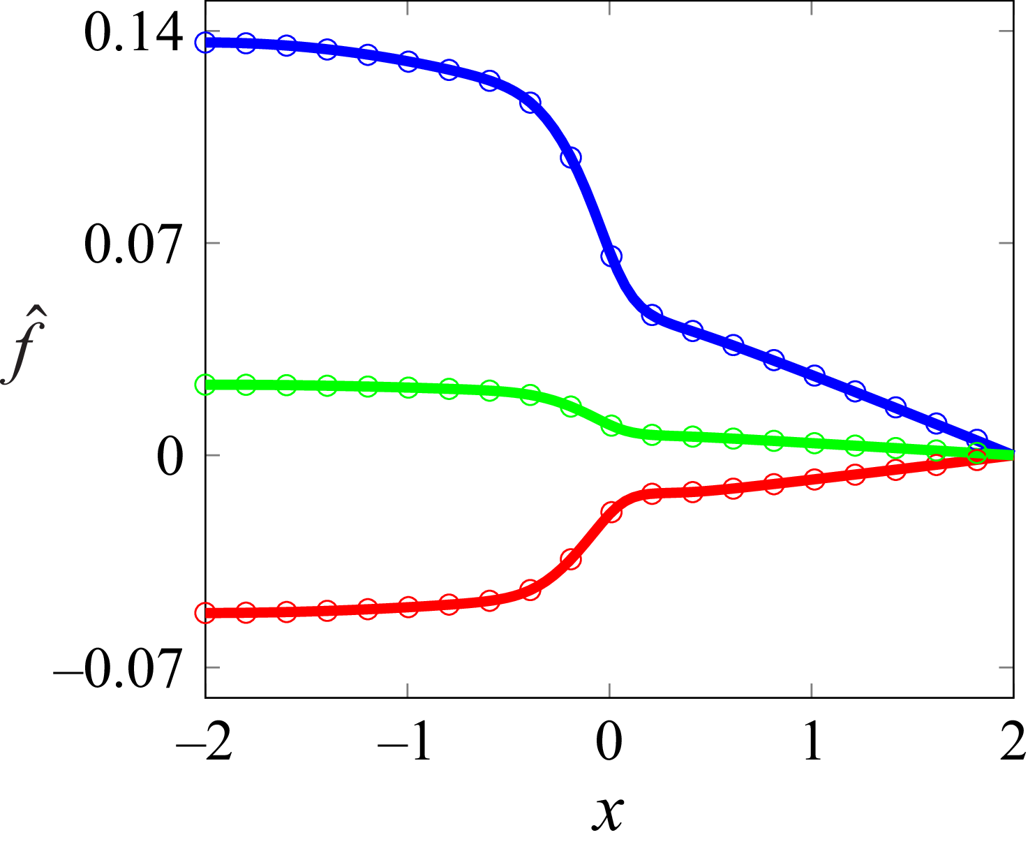
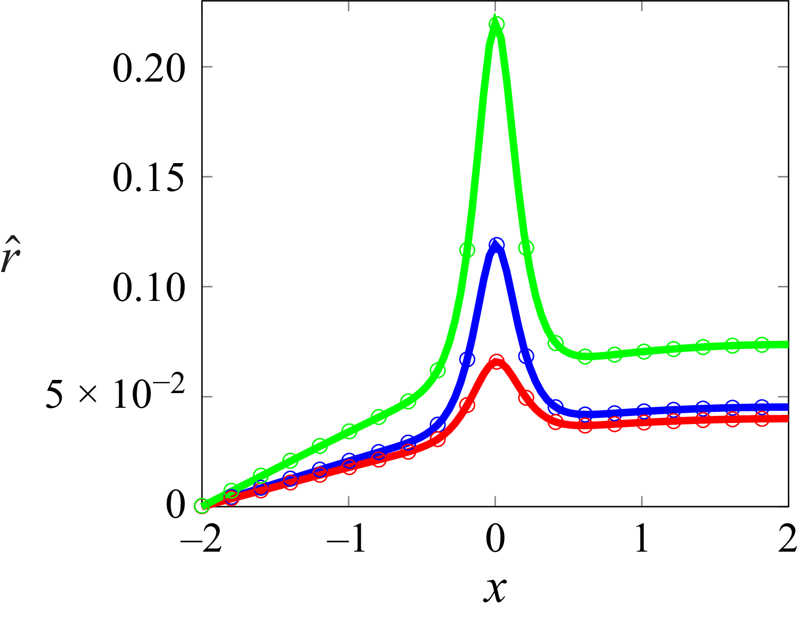
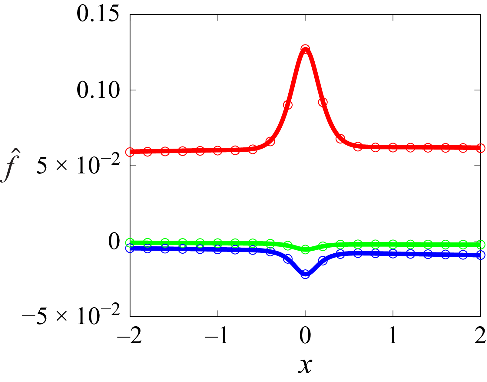
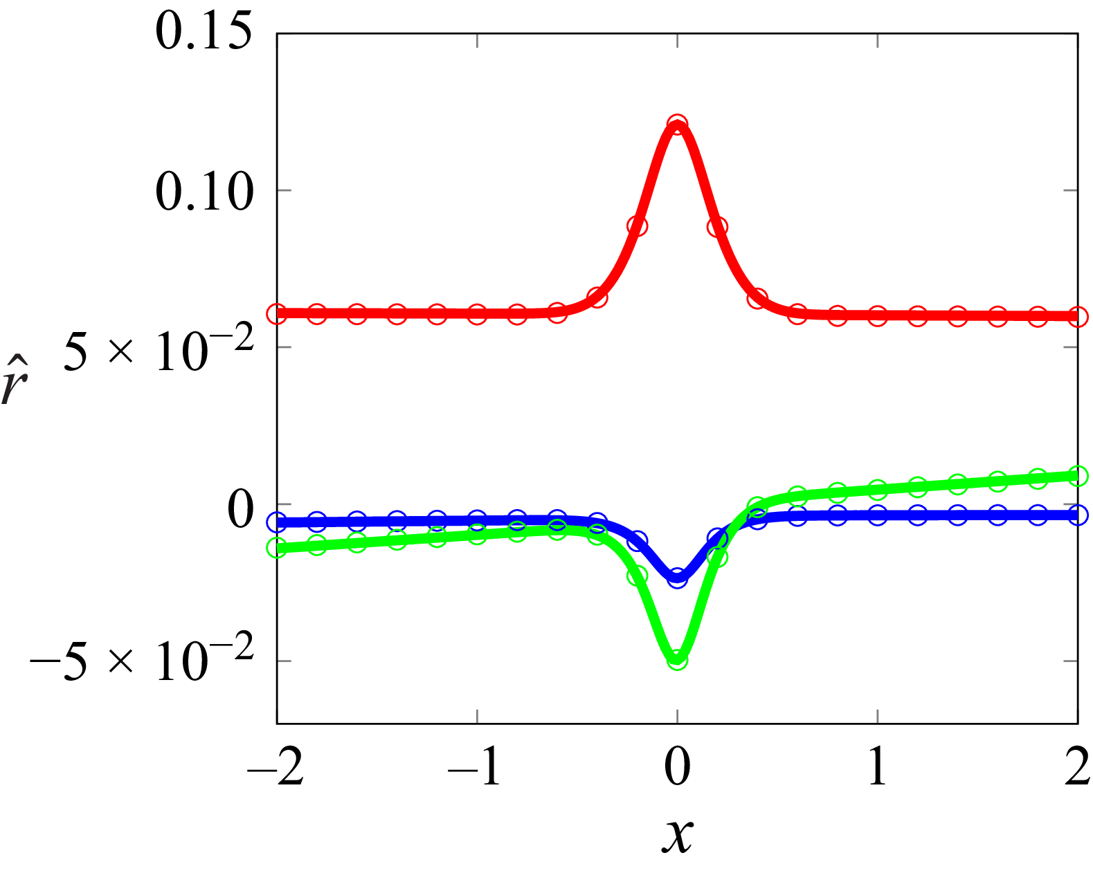
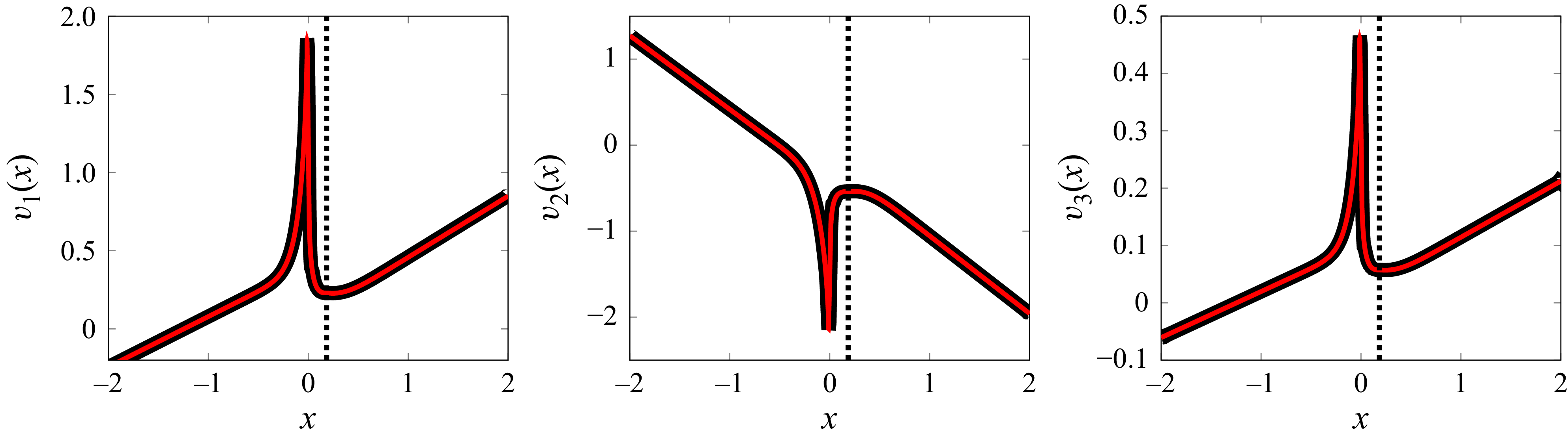
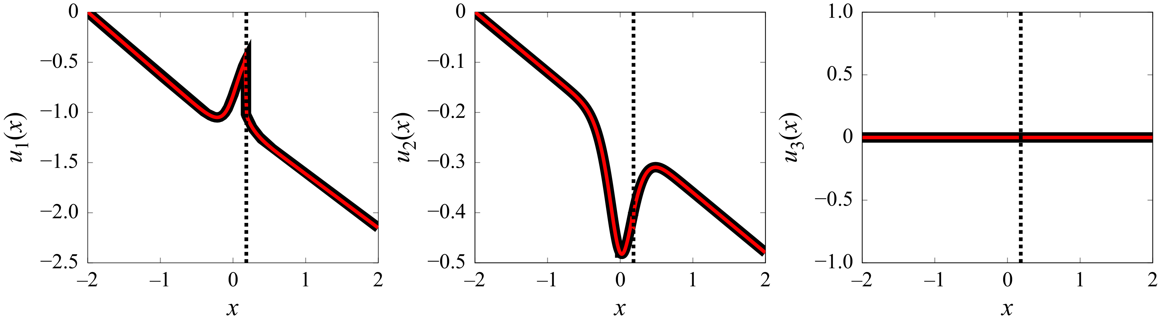

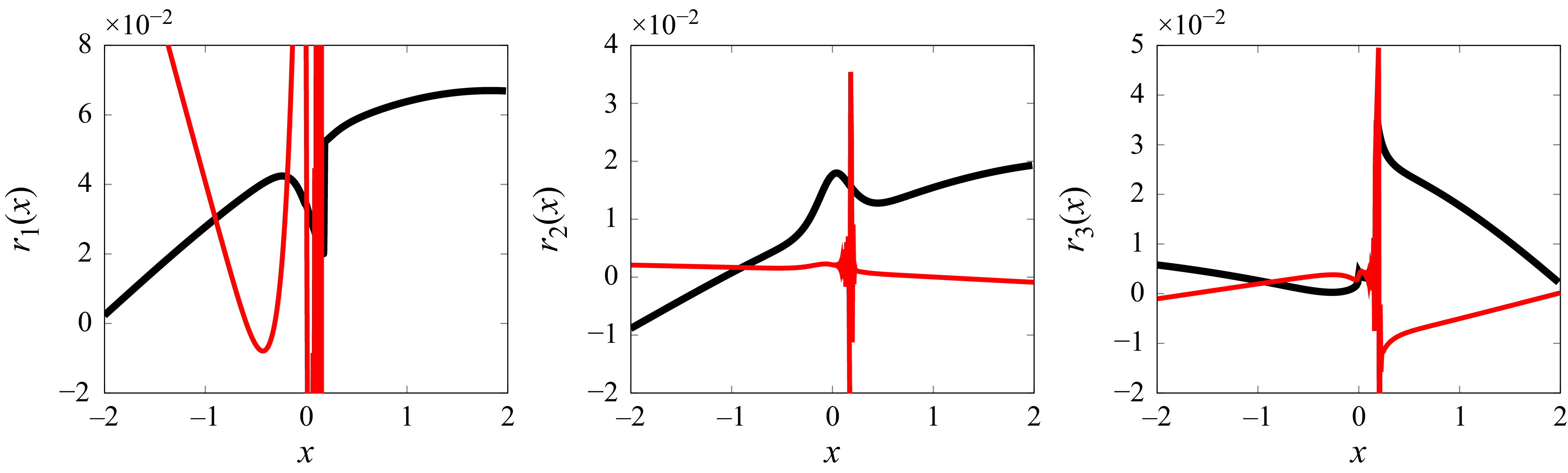
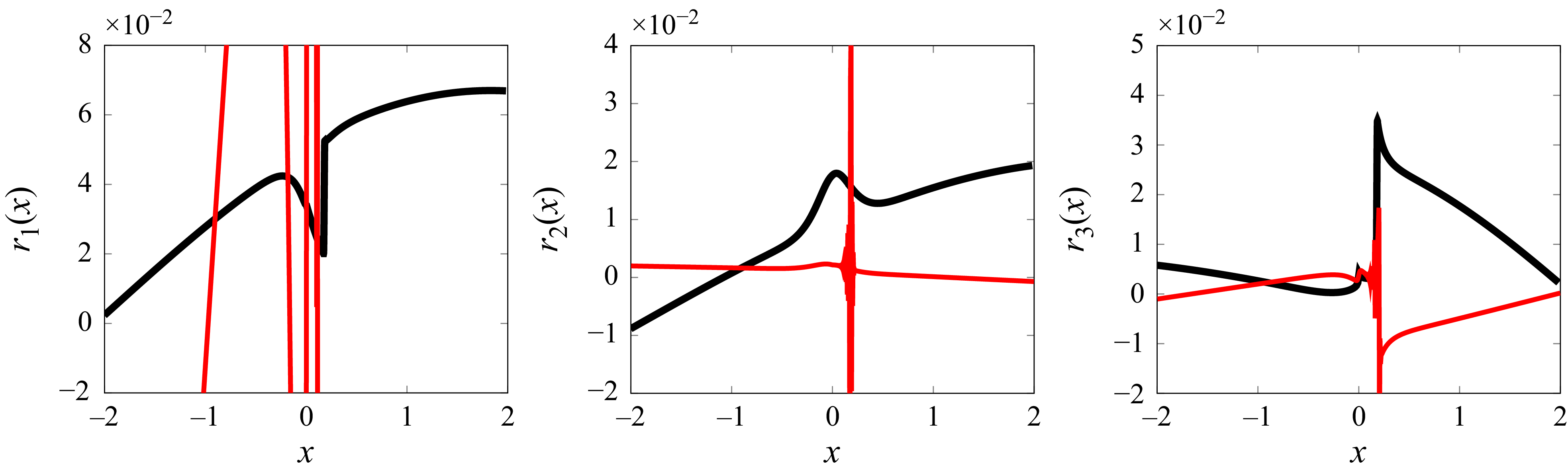


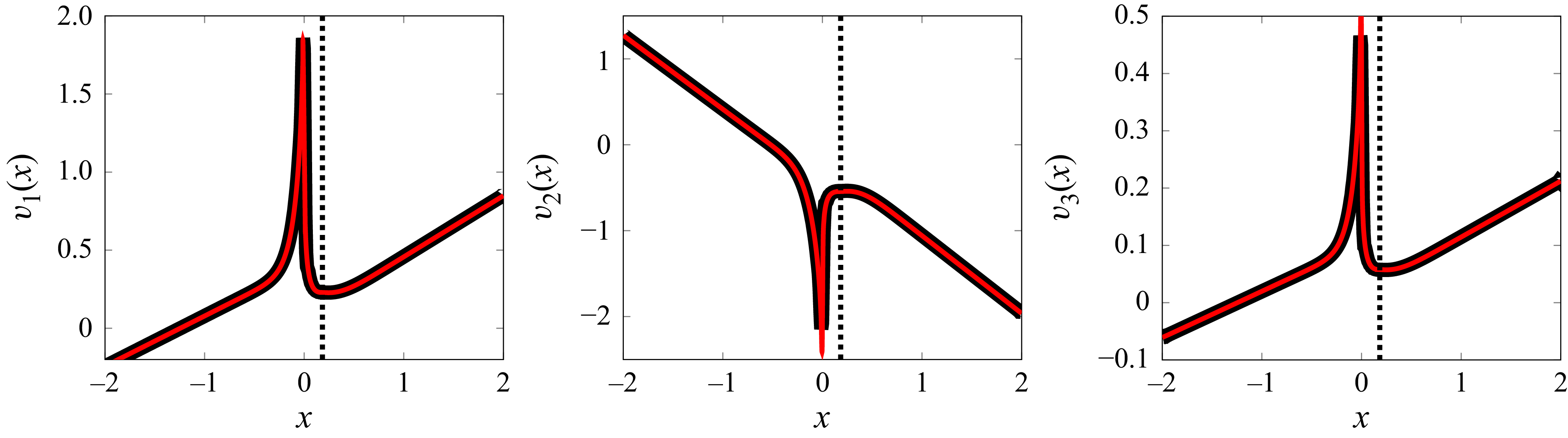
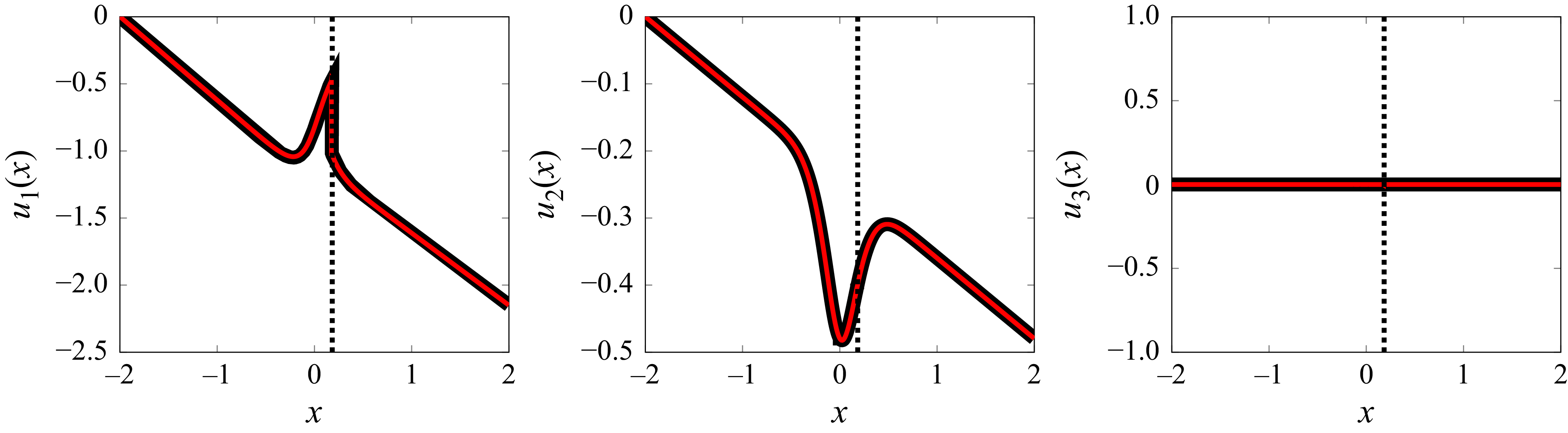

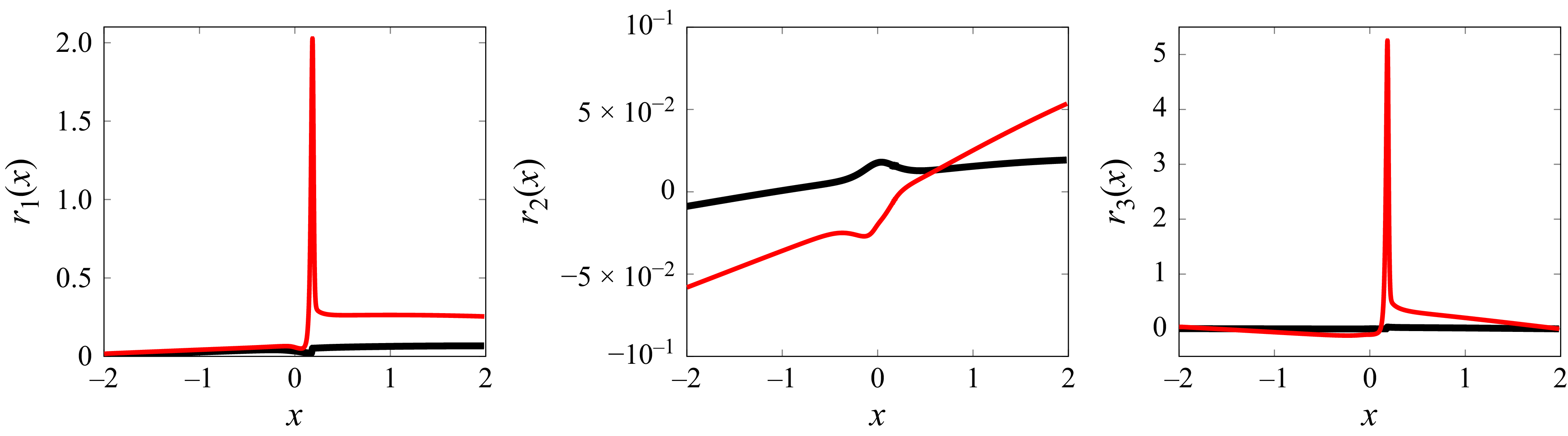

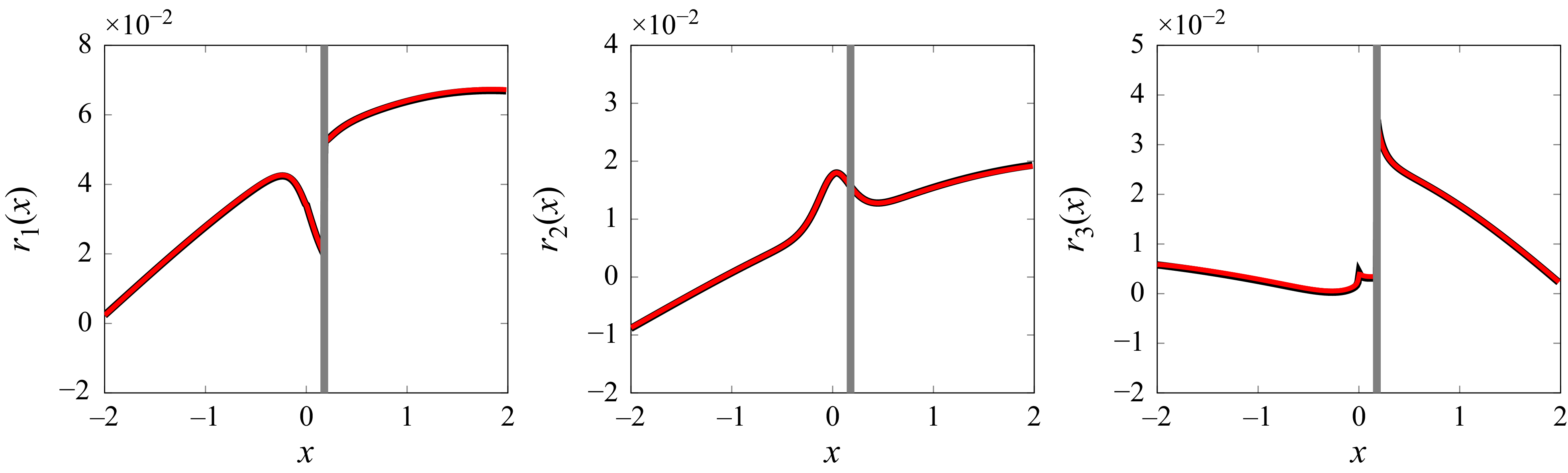
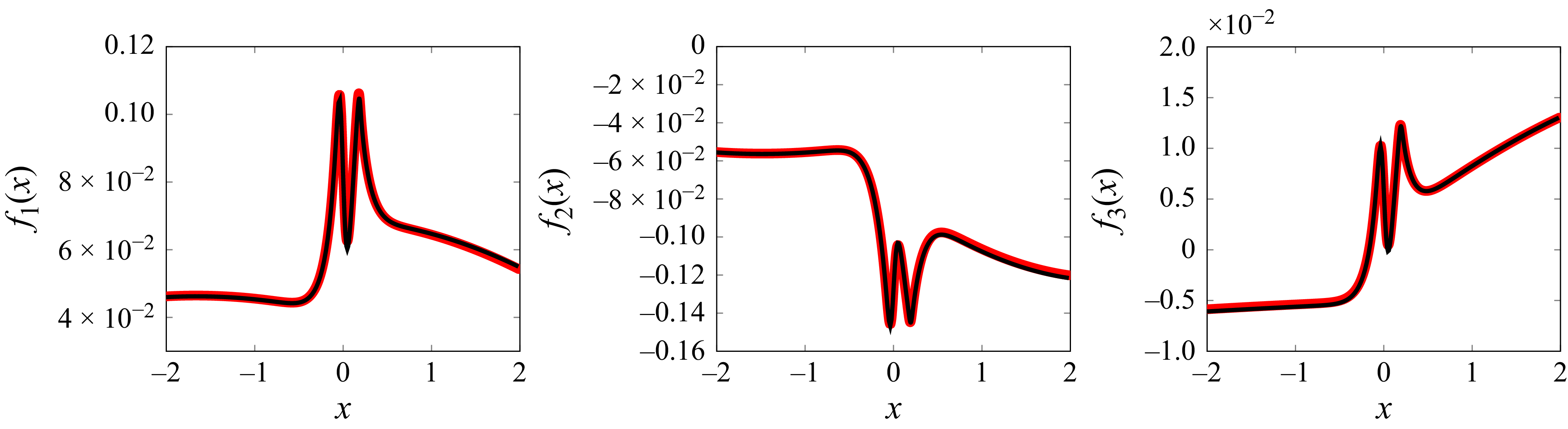

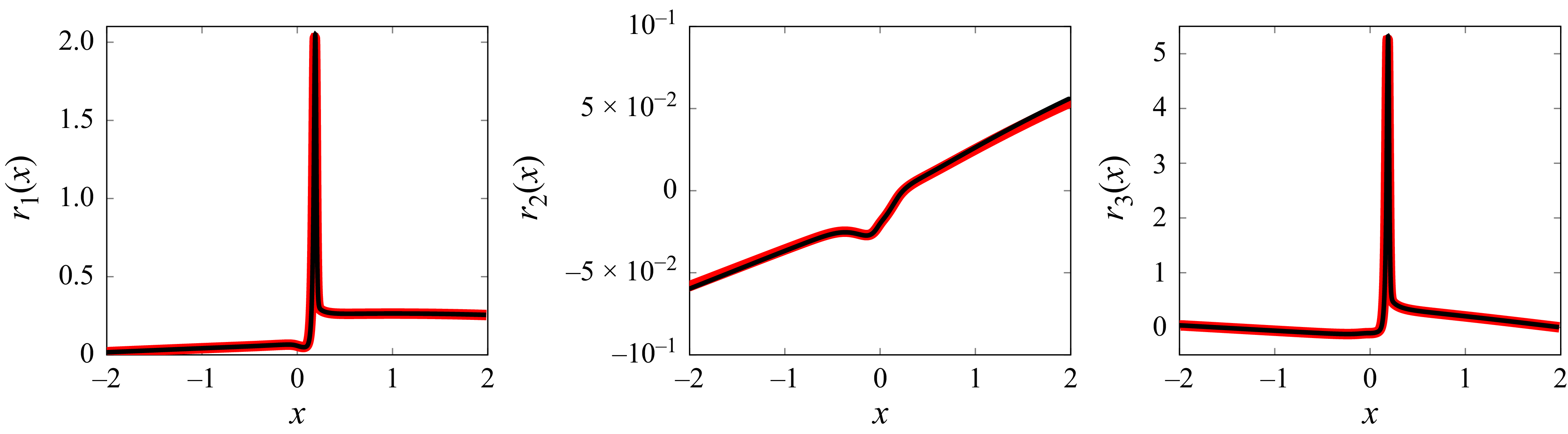

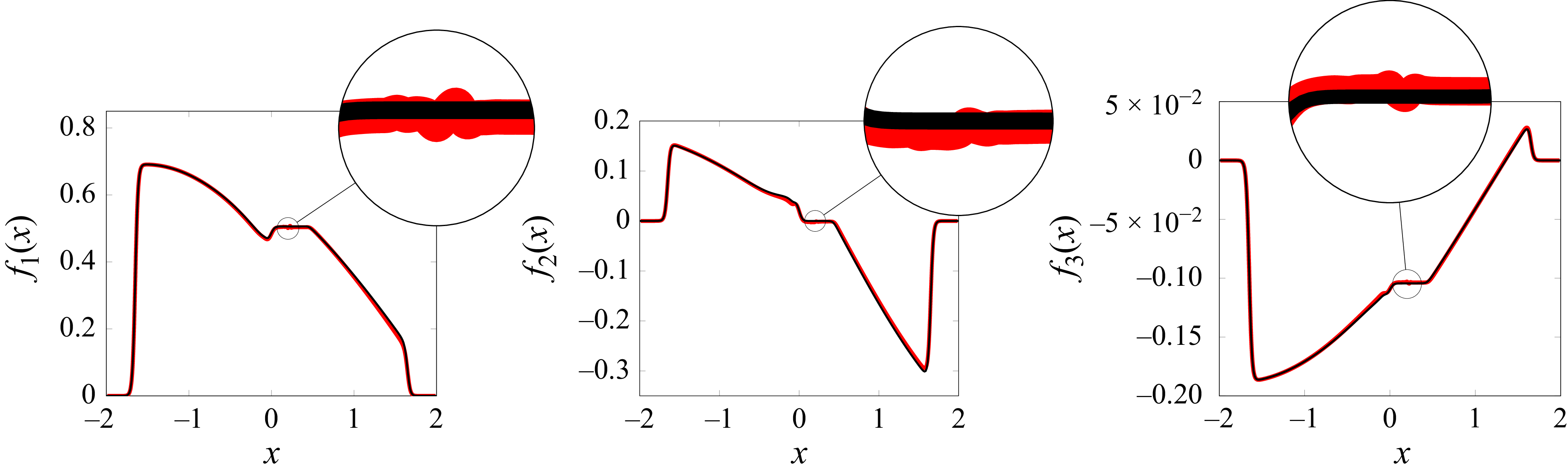

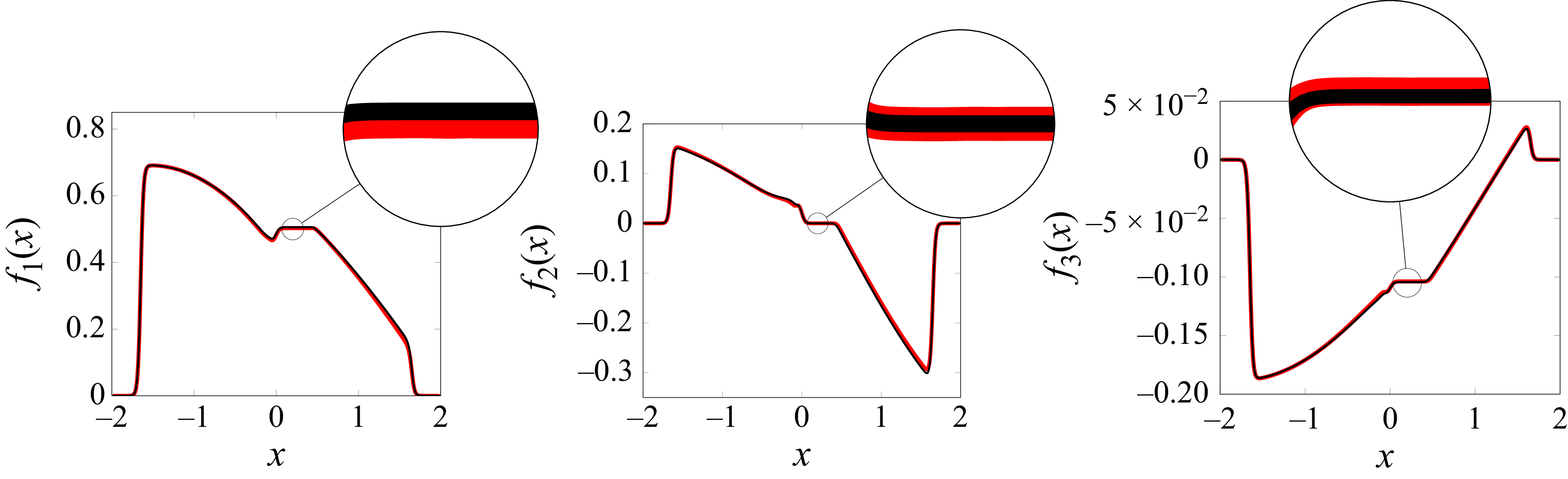

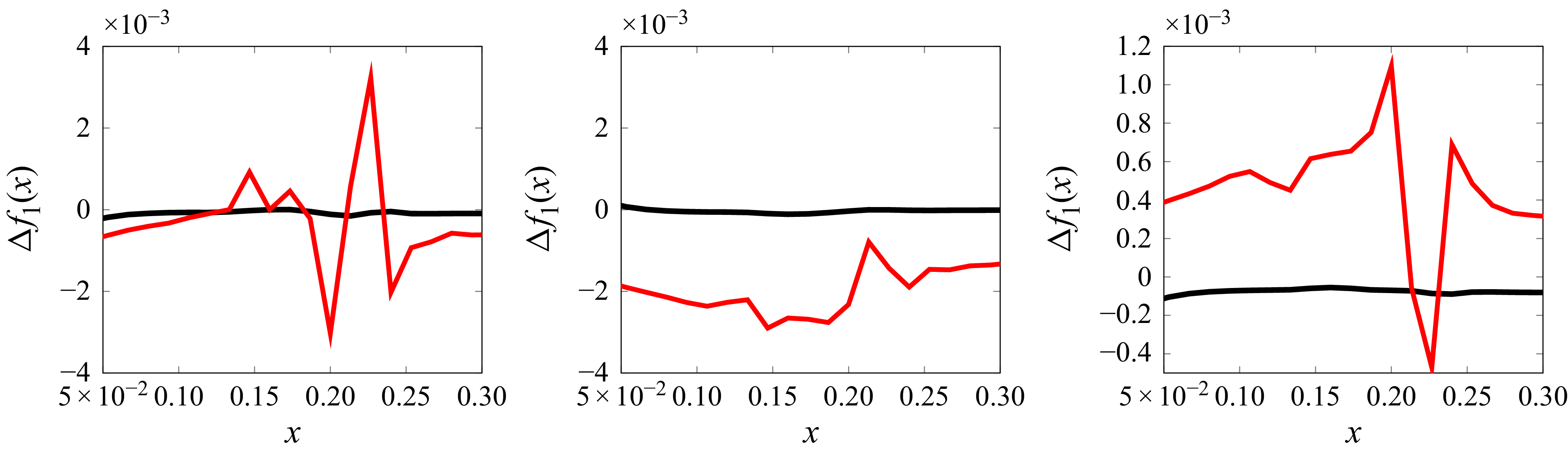


 Open access

