

INTRODUCTION
The Greenland ice sheet is losing mass at an increasing rate (Shepherd and others, Reference Shepherd2012), with the most significant thinning rates observed near the fronts of Greenland's marine terminating glaciers (Csatho and others, Reference Csatho2014). It is hypothesized that these changes are forced from glacier termini (Nick and others, Reference Nick, Vieli, Howat and Joughin2009; Lea and others, Reference Lea2014), placing recent focus on the interactions between marine-terminating glaciers and the ocean. In particular, several studies have explored the role of submarine melt of glacier termini in triggering increased mass loss from the Greenland ice sheet (Holland and others, Reference Holland, Thomas, de Young, Ribergaard and Lyberth2008; Murray and others, Reference Murray2010; Bevan and others, Reference Bevan, Luckman and Murray2012). Understanding the nature of ice/ocean interactions is therefore a primary focus with fundamental implications for ice-sheet loss and sea-level rise (e.g. Straneo and others, Reference Straneo2013).
Despite the overarching signals of coastally-focused mass loss around Greenland (Harig and Simons, Reference Harig and Simons2012) and broad temporal coherence in tidewater glacier terminus retreat (Bjørk and others, Reference Bjørk2012), there is significant spatial and temporal variability that cannot be explained by regional oceanic or atmospheric forcing (e.g., Kjaer and others, Reference Kjaer2012; Straneo and others, Reference Straneo2012). Frequently, neighboring glaciers exhibit contrasting retreat or acceleration behaviors (Moon and Joughin, Reference Moon and Joughin2008; Joughin and others, Reference Joughin, Smith, Howat, Scambos and Moon2010; Moon and others, Reference Moon, Joughin, Smith and Howat2012), highlighting the complexity of tidewater termini processes. There are a number of potential drivers of these observed differences in glacier behavior, including contrasts in heat transport to termini (Sutherland and others, Reference Sutherland, Straneo and Pickart2014), contrasts in subglacial discharge-forced melting (Slater and others, Reference Slater, Nienow, Cowton, Goldberg and Sole2015), and differences in glacier geometry (Carr and others, Reference Carr2015). Calving style (whether through ~104 m3 serac failures (Bartholomaus and others, Reference Bartholomaus, Larsen, O'Neel and West2012) or ~109 m3 iceberg slab rotations (Amundson and others, Reference Amundson2008)) may also be symptomatic of, or responsible for, differences in dynamic glacier behavior (Åström and others, Reference Åström2014).
While improved knowledge of the physical characteristics of neighboring glacier/fjord systems can better guide understanding of the critical, rapidly-changing ice/ocean interface (Straneo and others, Reference Straneo2013), a dearth of observations hampers our ability to isolate the importance of these individual factors. Here, we present new observations and model results providing an integrated, interdisciplinary picture of glaciological and oceanographic contrasts among three glaciers in West Greenland. From north to south, these are Umiammakku Isbræ (‘UI’; in new Greenlandic: Umiammakku Sermiat; 71.7°N, 52.4°W), Rink Isbræ (‘RI’; in new Greenlandic: Kangilliup Sermia; 71.7°N, 51.6°W), and Kangerlussuup Sermia (‘KS’; 71.5°N, 51.4°W) (Bjørk and others, Reference Bjørk, Kruse and Michaelsen2015). Collectively, UI, RI and KS span 100 km of the 250 km ice-sheet margin flowing to the Uummannaq fjords system in west Greenland.
UI, RI and KS glaciers exhibit a range of thicknesses, mean velocities and seasonal velocity variations (Bevan and others, Reference Bevan, Luckman and Murray2012; Moon and others, Reference Moon2014; Morlighem and others, Reference Morlighem, Rignot, Mouginot, Seroussi and Larour2014), as summarized in Table 1. RI flows more than twice as fast as either UI or KS, and is more than three times as thick as either of its neighbors. RI is the seventh largest source of ice discharged from the Greenland ice sheet (Enderlin and others, Reference Enderlin2014). Seasonal surface speeds at RI and UI exhibit a similar pattern and peak late in the year, coincident with a retracted terminus position (Howat and others, Reference Howat, Box, Ahn, Herrington and McFadden2010; Moon and others, Reference Moon2014). Speeds at KS generally exhibit a late summer minimum interpreted to result from the evolution of an efficient subglacial drainage system (Howat and others, Reference Howat, Box, Ahn, Herrington and McFadden2010; Moon and others, Reference Moon2014).
Summary of glacier characteristics

Mean speeds measured 1–2 km from the glacier terminus (Fig. 5). Depth to shallowest sill is the minimum fjord thalweg depth between the glacier terminus and the continental slope. Thickness changes are within 10 km of terminus from differencing ice surface elevations identified in a 1985 aerial photograph-derived DEM with DEMs produced from 2012 to 2013 WorldView images (Felikson and others, in preparation).
§ The shallowest sill for KS glacier is at the glacier terminus, but the shallowest sill depth for the KS fjord, within which we report temperature and salinity (Fig. 3), is 410 m.
* Howat and others (Reference Howat, Box, Ahn, Herrington and McFadden2010).
† McFadden and others (Reference McFadden, Howat, Joughin, Smith and Ahn2011).
‡ Bevan and others (Reference Bevan, Luckman and Murray2012).
|| Moon and others (Reference Moon2014).
Over longer timescales, KS does not exhibit a decadal trend in its velocity or terminus position (Howat and others, Reference Howat, Box, Ahn, Herrington and McFadden2010; Bevan and others, Reference Bevan, Luckman and Murray2012; Moon and others, Reference Moon, Joughin, Smith and Howat2012), yet both RI and UI are undergoing dynamic changes. Between 2003 and 2008, UI retreated, accelerated and thinned, before restabilizing after 2009 (Bevan and others, Reference Bevan, Luckman and Murray2012). In clear contrast to the UI step change, the RI terminus is thinning gradually at 1 m a−1, and has retreated ~1 km since the early 1990s (Bevan and others, Reference Bevan, Luckman and Murray2012).
The disparate seasonal and decadal behavior that UI, RI and KS exhibit, despite occupying the same regional atmospheric and oceanic environment, provides an opportunity to study the key physical relationships and sensitivities internal to the ice/ocean system (Fig. 1). To simultaneously characterize the ice/ocean systems of UI, RI and KS, we couple new field and remotely-sensed observations with numerical modeling. The ultimate goal is to characterize the differing ice/ocean systems and explain the source of these differences. Together, this program provides a foundation for future studies of specific processes and offers insight into the potential factors responsible for the sharp contrasts in dynamic behavior among adjacent glaciers.
Overview of glacier and fjord geometry. (a) Map of the study area showing merged bathymetry and subglacial topography. Thalweg along-fjord profiles (i.e., following the path of least elevation), shown as solid lines with distances from an arbitrary, common point. Dashed lines show the hydrologic catchment boundaries. Glacier velocities during the 2007/08 winter are contoured at 500 m a−1 with dark gray lines; fastest and slowest contours for each glacier are labeled. Diamonds identify the locations of moorings that provided ocean velocity time series presented in Figure 3. The star on the inset map of Greenland shows the location of our study area. Elevations are referenced to the EGM96 geoid. (b) Along-fjord/glacier thalweg cross sections, with key points identified. Glaciers are shaded with consistent line styles for surface and bed elevations.

METHODS
We combine oceanographic and glaciological field observations during the summers of 2013 and 2014 with remote sensing and numerical modeling. These joint approaches enable us to characterize seasonal variability in glacier and ocean dynamics at UI, RI and KS during our observational time period.
Glacier and fjord geometry
The bathymetry of Karrats Isfjord (hereafter “RI fjord”) was mapped in 2009 by the RRS James Clark Ross (cruise JR175) (Dowdeswell and others, Reference Dowdeswell2014). In 2013, we mapped the seafloor in KS fjord using a Reson 7111 multibeam swath bathymeter and made more limited depth soundings along the fjord in which UI terminates (Fig. 1). For land beneath the ice sheet, we draw on the ice sounding radar and mass-conservation-constrained subglacial topography product of Morlighem and others (Reference Morlighem, Rignot, Mouginot, Seroussi and Larour2014) (Fig. 1a; version of 2015-07-30). We merge these data products by gridding all bathymetric measurements to the 150 m resolution of the mass-conserving bed. Where multiple measurements exist within a grid cell, we use the mean elevation for our merged product.
Reported ice thickness uncertainties over the lowest 20 km of UI are 70–120 m. At RI and KS, ice thickness uncertainties are 20–100 m. For the ice surface topography, we incorporate the ice surface elevation dataset of the Greenland Ice Mapping Project (GIMP) (Howat and others, Reference Howat, Negrete and Smith2014), which represents a mean elevation between 2003 and 2009. At the fronts of nearly-stable RI and KS, the GIMP surface elevation is similar to that measured in 2013 (Felikson and others, in preparation). However, the UI terminus has retreated by ~1.2 km from its location in the GIMP dataset and the ice surface elevation is up to 100 m lower at UI in 2013 (Felikson and others, in preparation). At the scale of Figure 1b, these differences are only marginally visible, thus we present unmodified GIMP results.
Fjord water properties and circulation
Detailed ship-based surveys of the water properties within RI and KS fjords were conducted from the R/V Sanna during cruises in September 2013 and July 2014. Shipboard hydrography was collected using a RBR XR-620 conductivity/temperature/depth (CTD) sensor that sampled at 6 Hz. The unit was factory calibrated prior to the cruise. Hydrographic results are reported as potential temperatures and practical salinities. CTD casts within each fjord followed similar patterns. For clarity, we group each cast with others at one of four locations (UI, RI, KS and outside the fjord mouths) and present distributions representing each location (Fig. 2). The outside casts were made within 5 km of the black diamond in Figure 1a. We constrained casts inside the fjords to glacierward of the shallowest sills; for RI and KS this meant plotted casts were within 35 km of the terminus, and for 2013, UI casts were within 12 km of the terminus.
Mean temperature and salinity properties for the UI, RI and KS fjord systems and outside of the fjords during the (a) September 2013 and (b) July–August 2014 cruises. Cross-centers mark the mean temperature and salinity in 2 m depth-binned data; crosses span the standard deviation at each level. In (a), RI data are the average of 25 profiles, KS data average 82 profiles, UI average 44 profiles and data outside the fjords in Uummannaq Bay are the average of 13 profiles. In (b), the corresponding numbers are RI 108 profiles, KS 249 profiles and outside 17 profiles. Isopycnal contours (density in kg m−3–1000) are shown in black. Slopes of the melt (solid) and runoff line (dashed) are indicated. White squares mark depth levels every 100 m; the shallowest 100 m depths are labeled.

Moorings were deployed during the 2013 cruise and recovered in 2014 in order to measure water velocity, temperature and salinity throughout the year-long deployment. Deep-water moorings were deployed along the KS and RI fjord centerlines, and an additional deep water mooring was deployed near the mouth of these fjords, in the broader Uummannaq Bay (diamonds in Fig. 1a). Velocity records were acquired using upward-looking 75 kHz RDI Acoustic Doppler Current Profilers (ADCPs) configured to sample 16 m depth bins every 4 min (Fig. 3). In addition to removing outliers, acoustic correlations and echo intensity were used to remove faulty data returns.
(a) RACMO2.3-estimated subglacial discharge for RI and KS glaciers from September 2013 to August 2014. Along-fjord velocity (m s−1) from (b) RI-deep and (c) KS-deep moorings with positive values representing flow toward the terminus. Circles show the location and magnitude of the daily minimum (black) and maximum (grey) along-fjord velocity. Only values significantly different from zero are selected. During this time period, the moorings were covered by rigid sea ice/melange from early January 2013 to late June 2014. RI fjord is 1080 m deep at the mooring location. The 485 m depth of the KS fjord at the mooring location is identified by the black dotted line.

Subglacial discharge
We utilize downscaled daily RACMO2.3 11 km surface mass-balance products (version v0.2) to estimate subglacial discharge emerging at the terminus of UI, RI and KS (Noël and others, Reference Noël2015). The downscaling procedure reconstructs the surface mass balance at 1 km horizontal resolution by interpolating individual surface mass balance components, including runoff, on the GIMP ice surface elevation and ice mask (Howat and others, Reference Howat, Negrete and Smith2014), using an elevation correction. Due to an insignificant correlation between precipitation and elevation, we apply a bi-linear interpolation to the 1 km precipitation grid without elevation correction. This high-spatial resolution dataset, with daily temporal resolution, is appropriate for use in our high vertical relief study area. We delineate individual glacier catchments for each glacier using a hydropotential surface (Shreve, Reference Shreve1972). In a manner similar to Kienholz and others (Reference Kienholz, Hock and Arendt2013), we manually group watersheds contributing to a single glacier terminus. Downscaled RACMO2.3 runoff values are then extracted within each catchment. At each RACMO2.3 epoch, the field of clipped runoff values is spatially integrated over each catchment to yield a time series of daily subglacial discharge at the terminus of each catchment. The evolving glacial hydrologic system likely modulates and delays the arrival of surface runoff at the terminus (Bartholomaus and others, Reference Bartholomaus, Anderson and Anderson2011; Hewitt, Reference Hewitt2013; Andrews and others, Reference Andrews2014). However, for the purpose of this seasonally-focused study, we assume that runoff arrives instantaneously at the terminus and refer to this spatially integrated product as subglacial discharge throughout this paper (Figs 3a, 4a, 5a).
Seasonal subglacial discharge from the three glaciers and its influence on equilibrium plume depths. (a) Estimated subglacial discharge flux for RI, KS, and UI glaciers during summer 2013 and 2014 (RACMO2.3). (b) Comparison between simulated and observed turbid plume occurrence. Horizontal lines identify time periods when plumes are predicted to reach the surface at the terminus due to momentum-driven overshoot, based on the plume model implemented in Carroll and others (Reference Carroll2015). Symbols identify satellite observations: open circles represent times when plumes were absent, squares represent periods of sea ice/melange cover, and filled circles represent when plumes were observed in satellite-based imagery. (c) Predicted neutrally-buoyant plume outflow depth down-fjord from the terminus; error bars represent uncertainty (two standard deviations) due to variability in ambient fjord stratification. Hydrographic data from RI was used to initialize the UI plume model during summer 2014, when temperature/salinity observations inside UI are lacking.

Subglacial discharge (downscaled, spatially-integrated RACMO2.3), glacier centerline terminus velocities 1–2 km behind the glacier terminus, and mean terminus length (arbitrary datum) for UI, RI and KS during 2013 and 2014. In all panels, UI is green, RI is red and KS is blue. In August 2014, speeds at KS fall to 500 m a−1 and remain at that level until late September (for two measurements).

Evidence of subglacial discharge from tidewater glaciers is sometimes apparent at the fjord surface in the form of turbid plumes emerging from the glacier terminus (Chu and others, Reference Chu, Smith, Rennermalm, Forster and Box2012). We quantify the timing and location of sediment-laden plumes originating from the glacier terminus by manually inspecting 51 Landsat 7, Landsat 8 (30 m resolution) and Advanced Spaceborne Thermal Emissivity and Reflection Radiometer (ASTER; 15 m resolution) images during the 2013 and 2014 melt seasons. The average temporal resolution of our satellite observations is 1.5 weeks (Fig. 4b).
We compare the occurrence of turbid surface plumes at glacier termini with model-derived estimates for subglacial plume depths (Carroll and others, Reference Carroll2015). This plume model assumes subglacial discharge emerges from a single subglacial conduit at the grounding line, resulting in a turbulent plume that rises along the vertical ice face. Given a subglacial discharge flux at each of UI, RI and KS, we estimate the times when the momentum-driven plume should appear on the fjord surface (maximum height) and the depth at which the plume should equilibrate as it moves down-fjord (outflow depth) (Fig. 4c).
Glacier velocities and force balance
Satellite radar and optical imagery are used to derive ice velocity for RI, KS and UI. We predominantly use TerraSAR-X imagery (© DLR 2013; © DLR 2014), following techniques outlined by Joughin and others (Reference Joughin, Smith, Howat, Scambos and Moon2010). Ice velocity fields are produced using 11 or 22 d repeat interferograms gridded to 100 m horizontal resolution. The average error in velocity near the terminus of these three glaciers is 14 m a−1 on RI and 3 m a−1 on UI and KS, or 0.2% of their total speeds. Earlier velocity data from RADARSAT during the 2007/08 winter (Fig. 1a) indicate that spatial patterns in velocity have remained stable in recent years.
We supplement the TerraSAR-X velocity record using a standard feature tracking technique on sequential Landsat 8 panchromatic imagery (15 m resolution) (e.g. Stearns and others, Reference Stearns2015). These results have slightly higher errors that scale with the time separation of the two images (40 m a−1, on average) but compare well with overlapping TerraSAR-X data. From these TerraSAR-X and Landsat velocity fields, we extract time series of speeds for each glacier at locations 1–2 km behind the glacier terminus (Fig. 5b). A list of the TerraSAR-X and Landsat scenes used for this analysis are given in supplementary Table S1.
Insight into the large-scale mechanisms controlling glacier motion can be obtained from calculations of the stresses that drive and resist flow. We employ the force budget technique described by van der Veen and Whillans (Reference van der Veen and Whillans1989) to calculate forces at depth using measurements of surface velocity and estimates for surface slope and ice thickness (Howat and others, Reference Howat, Negrete and Smith2014; Morlighem and others, Reference Morlighem, Rignot, Mouginot, Seroussi and Larour2014). The driving stress is responsible for making ice flow in the downslope direction; resistance to flow can come from the bed (basal drag), the sides (lateral drag), or along-flow obstacles (longitudinal stress gradients). Similar methods have been used at Columbia Glacier, Alaska (O'Neel and others, Reference O'Neel, Pfeffer, Krimmel and Meier2005), Byrd Glacier, Antarctica (van der Veen and others, Reference van der Veen, Stearns, Johnson and Csatho2014) and Jakobshavn Isbrae, Greenland (van der Veen and others, Reference van der Veen, Plummer and Stearns2011) to understand controls on ice flow.
To calculate the force balance for our region of interest, we use surface and bed topography from Morlighem and others (Reference Morlighem, Rignot, Mouginot, Seroussi and Larour2014), available at 150 m grid spacing. We use an ice velocity product available at the same grid spacing, from Rignot and Mouginot (Reference Rignot and Mouginot2012). This product compiles interferometrically-derived ice velocities from different sensors between 2008 and 2009. Force balance calculations were also done for each glacier using velocities derived for 2013/14, which yield similar results. However, since the spatial extent of the 2013/14 velocity data are smaller, we show results for the whole region using 2008/09 data (Figs 6, 7). We use a rate factor of B = 400 kPa a1/3, corresponding to a depth averaged ice temperature of −10°C, following borehole measurements and similar modeling studies at Jakobshavn Isbrae 300 km to the south (Luthi and others, Reference Luthi, Funk, Iken, Gogineni and Truffer2002; Thomas, Reference Thomas2004; van der Veen and others, Reference van der Veen, Plummer and Stearns2011). Results are smoothed by a 1 km gaussian kernel to remove noise.
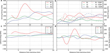
Force budget for our study region. (a–d) are the components of the depth-averaged force balance (van der Veen and Whillans, Reference van der Veen and Whillans1989); (e) is basal drag from inversion of ISSM (Larour and others, Reference Larour, Seroussi, Morlighem and Rignot2012). Scale for panels (a–e) is the same. (f) Larger-scale views of the basal drag at RI and KS, calculated using both the force balance (FB) and ISSM approaches. All panels are plotted with the same colorbar.

We also use the Ice Sheet System Model (ISSM; Larour and others, Reference Larour, Seroussi, Morlighem and Rignot2012) to invert for basal drag from surface velocities by a control method (e.g. MacAyeal, Reference MacAyeal1993). Our inversion uses higher-order ice dynamics (Blatter, Reference Blatter1995; Pattyn, Reference Pattyn2003) that include vertical shearing in addition to the forces considered in the van der Veen and Whillans (Reference van der Veen and Whillans1989) method. Because ISSM applies observed velocities as (essential) boundary conditions, lateral drag is not explicitly calculated. We run the model over our study domain (Fig. 1) with ten vertical layers, very slightly concentrated towards the bed (with the first four in the bottom 27% of the glacier). We impose a uniform ice temperature of −10°C to ease comparison with the vertically-integrated force balance technique (Figs 6, 7).
Calving and seasonal change in terminus position
Glacier termini are traced from Landsat (Level 1T) and TerraSAR-X imagery following techniques outlined by MacGregor and others (Reference MacGregor, Catania, Markowski and Andrews2012). While the Landsat products were consistently georeferenced correctly, some of the raw TerraSAR-X scenes had poor registration and had to be manually georeferenced relative to the Landsat scenes to ensure consistent terminus position mapping (all TerraSAR-X ice velocity products were automatically georeferenced). From this compilation of terminus traces we compute the change in glacier area between successive traces, the fjord walls and an arbitrary upstream gate. These terminus areas are then normalized by the glacier terminus widths (Table 1). Thus, these terminus positions characterize changes in mean glacier length rather than centerline length changes (Fig. 5c). Centerline length changes are generally larger than mean length changes at our study glaciers.
PHYSICAL CHARACTERISTICS OF ADJACENT GLACIERS AND FJORDS
Glacier and fjord geometry
Both RI and KS terminate in 60 km-long fjords that open onto the broader Uummannaq fjord system. UI fjord branches from RI fjord roughly halfway between the fjord mouth and the RI terminus. One of the clearest contrasts among these different glacier/fjord systems is their ice thicknesses and fjord depths (Fig. 1). RI fjord is ~1100 m deep over much of its length (Dowdeswell and others, Reference Dowdeswell2014), whereas the KS and UI fjords are much shallower with depths of ~500 and 350 m, respectively. The widths also vary; the RI and KS fjords are both ~6 km wide, whereas the UI fjord is ~3 km wide. Both RI and KS fjords have relatively shallow sills (430 and 410 m for RI and KS fjords, respectively) near their entrances (at 15–30 km in Fig. 1b for KS and at 26 km for RI). Several ~250 m deep sills cross UI fjord between where it branches from RI fjord and the UI terminus.
RI has a deep grounding line at 840 m below sea level; KS's grounding line is 250 m below sea level. UI's grounding line is 230 m below sea level. Both KS and UI terminate on local bathymetric highs that rise 100 and 200 m, respectively, above the neighboring sea floor. For each terminus, we identify any ungrounded area by calculating the terminus height above flotation (van der Veen, Reference van der Veen1996) using the surface and ice thickness datasets (Howat and others, Reference Howat, Negrete and Smith2014; Morlighem and others, Reference Morlighem, Rignot, Mouginot, Seroussi and Larour2014). While both KS and UI are grounded everywhere at their termini (positive heights above buoyancy), RI has a 9 km2 area on the southeast side of its terminus where the ice surface is up to 50 m below its neutrally buoyant elevation. We hypothesize that buoyant, upward-directed, bending stresses in this ungrounded region lead to the expansion of basal crevasses and promote full-thickness, bottom-out calving events (Murray and others, Reference Murray2015). Three bottom-out calving events were observed in the field at RI during the summer of 2014, similar in style to those that occur at Helheim Glacier, on the southeast coast of Greenland (James and others, Reference James, Murray, Selmes, Scharrer and Leary2014; Murray and others, Reference Murray2015). Comparison between the glacier bed depth calculated from ice flow continuity (Morlighem and others, Reference Morlighem, Rignot, Mouginot, Seroussi and Larour2014) and fjord bathymetry (Dowdeswell and others, Reference Dowdeswell2014) indicates that the 9 km2 ocean cavity beneath ungrounded RI reaches up to 220 m in height (Fig. 1).
Fjord water properties and circulation
The UI, RI and KS fjord systems are characterized by markedly different hydrographic conditions, as illustrated by their temperature-salinity (TS) properties (Fig. 2). Most notable is the degree to which TS properties within each fjord are related to those outside the fjords in Uummannaq Bay (labeled Outside in Fig. 2). At depths >100 m, KS fjord waters were most similar to the outside waters, RI water was somewhat more different and UI water properties (which branch from RI and were only measured during the fall 2013 cruise), were most different.
Within all fjords and during both cruises, the near surface waters (densities <1026.5–1026.8 kg m−3) are cooler and fresher than the water outside the fjords, however the thickness of this surface water varied from fjord to fjord and between cruises. During fall 2013, this colder-fresher water layer extended to 50–60 m depth at RI and UI and to 100 m depth at KS. During the summer 2014 cruise, this surface water extended only half as deep, to 30 m at RI and 50 m at KS. If these cruises are considered samples of a seasonal cycle, then the amount of colder-fresher water accumulates at the surface over the course of the summer melt season, thickening this layer. Further differences in the shallowest water among fjords are likely the result of local atmospheric influences (e.g. katabatic wind strength), subglacial discharge, fjord wall runoff and ice melange melting and mixing through calving events and the overturning of floating icebergs.
Deeper than these shallowest 50–100 m water depths, the KS profiles were quite similar to the outside profiles, but the RI and UI profiles were warmer and fresher down to depths of 300 m. Below 300 m depth, the RI, KS and outside profiles cannot be distinguished due to the variability intrinsic to each of these three locations. Within the intermediate (~50–300 m) depths of RI, the water is generally 0.25–1.25°C warmer for a given salinity class (or depth) than outside. The difference from the outside water was greater during the summer 2014 cruise, than during the fall 2013 measurements, largely due to colder shallow (~50 m depth) water outside the fjords during summer 2014. As with the shallowest water layers, these contrasts may reflect seasonal or interannual variability. However, in contrast with the accumulation of colder-fresher surface water over the melt season, the warmer-fresher intermediate depth water in RI may be most pronounced instantaneously, at the height of the melt season. During the fall 2013 observations, the mid-depth water in the outside profiles is warmer than that found in KS. Potentially, this reflects advection of warm water out from RI, but which has not extended into the KS fjord. Below 300 m depth, both fjords and outside waters have TS properties that converge to the warm, salty Atlantic-origin water with a temperature near 3°C and a salinity of ~34.5, very similar to fjord waters found just south in Ilulissat Icefjord in front of Jakobshavn Isbrae (Straneo and others, Reference Straneo2012; Gladish and others, Reference Gladish, Holland, Rosing-Asvid, Behrens and Boje2015).
Chauché and others (Reference Chauché2014) previously reported TS properties from within RI fjord obtained from limited surveys in August 2009 (5 profiles) and August 2010 (7 profiles). Their data show similar TS structure to those reported here in RI (Fig. 2b), although the departure point from the runoff line was considerably more shallow in their surveys, at 200 m compared with 300 m. Similar warm, subsurface water masses have also been inferred from TS properties at depths from ~200 to 300 m for several other Greenland systems, including Sermilik Fjord and Kangerdlugssuaq Fjord in SE Greenland (Straneo and others, Reference Straneo2012; Sutherland and others, Reference Sutherland, Straneo and Pickart2014). The TS properties in KS fjord (Fig. 2) are distinct from these deeper fjords, and lack this subsurface warmth.
Acoustic Doppler velocity data from 2 year mooring deployments also show strong differences between the neighboring fjords (Fig. 3). RI is a relatively energetic system with along-fjord velocities regularly exceeding 0.15 m s−1 and a mean maximum speed of 0.10 m s−1 (Fig. 3b). The vertical structure is complex, being characterized by one to two reversals, and varies through the year. Deep flow is typically directed toward the terminus, while flow away from the terminus occupies mid depths (200–500 m) through the fall and winter, and the upper portion of the measured water column (<300 m depth) in mid- to late-summer. The depths of this outflowing water coincide with the depths of the warmer-than-outside water within RI fjord. Velocity variance is elevated during summer compared with the January–June period when both fjords are capped with sea ice and melange. The magnitude of the down-fjord flow is strongest in July–August when the flow is surface intensified. Down-fjord flow weakens in winter as it becomes more subsurface.
In contrast to RI, the KS mooring measured relatively weak flow that was primarily directed toward the terminus year round. Maximum values rarely exceeded 0.08 m s−1 and the annual mean maximum speed was just 0.04 m s−1, less than half of the RI value (Fig. 3c). The along-fjord flow in KS exhibited little vertical structure or variability throughout the year. With the exception of the April–June 2014 time span, when the maximum up-fjord signal was near 250 m depth, the location of the maximum up-fjord flow can be found throughout the water column without a clear, discernable pattern. In order to conserve mass, outflow in KS must occur either in the upper 50 m, or in a return flow along the side of the fjord. Our model results, described in the next section (Fig. 4), suggest the former explanation is more likely.
Subglacial discharge and its impact at the terminus
Significant discharge (>5 m3 s−1) initiated at the beginning of June and terminated in mid- to late August at all three glaciers in 2013 and 2014 (Fig. 4a). Peaks in subglacial discharge occur within 1 d of each other across the neighboring systems. These discharge maxima are generally more extreme for RI and KS than for UI. For example, the largest melt event within the time series (29 July 2013) increased discharge by ~185 and 400% for the RI and KS catchments over 2 d, whereas discharge within the UI catchment increased by just 87%. Subglacial discharge is typically smallest at UI and greatest at RI. This likely occurs because UI is steep and constricted with narrow fjord walls; it has a comparatively small area in low elevation (high melt) zones (Fig. 1b). In contrast, RI is wide, with a large area at low elevations.
Turbid surface plumes are regularly observed between late June and August in optical satellite imagery of KS and UI (Fig. 4). KS tends to be free of ice during summer months, allowing for ready detection of surface plumes. In contrast, the UI fjord typically remains packed with ice late into the summer and melt plumes form polynyas in the melange. In both systems, the plumes regularly form at particular locations in both years, suggesting discharge from a dominant, persistent subglacial channel. The opening to such a dominant channel has been imaged in the submarine terminus of KS (Fried and others, Reference Fried2015). Visible surface plumes at RI are much less frequent and are absent during 2014.
Previous investigators (Jenkins, Reference Jenkins2011; Sciascia and others, Reference Sciascia, Straneo, Cenedese and Heimbach2013; Carroll and others, Reference Carroll2015) have used numerical models and buoyant plume theory to simulate turbulent meltwater plumes rising along a vertical ice face. These models indicate that an upwelling plume's vertical momentum will lead to an overshoot of the level of neutral buoyancy (e.g. Carroll and others, Reference Carroll2015) (Fig. 4b). In the field, this pattern is manifest as a turbid surface expression near the glacier that subsequently rebounds and flows out of the fjord either at subsurface depths (without surface expression) or near the fjord surface (apparent in satellite imagery as a stream of turbid water extending several km down-fjord, e.g. Bartholomaus and others, Reference Bartholomaus, Larsen and O'Neel2013). Here, we use the point source plume model described in Carroll and others (Reference Carroll2015), combined with time-dependent RACMO2.3 discharge data, to estimate an outflow depth (level of neutral buoyancy) and the maximum plume height obtained during the momentum-driven overshoot. Large subglacial discharge fluxes, released at shallow depth from focused subglacial channels, into weakly stratified fjords lead to the shallowest outflow depths. Based on discharge and stratification observed during summer 2013, the plume model suggests surface plumes at the UI and KS termini for 69 and 67 d, respectively (colored lines in Fig. 4b). In contrast, the plume model simulates a surface plume for only 10 d in RI. During 2014, the predicted occurrence of surface plumes observed at the UI, RI and KS termini increased to 77, 49 and 76 d. Observed presence of surface plumes based on satellite observations is consistent with model predictions of plume surfacing with the exception of RI (open and filled symbols in Fig. 4b).
The emergence depth of subglacial discharge at the grounding line results in striking differences in the predicted outflow regimes between the fjords. Plumes in RI produce subsurface outflows, with KS and UI outflows constrained primarily to the upper 50 m (Fig. 4c). During the 2013 summer melt season, the mean outflow depths for UI, RI and KS are 25, 193 and 12 m. For 2014, the mean outflow depths for UI, RI and KS are 16, 148 and 22 m. In deeply-grounded fjords such as RI, the turbulent plume entrains dense Atlantic Water, often resulting in plumes that reach neutral buoyancy well below the surface despite higher discharges at RI than either of UI or KS. For shallower UI and KS fjords, the plume often remains positively buoyant throughout the entire water column, resulting in surface outflows (Fig. 4c). The difference in outflow depths between RI and KS under periods of equivalent subglacial discharge, demonstrates that the combination of grounding line depth and ambient temperature-salinity properties are primary controls on the depths of glacial outflow in these systems.
Glacier velocities, terminus positions and force balance
The three glaciers in our study region exhibit contrasting seasonal dynamics (Fig. 5). RI and UI both exhibit summer speedups of ~500 m a−1, although the relative speed increase is greater at UI due to its lower mean speed. In summer 2013, the onset of the speedup occurred in early May, prior to the onset both of RACMO2.3-predicted runoff or ice melange breakout, which occurred at RI between 12 and 27 June as observed in Landsat imagery. During this time period, RI advanced while UI maintained a steady terminus position. Both RI and UI returned to their pre-summer speeds at the conclusion of the melt season. While UI speeds remained steady throughout the 2013/14 fall, winter and spring, RI slowed by an additional 200 m a−1, while its terminus advanced. Both Howat and others (Reference Howat, Box, Ahn, Herrington and McFadden2010) and Moon and others (Reference Moon2014) report that RI typically attains its peak speed while the terminus is most retracted during the fall. The 2013 summer response to melt at RI is unusual, but the fall 2014 velocity response appears to better follow the more common pattern (Howat and others, Reference Howat, Box, Ahn, Herrington and McFadden2010; Moon and others, Reference Moon2014). Prior to the 2003–2008 retreat of UI, Howat and others (Reference Howat, Box, Ahn, Herrington and McFadden2010) report that UI often attained its maximum speed simultaneously with high melt. Overall, the seasonal variability in velocity is small at RI (~12%) compared with other large outlet glaciers in Greenland (both Jakobshavn Isbræ and Helheim Glacier have seasonal cycles closer to 30%) (Joughin and others, Reference Joughin2012).
KS exhibits velocity variations opposite to those of UI and RI in both their sign and their magnitude (Fig. 5b). In 2013, KS decelerated by 200 m a−1 during the early to mid-melt season. The glacier rebounded to its winter speed by October and slowly accelerated until the middle of the melt season in 2014, when it underwent a dramatic deceleration, with velocities falling to 500 m a−1 (a 75% decrease) over the last 10 km of the trunk.
Contrasts in glacier terminus positions are also apparent (Fig. 5c). All three glaciers share a seasonal advance and retreat cycle, however their timing and magnitude differ significantly during our observation period. KS and UI reached their maximum extent in early June of both 2013 and 2014 and initiated retreat at the start of summer, when runoff increased. The pattern of winter advance and summer retreat (synchronous with subglacial discharge) is similar to patterns commonly observed at other Greenland and Alaskan tidewater glaciers (Howat and others, Reference Howat, Box, Ahn, Herrington and McFadden2010; McNabb and Hock, Reference McNabb and Hock2014; Moon and others, Reference Moon, Joughin and Smith2015). The maximum seasonal extent at RI also occurs between April and June, but with smaller and higher-frequency advance/retreat cycles superimposed. The higher-frequency terminus variations reflect full-thickness, capsizing slab and rifting tabular calving events, which occur approximately every 2.5 months and are characterized by multi-month advances and single or multi-day retreat events. These calving events occur throughout the year. RI advanced 200 m past its 2013 extent in 2014, after which point, the occurrence rate and size of large calving events increased. At RI, the advance rate between capsizing slab calving events is roughly constant, at a mean rate of 2400 m a−1. This is slightly lower than the cross-sectional average terminus speed of 3200 m a−1, indicating that smaller calving events (i.e. serac failures) also play an important role in RI's frontal mass loss. The terminus position records at KS and UI lack dramatic retreats, nor have we observed full-thickness tabular or capsizing icebergs calving from these termini. These glaciers calve through serac failures.
Thick ice and a steep surface slope at RI lead to a high driving stress and fast flow (Figs 6a, 7a). Neighboring glaciers UI and KS are thinner, slower and have smaller driving stresses over the last 10 km of their length. Despite the different magnitudes in forces, the main resistance to flow on all three glaciers comes from friction at the bed (Figs 6d–f). Both lateral drag and longitudinal stress gradients provide minimal resistance to flow, except in localized regions. Compressional flow at the base of a large bedrock high near the terminus of RI causes substantial, yet isolated, resistance from longitudinal stress gradients. Our basal drag inversion using ISSM produces similar results except near relatively steep slopes where vertical shearing becomes significant and internal deformation accounts for ~25–35% of the surface velocity.
The force balance components along the last 20 km of the flowline profiles shown in Figure 1 illustrate the magnitude of differences among neighboring glaciers (Fig. 7). RI sustains a high driving stress throughout the trunk, which is heightened as it flows over a large bedrock bump 8 km from the glacier terminus. The driving stress on UI remains fairly constant due to its relatively uniform slope and ice thickness along the lower trunk. KS exhibits a very small driving stress, particularly as it approaches the terminus. Consequently, basal drag values are also small along this section.
Lateral drag provides substantial resistance to glacier flow for RI, which is flowing faster and therefore undergoes more lateral shearing. KS and UI are slower and thinner, which manifest in lower lateral drag values. Longitudinal stress gradients are high in isolated regions where bedrock bumps cause extension and compression. The longitudinal stress gradient peak at 8 km on RI acts against the driving stress, and reduces the contribution from basal drag at that location.
Basal drag calculated through the traditional force balance technique (van der Veen and Whillans, Reference van der Veen and Whillans1989), which assumes that resistive stresses are constant through the ice thickness, compares well with the higher-order control method (Fig. 7b). The magnitude differences of individual basal drag peaks are likely a function of the treatment of vertical shearing: the force balance approach assumes there is none, whereas the ISSM inversion allows for vertical shear. Both approaches show terminus values of basal drag ranging from 100 to 300 kPa for RI, near 100 kPa for UI, and <100 kPa for KS.
DISCUSSION
Subglacial discharge affects both fjord and glacier dynamics. Effects on the marine and cryosphere domains are discussed in turn here. To assist in this discussion, several of the major points of comparison among glaciers/fjords are presented in Table 2.
Qualitative summary of results

This table presents the general patterns identified by our study and, with Table 1, is intended to facilitate comparison among the glaciers/fjords, rather than represent exact values. In the hydrography columns, summer and fall temperature and salinity properties are compared with those found Outside in Uummannaq Bay, beyond the mouths of the fjords. Reported water column speeds are the mean maximum speeds measured by ADCP within the fjord during the year-long deployments. ‘Near-terminus’ values are those over the last 10 km of glacier length.
Impact of subglacial discharge on the physical fjord characteristics
The similarities and differences evident in the hydrography and fjord circulation suggest a stronger influence of glacier/plume dynamics in RI fjord, compared with KS fjord, which is most strongly similar to the outer Uummannaq Bay. The deep, relatively warm and salty water mass shared by RI and KS (Fig. 2) has properties similar to those observed in Disko Bay and Ilulissat Icefjord to the south (Gladish and others, Reference Gladish, Holland, Rosing-Asvid, Behrens and Boje2015), suggesting it comes from a common source on the west Greenland shelf/slope. The deviation in RI from the water mass properties outside the fjords is hypothesized to occur due to the subglacial-discharge driven circulation. The grounding line depth at RI is deeper than that at either UI or KS, therefore we expect the subglacial discharge-driven plume to reach neutral buoyancy subsurface, with the exact equilibrium height dependent on the magnitude of discharge and stratification. Results from the analytic buoyant plume model of Carroll and others (Reference Carroll2015; Fig. 4), support the notion that the plume-driven circulation in RI fjord is subsurface, entraining water over greater depths, compared with the mostly surface-intensified plume-driven flow predicted for UI and KS fjords (Carroll and others, Reference Carroll2015). The differences in plume equilibrium depth occur in spite of the greater freshwater discharge into RI than into KS and are related to the differences in grounding line depths. Sensitivity tests indicate that contrasts in stratification play roles that are secondary in importance to the flux of subglacial discharge and the grounding line depth. We note that our plume model assumes a static conduit geometry over the entire summer period, with discharge emerging from a single conduit. This idealized conduit geometry results in plumes with a larger initial buoyancy flux than those from a distributed subglacial system. This offers a potential explanation for the overestimation of surface plume occurrence (Fig. 4b). The emergence of subglacial discharge from multiple outlets with varying fluxes could lead to down-fjord plumes at multiple depths and further complicate observations of fjord structure, as would shifts between distributed and channelized subglacial drainage configurations. Our model also does not include the geometry of RI's subglacial ocean cavity; instead subglacial discharge is modeled to emerge at the base of a vertical terminus face. Mixing with ambient ocean water as the subglacial discharge flows along the base of the ungrounded glacier will diminish the salinity contrast between the plume and the ambient deep water. This will limit the appearance of the momentum-driven overshoot on the fjord surface and reduce the plume equilibrium depth.
The TS properties and ADCP data also suggest the presence of a subsurface plume in RI and a surface plume in KS. In RI fjord, the TS properties diverge from the melting line (based on a Gade-slope of −2.7 °C psu−1, or mixing with water with an effective temperature of −90°C, Gade, Reference Gade1979) starting ~300 m (Fig. 2). At this depth and above, the TS properties are pulled towards a runoff line mixing with the deeper Atlantic-origin water. In contrast, the TS properties in KS do not diverge from the ambient water mass properties until 50 m depth or shallower. Given the shallower grounding line depth at KS (~250 m), a runoff line connecting ambient water mass properties at that depth with a 20–30 m thick surface layer that is affected by the plume would essentially pull the KS TS properties down away from the outside line (Fig. 2). This is consistent with the TS properties observed.
Fjord velocity data provide more evidence for how differences in runoff and geometry between the two fjords affect overall circulation (Fig. 3). In RI fjord, the out-fjord flow varies during the melt season in accordance with runoff strength; it shoals and strengthens in July and August as runoff increases, and then deepens from September into late Fall as runoff decreases. In KS fjord, we see little evidence of the plume outflow, which is consistent with the predicted plume depths always being shallower than 50 m and above the upper depth range of the instrument.
Impact of subglacial discharge on glacier terminus dynamics
The near terminus speeds of UI, RI and KS all change at the onset of surface runoff. UI and RI both accelerate during the summer, in agreement with existing theory and observations of pressurized basal water reducing effective basal ice pressure (Hewitt, Reference Hewitt2013; Andrews and others, Reference Andrews2014). Under conditions found during most years, including summer 2014, RI velocities and terminus position are also strongly coupled. Acceleration and retreat generally co-occur, similar to patterns found at other tidewater glaciers (e.g. Howat and others, Reference Howat, Box, Ahn, Herrington and McFadden2010; Joughin and others, Reference Joughin2012; Moon and others, Reference Moon2014). However, RI and UI also accelerate with melt production and determining the cause and effect of these interconnected processes is complicated. Ice velocity, basal drag and runoff are linked in a commonly used basal sliding law that takes the form
 $${u_{\rm b}} = C\;\tau _{\rm b}^{\rm n} \;{({\rho _{\rm i}}gH-{P_{\rm w}})^{ - \gamma}}, $$
where u b is the basal sliding speed, C and γ are positive coefficients, τ b is the basal shear stress, n is the stress exponent in Glen's flow law, ρ i is the density of ice, g is the gravitational acceleration, H is the ice thickness, and P w is the basal water pressure (Bindschadler, Reference Bindschadler1983; Bartholomaus and others, Reference Bartholomaus, Anderson and Anderson2011; Hewitt, Reference Hewitt2013). We anticipate that the force balance we model (Fig. 6) will vary slightly over time, as termini advance and retreat and the state of the subglacial hydrologic system changes. When τ b is relatively large, as we expect during the retracted summer 2013 terminus position for RI, variations in P w will have a larger-than-average (non-linear) effect on basal motion. Thus, greater summer τ b values in 2013 than 2014 are consistent with the velocity response of RI to melt in 2013, but not in 2014 (Thomas, Reference Thomas2004; Howat and others, Reference Howat, Joughin, Tulaczyk and Gogineni2005).
Unlike the summer speedup demonstrated by RI and UI, KS slows over the course of the summer (Fig. 5). This pattern was previously reported by Howat and others (Reference Howat, Box, Ahn, Herrington and McFadden2010) and Moon and others (Reference Moon2014), who suggested that subglacial drainage at KS undergoes increases in drainage efficiency that are not recovered during the remainder of the summer. In this case, efficient channelized drainage operates at a low water pressure, draining water from the distributed patches of subglacial water, thereby leading to low rates of basal motion (Burgess and others, Reference Burgess, Larsen and Forster2013; Tedstone and others, Reference Tedstone, Nienow, Gourmelen and Sole2014).
The reasons for the dramatic switch in subglacial hydrologic regime at KS, and its absence at RI and UI, are a subject of ongoing research. However, two differences among the three glaciers are apparent and support the hypothesis that subglacial discharge plays a critical role in the local dynamics of these three glaciers. The first difference between KS and RI/UI is in the driving stresses and basal drag identified in both the traditional force balance and the ISSM inversions (Figs 6, 7). Driving stresses near the termini of RI and UI exceed 100 kPa. Force balance and ISSM inversions show that basal drag at these glaciers plays an important role in resisting ice motion, with drag near or >50% of driving stress (≳100 kPa). In clear contrast, driving stress at gently sloping KS diminishes towards zero over the last few kilometers of its length. Basal drag also approaches zero, indicating that membrane stresses restrain the 1800 m a−1 mean speed at the glacier terminus. Because basal drag is tightly connected to the state of the subglacial hydrologic system through the basal water pressure (Eqn (1)), subglacial discharge must be interacting with the KS bed differently than at RI and UI.
The second difference between KS and RI/UI is in the near terminus hydropotential gradient (Shreve, Reference Shreve1972). KS has a relatively gentle surface slope (1%) and comparatively steep reverse bed slope (−3%) over the lowest 10 km of its length. This produces a small hydropotential gradient of 190 Pa m−1. In contrast, average hydropotential gradients at RI and UI are at least twice as large: 410 and 380 Pa m−1, respectively. The difference in potential gradient may lead to a variety of different effects such as different thresholds for switching between distributed and channelized subglacial water pathways, or in subglacial sediment erosion and transport (Alley and others, Reference Alley1998; Motyka and others, Reference Motyka, Truffer, Kuriger and Bucki2006). While the exact mechanism setting the differing seasonal velocity patterns at KS and RI/UI are not yet clear, subglacial water flow, perhaps modulated by the shape of the glacier and its bed, appears to play an important role.
Our terminus position data also reveal contrasts in calving behavior (Fig. 5). The sawtooth nature of the terminus position at RI indicates that much of the frontal ablation at RI occurs through the calving of several-hundred-meter in length, full-thickness calving events. The occurrence of glacial earthquakes at RI, which are produced by the overturning of full-thickness icebergs, supports this hypothesis (Veitch and Nettles, Reference Veitch and Nettles2012). Such glacial earthquakes have not been reported from the termini of KS or UI, nor do these terminus positions exhibit the sawtooth pattern – their rates of retreat are smoother. Thus, smaller serac collapse events are likely the dominant calving style at these two glaciers. Serac collapse calving also occurs at RI, as indicated by the 800 m a−1 difference between the mean terminus speed and the mean terminus advance rate. During summer, terminus retreat at KS and UI begins simultaneously with the onset of subglacial discharge. Undercutting of the glacier terminus by subglacial-discharge-forced submarine ocean melt may pace the rate of terminus retreat (Fried and others, Reference Fried2015), as has also been hypothesized in Alaska (Bartholomaus and others, Reference Bartholomaus, Larsen and O'Neel2013; Motyka and others, Reference Motyka, Dryer, Amundson, Truffer and Fahnestock2013).
CONCLUSIONS
The interdisciplinary perspectives of fjord and glacier dynamics we report here reveal significant contrasts among adjacent fjord/glacier systems. We find that these contrasts are associated with the manner by which subglacial discharge interacts with each glacier and fjord. Runoff from the ice sheet is largely a function of elevation; latitudinal gradients in runoff are small across our 100 km study area. However, the hypsometries of each glacier catchment result in differing subglacial discharge time series. RI has the greatest area at low elevation, and thus has the greatest subglacial discharge fluxes. The shape of the subglacial trough and its relationship with subglacial discharge affects glacier behavior by defining the balance of resistive stresses.
Despite the relatively large subglacial discharge at RI, the depth of the RI grounding line leads to the RI outflowing plume equilibrating at depth, even below the equilibrium depths of those fjords with less subglacial discharge (UI and KS). Observations (Figs 2, 3) are supported by simulations (Fig. 4). Thus, glacier and fjord geometry exert first-order constraints on the dynamics of the fjord by establishing the depth of the grounding line. Fjord geometry, including grounding line depth, is likely responsible for the nature of the exchange between waters in the RI fjord and those on the shelf (Fig. 3). As in Sermilik Fjord (Straneo and others, Reference Straneo2011), the 430 and 410 m deep sills at RI and KS fjords are deeper than the subglacial discharge-forced, outflowing plumes (Figs 2–4) and are unlikely to affect the bulk exchange of water between the fjord heads and the continental shelf. The extent to which individual fjord geometries set the depths at which subglacial discharge is released into fjords or limits connections between shelf and inner fjord waters is worth characterizing over the entire perimeter of the Greenland ice sheet.
Given the importance of bathymetry and subglacial topography in setting fjord and glacier dynamics, high-resolution fjord and glacier bed mapping, with widely accessible data sharing, appears to be essential for improvements in understanding ice/ocean interactions. Surface mass-balance model-derived runoff estimates were also central to our analysis and were used in both glaciological and oceanographic analyses (Noël and others, Reference Noël2015). The downscaled 1 km RACMO2.3 product used in this study resolves runoff in the ~5 km-wide glacier troughs and at low elevations (Noël and others, Reference Noël2015). For ice-ocean studies, the ability to accurately estimate runoff in these highest melt areas is essential. However, validation of these results is limited and quantification of the extent to which the subglacial hydrologic system modifies ice-sheet surface runoff time series is lacking. Further model development and validation is likely to improve predictions in this region, where model performance has lagged behind the accuracy attained higher on the ice sheet (Vernon and others, Reference Vernon2013).
Our joint oceanographic and glaciological study also demonstrates the value of viewing tidewater glacier and fjord regions as complete systems. By working across the terminus boundary, we develop better understanding of both the marine and cryospheric components individually and together as part of a system. This holistic approach may prove essential for the evaluation and testing of the warm ocean trigger hypothesis for glacier retreat (Holland and others, Reference Holland, Thomas, de Young, Ribergaard and Lyberth2008; Murray and others, Reference Murray2010; Rignot and others, Reference Rignot, Fenty, Menemenlis and Xu2012). Studies evaluating the impact of sea ice/ice melange on tidewater glaciers will also likely benefit from this approach (Cassotto and others, Reference Cassotto, Fahnestock, Amundson, Truffer and Joughin2015; Moon and others, Reference Moon, Joughin and Smith2015).
SUPPLEMENTARY MATERIAL
The supplementary material for this article can be found at http://dx.doi.org/10.1017/aog.2016.19.
ACKNOWLEDGEMENTS
This work was partially supported by the National Aeronautics and Space Administration through grant NNX12AP50G. T.C.B. was supported by a postdoctoral fellowship from the University of Texas Institute for Geophysics. We acknowledge field support from CH2MHill Polar Services and the captain and crew of the R/V Sanna. We thank Ian Joughin for deriving glacier velocities from TerraSAR-X scenes within our area and the Polar Geospatial Center for providing WorldView imagery. B.N. and M.vdB. acknowledge support of the Polar Program of the Netherlands Organization for Scientific Research (NOW/ALW). The constructive critiques of two anonymous reviewers significantly improved the quality and clarity of this publication.


 Open access