


1. Introduction
Reliable prediction of neutral transport in magnetic confinement is critical for interpretation of line radiation diagnostics (Stotler et al. Reference Stotler, Ku, Zweben, Chang, Churchill and Terry2020; Maan et al. Reference Maan2024; Wilkie et al. Reference Wilkie, Laggner, Hager, Rosenthal, Ku, Churchill, Horvath, Chang and Bortolon2024), divertor detachment (Krasheninnikov, Kukushkin & Pshenov Reference Krasheninnikov, Kukushkin and Pshenov2016; Dudson et al. Reference Dudson, Allen, Body, Chapman, Lau, Townley, Moulton, Harrison and Lipschultz2019) and fuelling (Mordijck Reference Mordijck2020; Haskey et al. Reference Haskey, Chrystal, Angulo, Bortolon, Wolfe, Linsenmayer, Marini, Scotti and Agustin2024). Except in regions with especially dense gas, kinetic theory is necessary to capture the free streaming of neutrals between charge exchange events and before ionising.
The most flexible and robust method for this prediction is the Monte Carlo method. EIRENE (Reiter et al. Reference Reiter2005) and DEGAS2 (Stotler & Karney Reference Stotler and Karney1994) are the leading tools for doing so, and their fundamental algorithms were adapted from techniques for neutron transport prediction (Spanier & Gelbard Reference Spanier and Gelbard2008). Modern alternatives continue to be developed and improved, including Eunomia (Chandra et al. Reference Chandra, de Blank, Diomede and Westerhof2021) and AtOMC (Wilkie, Romano & Churchill Reference Wilkie, Romano and Churchill2025). The latter is a recently benchmarked adaptation of OpenMC for atomic physics, and is still in the early stages of development. Deterministic Boltzmann solvers also continue to be improved (Bernard et al. Reference Bernard, Halpern, Francisquez, Mandell, Juno, Hammett, Hakim, Wilkie and Guterl2022; Holland et al. Reference Holland, Heyde, Galleher, Mordijck, Creely, Reinke and Hughes2022; Wilkie, Keßler & Rjasanow Reference Wilkie, Keßler and Rjasanow2023). KN1D (LaBombard Reference LaBombard2001) is a notable example of a one-dimensional kinetic neutral transport solver that is useful for interpreting experimental diagnostics and continues to be modernised (Holland et al. Reference Holland, Heyde, Galleher, Mordijck, Creely, Reinke and Hughes2022).
Direct simulation remains the most reliable prediction of atomic and molecular transport and the resultant plasma fuelling. Reduced models, however, are useful for rapid interpretation of experimental data, verification of computational models and basic physics understanding. Neutral penetration has recently been characterised with exponential scaling relations (Fujii et al. Reference Fujii, Hasuo, Goto and Lore2025). A diffusive model for neutral penetration, when combined with a plasma transport model, has been useful in characterising density pedestals (Groebner et al. Reference Groebner, Mahdavi, Leonard, Osborne, Wolf, Porter, Stangeby, Brooks, Colchin and Owen2003). Comparison with experiment indicates that neutral penetration controls the width of the density pedestal (Simpson et al. Reference Simpson2021; Saarelma et al. Reference Saarelma2024) when other effects such as flux expansion are appropriately accounted for.
In this work, a reduced analytic model is developed from first-principles neutral kinetic theory. It is based on a relatively simple solution to the kinetic equation under a loss, source and free streaming. While the distribution function is readily written in closed form, it does not admit closed-form moments except with very particular forms of the source velocity distribution. An asymptotic technique is employed to find the approximate spatial distribution of neutral density, $n_n$
, in a strongly ionising, or otherwise ‘lossy’ medium. In the most basic analysis, it will be found that
$n_n$
, in a strongly ionising, or otherwise ‘lossy’ medium. In the most basic analysis, it will be found that $n_n \propto r^{k}\exp [-(\gamma r / 2 v_{tn})^{2/3} ]$
, where
$n_n \propto r^{k}\exp [-(\gamma r / 2 v_{tn})^{2/3} ]$
, where $r$
is the distance from the source,
$r$
is the distance from the source, $\gamma$
is the loss rate in units of inverse time and
$\gamma$
is the loss rate in units of inverse time and $v_{tn}$
is the thermal velocity of a Maxwellian source. The power of the additional prefactor is
$v_{tn}$
is the thermal velocity of a Maxwellian source. The power of the additional prefactor is $k=-1/3$
for a planar source and
$k=-1/3$
for a planar source and $k=-1$
for a linear source. This is a generalisation of a similar solution found via the method of singular eigenfunctions by Connor (Reference Connor1977). As additional complications (spatial dependence and charge exchange) are included, this fundamental form will be modified either by replacing
$k=-1$
for a linear source. This is a generalisation of a similar solution found via the method of singular eigenfunctions by Connor (Reference Connor1977). As additional complications (spatial dependence and charge exchange) are included, this fundamental form will be modified either by replacing $\gamma$
with a more generalised function or by adding additional terms with different prefactors and arguments of a similar exponential.
$\gamma$
with a more generalised function or by adding additional terms with different prefactors and arguments of a similar exponential.
This model is most applicable in the free-molecular flow (high Knudsen number) limit. In regimes where atoms undergo many scattering-like events (including charge exchange) before ionising, a random walk estimate for scattering is more appropriate. In this limit, a fluid approach is more rigorous and a diffusion operator rigorously captures the scattering process (Groebner et al. Reference Groebner, Mahdavi, Leonard, Osborne, Wolf, Porter, Stangeby, Brooks, Colchin and Owen2003; Goldston Reference Goldston2020). While the Monte Carlo algorithm is designed to handle the additional complication with frequent scattering events, albeit at the expense of increased computational cost, the analysis here gets progressively more complicated and only the ‘first-generation’ charge-exchanged atoms are considered. It will be found, at least for the domain and source considered here, that even this may be unnecessary, and considering charge exchange as a loss inside the separatrix gives reasonably accurate results compared with simulation.
1.1. Simulation set-up
DEGAS2 is an atomic and molecular transport solver primarily for plasma–neutral interaction calculations (Stotler & Karney Reference Stotler and Karney1994). It solves the Boltzmann equation for neutral atomic and molecular test particles under a large collection of reactions with plasma species, each other and with plasma-facing components. Tallies (e.g. estimates for neutral density and ionisation rate) are collected in finite volumes. Within these volumes, all background properties are constant. For these simulations, the background plasma consists of deuterium ions and electrons, with deuterium atoms as the test particle species.
For this work, the domain is isolated to the confined intra-separatrix plasma. In § 2, the domain is a box with planar symmetry and an extent along the $x$
-direction of 60 cm, divided into 50 volumes within which tallies are estimated (and, in § 2.2, between which the plasma varies). In the two-dimensional axisymmetric separatrix-like configuration, the boundary is a linearly segmented lemniscate in the poloidal plane with an X-point at a major radius of 3 m, and a vertical minor radius of 1 m. This domain is divided into an unstructured triangular mesh with approximately 5000 elements with some intentional concentration near the X-point; see figure 1. An additional very small volume is added adjacent to the X-point to simulate a linear source around the X-point. The boundary of the lemniscate is transparent: all neutral trajectories that reach it are lost.
$x$
-direction of 60 cm, divided into 50 volumes within which tallies are estimated (and, in § 2.2, between which the plasma varies). In the two-dimensional axisymmetric separatrix-like configuration, the boundary is a linearly segmented lemniscate in the poloidal plane with an X-point at a major radius of 3 m, and a vertical minor radius of 1 m. This domain is divided into an unstructured triangular mesh with approximately 5000 elements with some intentional concentration near the X-point; see figure 1. An additional very small volume is added adjacent to the X-point to simulate a linear source around the X-point. The boundary of the lemniscate is transparent: all neutral trajectories that reach it are lost.
An illustration of the unstructured mesh used for DEGAS2, as bounded by a lemniscate.

The X-point source has a magnitude of $10^{22}$
particles per second, while the planar source is
$10^{22}$
particles per second, while the planar source is $10^{22}$
particles per
$10^{22}$
particles per $\mathrm{m}^2$
per second. This is an arbitrarily chosen source strength, but the results generalise due to the linearity of the kinetic problem: the neutral density is proportional to the source rate. For all these simulations, one million ‘flights’ (trajectory samples) were used. The source velocity distribution is an isotropic Maxwellian at a temperature of
$\mathrm{m}^2$
per second. This is an arbitrarily chosen source strength, but the results generalise due to the linearity of the kinetic problem: the neutral density is proportional to the source rate. For all these simulations, one million ‘flights’ (trajectory samples) were used. The source velocity distribution is an isotropic Maxwellian at a temperature of $T_n = 100\, \mathrm{eV}$
. It will be found that the appropriate normalised loss rate includes a factor of thermal speed, so by varying the loss rate, variation of the source temperature is likewise covered. Similarly, the isotope effect on neutral penetration (Chaban et al. Reference Chaban2024) would likewise be captured via the ratio
$T_n = 100\, \mathrm{eV}$
. It will be found that the appropriate normalised loss rate includes a factor of thermal speed, so by varying the loss rate, variation of the source temperature is likewise covered. Similarly, the isotope effect on neutral penetration (Chaban et al. Reference Chaban2024) would likewise be captured via the ratio $\gamma/v_{tn}$
.
$\gamma/v_{tn}$
.
Throughout these analyses and simulations, electron-impact ionisation is an included reaction (Bray Reference Bray, Fursa, Kadyrov, Stelbovics, Kheifets and Mukhamedzhanov2012). It is built from a collisional radiative model treating the ground state as the only transporting species and excited states are averaged upon to find an effective ionisation rate, which is tabulated as a function of electron density ( $n_e$
) and temperature (
$n_e$
) and temperature ( $T_e$
). If
$T_e$
). If $\sigma _{iz}$
is the cross-section for ionisation, the reaction rate is denoted
$\sigma _{iz}$
is the cross-section for ionisation, the reaction rate is denoted $\left \langle \sigma _{iz} v \right \rangle$
, with the angled brackets denoting an average over the electron velocity distribution. In this work, the ionisation reaction will typically be characterised in terms of the loss rate including a factor of electron density
$\left \langle \sigma _{iz} v \right \rangle$
, with the angled brackets denoting an average over the electron velocity distribution. In this work, the ionisation reaction will typically be characterised in terms of the loss rate including a factor of electron density
 \begin{equation} \gamma _{iz} \equiv n_e \left \langle \sigma _{iz} v \right \rangle\! . \end{equation}
Similarly, the charge exchange reaction (Krstic & Schultz Reference Krstic and Schultz1998) is included for some cases, with $\gamma _{cx} = n_i \left \langle \sigma _{cx} v \right \rangle$
with ion density
$\gamma _{cx} = n_i \left \langle \sigma _{cx} v \right \rangle$
with ion density $n_i = n_e$
. Generally, and in DEGAS2, this rate depends on the neutral velocity since the ion and atom velocities are coupled through the cross-section
$n_i = n_e$
. Generally, and in DEGAS2, this rate depends on the neutral velocity since the ion and atom velocities are coupled through the cross-section $\sigma _{cx}$
(whereas electron velocities are well separated from the atom velocity). For the purposes of the model, the rate is queried from DEGAS2’s table using
$\sigma _{cx}$
(whereas electron velocities are well separated from the atom velocity). For the purposes of the model, the rate is queried from DEGAS2’s table using $v_{tn}$
as the relative speed of neutrals with respect to the ions’ rest frame.
$v_{tn}$
as the relative speed of neutrals with respect to the ions’ rest frame.
The remainder of this paper is organised as follows. Section 2.1 treats the simplest and most pedagogical case of a planar neutral source in a uniform ionising domain, wherein the fundamental technique is detailed. Then, § 2.2 considers a strongly varying ionising domain and a similar, although more complicated, model function results for neutral density. The domain is then reconfigured to that resembling a generic magnetic separatrix, again first treating the plasma as uniform and ionising in § 3.1. Finally, a model charge exchange operator is added and the results are compared with more complete simulations in § 3.2. A summarising and forward-looking discussion concludes in § 4.
2. Planar source
This section is intended to introduce the analysis that is built upon later. It is most directly appropriate for fuelling where neither the neutral source crossing the separatrix or the plasma profile has significant poloidal dependence. This could occur in a localised region dominated by main chamber recycling (Whyte et al. Reference Whyte, Lipschultz, Stangeby, Boedo, Rudakov, Watkins and West2005), but this is not a universal observation depending on the presence of gas puff(s) and/or how uniformly the wall acts a recycling limiter (Reksoatmodjo et al. Reference Reksoatmodjo, Mordijck, Hughes, Lore and Bonnin2021; Miller et al. Reference Miller, Hughes, Mordijck, Wigram, Dunsmore, Reksoatmodjo and Wilcox2025).
The domain is simplified to a box with one-dimensional dependence along the $x$
axis. First, a uniform lossy domain is considered, then the local loss rate is given a strong
$x$
axis. First, a uniform lossy domain is considered, then the local loss rate is given a strong $x$
-dependence to mimic a plasma edge transport barrier or ‘pedestal’.
$x$
-dependence to mimic a plasma edge transport barrier or ‘pedestal’.
2.1. Uniform loss with planar symmetry
The simplest case that nevertheless exhibits key features of the analysis to follow is ballistic transport from a source at the boundary through a one-dimensional domain with a uniform loss rate. Let $f(x,v)$
be the phase space distribution of neutrals produced with a velocity distribution
$f(x,v)$
be the phase space distribution of neutrals produced with a velocity distribution $S(v)$
and eliminated at a loss rate
$S(v)$
and eliminated at a loss rate $\gamma$
(in units of
$\gamma$
(in units of $\mathrm{s}^{-1}$
). The kinetic equation describing this case is
$\mathrm{s}^{-1}$
). The kinetic equation describing this case is
 \begin{equation} v \frac {\partial f}{\partial x} + \gamma f = S(v) \delta (x), \end{equation}
with $\delta (x)$
representing the Dirac distribution. With an integrating factor, (2.1) admits an analytic solution
$\delta (x)$
representing the Dirac distribution. With an integrating factor, (2.1) admits an analytic solution
 \begin{equation} f(x,v) = \frac {S(v)}{v} e^{-\gamma x/v}. \end{equation}
While the distribution function can be written in closed form, its density moment $n_n \equiv \int f \,\mathrm{d}v$
cannot. This is of chief concern since the local ionisation rate density
$n_n \equiv \int f \,\mathrm{d}v$
cannot. This is of chief concern since the local ionisation rate density $R_{iz}$
(and other important quantities of interest) are directly proportional thereto:
$R_{iz}$
(and other important quantities of interest) are directly proportional thereto: $R_{iz} = n_n \gamma _{iz}$
. In order to perform such an integration, one must choose a velocity dependence of the source. Throughout this work, the choice is an isotropic Maxwellian
$R_{iz} = n_n \gamma _{iz}$
. In order to perform such an integration, one must choose a velocity dependence of the source. Throughout this work, the choice is an isotropic Maxwellian
 \begin{equation} S(v) =\frac {2 S_0}{\sqrt {\pi } v_{tn}} e^{-v^2/v_{tn}^2}, \end{equation}
where $v_{tn}$
is the thermal speed associated with the source such that
$v_{tn}$
is the thermal speed associated with the source such that $T_n = m_n v_{tn}^2 / 2$
(with neutral particle mass
$T_n = m_n v_{tn}^2 / 2$
(with neutral particle mass $m_n$
),
$m_n$
), $S_0$
is the rate of particles produced per unit time per unit area, the other two velocity coordinates are already averaged upon and
$S_0$
is the rate of particles produced per unit time per unit area, the other two velocity coordinates are already averaged upon and $S(v)$
is only defined for
$S(v)$
is only defined for $v\gt 0$
. The Maxwellian source of (2.3) is not necessarily physically motivated. It would only be expected in the fluid limit where neutrals equilibrate by frequent charge exchange with ions locally. Instead, one expects a non-Maxwellian population of neutrals, with different populations interacting with ions of different temperatures before crossing the separatrix. This requires further analysis that depends on a detailed description of the scrape-off layer (SOL). Since an analytic form of the source needs to be chosen to estimate key quantities such as ionisation rate, this work will proceed with the Maxwellian source. In this case, the density moment is
$v\gt 0$
. The Maxwellian source of (2.3) is not necessarily physically motivated. It would only be expected in the fluid limit where neutrals equilibrate by frequent charge exchange with ions locally. Instead, one expects a non-Maxwellian population of neutrals, with different populations interacting with ions of different temperatures before crossing the separatrix. This requires further analysis that depends on a detailed description of the scrape-off layer (SOL). Since an analytic form of the source needs to be chosen to estimate key quantities such as ionisation rate, this work will proceed with the Maxwellian source. In this case, the density moment is
 \begin{equation} n_n =\frac {2 S_0}{\sqrt {\pi } v_{tn}} \int \limits _0^\infty v^{-1} \exp \left (-\frac {v^2}{v_{tn}^2} - \frac {\gamma x}{v} \right ) \,\mathrm{d}v. \end{equation}
To approximate integrals of this type, this work will use the saddle point method, taking advantage of the relatively large loss rate $\gamma \gg v_{tn}/x$
. In (2.4), the integrand has a saddle point at
$\gamma \gg v_{tn}/x$
. In (2.4), the integrand has a saddle point at $v_* = v_{tn} (\gamma x / 2 v_t )^{1/3}$
, and the integral in the asymptotic limit is
$v_* = v_{tn} (\gamma x / 2 v_t )^{1/3}$
, and the integral in the asymptotic limit is
 \begin{equation} n_n(x) \approx \frac {2 S_0}{\sqrt {3} v_{tn}} \left ( \frac {\gamma x}{2 v_{tn}} \right )^{-1/3} \exp \left [ - 3 \left ( \frac {\gamma x}{2 v_{tn}} \right )^{2/3} \right ]\!. \end{equation}
This is equivalent to the asymptotic limit of the singular eigenfunction solution of Connor (Reference Connor1977).
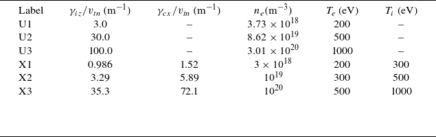
To test the applicability of (2.5), several cases are prepared with DEGAS2 using electron-impact ionisation as the only reaction included. For the purposes of estimating neutral density, this reaction is purely a sink precisely as it acts in (2.1), and DEGAS2 directly solves along trajectories by sampling the source distribution and dividing the domain into many sub-volumes to estimate neutral tallies. In these cases, the neutral thermal velocity corresponds to a temperature $T_n =$
100 eV. The electron density and temperature were chosen so that the three cases correspond to, within three significant figures,
$T_n =$
100 eV. The electron density and temperature were chosen so that the three cases correspond to, within three significant figures, $\hat {\gamma } = (3, 30, 100)$
, where
$\hat {\gamma } = (3, 30, 100)$
, where $\hat {\gamma } \equiv \gamma / v_{tn}$
is an inverse ‘mean free path’. This is a known to be an important quantity for fuelling (Fujii et al. Reference Fujii, Hasuo, Goto and Lore2025) and will remain dimensional with units of inverse length to stress that it does not directly scale with device size (Mordijck Reference Mordijck2020). Table 1 lists the properties of these test cases. Note that, by scanning in
$\hat {\gamma } \equiv \gamma / v_{tn}$
is an inverse ‘mean free path’. This is a known to be an important quantity for fuelling (Fujii et al. Reference Fujii, Hasuo, Goto and Lore2025) and will remain dimensional with units of inverse length to stress that it does not directly scale with device size (Mordijck Reference Mordijck2020). Table 1 lists the properties of these test cases. Note that, by scanning in $\hat {\gamma }$
, not only are different plasma conditions accounted for, but also different source thermal velocities.
$\hat {\gamma }$
, not only are different plasma conditions accounted for, but also different source thermal velocities.
List of the parameters used for the uniform-plasma cases considered here. Labels U1–U3 are the planar symmetry cases, and X1–X3 are the X-point cases. Also shown are the normalised rates for ionisation and charge exchange, respectively.

Predicted neutral density through a uniform-plasma domain with several normalised ionisation loss rates $ \hat {\gamma } = n_e \langle \sigma _{iz} v \rangle / v_{tn}$
and identical source rates. On the left (a) is a linear scale at low
$ \hat {\gamma } = n_e \langle \sigma _{iz} v \rangle / v_{tn}$
and identical source rates. On the left (a) is a linear scale at low $x$
, and on the right (b) is a logarithmic scale. The crosses are results from DEGAS2, the solid lines represent the numerical evaluation of the integral (2.2) and the dashed line is the analytic closed-form approximation (2.5). Cases correspond to those labelled U1, U2 and U3 in table 1.
$x$
, and on the right (b) is a logarithmic scale. The crosses are results from DEGAS2, the solid lines represent the numerical evaluation of the integral (2.2) and the dashed line is the analytic closed-form approximation (2.5). Cases correspond to those labelled U1, U2 and U3 in table 1.

Figure 2 shows these three cases comparing the DEGAS2 results with the model of (2.5). Also shown are the results from direct numerical calculation of the integral in (2.4). It is worth noting that all these cases have the same neutral source: a rate of $10^{22}$
particles per second per
$10^{22}$
particles per second per $\mathrm{m}^2$
and a source temperature of 100 eV. Agreement between the model and simulation is generally good, with some exceptions near
$\mathrm{m}^2$
and a source temperature of 100 eV. Agreement between the model and simulation is generally good, with some exceptions near $x=0$
. Since this is the foundation upon which more general models are built, it is worth examining the discrepancy. DEGAS2 utilises ‘suppressed ionisation’ whereby it directly uses the analytic solution of
$x=0$
. Since this is the foundation upon which more general models are built, it is worth examining the discrepancy. DEGAS2 utilises ‘suppressed ionisation’ whereby it directly uses the analytic solution of $f$
in (2.2), so it should, in principle, exactly match the direct numeric integration of (2.4). The reason any disagreement between DEGAS2 and numerical integration is seen at all in figure 2 is because DEGAS2 calculates a volume-averaged tally, whereas the function (2.2) is integrated at the particular values of
$f$
in (2.2), so it should, in principle, exactly match the direct numeric integration of (2.4). The reason any disagreement between DEGAS2 and numerical integration is seen at all in figure 2 is because DEGAS2 calculates a volume-averaged tally, whereas the function (2.2) is integrated at the particular values of $x$
. Since
$x$
. Since $n_n$
has a strong second derivative near
$n_n$
has a strong second derivative near $x=0$
, the volume-averaged density in a cell is slightly more than the value evaluated at the midpoint of the cell. A similar issue was encountered in the benchmarks of Bernard et al. (Reference Bernard, Halpern, Francisquez, Mandell, Juno, Hammett, Hakim, Wilkie and Guterl2022), requiring DEGAS2 to use higher resolution to capture higher-order variability within spatial cells. Additional disagreement is seen between the closed-form saddle point solution (2.5) and both the DEGAS2 results and direct integration of the kinetic equation. This disagreement is due to the breakdown of the saddle point approximation itself, wherein
$x=0$
, the volume-averaged density in a cell is slightly more than the value evaluated at the midpoint of the cell. A similar issue was encountered in the benchmarks of Bernard et al. (Reference Bernard, Halpern, Francisquez, Mandell, Juno, Hammett, Hakim, Wilkie and Guterl2022), requiring DEGAS2 to use higher resolution to capture higher-order variability within spatial cells. Additional disagreement is seen between the closed-form saddle point solution (2.5) and both the DEGAS2 results and direct integration of the kinetic equation. This disagreement is due to the breakdown of the saddle point approximation itself, wherein $\hat {\gamma }$
is not reliably considered asymptotically large, especially near
$\hat {\gamma }$
is not reliably considered asymptotically large, especially near $x=0$
. Even so, a disagreement of only
$x=0$
. Even so, a disagreement of only $\sim 25\,\%$
when the ‘large’ asymptotic parameter is much smaller than unity (approximately 0.03 for the
$\sim 25\,\%$
when the ‘large’ asymptotic parameter is much smaller than unity (approximately 0.03 for the $\hat {\gamma } = 3$
case at
$\hat {\gamma } = 3$
case at $x \approx 0.01$
) is remarkably fortunate. This might be an indication that the analytic approximation of (2.4), and those like it that follow, can be derived by other means.
$x \approx 0.01$
) is remarkably fortunate. This might be an indication that the analytic approximation of (2.4), and those like it that follow, can be derived by other means.
2.2. Pedestal loss with planar symmetry
The solution to (2.1) is readily found for any $\gamma (x)$
that admits a closed-form indefinite integral, but this work shall restrict itself to a particular functional form
$\gamma (x)$
that admits a closed-form indefinite integral, but this work shall restrict itself to a particular functional form
 \begin{equation} \gamma (x) = \gamma _0 + \frac {\gamma _\infty - \gamma _0}{2} \left [ 1 + \tanh \left (\frac {x-x_0}{\varDelta } \right ) \right ]\!, \end{equation}
where $x_0$
and
$x_0$
and $\varDelta$
are parameters defining the shape of
$\varDelta$
are parameters defining the shape of $\gamma (x)$
, while
$\gamma (x)$
, while $\gamma _0$
and
$\gamma _0$
and $\gamma _\infty$
are the left and right asymptotes of
$\gamma _\infty$
are the left and right asymptotes of $\gamma$
, corresponding to the SOL and core asymptotes, respectively. This form is inspired by the plasma profiles typically fit in the pedestal region of tokamaks (Groebner & Osborne Reference Groebner and Osborne1998). The interpretation of
$\gamma$
, corresponding to the SOL and core asymptotes, respectively. This form is inspired by the plasma profiles typically fit in the pedestal region of tokamaks (Groebner & Osborne Reference Groebner and Osborne1998). The interpretation of $\varDelta$
and
$\varDelta$
and $x_0$
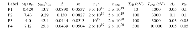
are the ‘pedestal’ half-width and the location of largest gradient, respectively. The loss profile shapes that will be used are listed in table 2. Note that the shapes and asymptotes of the internally fit loss-rate profile do not necessarily match that of the plasma itself, since the former is a tabulated function of the latter.
$x_0$
are the ‘pedestal’ half-width and the location of largest gradient, respectively. The loss profile shapes that will be used are listed in table 2. Note that the shapes and asymptotes of the internally fit loss-rate profile do not necessarily match that of the plasma itself, since the former is a tabulated function of the latter.
List of the parameters determining the loss-rate profiles tested for the spatially varying planar cases. Here, $\varDelta _e$
and
$\varDelta _e$
and $x_{0e}$
correspond to the pedestal shape properties of the electron population, where
$x_{0e}$
correspond to the pedestal shape properties of the electron population, where $\varDelta$
and
$\varDelta$
and $x_0$
are the parameters for the fitted shapes of the ionisation loss-rate profile
$x_0$
are the parameters for the fitted shapes of the ionisation loss-rate profile $\gamma (x)$
.
$\gamma (x)$
.

Under the functional form of (2.6), the solution to (2.1) is
 \begin{equation} f(x,v) = \frac {S(v)}{v} \exp \left ( \frac {x_0 - x}{v}\frac {\gamma _0 + \gamma _\infty }{2} \right ) \left \{ \frac { \cosh \left [{(x - x_0)}/{\varDelta } \right ]}{\cosh ({x_0}/{ \varDelta })} \right \}^{{\varDelta }/{v}\left ( \gamma _\infty - \gamma _0 \right )}. \end{equation}
The density moment under the same approximation as the previous section is
 \begin{equation} n_n(x) \approx \frac {2 S_0}{\sqrt {3 \pi }} \left ( \frac {u(x)}{2} \right )^{-1/3} \exp \left [- 3 \left ( \frac {u(x)}{2} \right )^{2/3}\right ]\!, \end{equation}
where
 \begin{equation} u(x) = \varDelta \frac {\gamma _\infty - \gamma _0}{2}\ln \left\{ \frac {\cosh \left [{(x -x_0)}/{\varDelta } \right ]}{ \cosh \left ({x_0}/{\varDelta } \right )}\right \} + \frac {\gamma _0+\gamma _\infty }{2}\left (x-x_0\right )\!. \end{equation}
With this model, the neutral density throughout a medium with a spatially varying loss rate can be estimated. Again, DEGAS2 is utilised for testing. Four artificial pedestals are constructed with the properties listed in table 2. In DEGAS2, electron density and temperature profiles are constructed similarly to (2.6). Then, the ionisation rate throughout the domain is fit to (2.6) to find the listed properties that determine $\hat {\gamma }(x)$
. The results from these simulations are shown in figure 3. Similar agreement is seen as for the uniform case: direct integration agrees better with the DEGAS2 than the model, especially at relatively low
$\hat {\gamma }(x)$
. The results from these simulations are shown in figure 3. Similar agreement is seen as for the uniform case: direct integration agrees better with the DEGAS2 than the model, especially at relatively low $\hat {\gamma }$
. Significant disagreement is seen for the ‘P1’ case at small
$\hat {\gamma }$
. Significant disagreement is seen for the ‘P1’ case at small $x$
since the ‘large’ asymptotic parameter is as low as
$x$
since the ‘large’ asymptotic parameter is as low as $5\times 10^{-3}$
. Agreement is recovered deeper into the domain as
$5\times 10^{-3}$
. Agreement is recovered deeper into the domain as $\hat {\gamma } x$
becomes larger.
$\hat {\gamma } x$
becomes larger.

3. Radial X-point source
In a diverted magnetic geometry, neutrals are present at significant densities near the divertor, which penetrate the separatrix most readily near the X-point, resulting in a poloidally localised fuelling. Reflection from the walls and interaction with the SOL plasma significantly complicates the picture and necessitates first-principles kinetic simulation for accurate fuelling profiles. In this section, the extreme case is considered of neutrals crossing the separatrix only at the X-point. The solution associated with this $\delta$
function source can in principle be extended as a Green’s function for a more general poloidal dependence of neutrals entering the domain from outside the separatrix.
$\delta$
function source can in principle be extended as a Green’s function for a more general poloidal dependence of neutrals entering the domain from outside the separatrix.
In this section, the geometry of the problem is adjusted to one of radial symmetry and a linear source of neutrals localised at the X-point (which subtends a circle of radius $R$
). See figure 1 for an illustration of the unstructured mesh for these cases.
$R$
). See figure 1 for an illustration of the unstructured mesh for these cases.
The source of neutrals is again an isotropic Maxwellian at 100 eV, nearly point-wise in the poloidal plane (actually, a very small volume adjacent to the X-point and subtended around the ‘tokamak’ axis of symmetry).
3.1. Uniform lossy plasma
In coordinates where $r$
is the distance to the X-point and
$r$
is the distance to the X-point and $v$
is the corresponding radial velocity, the kinetic equation is
$v$
is the corresponding radial velocity, the kinetic equation is
 \begin{equation} v \frac {\partial f}{\partial r} + \gamma f = \frac {S(v)}{2 \pi R} \frac {\delta (r)}{r}, \end{equation}
which admits the solution
 \begin{equation} f(r,v) = \frac {S(v)}{2 \pi R r v_{tn} } \frac {1}{v} e^{- \gamma r/v}. \end{equation}
With the now-familiar procedure of treating the source as Maxwellian and applying the saddle point method, the analytic model for neutral density is
 \begin{equation} n(r) \approx \frac {S_0}{\sqrt {12 \pi ^3} R v_{tn} r} \exp \left [ - 3 \left ( \frac {\gamma r}{2 v_{tn}} \right )^{2/3} \right ]\!. \end{equation}
In this geometry, the neutral density takes a slightly different form owing to the cancellation of the factor of $v$
due to the velocity integration measure
$v$
due to the velocity integration measure $\int [\ldots ]\,v\mathrm{d}v$
. This change is not inconsequential, as the solution more clearly departs from purely exponential behaviour (Fujii et al. Reference Fujii, Hasuo, Goto and Lore2025); see figure 4 for sample cases with three different pairs of uniform electron density and temperature (as listed in table 1).
$\int [\ldots ]\,v\mathrm{d}v$
. This change is not inconsequential, as the solution more clearly departs from purely exponential behaviour (Fujii et al. Reference Fujii, Hasuo, Goto and Lore2025); see figure 4 for sample cases with three different pairs of uniform electron density and temperature (as listed in table 1).
Comparing DEGAS2 simulation results with the closed-form model of (3.3) for three different uniform loss rates with a linear source. For visual clarity, different symbols: crosses and dots, are used to denote DEGAS2 results in the left-hand (linear scale) and right-hand (logarithmic scale) plots, respectively. Neutral density is plotted versus distance to the X-point for each volume element in the mesh. The three cases are listed as X1, X2 and X3 in table 1.

Note that the DEGAS2 results exhibit significant spread, with (3.3) capturing well the upper bound. The reason for this spread is a combination of: poloidal curvature of the lemniscate, toroidal curvature and finite extent of the numerical source. These effects are beyond the scope of the analytic model, but are worth noting and some aspects are discussed further in § 4.
Considering the spatial dependence of the neutral density from simulation, one can be easily imagine attributing the departure from exponential behaviour to charge exchange, but this reaction is not included in these cases. This is addressed in the following section.
3.2. Inclusion of charge exchange
In general, charge exchange involves the inclusion of a collision integral in the kinetic equation. However, it is often useful to approximate it as a relaxation operator (Wersal & Ricci Reference Wersal and Ricci2015; Bernard et al. Reference Bernard, Halpern, Francisquez, Mandell, Juno, Hammett, Hakim, Wilkie and Guterl2022) of the form $\gamma _{cx} \left[ (n/n_i) f_i - f \right]$
, where
$\gamma _{cx} \left[ (n/n_i) f_i - f \right]$
, where $f_i$
is a Maxwellian distribution of ions with density
$f_i$
is a Maxwellian distribution of ions with density $n_i$
and thermal velocity
$n_i$
and thermal velocity $v_{ti}$
. Effectively, this operator acts a sink of neutrals and replaces them with those sampled from the ion distribution
$v_{ti}$
. Effectively, this operator acts a sink of neutrals and replaces them with those sampled from the ion distribution $f_i$
. It is exact only if ion velocities are decoupled from those of neutrals: either through a particular (unphysical) form of the cross-section or by ion velocities being asymptotically large compared with neutrals (Wilkie et al. Reference Wilkie, Laggner, Hager, Rosenthal, Ku, Churchill, Horvath, Chang and Bortolon2024). Therefore, this operator does not act on velocity space rigorously. One can imagine the approximation
$f_i$
. It is exact only if ion velocities are decoupled from those of neutrals: either through a particular (unphysical) form of the cross-section or by ion velocities being asymptotically large compared with neutrals (Wilkie et al. Reference Wilkie, Laggner, Hager, Rosenthal, Ku, Churchill, Horvath, Chang and Bortolon2024). Therefore, this operator does not act on velocity space rigorously. One can imagine the approximation $v_{tn} \ll v_{ti}$
being valid, but it will not be formally applied here. The reason for not doing so is that neutrals penetrating the separatrix are likely to have already undergone a charge exchange reaction with a similar-temperature ion population outside the separatrix. If the neutral energy is very low compared with ions, they are not likely to have reached the separatrix in the first place.
$v_{tn} \ll v_{ti}$
being valid, but it will not be formally applied here. The reason for not doing so is that neutrals penetrating the separatrix are likely to have already undergone a charge exchange reaction with a similar-temperature ion population outside the separatrix. If the neutral energy is very low compared with ions, they are not likely to have reached the separatrix in the first place.
With the BGK form of the charge exchange operator, the kinetic equation (with a Maxwellian source) reads
 \begin{equation} v \frac {\partial f}{\partial r} + \left (\gamma _{iz} + \gamma _{cx} \right ) f = \frac {S_0}{2 \pi ^{2} R v_{tn}^2} e^{-v^2/v_{tn}^2} \frac {\delta (r)}{r} + \gamma _{cx} n(r) \frac {e^{-v^2/v_{ti}^2}}{\pi v_{ti}^2}. \end{equation}
The ion population is taken to be spatially uniform. Equation (3.4) introduces an additional complication: a source which depends on the undetermined neutral density. This remains tractable though by solving with a similar integrating factor
 \begin{align} f(r,v) &= \frac { S_0 }{2 \pi ^2 R v_{tn}^2 } \frac {1}{rv}\exp \left [ - \frac {v^2}{v_{tn}^2} - \frac {(\gamma _{iz} + \gamma _{cx})r}{v} \right ] \nonumber \\ &\quad + \frac {\gamma _{cx}}{\pi v_{ti}^2 v} \int \limits _0^r n(r') \exp \left [ -\frac {v^2}{v_{ti}^2} - \frac {\left ( \gamma _{iz} + \gamma _{cx} \right ) }{v} \left (r - r' \right )\right ] \, \mathrm{d}r'. \end{align}
Upon integrating over velocity (with the asymptotic solution of (3.3)), the result is
 \begin{equation} n(r) = n_0(r) + \frac {\gamma _{cx}}{\pi v_{ti}^2} \int \limits _0^r n(r') \int \exp \left [ -\frac {v^2}{v_{ti}^2} - \frac {\left ( \gamma _{iz} + \gamma _{cx} \right ) }{v} \left (r - r' \right )\right ] \, \mathrm{d}v\mathrm{d}r', \end{equation}
where
 \begin{equation} n_0(r) = \frac {S_0}{\sqrt {12 \pi ^3} R v_{tn} r} \exp \left \{ - 3 \left [ \frac { \left (\gamma _{iz} + \gamma _{cx} \right ) r}{ 2 v_{tn}} \right ]^{2/3} \right \}\!, \end{equation}
is a slightly modified version of (3.3) with $\gamma = \gamma _{iz} + \gamma _{cx}$
, treating the charge exchange rate as an additional loss. The form of (3.6) is a Fredholm integral equation of the second kind. Formally, this is solved with a Neumann series (Spanier & Gelbard Reference Spanier and Gelbard2008), and this is the formal foundation upon which the Monte Carlo method is based. This is effectively a series of successive application of the integral kernel to an iterated
$\gamma = \gamma _{iz} + \gamma _{cx}$
, treating the charge exchange rate as an additional loss. The form of (3.6) is a Fredholm integral equation of the second kind. Formally, this is solved with a Neumann series (Spanier & Gelbard Reference Spanier and Gelbard2008), and this is the formal foundation upon which the Monte Carlo method is based. This is effectively a series of successive application of the integral kernel to an iterated $n(r')$
, adding additional dimensionality to the integral at each iteration. A single such iteration is applied in this work, corresponding to neutrals undergoing only one charge exchange (‘first generation’). After applying the asymptotic expansion on the velocity integral and substituting
$n(r')$
, adding additional dimensionality to the integral at each iteration. A single such iteration is applied in this work, corresponding to neutrals undergoing only one charge exchange (‘first generation’). After applying the asymptotic expansion on the velocity integral and substituting $n_0(r')$
in the integrand
$n_0(r')$
in the integrand
 \begin{align} n(r) &\approx n_0(r) + \frac {\gamma _{cx} S_0}{\sqrt {12 \pi ^3} R v_{tn}^2 } \frac {T_n}{T_i} \left ( 1+ \frac {T_n}{T_i} \right )^{-1/6} \\ &\quad \times \left [ \frac { \left ( \gamma _{iz} + \gamma _{cx} \right ) r}{2 v_{tn}} \right ]^{-1/3} \exp \left \{ - 3 \left [ \frac { \left (\gamma _{iz} + \gamma _{cx} \right ) r}{ 2 v_{tn}} \right ]^{2/3} \left (1 + \frac {T_n}{T_i} \right )\right \}\!. \nonumber \end{align}
Once again, the model (3.8) is compared with results from DEGAS2 in figure 5 along with several other iterations for interpretation. These three cases are the same as in figure 4 (cases X1–X3 in table 1), but now with the charge exchange reaction included with ion populations at temperatures 300, 500 and 1000 eV, respectively. Several features of these cases are worthy of comment. Firstly, both the simulation results and model depart significantly from the case without charge exchange, so the effect is overall, as expected, non-trivial. Additionally, until the neutral density drops by nearly two orders of magnitude, both the model and the simulation are nearly indistinguishable from $n_0$
(3.7), which is labelled as the ‘Pure loss model’. This indicates that the effect of charge exchange near the X-point is primarily as a loss mechanism. Finally, for the most extreme case X3, there remains an order-unity departure of the simulation results from the model(s) at
$n_0$
(3.7), which is labelled as the ‘Pure loss model’. This indicates that the effect of charge exchange near the X-point is primarily as a loss mechanism. Finally, for the most extreme case X3, there remains an order-unity departure of the simulation results from the model(s) at $r \gtrsim 1\, \mathrm{cm}$
. There are three possible reasons for this discrepancy in terms of the physics included in DEGAS2, but not the analytic model: full collision operator and cross-section for charge exchange rather than the BGK form; neutrals are permitted to undergo more than one charge exchange interaction in the simulation; and speed of neutrals with respect to the at-rest ion population may not be well captured by
$r \gtrsim 1\, \mathrm{cm}$
. There are three possible reasons for this discrepancy in terms of the physics included in DEGAS2, but not the analytic model: full collision operator and cross-section for charge exchange rather than the BGK form; neutrals are permitted to undergo more than one charge exchange interaction in the simulation; and speed of neutrals with respect to the at-rest ion population may not be well captured by $v_{tn}$
.
$v_{tn}$
.
DEGAS2 results for neutral density throughout the mesh plotted versus distance of the centroid each element to the X-point (pale dots), compared with the analytic model of (3.8) for the three different uniform-plasma cases. Also shown (as dotted lines) are the cases without charge exchange and (dashed lines) the prediction of (3.7) with charge exchange treated purely as a loss. Plasma parameters correspond to those listed as X1, X2 and X3 in table 1.

The fact that charge exchange behaves as a loss near the X-point is evident from direct comparison of the simulation results in figure 6. There, it is evident that the neutral penetration is decreased when charge exchange is included. This is due to the geometry of the problem. After a charge exchange event, the resulting neutral is sampled from the ion Maxwellian distribution. Most – approximately 75 % – of the post-charge exchange neutrals will therefore be on a trajectory that leaves the domain rather than penetrating deeper toward the core.
Examples (corresponding to case X1) of neutral density from DEGAS2 when ion charge exchange is ignored (left) or included (right).

The lossy behaviour of charge exchange observed here is not universal. In fact, the energy of the source neutrals is driven largely by the charge exchange reaction outside the separatrix, manifesting as a larger $v_{tn}$
and a lower effective loss rate
$v_{tn}$
and a lower effective loss rate $\hat {\gamma } = \gamma / v_{tn}$
.
$\hat {\gamma } = \gamma / v_{tn}$
.
4. Discussion and conclusion
The progression of models presented in previous sections provides an analytic framework whereby penetration of neutrals within the separatrix can be transparently understood. Complications in various permutations were considered: planar versus linear source geometry, spatial variation of the plasma and the inclusion of the BGK form of the charge exchange operator.
The mean-free path, $\hat {\gamma }^{-1} = v_{tn}/\gamma$
, remains an important parameter. However, since higher energy neutrals penetrate deeper than those of low energy, the neutral density does not decrease with a simple exponential even in a uniformly ionising domain. Instead, forms such as (2.4) and (3.3) are more appropriate for general use and interpretation of spatially resolved neutral diagnostics (once multiplied by the local emission rate).
$\hat {\gamma }^{-1} = v_{tn}/\gamma$
, remains an important parameter. However, since higher energy neutrals penetrate deeper than those of low energy, the neutral density does not decrease with a simple exponential even in a uniformly ionising domain. Instead, forms such as (2.4) and (3.3) are more appropriate for general use and interpretation of spatially resolved neutral diagnostics (once multiplied by the local emission rate).
For the linear X-point source models, it was found that charge exchange acts primarily as a loss. Second-generation effects do appear inside the separatrix, but only sufficiently far from the X-point after the neutral density drops orders of magnitude. Additional results consistently reveal that treating charge exchange as a pure loss based primarily on reaction rates at the X-point is rather accurate when compared with more complete equivalent-source simulations, even in the presence of a plasma transport barrier. The reason is because of flux expansion: near the X-point, the gradient of a flux function ( $\psi$
) is small. So even if, for example,
$\psi$
) is small. So even if, for example, $n_e'(\psi )$
is very high, this does not necessarily translate to a very large
$n_e'(\psi )$
is very high, this does not necessarily translate to a very large $|\boldsymbol{\nabla }n_e|$
. Especially in cases where the neutral penetration depth is small, the plasma relevant for neutral interaction is effectively uniform in the vicinity of the X-point. This, coupled with the observation that the role of charge exchange is primarily as a loss mechanism, means that the relatively simple model of (3.3) performs better than expected, even though it does not include a charge exchange reaction as such, nor does it allow for spatially varying plasma. These additional complications can readily be included in a closed-form, albeit more complicated, model.
$|\boldsymbol{\nabla }n_e|$
. Especially in cases where the neutral penetration depth is small, the plasma relevant for neutral interaction is effectively uniform in the vicinity of the X-point. This, coupled with the observation that the role of charge exchange is primarily as a loss mechanism, means that the relatively simple model of (3.3) performs better than expected, even though it does not include a charge exchange reaction as such, nor does it allow for spatially varying plasma. These additional complications can readily be included in a closed-form, albeit more complicated, model.
The model and analysis presented here open up additional routes of inquiry. Primarily, how ought the neutral source near the X-point be characterised in terms of their velocity and spatial distribution? How can the isotropic Maxwellian source be improved? To what extent does the model need to be adapted to account for neutrals re-entering the domain after charge exchange in the SOL? Answering these questions will require follow-up study of the neutral transport outside of the confined plasma: in the SOL, divertor and private flux regions.
One can imagine using the model in the form of (2.8) or (3.3) as a fitting function for neutral profiles observed experimentally. While developing the model further along these lines is encouraged, the reader is nevertheless urged to caution until and unless the spatial and velocity distribution of neutrals is properly accounted for. Throughout the preparation of this work, it was easy to fit nearly any neutral profile observed in simulation to a function like (2.8). Once such a function is fit to data, the physical relevance of the loss rate, the spatial or velocity distribution of the neutral source or the role of the spatial coordinate $r$
can all be misinterpreted if one is not careful.
$r$
can all be misinterpreted if one is not careful.
Throughout this analysis, the open magnetic field region has been excluded entirely. Instead, the neutral source was modelled as an isotropic Maxwellian at a given temperature. While $T_n =$
100 eV was used universally throughout this work, sufficient generality was nevertheless included (with respect to testing the model) via a range of values of
$T_n =$
100 eV was used universally throughout this work, sufficient generality was nevertheless included (with respect to testing the model) via a range of values of $\hat {\gamma }$
– loss rate normalised to an inverse length via the neutral thermal speed. Similarly, device size (particularly major radius
$\hat {\gamma }$
– loss rate normalised to an inverse length via the neutral thermal speed. Similarly, device size (particularly major radius $R$
) appears in a prefactor on the source rate, making the neutral density profile proportional to the number of source particles per length around the circumference of the magnetic null.
$R$
) appears in a prefactor on the source rate, making the neutral density profile proportional to the number of source particles per length around the circumference of the magnetic null.
The X-point fuelling source presented here is just that: point-wise in the poloidal plane. Considering the very strong drop-off of the neutral density (e.g. within $r \lt 1\,\mathrm{mm}$
in figure 4
a), a more general spatial distribution of neutrals is expected to significantly impact the results. Fortunately, the model source is a Dirac delta, so that the model itself can act as a Green’s function for follow-up work once the neutral spatial distribution incoming from the divertor is more properly characterised. Beyond the spatial distribution of neutrals, the isotropic Maxwellian source developed upon here is likely also insufficient. Indeed, any sensitivity to the normalised reaction rate
$r \lt 1\,\mathrm{mm}$
in figure 4
a), a more general spatial distribution of neutrals is expected to significantly impact the results. Fortunately, the model source is a Dirac delta, so that the model itself can act as a Green’s function for follow-up work once the neutral spatial distribution incoming from the divertor is more properly characterised. Beyond the spatial distribution of neutrals, the isotropic Maxwellian source developed upon here is likely also insufficient. Indeed, any sensitivity to the normalised reaction rate $\hat {\gamma }$
is implicitly a sensitivity study to the neutral source velocity distribution. Modifications such as a cosine velocity angle distribution or Poisson energy distribution can be readily incorporated, but further study outside the scope of this work is required whether for general or device-specific models. These results do, however, isolate the key characteristics needed for such a study: the neutral velocity distribution near the X-point, and the spatial distribution of the incoming flux.
$\hat {\gamma }$
is implicitly a sensitivity study to the neutral source velocity distribution. Modifications such as a cosine velocity angle distribution or Poisson energy distribution can be readily incorporated, but further study outside the scope of this work is required whether for general or device-specific models. These results do, however, isolate the key characteristics needed for such a study: the neutral velocity distribution near the X-point, and the spatial distribution of the incoming flux.
Acknowledgements
The author is grateful to S. Haskey, Q. Pratt, S. Newton, A. Bortolon and F. Parra for fruitful discussions.
Editor Troy Carter thanks the referees for their advice in evaluating this article.
Funding
This work was supported by the U.S. Department of Energy through under contract number DE-AC02-09CH11466 and the SciDAC project ‘Computational Evaluation and Design of Actuators for Core-Edge Integration’ (CEDA). The United States Government retains a non-exclusive, paid-up, irrevocable, world-wide licence to publish or reproduce the published form of this manuscript, or allow others to do so, for United States Government purposes.
Declaration of interests
The author reports no conflict of interest.


 Open access