





1. Introduction
One of the central questions in wall-bounded turbulence concerns the scaling of mean and fluctuating velocities with wall distance and Reynolds number. In the classical framework (Prandtl Reference Prandtl1925), the relevant velocity scale is the friction velocity, $ u_{\tau } = ( {\tau _w}/{\rho } )^{1/2},$
where
$ u_{\tau } = ( {\tau _w}/{\rho } )^{1/2},$
where $\tau _w$
is the wall shear stress and
$\tau _w$
is the wall shear stress and $\rho$
the fluid density. The friction velocity is directly linked to the pressure gradient required to sustain the flow, particularly in pipe flow, which is the primary focus of this study. Two characteristic length scales naturally arise: the viscous inner length
$\rho$
the fluid density. The friction velocity is directly linked to the pressure gradient required to sustain the flow, particularly in pipe flow, which is the primary focus of this study. Two characteristic length scales naturally arise: the viscous inner length $\delta _v = \nu / u_{\tau }$
, with
$\delta _v = \nu / u_{\tau }$
, with $\nu$
the kinematic viscosity, and the inertial outer length
$\nu$
the kinematic viscosity, and the inertial outer length $\delta$
, associated with the overall dimensions of the wall layer and taken as
$\delta$
, associated with the overall dimensions of the wall layer and taken as $\delta = R$
, where
$\delta = R$
, where $R$
is the pipe radius, for pipe flow. The present work focuses specifically on modelling the variance of the streamwise velocity in turbulent pipe flow, a canonical configuration for the study of wall-bounded shear turbulence.
$R$
is the pipe radius, for pipe flow. The present work focuses specifically on modelling the variance of the streamwise velocity in turbulent pipe flow, a canonical configuration for the study of wall-bounded shear turbulence.
1.1. Logarithmic layer
Modelling of velocity variances in wall-bounded turbulence dates back to the 1950s, and efforts were initially focused on the overlap layer (or logarithmic layer), where the mean velocity shows an approximate logarithmic wall-normal dependence (von Kármán Reference von Kármán1931). From this observation, Townsend (Reference Townsend1956, Reference Townsend1976) set out a theoretical framework, where the variance of velocity is modelled as a superposition of second-order statistical moments of energy-containing eddies ‘attached to the wall’; i.e. the attached-eddy model (AEM). The AEM assumes that each of the attached eddies is statistically self-similar with respect to the distance from their core to the wall (attached-eddy hypothesis; AEH). Townsend subsequently introduced a generic form of second-order statistical moments of individual energy-containing attached eddies, under the assumption that they would behave ‘inviscidly’ in the logarithmic layer. In doing so, a slip boundary condition is applied to the wall-parallel velocity components, while the no-penetration condition is enforced on the wall-normal velocity on the wall. One of the key predictions of the model is that, in order to retain the asymptotically uniform turbulent shear stress expected from the mean equation in the logarithmic layer, the wall-parallel velocity variances must exhibit a logarithmic decay with respect to the outer-scaled wall distance.
Several important refinements of Townsend’s original theory were later introduced, these include: (i) the description of the logarithmic mean velocity in terms of the mean vorticity of individual attached eddies (Perry & Chong Reference Perry and Chong1982; Perry, Henbest & Chong Reference Perry, Henbest and Chong1986); (ii) the prescription of a more realistic statistical form for the individual attached eddy (Perry & Chong Reference Perry and Chong1982; Perry et al. Reference Perry, Henbest and Chong1986; Woodcock & Marusic Reference Woodcock and Marusic2015); (iii) the connection between the physical-space model of Townsend and the $k^{-1}$
behaviour of velocity spectra (where
$k^{-1}$
behaviour of velocity spectra (where $k$
is the wall-parallel wavenumber) (Perry & Chong Reference Perry and Chong1982; Perry et al. Reference Perry, Henbest and Chong1986); (iv) empirical extensions toward the near-wall region (Marusic & Kunkel Reference Marusic and Kunkel2003); and (v) the generalisation of the Townsend–Perry logarithmic law to higher-order turbulence statistics (Meneveau & Marusic Reference Meneveau and Marusic2013). Furthermore, there has been a substantial amount of theoretical, numerical and experimental evidence supporting the existence of self-similar wall-attached energy-containing eddies throughout the logarithmic layer. The AEH itself has recently been theoretically proven using the spectral energy budget of the Navier–Stokes equations (Hwang & Lee Reference Hwang and Lee2020), and there has been substantial evidence for the existence of self-similar energy-containing eddies (e.g. Tomkins & Adrian Reference Tomkins and Adrian2003; del Álamo et al. Reference del Álamo, Jiménez, Zandonade and Moser2006; Hwang Reference Hwang2015; Hellström et al. Reference Hellström, Marusic and Smits2016; Hwang & Sung Reference Hwang and Sung2018; Baars & Marusic Reference Baars and Marusic2020a
, and many others), with the supporting modelling and analysis of the Navier–Stokes equations (Hwang & Cossu Reference Hwang and Cossu2010; Klewicki Reference Klewicki2013; Moarref et al. Reference Moarref, Sharma, Tropp and McKeon2013; Eckhardt & Zammert Reference Eckhardt and Zammert2018; Yang, Willis & Hwang Reference Yang, Willis and Hwang2019; Azimi & Schneider Reference Azimi and Schneider2020; Hwang & Eckhardt Reference Hwang and Eckhardt2020; Hwang & Lee Reference Hwang and Lee2020).
$k$
is the wall-parallel wavenumber) (Perry & Chong Reference Perry and Chong1982; Perry et al. Reference Perry, Henbest and Chong1986); (iv) empirical extensions toward the near-wall region (Marusic & Kunkel Reference Marusic and Kunkel2003); and (v) the generalisation of the Townsend–Perry logarithmic law to higher-order turbulence statistics (Meneveau & Marusic Reference Meneveau and Marusic2013). Furthermore, there has been a substantial amount of theoretical, numerical and experimental evidence supporting the existence of self-similar wall-attached energy-containing eddies throughout the logarithmic layer. The AEH itself has recently been theoretically proven using the spectral energy budget of the Navier–Stokes equations (Hwang & Lee Reference Hwang and Lee2020), and there has been substantial evidence for the existence of self-similar energy-containing eddies (e.g. Tomkins & Adrian Reference Tomkins and Adrian2003; del Álamo et al. Reference del Álamo, Jiménez, Zandonade and Moser2006; Hwang Reference Hwang2015; Hellström et al. Reference Hellström, Marusic and Smits2016; Hwang & Sung Reference Hwang and Sung2018; Baars & Marusic Reference Baars and Marusic2020a
, and many others), with the supporting modelling and analysis of the Navier–Stokes equations (Hwang & Cossu Reference Hwang and Cossu2010; Klewicki Reference Klewicki2013; Moarref et al. Reference Moarref, Sharma, Tropp and McKeon2013; Eckhardt & Zammert Reference Eckhardt and Zammert2018; Yang, Willis & Hwang Reference Yang, Willis and Hwang2019; Azimi & Schneider Reference Azimi and Schneider2020; Hwang & Eckhardt Reference Hwang and Eckhardt2020; Hwang & Lee Reference Hwang and Lee2020).
Despite the progress made on AEH in recent decades, the predictions of the AEM modelling framework remain rather unsatisfactory, and this is primarily due to viscous effects not considered in the classical theories of Townsend and Perry (Hwang, Hutchins & Marusic Reference Hwang, Hutchins and Marusic2022). Early experimental measurements in pipe flow found that the $k^{-1}$
spectra, predicted by Perry et al. (Reference Perry, Henbest and Chong1986), do not emerge convincingly in the logarithmic layer (Morrison et al. Reference Morrison, Jiang, McKeon and Smits2001, Reference Morrison, McKeon, Jiang and Smits2004; Rosenberg et al. Reference Rosenberg, Hultmark, Vallikivi, Bailey and Smits2013; Vallikivi, Ganapathisubramani & Smits Reference Vallikivi, Ganapathisubramani and Smits2015). An outer peak in the spectra was found there instead (Morrison et al. Reference Morrison, McKeon, Jiang and Smits2004; Hutchins & Marusic Reference Hutchins and Marusic2007). As the friction Reynolds number,
$k^{-1}$
spectra, predicted by Perry et al. (Reference Perry, Henbest and Chong1986), do not emerge convincingly in the logarithmic layer (Morrison et al. Reference Morrison, Jiang, McKeon and Smits2001, Reference Morrison, McKeon, Jiang and Smits2004; Rosenberg et al. Reference Rosenberg, Hultmark, Vallikivi, Bailey and Smits2013; Vallikivi, Ganapathisubramani & Smits Reference Vallikivi, Ganapathisubramani and Smits2015). An outer peak in the spectra was found there instead (Morrison et al. Reference Morrison, McKeon, Jiang and Smits2004; Hutchins & Marusic Reference Hutchins and Marusic2007). As the friction Reynolds number, $\textit{Re}_\tau (=u_{\tau } \delta / \nu )$
, increases, the spectral intensity of this peak has been found to grow, while the corresponding (streamwise) wavelength and the wall-normal location slowly decrease (Mathis, Hutchins & Marusic Reference Mathis, Hutchins and Marusic2009; Vallikivi et al. Reference Vallikivi, Ganapathisubramani and Smits2015). In contrast, the logarithmic dependence in the wall-normal direction, predicted by Townsend (Reference Townsend1956), has been consistently observed to be a reliable first approximation for the streamwise and spanwise velocity variances at least for
$\textit{Re}_\tau (=u_{\tau } \delta / \nu )$
, increases, the spectral intensity of this peak has been found to grow, while the corresponding (streamwise) wavelength and the wall-normal location slowly decrease (Mathis, Hutchins & Marusic Reference Mathis, Hutchins and Marusic2009; Vallikivi et al. Reference Vallikivi, Ganapathisubramani and Smits2015). In contrast, the logarithmic dependence in the wall-normal direction, predicted by Townsend (Reference Townsend1956), has been consistently observed to be a reliable first approximation for the streamwise and spanwise velocity variances at least for $\textit{Re}_\tau \gtrsim O(10^3)$
(Jiménez & Hoyas Reference Jiménez and Hoyas2008; Hultmark et al. Reference Hultmark, Vallikivi, Bailey and Smits2012; Hultmark et al. Reference Hultmark, Vallikivi, Bailey and Smits2013; Marusic et al. Reference Marusic, Monty, Hultmark and Smits2013). The modelling effort of Baars & Marusic (Reference Baars and Marusic2020a
) with their experimental data suggests that a well-visible
$\textit{Re}_\tau \gtrsim O(10^3)$
(Jiménez & Hoyas Reference Jiménez and Hoyas2008; Hultmark et al. Reference Hultmark, Vallikivi, Bailey and Smits2012; Hultmark et al. Reference Hultmark, Vallikivi, Bailey and Smits2013; Marusic et al. Reference Marusic, Monty, Hultmark and Smits2013). The modelling effort of Baars & Marusic (Reference Baars and Marusic2020a
) with their experimental data suggests that a well-visible $k^{-1}$
spectrum may appear for
$k^{-1}$
spectrum may appear for $\textit{Re}_\tau \gtrsim 8\times 10^4$
. The disparity between the simulation/measurement data at relatively low
$\textit{Re}_\tau \gtrsim 8\times 10^4$
. The disparity between the simulation/measurement data at relatively low $\textit{Re}_\tau$
and the theory of Perry et al. (Reference Perry, Henbest and Chong1986) was recently addressed by Hwang et al. (Reference Hwang, Hutchins and Marusic2022), who showed that a well-developed
$\textit{Re}_\tau$
and the theory of Perry et al. (Reference Perry, Henbest and Chong1986) was recently addressed by Hwang et al. (Reference Hwang, Hutchins and Marusic2022), who showed that a well-developed $k^{-1}$
spectrum is not a necessary condition for an approximately logarithmic wall-normal dependence of the velocity variance observed, with the derivation of a weak
$k^{-1}$
spectrum is not a necessary condition for an approximately logarithmic wall-normal dependence of the velocity variance observed, with the derivation of a weak $\textit{Re}_\tau$
dependence of the Townsend–Perry constant. They also extended Townsend’s classical result to the mesolayer (i.e. the lower part of the logarithmic layer) by introducing an empirical model for the viscous effect on the spectra. Apart from the AEM framework, it is finally worth mentioning the recent work of Chen & Sreenivasan (Reference Chen and Sreenivasan2023), who proposed a different form of variance for streamwise/spanwise velocity and pressure, based on their bounded-dissipation framework (Chen & Sreenivasan Reference Chen and Sreenivasan2021, see also below for a further discussion).
$\textit{Re}_\tau$
dependence of the Townsend–Perry constant. They also extended Townsend’s classical result to the mesolayer (i.e. the lower part of the logarithmic layer) by introducing an empirical model for the viscous effect on the spectra. Apart from the AEM framework, it is finally worth mentioning the recent work of Chen & Sreenivasan (Reference Chen and Sreenivasan2023), who proposed a different form of variance for streamwise/spanwise velocity and pressure, based on their bounded-dissipation framework (Chen & Sreenivasan Reference Chen and Sreenivasan2021, see also below for a further discussion).
1.2. Near-wall region
Studies on velocity variances in the near-wall region are relatively recent compared with those in the logarithmic layer. Early studies suggested that, within the inner layer where viscous effects remain significant, both mean velocity and velocity variances would be universal when expressed in wall units ( $u_{\tau }$
and
$u_{\tau }$
and $\delta _v$
) (e.g. Sreenivasan Reference Sreenivasan1989; Mochizuki & Nieuwstadt Reference Mochizuki and Nieuwstadt1996). This view is well supported for the mean velocity, but experimental and numerical data (Spalart Reference Spalart1988; DeGraaff & Eaton Reference DeGraaff and Eaton2000; Metzger & Klewicki Reference Metzger and Klewicki2001; Marusic & Kunkel Reference Marusic and Kunkel2003, among others) have shown that streamwise velocity variances near the wall exhibit a pronounced Reynolds-number dependence. Foremost among them is the extended AEM formulation for the near-wall region (Marusic & Kunkel Reference Marusic and Kunkel2003), which predicts that streamwise velocity variances should increase logarithmically with
$\delta _v$
) (e.g. Sreenivasan Reference Sreenivasan1989; Mochizuki & Nieuwstadt Reference Mochizuki and Nieuwstadt1996). This view is well supported for the mean velocity, but experimental and numerical data (Spalart Reference Spalart1988; DeGraaff & Eaton Reference DeGraaff and Eaton2000; Metzger & Klewicki Reference Metzger and Klewicki2001; Marusic & Kunkel Reference Marusic and Kunkel2003, among others) have shown that streamwise velocity variances near the wall exhibit a pronounced Reynolds-number dependence. Foremost among them is the extended AEM formulation for the near-wall region (Marusic & Kunkel Reference Marusic and Kunkel2003), which predicts that streamwise velocity variances should increase logarithmically with $ \textit{Re}_{\tau }$
at any fixed
$ \textit{Re}_{\tau }$
at any fixed $y^+=y/\delta _v$
, consistent with the experimental measurement and numerical simulation data available at that time.
$y^+=y/\delta _v$
, consistent with the experimental measurement and numerical simulation data available at that time.
About a decade later, a different view from Marusic & Kunkel (Reference Marusic and Kunkel2003) was proposed by Monkewitz & Nagib (Reference Monkewitz and Nagib2015), who combined an asymptotic analysis of the mean equation in turbulent boundary layers with direct numerical simulation (DNS) data available at higher Reynolds numbers. In particular, their analysis suggests that the streamwise velocity variance near the wall may be bounded as $\textit{Re}_\tau \rightarrow \infty$
and that its growth with
$\textit{Re}_\tau \rightarrow \infty$
and that its growth with $\textit{Re}_\tau$
is inversely proportional to
$\textit{Re}_\tau$
is inversely proportional to $\log \textit{Re}_\tau$
(or the free stream mean velocity
$\log \textit{Re}_\tau$
(or the free stream mean velocity $U_\infty$
in the boundary layer, equivalently). Although experimental measurements near the wall remain not fully conclusive due to the different facilities and measurement techniques used, emerging DNS data appear to support the notion that the streamwise velocity variance near the wall may be bounded as
$U_\infty$
in the boundary layer, equivalently). Although experimental measurements near the wall remain not fully conclusive due to the different facilities and measurement techniques used, emerging DNS data appear to support the notion that the streamwise velocity variance near the wall may be bounded as $\textit{Re}_\tau \rightarrow \infty$
(Chen & Sreenivasan Reference Chen and Sreenivasan2021; Hwang Reference Hwang2024; Pirozzoli Reference Pirozzoli2024). From this observation, Chen & Sreenivasan (Reference Chen and Sreenivasan2021) proposed a defect power law, where the streamwise velocity variance near the wall is proportional to
$\textit{Re}_\tau \rightarrow \infty$
(Chen & Sreenivasan Reference Chen and Sreenivasan2021; Hwang Reference Hwang2024; Pirozzoli Reference Pirozzoli2024). From this observation, Chen & Sreenivasan (Reference Chen and Sreenivasan2021) proposed a defect power law, where the streamwise velocity variance near the wall is proportional to $\textit{Re}_\tau ^{-1/4}$
, with a hypothesis that the streamwise wall dissipation is bounded by the maximum possible production of near-wall turbulence. By analysing near-wall spectra from DNS and experiment, Hwang (Reference Hwang2024) showed that the boundedness of the streamwise velocity variance near the wall is due to viscous effects that gradually limit the near-wall influence of large energy-containing eddies on increasing
$\textit{Re}_\tau ^{-1/4}$
, with a hypothesis that the streamwise wall dissipation is bounded by the maximum possible production of near-wall turbulence. By analysing near-wall spectra from DNS and experiment, Hwang (Reference Hwang2024) showed that the boundedness of the streamwise velocity variance near the wall is due to viscous effects that gradually limit the near-wall influence of large energy-containing eddies on increasing $\textit{Re}_\tau$
. Furthermore, by extending the spectral AEM of Perry et al. (Reference Perry, Henbest and Chong1986) to the near-wall region, they proposed that, if the streamwise velocity variance near the wall is bounded, it would be inversely proportional to
$\textit{Re}_\tau$
. Furthermore, by extending the spectral AEM of Perry et al. (Reference Perry, Henbest and Chong1986) to the near-wall region, they proposed that, if the streamwise velocity variance near the wall is bounded, it would be inversely proportional to $\log \textit{Re}_\tau$
.
$\log \textit{Re}_\tau$
.
The recent work by Pirozzoli (Reference Pirozzoli2024) went a step further from Hwang (Reference Hwang2024) by introducing a physical model for the near-wall influence of large energy-containing eddies and constructing formulas to extrapolate finite-Reynolds-number DNS results to arbitrarily high $ \textit{Re}_{\tau }$
. Their analysis of spanwise spectra in the viscous near-wall region provided evidence for the existence of an overlap between inner- and outer-scaled spectral ranges, characterised by a
$ \textit{Re}_{\tau }$
. Their analysis of spanwise spectra in the viscous near-wall region provided evidence for the existence of an overlap between inner- and outer-scaled spectral ranges, characterised by a $k^{-1+\alpha }$
scaling, which is shallower than that predicted by the classical AEM. This behaviour reflects the progressive attenuation of the influence of large energy-containing eddies on the near-wall region as viscous effects become important, and thus quantifies the deviation of the spectra from the
$k^{-1+\alpha }$
scaling, which is shallower than that predicted by the classical AEM. This behaviour reflects the progressive attenuation of the influence of large energy-containing eddies on the near-wall region as viscous effects become important, and thus quantifies the deviation of the spectra from the $k^{-1}$
behaviour expected from the AEM. As a consequence, the contribution of the largest scales of motion to the streamwise velocity variance was found to decrease slowly with Reynolds number, leading to a defect power law of the form
$k^{-1}$
behaviour expected from the AEM. As a consequence, the contribution of the largest scales of motion to the streamwise velocity variance was found to decrease slowly with Reynolds number, leading to a defect power law of the form $\langle u^2 \rangle ^+ = A - B \, \textit{Re}_{\tau }^{-\alpha }$
, with
$\langle u^2 \rangle ^+ = A - B \, \textit{Re}_{\tau }^{-\alpha }$
, with $\alpha \approx 0.18$
inferred from DNS data. In the absence of such effects (
$\alpha \approx 0.18$
inferred from DNS data. In the absence of such effects ( $\alpha =0$
), the classical
$\alpha =0$
), the classical $\log \textit{Re}_\tau$
scaling of the AEM is recovered.
$\log \textit{Re}_\tau$
scaling of the AEM is recovered.
1.3. Scope
Regardless of the physical models, predicting the distribution of turbulent stresses at a given Reynolds number remains a major challenge. While the logarithmic law of the wall for the mean velocity profile is now well established, and semi-empirical models exist for the complete velocity distribution in both boundary layers and internal flows (Musker Reference Musker1979), the situation is far less consolidated for quantities such as the streamwise velocity variance. Existing models are often based on classical inviscid theories (Marusic & Kunkel Reference Marusic and Kunkel2003; Baars & Marusic Reference Baars and Marusic2020b
), or on limited viscous corrections thereof (Hwang et al. Reference Hwang, Hutchins and Marusic2022), and they struggle to provide accurate predictions of the velocity variance across the entire wall-normal domain. From a different standpoint, recent modelling efforts within the bounded-dissipation framework (Chen & Sreenivasan Reference Chen and Sreenivasan2021, Reference Chen and Sreenivasan2023; Monkewitz Reference Monkewitz2022) rely on one-point turbulence statistics, which are difficult to link with their two-point counterparts that have been well characterised through the statistical and dynamical analysis of coherent structures over the past two decades. Other attempts include the work of Alfredsson, Segalini & Örlü (Reference Alfredsson, Segalini and Örlü2011), who showed that, over a wide Reynolds-number range, the turbulence intensity in the outer layer follows a linear empirical relation with the local mean velocity, which implies that an outer peak must emerge once sufficient scale separation is achieved. Their analysis further predicts that the position of this outer peak scales approximately as $ \textit{Re}_{\tau }^{0.56}$
and that its amplitude increases logarithmically with Reynolds number.
$ \textit{Re}_{\tau }^{0.56}$
and that its amplitude increases logarithmically with Reynolds number.
The first key goal of this paper is to assess and model streamwise velocity (azimuthal wavenumber) spectra in turbulent pipe flow. The focus will be on the region in and below the lower logarithmic layer, where viscous effects on energy-containing eddies are significant. In particular, we will combine the physical model of Bradshaw (Reference Bradshaw1967) for inactive motions (i.e. the wall-attached, Reynolds-shear-stress-free component of the energy-containing eddies) with the spectral scaling identified by Pirozzoli (Reference Pirozzoli2024). We will then develop an alternative model for the spectral region where $k^{-1}$
behaviour is expected to emerge, according to the classical inviscid formulation of Perry et al. (Reference Perry, Henbest and Chong1986). Achieving this goal will be instrumental in establishing scaling laws for the streamwise velocity variance, obtained by integration in spectral space. To guide the discussion, it is useful to anticipate the spectral framework employed throughout the paper. The velocity spectra are interpreted by partitioning spectral space into four regions associated with distinct physical mechanisms: (i) a small-scale viscous range dominated by the buffer-layer dynamics; (ii) an intermediate range corresponding to the near-wall footprint of wall-attached eddies; (iii) an outer part of the attached-eddy range representing their off-wall influence; and (iv) a large-scale outer region associated with motions scaling with the pipe radius. Each region is modelled separately, and their integrated contributions are combined to predict the wall-normal distribution of the streamwise velocity variance. Ultimately, the objective is to derive a complete and explicit representation of the streamwise velocity variance, including its Reynolds-number dependence and its extrapolation to values well beyond those currently accessible. We also compare the present model with the classical formulation of Perry et al. (Reference Perry, Henbest and Chong1986), as well as with the recently proposed coherent-structure-based model of Gustenyov, Bayley & Smits (Reference Gustenyov, Bayley and Smits2025). The latter reproduces the Reynolds-number evolution of the streamwise velocity variance by superposing spectral contributions from different coherent motions, whereas the present approach derives the variance distribution by integrating region-specific spectral scalings inferred from DNS data.
$k^{-1}$
behaviour is expected to emerge, according to the classical inviscid formulation of Perry et al. (Reference Perry, Henbest and Chong1986). Achieving this goal will be instrumental in establishing scaling laws for the streamwise velocity variance, obtained by integration in spectral space. To guide the discussion, it is useful to anticipate the spectral framework employed throughout the paper. The velocity spectra are interpreted by partitioning spectral space into four regions associated with distinct physical mechanisms: (i) a small-scale viscous range dominated by the buffer-layer dynamics; (ii) an intermediate range corresponding to the near-wall footprint of wall-attached eddies; (iii) an outer part of the attached-eddy range representing their off-wall influence; and (iv) a large-scale outer region associated with motions scaling with the pipe radius. Each region is modelled separately, and their integrated contributions are combined to predict the wall-normal distribution of the streamwise velocity variance. Ultimately, the objective is to derive a complete and explicit representation of the streamwise velocity variance, including its Reynolds-number dependence and its extrapolation to values well beyond those currently accessible. We also compare the present model with the classical formulation of Perry et al. (Reference Perry, Henbest and Chong1986), as well as with the recently proposed coherent-structure-based model of Gustenyov, Bayley & Smits (Reference Gustenyov, Bayley and Smits2025). The latter reproduces the Reynolds-number evolution of the streamwise velocity variance by superposing spectral contributions from different coherent motions, whereas the present approach derives the variance distribution by integrating region-specific spectral scalings inferred from DNS data.
2. The DNS database
We utilise the DNS database compiled by Pirozzoli (Reference Pirozzoli2024), which includes simulations up to $ \textit{Re}_{\tau } \approx 12{\,}000$
. Table 1 lists the flow cases, with details on the computational mesh and key parameters. The numerical algorithm follows the formulation of Pirozzoli et al. (Reference Pirozzoli, Romero, Fatica, Verzicco and Orlandi2021), with particular attention to grid resolution and box-size effects, as discussed in Pirozzoli (Reference Pirozzoli2024). As shown in table 1, the largest simulations span fewer than ten eddy turnover times, a standard threshold for statistical convergence (Hoyas & Jiménez Reference Hoyas and Jiménez2006). A more stringent assessment based on the method of Russo & Luchini (Reference Russo and Luchini2017) indicates that the standard deviation in the prediction of streamwise velocity variance, up to the edge of the logarithmic layer, does not exceed
$ \textit{Re}_{\tau } \approx 12{\,}000$
. Table 1 lists the flow cases, with details on the computational mesh and key parameters. The numerical algorithm follows the formulation of Pirozzoli et al. (Reference Pirozzoli, Romero, Fatica, Verzicco and Orlandi2021), with particular attention to grid resolution and box-size effects, as discussed in Pirozzoli (Reference Pirozzoli2024). As shown in table 1, the largest simulations span fewer than ten eddy turnover times, a standard threshold for statistical convergence (Hoyas & Jiménez Reference Hoyas and Jiménez2006). A more stringent assessment based on the method of Russo & Luchini (Reference Russo and Luchini2017) indicates that the standard deviation in the prediction of streamwise velocity variance, up to the edge of the logarithmic layer, does not exceed $0.6\,\%$
. Uncertainty is naturally larger in the velocity spectra, for which confidence bands were provided and analysed in detail by Pirozzoli (Reference Pirozzoli2024).
$0.6\,\%$
. Uncertainty is naturally larger in the velocity spectra, for which confidence bands were provided and analysed in detail by Pirozzoli (Reference Pirozzoli2024).
Flow parameters for the DNS of turbulent pipe flow. Here, $R$
is the pipe radius;
$R$
is the pipe radius; $L_z$
the pipe axial length;
$L_z$
the pipe axial length; $N_{\theta }$
,
$N_{\theta }$
, $N_r$
and
$N_r$
and $N_z$
the number of grid points in the azimuthal, radial and axial directions, respectively;
$N_z$
the number of grid points in the azimuthal, radial and axial directions, respectively; $ \textit{Re}_b = 2 R u_b / \nu$
is the bulk Reynolds number;
$ \textit{Re}_b = 2 R u_b / \nu$
is the bulk Reynolds number; $f = 8 \tau _w / (\rho u_b^2)$
the friction factor;
$f = 8 \tau _w / (\rho u_b^2)$
the friction factor; $ \textit{Re}_{\tau } = u_{\tau } R / \nu$
the friction Reynolds number;
$ \textit{Re}_{\tau } = u_{\tau } R / \nu$
the friction Reynolds number; $T$
the sampling time used to collect flow statistics; and
$T$
the sampling time used to collect flow statistics; and $\tau _t = R / u_{\tau }$
the eddy turnover time.
$\tau _t = R / u_{\tau }$
the eddy turnover time.

Table 1. Long description
The table lists flow parameters for turbulent pipe flow simulations. It includes seven rows and nine columns. The columns are labeled as follows: Flow case, L z slash R, Mesh (N theta times N r times N z), Re b, f, Re tau, T slash T l, and Line style. The row labels are flow cases B, C, D, E, F, and G. Each row provides specific values for the parameters. For example, Row 1: Flow case B, L z slash R 15, Mesh 768 times 96 times 768, Re b 17000, f 0.02719, Re tau 495.6, T slash T l 192.9, Line style green. Row 2: Flow case C, L z slash R 15, Mesh 1792 times 164 times 1792, Re b 44000, f 0.02119, Re tau 1132.2, T slash T l 50.4, Line style cyan. Row 3: Flow case D, L z slash R 15, Mesh 3072 times 243 times 3072, Re b 82500, f 0.01828, Re tau 1972.0, T slash T l 45.1, Line style yellow. Row 4: Flow case E, L z slash R 15, Mesh 4608 times 327 times 4608, Re b 133000, f 0.01657, Re tau 3026.8, T slash T l 26.9, Line style orange. Row 5: Flow case F, L z slash R 15, Mesh 9216 times 546 times 9216, Re b 285000, f 0.01421, Re tau 6006.4, T slash T l 18.2, Line style magenta. Row 6: Flow case G, L z slash R 15, Mesh 18432 times 1024 times 18432, Re b 612000, f 0.01242, Re tau 12054.5, T slash T l 6.99, Line style black.
3. Questions
Mean velocity profiles (a) and streamwise velocity variance profiles (b) for turbulent pipe flow at various Reynolds numbers (see table 1 for colour codes).

A central question in studies of wall turbulence concerns the difference between the mean velocity profiles and the streamwise velocity variance profiles, shown in figure 1. The figure highlights the universality of the mean velocity profiles when expressed in wall units. As the Reynolds number increases, the main effect is the progressive extension of the logarithmic layer to higher $y^+$
. In contrast, the streamwise velocity variance (panel b) exhibits marked non-universality, with values increasing at any fixed
$y^+$
. In contrast, the streamwise velocity variance (panel b) exhibits marked non-universality, with values increasing at any fixed $y^+$
. This behaviour, long recognised in the literature but still difficult to quantify experimentally, represents a major theoretical challenge in wall turbulence, as it signals a clear departure from strictly local wall scaling.
$y^+$
. This behaviour, long recognised in the literature but still difficult to quantify experimentally, represents a major theoretical challenge in wall turbulence, as it signals a clear departure from strictly local wall scaling.
The lack of universality of $\langle u^{2} \rangle$
can be interpreted by examining the spectral maps shown in figure 2, which display the spanwise spectral density of the streamwise velocity fluctuations (
$\langle u^{2} \rangle$
can be interpreted by examining the spectral maps shown in figure 2, which display the spanwise spectral density of the streamwise velocity fluctuations ( $E_{uu}$
) in pre-multiplied form,
$E_{uu}$
) in pre-multiplied form, $k_{\theta } E_{uu}$
, where
$k_{\theta } E_{uu}$
, where $k_{\theta}=2 \pi / \lambda_{\theta}$
is the wavenumber in the azimuthal direction. This representation is frequently used because equal areas under the curve correspond to equal contributions to the variance, and because it has the dimensions of a squared velocity. Hence,
$k_{\theta}=2 \pi / \lambda_{\theta}$
is the wavenumber in the azimuthal direction. This representation is frequently used because equal areas under the curve correspond to equal contributions to the variance, and because it has the dimensions of a squared velocity. Hence, $k_{\theta } E_{uu}$
can be effectively interpreted as providing the wall-normal distribution of the kinetic energy associated with eddies of a given size. Two Reynolds numbers are shown for comparison. As is well established, the spectral maps exhibit two primary energetic sites: an inner site scaling with
$k_{\theta } E_{uu}$
can be effectively interpreted as providing the wall-normal distribution of the kinetic energy associated with eddies of a given size. Two Reynolds numbers are shown for comparison. As is well established, the spectral maps exhibit two primary energetic sites: an inner site scaling with $\delta _v$
, and an outer site scaling with
$\delta _v$
, and an outer site scaling with $R$
. Between these two regions, a diagonal ridge of energetic modes is observed, corresponding to Townsend’s attached eddies. The figure also reveals an additional energetic band connecting the inner and outer sites along the line
$R$
. Between these two regions, a diagonal ridge of energetic modes is observed, corresponding to Townsend’s attached eddies. The figure also reveals an additional energetic band connecting the inner and outer sites along the line $y = \beta \lambda_{\theta}$
(with
$y = \beta \lambda_{\theta}$
(with $\beta \approx 0.11$
), which can be tentatively interpreted as the signature of wall-attached eddies. Wall-parallel velocity fluctuations are relatively unaffected by the presence of the wall, hence the near-wall imprint of the attached eddies is rather strong. As a consequence, the streamwise velocity variance – obtained by integrating the velocity auto-spectrum over wavenumber space – is highly non-uniform and shows pronounced Reynolds-number sensitivity, due to the increasing energy contribution from larger eddies at fixed
$\beta \approx 0.11$
), which can be tentatively interpreted as the signature of wall-attached eddies. Wall-parallel velocity fluctuations are relatively unaffected by the presence of the wall, hence the near-wall imprint of the attached eddies is rather strong. As a consequence, the streamwise velocity variance – obtained by integrating the velocity auto-spectrum over wavenumber space – is highly non-uniform and shows pronounced Reynolds-number sensitivity, due to the increasing energy contribution from larger eddies at fixed $y^+$
. Since the streamwise velocity variance is obtained by integrating the spectral density over wavenumber space, the wall-normal behaviour of
$y^+$
. Since the streamwise velocity variance is obtained by integrating the spectral density over wavenumber space, the wall-normal behaviour of $\langle u^2 \rangle$
can be interpreted as the cumulative contribution of eddies of different sizes. Consequently, identifying the dominant spectral regions and their scaling behaviour provides a direct route to modelling its wall-normal distribution. Figure 2 reveals a similar morphology of the spectral maps across Reynolds numbers. At the same time, it shows that, for any fixed
$\langle u^2 \rangle$
can be interpreted as the cumulative contribution of eddies of different sizes. Consequently, identifying the dominant spectral regions and their scaling behaviour provides a direct route to modelling its wall-normal distribution. Figure 2 reveals a similar morphology of the spectral maps across Reynolds numbers. At the same time, it shows that, for any fixed $y^+$
location in the near-wall region, an increasing range of large wavelengths associated with outer-scaled motions extends down to the wall. This behaviour underlies the lack of universality observed in figure 1(b). The objective of this paper is therefore to quantify this non-universality and to develop predictive models for the evolution of the streamwise velocity variance with
$y^+$
location in the near-wall region, an increasing range of large wavelengths associated with outer-scaled motions extends down to the wall. This behaviour underlies the lack of universality observed in figure 1(b). The objective of this paper is therefore to quantify this non-universality and to develop predictive models for the evolution of the streamwise velocity variance with $y^+$
and
$y^+$
and $ \textit{Re}_{\tau }$
, grounded in physical reasoning and guided by DNS data.
$ \textit{Re}_{\tau }$
, grounded in physical reasoning and guided by DNS data.
4. Analysis
Spectral maps for flow case F (panel (a), $ \textit{Re}_{\tau } \approx 6{\,}000$
) and flow case G (panel (b),
$ \textit{Re}_{\tau } \approx 6{\,}000$
) and flow case G (panel (b), $ \textit{Re}_{\tau } \approx 12{\,}000$
) with an overlaid conceptual sketch of the four regions considered in the analysis. Iso-contours of
$ \textit{Re}_{\tau } \approx 12{\,}000$
) with an overlaid conceptual sketch of the four regions considered in the analysis. Iso-contours of $k^+_{\theta } E^+_{uu}$
are shown from
$k^+_{\theta } E^+_{uu}$
are shown from $0.36$
to
$0.36$
to $3.6$
, at intervals of
$3.6$
, at intervals of $0.36$
. The bounds of the small and large scales,
$0.36$
. The bounds of the small and large scales, $\lambda _S$
and
$\lambda _S$
and $\lambda _{\ell }$
, are marked by vertical lines, whose intersections with the main energetic diagonal ridge define
$\lambda _{\ell }$
, are marked by vertical lines, whose intersections with the main energetic diagonal ridge define $y_s$
and
$y_s$
and $y_{\ell }$
, respectively. The dashed diagonal red line denotes the bound of the dissipative range in the logarithmic layer, as given in (A2).
$y_{\ell }$
, respectively. The dashed diagonal red line denotes the bound of the dissipative range in the logarithmic layer, as given in (A2).

The strategy adopted here is to construct simplified models for the spectral density in different portions of the spectral map and to evaluate their contributions to the velocity variance separately. The subdivision into regions is guided by the dominant physical mechanisms in each part of spectral space, as well as by the scaling trends observed in the DNS data. The key idea underlying this analysis is illustrated in figure 2. Taking inspiration from Hwang (Reference Hwang2024), we tentatively subdivide the $\lambda$
axis into three sub-regions, corresponding to small, intermediate and large scales. Region I corresponds to the small scales, defined as those smaller than a fixed multiple of the viscous length scale (here,
$\lambda$
axis into three sub-regions, corresponding to small, intermediate and large scales. Region I corresponds to the small scales, defined as those smaller than a fixed multiple of the viscous length scale (here, $\lambda ^{+} \leqslant \lambda _s^{+} = 400$
). An obvious counterargument is that the so-called ‘small’ scales (interpreted as dissipative scales) vary with wall distance. For instance, it is known that in the logarithmic layer the Kolmogorov scale increases approximately as
$\lambda ^{+} \leqslant \lambda _s^{+} = 400$
). An obvious counterargument is that the so-called ‘small’ scales (interpreted as dissipative scales) vary with wall distance. For instance, it is known that in the logarithmic layer the Kolmogorov scale increases approximately as ${y^{+}}^{1/4}$
(Jiménez Reference Jiménez2012). However, this increase is sufficiently gradual that it produces no inconsistencies in the present analysis, as demonstrated in the following sections. Region IV corresponds to the large scales, defined as those larger than a fixed fraction of the outer length scale (here,
${y^{+}}^{1/4}$
(Jiménez Reference Jiménez2012). However, this increase is sufficiently gradual that it produces no inconsistencies in the present analysis, as demonstrated in the following sections. Region IV corresponds to the large scales, defined as those larger than a fixed fraction of the outer length scale (here, $\lambda \geqslant \lambda _{\ell } = 0.5 R$
). The intermediate range lies between these two limits, and widens with increasing
$\lambda \geqslant \lambda _{\ell } = 0.5 R$
). The intermediate range lies between these two limits, and widens with increasing $ \textit{Re}_{\tau }$
. We further subdivide this intermediate range – associated primarily with wall-attached eddies according to the AEM – into two parts: region II, beneath the primary energetic ridge, representing the near-wall footprint of attached eddies; and region III, above the ridge, corresponding to their influence farther from the wall. Associated with this splitting are two relevant off-wall locations, which correspond to the intersection of the diagonal line
$ \textit{Re}_{\tau }$
. We further subdivide this intermediate range – associated primarily with wall-attached eddies according to the AEM – into two parts: region II, beneath the primary energetic ridge, representing the near-wall footprint of attached eddies; and region III, above the ridge, corresponding to their influence farther from the wall. Associated with this splitting are two relevant off-wall locations, which correspond to the intersection of the diagonal line $y = \beta \lambda$
with the vertical line
$y = \beta \lambda$
with the vertical line $\lambda = \lambda _s$
, which results in
$\lambda = \lambda _s$
, which results in $y^+_s = 44$
; and with the vertical line
$y^+_s = 44$
; and with the vertical line $\lambda = \lambda _{\ell }$
, which results in
$\lambda = \lambda _{\ell }$
, which results in $y_{\ell }/R = 0.055$
.
$y_{\ell }/R = 0.055$
.
As a first step, we construct suitable spectral models for each of these regions, also with the goal of combining them into a unified predictive model for the wall-normal distribution of the velocity variance.
4.1. Spectra in region II
This region plays a crucial role in wall turbulence, as it corresponds to the near-wall footprint of wall-attached eddies. According to Bradshaw (Reference Bradshaw1967) and Townsend (Reference Townsend1976), the effect of ‘distant’ wall-attached eddies on the near-wall region is mainly a low-frequency modulation of the wall shear stress, to which the local turbulence can readjust quasi-instantaneously, so that the law of the wall holds locally in time. Under this assumption, the resulting velocity fluctuations have a variance that can be expressed as
 \begin{equation} \langle u^2 \rangle ^{+} \sim \left (U^{+} + y^{+} \frac {\mathrm{d} U^{+}}{\mathrm{d} y^{+}}\right )^2 \equiv F(y^{+}) . \end{equation}
The key implication of this argument is that the spectral density associated with the footprint of attached eddies varies with wall distance only through the modulation function $F(y^+)$
. Hence, once the spectral distribution is known at a reference location, its variation with
$F(y^+)$
. Hence, once the spectral distribution is known at a reference location, its variation with $y^+$
can be predicted by simple rescaling. This ansatz has been partially validated in previous studies (Jiménez Reference Jiménez2024; Pirozzoli Reference Pirozzoli2024). Assuming that the same relation applies to the spectral energy density of eddies with sizes
$y^+$
can be predicted by simple rescaling. This ansatz has been partially validated in previous studies (Jiménez Reference Jiménez2024; Pirozzoli Reference Pirozzoli2024). Assuming that the same relation applies to the spectral energy density of eddies with sizes $\lambda _{s} \leqslant \lambda \leqslant \lambda _{\ell }$
, the spectral density at any
$\lambda _{s} \leqslant \lambda \leqslant \lambda _{\ell }$
, the spectral density at any $y^{+}$
can be predicted once it is known at a reference wall distance
$y^{+}$
can be predicted once it is known at a reference wall distance $y_{0}^{+}$
, namely
$y_{0}^{+}$
, namely
 \begin{equation} (k^{+} E_{u}^{+})(\lambda ^{+},y^{+}) = (k^{+} E_{u}^{+})(\lambda ^{+},y_{0}^{+}) \frac {F(y^{+})}{F(y_{0}^{+})} . \end{equation}
Pre-multiplied $u$
spectrum for flow case G (a) and reconstructed spectrum based on (4.2) (b). Iso-contours of
$u$
spectrum for flow case G (a) and reconstructed spectrum based on (4.2) (b). Iso-contours of $k^+_{\theta } E^+_{uu}$
are shown from
$k^+_{\theta } E^+_{uu}$
are shown from $0.36$
to
$0.36$
to $3.6$
, at intervals of
$3.6$
, at intervals of $0.36$
. The dashed horizontal line in panel (b) marks the reference location used for the reconstruction (
$0.36$
. The dashed horizontal line in panel (b) marks the reference location used for the reconstruction ( $y_0^{+} = 15$
).
$y_0^{+} = 15$
).

Figure 3. Long description
Two contour plots depict the pre-multiplied spectrum and reconstructed spectrum for flow case G. Panel A shows the pre-multiplied spectrum with iso-contours of a variable ranging from 10^-4 to 10^0 at intervals of 10^0.2. The x-axis is labeled lambda theta plus, and the y-axis is labeled y plus. Panel B shows the reconstructed spectrum based on equation 4.2, with the same iso-contours and axis labels. A dashed horizontal line in Panel B marks the reference location used for the reconstruction at y plus equals 100.
Equation (4.2) is tested in figure 3, where the original spectral map (a) is compared with the reconstructed map, obtained by extrapolating the spectral density from the centre of the buffer layer ( $y_0^{+} = 15$
, b). The figure shows remarkable agreement not only within region II, but throughout the entire region beneath the primary energetic ridge. This confirms the physical validity of assumption (4.2) and demonstrates that the near-wall region of wall-bounded flows can be largely interpreted in terms of ‘turbulent Stokes layers’, namely local turbulent boundary layers whose dynamics is controlled by the overlying eddies. In our view, this represents a central result in wall-turbulence theory, with significant implications for the subsequent analysis.
$y_0^{+} = 15$
, b). The figure shows remarkable agreement not only within region II, but throughout the entire region beneath the primary energetic ridge. This confirms the physical validity of assumption (4.2) and demonstrates that the near-wall region of wall-bounded flows can be largely interpreted in terms of ‘turbulent Stokes layers’, namely local turbulent boundary layers whose dynamics is controlled by the overlying eddies. In our view, this represents a central result in wall-turbulence theory, with significant implications for the subsequent analysis.
Pre-multiplied spectra of $u$
at
$u$
at $y_0^{+} = 15$
. See table 1 for colour codes.
$y_0^{+} = 15$
. See table 1 for colour codes.

Whereas (4.2) predicts accurately the variation of the spectral density with wall-normal distance, a complete description also requires determining its dependence on wavelength at the reference position $y_0^{+}$
. The analysis reported by Pirozzoli (Reference Pirozzoli2024) addresses this very point. As shown in figure 4, the pre-multiplied spectral density at fixed
$y_0^{+}$
. The analysis reported by Pirozzoli (Reference Pirozzoli2024) addresses this very point. As shown in figure 4, the pre-multiplied spectral density at fixed $y^{+}$
exhibits an intermediate (overlap) range with a clear power-law behaviour
$y^{+}$
exhibits an intermediate (overlap) range with a clear power-law behaviour
 \begin{equation} (k^{+} E_{u}^{+})(\lambda ^{+},y_{0}^{+}) = A \, \left ( \lambda ^{+} \right )^{-\alpha } , \end{equation}
with $\alpha = 0.18$
and
$\alpha = 0.18$
and $A = 3.37$
at
$A = 3.37$
at $y_{0}^{+} = 15$
. It is worth noting that (4.3) slightly (but decisively) departs from the classical theory of Perry & Chong (Reference Perry and Chong1982), which would suggest
$y_{0}^{+} = 15$
. It is worth noting that (4.3) slightly (but decisively) departs from the classical theory of Perry & Chong (Reference Perry and Chong1982), which would suggest $\alpha =0$
. Combining equations (4.3) and (4.2) yields a complete theoretical prediction for the spectrum in region II.
$\alpha =0$
. Combining equations (4.3) and (4.2) yields a complete theoretical prediction for the spectrum in region II.
Evaluation of the velocity variance in region II involves integrating the spectrum (4.2) over the appropriate wavelength range. Referring to figure 2 for guidance, for $y^+ \leqslant y_s^+$
one obtains
$y^+ \leqslant y_s^+$
one obtains
 \begin{equation} \lt u^2\gt ^+_{\textit{II}} (y^+) = \int _{\log \lambda _s^+}^{\log \lambda _{\ell }^+} k_{\theta }^+ E_u^+ \, \mathrm{d} \log \lambda _{\theta }^+ \approx \frac {A F(y^+)}{\alpha F(15)} \left [ \left (\lambda _s^+\right )^{-\alpha }-\left (\frac {\lambda _{\ell }}R\right )^{-\alpha } \textit{Re}_{\tau }^{-\alpha } \right ] \!; \end{equation}
whereas for $y_s^+ \leqslant y^+ \leqslant y_{\ell }^+$
one has
$y_s^+ \leqslant y^+ \leqslant y_{\ell }^+$
one has
 \begin{align} \lt u^2\gt ^+_{\textit{II}} (y^+) = \int _{\log (y^+/\beta )}^{\log \lambda _{\ell }^+} k_{\theta }^+ E_u^+ \, \mathrm{d} \log \lambda _{\theta }^+ \approx \frac {A F(y^+)}{\alpha F(15)} \left [ \left (\frac {y^+}{\beta }\right )^{-\alpha }-\left (\frac {\lambda _{\ell }}R\right )^{-\alpha } \textit{Re}_{\tau }^{-\alpha } \right ] \!. \end{align}
Streamwise velocity variance for region II. The DNS data are shown as solid lines; dashed lines correspond to the prediction of (4.4), and dash-dotted lines to (4.5). Vertical lines indicate the characteristic off-wall locations $y_s^{+}$
and
$y_s^{+}$
and $y_{\ell }^{+}$
(the latter for flow case G). See table 1 for colour codes.
$y_{\ell }^{+}$
(the latter for flow case G). See table 1 for colour codes.

These two formulas are tested in figure 5. The solid lines represent the velocity variance from region II extracted from the DNS data, the dashed lines correspond to the predictive (4.4) and the dot–dashed line to (4.5). The figure demonstrates good predictive capability of the present analysis, although the accuracy of (4.5) is slightly reduced, particularly just beyond the kink at the upper end of the distributions. Despite minor discrepancies in the shape, the results confirm the strong predictive performance of the present theory with respect to variations in Reynolds number – an even more significant outcome, as it indicates that the energetic contribution of the intermediate eddies can be confidently extrapolated beyond the currently accessible Reynolds-number range.
4.2. Spectra in region III
Pre-multiplied spectral density of $u$
in region III for flow case G. Data are shown at five wall distances (listed in the figure inset) and plotted as a function of either
$u$
in region III for flow case G. Data are shown at five wall distances (listed in the figure inset) and plotted as a function of either $\lambda ^+$
(a) and of the similarity variable
$\lambda ^+$
(a) and of the similarity variable $\zeta = \beta \lambda / y$
(b). The grey line in (b) refers to the fitting function defined in (4.6).
$\zeta = \beta \lambda / y$
(b). The grey line in (b) refers to the fitting function defined in (4.6).

The spectra in region III are seldom analysed in detail. In the AEM framework, this region, located at the top left of the main energetic ridge, can be associated with two mechanisms: (i) the influence of wall-attached eddies on points located farther from the wall (local in $\lambda$
, non-local in
$\lambda$
, non-local in $y$
); and (ii) the energy cascade of wall-attached eddies toward smaller scales (local in
$y$
); and (ii) the energy cascade of wall-attached eddies toward smaller scales (local in $y$
, non-local in
$y$
, non-local in $\lambda$
). This region is likely unaffected by direct viscous effects, as well as by indirect effects associated with wall proximity. Possible viscous effects are nevertheless discussed in Appendix A. Hence, dimensional analysis suggests that the spectral density of
$\lambda$
). This region is likely unaffected by direct viscous effects, as well as by indirect effects associated with wall proximity. Possible viscous effects are nevertheless discussed in Appendix A. Hence, dimensional analysis suggests that the spectral density of $u$
depends only on the ratio
$u$
depends only on the ratio $\lambda / y$
, rather than on
$\lambda / y$
, rather than on $\lambda$
and
$\lambda$
and $y$
separately, as originally argued by Perry & Chong (Reference Perry and Chong1982). Strong support for this assumption can also be drawn from experimental data (e.g. Baars & Marusic Reference Baars and Marusic2020a
). Geometrical evidence for this universal behaviour is provided in figure 2, which shows that in this region the iso-lines of the pre-multiplied spectral density are aligned along diagonal bands. This behaviour is confirmed more quantitatively in figure 6, where we report the pre-multiplied spectral density at five off-wall distances in the logarithmic layer for the flow case G. When shown as a function of
$y$
separately, as originally argued by Perry & Chong (Reference Perry and Chong1982). Strong support for this assumption can also be drawn from experimental data (e.g. Baars & Marusic Reference Baars and Marusic2020a
). Geometrical evidence for this universal behaviour is provided in figure 2, which shows that in this region the iso-lines of the pre-multiplied spectral density are aligned along diagonal bands. This behaviour is confirmed more quantitatively in figure 6, where we report the pre-multiplied spectral density at five off-wall distances in the logarithmic layer for the flow case G. When shown as a function of $\lambda ^{+}$
(panel a), no universality is observed. However, the data clearly indicate the formation of two subranges with distinct power-law behaviour: a
$\lambda ^{+}$
(panel a), no universality is observed. However, the data clearly indicate the formation of two subranges with distinct power-law behaviour: a $(\lambda ^{+})^{2/3}$
scaling at smaller wavelengths and a
$(\lambda ^{+})^{2/3}$
scaling at smaller wavelengths and a $(\lambda ^{+})^{1}$
scaling at larger wavelengths. The former corresponds to an underlying
$(\lambda ^{+})^{1}$
scaling at larger wavelengths. The former corresponds to an underlying $E_u^{+} \sim (k^{+})^{-5/3}$
Kolmogorov inertial behaviour, and therefore becomes apparent only at sufficiently large
$E_u^{+} \sim (k^{+})^{-5/3}$
Kolmogorov inertial behaviour, and therefore becomes apparent only at sufficiently large $y^{+}$
, as expected under the assumption of a local energy cascade at fixed
$y^{+}$
, as expected under the assumption of a local energy cascade at fixed $y^+$
. The latter corresponds to a pre-multiplied spectrum behaving as
$y^+$
. The latter corresponds to a pre-multiplied spectrum behaving as $E_u^{+} \sim (k^{+})^{-2}$
. To the best of our knowledge, this scaling has not been clearly reported in previous experimental studies, although it can also be identified in spectra from DNS of turbulent channel flow (Lee & Moser Reference Lee and Moser2015) (not shown here). Possible explanations for the emergence of this ‘odd’ scaling may be related to the prevalence of sharp interfaces, ramps and quasi-two-dimensional shear layers in the logarithmic region (Meinhart & Adrian Reference Meinhart and Adrian1995; de Silva, Hutchins & Marusic Reference de Silva, Hutchins and Marusic2016), whose likely spectral footprint is a
$E_u^{+} \sim (k^{+})^{-2}$
. To the best of our knowledge, this scaling has not been clearly reported in previous experimental studies, although it can also be identified in spectra from DNS of turbulent channel flow (Lee & Moser Reference Lee and Moser2015) (not shown here). Possible explanations for the emergence of this ‘odd’ scaling may be related to the prevalence of sharp interfaces, ramps and quasi-two-dimensional shear layers in the logarithmic region (Meinhart & Adrian Reference Meinhart and Adrian1995; de Silva, Hutchins & Marusic Reference de Silva, Hutchins and Marusic2016), whose likely spectral footprint is a $k^{-2}$
velocity spectrum (Pullin & Saffman Reference Pullin and Saffman1998). This interpretation likely deserves a dedicated follow-up study; however, the observed trend appears robust for the present purposes.
$k^{-2}$
velocity spectrum (Pullin & Saffman Reference Pullin and Saffman1998). This interpretation likely deserves a dedicated follow-up study; however, the observed trend appears robust for the present purposes.
The same data are reported in figure 6(b) as a function of the similarity variable $\zeta = \beta \lambda / y$
, such that
$\zeta = \beta \lambda / y$
, such that $\zeta = 1$
corresponds to the main energetic ridge in figure 2. Points with
$\zeta = 1$
corresponds to the main energetic ridge in figure 2. Points with $\zeta \gt 1$
belong to region II and are therefore omitted from the present analysis. In this representation, a clear near universality of the spectra emerges at intermediate values of
$\zeta \gt 1$
belong to region II and are therefore omitted from the present analysis. In this representation, a clear near universality of the spectra emerges at intermediate values of $\zeta$
. Deviations are observed at small
$\zeta$
. Deviations are observed at small $\zeta$
, where the dissipative range begins to influence the spectrum. Some scatter is also observed as
$\zeta$
, where the dissipative range begins to influence the spectrum. Some scatter is also observed as $\zeta \to 1$
, where the energy is found to increase slightly with
$\zeta \to 1$
, where the energy is found to increase slightly with $y^{+}$
, consistent with the trends reported by Jiménez (Reference Jiménez2024) and with those identified in our analysis for region II. For the sole purpose of deriving an analytical prediction for the contribution of this region to the velocity variance, we fit the pre-multiplied spectra using a simple polynomial function
$y^{+}$
, consistent with the trends reported by Jiménez (Reference Jiménez2024) and with those identified in our analysis for region II. For the sole purpose of deriving an analytical prediction for the contribution of this region to the velocity variance, we fit the pre-multiplied spectra using a simple polynomial function
 \begin{equation} p(\zeta ) = A \left [ \zeta + (3 q - 2) \, \zeta ^{2} + (1 - 2 q) \, \zeta ^{3} \right ]\!, \end{equation}
which reproduces the observed $E_u^{+} \sim (k^{+})^{-2}$
scaling at small
$E_u^{+} \sim (k^{+})^{-2}$
scaling at small $\zeta$
and has zero derivative at
$\zeta$
and has zero derivative at $\zeta = 1$
, where the spectral density attains a peak. The fitting parameters determined from the DNS data are
$\zeta = 1$
, where the spectral density attains a peak. The fitting parameters determined from the DNS data are $A = 4.8$
and
$A = 4.8$
and $q = 1/3$
. We note that this function does not reproduce the
$q = 1/3$
. We note that this function does not reproduce the $E_u^{+} \sim (k^{+})^{-5/3}$
dissipative spectral range observed in figure 6(b) at small wavelengths. However, the contribution of the latter to the velocity variance is small, as shown in Appendix A, so that the resulting error in the modelled velocity variance is negligible.
$E_u^{+} \sim (k^{+})^{-5/3}$
dissipative spectral range observed in figure 6(b) at small wavelengths. However, the contribution of the latter to the velocity variance is small, as shown in Appendix A, so that the resulting error in the modelled velocity variance is negligible.
Streamwise velocity variance for region III. The DNS data are shown as solid lines; dashed lines correspond to the prediction of (4.7), and dash-dotted lines to (4.9). Vertical lines indicate the characteristic off-wall locations $y_s^{+}$
and
$y_s^{+}$
and $y_{\ell }^{+}$
(the latter for flow case G). See table 1 for colour codes.
$y_{\ell }^{+}$
(the latter for flow case G). See table 1 for colour codes.

Integration of the model spectrum (4.6) yields the contribution to the streamwise velocity variance from region III. As in region II, referring to figure 2, we must distinguish two sub-cases. For $y_s^+ \leqslant y^+ \leqslant y_{\ell }^+$
, integration gives
$y_s^+ \leqslant y^+ \leqslant y_{\ell }^+$
, integration gives
 \begin{equation} \overline {u^2}^+_{\textit{III}} (y^+) = \int _{\log \lambda _{s}^+}^{\log (y^+/\beta )} k_{\theta }^+ E_u^+ \, \mathrm{d} \log \lambda _{\theta }^+ \approx \int _{\beta \lambda _s^+ / y^+}^1 \frac {p(\zeta )}{\zeta } \, \mathrm{d} \zeta = P(1) - P(\beta \lambda _s^+ / y^+), \end{equation}
with
 \begin{equation} P(\zeta ) = A \left [ \zeta + (3 q - 2) \frac {\zeta ^2}2 + (1-2 q) \frac {\zeta ^3}3 \right ]\!; \end{equation}
whereas for $y^+ \geqslant y_{\ell }^+$
it yields
$y^+ \geqslant y_{\ell }^+$
it yields
 \begin{align} \overline {u^2}^+_{\textit{III}} (y^+) = \int _{\log \lambda _s^+}^{\log \lambda _{\ell }^+} k_{\theta }^+ E_u^+ \, \mathrm{d} \log \lambda _{\theta }^+ \approx \int _{\beta \lambda _s^+ / y}^{\beta \lambda _{\ell }^+ / y^+} \frac {p(\zeta )}{\zeta } \, \mathrm{d} \zeta = P(\beta \lambda _{\ell }^+ / y^+) - P(\beta \lambda _s^+ / y^+). \end{align}
These two formulas are tested in figure 7, which shows the contribution to the streamwise velocity variance from region III in flow case G (solid line), along with the predictions of (4.7) and (4.9). Overall, the agreement is good, although somewhat less accurate than in region II. Predictions for the second sub-region are noticeably poorer, owing to the lack of reliable theoretical guidance for the velocity spectra beyond the logarithmic layer. Despite shortcomings far from the wall, the figure conveys that the increase of the velocity variance with Reynolds number is well captured.
4.3. Spectra in region I
(a) Wall-normal traverse of the pre-multiplied $u$
spectrum at
$u$
spectrum at $\lambda ^+ = 136$
for flow case G; (b) streamwise velocity variance in region I for all flow cases. In (a) the solid grey line indicates the prediction given by (A3). In (b) the dashed line represents the fit given by (4.13), and the colour codes are listed in table 1.
$\lambda ^+ = 136$
for flow case G; (b) streamwise velocity variance in region I for all flow cases. In (a) the solid grey line indicates the prediction given by (A3). In (b) the dashed line represents the fit given by (4.13), and the colour codes are listed in table 1.

Having quantified the contribution from the attached eddies to the intermediate band of wavenumbers, we now turn to the small-scale region, where viscous effects play a central role. The spectra in region I for $y \lesssim y_s$
are dominated by the strong buffer-layer peak, which is known to be very nearly universal when scaled in wall units. Farther from the wall, this region mainly includes eddies which results from the dissipative end of the cascade initiated from the wall-attached eddies, and which occurs for points at the left of the dashed red line in figure 2. Hence viscous effects are certainly important, which we discuss in Appendix A. Figure 8(a) shows the premultiplied spectra at a fixed wavelength (
$y \lesssim y_s$
are dominated by the strong buffer-layer peak, which is known to be very nearly universal when scaled in wall units. Farther from the wall, this region mainly includes eddies which results from the dissipative end of the cascade initiated from the wall-attached eddies, and which occurs for points at the left of the dashed red line in figure 2. Hence viscous effects are certainly important, which we discuss in Appendix A. Figure 8(a) shows the premultiplied spectra at a fixed wavelength ( $\lambda ^+ = 136$
, corresponding to the centre of the buffer-layer peak) for various Reynolds numbers, plotted as a function of wall distance. A clear universality of the inner-scaled spectra across Reynolds numbers is observed, characterised by two distinct behaviours. Specifically, near the wall the spectrum scales as
$\lambda ^+ = 136$
, corresponding to the centre of the buffer-layer peak) for various Reynolds numbers, plotted as a function of wall distance. A clear universality of the inner-scaled spectra across Reynolds numbers is observed, characterised by two distinct behaviours. Specifically, near the wall the spectrum scales as ${y^+}^2$
, consistent with the asymptotic condition enforcing
${y^+}^2$
, consistent with the asymptotic condition enforcing $u \sim y$
for small
$u \sim y$
for small $y$
. Farther from the wall, beyond the buffer-layer energetic peak at
$y$
. Farther from the wall, beyond the buffer-layer energetic peak at $y^+ \approx 12$
, the data show good correspondence with the viscous corrected asymptotic formula (A3) reported in the Appendix A. At wall distances larger than about
$y^+ \approx 12$
, the data show good correspondence with the viscous corrected asymptotic formula (A3) reported in the Appendix A. At wall distances larger than about $y_{\ell }$
, the spectra deviate abruptly from the theoretical estimates.
$y_{\ell }$
, the spectra deviate abruptly from the theoretical estimates.
The contribution to the streamwise velocity variance from region I can be obtained by integrating the spectral density over the associated wavenumber range
 \begin{equation} {\langle u^2 \rangle }^+_I (y^+) = \int _{-\infty }^{\log \lambda _s^+} k_{\theta }^+ E_u^+ \, \mathrm{d} \log \lambda _{\theta }^+ . \end{equation}
Given the observed near wall-normal behaviour of the spectral density and universality in wall units, the velocity variance is expected to behave asymptotically as $y^2$
, and DNS data fitting suggests
$y^2$
, and DNS data fitting suggests
 \begin{equation} \langle u^2 \rangle ^+_I (y^+) \approx f_I(y^+) = A_s (y^+)^{2}, \end{equation}
with $A_s = 0.129$
. Farther from the wall, evaluation of the velocity variance would require integration of (A3), which cannot be obtained in explicit form. However, as shown in the Appendix B, the following asymptotic behaviour emerges (see (B5)):
$A_s = 0.129$
. Farther from the wall, evaluation of the velocity variance would require integration of (A3), which cannot be obtained in explicit form. However, as shown in the Appendix B, the following asymptotic behaviour emerges (see (B5)):
 \begin{equation} \langle u^2 \rangle ^+_I (y^+) \approx f_O(y^+) = C_1 (y^+)^{-3/4} + C_2 (y^+)^{-1}, \end{equation}
with $C_1 = 14.8$
,
$C_1 = 14.8$
, $C_2 = 94.4$
, constants determined from DNS data fitting. Guided by the asymptotic behaviours near and away from the wall, we identified a plausible combination of these two asymptotic regimes by taking their generalised harmonic mean
$C_2 = 94.4$
, constants determined from DNS data fitting. Guided by the asymptotic behaviours near and away from the wall, we identified a plausible combination of these two asymptotic regimes by taking their generalised harmonic mean
 \begin{equation} \langle u^2 \rangle ^+_I (y^+) \approx \left ( f_I(y^+)^{-\gamma } + f_O(y^+)^{-\gamma } \right )^{-1/\gamma }, \end{equation}
where fitting yields $\gamma = 0.86$
. Figure 8(b) shows that this expression indeed provides an excellent approximation of the contribution of the small scales to the streamwise velocity variance over a wide range of
$\gamma = 0.86$
. Figure 8(b) shows that this expression indeed provides an excellent approximation of the contribution of the small scales to the streamwise velocity variance over a wide range of $y$
, up to approximately
$y$
, up to approximately $y_{\ell }$
.
$y_{\ell }$
.
4.4. Spectra in region IV


As previously argued for the spectral maps beneath the spectral ridge (see figure 3), the near-wall spectra in region IV follow the Townsend–Bradshaw scaling with respect to wall distance. Regarding the dependence on wavelength, Pirozzoli (Reference Pirozzoli2024) observed that, to remain consistent with the spectral overlap scaling (4.3), the spectra at large scales should decay as $ \textit{Re}_{\tau }^{-\alpha }$
for any fixed outer-scaled wavelength
$ \textit{Re}_{\tau }^{-\alpha }$
for any fixed outer-scaled wavelength $\lambda /R$
.
$\lambda /R$
.
Combining these theoretical inferences leads to the following expected functional form of the spectrum in region IV:
 \begin{equation} (k^{+} E_{u}^{+})(\lambda ^{+}, y^{+}) = \textit{Re}_{\tau }^{-\alpha } \, G(\lambda /R) \, F(y^{+}) , \end{equation}
with $F(y^{+})$
defined in (4.1). The contribution of the large scales to the velocity variance then follows from integration
$F(y^{+})$
defined in (4.1). The contribution of the large scales to the velocity variance then follows from integration
 \begin{equation} \langle u^{2} \rangle ^{+}_{IV}(y^{+}) = \int _{\log \lambda _{\ell }^{+}}^{\infty } k_{\theta }^{+} E_{u}^{+} \, \mathrm{d} \log \lambda _{\theta }^{+} = D \, \textit{Re}_{\tau }^{-\alpha } \, F(y^{+}) , \end{equation}
with $D$
an undetermined constant.
$D$
an undetermined constant.
This prediction is tested in figure 9, where the contribution to the velocity variance from region IV, extracted from the DNS (solid lines), is plotted in compensated form (i.e. multiplied by $ \textit{Re}_{\tau }^{\alpha }$
) at various
$ \textit{Re}_{\tau }^{\alpha }$
) at various $ \textit{Re}_{\tau }$
. The figure confirms excellent universality across the Reynolds-number range, and shows that the trend with wall distance closely follows the theoretical trend. The DNS data further suggest that an appropriate value of the multiplicative constant is
$ \textit{Re}_{\tau }$
. The figure confirms excellent universality across the Reynolds-number range, and shows that the trend with wall distance closely follows the theoretical trend. The DNS data further suggest that an appropriate value of the multiplicative constant is $D \approx 0.025$
. Deviations occur at distances larger than approximately
$D \approx 0.025$
. Deviations occur at distances larger than approximately $y_{\ell }^+$
, as also observed for the other regions.
$y_{\ell }^+$
, as also observed for the other regions.
4.5. The overall velocity variance
Contributions to the streamwise velocity variance for flow case G from small scales (region I, dotted lines), large scales (region IV, dashed lines), intermediate scales (regions II + III, dash-dotted lines) and the overall variance (solid lines). Black lines represent DNS data, while blue lines show predictions from the present analysis. Vertical lines indicate the characteristic off-wall locations $y_s^{+}$
and
$y_s^{+}$
and $y_{\ell }^{+}$
.
$y_{\ell }^{+}$
.

Finally, the models developed for the various regions of the spectral map are combined to obtain a prediction for the overall streamwise velocity variance. This is illustrated in figure 10, where the DNS data for flow case G (black lines) are compared with the model predictions (red lines). The velocity variance is decomposed into contributions from the small scales (region I), the intermediate scales (regions II + III) and the large scales (region IV). Predictions are shown only up to $y_{\ell }^{+}$
, where, based on the results presented in the previous section, they are expected to remain reliable – hence roughly up to the middle of the logarithmic layer for the mean velocity profile.
$y_{\ell }^{+}$
, where, based on the results presented in the previous section, they are expected to remain reliable – hence roughly up to the middle of the logarithmic layer for the mean velocity profile.
The figure shows excellent agreement for the energy contribution from the small and large scales, and very good prediction of the intermediate-scale energy in the near-wall region (up to $y_{s}^{+}$
). Farther from the wall, the agreement is only partial: both DNS and the model exhibit a peak of comparable magnitude, but its position is slightly shifted toward smaller
$y_{s}^{+}$
). Farther from the wall, the agreement is only partial: both DNS and the model exhibit a peak of comparable magnitude, but its position is slightly shifted toward smaller $y^{+}$
in the model. As a result, the overall variance distribution matches the DNS data very well up to
$y^{+}$
in the model. As a result, the overall variance distribution matches the DNS data very well up to $y_{s}^{+}$
, although the outer ‘shoulder’ appears somewhat smoother. This discrepancy arises from an imperfect representation of the spectral maps in the immediate vicinity of the energetic ridge. We have verified that this can be corrected through empirical curve fitting; however, we deliberately avoid introducing additional assumptions in order to keep the model as simple and transparent as possible.
$y_{s}^{+}$
, although the outer ‘shoulder’ appears somewhat smoother. This discrepancy arises from an imperfect representation of the spectral maps in the immediate vicinity of the energetic ridge. We have verified that this can be corrected through empirical curve fitting; however, we deliberately avoid introducing additional assumptions in order to keep the model as simple and transparent as possible.
4.6. The asymptotic behaviour
(a) Wall-normal profiles of the contributions to the streamwise velocity variance (thick solid lines) from small scales (region I, dotted lines), large scales (region IV, dashed lines) and intermediate scales (regions II + III, thin solid lines), as obtained from DNS data. (b) Wall-normal profiles of the streamwise velocity variance obtained from DNS (symbols) and from the present model (solid lines). See table 1 for colour codes.

Next, we examine the behaviour of the velocity variance across the Reynolds-number range. To gain insight, figure 11(a) shows the contributions to the velocity variance from the small, intermediate and large scales, as determined from DNS at various Reynolds numbers. The figure clearly indicates that, while the contribution from the small scales remains nearly universal, the large-scale contribution decreases approximately as $ \textit{Re}_{\tau }^{-\alpha }$
at fixed
$ \textit{Re}_{\tau }^{-\alpha }$
at fixed $y^{+}$
, whereas the intermediate-scale contribution increases following a defect power law, as predicted by our analysis. The latter observation is particularly significant, as it contrasts with common expectations for high-Reynolds-number wall turbulence. The figure further reveals unambiguously that the emergence of the outer peak in the velocity variance distribution is directly linked to the growing importance of the intermediate-scale contribution. Thus, the appearance of the outer peak does not reflect a new physical mechanism, but rather reflects the different growth rates of the energy associated with motions of different scales. Even without further analysis, it is evident that an outer peak must eventually develop at sufficiently high Reynolds number, located at a wall distance between
$y^{+}$
, whereas the intermediate-scale contribution increases following a defect power law, as predicted by our analysis. The latter observation is particularly significant, as it contrasts with common expectations for high-Reynolds-number wall turbulence. The figure further reveals unambiguously that the emergence of the outer peak in the velocity variance distribution is directly linked to the growing importance of the intermediate-scale contribution. Thus, the appearance of the outer peak does not reflect a new physical mechanism, but rather reflects the different growth rates of the energy associated with motions of different scales. Even without further analysis, it is evident that an outer peak must eventually develop at sufficiently high Reynolds number, located at a wall distance between $y_{s}^{+}$
and
$y_{s}^{+}$
and $y_{\ell }^{+}$
.
$y_{\ell }^{+}$
.
Finally, we assess the performance of the velocity variance model developed in this study across the Reynolds-number range. This is illustrated in figure 11(b), where the predicted distributions are shown up to the infinite-Reynolds-number limit. The first important message conveyed by the figure is that the agreement with DNS data in the accessible Reynolds-number range is consistently good, aside from the previously noted limitations. More ambitiously, the figure also provides an extrapolation of the trends to Reynolds numbers far beyond those currently attainable in experiments or simulations. Naturally, caution is required when interpreting extrapolations well outside the range over which the model has been calibrated. With this caveat in mind, the extrapolation suggests that a distinct outer peak does not clearly emerge until $ \textit{Re}_{\tau } \approx 10^{6}$
. Because the growth rate of this outer peak exceeds that of the inner peak, their magnitudes become comparable at very high Reynolds numbers. Our prediction is that the inner-peak intensity asymptotes to approximately
$ \textit{Re}_{\tau } \approx 10^{6}$
. Because the growth rate of this outer peak exceeds that of the inner peak, their magnitudes become comparable at very high Reynolds numbers. Our prediction is that the inner-peak intensity asymptotes to approximately $12.3$
(a reasonably robust estimate), whereas the outer peak approaches approximately
$12.3$
(a reasonably robust estimate), whereas the outer peak approaches approximately $12.8$
(a more uncertain value).
$12.8$
(a more uncertain value).
4.7. Comparison with other models
The spectral model developed in this paper can be compared with several previously proposed models. At a fundamental level, it shares certain structural similarities with the model of Perry et al. (Reference Perry, Henbest and Chong1986), which was formulated for the logarithmic region in the inviscid limit (i.e. $\delta _\nu \ll y \ll R$
as
$\delta _\nu \ll y \ll R$
as $\textit{Re}_\tau \to \infty$
). In the model of Perry et al. (Reference Perry, Henbest and Chong1986), the one-dimensional streamwise velocity spectrum is decomposed into five components: (i) an outer-scaling (
$\textit{Re}_\tau \to \infty$
). In the model of Perry et al. (Reference Perry, Henbest and Chong1986), the one-dimensional streamwise velocity spectrum is decomposed into five components: (i) an outer-scaling ( $R$
-scaling) region; (ii) a first overlap region between the outer- and inner-scaling (
$R$
-scaling) region; (ii) a first overlap region between the outer- and inner-scaling ( $y$
-scaling) regions, where a
$y$
-scaling) regions, where a $k^{-1}$
spectrum is expected; (iii) an inner-scaling region; (iv) a second overlap region between the inner- and Kolmogorov-scaling regions, corresponding to the inertial subrange exhibiting a
$k^{-1}$
spectrum is expected; (iii) an inner-scaling region; (iv) a second overlap region between the inner- and Kolmogorov-scaling regions, corresponding to the inertial subrange exhibiting a $k^{-5/3}$
spectrum; and (v) the Kolmogorov-scaling dissipation range.
$k^{-5/3}$
spectrum; and (v) the Kolmogorov-scaling dissipation range.
In the spectral model presented in this paper, for $y \leqslant y_l$
, regions IV and II correspond to the outer-scaling and first overlap regions, respectively, whereas regions III and I collectively represent the remaining components of Perry et al. (Reference Perry, Henbest and Chong1986). Although the overall structure is similar, the present model incorporates additional physical ingredients to account for finite-Reynolds-number effects and near-wall viscous influences. In particular, the spectra in regions VI and II, where Perry et al. (Reference Perry, Henbest and Chong1986) combined a
$y \leqslant y_l$
, regions IV and II correspond to the outer-scaling and first overlap regions, respectively, whereas regions III and I collectively represent the remaining components of Perry et al. (Reference Perry, Henbest and Chong1986). Although the overall structure is similar, the present model incorporates additional physical ingredients to account for finite-Reynolds-number effects and near-wall viscous influences. In particular, the spectra in regions VI and II, where Perry et al. (Reference Perry, Henbest and Chong1986) combined a $y$
-independent outer-scaling spectrum with a
$y$
-independent outer-scaling spectrum with a $k^{-1}$
spectrum, are modelled here using (4.1).
$k^{-1}$
spectrum, are modelled here using (4.1).
It is also worth noting that the absence of an explicit $k^{-1}$
spectrum in the present formulation does not preclude the emergence of an approximately logarithmic variation of the streamwise velocity variance with wall-normal location. Such behaviour naturally arises provided that the spectrum spans the range from the
$k^{-1}$
spectrum in the present formulation does not preclude the emergence of an approximately logarithmic variation of the streamwise velocity variance with wall-normal location. Such behaviour naturally arises provided that the spectrum spans the range from the $R$
-scaling region (region VI) to the
$R$
-scaling region (region VI) to the $y$
-scaling region (region III); see Hwang et al. (Reference Hwang, Hutchins and Marusic2022).
$y$
-scaling region (region III); see Hwang et al. (Reference Hwang, Hutchins and Marusic2022).
In addition to the comparison with the classical spectral model, Gustenyov et al. (Reference Gustenyov, Bayley and Smits2025) recently proposed a model for the streamwise wavenumber spectra in pipe flow. In their study, the pre-multiplied spectrum at each wall-normal location is decomposed as
 \begin{equation} \frac {k\,E_{u}(k;y)}{u_\tau ^2} = f_1 + f_2 + f_3 + f_{\textit{HIT}}, \end{equation}
where $f_1$
,
$f_1$
, $f_2$
and
$f_2$
and $f_3$
represent the spectral contributions associated with large-scale motions (LSMs), very-large-scale motions (VLSMs) and near-wall streaks, respectively, while
$f_3$
represent the spectral contributions associated with large-scale motions (LSMs), very-large-scale motions (VLSMs) and near-wall streaks, respectively, while $f_{\textit{HIT}}$
accounts for incoherent motions related to the energy cascade and turbulence dissipation. Furthermore, in order to ensure consistency with the classical AEM, the amplitudes of
$f_{\textit{HIT}}$
accounts for incoherent motions related to the energy cascade and turbulence dissipation. Furthermore, in order to ensure consistency with the classical AEM, the amplitudes of $f_1$
and
$f_1$
and $f_2$
were assumed to scale approximately with
$f_2$
were assumed to scale approximately with $\log (y/R)$
(see (2.6) and (2.8) in Gustenyov et al. Reference Gustenyov, Bayley and Smits2025).
$\log (y/R)$
(see (2.6) and (2.8) in Gustenyov et al. Reference Gustenyov, Bayley and Smits2025).
The model developed in the present study shares several features with that of Gustenyov et al. (Reference Gustenyov, Bayley and Smits2025). First, both models are consistent with the classical AEH, in the sense that the streamwise velocity variance in the logarithmic region scales approximately with $\log (y/R)$
. Second, neither model explicitly relies on the emergence of a
$\log (y/R)$
. Second, neither model explicitly relies on the emergence of a $k^{-1}$
spectrum, which is expected only in the inviscid limit. Third, both approaches account for the spectral contributions of near-wall streaks as well as for motions associated with the energy cascade and turbulence dissipation, features that were neglected in the original AEM of Townsend (Reference Townsend1956).
$k^{-1}$
spectrum, which is expected only in the inviscid limit. Third, both approaches account for the spectral contributions of near-wall streaks as well as for motions associated with the energy cascade and turbulence dissipation, features that were neglected in the original AEM of Townsend (Reference Townsend1956).
There are, however, several notable differences between the two approaches. The model of Gustenyov et al. (Reference Gustenyov, Bayley and Smits2025) is formulated in terms of the streamwise wavenumber spectrum, which enables an explicit separation between the contributions of LSMs and VLSMs. By contrast, the present study is formulated using the azimuthal (or spanwise) wavenumber spectrum, which limits such separation because LSMs and VLSMs share similar azimuthal length scales; see the observations of Kim & Adrian (Reference Kim and Adrian1999) and the alternative explanation based on the self-sustaining process proposed by de Giovanetti, Sung & Hwang (Reference de Giovanetti, Sung and Hwang2017). On the other hand, the present model explicitly incorporates near-wall viscous effects on both LSMs and VLSMs. This feature allows the model to capture the deviation of the near-wall turbulence-intensity peak from the classical $\log \textit{Re}_\tau$
scaling, as recently discussed by Pirozzoli (Reference Pirozzoli2024). More importantly, although both models predict the emergence of an outer peak at high Reynolds number, the underlying mechanisms are not identical. In the present model, the outer peak arises from the growing contribution of the intermediate wall-attached-eddy range (regions II + III), whereas the contribution of the largest scales (region IV) slightly decreases with Reynolds number. In contrast, Gustenyov et al. attribute the outer peak to the increasing contribution of LSMs and VLSMs in their spectral decomposition.
$\log \textit{Re}_\tau$
scaling, as recently discussed by Pirozzoli (Reference Pirozzoli2024). More importantly, although both models predict the emergence of an outer peak at high Reynolds number, the underlying mechanisms are not identical. In the present model, the outer peak arises from the growing contribution of the intermediate wall-attached-eddy range (regions II + III), whereas the contribution of the largest scales (region IV) slightly decreases with Reynolds number. In contrast, Gustenyov et al. attribute the outer peak to the increasing contribution of LSMs and VLSMs in their spectral decomposition.
5. Conclusions
In this work, we have performed a systematic spectral analysis of the streamwise velocity fluctuations in wall-bounded turbulence, with the aim of quantifying their non-universal behaviour and developing predictive scaling laws. The analysis confirms that, while the mean velocity profiles display remarkable universality, the streamwise velocity variance departs from strict wall scaling, increasing systematically with Reynolds number. This deviation can be understood in terms of the spectral organisation of turbulence and the multiscale imprint of wall-attached eddies.
By partitioning spectral space into distinct regions, each associated with specific physical mechanisms, we have derived explicit models for the contributions of the small scales (region I), the near-wall footprint of attached eddies (region II), their off-wall influence (region III) and the largest scales of motion (region IV). Each model is supported by DNS data and captures the main scaling trends with wall distance and Reynolds number. A particularly notable outcome is the interpretation that the near-wall root of the attached eddies (region II) can be described in terms of turbulent Stokes layers, as hypothesised by Bradshaw and Townsend. More delicate is the construction of a quantitative spectral model for region III, although this region is likely the only one where signatures of Perry’s scaling can be discerned.
Integration of the spectra enables the derivation of scaling laws for the contribution of each spectral region to the streamwise velocity variance. The analysis reveals that the contribution from the small scales is nearly universal, while that from the large scales decreases slowly at any fixed $y^{+}$
. Consequently, the observed increase in velocity variance with Reynolds number is primarily due to the growing influence of the intermediate flow scales associated with wall-attached eddies. This contribution is found to follow a defect power law, indicating that the emergence of an outer peak in the variance distribution is a natural consequence of the increasing relative importance of the intermediate-scale motions. In this sense, the outer peak can be interpreted within the classical framework of wall-attached eddies, without invoking additional physical mechanisms.
$y^{+}$
. Consequently, the observed increase in velocity variance with Reynolds number is primarily due to the growing influence of the intermediate flow scales associated with wall-attached eddies. This contribution is found to follow a defect power law, indicating that the emergence of an outer peak in the variance distribution is a natural consequence of the increasing relative importance of the intermediate-scale motions. In this sense, the outer peak can be interpreted within the classical framework of wall-attached eddies, without invoking additional physical mechanisms.
With all due caveats associated with data extrapolation, the resulting asymptotic distribution of the streamwise velocity variance in the near-wall region is predicted to be bi-modal, featuring a buffer-layer peak and an outer-layer peak of comparable magnitude. This is in qualitative agreement with the spectral population model of Gustenyov et al. (Reference Gustenyov, Bayley and Smits2025), which, however, attributes the emergence of the outer peak to the increasing contribution of LSMs and VLSMs.
It should be emphasised that the present analysis applies to points not farther from the wall than approximately 5 % of the total wall-layer thickness, corresponding roughly to the middle of the logarithmic layer for the mean velocity. Beyond this limit, the spectral trends are less well established. Previous studies (e.g. Meneveau & Marusic Reference Meneveau and Marusic2013) and classical arguments (Townsend Reference Townsend1976) predict a logarithmic decay of the velocity variance, whereas more recent analyses (Nagib, Vinuesa & Hoyas Reference Nagib, Vinuesa and Hoyas2024) tend to favour a power-law decline instead. Future work will attempt to extend the present model to assess which of these scaling behaviours is most consistent with both physical reasoning and numerical evidence.
Acknowledgements
We acknowledge that the results reported in this paper were obtained using the EuroHPC Research Infrastructure resource LEONARDO, hosted at CINECA, Casalecchio di Reno, Italy, under an EuroHPC Extreme Scale Access grant. We also thank R. Deshpande and W. J. Baars for useful discussions.
Funding
This research received no specific grant from any funding agency, commercial or not-for-profit sectors.
Declaration of interests
The authors report no conflict of interest.
Data availability statement
The data that support the findings of this study are openly available at the web page http://newton.dma.uniroma1.it/database/.
Appendix A. Viscous corrections
As recalled in the main text, direct viscous effects at a given wall distance are expected to occur at the smallest scales of motion, where the definition of ‘small’ itself depends on the wall distance. Under equilibrium conditions in the logarithmic layer, where the dissipation rate scales as $\varepsilon ^{+} \sim 1/y^{+}$
, it follows (Jiménez Reference Jiménez2012) that
$\varepsilon ^{+} \sim 1/y^{+}$
, it follows (Jiménez Reference Jiménez2012) that
 \begin{equation} \eta ^{+} \approx c_{\eta } {y^{+}}^{1/4} , \end{equation}
with $c_{\eta } \approx 0.8$
, in close agreement with the present DNS data (not shown). As noted by Pope (Reference Pope2000, p. 257) it is appropriate to assume that viscous effects become important at wavelengths
$c_{\eta } \approx 0.8$
, in close agreement with the present DNS data (not shown). As noted by Pope (Reference Pope2000, p. 257) it is appropriate to assume that viscous effects become important at wavelengths $\lambda \lesssim \lambda _d = \alpha _d \eta$
, with
$\lambda \lesssim \lambda _d = \alpha _d \eta$
, with $\alpha _d \approx 60$
, whence it follows that
$\alpha _d \approx 60$
, whence it follows that
 \begin{equation} \lambda _d = \alpha _d c_{\eta } {y^+}^{1/4} \approx 48 {y^+}^{1/4}. \end{equation}
This line is shown in red in figure 2. Viscous corrections are therefore limited to the left of this line, and as suggested by Pope (Reference Pope2000), can be quantified in terms of an exponentially decaying correction to the inviscid spectra. Since this viscous-dominated region is bounded to the right by region III, the spectrum at $y^+ \gtrsim y_s^+$
can be obtained from an extension of the ‘inviscid’ spectrum given in (4.6), thus yielding
$y^+ \gtrsim y_s^+$
can be obtained from an extension of the ‘inviscid’ spectrum given in (4.6), thus yielding
 \begin{equation} k^{+} E_{u}^{+}(\lambda ^{+}, y^{+}) \approx p(\beta \lambda ^+ / y^+) \boldsymbol{\cdot }f(\lambda ^+/\eta ^+(y^+)), \end{equation}
where the viscous damping function is modelled as
 \begin{equation} f(\lambda /\eta ) = \exp \!\left [ -\beta _2 \left ( \left [(2\pi \eta /\lambda )^2 + c_2^2\right ]^{1/2} - c_2 \right ) \right ]\! , \end{equation}
with constants $\beta _2=5.6$
,
$\beta _2=5.6$
, $c_2=0.40$
as obtained from DNS data.
$c_2=0.40$
as obtained from DNS data.
The predictive power of (A3) is tested in figure 12, where we show the pre-multiplied spectral densities of $u$
at several wall distances above
$u$
at several wall distances above $y_s$
. The prediction is clearly of good quality, and in particular the dissipative range is properly represented, showing a clear improvement over the inviscid predicted spectra.
$y_s$
. The prediction is clearly of good quality, and in particular the dissipative range is properly represented, showing a clear improvement over the inviscid predicted spectra.


Viscous effects are clearly important in region I and can in principle affect inferences that were made for region III. Indeed, for any given small-scale bound $\lambda _s$
, intersection with the dissipative length scale given in (A2) occurs at a wall distance of approximately
$\lambda _s$
, intersection with the dissipative length scale given in (A2) occurs at a wall distance of approximately $y_d^{+} \approx 4{\,}800$
, as can be readily verified. This implies that, since our analysis is limited to
$y_d^{+} \approx 4{\,}800$
, as can be readily verified. This implies that, since our analysis is limited to $y \leqslant y_{\ell }$
, viscous corrections to region III are only expected to appear at
$y \leqslant y_{\ell }$
, viscous corrections to region III are only expected to appear at $ \textit{Re}_{\tau } \gtrsim 88{\,}000$
.
$ \textit{Re}_{\tau } \gtrsim 88{\,}000$
.
In that case, the analysis of § 4.2 can be slightly modified as
 \begin{equation} \overline {u^{2}}^{+}_{\textit{III}}(y^{+}) = \int _{\log \lambda _{s}^{+}}^{\log \lambda _{d}^{+}} k_{\theta }^{+} E_{u}^{+} \, \mathrm{d} \log \lambda _{\theta }^{+} + \int _{\log \lambda _{d}^{+}}^{\log (y^{+}/\beta )} k_{\theta }^{+} E_{u}^{+} \, \mathrm{d} \log \lambda _{\theta }^{+} . \end{equation}
The difference between the streamwise velocity variance obtained with this formula and the ‘inviscid’ prediction of (4.7) is always very small. In fact, whereas the first term cannot be integrated analytically (but certainly it is exponentially small), an estimate for the maximum deviation from the inviscid result is obtained by simply neglecting that term. The second term integrates analytically to give
 \begin{equation} \overline {u^{2}}^{+}_{\textit{III}}(y^{+}) \approx \int _{\log \lambda _{d}^{+}}^{\log (y^{+}/\beta )} k_{\theta }^{+} E_{u}^{+} \, \mathrm{d} \log \lambda _{\theta }^{+} = P(1) - P(\beta \lambda _d^+ (y^+) / y^+), \end{equation}
with $P$
defined in (4.8) and
$P$
defined in (4.8) and $\lambda _d^+$
given in (A2). Comparison of the distribution given in (A6) with that given in (4.7) (and reported in figure 7) shows a reduction of no more that
$\lambda _d^+$
given in (A2). Comparison of the distribution given in (A6) with that given in (4.7) (and reported in figure 7) shows a reduction of no more that $0.2\,\%$
, which is certainly negligible for any practical purpose.
$0.2\,\%$
, which is certainly negligible for any practical purpose.
Appendix B. Asymptotics for the velocity variance in region I
The contribution of region I to the velocity variance is obtained by integrating the modelled spectrum (A3) over the relevant range of wavelengths
 \begin{equation} {\overline {u^{2}}}^{+}_{I}(y^{+}) = \int _{0}^{\lambda _s} \frac {1}{\lambda }\, p(\zeta )\, f(\lambda /\eta )\, \mathrm{d}\lambda , \end{equation}
which, after introducing the similarity variable $\xi = \lambda / \eta$
, and recalling that
$\xi = \lambda / \eta$
, and recalling that $\zeta = \beta \lambda / y$
and (4.6), becomes
$\zeta = \beta \lambda / y$
and (4.6), becomes
 \begin{align} \overline {u^{2}}^{+}_{I}(y^{+}) &\approx A \int _{0}^{\xi _s} \frac {1}{\xi } \left [ \left ( \beta \, \xi \, \frac {\eta }{y} \right ) + (3 q - 2)\left ( \beta \, \xi \, \frac {\eta }{y} \right )^{2} + (1 - 2 q)\left ( \beta \, \xi \, \frac {\eta }{y} \right )^{3} \right ] f(\xi )\, \mathrm{d}\xi \nonumber \\ &= I_{1}\, (y^{+})^{-3/4} + I_{2}\, (y^{+})^{-3/2} + I_{3}\, (y^{+})^{-9/4} , \end{align}
where the asymptotic relation (A1) has been used, and
 \begin{align} I_{1} &= \beta c_{\eta } A \int _{0}^{\xi _s} f(\xi )\,\mathrm{d}\xi , \nonumber \\ I_{2} &= (3 q - 2) \beta ^{2} c_{\eta }^{2} A \int _{0}^{\xi _s} \xi \, f(\xi )\,\mathrm{d}\xi , \nonumber \\ I_{3} &= (1 - 2 q) \beta ^{3} c_{\eta }^{3} A \int _{0}^{\xi _s} \xi ^{2} f(\xi )\,\mathrm{d}\xi , \end{align}
with $\xi _s = \lambda _s/\eta$
. The above integrals cannot be evaluated analytically, however, their asymptotic behaviour for large
$\xi _s = \lambda _s/\eta$
. The above integrals cannot be evaluated analytically, however, their asymptotic behaviour for large $\xi _s$
is certainly as follows:
$\xi _s$
is certainly as follows:
 \begin{align} I_{1} &\to \beta c_{\eta } A \left ( I_{10} + \xi _s \right ) \!, \nonumber \\ I_{2} &\to (3 q - 2) \beta ^{2} c_{\eta }^{2} A \left ( I_{20} + \xi ^2_s/2 \right ) \!, \nonumber \\ I_{3} &\to (1 - 2 q) \beta ^{3} c_{\eta }^{3} A \left ( I_{30} + \xi ^3_s/3 \right ) \!, \end{align}
with $I_{10}$
,
$I_{10}$
, $I_{20}$
,
$I_{20}$
, $I_{30}$
, non-zero constants. Substituting into (B2) and retaining only the leading-order terms yields the final result, for large enough
$I_{30}$
, non-zero constants. Substituting into (B2) and retaining only the leading-order terms yields the final result, for large enough $y^+$
$y^+$
 \begin{align} \overline {u^{2}}^{+}_{I}(y^{+}) \approx A \beta \left ( c_{\eta } I_{10} (y^+)^{-3/4} + \lambda _s^+ (y^+)^{-1} \right ) \!. \end{align}


 R
R Lz
Lz Nθ
Nθ Nr
Nr Nz
Nz Reb=2Rub/ν
 f=8τw/(ρub2)
 Reτ=uτR/ν
 T
T τt=R/uτ
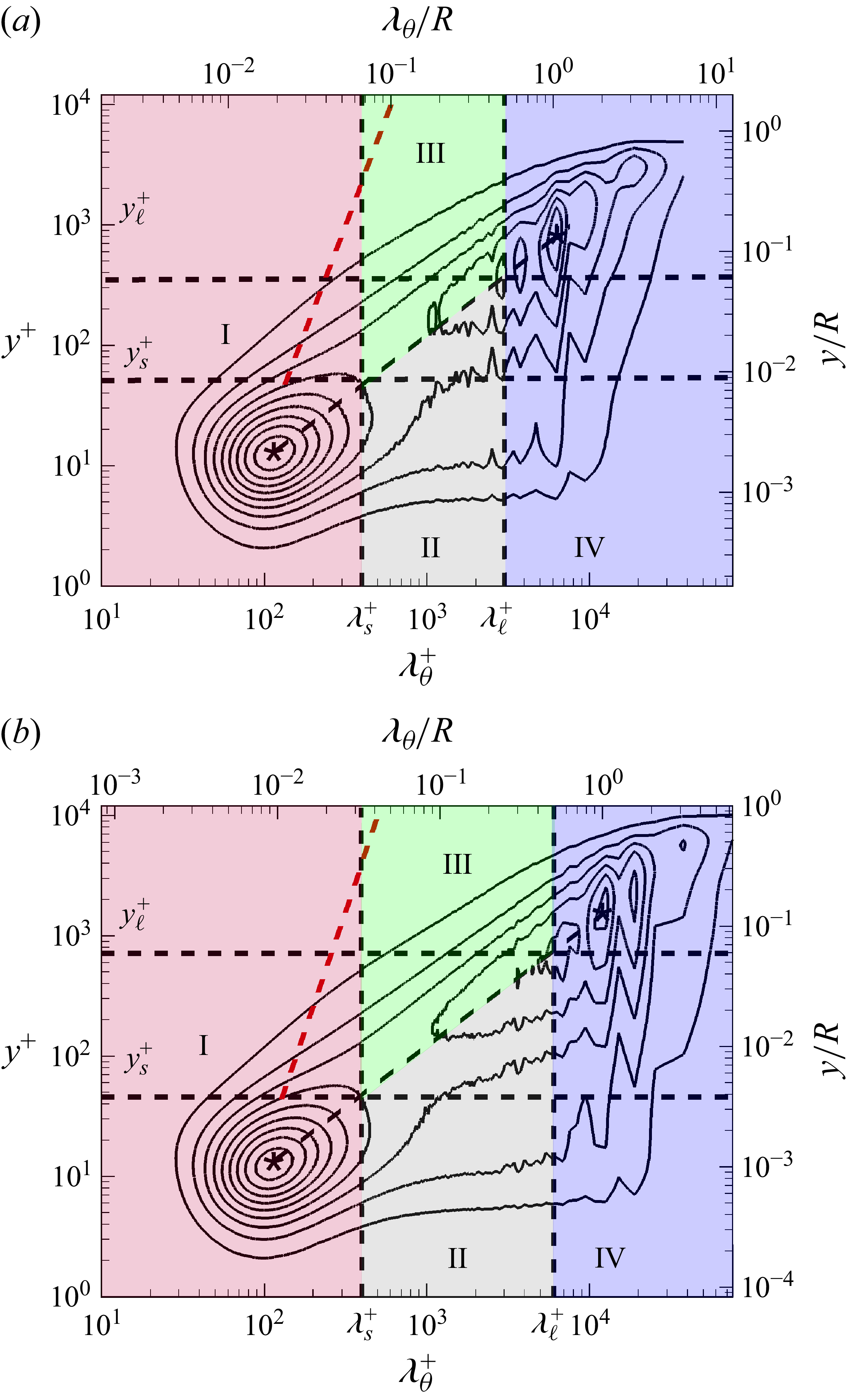
 Reτ≈6000
 Reτ≈12000
 kθ+Euu+
 0.36
0.36 3.6
3.6 0.36
0.36 λS
λS λℓ
λℓ ys
ys yℓ
yℓ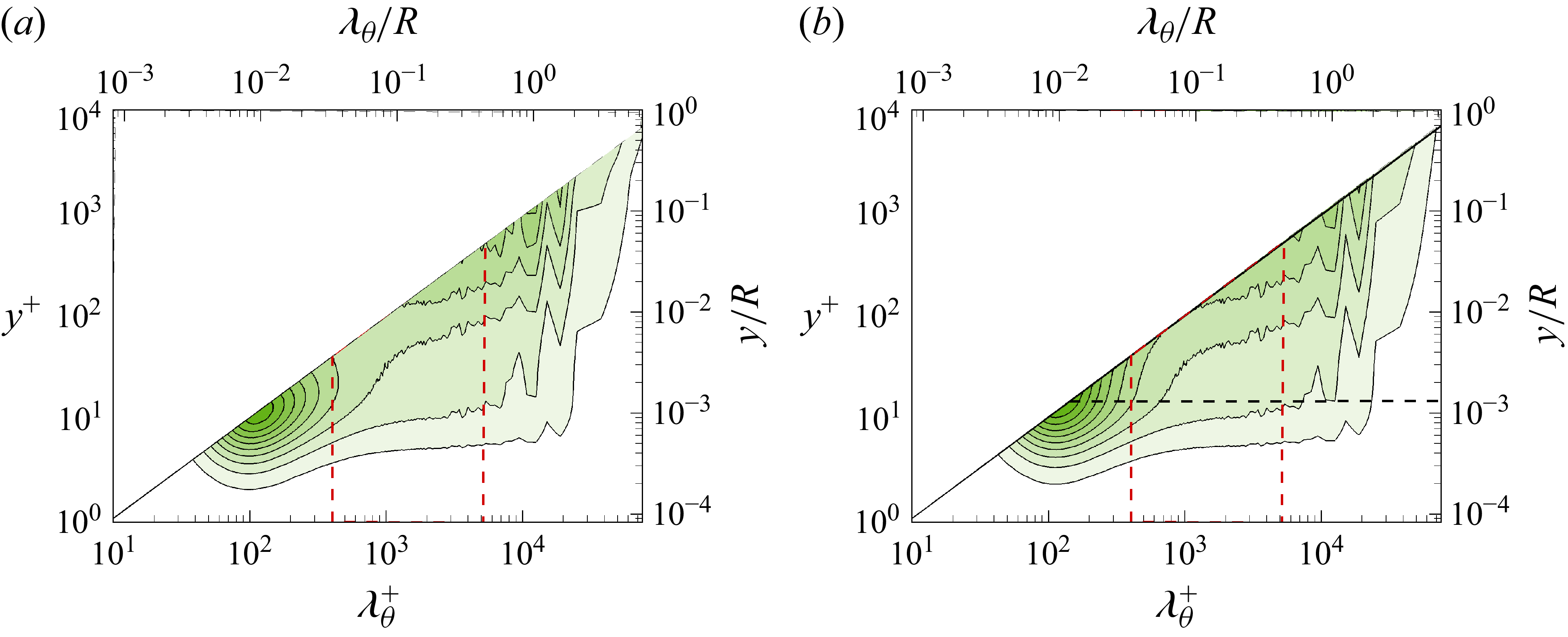
 u
u kθ+Euu+
 0.36
0.36 3.6
3.6 0.36
0.36 y0+=15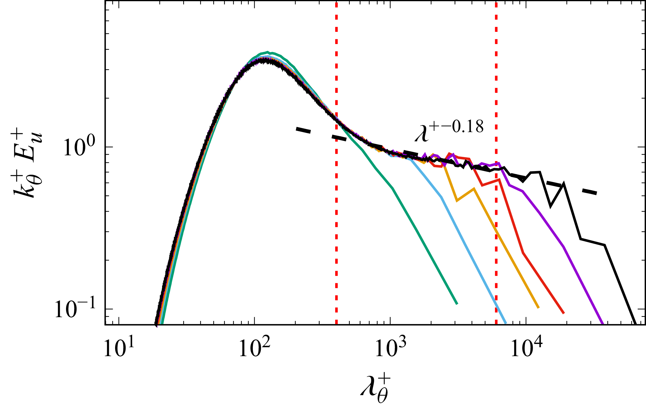
 u
u y0+=15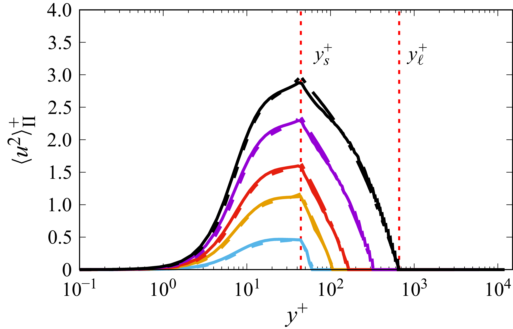
 ys+
ys+ yℓ+
yℓ+
 u
u λ+
λ+ ζ=βλ/y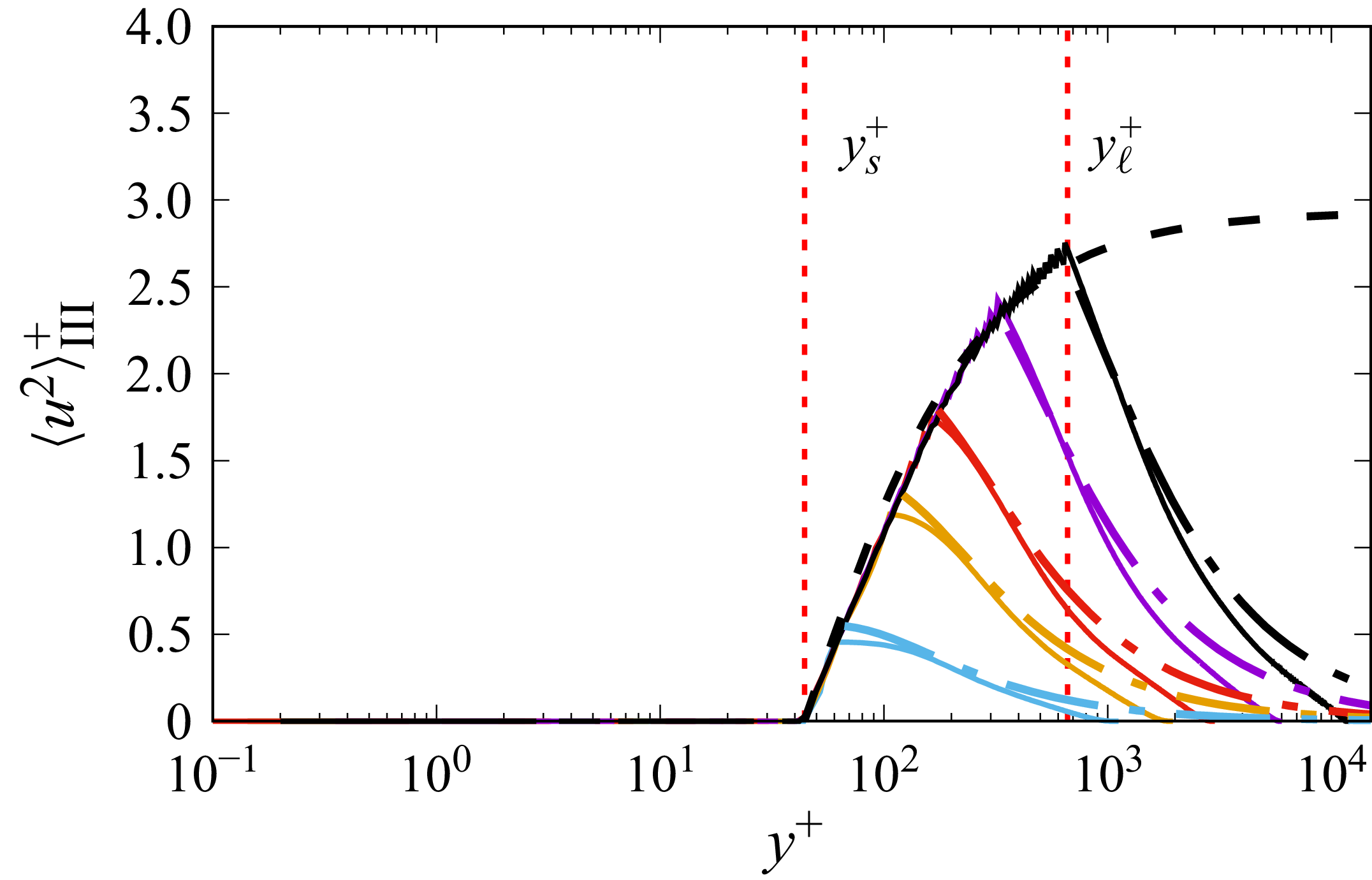
 ys+
ys+ yℓ+
yℓ+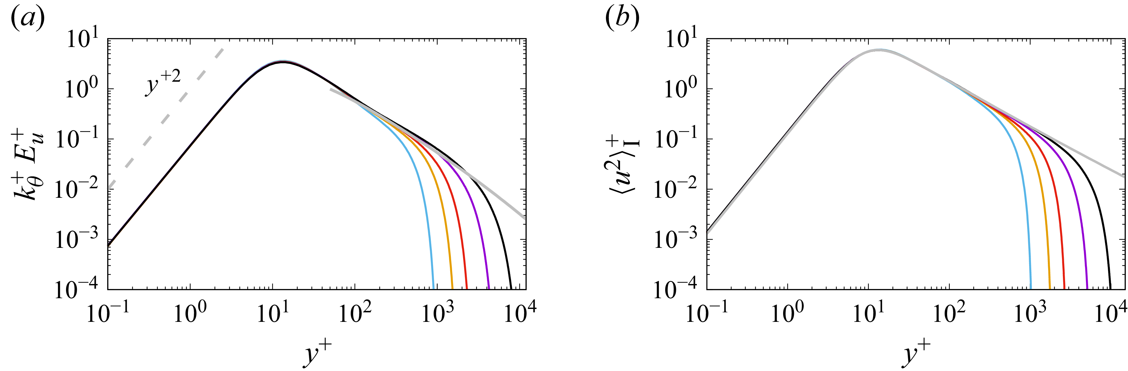
 u
u λ+=136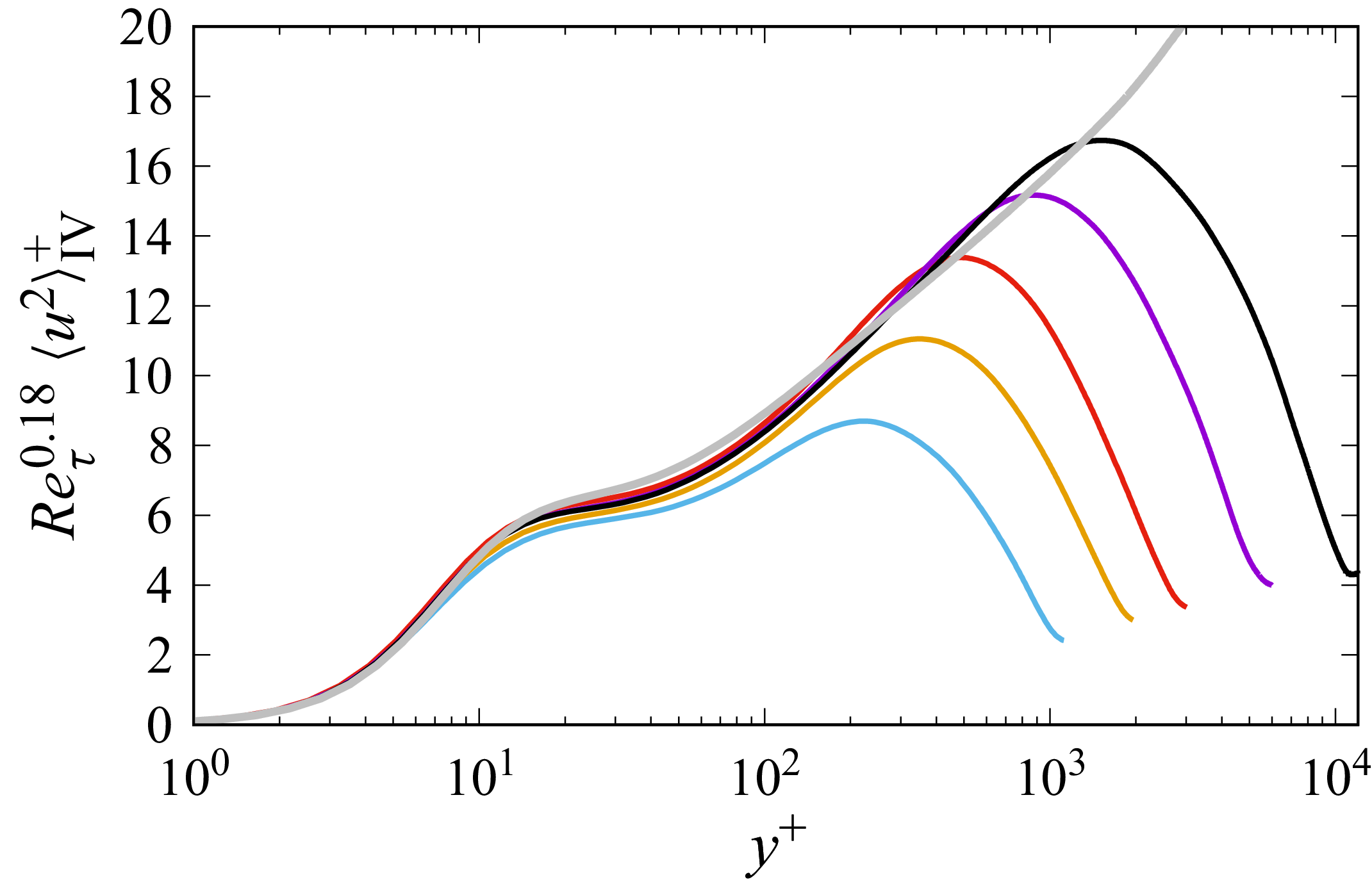
 Reτα
Reτα α=0.18
 D=0.025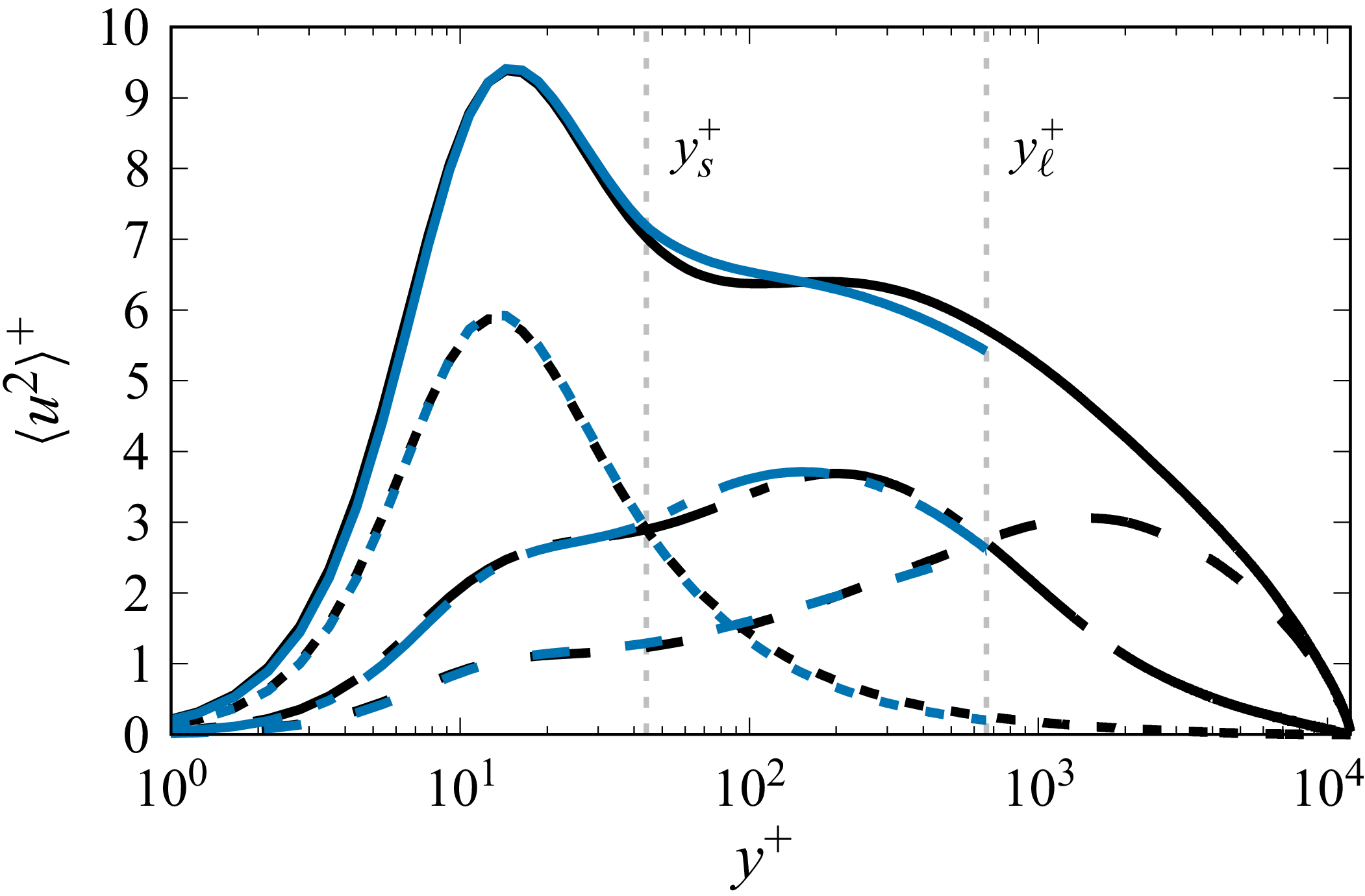
 ys+
ys+ yℓ+
yℓ+
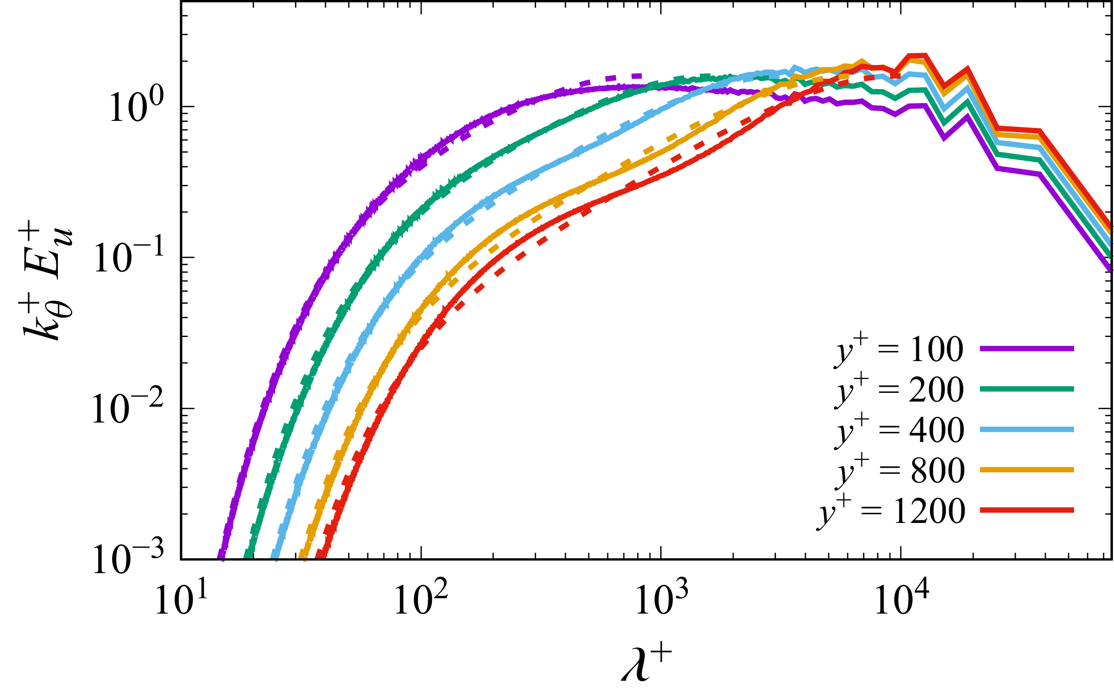
 u
u
 Open access

