


1. Introduction
There are multiple methods to manufacture thin glass sheets (Shelby Reference Shelby2005). The float glass process (Pilkington Reference Pilkington1969; Pop Reference Pop2005; Berenjian & Whittleston Reference Berenjian and Whittleston2017), in which molten glass is fed onto a bath of molten tin and drawn through rollers, gives exceptionally smooth, high quality glass sheets with thickness typically ranging from 2 to 20 mm. Thinner glass sheets can be produced using the down-draw method (Overton Reference Overton2012), in which a ribbon of molten glass is drawn through an annealing furnace before being cooled and removed, resulting in sheet thickness ranging from 20 $\unicode{x03BC} \textrm{m}$
to 1.1
$\unicode{x03BC} \textrm{m}$
to 1.1 $\textrm{mm}$
. Despite the long history of glass sheet manufacture, and the progressive refinement of manufacturing processes, ripples (i.e. sinuous deformations) can still form in the molten glass during production, compromising quality and adding cost. Real-time analysis of the ripple formation is difficult due to the high working temperature of molten glass, and so mathematical modelling is invaluable in the analysis of problems in production.
$\textrm{mm}$
. Despite the long history of glass sheet manufacture, and the progressive refinement of manufacturing processes, ripples (i.e. sinuous deformations) can still form in the molten glass during production, compromising quality and adding cost. Real-time analysis of the ripple formation is difficult due to the high working temperature of molten glass, and so mathematical modelling is invaluable in the analysis of problems in production.
In principle, the origin of the observed ripples is understood. In the industrially relevant limit where the sheet thickness is much smaller than its typical in-plane dimensions, perturbation methods can be used to reduce the governing Navier–Stokes equations and free boundary conditions to a simplified quasi-two-dimensional model that depends on integrated tensions and bending moments (e.g. Howell Reference Howell1996). As shown by Filippov & Zheng (Reference Filippov and Zheng2010), in a down-drawn viscous sheet, regions naturally form in which one of the principal in-plane tensions changes sign, causing a change of type from elliptic to hyperbolic in the underlying partial differential equation governing the sheet centre-surface. The ‘hyperbolic zones’ correspond to regions under compression and are associated with transverse buckling. Srinivasan, Wei & Mahadevan (Reference Srinivasan, Wei and Mahadevan2017) find the fastest growing out-of-plane eigenmodes for the early-time growth of ripples in the sheet. Perdigou & Audoly (Reference Perdigou and Audoly2016) consider a sheet falling under gravity into a bath of fluid and calculate the buckling modes by solving a two-dimensional eigenvalue problem using finite element methods.
The coupled heat transfer and fluid flow for the drawing of a viscous sheet are considered by Scheid et al. (Reference Scheid, Quiligotti, Tran and Stone2009), who find that cooling has a destabilising effect when heat transfer with the air dominates, but has a stabilising effect when both advection and heat transfer with air are important. Thermal effects are also often incorporated simply by treating the viscosity as a function of position, as opposed to solving the coupled energy problem (e.g. Pfingstag, Audoly & Boudaoud Reference Pfingstag, Audoly and Boudaoud2011; Srinivasan et al. Reference Srinivasan, Wei and Mahadevan2017).
In the present paper, we consider the simple model problem of a thin isothermal sheet of viscous fluid retracting freely under surface tension. Despite the absence of any external forcing whatsoever, we show that compressive tensions form generically, and that they can be sufficiently strong to drive growth in sinuous perturbations of the sheet centre-surface. The linear stability analyses performed in previous studies leave open the question of how the amplitude of any transverse ripples is determined in practice. There seem to be two possible mechanisms: either geometrically nonlinear effects cause the growth to saturate (see, e.g., O’Kiely et al. Reference O’Kiely, Breward, Griffiths, Howell and Lange2019), or convection through the compressive regions, where the centre-surface is predicted to be unstable, limits the exponential growth. In this paper, we neglect nonlinearity, but include convection by the underlying flow, and find transient rather than exponential growth in the centre-surface displacement.
The surface-tension-driven retraction of a thin viscous sheet has been well studied. In the inertial limit, fluid collects in a rim at the edge of the sheet. However, when the Reynolds number is sufficiently small, simulations and experiments show that the sheet instead retracts uniformly (Debrégeas et al. Reference Debrégeas, Martin and Brochard-Wyart1995; Brenner & Gueyffier Reference Brenner and Gueyffier1999; Sünderhauf et al. Reference Sünderhauf, Raszillier and Durst2002; Savva Reference Savva2007; Savva & Bush Reference Savva and Bush2009). If the sheet thickness is constant initially, it will therefore remain spatially uniform, and any small initial fluctuations in the thickness are preserved as the sheet retracts. As we will show, it is these thickness fluctuations that can give rise to compressive tensions in the sheet and thus drive transient buckling.
We begin in § 2 by deriving exact integrated conservation equations for a general viscous sheet with no external forcing other than surface tension acting at the free surface. In § 3, we derive effective boundary conditions via a boundary-layer analysis of the region of high curvature at the edge of the sheet, where the in-plane and transverse length-scales are comparable. With this set-up in place, in § 4, we use perturbation methods to derive a simplified model for the retraction of a thin approximately uniform sheet under surface tension. The leading-order equations and boundary conditions are first derived in a general form before being applied to the simple model problem of a disc of viscous fluid, subject to small axisymmetric fluctuations in the thickness. Numerical solutions to these governing equations are presented in § 5, where we find that transient buckling is possible, with selection of the dominant mode determined by a delicate interaction between the imposed initial thickness and centre-surface perturbations. A further asymptotic approximation in § 6, in the limit of large normalised thickness perturbations, allows us to explain this interaction and to predict the thickness and centre-surface perturbations that lead to the greatest transient growth. Finally, in § 7, we discuss our findings and draw our conclusions.
2. Net balance equations
A sketch of a general, viscous sheet, with the in-plane position vector given by $\boldsymbol {\tilde {x}}=(\tilde {x},\tilde {y})$
.
$\boldsymbol {\tilde {x}}=(\tilde {x},\tilde {y})$
.

We start by deriving exact balance equations representing conservation of mass, linear momentum and angular momentum for a thin sheet of incompressible viscous fluid. To this end, we use a tilde to represent in-plane components; for example, let $\boldsymbol {\tilde {x}}$
denote the in-plane position vector so that, with the transverse unit vector being given by
$\boldsymbol {\tilde {x}}$
denote the in-plane position vector so that, with the transverse unit vector being given by $\boldsymbol {k}$
, the position of any point in the sheet may be expressed in the form
$\boldsymbol {k}$
, the position of any point in the sheet may be expressed in the form $\boldsymbol {x}=\boldsymbol {\tilde {x}}+z\boldsymbol {k}$
. We likewise decompose the velocity
$\boldsymbol {x}=\boldsymbol {\tilde {x}}+z\boldsymbol {k}$
. We likewise decompose the velocity $\boldsymbol {u}$
and the stress tensor
$\boldsymbol {u}$
and the stress tensor $\boldsymbol {\sigma }$
into in-plane and transverse components, i.e.
$\boldsymbol {\sigma }$
into in-plane and transverse components, i.e.
 \begin{align} \boldsymbol {u}&=\tilde {\boldsymbol {u}}+w\boldsymbol {k}, & \boldsymbol {\sigma }&=\left ( \begin{array}{c c|c} \tilde {\boldsymbol {\sigma }}& &\hat {\boldsymbol {\sigma }}\\[-5pt] &&\\ \hline&&\\[-5pt] \hat {\boldsymbol {\sigma }}^{t} & & \sigma _{zz} \end{array} \right ). \end{align}
Here, $\tilde {\boldsymbol {\sigma }}\in \mathbb {R}^{2\times 2}$
is the in-plane stress tensor,
$\tilde {\boldsymbol {\sigma }}\in \mathbb {R}^{2\times 2}$
is the in-plane stress tensor, $\hat {\boldsymbol {\sigma }}{\in \mathbb {R}^2}$
is the vector of transverse stresses and
$\hat {\boldsymbol {\sigma }}{\in \mathbb {R}^2}$
is the vector of transverse stresses and $\hat {\boldsymbol {\sigma }}^{t}$
is its transpose. The fluid is assumed to lie between two free surfaces, denoted by
$\hat {\boldsymbol {\sigma }}^{t}$
is its transpose. The fluid is assumed to lie between two free surfaces, denoted by $z=H^\pm (\boldsymbol {\tilde {x}},t):=H(\boldsymbol {\tilde {x}},t)\pm h(\boldsymbol {\tilde {x}},t)/2$
, where
$z=H^\pm (\boldsymbol {\tilde {x}},t):=H(\boldsymbol {\tilde {x}},t)\pm h(\boldsymbol {\tilde {x}},t)/2$
, where $h\gt 0$
and
$h\gt 0$
and $H$
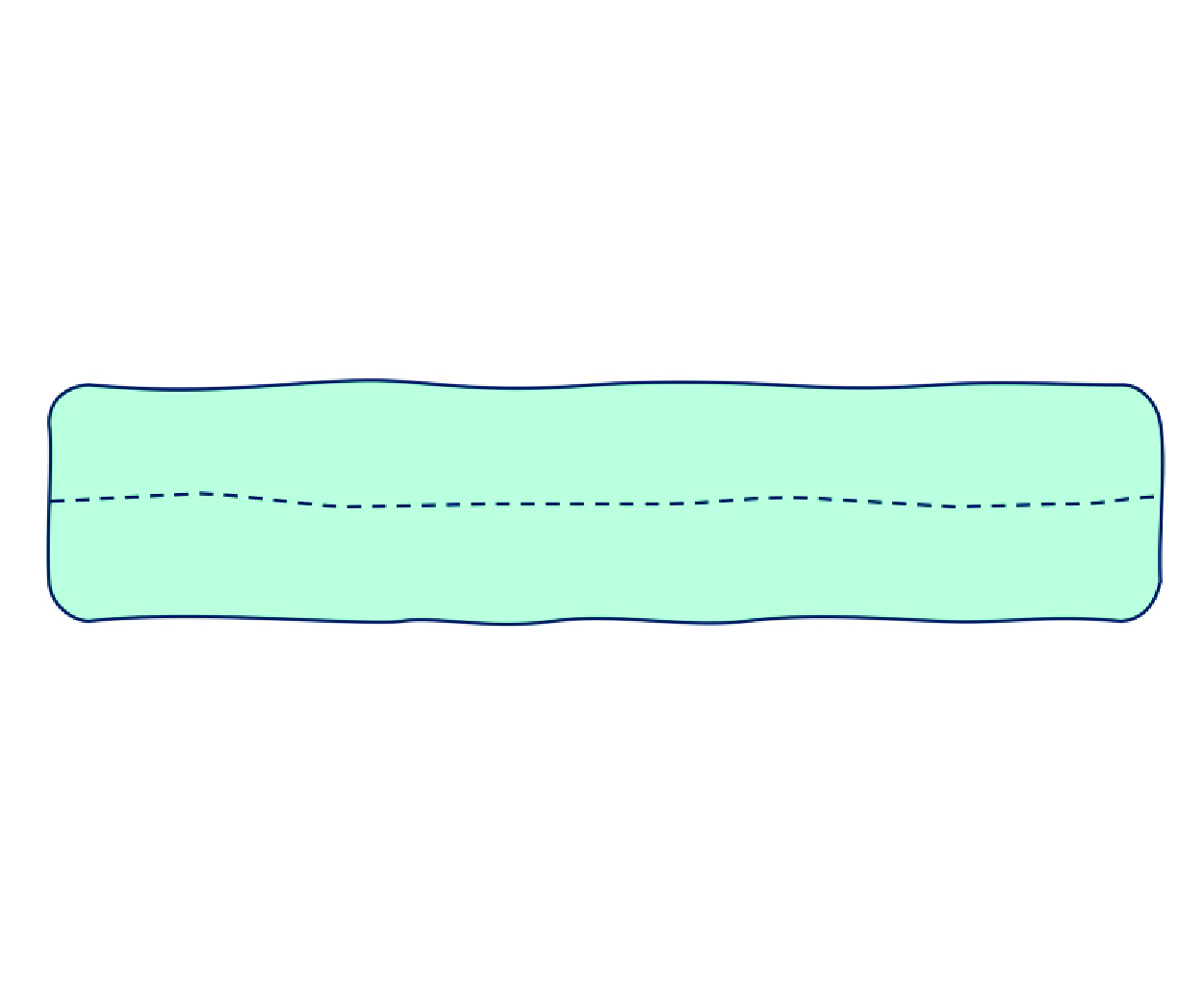
represent the thickness of the sheet and the position of the centre-surface, respectively, as shown in figure 1. To keep this derivation as general as possible, we do not yet make any assumptions about the lateral extent of the sheet. We assume that any external body forces are negligible, so the flow is driven entirely by the constant surface tension
$H$
represent the thickness of the sheet and the position of the centre-surface, respectively, as shown in figure 1. To keep this derivation as general as possible, we do not yet make any assumptions about the lateral extent of the sheet. We assume that any external body forces are negligible, so the flow is driven entirely by the constant surface tension $\gamma$
acting at the free surfaces.
$\gamma$
acting at the free surfaces.
Now, when we express the governing equations and boundary conditions in dimensionless form, the assumed thinness of the sheet is captured by applying differential scalings to in-plane and transverse components of the variables. We denote a typical in-plane lengthscale of the sheet by $L$
and a typical transverse lengthscale by
$L$
and a typical transverse lengthscale by $\epsilon L$
, where
$\epsilon L$
, where $\epsilon \ll 1$
. By balancing surface tension with viscous effects, a suitable scaling for the in-plane velocity is found to be
$\epsilon \ll 1$
. By balancing surface tension with viscous effects, a suitable scaling for the in-plane velocity is found to be $\gamma /\epsilon \eta$
, where
$\gamma /\epsilon \eta$
, where $\eta$
is the constant dynamic viscosity. This velocity scale is the typical speed at which a thin inertia-free sheet would retract under surface tension (Debrégeas et al. Reference Debrégeas, Martin and Brochard-Wyart1995; Griffiths & Howell Reference Griffiths and Howell2007). We use the corresponding convective timescale, and scale the transverse velocity and stress components to obtain balances in the Stokes equations (see below). Thus, we arrive at the scalings
$\eta$
is the constant dynamic viscosity. This velocity scale is the typical speed at which a thin inertia-free sheet would retract under surface tension (Debrégeas et al. Reference Debrégeas, Martin and Brochard-Wyart1995; Griffiths & Howell Reference Griffiths and Howell2007). We use the corresponding convective timescale, and scale the transverse velocity and stress components to obtain balances in the Stokes equations (see below). Thus, we arrive at the scalings
 \begin{align} \boldsymbol {\tilde {x}}&=L{\boldsymbol {\tilde {x}}}', & z&=\epsilon L z', & t&=\frac {\epsilon L\eta }{\gamma }\,t' \end{align}
 \begin{align} \tilde {\boldsymbol {u}}&=\frac {\gamma }{\epsilon \eta }\,{\tilde {\boldsymbol {u}}}', & w&=\frac {\gamma }{\eta }\, w', & \left (H,h,H^\pm \right )&=\epsilon L \left (H',h',{H^\pm }'\right ), \end{align}
 \begin{align} \boldsymbol {\tilde {\sigma }}&=\frac {\gamma }{\epsilon L}\,\boldsymbol {\tilde {\sigma }}', & \boldsymbol {\hat {\sigma }}&=\frac {\gamma }{L}\,\boldsymbol {\hat {\sigma }}', & \sigma _{zz}&=\frac {\epsilon \gamma }{L}\,\sigma _{zz}'. \end{align}
In the dimensionless equations presented below, the prime decoration is dropped.
We assume that inertia and any body forces are negligible, so the flow is governed by the dimensionless incompressible Stokes equations, which take the forms
 \begin{align} \tilde {\boldsymbol {\nabla }}\cdot \tilde {\boldsymbol {u}} +\frac {\partial w}{\partial z}&=0, & \tilde {\boldsymbol {\nabla }}\cdot \tilde {\boldsymbol {\sigma }} +\frac {\partial \hat {\boldsymbol {\sigma }}}{\partial z}&=\boldsymbol {0}, & \tilde {\boldsymbol {\nabla }}\cdot \hat {\boldsymbol {\sigma }} +\frac {\partial \sigma _{zz}}{\partial z}&=0, \end{align}
following our decompositions, where $\tilde {\boldsymbol {\nabla }}$
denotes the in-plane gradient operator. At the two free surfaces
$\tilde {\boldsymbol {\nabla }}$
denotes the in-plane gradient operator. At the two free surfaces $z=H^\pm$
, we apply the kinematic boundary condition
$z=H^\pm$
, we apply the kinematic boundary condition
 \begin{equation} w=\frac {\partial H^\pm }{\partial t}+\tilde {\boldsymbol {u}}\cdot \tilde {\boldsymbol {\nabla }} H^\pm , \end{equation}
and the dynamic boundary condition, which may be decomposed into
 \begin{align} \tilde {\boldsymbol {\sigma }}\cdot \tilde {\boldsymbol {\nabla }} H^\pm + \epsilon ^2 \kappa ^\pm \tilde {\boldsymbol {\nabla }} H^\pm & = \hat {\boldsymbol {\sigma }}, \end{align}
 \begin{align} \sigma _{zz}+\kappa ^\pm &=\hat {\boldsymbol {\sigma }}\cdot \tilde {\boldsymbol {\nabla }} H^\pm . \end{align}
Without loss of generality, the constant external pressure has been set to zero. The free-surface curvatures are given by
 \begin{align} \kappa ^\pm &=\mp \,\tilde {\boldsymbol {\nabla }}\cdot \left (\frac {\tilde {\boldsymbol {\nabla }} H^\pm }{\triangle ^\pm }\right ), \qquad \text {where} \quad \triangle ^\pm =\sqrt {1+\epsilon ^2\left |\tilde {\boldsymbol {\nabla }} H^\pm \right |^2}. \end{align}
Integrating the continuity equation (2.3a ) across the thickness and applying the kinematic boundary condition (2.4), we obtain the net mass conservation equation
 \begin{equation} \frac {\partial h}{\partial t}+\tilde {\boldsymbol {\nabla }}\cdot \left (h\boldsymbol {\bar {u}}\right )=0, \end{equation}
where
 \begin{equation} \boldsymbol {\bar {u}}=\frac {1}{h}\int _{H^-}^{H^+} \tilde {\boldsymbol {u}} \, \mathrm {d}z \end{equation}
is the average in-plane velocity.
Integrating the in-plane component of the momentum equation (2.3b ) and applying the dynamic boundary condition (2.5a ) gives
 \begin{equation} \tilde {\boldsymbol {\nabla }}\cdot \boldsymbol{T}\,=\boldsymbol {0}, \end{equation}
where we define the in-plane tension tensor by
 \begin{equation} \boldsymbol{T}\,= \int _{H^-}^{H^+} \tilde {\boldsymbol {\sigma }} \, \mathrm {d}z +\left [(\triangle ^++\triangle ^-)\boldsymbol{I}\,{-}\,\frac {\epsilon ^2(\tilde {\boldsymbol {\nabla }} H^+)(\tilde {\boldsymbol {\nabla }} H^+)^t}{\triangle ^+}-\frac {\epsilon ^2(\tilde {\boldsymbol {\nabla }} H^-)(\tilde {\boldsymbol {\nabla }} H^-)^t}{\triangle ^-}\right ]. \end{equation}
The first integral term on the right-hand side of (2.10) is the viscous contribution to the tension, while the term in square brackets is the contribution due to surface tension. Similarly, by integrating the out-of-plane component of the momentum equation (2.3c ) and applying the dynamic boundary condition (2.5b ), we obtain
 \begin{equation} \tilde {\boldsymbol {\nabla }}\cdot \boldsymbol{N}\,\,{=}\,0, \end{equation}
where we define the total shear stress by
 \begin{equation} \boldsymbol{N}\,\,{=}\, \int _{H^-}^{H^+} \hat {\boldsymbol {\sigma }} \, \mathrm {d}z + \left [ \frac {\tilde {\boldsymbol {\nabla }} H^+}{\triangle ^+}+\frac {\tilde {\boldsymbol {\nabla }} H^-}{\triangle ^-}\right ]. \end{equation}
Finally, by multiplying the in-plane component of the momentum equation (2.3b
) by $(z-H)$
before integrating over the thickness, we derive the torque balance equation
$(z-H)$
before integrating over the thickness, we derive the torque balance equation
 \begin{equation} \tilde {\boldsymbol {\nabla }}\cdot \boldsymbol{M}\,{+}\,\boldsymbol{T}\,\cdot \tilde {\boldsymbol {\nabla }} H=\boldsymbol{N}, \end{equation}
where the bending-moment tensor is defined by
 \begin{equation} \boldsymbol{M}\,\,{=}\,\int _{H^-}^{H^+} (z-H)\tilde {\boldsymbol {\sigma }} \, \mathrm {d}z +\frac {h}{2}\left [(\triangle ^+-\triangle ^-)\boldsymbol{I}\,{-}\,\frac {\epsilon ^2(\tilde {\boldsymbol {\nabla }} H^+)(\tilde {\boldsymbol {\nabla }} H^+)^t}{\triangle ^+}+\frac {\epsilon ^2(\tilde {\boldsymbol {\nabla }} H^-)(\tilde {\boldsymbol {\nabla }} H^-)^t}{\triangle ^-}\right ]. \end{equation}
The basic governing equations for the evolution of a thin sheet of viscous fluid under surface tension are (2.7), (2.9), (2.11) and (2.13). We emphasise that no approximations have been made yet, so these net balance equations are exact, and that the contributions from surface tension have been incorporated into the definitions of the integrated stress and moment tensors. This approach was found to be beneficial by Griffiths & Howell (Reference Griffiths and Howell2007) when studying the surface-tension-driven evolution of a tube of viscous fluid, and we will show in the next section how it pays off when deriving the effective boundary conditions at a sheet edge.
To close the problem (2.7), (2.9), (2.11) and (2.13), it remains to derive constitutive relations for $\boldsymbol{T}$
and
$\boldsymbol{T}$
and $\boldsymbol{M}$
in terms of
$\boldsymbol{M}$
in terms of $\boldsymbol {\bar {u}}$
,
$\boldsymbol {\bar {u}}$
, $h$
and
$h$
and $H$
, by exploiting the assumed smallness of
$H$
, by exploiting the assumed smallness of $\epsilon$
. In previous studies of viscous buckling (e.g. Buckmaster, Nachman & Ting Reference Buckmaster, Nachman and Ting1975; Howell Reference Howell1996; Ribe Reference Ribe2002), two possible dominant balances have been identified. The sheet thickness
$\epsilon$
. In previous studies of viscous buckling (e.g. Buckmaster, Nachman & Ting Reference Buckmaster, Nachman and Ting1975; Howell Reference Howell1996; Ribe Reference Ribe2002), two possible dominant balances have been identified. The sheet thickness $h$
evolves over an
$h$
evolves over an $O(1)$
‘stretching’ timescale, while transverse sheet motion occurs over an
$O(1)$
‘stretching’ timescale, while transverse sheet motion occurs over an $O (\epsilon ^2 )$
‘bending’ timescale. In contrast with these previous studies, we will show that, when the leading-order sheet thickness is spatially uniform, bending and stretching occur on the same
$O (\epsilon ^2 )$
‘bending’ timescale. In contrast with these previous studies, we will show that, when the leading-order sheet thickness is spatially uniform, bending and stretching occur on the same $O(1)$
timescale.
$O(1)$
timescale.
3. Edge boundary layer
3.1. Motivation and local coordinate system
In § 2, we derived the general net balance equations for a thin sheet of viscous fluid. Now, we show how to supplement these equations with effective boundary conditions that apply at a free edge of the sheet. Near such an edge, there is a boundary layer in which the in-plane and transverse dimensions of the sheet become comparable, as illustrated in figure 2(a). We note that the solution for the flow in this inner region was found numerically by Munro & Lister (Reference Munro and Lister2018), but we show that the effective boundary conditions for the bulk flow can be obtained just using asymptotic matching. In this derivation, we consider the general situation where the edge of the sheet can be arbitrarily curved, though, for simplicity, we assume that it remains approximately planar. We use intrinsic curvilinear coordinates embedded in the sheet edge; a similar derivation is presented by O’Kiely (Reference O’Kiely2017), though without the inclusion of surface tension. Since the problem is quasi-steady, we can focus on determining the instantaneous boundary conditions and, for the moment, suppress the dependence on time $t$
.
$t$
.
(a) Sketch of the inner region at the edge of a thin sheet. (b) Sketch of the curvilinear coordinate system employed at the edge of the sheet.

An edge of the sheet is identified as a curve on which $h=0$
. As illustrated in figure 2(b), we parametrise the projection of this curve onto the
$h=0$
. As illustrated in figure 2(b), we parametrise the projection of this curve onto the $\boldsymbol {\tilde {x}}=(\tilde {x},\tilde {y})$
-plane using arc-length
$\boldsymbol {\tilde {x}}=(\tilde {x},\tilde {y})$
-plane using arc-length $s$
, and denote the corresponding planar tangent vector as
$s$
, and denote the corresponding planar tangent vector as $\boldsymbol {\tilde {t}}(s)$
. We fix the orientation such that the planar normal pointing outwards from the sheet edge is given by
$\boldsymbol {\tilde {t}}(s)$
. We fix the orientation such that the planar normal pointing outwards from the sheet edge is given by $\boldsymbol {\tilde {n}}=\boldsymbol {k}\times \boldsymbol {\tilde {t}}$
, where we recall that
$\boldsymbol {\tilde {n}}=\boldsymbol {k}\times \boldsymbol {\tilde {t}}$
, where we recall that $\boldsymbol {k}$
denotes the unit vector in the
$\boldsymbol {k}$
denotes the unit vector in the $z$
-direction. The normal and tangent vectors are related by the Serret–Frenet formulae (Kreyszig Reference Kreyszig1959)
$z$
-direction. The normal and tangent vectors are related by the Serret–Frenet formulae (Kreyszig Reference Kreyszig1959)
 \begin{align} \frac {\mathrm {d}\boldsymbol {\tilde {t}}}{\mathrm {d}s}&=\kappa \boldsymbol {\tilde {n}}, & \frac {\mathrm {d}\boldsymbol {\tilde {n}}}{\mathrm {d}s}&=-\kappa \boldsymbol {\tilde {t}}, \end{align}
where $\kappa (s)$
is the curvature of the edge (projected onto the
$\kappa (s)$
is the curvature of the edge (projected onto the $(\tilde{x},\tilde{y})$
-plane). The position of any point in the sheet can be expressed in the form
$(\tilde{x},\tilde{y})$
-plane). The position of any point in the sheet can be expressed in the form
 \begin{equation} \boldsymbol {r}(s,n,z)=\boldsymbol {\tilde {x}}+z\boldsymbol {k}=\int _0^s \boldsymbol {\tilde {t}}(s^\prime )\, \mathrm {d}s^\prime + n\boldsymbol {\tilde {n}}+z\boldsymbol {k}, \end{equation}
where $n\lt 0$
and
$n\lt 0$
and $H^-(s,n)\lt z\lt H^+(s,n)$
. The edge of the sheet is defined to be at
$H^-(s,n)\lt z\lt H^+(s,n)$
. The edge of the sheet is defined to be at $n=0$
, where we have
$n=0$
, where we have $H^-(s,0)=H^+(s,0)=H(s,0)$
.
$H^-(s,0)=H^+(s,0)=H(s,0)$
.
Now, our strategy is to express the integrated governing equations (2.9), (2.11) and (2.13) using the local coordinates $(s,n)$
. Then, at the edge of the sheet, since
$(s,n)$
. Then, at the edge of the sheet, since $h(s,0)=0$
, we seemingly have five boundary conditions
$h(s,0)=0$
, we seemingly have five boundary conditions
 \begin{equation} T_{nn}=T_{sn}={N_n}=M_{nn}=M_{sn}=0 \quad \text {at }n=0{,} \end{equation}
where subscripts denote components of the tensor or vector. However, this is one too many boundary conditions for the outer problem. This issue was first addressed in the context of thin elastic plates (see, for example, Love Reference Love1927; Timoshenko & Woinowsky-Krieger Reference Timoshenko and Woinowsky-Krieger1959). We resolve the difficulty by rescaling into the boundary layer at the edge and thus deriving the appropriate effective boundary conditions to apply to the outer problem.
3.2. Edge boundary layer
We examine the boundary layer by defining
 \begin{align} \kern-4em n=\epsilon \hat {n}, \qquad T_{ss}=\hat {T}_{ss}, \qquad T_{sn}=\epsilon \hat {T}_{sn}, \qquad T_{nn}=\epsilon \hat {T}_{nn}, \end{align}
 \begin{align} M_{ss}=\hat {M}_{ss}, \qquad M_{sn}=\hat {M}_{sn}, \qquad M_{nn}=\epsilon \hat {M}_{nn}, \qquad N_s = \frac {\hat {N}_s}{\epsilon }, \qquad N_n = \hat {N}_n, \end{align}
where we denote variables in the boundary layer by hats (not to be confused with the transverse stress components as in § 2). The different scalings of the tensions, shears and bending moments are made to obtain non-trivial balances in the dimensionless integrated Stokes equations, (2.9), (2.11) and (2.13), which become (see, for example, van de Fliert, Howell & Ockendon Reference van de Fliert, Howell and Ockendon1995)
 \begin{align} \frac {\partial \hat {T}_{ss}}{\partial s}+\frac {\partial }{\partial \hat {n}}(\hat {\ell } \hat {T}_{sn})-\epsilon \kappa \hat {T}_{sn}&= 0, \end{align}
 \begin{align} \epsilon \frac {\partial \hat {T}_{sn}}{\partial s}+\frac {\partial }{\partial \hat {n}}(\hat {\ell } \hat {T}_{nn})+\kappa \hat {T}_{ss}&= 0, \end{align}
 \begin{align} {\frac {\partial \hat {N}_{s}}{\partial s}+\frac {\partial }{\partial \hat {n}}(\hat {\ell } \hat {N}_{n})} &= 0, \end{align}
 \begin{align} \kern 20pt\epsilon \frac {\partial }{\partial s}\left (\hat {M}_{ss}+\hat {H} \hat {T}_{ss}\right )+\frac {\partial }{\partial \hat {n}}\left [\hat {\ell }\left (\hat {M}_{sn}+\epsilon \hat {H}\hat {T}_{sn}\right )\right ]-\epsilon \kappa \left (\hat {M}_{sn}+\epsilon\!\hat {H}\hat {T}_{sn}\right ) & = \hat {\ell } {\hat {N}_{s}}, \end{align}
 \begin{align} \frac {\partial }{\partial s}\left (\hat {M}_{sn}+\epsilon \hat {H} \hat {T}_{sn}\right )+\frac {\partial }{\partial \hat {n}}\left [\hat {\ell }\left (\hat {M}_{nn}+\hat {H}\hat {T}_{nn}\right )\right ]+\kappa \left (\hat {M}_{ss}+\hat {H}\hat {T}_{ss}\right ) & = \hat {\ell } {\hat {N}_{n}}, \end{align}
where $\hat {\ell }=1-\epsilon \kappa \hat {n}$
is the metric coefficient. The boundary conditions (3.3) at the edge of the sheet are transformed to
$\hat {\ell }=1-\epsilon \kappa \hat {n}$
is the metric coefficient. The boundary conditions (3.3) at the edge of the sheet are transformed to
 \begin{equation} \hat {T}_{nn}=\hat {T}_{sn}={\hat {N}_{n}}=\hat {M}_{nn}=\hat {M}_{sn}=0 \quad \text {at }\hat {n}=0. \end{equation}
We now expand our variables as asymptotic series in powers of $\epsilon$
, i.e.
$\epsilon$
, i.e. $\hat {T}_{ss}\sim \hat {T}_{ss0}+\epsilon \hat {T}_{ss1}+\cdots$
as
$\hat {T}_{ss}\sim \hat {T}_{ss0}+\epsilon \hat {T}_{ss1}+\cdots$
as $\epsilon \to 0$
. Note that the scalings (3.4) already assume the leading-order matching conditions
$\epsilon \to 0$
. Note that the scalings (3.4) already assume the leading-order matching conditions
 \begin{align} T_{sn0},\, T_{nn0},\, M_{nn0}\to 0 \quad \textrm {as } n\to 0,&&&{\hat {N}_{s0}}\to 0 \quad \textrm {as }\hat {n}\to -\infty . \end{align}
As anticipated above and suggested by the sketch in figure 2(a), we also assume that, although the sheet thickness $h$
varies significantly in the edge layer, the centre-surface
$h$
varies significantly in the edge layer, the centre-surface $H$
does not, so that
$H$
does not, so that $\hat {H}(s,n)\sim \hat {H}_0(s)+O(\epsilon )$
.
$\hat {H}(s,n)\sim \hat {H}_0(s)+O(\epsilon )$
.
At leading order, we find from (3.5d ) that
 \begin{equation} {\hat {N}_{s0}}=\frac {\partial \hat {M}_{sn0}}{\partial \hat {n}}. \end{equation}
Substituting this result into (3.5c ) gives, at leading order,
 \begin{equation} \frac {\partial }{\partial \hat {n}}\left ({\hat {N}_{n0}}+\frac {\partial \hat {M}_{sn0}}{\partial s}\right )=0. \end{equation}
By applying the boundary conditions (3.6), we deduce that
 \begin{equation} {\hat {N}_{n0}}+\frac {\partial \hat {M}_{sn0}}{\partial s}=0, \end{equation}
and, by matching to the outer region, we deduce the leading-order effective boundary condition
 \begin{equation} {\hat {N}_{n0}}+\frac {\partial M_{sn0}}{\partial s}=0\quad \textrm {at }n=0. \end{equation}
However, by combining (3.5b ) and (3.5e ) at leading order, we obtain
 \begin{equation} {\hat {N}_{n0}}=\frac {\partial \hat {M}_{sn0}}{\partial s} +\frac {\partial \hat {M}_{nn0}}{\partial \hat {n}} +\kappa \hat {M}_{ss0}, \end{equation}
which can be used to eliminate the shear stress and express (3.11) purely in terms of the bending-moment tensor. In summary, we can express the leading-order effective boundary conditions for the outer problem as
 \begin{equation} T_{sn}=T_{nn}=M_{nn}=2\frac {\partial M_{sn}}{\partial s}+\frac {\partial M_{nn}}{\partial n}+\kappa M_{ss}=0\qquad \textrm {at }n=0. \end{equation}
A benefit of this method, when compared with similar derivations carried out by Howell, Kozyreff & Ockendon (Reference Howell, Kozyreff and Ockendon2009)and O’Kiely (Reference O’Kiely2017), for example, is that we did not need to calculate any velocity components of the fluid; instead, we worked with the tensions and bending moments. Moreover, incorporating surface tension contributions into the definitions of the net tensions and bending moments made it straightforward to generalise the boundary conditions found by O’Kiely (Reference O’Kiely2017) to include surface tension effects. We note that an alternative derivation of the effective boundary conditions based on a virtual work argument is presented by Srinivasan et al. (Reference Srinivasan, Wei and Mahadevan2017), though there appear to be some sign inconsistencies in their formulation.
Armed with the boundary conditions (3.13), we are ready to tackle the outer governing equations (2.7), (2.9), (2.11) and (2.13). As noted in § 2, we must first derive constitutive relations for the integrated tensions and bending moments by analysing the asymptotic limit as $\epsilon \rightarrow 0$
. In doing so, we choose to focus on a model geometrical set-up in which a disc of viscous fluid retracts under surface tension, and then examine the response of the system to small transverse perturbations.
$\epsilon \rightarrow 0$
. In doing so, we choose to focus on a model geometrical set-up in which a disc of viscous fluid retracts under surface tension, and then examine the response of the system to small transverse perturbations.
4. Model for an approximately uniform viscous sheet
4.1. Leading-order solution
Now, we invoke the dimensionless Newtonian constitutive relations, namely
 \begin{align} \tilde {\boldsymbol {\sigma }}&=-p\tilde {\boldsymbol {I}}+\tilde {\boldsymbol {\nabla }}\tilde {\boldsymbol {u}}+{\tilde {\boldsymbol {\nabla }}\tilde {\boldsymbol {u}}}^t, & \epsilon ^2\sigma _{zz}&=-p-2\tilde {\boldsymbol {\nabla }}\cdot \tilde {\boldsymbol {u}}, & \epsilon ^2\hat {\boldsymbol {\sigma }}&= \frac {\partial \tilde {\boldsymbol {u}}}{\partial z}+ \epsilon ^2\tilde {\boldsymbol {\nabla }}w, \end{align}
where the pressure $p$
has been made dimensionless with
$p$
has been made dimensionless with $\gamma /\epsilon L$
, the same scaling as the in-plane stress. Here, we have assumed that the viscosity
$\gamma /\epsilon L$
, the same scaling as the in-plane stress. Here, we have assumed that the viscosity $\eta$
is constant; the theory developed below is generalised to include small viscosity variations in Appendix A. When we express the dependent variables as asymptotic expansions of the form
$\eta$
is constant; the theory developed below is generalised to include small viscosity variations in Appendix A. When we express the dependent variables as asymptotic expansions of the form $\tilde {\boldsymbol {u}}\sim \tilde {\boldsymbol {u}}_0+\epsilon ^2\tilde {\boldsymbol {u}}_1+\cdots$
, we immediately see from (4.1c
) that the flow is extensional to leading order, with the in-plane velocity
$\tilde {\boldsymbol {u}}\sim \tilde {\boldsymbol {u}}_0+\epsilon ^2\tilde {\boldsymbol {u}}_1+\cdots$
, we immediately see from (4.1c
) that the flow is extensional to leading order, with the in-plane velocity $\tilde {\boldsymbol {u}}_0$
independent of
$\tilde {\boldsymbol {u}}_0$
independent of $z$
, i.e.
$z$
, i.e.
 \begin{equation} \tilde {\boldsymbol {u}}_0 = \tilde {\boldsymbol {u}}_0\left (\tilde {\boldsymbol {x}},t\right ). \end{equation}
The net mass-conservation equation (2.7) thus reduces to
 \begin{equation} \frac {\partial h_0}{\partial t}+ \tilde {\boldsymbol {\nabla }}\cdot \left (h_0\tilde {\boldsymbol {u}}_0\right )=0. \end{equation}
Next, we use the constitutive relation (4.1a
) to evaluate the leading-order in-plane stress $\tilde {\boldsymbol {\sigma }}_0$
and thus from (2.10), the in-plane tension tensor, namely
$\tilde {\boldsymbol {\sigma }}_0$
and thus from (2.10), the in-plane tension tensor, namely
 \begin{equation} \boldsymbol{T}_0\,{=}\,\left (2+2h_0\tilde {\boldsymbol {\nabla }}\cdot \tilde {\boldsymbol {u}}_0\right )\tilde {\boldsymbol {I}}+h_0\left (\tilde {\boldsymbol {\nabla }}\tilde {\boldsymbol {u}}_0+\tilde {\boldsymbol {\nabla }}\tilde {\boldsymbol {u}}_0^t\right ). \end{equation}
In this expression, the first factor of $2$
is the contribution due to surface tension, and the remaining terms (proportional to
$2$
is the contribution due to surface tension, and the remaining terms (proportional to $h_0$
) are the viscous contributions. Let us denote the region of the
$h_0$
) are the viscous contributions. Let us denote the region of the $\tilde {\boldsymbol {x}}$
-plane occupied by the sheet by
$\tilde {\boldsymbol {x}}$
-plane occupied by the sheet by $\Omega$
, with boundary
$\Omega$
, with boundary $\partial \Omega$
. Then, the governing equation and boundary condition for
$\partial \Omega$
. Then, the governing equation and boundary condition for $\boldsymbol{T}_0$
, namely
$\boldsymbol{T}_0$
, namely
 \begin{align} \tilde {\boldsymbol {\nabla }}\cdot \boldsymbol{T}_0&=\boldsymbol {0} \quad \text {in }\Omega, & \boldsymbol{T}_0\cdot \tilde {\boldsymbol {n}}&=\boldsymbol {0} \quad \text {on }\partial \Omega , \end{align}
follow from (2.9) and (3.13), respectively. In principle, given $h_0$
, the boundary-value problem (4.4) and (4.5) determines both
$h_0$
, the boundary-value problem (4.4) and (4.5) determines both $\boldsymbol{T}_0$
and
$\boldsymbol{T}_0$
and $\tilde {\boldsymbol {u}}_0$
(up to an irrelevant rigid-body motion), and then
$\tilde {\boldsymbol {u}}_0$
(up to an irrelevant rigid-body motion), and then $h_0$
can be stepped forward in time using (4.3).
$h_0$
can be stepped forward in time using (4.3).
In this paper, we focus on the behaviour of a sheet whose thickness is spatially uniform to leading order, i.e. for which
 \begin{equation} h_0\left (\tilde {\boldsymbol {x}},t\right )=\psi (t). \end{equation}
In this case, the problem (4.4) and (4.5) implies that
 \begin{equation} \boldsymbol{T}_0\left (\tilde {\boldsymbol {x}},t\right )=\boldsymbol {0}. \end{equation}
Although the flow is extensional at leading order, the viscous and surface tension terms in (2.10) exactly balance, so the leading-order tension in the sheet is identically zero. Up to an arbitrary rigid-body translation and rotation, the corresponding leading-order velocity is found from (4.4) to be given by
 \begin{equation} \tilde {\boldsymbol {u}}_0\left (\tilde {\boldsymbol {x}},t\right )=-\frac {\tilde {\boldsymbol {x}}}{3\psi (t)}. \end{equation}
Then, the mass-conservation equation (4.3) reduces to $\dot {\psi }-2/3=0$
(with the dot denoting differentiation) and, therefore,
$\dot {\psi }-2/3=0$
(with the dot denoting differentiation) and, therefore,
 \begin{equation} h_0(\tilde {\boldsymbol {x}},t)=\psi (t)=1+\frac {2t}{3}. \end{equation}
In this leading-order solution, the initially uniform sheet thickness remains uniform and grows linearly with $t$
, as the sheet retracts under surface tension. If we define in-plane Lagrangian variables
$t$
, as the sheet retracts under surface tension. If we define in-plane Lagrangian variables $\tilde {\boldsymbol {X}}$
by
$\tilde {\boldsymbol {X}}$
by
 \begin{equation} \tilde {\boldsymbol {x}}=\frac {\tilde {\boldsymbol {X}}}{\sqrt {\psi (t)}}, \end{equation}
then, with respect to $\tilde {\boldsymbol {X}}$
, the sheet domain, which we will now denote by
$\tilde {\boldsymbol {X}}$
, the sheet domain, which we will now denote by $\Omega _X$
, remains fixed for all time. Of course, this result is subject to the caveat that the aspect ratio of the sheet must remain small, which requires that
$\Omega _X$
, remains fixed for all time. Of course, this result is subject to the caveat that the aspect ratio of the sheet must remain small, which requires that $\psi (t)\ll \epsilon ^{-2/3}$
.
$\psi (t)\ll \epsilon ^{-2/3}$
.
4.2. Small thickness perturbations
We have seen that the leading-order tension in the sheet is identically zero when the sheet thickness is spatially uniform. We now introduce small thickness perturbations of order $\epsilon ^2$
which, as we will demonstrate, are sufficient to induce regions of compression and thus the possibility of buckling. To simplify the analysis, we make the change of variables from
$\epsilon ^2$
which, as we will demonstrate, are sufficient to induce regions of compression and thus the possibility of buckling. To simplify the analysis, we make the change of variables from $ (\tilde {\boldsymbol {x}},z,t )$
to
$ (\tilde {\boldsymbol {x}},z,t )$
to $ (\tilde {\boldsymbol {X}},z,t )$
, where
$ (\tilde {\boldsymbol {X}},z,t )$
, where $\tilde {\boldsymbol {X}}$
are the Lagrangian in-plane variables introduced in (4.10). We then perturb about the above leading-order solution as follows:
$\tilde {\boldsymbol {X}}$
are the Lagrangian in-plane variables introduced in (4.10). We then perturb about the above leading-order solution as follows:
 \begin{align} h\left (\tilde {\boldsymbol {X}},t\right )&\sim \psi (t) +\epsilon ^2h_1\left (\tilde {\boldsymbol {X}},t\right ) +O\bigl (\epsilon ^4\bigr ), \end{align}
 \begin{align} \bar {\boldsymbol {u}}\left (\tilde {\boldsymbol {X}},t\right )&\sim -\frac {\tilde {\boldsymbol {X}}}{3\psi (t)^{3/2}} +\epsilon ^2\bar {\boldsymbol {u}}_1\left (\tilde {\boldsymbol {X}},t\right ) +O\bigl (\epsilon ^4\bigr ), \end{align}
where the initial thickness perturbation $h_1 (\tilde {\boldsymbol {X}},0 )$
is assumed to be specified. We impose the constraint
$h_1 (\tilde {\boldsymbol {X}},0 )$
is assumed to be specified. We impose the constraint
 \begin{equation} \iint _{{\Omega _X}} h_1\left (\tilde {\boldsymbol {X}},0\right )\,\mathrm {d}\tilde {\boldsymbol {X}}=0, \end{equation}
so that the mass of the sheet is accounted for entirely by the leading-order solution.
We also make small perturbations to the centre-surface $H$
, so that
$H$
, so that
 \begin{equation} H\left (\tilde {\boldsymbol {X}},t\right )\sim \delta H_1\left (\tilde {\boldsymbol {X}},t\right ), \end{equation}
where $0\lt \delta \ll 1$
. The initial centre-surface displacement
$0\lt \delta \ll 1$
. The initial centre-surface displacement $\delta H_1 (\tilde {\boldsymbol {X}},0 )$
is again assumed to be specified and small. The restriction to small centre-surface perturbations allows us to linearise about the base state
$\delta H_1 (\tilde {\boldsymbol {X}},0 )$
is again assumed to be specified and small. The restriction to small centre-surface perturbations allows us to linearise about the base state $H=0$
, and the size of
$H=0$
, and the size of $\delta$
in relation to
$\delta$
in relation to $\epsilon$
is irrelevant. The resulting theory models the onset of buckling, should it occur, and remains valid so long as
$\epsilon$
is irrelevant. The resulting theory models the onset of buckling, should it occur, and remains valid so long as $H_1$
remains smaller than
$H_1$
remains smaller than $O (\delta ^{-1} )$
.
$O (\delta ^{-1} )$
.
We recall that the in-plane tension tensor $\boldsymbol{T}$
is zero at leading order, and its asymptotic expansion thus takes the form
$\boldsymbol{T}$
is zero at leading order, and its asymptotic expansion thus takes the form
 \begin{equation} \boldsymbol{T}\left (\tilde {\boldsymbol {X}},t\right )\sim \epsilon ^2\boldsymbol{T}_1\left (\tilde {\boldsymbol {X}},t\right )+O\left (\epsilon ^4,\epsilon ^2\delta ^2\right ). \end{equation}
The first-order in-plane stress $\tilde {\boldsymbol {\sigma }}_1$
is found by substituting the expansions (4.11)–(4.13) into the governing equations (2.3)–(2.5) and constitutive relations (4.1). The first non-zero contribution
$\tilde {\boldsymbol {\sigma }}_1$
is found by substituting the expansions (4.11)–(4.13) into the governing equations (2.3)–(2.5) and constitutive relations (4.1). The first non-zero contribution $\boldsymbol{T}_1$
to the tension is then found from (2.10), which produces
$\boldsymbol{T}_1$
to the tension is then found from (2.10), which produces
 \begin{equation} \boldsymbol{T}_1=2\left (\psi ^{3/2}\tilde {\boldsymbol {\nabla }}\cdot \bar {\boldsymbol {u}}_1-\frac {h_1}{\psi }\right )\tilde {\boldsymbol {I}}+ \psi ^{3/2}\left (\tilde {\boldsymbol {\nabla }}\bar {\boldsymbol {u}}_1+\tilde {\boldsymbol {\nabla }}\bar {\boldsymbol {u}}_1^t\right ), \end{equation}
where, now, the gradient operator $\tilde {\boldsymbol {\nabla }}$
is performed with respect to the new in-plane variables
$\tilde {\boldsymbol {\nabla }}$
is performed with respect to the new in-plane variables $\tilde {\boldsymbol {X}}$
.
$\tilde {\boldsymbol {X}}$
.
The first-order tension satisfies a boundary-value problem analogous to (4.5), that is,
 \begin{align} \tilde {\boldsymbol {\nabla }}\cdot \boldsymbol{T}_1&=\boldsymbol {0} \quad \text {in }{\Omega _X}, & \boldsymbol{T}_1\cdot \tilde {\boldsymbol {n}}&=\boldsymbol {0} \quad \text {on }\partial {\Omega _X} \end{align}
(with no contributions due to perturbations in $\partial {\Omega _X}$
because
$\partial {\Omega _X}$
because $\boldsymbol{T}_0$
is identically zero). As in § 4.1, if
$\boldsymbol{T}_0$
is identically zero). As in § 4.1, if $h_1$
is known, then the problem (4.16) and constitutive relation (4.15) in principle determine both
$h_1$
is known, then the problem (4.16) and constitutive relation (4.15) in principle determine both $\boldsymbol{T}_1$
and
$\boldsymbol{T}_1$
and $\bar {\boldsymbol {u}}_1$
, up to an arbitrary rigid-body motion. The evolution of
$\bar {\boldsymbol {u}}_1$
, up to an arbitrary rigid-body motion. The evolution of $h_1$
is then determined from the first-order mass conservation equation (2.7), namely
$h_1$
is then determined from the first-order mass conservation equation (2.7), namely
 \begin{equation} \frac {\partial h_1}{\partial t}-\frac {2h_1}{3\psi }+\psi ^{3/2}\tilde {\boldsymbol {\nabla }}\cdot \bar {\boldsymbol {u}}_1=0. \end{equation}
We can simplify the problem (4.15)–(4.17) by introducing a scaled Airy stress function $\mathcal {A} (\tilde {\boldsymbol {X}},t )$
such that
$\mathcal {A} (\tilde {\boldsymbol {X}},t )$
such that
 \begin{equation} \boldsymbol{T}_1=\psi ^{-3/4} \mathfrak {H}^{\text {c}}[\mathcal {A}] =\psi ^{-3/4}{\begin{pmatrix} \frac {\partial ^2\mathcal {A}}{\partial Y^2} & -\frac {\partial ^2\mathcal {A}}{\partial X\partial Y} \\[4pt] -\frac {\partial ^2\mathcal {A}}{\partial X\partial Y} & \frac {\partial ^2\mathcal {A}}{\partial X^2} \end{pmatrix}}, \end{equation}
which satisfies (4.16a
) identically. Here, we have introduced the notation $\mathfrak {H}[\cdot ]$
for the two-dimensional Hessian matrix and
$\mathfrak {H}[\cdot ]$
for the two-dimensional Hessian matrix and $\mathfrak {H}^{\text {c}}$
for the corresponding cofactor matrix. By eliminating
$\mathfrak {H}^{\text {c}}$
for the corresponding cofactor matrix. By eliminating $\bar {\boldsymbol {u}}_1$
from (4.15), we find that
$\bar {\boldsymbol {u}}_1$
from (4.15), we find that $\mathcal {A}$
satisfies the forced biharmonic equation
$\mathcal {A}$
satisfies the forced biharmonic equation
 \begin{equation} \tilde {\nabla }^4\mathcal {A}+\psi ^{-1/4}\tilde {\nabla }^2h_1=0, \end{equation}
and the mass-conservation equation (4.17) can be expressed as
 \begin{equation} 6\frac {\partial h_1}{\partial t}+\psi ^{-3/4}\tilde {\nabla }^2\mathcal {A}=0. \end{equation}
By eliminating $\mathcal {A}$
from (4.19) and (4.20), we find that
$\mathcal {A}$
from (4.19) and (4.20), we find that $h_1$
satisfies
$h_1$
satisfies
 \begin{equation} \frac {\partial \tilde {\nabla }^2h_1}{\partial t} =\frac {\dot {\psi }}{4\psi }\,\tilde {\nabla }^2h_1, \end{equation}
and hence
 \begin{equation} \tilde {\nabla }^2h_1\left (\tilde {\boldsymbol {X}},t\right ) =\psi (t)^{1/4}\tilde {\nabla }^2h_1\left (\tilde {\boldsymbol {X}},0\right ). \end{equation}
The first-order tension in the sheet is thus given by (4.18), where $\mathcal {A}$
satisfies
$\mathcal {A}$
satisfies
 \begin{equation} \tilde {\nabla }^4\mathcal {A}+\tilde {\nabla }^2h_1\left (\tilde {\boldsymbol {X}},0\right )=0 \quad \text {in }{\Omega _X} \end{equation}
and (from (4.16b ))
 \begin{equation} \mathcal {A}=\frac {\partial \mathcal {A}}{\partial n}=0 \quad \text {on }\partial {\Omega _X}. \end{equation}
Since $\Omega _X$
is fixed with respect to the Lagrangian variables
$\Omega _X$
is fixed with respect to the Lagrangian variables $\tilde {\boldsymbol {X}}$
, the scaled stress function
$\tilde {\boldsymbol {X}}$
, the scaled stress function $\mathcal {A}$
is independent of
$\mathcal {A}$
is independent of $t$
, and determined once and for all by the boundary-value problem (4.23). Thus, the spatial form of the stress field (4.18) is likewise fixed, and it simply scales with
$t$
, and determined once and for all by the boundary-value problem (4.23). Thus, the spatial form of the stress field (4.18) is likewise fixed, and it simply scales with $\psi (t)^{-3/4}$
as time increases. The evolution of the thickness perturbations is then given by
$\psi (t)^{-3/4}$
as time increases. The evolution of the thickness perturbations is then given by
 \begin{equation} h_1\left (\tilde {\boldsymbol {X}},t\right ) =\left (1-\psi (t)^{1/4}\right )\tilde {\nabla }^2\mathcal {A}\left (\tilde {\boldsymbol {X}}\right )+h_1\left (\tilde {\boldsymbol {X}},0\right ). \end{equation}
Note that the mass constraint (4.12) on the initial thickness perturbation holds for all time, i.e.
 \begin{equation} \iint _{{\Omega _X}} h_1\left (\tilde {\boldsymbol {X}},t\right )\,\mathrm {d}\tilde {\boldsymbol {X}}=0 \end{equation}
for all $t$
.
$t$
.
4.3. Evolution of the centre-surface
For consistency with (4.13), we find that the bending moment tensor scales with
 \begin{equation} \boldsymbol{M}\left (\tilde {\boldsymbol {X}},t\right )\sim \epsilon ^2\delta \boldsymbol{M}_1\left (\tilde {\boldsymbol {X}},t\right ), \end{equation}
where
 \begin{equation} \boldsymbol{M}_1=-\frac {\psi ^4}{6}\frac {\partial }{\partial t}\left (\mathfrak {H}[H_1]+(\tilde {\nabla }^2H_1)\tilde {\boldsymbol {I}}\right ) -\frac {\psi ^3}{18}\left (4\mathfrak {H}[H_1]+(\tilde {\nabla }^2H_1)\tilde {\boldsymbol {I}}\right ). \end{equation}
By using (2.11) to eliminate $\boldsymbol{N}$
from (2.13), we thus obtain the moment balance equation in the form
$\boldsymbol{N}$
from (2.13), we thus obtain the moment balance equation in the form
 \begin{equation} \frac {\psi ^{15/4}}{3}\left (\psi \frac {\partial \tilde {\nabla }^4H_1}{\partial t}+\frac {5}{6}\tilde {\nabla }^4H_1\right )=\mathfrak {H}^{\text {c}}[\mathcal {A}]:\mathfrak {H}[H_1]. \end{equation}
We can slightly simplify this equation by defining the function
 \begin{equation} J\left (\tilde {\boldsymbol {X}},t\right )=\psi (t)^{5/4}H_1\left (\tilde {\boldsymbol {X}},t\right ), \end{equation}
which satisfies
 \begin{equation} \frac {\partial \tilde {\nabla }^4J}{\partial t}=3\psi (t)^{-19/4}\mathfrak {H}^{\text {c}}[\mathcal {A}]:\mathfrak {H}[J]. \end{equation}
The effective boundary conditions (3.13) may also be expressed in terms of $J$
in the forms
$J$
in the forms
 \begin{align} \frac {\partial }{\partial t}\left ( \frac {\partial ^2J}{\partial n^2}+\tilde {\nabla }^2J\right ) +\frac {1}{2\psi (t)}\left (\frac {\partial ^2J}{\partial n^2}-\tilde {\nabla }^2J\right )&=0 &\text {on }&\partial {\Omega _X}, \end{align}
 \begin{align} \frac {\partial }{\partial t}\left ( \frac {\partial ^3J}{\partial n^3}-3\frac {\partial \tilde {\nabla }^2J}{\partial n}+3\kappa _0\tilde {\nabla }^2J\right ) +\frac {1}{2\psi (t)}\left (\frac {\partial ^3J}{\partial n^3}-\frac {\partial \tilde {\nabla }^2J}{\partial n}-\kappa _0\tilde {\nabla }^2J\right )&=0 &\text {on }&\partial {\Omega _X}. \end{align}
We emphasise that these boundary conditions are again expressed in the Lagrangian frame, in which $\Omega _X$
is a fixed domain, with known boundary
$\Omega _X$
is a fixed domain, with known boundary $\partial\Omega_{X}$
, whose curvature
$\partial\Omega_{X}$
, whose curvature $\kappa _0(\tilde {\boldsymbol {X}})$
is thus independent of time. The curvature
$\kappa _0(\tilde {\boldsymbol {X}})$
is thus independent of time. The curvature $\kappa$
in the Eulerian domain can be recovered using
$\kappa$
in the Eulerian domain can be recovered using $\kappa (\tilde {\boldsymbol {x}},t)=\sqrt {\psi (t)}\kappa _0(\tilde {\boldsymbol {x}}\sqrt {\psi (t)})$
.
$\kappa (\tilde {\boldsymbol {x}},t)=\sqrt {\psi (t)}\kappa _0(\tilde {\boldsymbol {x}}\sqrt {\psi (t)})$
.
To summarise, given the initial thickness perturbation $h_1(\tilde {\boldsymbol {X}},0)$
, the scaled Airy stress function
$h_1(\tilde {\boldsymbol {X}},0)$
, the scaled Airy stress function $\mathcal {A}(\tilde {\boldsymbol {X}})$
is fully determined by the boundary-value problem (4.23). The evolution of the sheet centre-surface is then governed by the partial differential equation (4.30), subject to the boundary conditions (4.31) and the initial condition
$\mathcal {A}(\tilde {\boldsymbol {X}})$
is fully determined by the boundary-value problem (4.23). The evolution of the sheet centre-surface is then governed by the partial differential equation (4.30), subject to the boundary conditions (4.31) and the initial condition
 \begin{equation} J(\tilde {\boldsymbol {X}},0)=H_1(\tilde {\boldsymbol {X}},0). \end{equation}
Of particular interest is whether certain choices of initial data $h_1(\tilde {\boldsymbol {X}},0)$
and
$h_1(\tilde {\boldsymbol {X}},0)$
and $H_1(\tilde {\boldsymbol {X}},0)$
can give rise to temporal growth in the centre-surface displacement
$H_1(\tilde {\boldsymbol {X}},0)$
can give rise to temporal growth in the centre-surface displacement $H_1(\tilde {\boldsymbol {X}},t)$
.
$H_1(\tilde {\boldsymbol {X}},t)$
.
From (4.18), we see that the sum of the principal stresses is given by $\operatorname {Tr}(\boldsymbol{T}_1)=\psi ^{-3/4}\tilde {\nabla }^2\mathcal {A}$
, and the boundary conditions (4.23b
) thus imply that
$\operatorname {Tr}(\boldsymbol{T}_1)=\psi ^{-3/4}\tilde {\nabla }^2\mathcal {A}$
, and the boundary conditions (4.23b
) thus imply that
 \begin{equation} \iint _{{\Omega _X}} \operatorname {Tr}(\boldsymbol{T}_1)\,\mathrm {d}\tilde {\boldsymbol {X}}=0. \end{equation}
It follows that, except for the trivial case where $\tilde {\nabla }^2h_1(\tilde {\boldsymbol {X}},0)=0$
and so
$\tilde {\nabla }^2h_1(\tilde {\boldsymbol {X}},0)=0$
and so $\boldsymbol{T}_1$
is identically zero, there must be a subset of
$\boldsymbol{T}_1$
is identically zero, there must be a subset of $\Omega _X$
in which
$\Omega _X$
in which $\operatorname {Tr}(\boldsymbol{T}_1)\lt 0$
, i.e. where at least one of the principal stresses is negative and the sheet is thus locally under compression. In the next section, we will show that these compressive zones can indeed give rise to transient growth in the sheet centre-surface by focusing on the relatively simple special case where
$\operatorname {Tr}(\boldsymbol{T}_1)\lt 0$
, i.e. where at least one of the principal stresses is negative and the sheet is thus locally under compression. In the next section, we will show that these compressive zones can indeed give rise to transient growth in the sheet centre-surface by focusing on the relatively simple special case where $\Omega _X$
is a disc.
$\Omega _X$
is a disc.
4.4. Model for a retracting viscous disc
Now let us apply the general theory developed thus far to the particular case where $\Omega _X$
is a disc subject to axisymmetric thickness perturbations. The disc is defined by
$\Omega _X$
is a disc subject to axisymmetric thickness perturbations. The disc is defined by $0\leq \zeta \lt 1$
, where
$0\leq \zeta \lt 1$
, where $\zeta$
is the radial Lagrangian variable, related to the usual plane polar variable
$\zeta$
is the radial Lagrangian variable, related to the usual plane polar variable $r$
by
$r$
by $\zeta =r\sqrt {\psi (t)}$
. The sheet thickness perturbations are given by
$\zeta =r\sqrt {\psi (t)}$
. The sheet thickness perturbations are given by $h_1(\zeta ,t)$
, for which the net mass conservation condition (4.25) reduces to
$h_1(\zeta ,t)$
, for which the net mass conservation condition (4.25) reduces to
 \begin{equation} \int _0^1\zeta h_1(\zeta ,t)\,\mathrm {d}\zeta =0. \end{equation}
Given this constraint, we measure the size of the thickness perturbations using a scalar amplitude $A$
, defined by
$A$
, defined by
 \begin{equation} A=\left [\int _0^1\zeta h_1(\zeta ,{0})^2\,\mathrm {d}\zeta \right ]^{1/2}. \end{equation}
From (4.22) with the assumption of axisymmetry, we have
 \begin{equation} \frac {1}{\zeta }\,\frac {\mathrm {d}}{\mathrm {d}\zeta } \left (\zeta \frac {\mathrm {d}}{\mathrm {d}\zeta }\right ) \bigl [h_1(\zeta ,t)-\psi (t)^{1/4}h_1(\zeta ,0)\bigr ]=0. \end{equation}
Imposing boundedness at the origin and the mass constraint (4.34), we deduce that
 \begin{equation} h_1(\zeta ,t)=\psi (t)^{1/4}h_1(\zeta ,0). \end{equation}
Similarly, (4.23a ) can be integrated directly in this case to give
 \begin{equation} \tilde {\nabla }^2\mathcal {A}= \frac {1}{\zeta }\,\frac {\mathrm {d}}{\mathrm {d}\zeta } \left (\zeta \frac {\mathrm {d}\mathcal {A}}{\mathrm {d}\zeta }\right ) =-h_1\left (\zeta ,0\right ). \end{equation}
The in-plane tension is given by
 \begin{align} \boldsymbol{T}_1(\zeta ,t)=\operatorname {diag}\left [T_{1rr},T_{1\theta \theta }\right ] =\psi (t)^{-3/4}\operatorname {diag}\left [\frac {1}{\zeta }\,\frac {\mathrm {d}\mathcal {A}}{\mathrm {d}\zeta },\frac {\mathrm {d}^2\mathcal {A}}{\mathrm {d}\zeta ^2}\right ]. \end{align}
By integrating (4.38), we thus obtain
 \begin{align} T_{1rr} &= -A\psi (t)^{-3/4}\,\frac {F(\zeta )}{\zeta ^2}, \end{align}
 \begin{align} T_{1\theta \theta } &= A\psi (t)^{-3/4} \,\frac {F(\zeta )-\zeta F'(\zeta )}{\zeta ^2}, \end{align}
where we have defined the function $F$
such that
$F$
such that
 \begin{equation} AF(\zeta )=\int _0^\zeta sh_1(s,0)\,\mathrm {d}s. \end{equation}
By including the factor $A$
in (4.41), we ensure that
$A$
in (4.41), we ensure that $F$
satisfies the normalisation condition
$F$
satisfies the normalisation condition
 \begin{equation} \int _0^1\frac {F'(\zeta )^2}{\zeta }\,\mathrm {d}\zeta =1, \end{equation}
along with the boundary conditions
 \begin{equation} F(0)=F'(0)=F(1)=0. \end{equation}
Otherwise, $F$
may be chosen freely by varying the initial thickness perturbation
$F$
may be chosen freely by varying the initial thickness perturbation $h_1(\zeta ,0)$
.
$h_1(\zeta ,0)$
.
It follows from (4.40) that
 \begin{equation} T_{1rr}+T_{1\theta \theta }=-A\psi (t)^{-3/4}\,\frac {F'(\zeta )}{\zeta } =-\psi (t)^{-3/4}h_1(\zeta ,0) \end{equation}
and hence, as pointed out in § 4.3, for any non-trivial initial centre-surface perturbation, there must always be regions of the disc where $T_{1rr}+T_{1\theta \theta }\lt 0$
so the sheet is locally under compression.
$T_{1rr}+T_{1\theta \theta }\lt 0$
so the sheet is locally under compression.
Although we have restricted to axisymmetric thickness perturbations, it is possible for the azimuthal tension $T_{1\theta \theta }$
to be negative. We therefore make no such restriction to the sheet centre-surface displacement, which may well be unstable to non-axisymmetric perturbations. As the problem for
$T_{1\theta \theta }$
to be negative. We therefore make no such restriction to the sheet centre-surface displacement, which may well be unstable to non-axisymmetric perturbations. As the problem for $H_1$
is linear, we can write the solution as a sum over azimuthal modes, that is,
$H_1$
is linear, we can write the solution as a sum over azimuthal modes, that is,
 \begin{equation} H_1(\zeta ,\theta ,t)=\psi (t)^{-5/4}J(\zeta ,\theta ,t)=b(t) + c(t) \zeta \mathrm {e}^{\mathrm {i}\theta }+\psi (t)^{-5/4}\sum _{m=0}^\infty J^{(m)}(\zeta ,t)\mathrm {e}^{\mathrm {i}m\theta } \end{equation}
(real part assumed). The two scalars $b$
and
$b$
and $c$
are included to account for arbitrary rigid-body motions. They are chosen such that
$c$
are included to account for arbitrary rigid-body motions. They are chosen such that
 \begin{align} \int _0^{2\pi }\int _0^1H_1(\zeta ,\theta ,t)\zeta \,\mathrm {d}\zeta \mathrm {d}\theta &=0, \end{align}
 \begin{align} \int _0^{2\pi }\int _0^1H_1(\zeta ,\theta ,t)\mathrm {e}^{-\mathrm {i}\theta }\zeta ^2\,\mathrm {d}\zeta \mathrm {d}\theta &=0, \end{align}
which eliminate the net transverse displacement and rotation of the sheet, respectively. We assume that the coordinates are oriented such that the constraints (4.46) are satisfied at $t=0$
.
$t=0$
.
The centre-surface equation (4.30) becomes
 \begin{equation} \frac {\partial \triangle _m^2J^{(m)}}{\partial t} +3A\psi (t)^{-19/4}\left \{ \frac {1}{\zeta }\,\frac {\partial }{\partial \zeta }\left (\frac {F(\zeta )}{\zeta }\,\frac {\partial J^{(m)}}{\partial \zeta }\right ) -\frac {m^2}{\zeta ^2}\,\frac {\mathrm {d}}{\mathrm {d}\zeta }\left (\frac {F(\zeta )}{\zeta }\right )J^{(m)} \right \}=0, \end{equation}
where
 \begin{equation} \triangle _m:=\frac {\partial ^2}{\partial \zeta ^2}+\frac {1}{\zeta }\,\frac {\partial }{\partial \zeta }-\frac {m^2}{\zeta ^2} \end{equation}
is the Laplace operator for mode $m$
. The operator
$m$
. The operator $\triangle _m$
is of Cauchy–Euler form and singular at
$\triangle _m$
is of Cauchy–Euler form and singular at $\zeta =0$
, and the appropriate conditions to impose on
$\zeta =0$
, and the appropriate conditions to impose on $J^{(m)}(\zeta ,t)$
as
$J^{(m)}(\zeta ,t)$
as $\zeta \rightarrow 0$
depend somewhat on the value of
$\zeta \rightarrow 0$
depend somewhat on the value of $m$
. For
$m$
. For $m\gt 2$
, bounded solutions for
$m\gt 2$
, bounded solutions for $J^{(m)}(\zeta ,t)$
are proportional to
$J^{(m)}(\zeta ,t)$
are proportional to $\zeta ^m$
or
$\zeta ^m$
or $\zeta ^{m+2}$
as
$\zeta ^{m+2}$
as $\zeta \rightarrow 0$
. For
$\zeta \rightarrow 0$
. For $m=2$
, the value of
$m=2$
, the value of $J^{(2)}(\zeta ,0)$
must be set to zero to ensure that
$J^{(2)}(\zeta ,0)$
must be set to zero to ensure that $\triangle _2J^{(2)}$
is bounded. For
$\triangle _2J^{(2)}$
is bounded. For $m=1$
, the value of
$m=1$
, the value of $\partial J^{(1)}/\partial \zeta (\zeta ,0)$
is indeterminate and, without loss of generality, may be set to zero by choosing
$\partial J^{(1)}/\partial \zeta (\zeta ,0)$
is indeterminate and, without loss of generality, may be set to zero by choosing $c(t)$
appropriately in (4.45). Similarly, no generality is lost by setting
$c(t)$
appropriately in (4.45). Similarly, no generality is lost by setting $J^{(0)}(0,t)$
to zero, by adjusting the function
$J^{(0)}(0,t)$
to zero, by adjusting the function $b(t)$
. Thus, for all mode numbers
$b(t)$
. Thus, for all mode numbers $m$
, we can select a unique solution for
$m$
, we can select a unique solution for $J{(m)}$
by imposing the boundary conditions
$J{(m)}$
by imposing the boundary conditions
 \begin{align} J^{(m)}(0,t)=\frac {\partial J^{(m)}}{\partial \zeta }(0,t)=0. \end{align}
The parameters $b$
and
$b$
and $c$
are then given by
$c$
are then given by
 \begin{align} H_1(0,\theta ,t)=b(t)&=-2\psi (t)^{-5/4}\int _0^1J^{(0)}(\zeta ,t)\zeta \,\mathrm {d}\zeta , \end{align}
 \begin{align} \mathrm {e}^{-\mathrm {i}\theta }\frac {\partial H_1}{\partial \zeta } (0,\theta ,t)=c(t)&=-3\psi (t)^{-5/4}\int _0^1J^{(1)}(\zeta ,t)\zeta ^2\,\mathrm {d}\zeta . \end{align}
The boundary conditions (4.31) at the disc edge are transformed to
 \begin{align} \frac {\partial }{\partial t}\left [2\frac {\partial ^2 J^{(m)}}{\partial \zeta ^2}+\frac {\partial J^{(m)}}{\partial \zeta }-m^2J^{(m)}\right ]+\frac {1}{2\psi (t)}\left (m^2J^{(m)}-\frac {\partial J^{(m)}}{\partial \zeta }\right )&=0, \end{align}
 \begin{align} \frac {\partial }{\partial t} \left [ 2\frac {\partial ^3 J^{(m)}}{\partial \zeta ^3} - 3(m^2 + 1)\frac {\partial J^{(m)}}{\partial \zeta } + 6m^2J^{(m)} \right ] + \frac {1}{2\psi (t)}\left (1 - m^2\right )\frac {\partial J^{(m)}}{\partial \zeta }&=0\\ & \text {at }\zeta =1, \nonumber \end{align}
and the initial condition for $J^{(m)}$
is given by
$J^{(m)}$
is given by
 \begin{equation} J^{(m)}(\zeta ,0)=\frac {1}{2\pi }\int _0^{2\pi }H_1(\zeta ,\theta ,0)\text {e}^{-\mathrm {i} m \theta }\,\textrm {d} \theta . \end{equation}
5. Numerical solution
To calculate the evolution of the centre-surface, we solve (4.47) along with boundary conditions (4.49)–(4.51) and appropriate initial conditions. We use a Green’s function to invert the biharmonic operator and isolate $\partial J/\partial t$
, then use the method of lines to transform the problem into a system of ordinary differential equations which is then solved numerically. We present this derivation in the simplest case
$\partial J/\partial t$
, then use the method of lines to transform the problem into a system of ordinary differential equations which is then solved numerically. We present this derivation in the simplest case $m=0$
, noting that the cases
$m=0$
, noting that the cases $m \gt 0$
follow similarly. In this simpler case, it is possible to integrate the governing equation (4.47) once to find that the centre-surface is governed by
$m \gt 0$
follow similarly. In this simpler case, it is possible to integrate the governing equation (4.47) once to find that the centre-surface is governed by
 \begin{equation} \frac {\partial }{\partial t}\left (\zeta ^2\frac {\partial ^3 J^{(0)}}{\partial \zeta ^3}+\zeta \frac {\partial ^2 J^{(0)}}{\partial \zeta ^2}-\frac {\partial J^{(0)}}{\partial \zeta }\right )+3A \psi (t)^{-19/4}F(\zeta )\frac {\partial J^{(0)}}{\partial \zeta }=0, \end{equation}
subject to the centre-surface being specified initially and boundary conditions
 \begin{align} J^{(0)}&=0\quad \text {at }\zeta =0, \end{align}
 \begin{align} \frac {\partial J^{(0)}}{\partial \zeta } &= 0 \quad \text {at }\zeta =0, \end{align}
 \begin{align} 2\frac {\partial ^3 J^{(0)}}{\partial \zeta ^2 \partial t}+\frac {\partial ^2 J^{(0)}}{\partial \zeta \partial t}-\frac {1}{2\psi (t)}\frac {\partial J^{(0)}}{\partial \zeta }&=0\quad \text {at }\zeta =1. \end{align}
We can solve the problem (5.1) and (5.2) for $\partial J^{(0)}/\partial t$
in the form
$\partial J^{(0)}/\partial t$
in the form
 \begin{equation} \frac {\partial J^{(0)}}{\partial t}(\zeta ,t)= -3A\psi (t)^{-19/4}\int _0^1 G(\zeta ,\xi )\frac {\partial J^{(0)}}{\partial \zeta }(\xi ,t)F(\xi )\,\textrm {d} \xi +\frac {\zeta ^2}{12\psi (t)}\frac {\partial J^{(0)}}{\partial \zeta }(1,t), \end{equation}
where the Green’s function $G(\zeta ,\xi )$
satisfies
$G(\zeta ,\xi )$
satisfies
 \begin{align} \zeta ^2\,\frac {\partial ^3G}{\partial \zeta ^3}+\zeta \,\frac {\partial ^2G}{\partial \zeta ^2}-\frac {\partial G}{\partial \zeta } &=\delta (\zeta -\xi ) & &0\lt \zeta \lt 1, \end{align}
 \begin{align} G=\frac {\partial G}{\partial \zeta }&=0 &&\zeta =0, \end{align}
 \begin{align} 2\,\frac {\partial ^2G}{\partial \zeta ^2}+\frac {\partial G}{\partial \zeta }&=0 && \zeta =1, \end{align}
and is given by
 \begin{equation} G(\zeta ,\xi )=\begin{cases}\displaystyle -\frac {\zeta ^2}{12}\left (1+\frac {3}{\xi ^2}\right ) & 0\leq \zeta \leq \xi \leq 1, \\[4mm]\displaystyle -\frac {3+\zeta ^2}{12}+\frac {1}{2}\,\log \left (\frac {\xi }{\zeta }\right ) & 0\leq \xi \lt \zeta \leq 1. \end{cases} \end{equation}
We discretize spatially to transform (5.3) into a system of ordinary differential equations in $t$
, which is then solved numerically as an initial-value problem, with the initial conditions given by (4.52). When solving the centre-surface equation (4.47) for a general
$t$
, which is then solved numerically as an initial-value problem, with the initial conditions given by (4.52). When solving the centre-surface equation (4.47) for a general $m$
, we employ the same method, using a Green’s function to isolate the time-derivative followed by the method of lines. We then use (4.50) to determine the functions
$m$
, we employ the same method, using a Green’s function to isolate the time-derivative followed by the method of lines. We then use (4.50) to determine the functions $b(t)$
and
$b(t)$
and $c(t)$
, and finally reconstruct the centre-surface displacement using (4.45).
$c(t)$
, and finally reconstruct the centre-surface displacement using (4.45).


To see whether any selection of modes occurs, we prescribe a pseudo-random initial centre-surface profile, choose an initial thickness profile and analyse whether any modes are dominant. For this exercise, we use the thickness perturbation
 \begin{equation} h_1(\zeta ,0)=A B \sin \left (2 \pi \zeta \right )/\zeta , \end{equation}
where $B$
is chosen to satisfy the normalisation condition (4.35). When
$B$
is chosen to satisfy the normalisation condition (4.35). When $B\gt 0$
, the thickness profile (5.6) corresponds to the disc having a thicker centre, and thinner edges. It causes the radial tension (4.40a
) to be negative everywhere and the azimuthal tension (4.40b
) to be negative towards the centre of the disc, as seen in figure 3.
$B\gt 0$
, the thickness profile (5.6) corresponds to the disc having a thicker centre, and thinner edges. It causes the radial tension (4.40a
) to be negative everywhere and the azimuthal tension (4.40b
) to be negative towards the centre of the disc, as seen in figure 3.
For the initial centre-surface profile, we use a sum of Bessel functions in $\zeta$
and a sum of Fourier modes in
$\zeta$
and a sum of Fourier modes in $\theta$
, with contributions from
$\theta$
, with contributions from $m=0,1,\dots ,10$
. The coefficients for this series are then drawn randomly from a uniform distribution between
$m=0,1,\dots ,10$
. The coefficients for this series are then drawn randomly from a uniform distribution between $-1$
and
$-1$
and $1$
, and a contour plot of the resulting initial centre-surface is shown in figure 4(a). We then solve the problem (4.47)–(4.52) for the centre-surface evolution numerically, following the method described above.
$1$
, and a contour plot of the resulting initial centre-surface is shown in figure 4(a). We then solve the problem (4.47)–(4.52) for the centre-surface evolution numerically, following the method described above.
In figure 4(b), we show the time evolution of the centre-surface at the point $(\zeta ,\theta )=(1,0)$
on the boundary of the disc, for the solution with
$(\zeta ,\theta )=(1,0)$
on the boundary of the disc, for the solution with $B\gt 0$
and
$B\gt 0$
and $A=30$
. We observe transient growth in this case, before decay, with the centre-surface eventually becoming flat. In figure 5, we show how the centre-surface profile evolves through a sequence of snapshots, plotted using the Eulerian radial coordinate
$A=30$
. We observe transient growth in this case, before decay, with the centre-surface eventually becoming flat. In figure 5, we show how the centre-surface profile evolves through a sequence of snapshots, plotted using the Eulerian radial coordinate $r=\zeta /\sqrt {\psi (t)}$
to emphasise the radial shrinkage. We see that the axisymmetric mode
$r=\zeta /\sqrt {\psi (t)}$
to emphasise the radial shrinkage. We see that the axisymmetric mode $m=0$
quickly becomes dominant, though the influence of non-axisymmetric modes remains noticeable until very late in the process. We hypothesise that radial tension
$m=0$
quickly becomes dominant, though the influence of non-axisymmetric modes remains noticeable until very late in the process. We hypothesise that radial tension $T_{1rr}$
being negative everywhere (as shown in figure 3) is responsible for selecting the axisymmetric mode in this example.
$T_{1rr}$
being negative everywhere (as shown in figure 3) is responsible for selecting the axisymmetric mode in this example.
(a) Pseudo-random initial centre-surface profile, and (b) the displacement of the edge of the disc, $H_1(1,0,t)$
, when subject to the initial thickness perturbation (5.6) with
$H_1(1,0,t)$
, when subject to the initial thickness perturbation (5.6) with $A=30$
and
$A=30$
and $B\gt 0$
. The coloured lines represent the times at which the contour plots in figure 5 are plotted, namely
$B\gt 0$
. The coloured lines represent the times at which the contour plots in figure 5 are plotted, namely $t=0$
,
$t=0$
, $t=0.5$
,
$t=0.5$
, $t=1.5$
and
$t=1.5$
and $t=6$
.
$t=6$
.

Contour plots of the centre-surface taken at (a) $t=0.5$
, (b)
$t=0.5$
, (b) $t=1.5$
and (c)
$t=1.5$
and (c) $t=6$
. The initial centre-surface is pseudo-random, shown in figure 4(a), and the thickness perturbation is given by (5.6) with
$t=6$
. The initial centre-surface is pseudo-random, shown in figure 4(a), and the thickness perturbation is given by (5.6) with $A=30$
and
$A=30$
and $B\gt 0$
. Here, panel (a) corresponds to the red dashed line in figure 4(b), panel (b) to the blue line and panel (c) to the black line.
$B\gt 0$
. Here, panel (a) corresponds to the red dashed line in figure 4(b), panel (b) to the blue line and panel (c) to the black line.

Next, we consider an example with the same pseudo-random initial centre-surface profile (shown in figure 4
a) and the same value of $A=30$
, but now with
$A=30$
, but now with $B\lt 0$
, i.e. using the negative of the thickness perturbation just considered. Changing the sign of
$B\lt 0$
, i.e. using the negative of the thickness perturbation just considered. Changing the sign of $B$
also reverses the tensions, so that
$B$
also reverses the tensions, so that $T_{1rr}$
is now positive everywhere and
$T_{1rr}$
is now positive everywhere and $T_{1\theta \theta }$
has a region of compression near the edge of the disc. The centre-surface again exhibits transient growth, before decaying to zero, as can be seen in figure 6(a). Figure 6(b) shows time snapshots of the displacement at the edge of the disc as a function of
$T_{1\theta \theta }$
has a region of compression near the edge of the disc. The centre-surface again exhibits transient growth, before decaying to zero, as can be seen in figure 6(a). Figure 6(b) shows time snapshots of the displacement at the edge of the disc as a function of $\theta$
. We observe that the pseudo-random initial data (in orange) is quickly swamped by transient growth in the
$\theta$
. We observe that the pseudo-random initial data (in orange) is quickly swamped by transient growth in the $m=2$
mode, which then slowly decays. The contour plots in figure 7 likewise capture the dominance of
$m=2$
mode, which then slowly decays. The contour plots in figure 7 likewise capture the dominance of $m=2$
, though the influence of the other modes is still noticeable, especially in figure 7(a). By comparing figures 4(b) and 6(a), we observe that, for the same value of
$m=2$
, though the influence of the other modes is still noticeable, especially in figure 7(a). By comparing figures 4(b) and 6(a), we observe that, for the same value of $A$
, there is more growth in the case where
$A$
, there is more growth in the case where $m=2$
is dominant compared with the case where
$m=2$
is dominant compared with the case where $m=0$
is dominant.
$m=0$
is dominant.
(a) Displacement of the edge of the disc, $H_1(1,0,t)$
, with the thickness perturbation given by (5.6) with
$H_1(1,0,t)$
, with the thickness perturbation given by (5.6) with $A=30$
and
$A=30$
and $B\lt 0$
, and a pseudo-random initial centre-surface profile, shown in figure 4(a). The coloured lines represent the times at which the contour plots in figure 7 are taken. These are
$B\lt 0$
, and a pseudo-random initial centre-surface profile, shown in figure 4(a). The coloured lines represent the times at which the contour plots in figure 7 are taken. These are $t=0$
,
$t=0$
, $t=0.5$
,
$t=0.5$
, $t=1.4$
and
$t=1.4$
and $t=6$
. (b) The displacement at the edge of the disc,
$t=6$
. (b) The displacement at the edge of the disc, $H_1(1,\theta ,t)$
, for time snapshots, where the colours correspond to the times in panel (a).
$H_1(1,\theta ,t)$
, for time snapshots, where the colours correspond to the times in panel (a).

Contour plots of the centre-surface taken at (a) $t=0.5$
, (b)
$t=0.5$
, (b) $t=1.4$
and (c)
$t=1.4$
and (c) $t=6$
, where the initial centre-surface is random, shown in figure 4(a), and the thickness perturbation is given by (5.6) with
$t=6$
, where the initial centre-surface is random, shown in figure 4(a), and the thickness perturbation is given by (5.6) with $A=30$
and
$A=30$
and $B\lt 0$
. Panel (a) corresponds to the red dashed line in figure 6(a), panel (b) to the blue line and panel (c) to the black line.
$B\lt 0$
. Panel (a) corresponds to the red dashed line in figure 6(a), panel (b) to the blue line and panel (c) to the black line.

We now investigate a different example in which the mode number $m$
is fixed, and
$m$
is fixed, and $H$
and
$H$
and $h$
are both combinations of two Gaussian distributions, with means
$h$
are both combinations of two Gaussian distributions, with means $\pm \mu _H$
and
$\pm \mu _H$
and $\pm \mu _h$
, respectively. Specifically, we choose
$\pm \mu _h$
, respectively. Specifically, we choose
 \begin{equation} h_1(\zeta ,0)=A B_h(\mu _h) \left \{\exp \left [\frac {-(\zeta -\mu _h)^2}{2 (0.2)^2}\right ]+\exp \left [\frac {-(\zeta +\mu _h)^2}{2 (0.2)^2}\right ]+C_h(\mu _h)\right \}, \end{equation}
where $B_h(\mu _h)\gt 0$
and
$B_h(\mu _h)\gt 0$
and $C_h(\mu _h)\lt 0$
are set by the net mass and normalisation constraints (4.34) and (4.35), and
$C_h(\mu _h)\lt 0$
are set by the net mass and normalisation constraints (4.34) and (4.35), and
 \begin{align} H_1(\zeta ,\theta ,0) &= B_H(\mu _H) \mathrm {e}^{\mathrm {i}m\theta }\left \{\exp \left [ \frac {-(\zeta - \mu _H)^2}{2 (0.2)^2} \right ] + \exp \left [ \frac {-(\zeta + \mu _H)^2}{2 (0.2)^2} \right ]\right .\\ &\qquad \qquad \left .\phantom {\left [ \frac {-(\zeta - \mu _H)^2}{2 (0.2)^2} \right ]} + C_H(\mu _H)+ D_H(\mu _H) \zeta \right \} .\nonumber \end{align}
The fixing of the normalisation constant $B_H(\mu _H)$
is discussed below. The final two constants in (5.8) depend on the value of
$B_H(\mu _H)$
is discussed below. The final two constants in (5.8) depend on the value of $m$
. We choose
$m$
. We choose $C_H(\mu _H)$
such that the displacement constraint (4.46a
) is satisfied when
$C_H(\mu _H)$
such that the displacement constraint (4.46a
) is satisfied when $m=0$
and such that
$m=0$
and such that $H_1(0,\theta ,0)=0$
for
$H_1(0,\theta ,0)=0$
for $m\gt 0$
, while
$m\gt 0$
, while $D_H(\mu _H)$
is chosen to satisfy the rotation constraint (4.46b
) when
$D_H(\mu _H)$
is chosen to satisfy the rotation constraint (4.46b
) when $m=1$
and otherwise is equal to zero. The Gaussian profiles (5.7) and (5.8), with the four free parameters
$m=1$
and otherwise is equal to zero. The Gaussian profiles (5.7) and (5.8), with the four free parameters $m$
,
$m$
, $\mu _H$
,
$\mu _H$
, $\mu _h$
and
$\mu _h$
and $A$
, allow us to analyse the effects of simultaneously varying the initial centre-surface and thickness perturbations on the evolution of the centre-surface.
$A$
, allow us to analyse the effects of simultaneously varying the initial centre-surface and thickness perturbations on the evolution of the centre-surface.
To quantify the transient growth of the centre-surface, we define the maximum difference between any two points on the centre-surface at each time, at a fixed angle $\theta =0$
. We denote this quantity by
$\theta =0$
. We denote this quantity by $d(t)$
, where
$d(t)$
, where
 \begin{equation} d(t)=\max _\zeta \left [H_1(\zeta ,0,t)\right ]-\min _\zeta \left [H_1(\zeta ,0,t)\right ], \end{equation}
and we infer that transient growth occurs if ever $d^\prime (t)\gt 0$
. As we have linearised with respect to the centre-surface displacement,
$d^\prime (t)\gt 0$
. As we have linearised with respect to the centre-surface displacement, $H$
, we have the freedom to scale it such that
$H$
, we have the freedom to scale it such that $d(0)=1$
whenever
$d(0)=1$
whenever $H_1\neq 0$
(this choice fixes the normalisation constant
$H_1\neq 0$
(this choice fixes the normalisation constant $B_H(\mu _H)$
in (5.8)). We are also interested in the overall maximum growth,
$B_H(\mu _H)$
in (5.8)). We are also interested in the overall maximum growth, $d_*$
, and the time
$d_*$
, and the time $t_*$
at which this maximum occurs, i.e.
$t_*$
at which this maximum occurs, i.e.
 \begin{align} {d}_*&=\max _{t\geq 0}[\textrm{d}(t)]=\textrm{d}(t_*), & t_*=\textrm {arg max}_{t\geq 0}[\textrm{d}(t)]. \end{align}
When there is no transient growth, we have $d_*=1$
and
$d_*=1$
and $t_*=0$
.
$t_*=0$
.
With the initial thickness and centre-surface perturbations given by (5.7) and (5.8), the value of $d_*$
depends on
$d_*$
depends on $m$
,
$m$
, $\mu _H$
,
$\mu _H$
, $\mu _h$
and
$\mu _h$
and $A$
. We choose to fix
$A$
. We choose to fix $A=30$
and, at each value of
$A=30$
and, at each value of $(\mu _H,\mu _h)$
, maximise
$(\mu _H,\mu _h)$
, maximise $d_*$
over the mode number
$d_*$
over the mode number $m$
. The resulting contour plot of
$m$
. The resulting contour plot of $d_*$
in the
$d_*$
in the $(\mu _H,\mu _h)$
-plane is shown in figure 8. We see that the plane is divided into distinct regions, in each of which a different mode is dominant, either
$(\mu _H,\mu _h)$
-plane is shown in figure 8. We see that the plane is divided into distinct regions, in each of which a different mode is dominant, either $m=0$
,
$m=0$
, $m=1$
or
$m=1$
or $m=2$
. Furthermore, we observe that the value of
$m=2$
. Furthermore, we observe that the value of $\textrm{d}_*$
is significantly lower in the regions where
$\textrm{d}_*$
is significantly lower in the regions where $m=1$
is dominant than it is when either of the other two modes is dominant. The overall maximum occurs with
$m=1$
is dominant than it is when either of the other two modes is dominant. The overall maximum occurs with $m=2$
and
$m=2$
and $\mu _h$
close to
$\mu _h$
close to $1$
, when the value of
$1$
, when the value of $d_*$
can exceed
$d_*$
can exceed $500$
. Generally, the non-axisymmetric mode
$500$
. Generally, the non-axisymmetric mode $m=2$
is dominant when the thickness is greater at the edge of the disc than at the centre, and
$m=2$
is dominant when the thickness is greater at the edge of the disc than at the centre, and $m=0$
is dominant when the reverse is true.
$m=0$
is dominant when the reverse is true.
In figure 9, we show the initial centre-surface displacement $H_1(\zeta ,0,0)$
and the normalised maximal displacement
$H_1(\zeta ,0,0)$
and the normalised maximal displacement $H_1(\zeta ,0,t_*)/\textrm{d}_*$
at three particular values of
$H_1(\zeta ,0,t_*)/\textrm{d}_*$
at three particular values of $(\mu _H,\mu _h)$
, indicated by the red crosses in figure 8. In figure 9(a), we show a case where the
$(\mu _H,\mu _h)$
, indicated by the red crosses in figure 8. In figure 9(a), we show a case where the $m=2$
mode dominates; here, the maximal centre-surface profile is monotonic, with its maximum and minimum roughly coinciding with those of the initial condition. In figure 9(c), we show a case where the
$m=2$
mode dominates; here, the maximal centre-surface profile is monotonic, with its maximum and minimum roughly coinciding with those of the initial condition. In figure 9(c), we show a case where the $m=0$
mode is dominant; again, we find that the maximal centre-surface profile at is monotonic and quite well approximated by the initial condition. Finally, in figure 9(b), we show a rare example where the
$m=0$
mode is dominant; again, we find that the maximal centre-surface profile at is monotonic and quite well approximated by the initial condition. Finally, in figure 9(b), we show a rare example where the $m=1$
mode dominates; here, the centre-surface is non-monotonic, with an interior maximum. There is little change between the initial and maximal centre-surface profiles because here,
$m=1$
mode dominates; here, the centre-surface is non-monotonic, with an interior maximum. There is little change between the initial and maximal centre-surface profiles because here, $t_*$
is close to zero and
$t_*$
is close to zero and $d_*$
is close to
$d_*$
is close to $1$
.
$1$
.
To illustrate why different modes are dominant in different regions, we show the stress profiles for three different thickness perturbations, one in which $m=0$
is typically dominant (figure 10
a), an intermediate case where there is not much growth at all (figure 10
b) and a case where
$m=0$
is typically dominant (figure 10
a), an intermediate case where there is not much growth at all (figure 10
b) and a case where $m=2$
is typically dominant (figure 10
c); the corresponding values of
$m=2$
is typically dominant (figure 10
c); the corresponding values of $\mu _h$
are indicated by green dashed lines in figure 8. In the first case (A), the radial stress,
$\mu _h$
are indicated by green dashed lines in figure 8. In the first case (A), the radial stress, $T_{1rr}$
is negative throughout, which indeed we would expect to promote axisymmetric buckling where
$T_{1rr}$
is negative throughout, which indeed we would expect to promote axisymmetric buckling where $m=0$
is dominant. However, in case (C), the azimuthal stress,
$m=0$
is dominant. However, in case (C), the azimuthal stress, $T_{1\theta \theta }$
is negative near the edge of the disc, while the radial stress is positive everywhere, giving rise to non-axisymmetric buckling. In the intermediate case (B), both stress components change sign and, while there is a band of azimuthal compression, at the edge and centre of the disc,
$T_{1\theta \theta }$
is negative near the edge of the disc, while the radial stress is positive everywhere, giving rise to non-axisymmetric buckling. In the intermediate case (B), both stress components change sign and, while there is a band of azimuthal compression, at the edge and centre of the disc, $T_{1\theta \theta }$
is positive; this stress field does not significantly excite either axisymmetric or non-axisymmetric modes.
$T_{1\theta \theta }$
is positive; this stress field does not significantly excite either axisymmetric or non-axisymmetric modes.
A contour plot of $\log _{10}d_*$
, where
$\log _{10}d_*$
, where $d_*$
is defined by (5.10), versus the parameters
$d_*$
is defined by (5.10), versus the parameters $\mu _H$
and
$\mu _H$
and $\mu _h$
characterising the initial centre-surface and thickness perturbations, given by (5.8) and (5.7) with
$\mu _h$
characterising the initial centre-surface and thickness perturbations, given by (5.8) and (5.7) with $A=30$
, respectively. The black dashed curves delineate regions where the dominant mode changes. The numbered red crosses denote where in the
$A=30$
, respectively. The black dashed curves delineate regions where the dominant mode changes. The numbered red crosses denote where in the $(\mu _H,\mu _h)$
-plane the centre-surface is plotted in figure 9. The faint green dashed lines indicated by (a), (b) and (c) denote the values of
$(\mu _H,\mu _h)$
-plane the centre-surface is plotted in figure 9. The faint green dashed lines indicated by (a), (b) and (c) denote the values of $\mu _h$
for which the stress profiles are plotted in figure 10.
$\mu _h$
for which the stress profiles are plotted in figure 10.

The initial centre-surface displacement, $H_1(\zeta ,0,0)$
(dashed), and normalised maximal displacement,
$H_1(\zeta ,0,0)$
(dashed), and normalised maximal displacement, $H_1(\zeta ,0,t_*)/d_*$
(solid), for (a)
$H_1(\zeta ,0,t_*)/d_*$
(solid), for (a) $(m,\mu _H,\mu _h)=$
(2,0.2,0.9), (b)
$(m,\mu _H,\mu _h)=$
(2,0.2,0.9), (b) $(m,\mu _H,\mu _h)=$
(1,0.45,0.2), (c)
$(m,\mu _H,\mu _h)=$
(1,0.45,0.2), (c) $(m,\mu _H,\mu _h)=$
(0,0.8,0.4). These positions are shown by red crosses in figure 8.
$(m,\mu _H,\mu _h)=$
(0,0.8,0.4). These positions are shown by red crosses in figure 8.


6. Eigenvalue problem approximation
6.1. Axisymmetric eigenvalue problem
We have seen in § 5 that it is typical for the centre-surface to grow transiently, then decay for large time. We also see that certain modes can be selected, with either $m=0$
or
$m=0$
or $m=2$
appearing to be dominant for most parameter values. We now show that this behaviour can be quantified by making some approximations to the boundary conditions (4.51) at the edge of the disc. For simplicity, we begin by considering an axisymmetric centre-surface, before generalising to a non-axisymmetric centre-surface to understand the mode selection.
$m=2$
appearing to be dominant for most parameter values. We now show that this behaviour can be quantified by making some approximations to the boundary conditions (4.51) at the edge of the disc. For simplicity, we begin by considering an axisymmetric centre-surface, before generalising to a non-axisymmetric centre-surface to understand the mode selection.
Seeking a separable solution to the axisymmetric centre-surface equation (5.1), we make the ansatz
 \begin{equation} H_1(\zeta ,t)=\psi (t)^{-5/4} J^{(0)}(\zeta ,t) =\psi (t)^{-5/4}\exp {\left [\frac {6A}{5\lambda }\left (\psi (t)^{-15/4}-1\right )\right ]}g(\zeta ), \end{equation}
where $\lambda$
is an eigenvalue. Then the axisymmetric centre-surface equation and boundary conditions (5.1) and (5.2) become
$\lambda$
is an eigenvalue. Then the axisymmetric centre-surface equation and boundary conditions (5.1) and (5.2) become
 \begin{equation} \zeta g^{\prime \prime \prime }(\zeta )+g^{\prime \prime }(\zeta )-\frac {1}{\zeta }\,g^\prime (\zeta )=\lambda \,\frac {F(\zeta )}{\zeta }\,g^\prime (\zeta ), \end{equation}
and
 \begin{align} g(0)=g^\prime (0)&=0, \end{align}
 \begin{align} 2g^{\prime \prime }(1)+g^\prime (1)+\frac {\lambda }{6A}\psi (t)^{15/4}g^\prime (1)&=0. \end{align}
We see that, due to the final term in (6.4), the problem does not accept a fully separable solution. However, in the limit of large thickness perturbations where $A\gg 1$
, the boundary condition (6.4) may be approximated by
$A\gg 1$
, the boundary condition (6.4) may be approximated by
 \begin{equation} 2 g^{\prime \prime }(1)+g^\prime (1)=0. \end{equation}
This approximation breaks down for large times where $t=\textit {O} (A^{4/15} )$
, but allows us to capture the early dynamics where buckling may occur, even if it is transient. For given
$t=\textit {O} (A^{4/15} )$
, but allows us to capture the early dynamics where buckling may occur, even if it is transient. For given $F(\zeta )$
, the eigenvalue problem (6.2) with boundary conditions (6.3) and (6.5) may be solved numerically by shooting, with asymptotic behaviour
$F(\zeta )$
, the eigenvalue problem (6.2) with boundary conditions (6.3) and (6.5) may be solved numerically by shooting, with asymptotic behaviour $g(\zeta )\sim \zeta ^2$
as
$g(\zeta )\sim \zeta ^2$
as $\zeta \to 0$
and
$\zeta \to 0$
and $\lambda$
determined as a shooting parameter by imposing the boundary condition (6.5).
$\lambda$
determined as a shooting parameter by imposing the boundary condition (6.5).
Given $F(\zeta )$
(satisfying the conditions (4.42) and (4.43)), (6.2), along with the boundary conditions (6.3) and (6.5), constitutes an eigenvalue problem for
$F(\zeta )$
(satisfying the conditions (4.42) and (4.43)), (6.2), along with the boundary conditions (6.3) and (6.5), constitutes an eigenvalue problem for $g$
and
$g$
and $\lambda$
. The eigenfunctions,
$\lambda$
. The eigenfunctions, $g_k$
, satisfy an orthogonality condition, given by
$g_k$
, satisfy an orthogonality condition, given by
 \begin{equation} \langle g_j,g_k \rangle =\int _0^1\frac {F(\zeta )}{\zeta }\,g_j^\prime (\zeta ) g_k^\prime (\zeta )\,\textrm {d} \zeta =0\quad \text {for }j\neq k. \end{equation}
(We note that $F$
need not be positive on
$F$
need not be positive on $(0,1)$
, in which case,
$(0,1)$
, in which case, $\langle \cdot ,\cdot \rangle$
does not formally define an inner product.) Having computed all the eigenvalues
$\langle \cdot ,\cdot \rangle$
does not formally define an inner product.) Having computed all the eigenvalues $\lambda _k$
and eigenfunctions
$\lambda _k$
and eigenfunctions $g_k$
, we can reconstruct the solution for the centre-surface as an eigenfunction expansion, namely
$g_k$
, we can reconstruct the solution for the centre-surface as an eigenfunction expansion, namely
 \begin{equation} H_1(\zeta ,t)=\psi (t)^{-5/4}\sum _{k} \frac {\langle H_1(\zeta ,0),g_k\rangle }{\langle g_k,g_k \rangle }\exp \left [\frac {6A}{5\lambda _k}\left (\psi (t)^{-15/4}-1\right )\right ]g_k(\zeta ). \end{equation}
We check the validity of using the approximate boundary condition (6.5) instead of (6.4) with a thickness perturbation $h_1(\zeta ,0)=10\sin (2 \pi \zeta )/\zeta$
, corresponding to
$h_1(\zeta ,0)=10\sin (2 \pi \zeta )/\zeta$
, corresponding to $A\approx 12.48$
, and the initial centre-surface given by
$A\approx 12.48$
, and the initial centre-surface given by $H_1(\zeta ,0)=\zeta ^2(15-6\zeta )/9$
. In figure 11, we show the evolution of the centre-surface displacement
$H_1(\zeta ,0)=\zeta ^2(15-6\zeta )/9$
. In figure 11, we show the evolution of the centre-surface displacement $H_1(1,t)$
at the edge of the disc, predicted by the full numerical solution described in § 5 and by the approximate solution (6.7). We see that there is very good agreement in the early-time behaviour and good qualitative agreement between the two solutions for all times, with the eigenfunction expansion (6.7) capturing well the growth and decay of the full solution. Furthermore, we will demonstrate below that the approximate solution (6.7) provides good estimates of both the duration and the amplitude of the transient growth.
$H_1(1,t)$
at the edge of the disc, predicted by the full numerical solution described in § 5 and by the approximate solution (6.7). We see that there is very good agreement in the early-time behaviour and good qualitative agreement between the two solutions for all times, with the eigenfunction expansion (6.7) capturing well the growth and decay of the full solution. Furthermore, we will demonstrate below that the approximate solution (6.7) provides good estimates of both the duration and the amplitude of the transient growth.
The evolution of the centre-surface displacement at the edge of the disc, $H_1(1,t)$
, calculated from the full centre-surface boundary-value problem (5.1) and (5.2) in red, and via the eigenvalue approximation (6.7) in black. The initial thickness and centre-surface perturbations are given by
$H_1(1,t)$
, calculated from the full centre-surface boundary-value problem (5.1) and (5.2) in red, and via the eigenvalue approximation (6.7) in black. The initial thickness and centre-surface perturbations are given by $h_1(\zeta ,0)=10\sin (2 \pi \zeta )/\zeta$
and
$h_1(\zeta ,0)=10\sin (2 \pi \zeta )/\zeta$
and $H_1(\zeta ,0)=\zeta ^2(15-6\zeta )/9$
.
$H_1(\zeta ,0)=\zeta ^2(15-6\zeta )/9$
.

6.2. Quantifying the centre-surface deviation
It is difficult to make much analytical progress with the full expansion (6.7), so let us consider for now the case where the centre-surface perturbation is exactly an eigenfunction. Then, we only have a contribution from one term in the series, say
 \begin{equation} H_1(\zeta ,t)=c\psi (t)^{-5/4} \exp {\left [\frac {6A}{5 \lambda }\left (\psi (t)^{-15/4}-1\right )\right ]}g(\zeta ). \end{equation}
In this instance, assuming we have again normalised $H_1$
such that
$H_1$
such that $d(0)=1$
, we explicitly calculate the maximum difference (5.9) to be given by
$d(0)=1$
, we explicitly calculate the maximum difference (5.9) to be given by
 \begin{equation} \textrm{d}(t)=\psi (t)^{-5/4}\exp \left [\frac {6A}{5\lambda }\left (\psi (t)^{-15/4}-1\right )\right ]. \end{equation}
It is thus possible for the solution to grow only if $\lambda$
is negative. However, by taking the inner product of the eigenvalue equation (6.2) with
$\lambda$
is negative. However, by taking the inner product of the eigenvalue equation (6.2) with $g'$
, we find that the eigenvalues are given by
$g'$
, we find that the eigenvalues are given by
 \begin{equation} \frac {\lambda }{A}=\frac {g^\prime (1)^2/2+\int _0^1\left [\zeta {g^{\prime \prime }}(\zeta )^2+{g^\prime }(\zeta )^2/\zeta \right ]\,\textrm {d} \zeta }{\int _0^1\zeta T_{1rr}(\zeta ,0){g^\prime }(\zeta )^2\,\textrm {d} \zeta }. \end{equation}
Here, the numerator is non-negative and the denominator depends on the initial radial tension. As we would expect (e.g. Filippov & Zheng Reference Filippov and Zheng2010), if the radial tension is positive everywhere, then all of the eigenvalues $\lambda$
are positive and transient growth is impossible. However, if the radial tension is negative everywhere, then the eigenvalues are negative and transient buckling is possible; if
$\lambda$
are positive and transient growth is impossible. However, if the radial tension is negative everywhere, then the eigenvalues are negative and transient buckling is possible; if $T_{1rr}$
changes sign, then we can have both positive and negative eigenvalues.
$T_{1rr}$
changes sign, then we can have both positive and negative eigenvalues.
Assuming that $\lambda$
is negative, we find that the stationary point of
$\lambda$
is negative, we find that the stationary point of $d^\prime (t)=0$
occurs at
$d^\prime (t)=0$
occurs at $t=t_*$
, where
$t=t_*$
, where
 \begin{equation} \psi (t_*)=\frac {2t_*}{3}+1=\left (\frac {-18A}{5 \lambda }\right )^{4/15}. \end{equation}
To have $d(t)$
initially increasing, we need
$d(t)$
initially increasing, we need
 \begin{equation} A\gt -\frac {5\lambda }{18}\gt 0, \end{equation}
i.e. we need both for the problem (6.2)–(6.5) to admit a negative eigenvalue $\lambda$
and for
$\lambda$
and for $A$
to be sufficiently large. As seen by Ryan et al. (Reference Ryan, Breward, Griffiths and Howell2024), there is a threshold for the amplitude of the thickness perturbation, above which there is transient buckling and below which there is not. At the stationary point
$A$
to be sufficiently large. As seen by Ryan et al. (Reference Ryan, Breward, Griffiths and Howell2024), there is a threshold for the amplitude of the thickness perturbation, above which there is transient buckling and below which there is not. At the stationary point $t=t_*$
, we calculate the maximum centre-surface deformation
$t=t_*$
, we calculate the maximum centre-surface deformation
 \begin{equation} d_*=d(t_*)=\left (\frac {-5\lambda }{18A}\right )^{1/3}\exp \left (-\frac {1}{3}-\frac {6A}{5\lambda }\right ). \end{equation}
We infer that thickness perturbations of amplitude $\epsilon ^2A$
where
$\epsilon ^2A$
where $A=O\bigl (1/\log {(1/\delta )\bigr )}$
can cause
$A=O\bigl (1/\log {(1/\delta )\bigr )}$
can cause $H_1$
to grow by an order of magnitude in
$H_1$
to grow by an order of magnitude in $\delta$
, thus invalidating the neglect of nonlinear terms in § 4.2. We note also that, in the full eigenfunction expansion (6.7), the term corresponding to the largest negative eigenvalue
$\delta$
, thus invalidating the neglect of nonlinear terms in § 4.2. We note also that, in the full eigenfunction expansion (6.7), the term corresponding to the largest negative eigenvalue $\lambda _*$
(i.e. the negative eigenvalue of smallest amplitude) will dominate the solution when
$\lambda _*$
(i.e. the negative eigenvalue of smallest amplitude) will dominate the solution when $t\sim t_*$
, so we can continue to use the approximations (6.11) and (6.13) for general centre-surface profiles comprising a mix of eigenfunctions. We thus predict that the maximal time and centre-surface deformation amplitude should satisfy
$t\sim t_*$
, so we can continue to use the approximations (6.11) and (6.13) for general centre-surface profiles comprising a mix of eigenfunctions. We thus predict that the maximal time and centre-surface deformation amplitude should satisfy $\psi (t_*)=O (A^{4/15} )$
and
$\psi (t_*)=O (A^{4/15} )$
and $\textrm{d}(t_*)=O (A^{-1/3}\mathrm {e}^{kA} )$
as
$\textrm{d}(t_*)=O (A^{-1/3}\mathrm {e}^{kA} )$
as $A\rightarrow \infty$
, for some constant
$A\rightarrow \infty$
, for some constant $k$
.
$k$
.
We now compare these predicted relationships to numerical results calculated using the full centre-surface equation (5.1) and boundary conditions (5.2). We take the initial centre-surface profile $H_1(\zeta ,0)=\zeta ^2$
and Gaussian thickness perturbation (5.7). In figure 12(a), we observe, as expected, a threshold value of
$H_1(\zeta ,0)=\zeta ^2$
and Gaussian thickness perturbation (5.7). In figure 12(a), we observe, as expected, a threshold value of $A$
for transient growth, above which there is a clear
$A$
for transient growth, above which there is a clear $4/15$
power law. We see that there is excellent agreement between the predicted relationships, (6.11) and (6.13), and the numerical solution (figure 12) once the threshold for transient growth has been reached. Moreover, the asymptotically straight curves seen using log-linear axes in figure 12(b) are consistent with the predicted exponential dependence of
$4/15$
power law. We see that there is excellent agreement between the predicted relationships, (6.11) and (6.13), and the numerical solution (figure 12) once the threshold for transient growth has been reached. Moreover, the asymptotically straight curves seen using log-linear axes in figure 12(b) are consistent with the predicted exponential dependence of $\textrm{d}_*$
on
$\textrm{d}_*$
on $A$
.
$A$
.
We note that the maximal time $t_*\sim A^{4/15}$
occurs precisely when the approximation (6.5) breaks down. Nevertheless, we conclude from the excellent agreement observed in figure 12 that the asymptotic predictions (6.11) and (6.13) correctly capture the power-law behaviour for large
$t_*\sim A^{4/15}$
occurs precisely when the approximation (6.5) breaks down. Nevertheless, we conclude from the excellent agreement observed in figure 12 that the asymptotic predictions (6.11) and (6.13) correctly capture the power-law behaviour for large $A$
, though not necessarily the prefactors.
$A$
, though not necessarily the prefactors.
Plot of (a) $\psi (t_*)$
and (b)
$\psi (t_*)$
and (b) $\textrm{d}(t_*)A^{1/3}$
versus the thickness perturbation amplitude
$\textrm{d}(t_*)A^{1/3}$
versus the thickness perturbation amplitude $A$
, as calculated from the full boundary-value problem (5.1) and (5.2). We use a thickness perturbation given by (5.7), with
$A$
, as calculated from the full boundary-value problem (5.1) and (5.2). We use a thickness perturbation given by (5.7), with $\mu _h=0.3,0.4,0.5$
, and initial centre-surface displacement
$\mu _h=0.3,0.4,0.5$
, and initial centre-surface displacement $H_1(\zeta ,0)=\zeta ^2$
.
$H_1(\zeta ,0)=\zeta ^2$
.

6.3. Maximising axisymmetric buckling
We recall from figure 8 that the magnitude of the transient growth strongly depends on both the initial centre-surface and the thickness profiles. Now we pose the question of which combination of thickness and centre-surface perturbations gives rise to the largest transient growth. The above analysis suggests the following related problem: which function $F(\zeta )$
, satisfying the normalisation condition (4.42) and boundary conditions (4.43), gives rise to the smallest possible (in magnitude) negative eigenvalue
$F(\zeta )$
, satisfying the normalisation condition (4.42) and boundary conditions (4.43), gives rise to the smallest possible (in magnitude) negative eigenvalue $\lambda _*$
of the problem (6.2)–(6.5)? We then maximise over centre-surface perturbations by choosing
$\lambda _*$
of the problem (6.2)–(6.5)? We then maximise over centre-surface perturbations by choosing $H_1(\zeta ,0)$
to be proportional to the eigenfunction
$H_1(\zeta ,0)$
to be proportional to the eigenfunction $g_*(\zeta )$
corresponding to the extremal eigenvalue
$g_*(\zeta )$
corresponding to the extremal eigenvalue $\lambda _*$
.
$\lambda _*$
.
Mathematically, our problem is then to find
 \begin{equation} \lambda _*=\min _{F(\zeta )}\left \{|\lambda |:\lambda \lt 0\right \}, \end{equation}
subject to $F$
satisfying the the constraint (4.42) and boundary conditions (4.43), and
$F$
satisfying the the constraint (4.42) and boundary conditions (4.43), and $\{g,\lambda \}$
solving the eigenvalue problem (6.2), (6.3) and (6.5). We perturb around the extremal solutions by setting
$\{g,\lambda \}$
solving the eigenvalue problem (6.2), (6.3) and (6.5). We perturb around the extremal solutions by setting $g^\prime \mapsto g_*^\prime +\chi$
,
$g^\prime \mapsto g_*^\prime +\chi$
, $F\mapsto F_*+\phi$
, while
$F\mapsto F_*+\phi$
, while $\lambda =\lambda _*$
remains stationary. Then, substituting into (6.2), (6.3) and (6.5), we get
$\lambda =\lambda _*$
remains stationary. Then, substituting into (6.2), (6.3) and (6.5), we get
 \begin{gather} \left (\zeta \chi (\zeta )^\prime \right )^\prime -\frac {1+\lambda _* F_*(\zeta )}{\zeta }\,\chi (\zeta )=\lambda _*\,\frac {g_*^\prime (\zeta ) \phi (\zeta )}{\zeta }, \end{gather}
 \begin{gather} \chi (0)=2\chi ^\prime (1)+\chi (1)=0. \end{gather}
This problem for $\chi$
is self-adjoint, with the homogeneous problem satisfied by
$\chi$
is self-adjoint, with the homogeneous problem satisfied by $g_*^\prime (\zeta )$
. By the Fredholm Alternative Theorem, we obtain the solvability condition
$g_*^\prime (\zeta )$
. By the Fredholm Alternative Theorem, we obtain the solvability condition
 \begin{equation} \int _0^1\frac {g_*^\prime (\zeta )^2}{\zeta }\,\phi (\zeta )\,\textrm {d} \zeta =0. \end{equation}
Meanwhile, by perturbing the conditions (4.42) and (4.43) on $F$
, we find
$F$
, we find
 \begin{gather} \int _0^1\frac {\mathrm {d}}{\mathrm {d}\zeta }\left (\frac {F_*'(\zeta )}{\zeta }\right )\phi (\zeta )\,\textrm {d} \zeta =0, \end{gather}
 \begin{gather} \phi (0)=\phi '(0)=\phi (1)=0. \end{gather}
From (6.15) and (6.17), we deduce that the extremal functions $g_*$
and
$g_*$
and $F_*$
satisfy the boundary-value problems
$F_*$
satisfy the boundary-value problems
 \begin{align} g_*^{\prime \prime \prime }(\zeta )+\frac {g_*^{\prime \prime }(\zeta )}{\zeta }-\frac {1+\lambda _* F_*(\zeta )}{\zeta ^2}\,g_*^\prime (\zeta ) & = 0, \end{align}
 \begin{align} g_*(0)=g_*^\prime (0)=2g_*^{\prime \prime }(1)+g_*^\prime (1)&=0, \end{align}
 \begin{align} F_*^{\prime \prime }(\zeta )-\frac {F_*^\prime (\zeta )}{\zeta }-\mu g_*^\prime (\zeta )^2 & = 0, \end{align}
 \begin{align} F_*(0)=F_*'(0)=F_*(1)&=0. \end{align}
The extremal eigenvalue $\lambda _*$
is determined as part of the solution, while the additional eigenvalue
$\lambda _*$
is determined as part of the solution, while the additional eigenvalue $\mu$
is associated with the constraint (4.42) and may be set to
$\mu$
is associated with the constraint (4.42) and may be set to $\pm 1$
by scaling
$\pm 1$
by scaling $g_*$
appropriately. We solve the problem (6.18) by shooting from
$g_*$
appropriately. We solve the problem (6.18) by shooting from $\zeta =0$
, with the asymptotic behaviour
$\zeta =0$
, with the asymptotic behaviour $g_*(\zeta )\sim \zeta ^2$
and
$g_*(\zeta )\sim \zeta ^2$
and $F_*(\zeta )\sim c\zeta ^2$
as
$F_*(\zeta )\sim c\zeta ^2$
as $\zeta \rightarrow 0$
, where
$\zeta \rightarrow 0$
, where $c$
and
$c$
and $\lambda$
are determined as shooting parameters by imposing the boundary conditions at
$\lambda$
are determined as shooting parameters by imposing the boundary conditions at $\zeta =1$
.
$\zeta =1$
.
To validate the results of the above approach, we also calculate the extremal kernel function $F_*$
and the corresponding extremal eigenvalue
$F_*$
and the corresponding extremal eigenvalue $\lambda _*$
and eigenfunction
$\lambda _*$
and eigenfunction $g_*$
numerically using the Rayleigh–Ritz method (see, for example, Collins Reference Collins2006). We write (6.10) in the form
$g_*$
numerically using the Rayleigh–Ritz method (see, for example, Collins Reference Collins2006). We write (6.10) in the form $\lambda =I[g]/K[g]$
, where
$\lambda =I[g]/K[g]$
, where
 \begin{align} I[g]&=\frac {g^{\prime \prime }(1)^2}{2}+\int _0^1\left (\zeta g^{\prime \prime }(\zeta )^2+\frac {g^\prime (\zeta )^2}{\zeta }\right )\,\textrm {d} \zeta , & K[g]&=\int _0^1\frac {F(\zeta )g^\prime (\zeta )^2}{\zeta }\,\textrm {d} \zeta . \end{align}
We approximate $g(\zeta )$
and
$g(\zeta )$
and $F(\zeta )$
by truncated power series in
$F(\zeta )$
by truncated power series in $\zeta$
, with the coefficients chosen to satisfy the boundary conditions (6.18b
) and (6.18d
), as well as the normalisation conditions (4.42) and
$\zeta$
, with the coefficients chosen to satisfy the boundary conditions (6.18b
) and (6.18d
), as well as the normalisation conditions (4.42) and $K[g]=1$
. The remaining coefficients are then varied to minimise
$K[g]=1$
. The remaining coefficients are then varied to minimise $I[g]$
.
$I[g]$
.
For this exercise, we fix three degrees of freedom (DoFs) in $g$
(which is therefore approximated by a polynomial of degree 6) while taking one, two or three DoFs in
$g$
(which is therefore approximated by a polynomial of degree 6) while taking one, two or three DoFs in $F$
(which is approximated by a polynomial of degree 4, 5 or 6). The approximate values thus obtained for the smallest negative eigenvalue are given in table 1. We see that this sequence of eigenvalues approaches a limit as the number of DoFs is increased, and that the limiting value agrees with the value of
$F$
(which is approximated by a polynomial of degree 4, 5 or 6). The approximate values thus obtained for the smallest negative eigenvalue are given in table 1. We see that this sequence of eigenvalues approaches a limit as the number of DoFs is increased, and that the limiting value agrees with the value of $\lambda _*$
computed from the “optimal” boundary-value problem (6.18). This extremal value of
$\lambda _*$
computed from the “optimal” boundary-value problem (6.18). This extremal value of $\lambda$
tells us about the absolute maximum axisymmetric transient growth that can be observed for a given (large) perturbation amplitude
$\lambda$
tells us about the absolute maximum axisymmetric transient growth that can be observed for a given (large) perturbation amplitude $A$
.
$A$
.
Value of the smallest negative eigenvalue $\lambda _*$
, computed using the Rayleigh–Ritz method with three degrees of freedom (DoFs) in
$\lambda _*$
, computed using the Rayleigh–Ritz method with three degrees of freedom (DoFs) in $g$
and varying DoFs in
$g$
and varying DoFs in $F$
. The ‘optimal’ value is obtained by solving the boundary-value problem (6.18).
$F$
. The ‘optimal’ value is obtained by solving the boundary-value problem (6.18).

We plot the calculated thickness perturbation profiles in figure 13(a) and indeed see that three DoFs in both $g$
and
$g$
and $F$
are sufficient to give an excellent polynomial approximation to the thickness perturbation that maximises axisymmetric transient growth. This extremal perturbation corresponds to the sheet being slightly thicker at the centre and thinner towards the edge, and indeed these kinds of perturbations were also found to promote axisymmetric buckling in the numerical experiments performed in § 5. The corresponding optimal initial centre-surface displacement is shown in figure 13(b). This characteristic bowl-like shape is very similar to the maximal axisymmetric displacement shown in figure 9(c), illustrating again how the results of this section can help us to understand what kinds of centre-surface profiles are likely to be selected by the dynamics.
$F$
are sufficient to give an excellent polynomial approximation to the thickness perturbation that maximises axisymmetric transient growth. This extremal perturbation corresponds to the sheet being slightly thicker at the centre and thinner towards the edge, and indeed these kinds of perturbations were also found to promote axisymmetric buckling in the numerical experiments performed in § 5. The corresponding optimal initial centre-surface displacement is shown in figure 13(b). This characteristic bowl-like shape is very similar to the maximal axisymmetric displacement shown in figure 9(c), illustrating again how the results of this section can help us to understand what kinds of centre-surface profiles are likely to be selected by the dynamics.
(a) Plot of the extremal thickness perturbation, $h_1(\zeta ,0)=F_*'(\zeta )/\zeta$
, versus
$h_1(\zeta ,0)=F_*'(\zeta )/\zeta$
, versus $\zeta$
. The solid curves are obtained using the Rayleigh–Ritz approximation with three degrees of freedom (DoFs) in
$\zeta$
. The solid curves are obtained using the Rayleigh–Ritz approximation with three degrees of freedom (DoFs) in $g$
and varying DoFs in
$g$
and varying DoFs in $F$
. The dashed curve is the ‘optimal’ perturbation, given by the solution of (6.18). (b) Plot of the optimal initial centre-surface profile,
$F$
. The dashed curve is the ‘optimal’ perturbation, given by the solution of (6.18). (b) Plot of the optimal initial centre-surface profile, $H_1(\zeta ,0)=g_*(\zeta )$
versus
$H_1(\zeta ,0)=g_*(\zeta )$
versus $\zeta$
.
$\zeta$
.

6.4. Non-axisymmetric eigenvalue problem
In the limit of large $A$
, the dynamics can be approximately described by an eigenvalue problem also in the non-axisymmetric case. Now, when we make the ansatz
$A$
, the dynamics can be approximately described by an eigenvalue problem also in the non-axisymmetric case. Now, when we make the ansatz
 \begin{equation} H_1(\zeta ,\theta ,t)=\psi (t)^{-5/4}J^{(m)}(\zeta ,t)\text {e}^{\mathrm {i}m\theta }=\psi (t)^{-5/4}\exp {\left [\frac {6A}{5\lambda ^{(m)}}\left (\psi (t)^{-15/4}-1\right )\right ]}g(\zeta )\text {e}^{\mathrm {i}m\theta }, \end{equation}
the centre-surface equation (4.47) is transformed to
 \begin{equation} \triangle _m^2\,g(\zeta ) =\lambda ^{(m)}\left [ \frac {1}{\zeta }\,\frac {\partial }{\partial \zeta }\left (\frac {F(\zeta )}{\zeta }\,\frac {\partial J^{(m)}}{\partial \zeta }\right ) -\frac {m^2}{\zeta ^2}\,\frac {\mathrm {d}}{\mathrm {d}\zeta }\left (\frac {F(\zeta )}{\zeta }\right )J^{(m)} \right ], \end{equation}
with the boundary conditions
 \begin{align} g(0)&=0, \end{align}
 \begin{align} g^\prime (0)&=0, \end{align}
 \begin{align} 2g^{\prime \prime }(1)+g^\prime (1)-m^2g(1)&=0, \end{align}
 \begin{align} 2g^{\prime \prime \prime }(1)-3(m^2+1)g^\prime (1)+6m^2g(1)&=0. \end{align}
As in § 6.1, terms of order $\psi (t)^{15/4}/A$
have been neglected in the boundary conditions (6.22c
) and (6.22d
), so this approximation breaks down for sufficiently large
$\psi (t)^{15/4}/A$
have been neglected in the boundary conditions (6.22c
) and (6.22d
), so this approximation breaks down for sufficiently large $t$
.
$t$
.
By taking the inner product of (6.21) with $g$
, we find that the eigenvalue
$g$
, we find that the eigenvalue $\lambda ^{(m)}$
can be expressed as
$\lambda ^{(m)}$
can be expressed as
 \begin{equation} \frac {\lambda ^{(m)}}{A} = \frac {\begin{split}\displaystyle 2\int _0^1\left [\zeta g^{\prime \prime }(\zeta )^2 + \left (1+2m^2\right )\frac {g^\prime (\zeta )^2}{\zeta }+ m^2\left (m^2- 4\right )\frac {g(\zeta )^2}{\zeta ^3}\right ] \,\textrm {d} \zeta\\ +g^\prime (1)^2 - 2m^2g(1)g^\prime (1)-5m^2g(1)^2\end{split}}{\displaystyle 2\int _0^1\left [\zeta T_{1rr}(\zeta ,0)g^\prime (\zeta )^2+m^2\frac {T_{1\theta \theta }(\zeta ,0)g(\zeta )^2}{\zeta }\right ]\,\textrm {d} \zeta }. \end{equation}
In the limit as $m\rightarrow \infty$
, (6.23) becomes
$m\rightarrow \infty$
, (6.23) becomes
 \begin{equation} \frac {\lambda ^{(m)}}{A} \sim \frac {\displaystyle m^2\int _0^1g(\zeta )^2/\zeta ^3\,\mathrm {d}\zeta }{\displaystyle \int _0^1 T_{1\theta \theta }(\zeta ,0)g(\zeta )^2/\zeta \,\textrm {d} \zeta }. \end{equation}
Therefore, negative eigenvalues can exist, implying that non-axisymmetric buckling is possible, whenever the hoop tension $T_{1\theta \theta }$
is negative. However, we note that the eigenvalues grow like
$T_{1\theta \theta }$
is negative. However, we note that the eigenvalues grow like $m^2$
for large
$m^2$
for large $m$
, so that the magnitude of any transient growth will decrease exponentially for larger mode numbers.
$m$
, so that the magnitude of any transient growth will decrease exponentially for larger mode numbers.
We now use the eigenvalue approximation to explain the results concerning mode selection found in figure 8. Assuming that the behaviour of the centre-surface is dominated by the smallest (in magnitude) negative eigenvalue, it follows that the mode with the largest deformation amplitude, $d_*$
, will be that with the smallest negative eigenvalue. Figure 8 suggests that only modes
$d_*$
, will be that with the smallest negative eigenvalue. Figure 8 suggests that only modes $m=0,1,2$
can be dominant. Motivated by this observation, we calculate the smallest negative eigenvalue for modes
$m=0,1,2$
can be dominant. Motivated by this observation, we calculate the smallest negative eigenvalue for modes $m=0,1,2$
by solving (6.21)–(6.22) numerically, for the Gaussian thickness perturbation given by (5.7) with varying
$m=0,1,2$
by solving (6.21)–(6.22) numerically, for the Gaussian thickness perturbation given by (5.7) with varying $\mu _h$
. The results are shown in figure 14, where we see that the axisymmetric mode dominates (i.e.
$\mu _h$
. The results are shown in figure 14, where we see that the axisymmetric mode dominates (i.e. $\lambda ^{(0)}$
is closest to zero) for
$\lambda ^{(0)}$
is closest to zero) for $0\leq \mu _h \lesssim 0.6$
, while the
$0\leq \mu _h \lesssim 0.6$
, while the $m=2$
mode dominates for
$m=2$
mode dominates for $\mu _h\gtrsim 0.6$
. The point of intersection at
$\mu _h\gtrsim 0.6$
. The point of intersection at $\mu _h\approx 0.6$
corresponds to the region in the contour plot in figure 8 where the dominant mode switches between
$\mu _h\approx 0.6$
corresponds to the region in the contour plot in figure 8 where the dominant mode switches between $m=0$
and
$m=0$
and $m=2$
, as
$m=2$
, as $\mu _h$
varies. The locations of the maxima in
$\mu _h$
varies. The locations of the maxima in $\lambda ^{(0)}$
and
$\lambda ^{(0)}$
and $\lambda ^{(2)}$
(indicated by dashed lines) are also encouragingly consistent with the values of
$\lambda ^{(2)}$
(indicated by dashed lines) are also encouragingly consistent with the values of $\mu _h$
that locally maximise
$\mu _h$
that locally maximise $d_*$
in figure 8. The maximum value of
$d_*$
in figure 8. The maximum value of $\lambda ^{(2)}$
is closer to zero than the maximum in
$\lambda ^{(2)}$
is closer to zero than the maximum in $\lambda ^{(0)}$
, which explains why larger values of
$\lambda ^{(0)}$
, which explains why larger values of $d_*$
are attained with
$d_*$
are attained with $m=2$
than with
$m=2$
than with $m=0$
.
$m=0$
.
We recall that figure 8 shows small regions of parameter values where the $m=1$
mode dominates, which appears to contradict figure 14. In these regions, the initial centre-surface displacement is approximately orthogonal to the dominant eigenfunction, allowing other subdominant modes to play a role in the dynamics.
$m=1$
mode dominates, which appears to contradict figure 14. In these regions, the initial centre-surface displacement is approximately orthogonal to the dominant eigenfunction, allowing other subdominant modes to play a role in the dynamics.


6.5. Maximising non-axisymmetric buckling
We now ask what thickness perturbation leads to the smallest negative eigenvalue in (6.21) for a non-axisymmetric centre-surface. We use a Rayleigh–Ritz approximation, as in § 6.3, to calculate the permissible functions $F$
and
$F$
and $g$
that give the smallest (in magnitude) eigenvalue
$g$
that give the smallest (in magnitude) eigenvalue $\lambda _*^{(m)}$
for each mode number
$\lambda _*^{(m)}$
for each mode number $m$
, using (6.23). The results are presented in figure 15, in which the square root modulus of each extremal eigenvalue is plotted versus
$m$
, using (6.23). The results are presented in figure 15, in which the square root modulus of each extremal eigenvalue is plotted versus $m$
, clearly showing that the eigenvalues grow with
$m$
, clearly showing that the eigenvalues grow with $m^2$
for large
$m^2$
for large $m$
, in agreement with (6.24). We see that the closest eigenvalue to zero is
$m$
, in agreement with (6.24). We see that the closest eigenvalue to zero is $\lambda _*^{(2)}\approx -4.38$
, with
$\lambda _*^{(2)}\approx -4.38$
, with $|\lambda _*^{(0)}|$
and
$|\lambda _*^{(0)}|$
and $|\lambda _*^{(3)}|$
being the next smallest. There is also the special case
$|\lambda _*^{(3)}|$
being the next smallest. There is also the special case $m=1$
, where the minimum eigenvalue is approximately the same as for
$m=1$
, where the minimum eigenvalue is approximately the same as for $m=6$
. We conclude that
$m=6$
. We conclude that $m=2$
is the easiest mode to excite, in that it can undergo transient growth at smaller values of the amplitude
$m=2$
is the easiest mode to excite, in that it can undergo transient growth at smaller values of the amplitude $A$
than any other mode. The corresponding extremal exigenvalue
$A$
than any other mode. The corresponding extremal exigenvalue $\lambda _*^{(2)}\approx -4.38$
gives a bound on the transient growth that can be observed for any initial thickness and centre-surface perturbations. For
$\lambda _*^{(2)}\approx -4.38$
gives a bound on the transient growth that can be observed for any initial thickness and centre-surface perturbations. For $m\geq 3$
, we calculate that
$m\geq 3$
, we calculate that $0\gt \lambda ^{(2)}\gt \lambda _*^{(m)}$
, meaning that, even for the thickness perturbation that is optimal for a given
$0\gt \lambda ^{(2)}\gt \lambda _*^{(m)}$
, meaning that, even for the thickness perturbation that is optimal for a given $m\geq 3$
, the mode
$m\geq 3$
, the mode $m=2$
will be more dominant. This result explains why
$m=2$
will be more dominant. This result explains why $m=0$
and
$m=0$
and $m=2$
were shown to be dominant in § 5.
$m=2$
were shown to be dominant in § 5.


7. Conclusions
In this paper, we consider a thin sheet of viscous fluid retracting freely under surface tension. We obtain exact equations expressing conservation of mass, momentum and angular momentum in terms of integrated tensions and bending moments, along with effective boundary conditions that apply at the edge of the sheet. We find a simple base solution where the sheet thickness is spatially uniform and the net tensions in the sheet are identically zero. It follows that the non-zero tensions caused by small perturbations to the initial sheet thickness or viscosity (see Appendix A) can play a significant role in the evolution of transverse sheet displacements. Moreover, we show that any thickness perturbation generically causes some region of the sheet to be under compression and thus, potentially, subject to transverse buckling.
We apply the general theory to the simple example of a thin viscous disc with small axisymmetric thickness perturbations. We show that axisymmetric buckling modes tend to dominate when the radial tension $T_{rr}$
is negative, while the
$T_{rr}$
is negative, while the $m=2$
azimuthal modes are preferred when the hoop tension
$m=2$
azimuthal modes are preferred when the hoop tension $T_{\theta \theta }$
is negative. In all cases, we find that the buckling, should it occur, is only transient, with the disc eventually becoming flat.
$T_{\theta \theta }$
is negative. In all cases, we find that the buckling, should it occur, is only transient, with the disc eventually becoming flat.
This behaviour, observed in numerical experiments, is explained and quantified by approximating the centre-surface evolution equation with an eigenvalue problem in the limit of (relatively) large amplitude $A$
of the thickness perturbations. We show that the buckling amplitude, although transient, can be exponentially large in
$A$
of the thickness perturbations. We show that the buckling amplitude, although transient, can be exponentially large in $A$
. Although this analysis is carried out in detail only for an axisymmetric viscous disc, we can see that the same scaling argument also works for the general problem (4.30) and (4.31). Thus, only logarithmically large values of
$A$
. Although this analysis is carried out in detail only for an axisymmetric viscous disc, we can see that the same scaling argument also works for the general problem (4.30) and (4.31). Thus, only logarithmically large values of $A$
can be sufficient to cause the centre-surface displacement to grow by an order of magnitude and invalidate the derivation of the centre-surface equation (4.28). A next step is to consider how nonlinear effects modify the predicted buckling behaviour.
$A$
can be sufficient to cause the centre-surface displacement to grow by an order of magnitude and invalidate the derivation of the centre-surface equation (4.28). A next step is to consider how nonlinear effects modify the predicted buckling behaviour.
All of our analysis is based on an asymptotic reduction of the governing equations and boundary conditions under the assumption that the aspect ratio $\epsilon$
of the sheet is small. As pointed out in § 4.1, this assumption must eventually fail as the sheet retracts and thickens under surface tension. It is the topic of current work to confirm that the transient buckling due to small thickness perturbations predicted by our theory can be reproduced using direct numerical simulation of the full Stokes flow free boundary problem.
$\epsilon$
of the sheet is small. As pointed out in § 4.1, this assumption must eventually fail as the sheet retracts and thickens under surface tension. It is the topic of current work to confirm that the transient buckling due to small thickness perturbations predicted by our theory can be reproduced using direct numerical simulation of the full Stokes flow free boundary problem.
Our theory can be compared with previous analyses of a thin viscous sheet under a compressive force (e.g. Buckmaster et al. Reference Buckmaster, Nachman and Ting1975; Howell Reference Howell1996; Ribe Reference Ribe2002). These studies show that the dynamics occurs on two different timescales, with transverse buckling happening much faster than stretching of the sheet, by a factor of $1/\epsilon ^2$
. By considering thickness perturbations of order
$1/\epsilon ^2$
. By considering thickness perturbations of order $\epsilon ^2$
, which induce dimensionless tensions of order
$\epsilon ^2$
, which induce dimensionless tensions of order $\epsilon ^2$
, we identify a distinguished limit in which buckling and stretching occur on the same timescale.
$\epsilon ^2$
, we identify a distinguished limit in which buckling and stretching occur on the same timescale.
Unlike those previous papers, our analysis also shows that no external forcing is required to induce buckling (albeit transient). At first glance, this behaviour might seem to violate energy principles, but we must recall that the base state consists of a retracting disc whose surface area decreases like $\psi (t)^{-1}$
. Any of the associated surface energy that is not dissipated by viscosity in the bulk is available to drive transverse displacements of the sheet.
$\psi (t)^{-1}$
. Any of the associated surface energy that is not dissipated by viscosity in the bulk is available to drive transverse displacements of the sheet.
Our theory is deliberately pared down to demonstrate the minimal physics required to generate compressive forces and excite sinuous disturbances in a thin viscous sheet. Nevertheless, it must be acknowledged that our simple model would be difficult to realise in practice (except, perhaps, in a microgravity environment). In principle, it is straightforward to include in our model a hydrostatic support, as in G. I. Taylor’s experiments with syrup floating on mercury (Taylor Reference Taylor1969) or the tin bath in the float glass process. Temperature effects are also extremely important in the glass industry, where the viscosity variations typically encountered are far larger than considered in Appendix A. Nevertheless, we believe that the transient instability mechanism uncovered in this paper is universal, and our theory may help to explain and control the formation of ripples in the production of sheet glass.
Appendix A. Variable viscosity
The viscosity of glass is strongly temperature-dependent, varying by a factor of $10^7$
in the temperature range of interest for manufacturing thin sheets (Shelby Reference Shelby2005). Here, we show that the theory developed in § 4 can easily be generalised to describe situations where the viscosity (like the initial sheet thickness) is almost constant, with small fluctuations of order
$10^7$
in the temperature range of interest for manufacturing thin sheets (Shelby Reference Shelby2005). Here, we show that the theory developed in § 4 can easily be generalised to describe situations where the viscosity (like the initial sheet thickness) is almost constant, with small fluctuations of order $\epsilon ^2$
. We also suppose that the viscosity is convected by the flow, which is true when thermal conduction and heat transfer with the surroundings are both negligible. Thus, the dimensionless viscosity takes the form
$\epsilon ^2$
. We also suppose that the viscosity is convected by the flow, which is true when thermal conduction and heat transfer with the surroundings are both negligible. Thus, the dimensionless viscosity takes the form $\eta \sim 1+\epsilon ^2 \eta _1(\tilde {\boldsymbol {X}})$
as
$\eta \sim 1+\epsilon ^2 \eta _1(\tilde {\boldsymbol {X}})$
as $\epsilon \to 0$
, where
$\epsilon \to 0$
, where $\tilde {\boldsymbol {X}}$
is the in-plane Lagrangian variable introduced in § 4.1. Proceeding in a similar way to § 4, we calculate the tensions induced by such a viscosity variation and examine its role in causing buckling of a viscous sheet.
$\tilde {\boldsymbol {X}}$
is the in-plane Lagrangian variable introduced in § 4.1. Proceeding in a similar way to § 4, we calculate the tensions induced by such a viscosity variation and examine its role in causing buckling of a viscous sheet.
Perturbing the viscosity changes the Newtonian constitutive relations (4.1), which in turn changes the tensions and bending moments (2.10) and (2.14). However, since the perturbation to the viscosity is of $O(\epsilon ^2)$
, we find that the leading-order problem is exactly as in § 4.1, so that the thickness and velocity are given by (4.8) and (4.9), and the leading-order tensions and bending moments are all equal to zero. Using the same process as in § 4.2, we calculate the constitutive relations for the tension and bending moment corrections to be given by
$O(\epsilon ^2)$
, we find that the leading-order problem is exactly as in § 4.1, so that the thickness and velocity are given by (4.8) and (4.9), and the leading-order tensions and bending moments are all equal to zero. Using the same process as in § 4.2, we calculate the constitutive relations for the tension and bending moment corrections to be given by
 \begin{equation} \boldsymbol{T}_1=2\left (\psi ^{3/2}\tilde {\boldsymbol {\nabla }}\cdot \bar {\boldsymbol {u}}_1-\frac {h_1}{\psi }-\eta _1(\tilde {\boldsymbol {X}})\right )\tilde {\boldsymbol {I}}+ \psi ^{3/2}\left (\tilde {\boldsymbol {\nabla }}\bar {\boldsymbol {u}}_1+\tilde {\boldsymbol {\nabla }}\bar {\boldsymbol {u}}_1^t\right ), \end{equation}
with the constitutive relation (4.27) for the bending moment tensor unchanged.
As in § 4.2, it is helpful to introduce a scaled Airy stress function defined by (4.18). Now, we find that the coupled system (4.19) and (4.20) is modified to
 \begin{align} \tilde {\nabla }^4\mathcal {A}+\psi ^{-1/4}\tilde {\nabla }^2h_1+\psi ^{3/4}\tilde {\nabla }^2\eta _1&=0, & 6\frac {\partial h_1}{\partial t}+\psi ^{-3/4}\tilde {\nabla }^2\mathcal {A}+4\eta _1&=0. \end{align}
Again, we can solve directly for $\tilde {\nabla }^2h_1$
in the form
$\tilde {\nabla }^2h_1$
in the form
 \begin{equation} \tilde {\nabla }^2h_1(\tilde {\boldsymbol {X}},t)= \psi (t)^{1/4}\tilde {\nabla }^2\bigl [h_1(\tilde {\boldsymbol {X}},0)+\eta _1(\tilde {\boldsymbol {X}})\bigr ]+\psi (t)\tilde {\nabla }^2\eta _1(\tilde {\boldsymbol {X}}). \end{equation}
Thus, $\mathcal {A}$
now satisfies the boundary-value problem
$\mathcal {A}$
now satisfies the boundary-value problem
 \begin{align} \,&& \tilde {\nabla }^4\mathcal {A}+\tilde {\nabla }^2\bigl [h_1(\tilde {\boldsymbol {X}},0)+\eta _1(\tilde {\boldsymbol {X}})\bigr ]&=0 &&\text {in }{\Omega _X} &&\, \end{align}
 \begin{align} \,&& \mathcal {A}=\frac {\partial \mathcal {A}}{\partial n}&=0 &&\text {on }\partial {\Omega _X}. &&\, \end{align}
As the constitutive relations for the bending moments are unchanged, we find that the tensions in the sheet and the governing equation (4.28) for the centre-surface are unchanged, except now $h_1(\tilde {\boldsymbol {X}},0)\mapsto h_1(\tilde {\boldsymbol {X}},0)+\eta _1(\tilde {\boldsymbol {X}})$
. All the solutions obtained in §§ 5 and 6 for a thin viscous disc with small thickness perturbations are thus also valid for viscosity perturbations. As we might have guessed, a small local increase in viscosity has the same net effect on the dynamics as an increase in thickness. Moreover, the propensity of small thickness variations to induce tension in the sheet could, in principle, be counteracted by heating up the thicker regions and cooling the thinner regions.
$h_1(\tilde {\boldsymbol {X}},0)\mapsto h_1(\tilde {\boldsymbol {X}},0)+\eta _1(\tilde {\boldsymbol {X}})$
. All the solutions obtained in §§ 5 and 6 for a thin viscous disc with small thickness perturbations are thus also valid for viscosity perturbations. As we might have guessed, a small local increase in viscosity has the same net effect on the dynamics as an increase in thickness. Moreover, the propensity of small thickness variations to induce tension in the sheet could, in principle, be counteracted by heating up the thicker regions and cooling the thinner regions.
Acknowledgements
The authors are grateful for helpful discussions in the Glass Advisory Board meetings.
Funding
N.P.J.R. is grateful to EPSRC, grant reference number EP/T517811/1, for funding.
Declaration of interests
The authors report no conflict of interest.


 Open access