





1. Introduction
The significance of flows along micro- or nanostructured surfaces extends across various technical applications, such as in micro-fluid mechanics and process engineering. Particular attention is devoted to so-called superhydrophobic (SHS) and liquid-infused surfaces (LIS). Their desirable effect is achieved by trapping a lubrication fluid within these structures on an otherwise no-slip wall. Once enclosed, the fluid forms a boundary to the primary fluid and thus creates a heterogeneous surface with a solid–fluid and fluid–fluid interface pattern. This reduces the relative surface fraction of the solid wall, which therefore means that the bulk flow can partially slide over fluid cushions scattered across the wall. Such a unique configuration imparts lower surface wettability, resulting in water-repellent behaviour, utilised for self-cleaning (Fürstner et al. Reference Fürstner, Barthlott, Neinhuis and Walzel2005), anti-fouling (Epstein et al. Reference Epstein, Wong, Belisle, Boggs and Aizenberg2012) and anti-icing (Latthe et al. Reference Latthe, Sutar, Bhosale, Nagappan, Ha, Sadasivuni, Liu and Xing2019) effects as well as for significant drag reduction (Vinogradova Reference Vinogradova1999; Ou, Perot & Rothstein Reference Ou, Perot and Rothstein2004; Belyaev & Vinogradova Reference Belyaev and Vinogradova2010; Rothstein Reference Rothstein2010; Karatay et al. Reference Karatay, Haase, Visser, Sun, Lohse, Tsai and Lammertink2013). Alongside the aforementioned apparent slip effect, there exists another phenomenon referred to as molecular (or intrinsic) slip (Lauga, Brenner & Stone Reference Lauga, Brenner and Stone2005). The latter describes liquid molecules actually sliding along a solid wall. Due to its minor significance in engineering applications (Hardt & McHale Reference Hardt and McHale2022), it is not further considered.
Maximising apparent slip, however, depends on the choice of lubrication, with air being a suitable candidate (SHS). As the enclosed fluid is dragged along with the bulk flow, the interface causes almost no resistance due to the low viscosity of air, in fact often idealised to be shear free (Davis & Lauga Reference Davis and Lauga2009; Crowdy Reference Crowdy2010; Schnitzer & Yariv Reference Schnitzer and Yariv2019). However, this mobility may be hindered by deposited surfactants and impurities, causing interface rigidity ( McHale, Flynn & Newton Reference McHale, Flynn and Newton2011; Schäffel et al. Reference Schäffel, Koynov, Vollmer, Butt and Schönecker2016). Additionally, air dissipation can occur, leading the interface to migrate into the microstructures and consequently expelling the remaining lubricant (Nizkaya, Asmolov & Vinogradova Reference Nizkaya, Asmolov and Vinogradova2014). Once these cavities have been conquered, the desired slip effect is significantly reduced. For this reason, higher-viscosity liquids such as oils are used as lubricants to increase interface stability (LIS), as they are robust against pressure-induced failure (Wexler, Jacobi & Stone Reference Wexler, Jacobi and Stone2015). Although this impedes slippage over the cushions due to increasing shear resistance, the overall wetting condition is more durable (Kim & Rothstein Reference Kim and Rothstein2016; Hardt & McHale Reference Hardt and McHale2022). The stability of such fluid–fluid interfaces is therefore a critical parameter, particularly in configurations with a high interfacial surface fraction. For gas–liquid systems, large interface areas may promote interfacial collapse, if the imposed pressure gradient or shear stresses exceed a certain threshold. Among the various methods to enhance interface stability are coatings with materials having a high contact angle, nano- and microstructured coatings, preferably with overhang structures. In contrast, for liquid–liquid systems, higher interfacial tension and viscosity ratios often allow for more stable menisci, supporting long-term operation. The present analysis assumes this quasi-static interface shape, which is expected to remain valid under moderate pressure gradients and sufficiently high surface tension.
It is evident that the assumption of shear-free interfaces is not valid in this case, necessitating the consideration of the associated interfacial shear losses, as has been addressed by numerous studies (Crowdy Reference Crowdy2017). Depending on the fluid employed, however, unwanted contamination of the bulk flow due to shear-driven drainage can occur, which potentially requires an additional cleaning procedure in the process (Wexler et al. Reference Wexler, Jacobi and Stone2015). The desired sliding effect is of course largely dependent on the fact that fluid interfaces replace no-slip wall sections. However, these walls do not disappear, but continue to influence the mobility of the enclosed fluid, with that influencing the slippage experienced by the bulk flow. Therefore, it would be beneficial to decouple the influence of the wall within the microstructure as much as possible. As mentioned above, this can be realised by using low-viscosity lubricants. However, if the use of air (or other gases) is not possible, the geometry of the cavities must be designed in such a way that the walls move as far into the distance as possible, with that maximising the amount of buffer zone created by the lubricant.
Consequently, it would be ideal to remove all immediate walls within the microstructures. The employed texture therefore has no bottom or sidewalls (apart from the necessary structure height), or at least they are sufficiently far away so that their influence is negligible. This premise motivates the pipes-in-pipes configurations considered in this work, as depicted in figure 1. In this arrangement, the boundaries of pressure-driven (annular) pipes (blue region in figure 1) are equipped with longitudinal slits acting as an interface to a lubricating fluid (illustrated in yellow, see figure 1). The latter is not subject to an external pressure gradient itself, but is merely dragged along the interface, not featuring any immediate walls, instead moving within its own axially infinite tube. This design eliminates recirculation and minimises the walls’ impact on the bulk flow. Assumptions include the same pressure along the longitudinal slits and that the surface tension is sufficiently high so that any protrusion of the interface beyond the current circular arc shape is excluded.
Illustration of a concentric pipe set-up, where an inner pipe (fluid zone 1) is situated inside an outer tube (fluid zone 2), with both being connected to each other via an arbitrary number of axial slits, here shown for 2 slits, depicted as red boundary parts on otherwise no-slip walls. Both illustrated scenarios are fully described in § 3. (a) Depicts a pipe-within-pipe set-up in which the inner region (blue) is driven by a pressure gradient $\boldsymbol{\nabla }p$
and, as a result, the outer flow (yellow) is dragged along by the shear stress imposed on the interfaces (red boundary parts). Such a scenario is labeled as ‘case 1’. The right-hand side shows the
$\boldsymbol{\nabla }p$
and, as a result, the outer flow (yellow) is dragged along by the shear stress imposed on the interfaces (red boundary parts). Such a scenario is labeled as ‘case 1’. The right-hand side shows the $(x,y)$
cross-section of the set-up. (b) The opposite case is shown here, i.e. that the annular flow (
$(x,y)$
cross-section of the set-up. (b) The opposite case is shown here, i.e. that the annular flow ( $w_{2,p}$
) is pressure driven, with the lubricant (
$w_{2,p}$
) is pressure driven, with the lubricant ( $w_{1,s}$
) enclosed within the inner pipe, referred to as ‘case 2’.
$w_{1,s}$
) enclosed within the inner pipe, referred to as ‘case 2’.

In our work, we distinguish two scenarios: in case 1, the inner pipe is pressure driven and the outer tube contains the lubricant fluid which is passively dragged along by the primary fluid, as depicted in figure 1(a). In case 2, in addition, the exact opposite is then considered. The outer flow is externally driven by a pressure gradient and the lubricant is located within the inner pipe, as illustrated in figure 1(b). Due to the complexity of both cases described, it is not possible to derive a single analytical, explicit and fully coupled velocity field equation. Rather, to model both scenarios described, four fundamental solutions, i.e. equations for their respective velocity fields, are required. They are then connected, thereby ensuring continuity of velocity and shear forces across each interface.
First, solutions are needed for the pressure-driven pipe (§ 2.1.1) and annular flow (§ 2.2.1), each featuring slits along the walls to represent interfaces interacting with the respective lubricant. This viscous interaction is modelled by introducing a local slip length $\lambda$
serving as an input parameter dependent on the dynamics of both the pressure-driven flow itself and the lubricant dynamics. The so-called Navier-slip equation
$\lambda$
serving as an input parameter dependent on the dynamics of both the pressure-driven flow itself and the lubricant dynamics. The so-called Navier-slip equation
 \begin{align} w_{w\textit{all}} = \lambda \frac {\partial w_{w\textit{all}}}{\partial \boldsymbol{n}} \end{align}
connects the non-zero wall velocity $w_{w\textit{all}}$
with its normal derivative
$w_{w\textit{all}}$
with its normal derivative $\partial / \partial \boldsymbol{n}$
pointing fluid inwards. In the subsequent analysis, it is critically assumed that the latter, i.e. the shear stress, is constant along all interfaces. While this is clearly an approximation, it has been shown by various studies to be a physically reasonable one, showing excellent agreement with numerical simulations (Higdon Reference Higdon1985; Schönecker & Hardt Reference Schönecker and Hardt2013; Schönecker et al. Reference Schönecker, Baier and Hardt2014; Zimmermann & Schönecker Reference Zimmermann and Schönecker2024). It should be noted that modelling non-idealised viscous interface interactions may also be achieved by implementing the corresponding shear stress directly instead of
$\partial / \partial \boldsymbol{n}$
pointing fluid inwards. In the subsequent analysis, it is critically assumed that the latter, i.e. the shear stress, is constant along all interfaces. While this is clearly an approximation, it has been shown by various studies to be a physically reasonable one, showing excellent agreement with numerical simulations (Higdon Reference Higdon1985; Schönecker & Hardt Reference Schönecker and Hardt2013; Schönecker et al. Reference Schönecker, Baier and Hardt2014; Zimmermann & Schönecker Reference Zimmermann and Schönecker2024). It should be noted that modelling non-idealised viscous interface interactions may also be achieved by implementing the corresponding shear stress directly instead of $\lambda$
. Both approaches are actually equivalent. After all, they are linearly connected, as demonstrated by (1.1). However, the slip length is a common term in the literature and therefore we would like to follow this approach. The necessary pressure-driven equations have already been derived in an earlier work by the authors (Zimmermann & Schönecker Reference Zimmermann and Schönecker2024), where
$\lambda$
. Both approaches are actually equivalent. After all, they are linearly connected, as demonstrated by (1.1). However, the slip length is a common term in the literature and therefore we would like to follow this approach. The necessary pressure-driven equations have already been derived in an earlier work by the authors (Zimmermann & Schönecker Reference Zimmermann and Schönecker2024), where $\lambda$
was implemented by employing a straightforward linear superposition approach. They are introduced in § 2 in a different notation to the original work. The derivations presented in this paper are quite similar to those in Zimmermann & Schönecker (Reference Zimmermann and Schönecker2024) in that they utilise solutions that have already been published in the literature and combine them in such a way as to implement potentially finite non-zero shear stress along certain boundary parts of circular pipes. The fundamental distinction pertains to the ambit of application. The present paper diverges from the original, exclusive pressure-driven flow regimes, additionally incorporating externally driven passive pipes as well. These pipes correspond to superhydrophobic or liquid-infused pipes, where the lubricant is not directly pressure driven, but dragged along by the main fluid.
$\lambda$
was implemented by employing a straightforward linear superposition approach. They are introduced in § 2 in a different notation to the original work. The derivations presented in this paper are quite similar to those in Zimmermann & Schönecker (Reference Zimmermann and Schönecker2024) in that they utilise solutions that have already been published in the literature and combine them in such a way as to implement potentially finite non-zero shear stress along certain boundary parts of circular pipes. The fundamental distinction pertains to the ambit of application. The present paper diverges from the original, exclusive pressure-driven flow regimes, additionally incorporating externally driven passive pipes as well. These pipes correspond to superhydrophobic or liquid-infused pipes, where the lubricant is not directly pressure driven, but dragged along by the main fluid.
Additionally, equations for the lubricant in a pipe (§ 2.1.2) and annulus (§ 2.2.2) are derived, whereby, as mentioned earlier, they are not driven by a pressure gradient but rather through the shear stress imposed by the corresponding pressure-driven flow at the interface. This constant-shear stress is the relevant unknown in these equations. Finally, these fundamental solutions are coupled along the interface according to the two scenarios described (§ 3). This coupling results in the complete determination of the previously unknown variables (local slip length and shear stress at the interface) in relation to their opposite flow region. The outcome is a coupled system where no unknowns remain, and only fluid and geometric parameters need to be specified to obtain the coupled velocity field.
With these newly derived solutions, it is now possible to fully compute configurations of SHS and LIS in circular geometries, considering the practically relevant case of interacting pressure driven and passively dragged along lubricant for drag reduction. This allows for the consideration of various Newtonian fluids as lubricants. The equations obtained are of significant importance for the design, layout and optimisation for enhancing the overall performance of SHS and LIS, which hold crucial applications in engineering. While drag reduction represents a primary motivation for the development of SHS and LIS, such configurations are also of considerable interest for applications where interfacial processes play a central role, for example in microreactors or membrane contactors where chemical reactions or mass transfer occur directly at the fluid–fluid interface. In these cases, the interface serves not primarily as a slip promoter but as an active reactive or transport boundary, and the present model provides a framework to predict and optimise the coupled flow fields in such devices.
It is imperative to note that all four essential solutions necessary for describing such a coupled pipe-in-pipe velocity field can be derived by a linear combination of four equations which are already well established within the existing literature, namely
-
(i) $\hat {w}_{\textit{PP}}$
– Poiseuille flow in a circular pipe with pressure gradient
$-s$
;
$\hat {w}_{\textit{PP}}$
– Poiseuille flow in a circular pipe with pressure gradient
$-s$
; -
(ii)
$\hat {w}_{\textit{PA}}$
– Poiseuille flow in an annular pipe with pressure gradient
$-s$
; -
(iii)
$\hat {w}_{\textit{Philip}}$
– Philip’s solution for a pressure-driven pipe flow with shear-free slots and pressure gradient
$-s$
; -
(iv)
$\hat {w}_{\textit{Cro}w\textit{dy}}$
– Crowdy’s solution for pressure-driven flow through an annular pipe with shear-free slots on the inner wall and pressure gradient
$-s$
.


The first two solutions, $\hat {w}_{\textit{PP}}$
and
$\hat {w}_{\textit{PP}}$
and $\hat {w}_{\textit{PA}}$
, can be found in almost every textbook on the matter. The third solution has become canonical for describing axial flow along SHS pipes (Philip Reference Philip1972a
) and the last,
$\hat {w}_{\textit{PA}}$
, can be found in almost every textbook on the matter. The third solution has become canonical for describing axial flow along SHS pipes (Philip Reference Philip1972a
) and the last, $\hat {w}_{\textit{Cro}w\textit{dy}}$
, has been derived recently by Crowdy (Reference Crowdy2021).
$\hat {w}_{\textit{Cro}w\textit{dy}}$
, has been derived recently by Crowdy (Reference Crowdy2021).
The velocity field solutions presented here are obtained by combining existing results from the literature in a manner that emphasises clarity and accessibility. However, an alternative and more rigorous derivation based on methods of complex analysis is provided in Appendices A and B. This complementary approach not only confirms the validity of the main results but also offers additional theoretical insights that may be of independent interest to the reader.
2. Mathematical framework – fundamental solutions
The following section will derive, present and discuss the fundamental solutions mentioned in the introduction. First, solutions for pressure-driven flows are presented, which are solutions previously derived by the authors (Zimmermann & Schönecker Reference Zimmermann and Schönecker2024) that are only adapted in their notation (inner pipe flow in § 2.1.1 and outer annular flow in § 2.2.1). Subsequently, solutions for fluid flows being driven by $N$
rotationally symmetric shear-imposing slits on the walls are derived (inner pipe flow in § 2.1.2, outer annular flow in § 2.2.2). The derived equations then possess an input parameter for the constant interfacial shear stress that is to be determined.
$N$
rotationally symmetric shear-imposing slits on the walls are derived (inner pipe flow in § 2.1.2, outer annular flow in § 2.2.2). The derived equations then possess an input parameter for the constant interfacial shear stress that is to be determined.
2.1. Inner pipe flow
2.1.1. Pressure-driven finite-shear inner pipe solution
For the first fundamental solution we are considering a pressure-driven flow through a pipe with outer radius $R_1$
and
$R_1$
and $N$
rotationally symmetric slits. These slits can be interpreted as an interface between the pressure-driven pipe flow and a lubricating fluid, located in an outer pipe region (see § 2.2.2). It is assumed that the surface tension at the interface is sufficiently high to prevent a slit protrusion deviating from its current circular arc shape. The crucial point is that the intricate viscous interaction of both fluid zones involved at the interface is modelled with a local slip length
$N$
rotationally symmetric slits. These slits can be interpreted as an interface between the pressure-driven pipe flow and a lubricating fluid, located in an outer pipe region (see § 2.2.2). It is assumed that the surface tension at the interface is sufficiently high to prevent a slit protrusion deviating from its current circular arc shape. The crucial point is that the intricate viscous interaction of both fluid zones involved at the interface is modelled with a local slip length $\lambda _1$
, which is defined at the centre of the slit.
$\lambda _1$
, which is defined at the centre of the slit.
Philip (Reference Philip1972a
) provides the foundation for the presented pressure-driven flow. Using conformal mapping, he derives an analytical expression for the velocity field assuming that the slits along the boundary are shear free. This assumption means that the bulk flow travels over these segments without any resistance, which corresponds to an infinite local slip length or vanishing shear stress at the slits. This is a suitable approximation for the interaction of water and air along such an interface, provided a sufficiently large air layer depth (Busse et al. Reference Busse, Sandham, McHale and Newton2013) and width (Schönecker et al. Reference Schönecker, Baier and Hardt2014), as also discussed in § 4. At the same time, however, this shear-free assumption does not take into account some important factors, such as the exact viscosity of the enclosed fluid and the geometry of the secondary fluid zone. To close this gap, the authors extended Philip’s model using a superposition approach in an earlier work (Zimmermann & Schönecker Reference Zimmermann and Schönecker2024). This corresponds to extending Philip’s no-shear solution with a constant shear at the slits. The pre-existing flow field over shear-free slits were combined with known solutions of the Poisson equation, which solely possess no-slip walls on the outer boundary, such that the solution is simply a linear combination of $\hat {w}_{\textit{Philip}}$
and
$\hat {w}_{\textit{Philip}}$
and $\hat {w}_{\textit{PP}}$
. It was crucially assumed that the resulting velocity field itself exhibits a constant finite-shear stress along the interface segments. Numerous studies show that this assumption is not merely mathematically convenient, but is in fact a reasonable physical approximation, as discussed in the introduction. Considering suitable matching conditions, the viscous interaction along the interface is modelled using a finite local slip length
$\hat {w}_{\textit{PP}}$
. It was crucially assumed that the resulting velocity field itself exhibits a constant finite-shear stress along the interface segments. Numerous studies show that this assumption is not merely mathematically convenient, but is in fact a reasonable physical approximation, as discussed in the introduction. Considering suitable matching conditions, the viscous interaction along the interface is modelled using a finite local slip length $\lambda _1$
defined at the slit centre, contrary to the implicitly infinite one in Philip’s approach (Philip Reference Philip1972a
). For further information and a detailed derivation of the analytical model just described, see Zimmermann & Schönecker (Reference Zimmermann and Schönecker2024). Finally, the equation for the normalised velocity field of a pressure-driven flow through a pipe with
$\lambda _1$
defined at the slit centre, contrary to the implicitly infinite one in Philip’s approach (Philip Reference Philip1972a
). For further information and a detailed derivation of the analytical model just described, see Zimmermann & Schönecker (Reference Zimmermann and Schönecker2024). Finally, the equation for the normalised velocity field of a pressure-driven flow through a pipe with $N$
rotationally symmetric finite-shear slits is
$N$
rotationally symmetric finite-shear slits is
 \begin{align} w_{1,p} = \frac {R_1^2-|z|^2}{4} + \frac {\alpha }{2} \frac {R_1^2}{N} \ \textrm {Re} \left [ I_1(\zeta ) \right ], \end{align}
with the integral
 \begin{align} I_1(\zeta ) = \int _{-q}^{\zeta } \left (1 - \left ( \frac { (\zeta '-q) (\zeta '-q)}{(\zeta '-a) (\zeta '-\bar {a})} \right )^{\frac {1}{2}} \right ) \frac {\mathrm{d}\zeta '}{\zeta '} , \end{align}
and the coefficient $\alpha$
 \begin{align} \alpha = \frac {R_1 \lambda _1}{R_1 \lambda _1 + \dfrac {R_1^2}{N} \textrm {Re}[I_1(q)]}. \end{align}
Here, $\lambda _1$
denotes the aforementioned finite local slit length defined at the slit centre. The coordinate
$\lambda _1$
denotes the aforementioned finite local slit length defined at the slit centre. The coordinate $\zeta = z^N$
takes values from the unit disc and
$\zeta = z^N$
takes values from the unit disc and $a=R_1^N e^{i\theta }$
and
$a=R_1^N e^{i\theta }$
and $q=R_1^N$
. The angle
$q=R_1^N$
. The angle $\theta = \phi N$
denotes the half-opening angle of the finite-shear slit in the
$\theta = \phi N$
denotes the half-opening angle of the finite-shear slit in the $\zeta$
plane. For visual depition, see figure 8(e). The velocity field is normalised with respect to
$\zeta$
plane. For visual depition, see figure 8(e). The velocity field is normalised with respect to $\hat {s}_1 \hat {R}_0^2 /\hat {\mu }_1$
, with the negative pressure gradient
$\hat {s}_1 \hat {R}_0^2 /\hat {\mu }_1$
, with the negative pressure gradient $\boldsymbol{\nabla }\hat {p}_1=-\hat {s}_1$
. It should be mentioned at this point that the notations of (2.1) and (2.3) are chosen to be consistent with the rest of this work, but thus deviate from the authors’ original study (Zimmermann & Schönecker Reference Zimmermann and Schönecker2024). The expression
$\boldsymbol{\nabla }\hat {p}_1=-\hat {s}_1$
. It should be mentioned at this point that the notations of (2.1) and (2.3) are chosen to be consistent with the rest of this work, but thus deviate from the authors’ original study (Zimmermann & Schönecker Reference Zimmermann and Schönecker2024). The expression $\textrm {Re}[I_1(q)]$
refers to the real part of the integral
$\textrm {Re}[I_1(q)]$
refers to the real part of the integral $I_1(\zeta )$
evaluated at the centre of the slit, corresponding to
$I_1(\zeta )$
evaluated at the centre of the slit, corresponding to $\zeta =q$
. Considering the shear-free limit of (2.1), i.e.
$\zeta =q$
. Considering the shear-free limit of (2.1), i.e. $\lambda _1 \rightarrow \infty$
, corresponding to
$\lambda _1 \rightarrow \infty$
, corresponding to $\alpha \rightarrow 1$
, and comparing this limit with the special values provided by Philip (Reference Philip1972a
), one easily determines that
$\alpha \rightarrow 1$
, and comparing this limit with the special values provided by Philip (Reference Philip1972a
), one easily determines that
 \begin{align} \textrm {Re}[I_1(q)] = 2 \cosh ^{-1} \left ( \sec \left ( \frac {\theta }{2} \right ) \right )\!, \end{align}
which is a useful identity to be used later on.
2.1.2. Shear-driven solution
Now the case of rotationally symmetric shear-imposing slits in a pipe with arbitrary outer radius $R_1$
is considered. This specifically means that the velocity field in question does not necessarily possess an externally induced pressure gradient, i.e.
$R_1$
is considered. This specifically means that the velocity field in question does not necessarily possess an externally induced pressure gradient, i.e. $\boldsymbol{\nabla }\hat {p} =0$
, but that all forces on the fluid are induced by a shear stress at the slit boundary parts of an otherwise no-slip wall. It is important to note that the lubricant is subject to the influence of its own solid domain walls, which will inevitably result in a downstream pressure drop (in the
$\boldsymbol{\nabla }\hat {p} =0$
, but that all forces on the fluid are induced by a shear stress at the slit boundary parts of an otherwise no-slip wall. It is important to note that the lubricant is subject to the influence of its own solid domain walls, which will inevitably result in a downstream pressure drop (in the $Z$
direction). The magnitude and therefore the significance of this pressure drop will depend on the geometry of the outer pipe, in particular whether the outer pipe is open to the environment, i.e. if the flow is unidirectional, or whether it is closed at the ends, which would force the fluid in the outer pipe to recirculate. In the latter case, the pressure drop is significant. Within the course of this work, we consider the outer pipe to be open (meaning infinite in
$Z$
direction). The magnitude and therefore the significance of this pressure drop will depend on the geometry of the outer pipe, in particular whether the outer pipe is open to the environment, i.e. if the flow is unidirectional, or whether it is closed at the ends, which would force the fluid in the outer pipe to recirculate. In the latter case, the pressure drop is significant. Within the course of this work, we consider the outer pipe to be open (meaning infinite in $Z$
direction), as depicted in figure 1, so that the pressure drop is not crucial. Furthermore, in the subsequent analysis, it is assumed that the surface tension of the interface is sufficiently high to prevent any additional significant interfacial deflection as a result of any pressure gradient. If, contrary to the assumptions made here, the consideration of a pressure drop must be taken into account, the shear-driven flow derived here may be linearly superimposed with the corresponding pressure-driven variant (see § 2.1.1).
$Z$
direction), as depicted in figure 1, so that the pressure drop is not crucial. Furthermore, in the subsequent analysis, it is assumed that the surface tension of the interface is sufficiently high to prevent any additional significant interfacial deflection as a result of any pressure gradient. If, contrary to the assumptions made here, the consideration of a pressure drop must be taken into account, the shear-driven flow derived here may be linearly superimposed with the corresponding pressure-driven variant (see § 2.1.1).
Using a limit value of the constant-shear solution presented in § 2.1.1 and combining it with another available solution already present in the literature, it is straightforward to derive the aforementioned shear-driven inner pipe solution. In fact, it follows from
 \begin{align} \hat {w}_{1,s} = \gamma _1 \frac {\hat {\tau }_1}{\hat {s}_1} (\hat {w}_{\textit{PP}} - \hat {w}_{\textit{Philip}}), \end{align}
where $\gamma _1$
is a scaling constant,
$\gamma _1$
is a scaling constant, $\hat {\tau }_1$
is the dimensional constant-shear stress acting on each slit and
$\hat {\tau }_1$
is the dimensional constant-shear stress acting on each slit and $\hat {s}_1$
denotes the pressure gradient in the
$\hat {s}_1$
denotes the pressure gradient in the $Z$
direction. The shear-driven solution is simply a linear combination of the well-known pressure-driven Poiseuille flow through a pipe with outer radius
$Z$
direction. The shear-driven solution is simply a linear combination of the well-known pressure-driven Poiseuille flow through a pipe with outer radius $R_1$
(remember that, for such a flow field, the outer wall is assumed to be a no-slip solid wall)
$R_1$
(remember that, for such a flow field, the outer wall is assumed to be a no-slip solid wall)
 \begin{align} \hat {w}_{\textit{PP}} = \frac {\hat {s}_1 \hat {R}_0^2}{\hat {\mu }_1} \frac {R_1^2 - |z|^2}{4} , \end{align}
and Philips aforementioned no-shear solution, which is simply the limit case $\lambda \to \infty$
of (2.1), given as
$\lambda \to \infty$
of (2.1), given as
 \begin{align} \hat {w}_{\textit{Philip}} = \frac {\hat {s}_1 \hat {R}_0^2}{\hat {\mu }_1} \frac {R_1^2-|z|^2}{4} + \frac {R_1^2}{2 N} \ \textrm {Re} \left [ I_1(\zeta ) \right ]. \end{align}
Combining (2.5), (2.6) and (2.7) we get
 \begin{align} \hat {w}_{1,s} = - \gamma _1 \frac {\hat {\tau }_1 R_0^2}{\hat {\mu }_1} \frac {R_1^2}{2 N} \ \textrm {Re} \left [ I_1(\zeta ) \right ]. \end{align}
By choosing $\gamma _1$
to be the shear stress imposed by (2.6) along the slit parts on
$\gamma _1$
to be the shear stress imposed by (2.6) along the slit parts on $R_1$
, we get the final shear-driven solution
$R_1$
, we get the final shear-driven solution
 \begin{align} \hat {w}_{1,s} = - \frac {\hat {\tau }_1 R_0}{\hat {\mu }_1} \frac {R_1}{N} \ \textrm {Re} \left [ I_1(\zeta ) \right ]. \end{align}
Figure 2 illustrates the contour lines of the velocity fields defined in (2.1) and (2.9) independently of each other. Thereby, figures 2(a) and 2(b) show shear-driven pipe flow as a function of an exemplary shear rate $c_1$
. Panels (c) and (d), on the other hand, illustrate the contour lines of the pressure-driven flow as a function of an arbitrarily selected local slip length
$c_1$
. Panels (c) and (d), on the other hand, illustrate the contour lines of the pressure-driven flow as a function of an arbitrarily selected local slip length $\lambda _1$
. Note that (c) and (d) furthermore do not depend on the magnitude of the pressure gradient because
$\lambda _1$
. Note that (c) and (d) furthermore do not depend on the magnitude of the pressure gradient because $\boldsymbol{\nabla }\hat {p}$
is part of the non-dimensionalisation, but rather on the degree to which the flow is held back at the boundaries, namely by the shear stress at the slits.
$\boldsymbol{\nabla }\hat {p}$
is part of the non-dimensionalisation, but rather on the degree to which the flow is held back at the boundaries, namely by the shear stress at the slits.
Shows the normalised axial velocity contour lines for the fundamental solutions presented and derived for the inner pipe flow in § 2.1. The upper row shows the lubricant flow from (2.9), the lower covers the pressure-driven flow given by (2.1). (a) Shows the velocity field of a pipe with two shear-imposing slits ( $c_1=1$
), with an inner radius
$c_1=1$
), with an inner radius $R_1=0.5$
and
$R_1=0.5$
and $\theta =\pi / 4$
. (b) Shear-driven velocity field:
$\theta =\pi / 4$
. (b) Shear-driven velocity field: $c_1=1, N=3, R_1=0.5, \theta = \pi / 4$
. (c) Shows the pressure-driven counterpart of (a), employing
$c_1=1, N=3, R_1=0.5, \theta = \pi / 4$
. (c) Shows the pressure-driven counterpart of (a), employing $\lambda _1=0.1$
. (d) Pressure-driven flow with
$\lambda _1=0.1$
. (d) Pressure-driven flow with $\lambda _1=0.1, N=3, R_1=0.5, \theta = \pi / 4$
.
$\lambda _1=0.1, N=3, R_1=0.5, \theta = \pi / 4$
.

2.2. Outer annular flow
Now that both the pressure-driven (§ 2.1.1) and the shear-driven (§ 2.1.2) solutions for the inner pipe flow have been derived and presented, the following section is devoted to the same basic approach, but in contrast for the outer pipe flow. The objective is to continue to generate the necessary fundamental solutions for the complete description of the coupled ‘pipe-within-pipe’ scenario, as illustrated in figure 1.
2.2.1. Pressure-driven finite-shear annular solution
The first fundamental annular solution is the pressure-driven flow through an annulus with $N$
rotationally symmetric finite-shear slits along the inner wall. Analogous to § 2.1.1, this solution has already been derived in an earlier work by the authors and will therefore only be briefly presented. It is based on a linear combination of
$N$
rotationally symmetric finite-shear slits along the inner wall. Analogous to § 2.1.1, this solution has already been derived in an earlier work by the authors and will therefore only be briefly presented. It is based on a linear combination of $\hat {w}_{\textit{Cro}w\textit{dy}}$
(Crowdy Reference Crowdy2021) and
$\hat {w}_{\textit{Cro}w\textit{dy}}$
(Crowdy Reference Crowdy2021) and $\hat {w}_{\textit{PA}}$
. For a detailed derivation and discussion, see Zimmermann & Schönecker (Reference Zimmermann and Schönecker2024). The flow field, being normalised with respect to
$\hat {w}_{\textit{PA}}$
. For a detailed derivation and discussion, see Zimmermann & Schönecker (Reference Zimmermann and Schönecker2024). The flow field, being normalised with respect to $\hat {s}_2 \hat {R}_0^2 / \hat {\mu }_2$
is given by
$\hat {s}_2 \hat {R}_0^2 / \hat {\mu }_2$
is given by
 \begin{align} w_{2,p} = \frac {1-|z|^2}{4} + \frac {\beta }{2} \frac {R_1^2}{N} \ \textrm {Re} [I_{2,p}(\zeta )] - (1-\beta ) \frac {\left ( 1-R^2_1\right )}{4} \frac {\ln (|z|)}{\ln (R_1)} , \end{align}
again using a slightly different notation to the original work. The integral $I_{2,p}(\zeta )$
is defined as
$I_{2,p}(\zeta )$
is defined as
 \begin{align} I_{2,p}(\zeta ) = \int _{-1}^{\zeta } \left [1- \frac {\dfrac {1}{R_1^2} + 2 \ln (R_1)-1}{2 S} \left ( \frac {P\left ( \zeta '/q,q \right ) P\left ( \zeta '/q,q\right ) }{P\left ( \zeta '/a,q\right ) P\left ( \zeta '/\bar {a},q\right )}\right )^{1/2} \right ] \frac {\mathrm{d} \zeta '}{\zeta '}, \end{align}
with $S$
defined as
$S$
defined as
 \begin{align} S = \frac {1}{N} \int _{-1}^{-q} \left ( \frac {P\left ( \zeta /q,q \right ) P\left ( \zeta /q,q\right ) }{P\left ( \zeta /a,q\right ) P\left ( \zeta /\bar {a},q\right )}\right )^{1/2} \frac {\mathrm{d} \zeta }{\zeta }. \end{align}
In contrast to comparable shear-free solutions, this pressure-driven flow experiences a finite-shear stress along the slits on $|z|=R_1$
. Therefore, it does not slide perfectly over these areas but rather experiences resistance. This viscous interaction is modelled using a local slip length
$|z|=R_1$
. Therefore, it does not slide perfectly over these areas but rather experiences resistance. This viscous interaction is modelled using a local slip length $\lambda _2$
, which is defined in the centre of the slit at
$\lambda _2$
, which is defined in the centre of the slit at $\zeta =q$
. The local slip length
$\zeta =q$
. The local slip length $\lambda _2$
is incorporated using the coefficient
$\lambda _2$
is incorporated using the coefficient $\beta$
, which is defined as
$\beta$
, which is defined as
 \begin{align} \beta = \frac {\lambda _2 \left (R_1^2+2 R_1^2 \ln \left (\dfrac {1}{R_1} \right ) -1 \right ) }{ R_1^2 \lambda _2 - \lambda _2 + R_1 \ln \left (\dfrac {1}{R_1} \right ) \bigg (R_1^2-2 \dfrac {R_1^2}{N} \textrm {Re}[I_{2,p}(q)] + 2 \lambda _2 R_1 -1 \bigg ) }, \end{align}
with $\textrm {Re}[I_{2,p}(q)]$
being the real part of the integral
$\textrm {Re}[I_{2,p}(q)]$
being the real part of the integral $I_{2,p}(\zeta )$
evaluated at the slit centre corresponding to
$I_{2,p}(\zeta )$
evaluated at the slit centre corresponding to $\zeta =q$
. When considering very high local slip lengths
$\zeta =q$
. When considering very high local slip lengths $\lambda _2 \rightarrow \infty$
, it is easy to identify that
$\lambda _2 \rightarrow \infty$
, it is easy to identify that $\beta \rightarrow 1$
and thus (2.10) transitions into the shear-free solution provided by Crowdy (Reference Crowdy2021).
$\beta \rightarrow 1$
and thus (2.10) transitions into the shear-free solution provided by Crowdy (Reference Crowdy2021).
The contour lines of the annular flow fields are illustrated in figure 3. Panels (a) and (b) show the purely shear-driven solution from (2.17) for some shear rate $c_2$
. The last two panels, i.e. (c) and (d), on the other hand, illustrate the pressure-driven flow through an annulus for a finite local slip length
$c_2$
. The last two panels, i.e. (c) and (d), on the other hand, illustrate the pressure-driven flow through an annulus for a finite local slip length $\lambda _2$
.
$\lambda _2$
.
Illustrates the normalised axial velocity contour lines for the fundamental solutions presented and derived for the annular pipe in § 2.2. Similar to figure 2, the upper row shows the lubricant flow from (2.17), the lower covers the pressure-driven flow given by (2.10). (a) Shows the velocity field of an annular pipe with two shear-imposing slits ( $c_2=1$
), with an inner radius
$c_2=1$
), with an inner radius $R_1=0.3$
and
$R_1=0.3$
and $\theta =\pi / 2$
. (b) Shear-driven velocity field:
$\theta =\pi / 2$
. (b) Shear-driven velocity field: $c_2=1, N=3, R_1=0.7, \theta = \pi / 4$
. (c) Shows the pressure-driven annular flow employing
$c_2=1, N=3, R_1=0.7, \theta = \pi / 4$
. (c) Shows the pressure-driven annular flow employing $\lambda _2=3, N=4, R_1 = 0.4$
and
$\lambda _2=3, N=4, R_1 = 0.4$
and $\theta = \pi / 4$
. (d) Pressure-driven flow with
$\theta = \pi / 4$
. (d) Pressure-driven flow with $\lambda _2=3, N=6, R_1=0.6, \theta = \pi / 3$
.
$\lambda _2=3, N=6, R_1=0.6, \theta = \pi / 3$
.

2.2.2. Shear-driven solution
A concentric annulus with inner radius $R_1$
is considered, featuring
$R_1$
is considered, featuring $N$
rotationally symmetric shear-inducing slits on an otherwise no-slip solid inner wall, with the latter condition also applying for the whole outer wall with radius
$N$
rotationally symmetric shear-inducing slits on an otherwise no-slip solid inner wall, with the latter condition also applying for the whole outer wall with radius $1$
. The shear boundary segments again have a spanning angle of
$1$
. The shear boundary segments again have a spanning angle of $2 \phi$
in the
$2 \phi$
in the $z$
plane. Analogous to § 2.1.2, we assume that the flow field is not subject to any pressure gradient, i.e.
$z$
plane. Analogous to § 2.1.2, we assume that the flow field is not subject to any pressure gradient, i.e. $\boldsymbol{\nabla }\hat {p}_2 = 0$
, and is characterised within the same Cartesian coordinate system
$\boldsymbol{\nabla }\hat {p}_2 = 0$
, and is characterised within the same Cartesian coordinate system $(x,y,Z)$
as before. The annular flow, therefore, is solely driven by a constant-shear stress, represented by the shear rate
$(x,y,Z)$
as before. The annular flow, therefore, is solely driven by a constant-shear stress, represented by the shear rate $c_2$
, acting on the slit segments featured on the inner wall at
$c_2$
, acting on the slit segments featured on the inner wall at $|z|=R_1$
, which drags the viscous fluid along with it.
$|z|=R_1$
, which drags the viscous fluid along with it.
Similar to § 2.1.2, the shear-driven solution can be obtained by a combination of two already known and readily available solutions, using
 \begin{align} \hat {w}_{2,s} = \gamma _2 \frac {\hat {\tau }_2}{\hat {s}_2} (\hat {w}_{\textit{Cro}w\textit{dy}} - \hat {w}_{\textit{PA}} ), \end{align}
with the shear stress $\hat {\tau }_2$
and downstream pressure gradient
$\hat {\tau }_2$
and downstream pressure gradient $\hat {s}_2$
, respectively. The parameter
$\hat {s}_2$
, respectively. The parameter $\hat {w}_{\textit{Cro}w\textit{dy}}$
denotes the no-shear solution derived by Crowdy (Reference Crowdy2021), which is simply the dimensional limit
$\hat {w}_{\textit{Cro}w\textit{dy}}$
denotes the no-shear solution derived by Crowdy (Reference Crowdy2021), which is simply the dimensional limit $\lambda \to \infty$
of the constant-shear solution given in (2.10), such that
$\lambda \to \infty$
of the constant-shear solution given in (2.10), such that
 \begin{align} \hat {w}_{\textit{Cro}w\textit{dy}} = \frac {\hat {s}_1 \hat {R}_0^2}{\hat {\mu }_1} \left ( \frac {1-|z|^2}{4} + \frac {R_1^2}{2 N} \ \textrm {Re} [I_{2,p}(\zeta ) ] \right ) \! , \end{align}
with $I_{2,p}$
defined in (2.11). The second velocity field in (2.14),
$I_{2,p}$
defined in (2.11). The second velocity field in (2.14), $\hat {w}_{\textit{PA}}$
, refers to the annular Poiseuille flow, where both the inner boundary at
$\hat {w}_{\textit{PA}}$
, refers to the annular Poiseuille flow, where both the inner boundary at $|z| = R_1$
and the outer at
$|z| = R_1$
and the outer at $|z| = 1$
are modelled as pure no-slip walls. It is given by
$|z| = 1$
are modelled as pure no-slip walls. It is given by
 \begin{align} \hat {w}_{\textit{PA}} = \frac {\hat {s}_1 \hat {R}_0^2}{\hat {\mu }_1} \left ( \frac {1-|z|^2}{4} + \frac {1 - R^2_1}{4} \frac {\ln |z|}{\ln (R_1)} \right ) \!. \end{align}
Equation (2.14) therefore yields
 \begin{align} \hat {w}_{2,s} = \gamma _2 \frac {\hat {\tau }_2 \hat {R_0}}{\hat {\mu }_2} \left ( \frac {1 - R^2_1}{4} \frac {\ln |z|}{\ln (R_1)} + \frac {R_1^2}{2 N} \ \textrm {Re} [I_{2,p}(\zeta ) ] \right )\!, \end{align}
where we choose $\gamma _2$
to be the shear stress imposed by the annular Poiseuille flow along the rotationally symmetric slits on
$\gamma _2$
to be the shear stress imposed by the annular Poiseuille flow along the rotationally symmetric slits on $|z| = R_1$
, so that
$|z| = R_1$
, so that
 \begin{align} \gamma _2 = \left ( -\frac {R_1^2}{2} + \frac {R_1^2-1}{4 R_1 \ln (R_1)} \right )^{-1} \! . \end{align}
3. Coupled flow fields – pipe in a pipe
The objective of this section is to examine the case of two mutually interacting flow fields in which one is pressure driven and the other is dragged along the interface, thus acting as a lubricant, as illustrated in figure 1. The two domains, i.e. inner and outer pipes, are connected by longitudinal slits along the inner wall, shown in the $(x,y)$
cross-section as red circular arcs on
$(x,y)$
cross-section as red circular arcs on $|z|=R_1$
. It is therefore obvious, that each flow field is heavily influenced by the other. The pressure-driven flow has a non-zero velocity at these slit parts and thus reduces its resistance, but carries the other (non-pressure-driven) flow along with it at the interface, imposing a shear stress onto the latter.
$|z|=R_1$
. It is therefore obvious, that each flow field is heavily influenced by the other. The pressure-driven flow has a non-zero velocity at these slit parts and thus reduces its resistance, but carries the other (non-pressure-driven) flow along with it at the interface, imposing a shear stress onto the latter.
Depending on the viscosity ratio, flow resistance can thus be significantly reduced. This effect is purposefully utilised for SHS and LIS, for example. This usually involves air being enclosed within the lubricant domain, as its low viscosity promises almost frictionless slippage along the interface. To approximate the velocity field, drag reduction as well as other quantities, models are often used which assume the viscous interaction to be shear free, as discussed earlier. However, the purpose of this work is not to consider shear-free interfaces, but rather to represent these interactions as a function of fluid properties and geometry. As previously discussed, this is achieved using a local slip length ( $\lambda _1$
or
$\lambda _1$
or $\lambda _2$
), which models the influence of the shear-driven fluid as an input factor to the respective pressure-driven velocity fields. This then enables the previous models to be generalised to any Newtonian fluid being enclosed within the framework of pipes in pipes. Shear-free models then represent a useful limit for very high viscosity ratios. Figure 4 illustrates the coupling of both flow fields, their mutual dependencies on the quantities
$\lambda _2$
), which models the influence of the shear-driven fluid as an input factor to the respective pressure-driven velocity fields. This then enables the previous models to be generalised to any Newtonian fluid being enclosed within the framework of pipes in pipes. Shear-free models then represent a useful limit for very high viscosity ratios. Figure 4 illustrates the coupling of both flow fields, their mutual dependencies on the quantities $\lambda (\hat {\tau })$
and
$\lambda (\hat {\tau })$
and $\hat {\tau }(\lambda )$
as well as the coupling conditions
$\hat {\tau }(\lambda )$
as well as the coupling conditions
 \begin{align} w_p(R_1) = w_s(R_1), \quad \quad \hat {\mu }_p \frac {\partial w_p(R_1)}{\pm \partial \boldsymbol{n}} = \hat {\tau }_{s}, \end{align}
where the first condition dictates the equality of both velocities at a single point $z=R_1$
(or
$z=R_1$
(or $\zeta =q$
) and the second defines the driving shear stress
$\zeta =q$
) and the second defines the driving shear stress $\tau _s$
as a function of the pressure-driven flow (subscript
$\tau _s$
as a function of the pressure-driven flow (subscript $p$
) on the interface. We require the surface tension to be high and the pressure drop along the
$p$
) on the interface. We require the surface tension to be high and the pressure drop along the $Z$
-axis sufficiently low such that no additional protrusion of the interface beyond its current circular shape is considered. Therefore, the shape of the interface is assumed to be quasi-constant, with the radius of curvature set to be
$Z$
-axis sufficiently low such that no additional protrusion of the interface beyond its current circular shape is considered. Therefore, the shape of the interface is assumed to be quasi-constant, with the radius of curvature set to be $R_1$
. We further assume that the inner wall and all interfaces are infinitely thin. In the previous § 2, only dimensionless variables and equations were considered. This has contributed to the clarity of the derivations made, but is no longer appropriate for the considerations below. For that reason, the governing dimensional equations are introduced at the beginning of each subsection.
$R_1$
. We further assume that the inner wall and all interfaces are infinitely thin. In the previous § 2, only dimensionless variables and equations were considered. This has contributed to the clarity of the derivations made, but is no longer appropriate for the considerations below. For that reason, the governing dimensional equations are introduced at the beginning of each subsection.
Shows the connection at point $z = R_1$
(green cross) of the discussed and derived fundamental solutions (see § 2) for fluid regions 1 (inner pipe) and 2 (outer pipe), subject to the stated boundary conditions, as performed in § 3. The reciprocal influence of the individual flows on their respective counterpart is also shown, i.e. that
$z = R_1$
(green cross) of the discussed and derived fundamental solutions (see § 2) for fluid regions 1 (inner pipe) and 2 (outer pipe), subject to the stated boundary conditions, as performed in § 3. The reciprocal influence of the individual flows on their respective counterpart is also shown, i.e. that $\lambda (\hat {\tau })$
and
$\lambda (\hat {\tau })$
and $\hat {\tau }(\lambda )$
.
$\hat {\tau }(\lambda )$
.

We will examine two fundamental cases: (i) in § 3.1 the case, in which the inner flow is pressure driven and the outer shear driven (see figure 1 a). (ii) Similarly, as illustrated in figure 1(b), the case in which the inner flow is dragged along by an outer pressure-driven flow field, in § 3.2.
3.1. Coupling – case 1
Case 1, as illustrated in figure 1(a), describes the scenario in which a pressure-driven inner pipe flow (subscript 1) drags an outer fluid (subscript 2) along $N$
equally distributed interfaces, which are scattered across the inner wall. The equations governing the flow fields are
$N$
equally distributed interfaces, which are scattered across the inner wall. The equations governing the flow fields are
 \begin{align} \hat {w}_{1,p} = \frac {\hat {s}_1 \hat {R}_0^2}{\hat {\mu }_1} \left ( \frac {R_1^2-|z|^2}{4} + \frac {\alpha }{2} \frac {R_1^2}{N} \ \textrm {Re} \left [ I_1(\zeta ) \right ] \right ) \!, \\[-28pt] \nonumber \end{align}
 \begin{align} \hat {w}_{2,s} = \gamma _2 \frac {\hat {\tau }_2(\lambda _1) \hat {R_0}}{\hat {\mu }_2} \left ( \frac {1 - R^2_1}{4} \frac {\ln |z|}{\ln (R_1)} + \frac {R_1^2}{2 N} \ \textrm {Re} [I_{2,p}(\zeta ) ] \right ) \! , \\[2pt] \nonumber \end{align}
where $\hat {s}_1$
and
$\hat {s}_1$
and $\hat {\mu }_1$
denote the pressure gradient and dynamic viscosity of the inner pipe flow. The quotient
$\hat {\mu }_1$
denote the pressure gradient and dynamic viscosity of the inner pipe flow. The quotient $\hat {\tau }_2(\lambda _1) / \hat {\mu }_2$
denotes the shear rate, where the numerator is the driving shear stress as a function of the local slip length
$\hat {\tau }_2(\lambda _1) / \hat {\mu }_2$
denotes the shear rate, where the numerator is the driving shear stress as a function of the local slip length $\lambda _1$
and the denominator refers to the dynamic viscosity of the outer fluid. Here,
$\lambda _1$
and the denominator refers to the dynamic viscosity of the outer fluid. Here, $\hat {R}_0$
is a characterising length scale of both flow domains and is chosen to be the dimensional radius of the outer tube. It must be emphasised that all quantities without a ‘hat’ are still dimensionless. The integrals
$\hat {R}_0$
is a characterising length scale of both flow domains and is chosen to be the dimensional radius of the outer tube. It must be emphasised that all quantities without a ‘hat’ are still dimensionless. The integrals $I_1(\zeta )$
and
$I_1(\zeta )$
and $I_{2,p}(\zeta )$
are given by (2.2) and (2.11), respectively. Coefficient
$I_{2,p}(\zeta )$
are given by (2.2) and (2.11), respectively. Coefficient $\alpha$
is still defined as
$\alpha$
is still defined as
 \begin{align} \alpha = \frac {R_1 \lambda _1(k)}{R_1 \lambda _1(k) + \dfrac {R_1^2}{N} \textrm {Re}[I_1(q)]}, \end{align}
however, now with the local slip length depending on the viscosity ratio $k= \hat {\mu }_1 / \hat {\mu }_2$
and with
$k= \hat {\mu }_1 / \hat {\mu }_2$
and with $\gamma _1$
defined in (2.18). The coefficients
$\gamma _1$
defined in (2.18). The coefficients $\lambda _1(k)$
and
$\lambda _1(k)$
and $\hat {\tau }_2(\lambda _1)$
must now be determined. For that, we impose the conditions
$\hat {\tau }_2(\lambda _1)$
must now be determined. For that, we impose the conditions
 \begin{align} \hat {w}_{1,p}(R_1) = \hat {w}_{2,s}(R_1), \quad \quad \mu _1 \frac {\partial \hat {w}_{1,p}(R_1)}{- \partial \boldsymbol{n}} = \hat {\tau }_2, \end{align}
at $z=R_1$
. Both required coefficients are readily found. The local slip length of the pressure-driven inner flow as a function of the viscosity ratio
$z=R_1$
. Both required coefficients are readily found. The local slip length of the pressure-driven inner flow as a function of the viscosity ratio $k$
is
$k$
is
 \begin{align} \lambda _1(k) = k \frac {R_1 \ln (R_1) \left(N-N R_1^2 + 2 R_1^2 \ \textrm {Re}[ I_{2,p}(q) ]\right)}{N (1 - R_1^2 + 2 R_1^3 \ln (R_1))}, \end{align}
where the integral $ [ I_{2,p}(\zeta ) ]$
is evaluated at the slit centre
$ [ I_{2,p}(\zeta ) ]$
is evaluated at the slit centre $\zeta = q$
. Equation (3.6) can be rewritten such that
$\zeta = q$
. Equation (3.6) can be rewritten such that
 \begin{align} \lambda _1(k) = - \frac {\hat {\mu }_1}{\hat {\mu }_2} \frac {R_1}{N} \textrm {Re} [I_{2,s}(q)]. \end{align}
The integral $I_{2,s}(q)$
is defined as
$I_{2,s}(q)$
is defined as
 \begin{align} I_{2,s}(\zeta ) = \int _{-1}^{\zeta } \Bigg [ 1 - \frac {\ln (R_1)}{S} \left ( \frac {P\left ( \zeta '/q,q \right ) P\left ( \zeta '/q,q\right ) }{P\left ( \zeta '/a,q\right ) P\left ( \zeta '/\bar {a},q\right )}\right )^{1/2} \Bigg ] \frac {\mathrm{d} \zeta '}{\zeta '}, \end{align}
with $S$
from (2.12).
$S$
from (2.12).
The shear stress imposed on the outer fluid at the interface is identified to be defined as
 \begin{align} & \scriptsize \hat {\tau }_2(\lambda _1) \nonumber \\ & = \hat {s}_1 \hat {R}_0 \frac {\hat {\mu }_2 R_1 \textrm {Re} [I_{1}(q)] (1-R_1^2 + 2 R_1^3 \ln (R_1))}{\big ( 4 R_1^2 (\hat {\mu }_1 \textrm {Re} [ I_{2,p}(q)] + \hat {\mu }_2 R_1 \textrm {Re} [ I_{2,p}(q)]) - 2 \hat {\mu }_1 N (R_1^2 - 1) \big ) \ln (R_1) - 2 \hat {\mu }_2 \textrm {Re} [ I_{1}(q)] (R_1^2-1)}, \end{align}
or alternatively written down as
 \begin{align} \hat {\tau }_2(\lambda _1) = \hat {s}_1 \hat {R}_0 \frac {R_1}{2} \frac { \textrm {Re} [I_{1}(q)]}{ \textrm {Re} [I_{1}(q)] + \dfrac {N}{R_1} \lambda _1(k)} = \hat {s}_1 \hat {R}_0 \frac {R_1}{2} \frac { \textrm {Re} [I_{1}(q)]}{ \textrm {Re} [I_{1}(q)]- \dfrac {\hat {\mu }_1}{\hat {\mu }_2} \textrm {Re} [I_{2,s}(q)]} , \end{align}
including the integral $I_{1}(q)$
evaluated at
$I_{1}(q)$
evaluated at $\zeta =q$
. Case 1 is therefore fully described. The coupled velocity fields are then given by
$\zeta =q$
. Case 1 is therefore fully described. The coupled velocity fields are then given by
 \begin{align} \hat {w}_{1,p} = \frac {\hat {s}_1 \hat {R}_0^2}{\hat {\mu }_1} \left ( \frac {R_1^2-|z|^2}{4} + \frac {R_1^2}{2N} \frac {\textrm {Re} [I_{2,s}(q)]}{\textrm {Re} [I_{2,s}(q)] - \dfrac {1}{k} \textrm {Re} [I_{1}(q)]} \textrm {Re} \left [ I_1(\zeta ) \right ] \right ) \!, \\[-28pt] \nonumber \end{align}
 \begin{align} \hat {w}_{2,s} = - \frac {\hat {s}_1 \hat {R}^2_0}{\hat {\mu }_2} \frac {R^2_1}{2N} \ \frac {\textrm {Re} [I_{1}(q)]}{\textrm {Re} [I_{1}(q)] - k \ \textrm {Re} [I_{2,s}(q)]} \textrm {Re} [I_{2,s}(\zeta ) ], \\[2pt] \nonumber \end{align}
where $\hat {w}_{2,s}$
was rewritten in terms of the integral
$\hat {w}_{2,s}$
was rewritten in terms of the integral $I_{2,s}(\zeta )$
. With the provided equations it is now possible to calculate both velocity fields individually as a function of each other. The velocity fields are now described purely as a function of the geometrical and fluid properties, such as viscosities
$I_{2,s}(\zeta )$
. With the provided equations it is now possible to calculate both velocity fields individually as a function of each other. The velocity fields are now described purely as a function of the geometrical and fluid properties, such as viscosities $\hat {\mu }_1$
and
$\hat {\mu }_1$
and $\hat {\mu }_2$
, number of slits and geometry parameters (i.e. the radii) as well as, of course, as the driving pressure gradient
$\hat {\mu }_2$
, number of slits and geometry parameters (i.e. the radii) as well as, of course, as the driving pressure gradient $\hat {s}_1$
. The quantities
$\hat {s}_1$
. The quantities $\hat {\tau }_2$
and
$\hat {\tau }_2$
and $\lambda _1(k)$
employed for modelling disappear. In case one wishes to optimise drag reduction, (3.7) can be employed to find certain set of parameters to maximise the slip length
$\lambda _1(k)$
employed for modelling disappear. In case one wishes to optimise drag reduction, (3.7) can be employed to find certain set of parameters to maximise the slip length $\lambda$
.
$\lambda$
.
3.2. Coupling – case 2
Now let us examine the exact opposite case to § 3.1. Therefore, we consider a pressure-driven annular flow that drags a fluid in the inner pipe along its $N$
rotationally symmetric slits, hereinafter referred to as case 2, as illustrated in figure 1(b). Indices 1 and 2 still refer to the inner and outer domains, respectively. Again, we introduce the dimensional velocity field equations
$N$
rotationally symmetric slits, hereinafter referred to as case 2, as illustrated in figure 1(b). Indices 1 and 2 still refer to the inner and outer domains, respectively. Again, we introduce the dimensional velocity field equations
 \begin{align} \hat {w}_{1,s} = \frac {\hat {\tau }_1(\lambda _2) \hat {R}_0}{\hat {\mu }_1} \frac {R_1}{N} \ \textrm {Re} \left [ I_1(\zeta ) \right ] \!, \\[-28pt] \nonumber \end{align}
 \begin{align} \hat {w}_{2,p} = \frac {\hat {s}_2 \hat {R}_0^2}{\hat {\mu }_2} \left ( \frac {1-|z|^2}{4} + \frac {\beta }{2} \frac {R_1^2}{N} \ \textrm {Re} [I_{2,p}(\zeta ) ] - (1-\beta ) \frac {\left ( 1-R^2_1\right )}{4} \frac {\ln (|z|)}{\ln (R_1)} \right ) \! , \\[2pt] \nonumber \end{align}
with the shear stress $\hat {\tau }_1$
as a function of the outer local slip length
$\hat {\tau }_1$
as a function of the outer local slip length $\lambda _2$
. Both integrals
$\lambda _2$
. Both integrals $I_1(\zeta )$
and
$I_1(\zeta )$
and $I_{2,p}$
are defined by (2.2) and (2.11), respectively. The coefficient
$I_{2,p}$
are defined by (2.2) and (2.11), respectively. The coefficient $\beta$
is again defined as
$\beta$
is again defined as
 \begin{align} \beta = \frac {\lambda _2(k) \left (R_1^2+2 R_1^2 \ln \left (\dfrac {1}{R_1} \right ) -1 \right ) }{ \left [ R_1^2 \lambda _2(k) - \lambda _2(k) + R_1 \ln \left (\dfrac {1}{R_1} \right ) \bigg (R_1^2-2 \dfrac {R_1^2}{N} \textrm {Re}[I_{2,p}(q)] + 2 \lambda _2(k) R_1 -1 \bigg ) \right ] }. \end{align}
The two coupling parameters $\hat {\tau }_1(\lambda _2)$
and
$\hat {\tau }_1(\lambda _2)$
and $\lambda _2(k)$
must now be determined again. For this purpose, the following boundary conditions are imposed:
$\lambda _2(k)$
must now be determined again. For this purpose, the following boundary conditions are imposed:
 \begin{align} \hat {w}_{2,p}(R_1) = \hat {w}_{1,s}(R_1), \quad \quad \hat {\mu }_2 \frac {\partial \hat {w}_{2,p}(R_1)}{\partial \boldsymbol{n}} = - \hat {\tau }_1, \end{align}
where the first boundary condition again sets equality of velocities at the interfaces. The second establishes a relationship between the two shear stresses on the boundary at $z=R_1$
. Notice that we consider the positive normal derivative in (3.16b
), as we define the normal vector to be pointing outwards (see also (3.5b
)). Accordingly, we define the shear stress
$z=R_1$
. Notice that we consider the positive normal derivative in (3.16b
), as we define the normal vector to be pointing outwards (see also (3.5b
)). Accordingly, we define the shear stress $\hat {\tau }_1$
as negative. With both conditions at hand, the sought coefficients are readily determined. The local slip length for the annular flow as a function of the viscosity ration
$\hat {\tau }_1$
as negative. With both conditions at hand, the sought coefficients are readily determined. The local slip length for the annular flow as a function of the viscosity ration $k$
is
$k$
is
 \begin{align} \lambda _2(k) = \frac {\hat {\mu }_2}{\hat {\mu }_1}\frac {R_1}{N} \textrm {Re} [I_{1}(q)]. \end{align}
The shear stress imposed onto the inner fluid domain is given by
 \begin{align} & \hat {\tau }_1 = \frac {\hat {s}_2 \hat {R_0} \hat {\mu }_1 \big ( R_1^2 N - N - 2 R_1^2 \textrm {Re} [ I_{2,p}(q)] \big ) \big ( 1- R_1^2 + 2 R_1^2 \ln (R_1) \big )}{4 \ln (R_1) \big ( N R_1 \hat {\mu }_1 (R_1^2-1) + 2 R_1^3 \big (\textrm {Re} [I_{1}(q)] \hat {\mu }_2 - \textrm {Re} [ I_{2,p}(q)] \hat {\mu }_1 \big ) \big ) - 4 R_1 \hat {\mu }_2 \textrm {Re} [I_{1}(q)] (R_1^2-1)}, \end{align}
implicitly depending on the local slip length from (3.17) and vice versa. Alternatively, it can be written as
 \begin{align} \hat {\tau }_1 = \hat {s}_2 \hat {R_0} \frac {(\beta -1) \big(1-R_1^2+2R_1^2 \ln (R_1) \big)}{4 R_1 \ln (R1)}, \end{align}
depending on the coefficient $\beta$
, as defined in (3.15). The coupling of both fluid domains at the interface is now complete and both velocity fields are therefore fully described as a function of the other, using the coefficients
$\beta$
, as defined in (3.15). The coupling of both fluid domains at the interface is now complete and both velocity fields are therefore fully described as a function of the other, using the coefficients $\lambda _2$
and
$\lambda _2$
and $\hat {\tau }_1$
. Due to the greater complexity of the governing equations employed compared with case 1 in § 3.1, an explicit representation of both velocity fields is not provided.
$\hat {\tau }_1$
. Due to the greater complexity of the governing equations employed compared with case 1 in § 3.1, an explicit representation of both velocity fields is not provided.

4. Results and discussion
In what follows, the above equations are examined in more detail. Table 1 provides an overview of all results, with external parameters being underlined. For the sake of clarity, the governing equations are given with all the auxiliary formulae required for computation. Note that the equations derived so far can also be employed on their own, provided the necessary external parameters are known. Alternatively, they may be coupled, as just demonstrated, in which case the velocity field expressions are only a function of geometry and fluid properties.
4.1. Coupled multi-phase flow – flow fields
A selection of contour line plots of the axial velocity field for the inner and outer flows has already been presented in § 2. Both cases were initially considered separately, which is why exemplary local slip lengths $\lambda$
and imposed shear stresses were used. However, the equations derived in § 3, as already mentioned, no longer include these unknowns (see table 1) but rather describe the velocity field completely in terms of geometry and fluid parameters.
$\lambda$
and imposed shear stresses were used. However, the equations derived in § 3, as already mentioned, no longer include these unknowns (see table 1) but rather describe the velocity field completely in terms of geometry and fluid parameters.
In the previous derivations, the coupling of both flow regimes, i.e. the pressure-driven and the lubricant flow, were achieved by prescribing equality of velocity and shear stress at $\zeta =q$
, i.e. a single point at the centre of the interfaces (see (3.1a
) and (b), respectively). This obviously corresponds to a mathematically convenient approximation, whereas this very equality must actually apply along the entire interface. However, it produces physically appropriate results. After all, a similar assumption is applied in the derivation of the pressure-driven flows, as already shown in previous work (Zimmermann & Schönecker Reference Zimmermann and Schönecker2024). To further demonstrate the validity of this modelling approach, the contour lines of the velocity field of the analytically derived equations (orange lines) are compared with full numerical simulations (grey dashed lines) in figure 5(a). We considered case 1, see § 3.1 for reference. The numerical simulations were carried out using the commercial finite-element solver COMSOL
$\zeta =q$
, i.e. a single point at the centre of the interfaces (see (3.1a
) and (b), respectively). This obviously corresponds to a mathematically convenient approximation, whereas this very equality must actually apply along the entire interface. However, it produces physically appropriate results. After all, a similar assumption is applied in the derivation of the pressure-driven flows, as already shown in previous work (Zimmermann & Schönecker Reference Zimmermann and Schönecker2024). To further demonstrate the validity of this modelling approach, the contour lines of the velocity field of the analytically derived equations (orange lines) are compared with full numerical simulations (grey dashed lines) in figure 5(a). We considered case 1, see § 3.1 for reference. The numerical simulations were carried out using the commercial finite-element solver COMSOL $\textrm {Multiphysics}^{\circledR }$
, where the two-dimensional Poisson equation was solved for the inner pressure-driven flow and the Laplace equation for the external lubricant. The corresponding viscous interaction is coupled along the entire interface (red slit segments) via the classic conditions of continuity of velocity and stress. Figure 5(a) clearly shows that the analytical and numerical results are in excellent agreement. Further comparisons with simulations, including considering case 2, also demonstrate excellent alignment with the analytically computed contour lines. An extended comparison between the numerical and analytical results can be found in Appendix C.
$\textrm {Multiphysics}^{\circledR }$
, where the two-dimensional Poisson equation was solved for the inner pressure-driven flow and the Laplace equation for the external lubricant. The corresponding viscous interaction is coupled along the entire interface (red slit segments) via the classic conditions of continuity of velocity and stress. Figure 5(a) clearly shows that the analytical and numerical results are in excellent agreement. Further comparisons with simulations, including considering case 2, also demonstrate excellent alignment with the analytically computed contour lines. An extended comparison between the numerical and analytical results can be found in Appendix C.
Illustrates the dimensional axial velocity contour lines for the coupled, fully determined models from § 3, always assuming a pressure gradient of $s=5000 \ \mathrm{Pa} \, \mathrm{m}^{-1}$
and an outer pipe radius of
$s=5000 \ \mathrm{Pa} \, \mathrm{m}^{-1}$
and an outer pipe radius of $R_0 = 1 \ \mathrm{mm}$
. With ‘case 1’ referring to an inner pressure-driven flow and an outer lubricant, and ‘case 2’ to the opposite, as defined in § 3. (a) Shows the comparison of the analytical solutions (orange lines) and fully coupled numerical simulations (grey dashed lines) for an inner pressure-driven water flow (
$R_0 = 1 \ \mathrm{mm}$
. With ‘case 1’ referring to an inner pressure-driven flow and an outer lubricant, and ‘case 2’ to the opposite, as defined in § 3. (a) Shows the comparison of the analytical solutions (orange lines) and fully coupled numerical simulations (grey dashed lines) for an inner pressure-driven water flow ( $\hat {\mu }_1 = 0.001 \ \mathrm{Pa \ s}$
) and air as lubricant (
$\hat {\mu }_1 = 0.001 \ \mathrm{Pa \ s}$
) and air as lubricant ( $\hat {\mu }_2 = 1.8 \times 10^{-5} \ \mathrm{Pa \ s}$
) with
$\hat {\mu }_2 = 1.8 \times 10^{-5} \ \mathrm{Pa \ s}$
) with $N=2, R_1 = 0.5, \theta =\pi / 4$
. (b) Inner water flow and air as a lubricant, with
$N=2, R_1 = 0.5, \theta =\pi / 4$
. (b) Inner water flow and air as a lubricant, with $N=4, R_1=0.3, \theta =\pi / 4$
. (c) Inner water flow and oil as a lubricant (
$N=4, R_1=0.3, \theta =\pi / 4$
. (c) Inner water flow and oil as a lubricant ( $\hat {\mu }_2 = 0.005 \ \mathrm{Pa \ s}$
), with
$\hat {\mu }_2 = 0.005 \ \mathrm{Pa \ s}$
), with $N=5, R_1=0.5, \theta =0.9 \times \pi / 2$
. (d) Outer pressure-driven water flow and air as a lubricant, with
$N=5, R_1=0.5, \theta =0.9 \times \pi / 2$
. (d) Outer pressure-driven water flow and air as a lubricant, with $N=5, R_1=0.3, \theta =\pi / 3$
. (e) Pressure-driven water flow and oil as lubricant, with
$N=5, R_1=0.3, \theta =\pi / 3$
. (e) Pressure-driven water flow and oil as lubricant, with $N=3, R_1=0.7, \theta =\pi / 4$
.
$N=3, R_1=0.7, \theta =\pi / 4$
.

Figure 5(b–e) furthermore shows the fully described velocity fields for the coupled multi-phase flow, with pressure gradients of $5000 \ \mathrm{Pa\,m^{-1}}$
and an outer dimensional radius
$5000 \ \mathrm{Pa\,m^{-1}}$
and an outer dimensional radius $\hat {R}_0=1 \ \mathrm{mm}$
. Panels (b) and (c) illustrate the scenario of an inner pressure-driven water flow (
$\hat {R}_0=1 \ \mathrm{mm}$
. Panels (b) and (c) illustrate the scenario of an inner pressure-driven water flow ( $\hat {\mu }_1 = 0.001 \ \mathrm{Pa} \ \mathrm{s}$
), with the former using air as lubricant (
$\hat {\mu }_1 = 0.001 \ \mathrm{Pa} \ \mathrm{s}$
), with the former using air as lubricant ( $\hat {\mu }_2 = 1.8 \times 10^{-5} \ \mathrm{Pa} \ \mathrm{s}$
), exhibiting 4 slits (
$\hat {\mu }_2 = 1.8 \times 10^{-5} \ \mathrm{Pa} \ \mathrm{s}$
), exhibiting 4 slits ( $\theta = \pi /4$
) and an inner radius of
$\theta = \pi /4$
) and an inner radius of $R_1 = 0.3$
. The latter, in contrast, has oil trapped in the outer tube (
$R_1 = 0.3$
. The latter, in contrast, has oil trapped in the outer tube ( $\hat {\mu }_2 = 0.005 \ \mathrm{Pa} \ \mathrm{s}$
), with
$\hat {\mu }_2 = 0.005 \ \mathrm{Pa} \ \mathrm{s}$
), with $N=4$
, an inner radius of
$N=4$
, an inner radius of $500 \ \unicode{x03BC} \mathrm{m}$
and a slit half-angle of
$500 \ \unicode{x03BC} \mathrm{m}$
and a slit half-angle of $\theta = 0.9 \times \pi /2$
. In the same fashion, the last two contour line plots of figure 5 show an outer pressure-driven water flow, one with air (d) and the other with oil (e) as lubricant, as before. The air–water configuration exhibits
$\theta = 0.9 \times \pi /2$
. In the same fashion, the last two contour line plots of figure 5 show an outer pressure-driven water flow, one with air (d) and the other with oil (e) as lubricant, as before. The air–water configuration exhibits $5$
slits with an opening angle
$5$
slits with an opening angle $\theta = \pi /3$
(
$\theta = \pi /3$
( $R_1=0.3$
). For the water–oil scenario in panel (e), we set
$R_1=0.3$
). For the water–oil scenario in panel (e), we set $N=3, R_1=0.7$
and
$N=3, R_1=0.7$
and $\theta = \pi /4$
.
$\theta = \pi /4$
.
An initial qualitative analysis of the contour line plots presented clearly shows the importance of the viscosity ratio $k=\hat {\mu }_1 / \hat {\mu }_2$
of both fluids involved. Of particular interest for our analysis is of course the behaviour of the pressure-driven flow, since, after all, an important application for the considered geometry is to reduce drag. In panel (b) of figure 5, for example, it is easy to see that the contour lines of the water flow enter the interfaces orthogonally. However, this is only the case if virtually no shear stresses occur locally, which in turn corresponds to an infinitely large local slip length
$k=\hat {\mu }_1 / \hat {\mu }_2$
of both fluids involved. Of particular interest for our analysis is of course the behaviour of the pressure-driven flow, since, after all, an important application for the considered geometry is to reduce drag. In panel (b) of figure 5, for example, it is easy to see that the contour lines of the water flow enter the interfaces orthogonally. However, this is only the case if virtually no shear stresses occur locally, which in turn corresponds to an infinitely large local slip length $\lambda$
. This is the result of a very large viscosity ratio
$\lambda$
. This is the result of a very large viscosity ratio $k \to \infty$
, which in itself is the basic assumption of shear-free models. Therefore, such no-shear assumptions provide good approximations for the viscous interaction of air and water along such interfaces. However, the situation is completely different in panel (e), where, for instance, the water–oil interfaces show qualitatively observable viscous losses. These are visually displayed by no longer orthogonal contour lines at the slits, representing a local finite-shear stress. This follows intuition, after all, one would assume that the local slip length would indeed be less in such cases. However, according to the reasoning behind LIS, the wetting state is potentially more stable, which consequently poses an optimisation problem between maximum slippage and maximum interface stability.
$k \to \infty$
, which in itself is the basic assumption of shear-free models. Therefore, such no-shear assumptions provide good approximations for the viscous interaction of air and water along such interfaces. However, the situation is completely different in panel (e), where, for instance, the water–oil interfaces show qualitatively observable viscous losses. These are visually displayed by no longer orthogonal contour lines at the slits, representing a local finite-shear stress. This follows intuition, after all, one would assume that the local slip length would indeed be less in such cases. However, according to the reasoning behind LIS, the wetting state is potentially more stable, which consequently poses an optimisation problem between maximum slippage and maximum interface stability.
4.2. Coupled multi-phase flow – slip length
The qualitative analysis performed in the previous section will now be supplemented by a detailed quantitative evaluation. For this purpose, the fundamentally important parameter $\lambda$
will be investigated. As already discussed, this parameter models the degree of viscous interaction along the fluid–fluid interface and is defined at the slit centre. Through the coupling procedure in § 3, it was possible to determine explicit expressions for precisely these local slip lengths, which take into account geometry and fluid parameters of the multi-phase flow configuration. Although crucial for the analytical model, they are quite easy to calculate, using
$\lambda$
will be investigated. As already discussed, this parameter models the degree of viscous interaction along the fluid–fluid interface and is defined at the slit centre. Through the coupling procedure in § 3, it was possible to determine explicit expressions for precisely these local slip lengths, which take into account geometry and fluid parameters of the multi-phase flow configuration. Although crucial for the analytical model, they are quite easy to calculate, using
 \begin{align} \lambda _1(k) = - k \frac {R_1}{N} \textrm {Re} [I_{2,s}(q)], \quad \quad \lambda _2(k) = \frac {1}{k}\frac {R_1}{N} \textrm {Re} [I_{1}(q)], \end{align}
with them only being dependent on the viscosity ratio $k=\hat {\mu }_1 / \hat {\mu }_2$
and the geometry parameters
$k=\hat {\mu }_1 / \hat {\mu }_2$
and the geometry parameters $N, R_1$
and
$N, R_1$
and $\theta$
(where
$\theta$
(where $\textrm {Re} [ I(q) ] = \mathrm{const.} = f(N,R_1,\theta )$
).
$\textrm {Re} [ I(q) ] = \mathrm{const.} = f(N,R_1,\theta )$
).
Figures 6(a) and 6(b) show the behaviour of the local slip lengths $\lambda _1, \lambda _2$
for the inner and outer pipe flows with
$\lambda _1, \lambda _2$
for the inner and outer pipe flows with $k, k^{-1} \to \infty$
for different numbers of slits
$k, k^{-1} \to \infty$
for different numbers of slits $N$
. It should be noted that the slip length of the outer pressure-driven flow
$N$
. It should be noted that the slip length of the outer pressure-driven flow $\lambda _2$
scales inversely proportional to
$\lambda _2$
scales inversely proportional to $k$
. A simple way to think about this is that the externally driven annular flow contains a fluid of constant viscosity
$k$
. A simple way to think about this is that the externally driven annular flow contains a fluid of constant viscosity $\hat {\mu }_2$
, while the lubricant becomes less and less viscous along the
$\hat {\mu }_2$
, while the lubricant becomes less and less viscous along the $k^{-1}$
axis in figure 6(b). Clearly,
$k^{-1}$
axis in figure 6(b). Clearly, $\lambda$
increases linearly in both cases as the viscosity of the enclosed secondary fluid decreases. In the limit of vanishing lubricant viscosity, the local slip length diverges consequently. As a result, the underlying velocity fields ((2.1) and (2.10)) of the pressure-driven regions transition to the shear-free models known from the literature (Philip Reference Philip1972a
; Crowdy Reference Crowdy2021), as expected. It is interesting to note that the local slip length is always greater for smaller
$\lambda$
increases linearly in both cases as the viscosity of the enclosed secondary fluid decreases. In the limit of vanishing lubricant viscosity, the local slip length diverges consequently. As a result, the underlying velocity fields ((2.1) and (2.10)) of the pressure-driven regions transition to the shear-free models known from the literature (Philip Reference Philip1972a
; Crowdy Reference Crowdy2021), as expected. It is interesting to note that the local slip length is always greater for smaller $N$
. This correlation is shown in figures 6(c) and 6(d) as a function of different inner radii
$N$
. This correlation is shown in figures 6(c) and 6(d) as a function of different inner radii $R_1$
, while assuming a constant surface fraction of slits. This can be explained by the fact that, for several slits, the shear-reducing fluid interface is increasingly disturbed by wall elements. Mathematically, the analytic function
$R_1$
, while assuming a constant surface fraction of slits. This can be explained by the fact that, for several slits, the shear-reducing fluid interface is increasingly disturbed by wall elements. Mathematically, the analytic function $H(\zeta )$
transitions more and more boundary point singularities as it encircles the respective SHS or LIS, which reduces the overall sought slipping effect (Crowdy Reference Crowdy2021).
$H(\zeta )$
transitions more and more boundary point singularities as it encircles the respective SHS or LIS, which reduces the overall sought slipping effect (Crowdy Reference Crowdy2021).
Dependence of the local slip lengths $\lambda _1, \lambda _2$
(as defined in (3.7), (3.17)) on different fluid properties and various geometric designs. Panels (a) and (b) both show the behaviour of the local slip lengths as a function of their respective viscosity ratios for different
$\lambda _1, \lambda _2$
(as defined in (3.7), (3.17)) on different fluid properties and various geometric designs. Panels (a) and (b) both show the behaviour of the local slip lengths as a function of their respective viscosity ratios for different $N$
, with
$N$
, with $R_1 = 0.5, \theta =\pi / 4$
being fixed. (c) Local slip length for the inner pipe flow as a function of
$R_1 = 0.5, \theta =\pi / 4$
being fixed. (c) Local slip length for the inner pipe flow as a function of $N$
for various
$N$
for various $\theta$
, with fixed
$\theta$
, with fixed $k=55, R_1=0.5$
. (d) Outer local slip length as a function of
$k=55, R_1=0.5$
. (d) Outer local slip length as a function of $N$
for different
$N$
for different $R_1$
, with
$R_1$
, with $k=5, \theta =\pi / 4$
.
$k=5, \theta =\pi / 4$
.

Another important parameter for the quantitative evaluation of such slippery surfaces is the so-called effective slip length $\lambda _{\textit{eff}}$
(Lauga & Stone Reference Lauga and Stone2003; Lauga et al. Reference Lauga, Brenner and Stone2005; Sbragaglia & Prosperetti Reference Sbragaglia and Prosperetti2007; Yariv & Schnitzer Reference Yariv and Schnitzer2018) . The underlying idea is that all localised slip effects on segments of a given boundary are added up and equally smeared out over the entire surface under consideration. It therefore reflects an average influence of the total slip effects on the traversing bulk flow. With that, the local decomposition is lost. However, the effective slip length is the most important characteristic value for SHS and LIS, especially because such local resolutions are often not possible (e.g. due to a stochastic manufacturing process) or only macroscopic effects, such as reduced drag, are measured.
$\lambda _{\textit{eff}}$
(Lauga & Stone Reference Lauga and Stone2003; Lauga et al. Reference Lauga, Brenner and Stone2005; Sbragaglia & Prosperetti Reference Sbragaglia and Prosperetti2007; Yariv & Schnitzer Reference Yariv and Schnitzer2018) . The underlying idea is that all localised slip effects on segments of a given boundary are added up and equally smeared out over the entire surface under consideration. It therefore reflects an average influence of the total slip effects on the traversing bulk flow. With that, the local decomposition is lost. However, the effective slip length is the most important characteristic value for SHS and LIS, especially because such local resolutions are often not possible (e.g. due to a stochastic manufacturing process) or only macroscopic effects, such as reduced drag, are measured.
The authors have already derived the effective slip lengths for pressure-driven flows in circular geometries in an earlier work (Zimmermann & Schönecker Reference Zimmermann and Schönecker2024), depending on the local slip length as a model input parameter defined at the slit centre. However, this parameter is now explicitly given for the specific geometry considered here (see § 3), which is why the formulae are now fully determined and depend only on known geometry and fluid parameters. The effective slip length for an inner pressure-driven flow with $N$
rotationally symmetric lubricant interfaces, each contributing a certain slippage effect which is represented by
$N$
rotationally symmetric lubricant interfaces, each contributing a certain slippage effect which is represented by $\lambda _1$
, was previously derived as
$\lambda _1$
, was previously derived as
 \begin{align} \lambda _{1,\textit{eff}} = \alpha \frac {2}{N} \ln \left (\sec \left (\frac {\theta }{2} \right ) \right )\!, \end{align}
where $\alpha$
is a function of the fully determined local slip length
$\alpha$
is a function of the fully determined local slip length $\lambda _1$
and is given by (2.3). Similarly,
$\lambda _1$
and is given by (2.3). Similarly, $\lambda _{\textit{eff}}$
for an pressure-driven annular flow is
$\lambda _{\textit{eff}}$
for an pressure-driven annular flow is
 \begin{align} \lambda _{2,\textit{eff}} = \beta \ R_1 \ln (R_1) \frac {I_{-1} \ln (R_1) - S}{\beta \ I_{-1} \ln (R_1) - (\beta -1) \ S }, \end{align}
with the integral
 \begin{align} I_{-1}= \frac {1}{2 \pi \mathrm{i}} \oint _{C} \left ( \frac {P\left ( \zeta /q,q\right ) P\left ( \zeta /q,q\right ) } {P\left ( \zeta /a,q\right )P\left ( \zeta /\bar {a},q\right )}\right )^{1/2} \frac {\mathrm{d} \zeta }{\zeta }, \end{align}
where $C$
is any closed circle inside the annulus
$C$
is any closed circle inside the annulus $q \lt |\zeta | \lt 1$
enclosing the origin (Zimmermann & Schönecker Reference Zimmermann and Schönecker2024). Both effective slip lengths are normalised with respect to a characteristic length scale
$q \lt |\zeta | \lt 1$
enclosing the origin (Zimmermann & Schönecker Reference Zimmermann and Schönecker2024). Both effective slip lengths are normalised with respect to a characteristic length scale $R_0$
. With the local slip lengths fully identified and the geometry parameters given, the effective slip lengths can therefore be calculated exactly for all pipe-within-pipe scenario considered, depending on the real viscosity ratio of both fluids.
$R_0$
. With the local slip lengths fully identified and the geometry parameters given, the effective slip lengths can therefore be calculated exactly for all pipe-within-pipe scenario considered, depending on the real viscosity ratio of both fluids.
It is interesting to further investigate the limit of vanishing lubricant viscosity. As already argued in (Zimmermann & Schönecker Reference Zimmermann and Schönecker2024), we can follow from $\lambda \to \infty$
, that
$\lambda \to \infty$
, that $\alpha \to 1$
and
$\alpha \to 1$
and $\beta \to 1$
, respectively. This yields
$\beta \to 1$
, respectively. This yields
 \begin{align} \lambda _{1,\textit{eff}, \textit{ns}} = \lim _{\lambda _1 \to \infty } \lambda _{1,\textit{eff}} = \frac {2}{N} \ln \left (\sec \left (\frac {\theta }{2} \right ) \right )\!, \end{align}
and
 \begin{align} \lambda _{2,\textit{eff}, \textit{ns}} = \lim _{\lambda _2 \to \infty } \lambda _{2,\textit{eff}} = R_1 \ln (R_1) - \frac {R_1 S}{I_{-1}}, \end{align}
with both effective slip lengths converging to the their shear-free solutions (Philip Reference Philip1972b ; Lauga & Stone Reference Lauga and Stone2003; Crowdy Reference Crowdy2021).
Figures 7(a) and 7(b) now analyse $\lambda _{\textit{eff}}$
given in (4.2) and (4.3) with increasing interface surface fraction
$\lambda _{\textit{eff}}$
given in (4.2) and (4.3) with increasing interface surface fraction $\theta / \pi$
for different viscosity ratios, assuming
$\theta / \pi$
for different viscosity ratios, assuming $N=2$
. As expected, it can readily be observed that greater overall slipping effects are achieved for relatively small lubricant viscosities. Of particular interest are the red curves, describing
$N=2$
. As expected, it can readily be observed that greater overall slipping effects are achieved for relatively small lubricant viscosities. Of particular interest are the red curves, describing $k=55$
(inner flow) and
$k=55$
(inner flow) and $k^{-1}=55$
(annular flow). This ratio corresponds to the interaction of water and air along each interface and it can be clearly seen that these curves closely approach the shear-free solutions (black dashed lines) from (4.5) and (4.6). Despite small deviations, the shear-free approximation is in excellent agreement with the limit of vanishing lubricant viscosities for our model. In this case, this approximation is not suitable for modelling LIS configurations, since
$k^{-1}=55$
(annular flow). This ratio corresponds to the interaction of water and air along each interface and it can be clearly seen that these curves closely approach the shear-free solutions (black dashed lines) from (4.5) and (4.6). Despite small deviations, the shear-free approximation is in excellent agreement with the limit of vanishing lubricant viscosities for our model. In this case, this approximation is not suitable for modelling LIS configurations, since $k \ll 55$
. This emphasises the importance of the equations presented throughout this work, as they extend the range of application of such analytical models from merely water–air interfaces to arbitrary Newtonian fluids.
$k \ll 55$
. This emphasises the importance of the equations presented throughout this work, as they extend the range of application of such analytical models from merely water–air interfaces to arbitrary Newtonian fluids.
Dependence of the effective slip lengths $\lambda _{1,\textit{eff}}, \lambda _{2,\textit{eff}}$
(as defined in (4.2), (4.3)) on different fluid properties and various geometric designs. Panels (a) and (b) both show the behaviour of the effective slip lengths as a function of the slit surface fraction for different viscosity ratios, with
$\lambda _{1,\textit{eff}}, \lambda _{2,\textit{eff}}$
(as defined in (4.2), (4.3)) on different fluid properties and various geometric designs. Panels (a) and (b) both show the behaviour of the effective slip lengths as a function of the slit surface fraction for different viscosity ratios, with $R_1 = 0.5, N=2$
being fixed. The grey dashed lines depict the limit of vanishing shear stresses on the interfaces. (c) Effective slip length for the inner pipe flow as a function of
$R_1 = 0.5, N=2$
being fixed. The grey dashed lines depict the limit of vanishing shear stresses on the interfaces. (c) Effective slip length for the inner pipe flow as a function of $R_1$
for various
$R_1$
for various $k$
, with fixed
$k$
, with fixed $\theta =\pi / 3, N=2$
. (d) Outer effective slip length as a function of
$\theta =\pi / 3, N=2$
. (d) Outer effective slip length as a function of $R_1$
for different
$R_1$
for different $\theta$
, with
$\theta$
, with $k=5, N=2$
.
$k=5, N=2$
.

Figure 7(c) illustrates the progression of $\lambda _{1,\textit{eff}}$
for an internal pressure-driven flow with increasing internal radius
$\lambda _{1,\textit{eff}}$
for an internal pressure-driven flow with increasing internal radius $R_1$
for different viscosity ratios
$R_1$
for different viscosity ratios $k$
, assuming constant slit half-angle
$k$
, assuming constant slit half-angle $\theta = \pi / 3$
and
$\theta = \pi / 3$
and $N=2$
. It should be noted that the radius of the outer pipe is fixed at 1. The case of
$N=2$
. It should be noted that the radius of the outer pipe is fixed at 1. The case of $R_1 \to 1$
therefore means an increasingly thinner lubricant layer. As already discussed, this layer can be understood as a buffer against the wall influence of the outer tube on the bulk flow. In all cases considered, the initially constant curves drop at some point as
$R_1 \to 1$
therefore means an increasingly thinner lubricant layer. As already discussed, this layer can be understood as a buffer against the wall influence of the outer tube on the bulk flow. In all cases considered, the initially constant curves drop at some point as $R_1$
increases. This means that, at a sufficiently thin lubricant layer, the outer no-slip wall ultimately does have an influence on the traversing pressure-driven flow, reducing slippage in the process. The smaller
$R_1$
increases. This means that, at a sufficiently thin lubricant layer, the outer no-slip wall ultimately does have an influence on the traversing pressure-driven flow, reducing slippage in the process. The smaller $k$
, the earlier this occurs. Therefore, the viscosity of the enclosed fluid determines the permeability of the wall influence and must be taken into account when designing pipe-within-pipe set-ups.
$k$
, the earlier this occurs. Therefore, the viscosity of the enclosed fluid determines the permeability of the wall influence and must be taken into account when designing pipe-within-pipe set-ups.
In addition to the viscosity ratio, however, the interface surface fraction also matters when determining the appropriate inner radius. This is analysed in figure 7(d) for the annular pressure-driven flow. The effective slip length is analysed as a function of the inner radius $R_1$
for different
$R_1$
for different $\theta$
, this time with fixed
$\theta$
, this time with fixed $k=5$
and
$k=5$
and $N=2$
. Although not as obvious as for varying viscosity ratios, the tendency can be detected that for decreasing
$N=2$
. Although not as obvious as for varying viscosity ratios, the tendency can be detected that for decreasing $\theta$
the inner radius
$\theta$
the inner radius $R_1$
for the maximum effective slip shifts further upwards, i.e. the lubrication thickness must be increased in comparison with larger surface fractions (note that the lubricant is in the inner pipe here, see § 3.2). With this in mind, it is clear that the layout of such pipes-within-pipes involves multiple design factors to maximise the overall slipping effects, as discussed above and in reference to figures 6 and 7. However, these can be determined in a precise manner using the analytical models presented in our work.
$R_1$
for the maximum effective slip shifts further upwards, i.e. the lubrication thickness must be increased in comparison with larger surface fractions (note that the lubricant is in the inner pipe here, see § 3.2). With this in mind, it is clear that the layout of such pipes-within-pipes involves multiple design factors to maximise the overall slipping effects, as discussed above and in reference to figures 6 and 7. However, these can be determined in a precise manner using the analytical models presented in our work.
5. Conclusions
This article is concerned with the analytical modelling of the velocity field in circular SHS and LIS, specifically focusing on a concentric pipe-within-pipe configuration, as illustrated in figure 1. The investigated set-up involves two distinct cases, one with the inner pipe being pressure driven and the outer acting as a lubricant, and vice versa. Both pipes are connected through $N$
longitudinally symmetric slits along the inner pipe wall, representing the fluid–fluid interfaces. While these surfaces have demonstrated promise for significant drag reduction and other engineering applications, their longevity is often compromised by the collapse of these interfaces. The pipe-within-pipe configuration is therefore motivated by the need to enhance this stability, addressing a critical challenge in the durability of SHS and LIS. The ultimate objective of maximising the slipping effects depends on factors such as the viscosity ratio
$N$
longitudinally symmetric slits along the inner pipe wall, representing the fluid–fluid interfaces. While these surfaces have demonstrated promise for significant drag reduction and other engineering applications, their longevity is often compromised by the collapse of these interfaces. The pipe-within-pipe configuration is therefore motivated by the need to enhance this stability, addressing a critical challenge in the durability of SHS and LIS. The ultimate objective of maximising the slipping effects depends on factors such as the viscosity ratio $k$
of both fluids and certain geometric design aspects, such as interface surface fraction, inner pipe radii or number of slits employed. The interrelationships are multifaceted and often not intuitively clear, which makes adequate models necessary as crucial supporting tools for the configuration design.
$k$
of both fluids and certain geometric design aspects, such as interface surface fraction, inner pipe radii or number of slits employed. The interrelationships are multifaceted and often not intuitively clear, which makes adequate models necessary as crucial supporting tools for the configuration design.
However, there is only a very limited theoretical foundation for describing the velocity field and evaluating other important quantities for such set-ups. Often, models are limited to the assumption of shear-free interfaces, which leads to a decoupling of the two fluid regions, since no viscous interaction is taken into account. Although we show in our analysis in § 4.2 that this assumption is in fact suitable for modelling water–air interfaces, an extension is necessary for LIS. For the full description of said pipe-within-pipe LIS set-ups, the four necessary fundamental solutions are first derived in § 2. The equations of both pressure-driven flows (pipe and annular tube) posses a local slip length $\lambda$
as a parameter, which is to be determined, and originate from an earlier work by the authors (Zimmermann & Schönecker Reference Zimmermann and Schönecker2024). The flow fields of the lubricants are modelled as being solely driven by an imposed shear stress along the interfaces. These basic solutions can be used individually and independently of each other, after all, many other pipe configurations are conceivable. However, in order to model the pipe-within-pipe discussed, the fundamental solutions are coupled with each other at the interface in § 3. The result is then the complete description of the velocity field, with explicit formulae for the local slip lengths given as a function of the viscosity ratio and the geometric parameters
$\lambda$
as a parameter, which is to be determined, and originate from an earlier work by the authors (Zimmermann & Schönecker Reference Zimmermann and Schönecker2024). The flow fields of the lubricants are modelled as being solely driven by an imposed shear stress along the interfaces. These basic solutions can be used individually and independently of each other, after all, many other pipe configurations are conceivable. However, in order to model the pipe-within-pipe discussed, the fundamental solutions are coupled with each other at the interface in § 3. The result is then the complete description of the velocity field, with explicit formulae for the local slip lengths given as a function of the viscosity ratio and the geometric parameters $N, \theta , R_1$
. While our models presume constant-shear stress along the interfaces, comparisons with fully coupled numerical simulations demonstrate excellent agreement with the analytical models (see figure 5
a). It is worth noting that the assumption of a fixed interface protrusion may be justifiable under conditions of high surface tension and small pressure gradients in the primary flow field. However, it should be emphasised that the assumption of spatially constant interfacial shear stress, while physically reasonable for quasi-static, fully developed laminar configurations with small interface curvature (as in the present study), is not universal. In configurations where the interface experiences significant curvature, capillary-pressure variations, or recirculating secondary flows – for instance, in stratified two-phase channel flow (Brauner, Rovinsky & Maron Reference Brauner, Rovinsky and Maron1996) or in grooved heat-pipe geometries (Khrustalev & Faghri Reference Khrustalev and Faghri1999) – the shear stress may vary considerably along the interface. In such cases, the present analytical framework would require modification to include a non-uniform shear-stress distribution or locally resolved meniscus geometry. Nevertheless, for the range of parameters investigated here, the constant-shear approximation remains consistent with full numerical solutions and prior analytical evidence for LIS/SHS configurations.
$N, \theta , R_1$
. While our models presume constant-shear stress along the interfaces, comparisons with fully coupled numerical simulations demonstrate excellent agreement with the analytical models (see figure 5
a). It is worth noting that the assumption of a fixed interface protrusion may be justifiable under conditions of high surface tension and small pressure gradients in the primary flow field. However, it should be emphasised that the assumption of spatially constant interfacial shear stress, while physically reasonable for quasi-static, fully developed laminar configurations with small interface curvature (as in the present study), is not universal. In configurations where the interface experiences significant curvature, capillary-pressure variations, or recirculating secondary flows – for instance, in stratified two-phase channel flow (Brauner, Rovinsky & Maron Reference Brauner, Rovinsky and Maron1996) or in grooved heat-pipe geometries (Khrustalev & Faghri Reference Khrustalev and Faghri1999) – the shear stress may vary considerably along the interface. In such cases, the present analytical framework would require modification to include a non-uniform shear-stress distribution or locally resolved meniscus geometry. Nevertheless, for the range of parameters investigated here, the constant-shear approximation remains consistent with full numerical solutions and prior analytical evidence for LIS/SHS configurations.
Overall, our models contribute valuable insights into the dynamics of SHS and liquid-infused circular surfaces, especially in pipe-within-pipe configurations, which are currently being investigated to construct environmentally friendly SHS and LIS set-ups. The models describe fully determined flow fields and other crucial quantities explicitly, with that offering tools to decipher fundamental dynamics and characteristics, ultimately enabling optimisation of such set-ups for engineering applications, specifically for practically relevant configurations in which a pressure-driven flow drags along a lubricant, thereby reducing drag. Moreover, our work demonstrates an effective way to derive such analytical models, and we are convinced that this approach will allow a wide range of future studies on LIS.
Funding
We kindly acknowledge support by the Deutsche Forschungsgemeinschaft (DFG, German Research Foundation) - Project-ID 467661067.
Declaration of interests
The authors report no conflict of interest.
Appendix A. Alternative derivation of a shear-driven flow through a pipe using conformal mappings
In this appendix, the expression for $w_{1,s}$
presented in § 2.1.2 is derived formally using conformal mapping techniques. Such a laminar flow along the
$w_{1,s}$
presented in § 2.1.2 is derived formally using conformal mapping techniques. Such a laminar flow along the $Z$
axis in a Cartesian domain
$Z$
axis in a Cartesian domain $(x,y,Z)$
that is driven by a shear stress induced by
$(x,y,Z)$
that is driven by a shear stress induced by $N$
rotationally symmetric boundary parts, having a cross-section in the
$N$
rotationally symmetric boundary parts, having a cross-section in the $(x,y)$
plane, is governed by the Laplace equation
$(x,y)$
plane, is governed by the Laplace equation
 \begin{align} {\nabla} ^2 w_{1,s} = 0, \end{align}
with $\boldsymbol{\nabla}$
being the Nabla operator
$\boldsymbol{\nabla}$
being the Nabla operator
 \begin{align} {\nabla} ^2 = \frac {\partial ^2}{\partial x^2} + \frac {\partial ^2}{\partial y^2}. \end{align}
We must therefore seek a harmonic function $w_{1,s}$
for the velocity field, which is normalised with respect to
$w_{1,s}$
for the velocity field, which is normalised with respect to $\hat {\tau }_1 \hat {R}_0/ \hat {\mu }_1$
, with the characteristic length scale
$\hat {\tau }_1 \hat {R}_0/ \hat {\mu }_1$
, with the characteristic length scale $\hat {R}_0$
, the interface shear stress
$\hat {R}_0$
, the interface shear stress $\hat {\tau }_1$
and the dynamic viscosity
$\hat {\tau }_1$
and the dynamic viscosity $\hat {\mu }_1$
of the fluid. Subscript 1 still denotes a flow through the inner pipe,
$\hat {\mu }_1$
of the fluid. Subscript 1 still denotes a flow through the inner pipe, $s$
refers to the shear-driven nature of the flow field. The solution to such a problem is now any real part of an analytic complex function
$s$
refers to the shear-driven nature of the flow field. The solution to such a problem is now any real part of an analytic complex function $h(z)$
, with the complex coordinate
$h(z)$
, with the complex coordinate $z = x + i \ y$
, satisfying given boundary conditions
$z = x + i \ y$
, satisfying given boundary conditions
 \begin{align} w_{1,s}(z) = 0, \quad \quad \quad \quad |z| = R_1 \quad \quad (\mathrm{no \ slip \ parts}) , \\[-28pt] \nonumber \end{align}
 \begin{align} \frac {\partial w_{1,s}(z)}{\partial \boldsymbol{n}} = c_1, \quad \quad \quad \quad |z| = R_1 \quad \quad (\mathrm{shear \ inducing \ parts}) , \\[2pt] \nonumber \end{align}
where the first part sets the no-slip condition along certain segments of the pipe wall and the second specifies the shear parts, which are being driven by the dimensionless shear rate $c_1$
. This shear rate is normalised with respect to
$c_1$
. This shear rate is normalised with respect to $\hat {\tau }_1/ \hat {\mu }$
. As we aspire to use conformal mapping to solve the stated problem, it seems natural to rewrite these constraints in complex notation, with the no-slip boundary condition reformalised as the vanishing tangent derivative of the velocity field
$\hat {\tau }_1/ \hat {\mu }$
. As we aspire to use conformal mapping to solve the stated problem, it seems natural to rewrite these constraints in complex notation, with the no-slip boundary condition reformalised as the vanishing tangent derivative of the velocity field
 \begin{align} \boldsymbol{\nabla }w_{1,s}(z) \boldsymbol{\cdot } \boldsymbol{t} = \textrm {Re} \left [2 \frac {\mathrm{d}w_{1,s}}{\mathrm{d}z} \left ( -\frac {\mathrm{i} z}{R_1} \right ) \right ] = \textrm {Re} \left [\mathrm{i} \ z \frac {\mathrm{d}h}{\mathrm{d} z} \right ] = 0, \end{align}
where $\boldsymbol{\cdot } \boldsymbol{t}$
denotes the dot product with the tangent vector. We can follow that the imaginary part of
$\boldsymbol{\cdot } \boldsymbol{t}$
denotes the dot product with the tangent vector. We can follow that the imaginary part of $z ( {\mathrm{d}h}/{\mathrm{d} z})$
must be zero, such that we rewrite the no-slip condition as
$z ( {\mathrm{d}h}/{\mathrm{d} z})$
must be zero, such that we rewrite the no-slip condition as
 \begin{align} \boldsymbol{\nabla }w_{1,s}(z) \boldsymbol{\cdot } \boldsymbol{t} = \textrm {Im} \left [z \frac {\mathrm{d}h}{\mathrm{d} z} \right ] = 0. \end{align}
We can, in the same fashion, reformulate the shear boundary condition as given in (A4) in complex notation as
 \begin{align} \boldsymbol{\nabla }w_{1,s}(z) \boldsymbol{\cdot } \boldsymbol{n} = \textrm {Re} \left [2 \frac {\mathrm{d}w_{1,c}}{\mathrm{d}z} \left ( \frac {z}{R_1} \right ) \right ] = \textrm {Re} \left [ z \frac {\mathrm{d}h}{\mathrm{d} z} \frac {1}{R_1}\right ] = c_1. \end{align}
By simple rearrangement we can follow that
 \begin{align} \textrm {Re} \left [z \frac {\mathrm{d}h}{\mathrm{d} z} \right ] = c_1 R_1, \end{align}
at the no-shear parts on $|z| = R_1$
. Such that both boundary conditions can be rewritten as
$|z| = R_1$
. Such that both boundary conditions can be rewritten as
 \begin{align} \textrm {Im} \left [z \frac {\mathrm{d}h}{\mathrm{d} z} \right ] = 0, \quad \quad \quad \quad |z| = R_1 \quad \quad (\mathrm{no \ slip \ parts}) , \end{align}
 \begin{align} \textrm {Re} \left [z \frac {\mathrm{d}h}{\mathrm{d} z} \right ] = c_1 R_1, \quad \quad \quad \quad |z| = R_1 \quad \quad (\mathrm{shear \ inducing \ parts}). \end{align}
It is convenient to define an auxiliary function
 \begin{align} g(z) = z \frac {\mathrm{d}h}{\mathrm{d} z} - c_1 R_1, \end{align}
such that both boundary conditions can be rewritten in terms of that very auxiliary function $g(z)$
. Overall, we now seek
$g(z)$
. Overall, we now seek $w_{1,s} = \textrm {Re}[h(z)]$
subject to
$w_{1,s} = \textrm {Re}[h(z)]$
subject to
 \begin{align} \textrm {Im} \left [g(z)\right ] = 0, \quad \quad \quad \quad |z| = R_1 \quad \quad (\mathrm{no \ slip \ parts}), \\[-28pt] \nonumber \end{align}
 \begin{align} \textrm {Re} \left [g(z)\right ] = 0, \quad \quad \quad \quad |z| = R_1 \quad \quad (\mathrm{shear \ inducing \ parts}). \\[2pt] \nonumber \end{align}
Therefore, it is sufficient to construct a function $g(z)$
with the properties merely defined at the boundary sections. Then, once found, the analytic function
$g(z)$
with the properties merely defined at the boundary sections. Then, once found, the analytic function $h(z)$
can be obtained using (A11). To do so, special conformal mappings are utilised, as will be explained below in greater detail. It should be mentioned that the construction of the auxiliary function
$h(z)$
can be obtained using (A11). To do so, special conformal mappings are utilised, as will be explained below in greater detail. It should be mentioned that the construction of the auxiliary function $g(z)$
presented here follows the pattern of a work by Crowdy (Reference Crowdy2021). To ensure comparability, we deliberately use almost the same notation in our work. Crowdy constructs, among other things, a function
$g(z)$
presented here follows the pattern of a work by Crowdy (Reference Crowdy2021). To ensure comparability, we deliberately use almost the same notation in our work. Crowdy constructs, among other things, a function $g(z)$
for boundary parts of an inner wall of an annulus, where the rest of the inner and the whole outer boundary are solid no-slip walls. The difference is that the flow in his approach is pressure driven rather than shear driven.
$g(z)$
for boundary parts of an inner wall of an annulus, where the rest of the inner and the whole outer boundary are solid no-slip walls. The difference is that the flow in his approach is pressure driven rather than shear driven.
Depicts the geometric effects of the conformal mappings used in § 2. Boundary portions of the same colour are in correspondence under each mapping. Panels (a) and (b) show the effects of the Cayley-type maps $G_1(\zeta )$
and
$G_1(\zeta )$
and $G_2(\zeta )$
used to construct the sought function
$G_2(\zeta )$
used to construct the sought function $G(\zeta )$
. (c) Visualises the mapping
$G(\zeta )$
. (c) Visualises the mapping $G_{1,2}(\zeta )$
resulting from the product of
$G_{1,2}(\zeta )$
resulting from the product of $G_1(\zeta )$
and
$G_1(\zeta )$
and $G_2(\zeta )$
on the reassembled boundary in the
$G_2(\zeta )$
on the reassembled boundary in the $\zeta$
plane. (d) Effects of
$\zeta$
plane. (d) Effects of $\sqrt {G_1 \ G_2}$
. (e) Displays the functional connection between the
$\sqrt {G_1 \ G_2}$
. (e) Displays the functional connection between the $z$
and
$z$
and $\zeta$
planes, which represents the construction of
$\zeta$
planes, which represents the construction of $N$
slits out of one.
$N$
slits out of one.

Firstly, the special case of a single shear-inducing slit located on the outer boundary of a pipe is considered, which extends from $a= q \ e^{i \theta }$
to its complex conjugate
$a= q \ e^{i \theta }$
to its complex conjugate $\bar {a}$
on an otherwise no-slip wall, therefore being symmetric to the real axis of the complex plane. Subsequently, we introduce the parametric complex coordinate
$\bar {a}$
on an otherwise no-slip wall, therefore being symmetric to the real axis of the complex plane. Subsequently, we introduce the parametric complex coordinate $\zeta$
that takes values from the unit disc (see figure 8) to emphasise that the following analysis is merely concerned with a preliminary model of the final
$\zeta$
that takes values from the unit disc (see figure 8) to emphasise that the following analysis is merely concerned with a preliminary model of the final $N$
-fold symmetric solution, which is then dependent on
$N$
-fold symmetric solution, which is then dependent on $z$
instead of
$z$
instead of $\zeta$
. A connection between both coordinates will be provided later on. The points
$\zeta$
. A connection between both coordinates will be provided later on. The points $a$
and
$a$
and $\bar {a}$
denote the transition points from shear stress to no-slip boundary parts, where
$\bar {a}$
denote the transition points from shear stress to no-slip boundary parts, where $\theta$
is the half-angle of the slit and
$\theta$
is the half-angle of the slit and $q$
the inner radius of the circle considered in the
$q$
the inner radius of the circle considered in the $\zeta$
plane. Thus, we seek the auxiliary function depending on this very coordinate
$\zeta$
plane. Thus, we seek the auxiliary function depending on this very coordinate $\zeta$
, which we denote by
$\zeta$
, which we denote by $G(\zeta )$
. To do so, it is first convenient to divide the slit into an upper and lower part, i.e. spanning from
$G(\zeta )$
. To do so, it is first convenient to divide the slit into an upper and lower part, i.e. spanning from $q$
to
$q$
to $a$
and
$a$
and $q$
to
$q$
to $\bar {a}$
, respectively. Figures 8(a) and 8(b) illustrate this procedure, with the shear-inducing part of the edge shown in red and the no-slip wall in blue. The task at hand is now to identify a conformal mapping that transforms the circular boundary parts to either the real or imaginary axis, which follows from the fact that
$\bar {a}$
, respectively. Figures 8(a) and 8(b) illustrate this procedure, with the shear-inducing part of the edge shown in red and the no-slip wall in blue. The task at hand is now to identify a conformal mapping that transforms the circular boundary parts to either the real or imaginary axis, which follows from the fact that $\textrm {Im}[G(\zeta )] = 0$
or
$\textrm {Im}[G(\zeta )] = 0$
or $\textrm {Re}[G(\zeta )] = 0$
at the boundaries. Therefore, since we are looking for a function that maps the edge of a circle to straight lines, a natural approach is to use a Cayley-type map. The reason for this lies in the observation that such functions always map circles onto circles, where a straight line merely describes the edge of a circle of infinite radius. In fact
$\textrm {Re}[G(\zeta )] = 0$
at the boundaries. Therefore, since we are looking for a function that maps the edge of a circle to straight lines, a natural approach is to use a Cayley-type map. The reason for this lies in the observation that such functions always map circles onto circles, where a straight line merely describes the edge of a circle of infinite radius. In fact
 \begin{align} G_1(\zeta ) = \mathrm{i} \ \mathrm{e}^{{i} \frac {\theta }{2}} \frac {(\zeta -q)}{(\zeta -a)} \end{align}
maps the red circular arc, which corresponds to the upper part of the shear-inducing boundary, to the negative imaginary axis and the remaining circle, illustrated in blue, maps to the positive imaginary axis of a complex plane $G_1$
. The point
$G_1$
. The point $q$
maps to the origin, as illustrated in figure 8(a). It should be noted that the pre-factor
$q$
maps to the origin, as illustrated in figure 8(a). It should be noted that the pre-factor $\mathrm{i} \ \mathrm{e}^{{i} ( {\theta }/{2})}$
in (A14) ensures, by rotation, that the lines align with the imaginary axis in
$\mathrm{i} \ \mathrm{e}^{{i} ( {\theta }/{2})}$
in (A14) ensures, by rotation, that the lines align with the imaginary axis in $G_1$
. When examining the fraction in
$G_1$
. When examining the fraction in $G_1(\zeta )$
, it quickly becomes apparent that it has a singularity at
$G_1(\zeta )$
, it quickly becomes apparent that it has a singularity at $\zeta =a$
. To explain the significance of this, let us traverse the edge of the circle illustrated in figure 8(a) and consider the effect of the conformal mapping. We start at
$\zeta =a$
. To explain the significance of this, let us traverse the edge of the circle illustrated in figure 8(a) and consider the effect of the conformal mapping. We start at $\zeta =q$
and go anti-clockwise along the red boundary part and approach the transition point
$\zeta =q$
and go anti-clockwise along the red boundary part and approach the transition point $a$
;
$a$
; $G_1$
starts at the origin and then runs along the negative imaginary axis. Obviously, the function heads towards minus infinity as we approach the singularity. When crossing this very singularity, which corresponds to the transition point
$G_1$
starts at the origin and then runs along the negative imaginary axis. Obviously, the function heads towards minus infinity as we approach the singularity. When crossing this very singularity, which corresponds to the transition point $a$
in the
$a$
in the $\zeta$
plane,
$\zeta$
plane, $G_1$
jumps to the positive imaginary axis and travels downwards along it, starting from
$G_1$
jumps to the positive imaginary axis and travels downwards along it, starting from $+\infty$
, until it reaches the origin again. This concludes a full orbit of the circle in the
$+\infty$
, until it reaches the origin again. This concludes a full orbit of the circle in the $\zeta$
plane.
$\zeta$
plane.
For the case of the lower half of the slit, see figure 8(b), we can adopt the same approach. Obviously, however, this time the singularity at $\zeta =\bar {a}$
must be chosen for the Cayley-type map. Indeed, the function is found to be
$\zeta =\bar {a}$
must be chosen for the Cayley-type map. Indeed, the function is found to be
 \begin{align} G_2(\zeta ) = \mathrm{(-i)} \ \mathrm{e}^{{(-i)} \frac {\theta }{2}} \frac {(\zeta -q)}{(\zeta -\bar {a})}, \end{align}
where the circular red arc in the $\zeta$
plane maps to the positive real axis and the remaining boundary to the negative counterpart. Notice, that the pre-factor is different this time. However, the underlying idea is exactly the same, that is, a rotation in such a way that the straight lines coincide with the imaginary axis. It is then noticeable that the red and blue lines in
$\zeta$
plane maps to the positive real axis and the remaining boundary to the negative counterpart. Notice, that the pre-factor is different this time. However, the underlying idea is exactly the same, that is, a rotation in such a way that the straight lines coincide with the imaginary axis. It is then noticeable that the red and blue lines in $G_2$
are exactly the opposite of those in the
$G_2$
are exactly the opposite of those in the $G_1$
plane. This is by design and the utility of this arrangement becomes clear when we consider the product of both functions
$G_1$
plane. This is by design and the utility of this arrangement becomes clear when we consider the product of both functions
 \begin{align} G_{1,2}(\zeta ) = G_1(\zeta ) \ G_2(\zeta ) = \frac {(\zeta -q)}{(\zeta -a)} \frac {(\zeta -q)}{(\zeta -\bar {a})}, \end{align}
where the product of both pre-factors conveniently equals 1. Figure 8(c) illustrates the effect of this function on the now reassembled slit, again spanning from $a$
to
$a$
to $\bar {a}$
. We see that the red shear-inducing regions are mapped onto the negative and the blue parts onto the positive real axis. If we again examine the condition of (A12) and (A13), we recognise that the no-slip boundary segment of the function
$\bar {a}$
. We see that the red shear-inducing regions are mapped onto the negative and the blue parts onto the positive real axis. If we again examine the condition of (A12) and (A13), we recognise that the no-slip boundary segment of the function $G_{1,2}$
is purely real, i.e.
$G_{1,2}$
is purely real, i.e. $\textrm {Im}[G_{1,2}]=0$
, as desired. However, the shear-inducing wall portion is still mapped onto the wrong axis. According to the condition (A13) it should be purely imaginary. Therefore, we are looking for an extension of our function
$\textrm {Im}[G_{1,2}]=0$
, as desired. However, the shear-inducing wall portion is still mapped onto the wrong axis. According to the condition (A13) it should be purely imaginary. Therefore, we are looking for an extension of our function $G_{1,2}$
so that both conditions are fulfilled. It is easy to see that if we take the square root of
$G_{1,2}$
so that both conditions are fulfilled. It is easy to see that if we take the square root of $G_{1,2}$
, the no-slip boundary remains on the real axis after the mapping, but the square root of a negative real number is always purely imaginary. Accordingly, the red boundary area is rotated and now lies on the imaginary axis. This fulfils both conditions. Therefore the function is found to be
$G_{1,2}$
, the no-slip boundary remains on the real axis after the mapping, but the square root of a negative real number is always purely imaginary. Accordingly, the red boundary area is rotated and now lies on the imaginary axis. This fulfils both conditions. Therefore the function is found to be
 \begin{align} G(\zeta ) = \left ( \frac {(\zeta -q)}{(\zeta -a)} \frac {(\zeta -q)}{(\zeta -\bar {a})} \right )^{1/2}, \end{align}
which maps the individual boundary segments (no-slip and shear-inducing parts) from the circle in the $\zeta$
plane to corresponding straight lines in the
$\zeta$
plane to corresponding straight lines in the $G$
plane and thus fulfils the desired conditions.
$G$
plane and thus fulfils the desired conditions.
So far, only the case of a single shear-inducing slit has been considered. However, the aim is to have $N$
rotationally symmetric segments of this type on the outer boundary. To achieve this, we are again looking for an extension of the function
$N$
rotationally symmetric segments of this type on the outer boundary. To achieve this, we are again looking for an extension of the function $G$
that provides this relationship in the form of a conformal mapping between the
$G$
that provides this relationship in the form of a conformal mapping between the $\zeta$
and
$\zeta$
and $z$
plane. This relationship is readily found as
$z$
plane. This relationship is readily found as
 \begin{align} \zeta = z^N, \quad \quad \quad \quad z = f(\zeta ) = \zeta ^{1/N}, \end{align}
which connects a pipe with a single shear-inducing slit in the $\zeta$
plane to the
$\zeta$
plane to the $N$
-fold rotationally symmetric pipe of radius
$N$
-fold rotationally symmetric pipe of radius $R_1=q^{1/N}$
consisting of
$R_1=q^{1/N}$
consisting of $N$
slits with half-angles
$N$
slits with half-angles $\phi =\theta / N$
as illustrated in figure 8. With this mapping, we establish a relationship between the
$\phi =\theta / N$
as illustrated in figure 8. With this mapping, we establish a relationship between the $z$
plane and
$z$
plane and $G$
plane by composing the individual functions, if we let
$G$
plane by composing the individual functions, if we let
 \begin{align} G(\zeta ) \equiv g(z) = g(f(\zeta )). \end{align}
Now that the function $g(z)$
is available, we can solve for the analytical function
$g(z)$
is available, we can solve for the analytical function $h(z)$
required for the velocity field
$h(z)$
required for the velocity field $w_{1,s}$
, using
$w_{1,s}$
, using
 \begin{align} z \frac {\mathrm{d}h}{\mathrm{d} z} = c_1 \ R_1 - \gamma _1 \ G(\zeta ), \end{align}
from (A11) and with $-\gamma _1$
being a scaling constant to be determined (see (A5)). The left-hand side of (A20) can now be rewritten as
$-\gamma _1$
being a scaling constant to be determined (see (A5)). The left-hand side of (A20) can now be rewritten as
 \begin{align} z \frac {\mathrm{d}h}{\mathrm{d} z} = z(\zeta ) \frac {\mathrm{d}H(\zeta )}{\mathrm{d} \zeta } \frac {1}{\frac {\mathrm{d}z(\zeta )}{\mathrm{d} \zeta }} = \frac {\mathrm{d}H(\zeta )}{\mathrm{d} \zeta } \zeta ^{1/N} \frac {N \zeta }{\zeta ^{1/N}} = \frac {\mathrm{d}H(\zeta )}{\mathrm{d} \zeta } N \zeta , \end{align}
where $H(\zeta ) \equiv h(z)$
. The first equality follows from the chain rule. Applying this relationship and rearranging the equation gives
$H(\zeta ) \equiv h(z)$
. The first equality follows from the chain rule. Applying this relationship and rearranging the equation gives
 \begin{align} \mathrm{d}H(\zeta ) = \frac {1}{N} \left (c_1 R_1 - \gamma _1 \ G(\zeta ) \right ) \frac {\mathrm{d}\zeta }{\zeta }. \end{align}
Integrating with respect to $\zeta$
then finally yields
$\zeta$
then finally yields
 \begin{align} H(\zeta ) = \frac {1}{N} \int _{-q}^{\zeta } \left (c_1 R_1 - \gamma _1 \left ( \frac { (\zeta '-q) (\zeta '-q)}{(\zeta '-a) (\zeta '-\bar {a})} \right )^{1/2} \right ) \frac {\mathrm{d}\zeta '}{\zeta '}. \end{align}
The function $H(\zeta )$
is thus found. Only the still unknown scaling constant
$H(\zeta )$
is thus found. Only the still unknown scaling constant $\gamma _1$
needs to be determined. For this we consider the limiting case
$\gamma _1$
needs to be determined. For this we consider the limiting case $\theta \rightarrow 0$
, which corresponds to a vanishing shear-imposing surface fraction and
$\theta \rightarrow 0$
, which corresponds to a vanishing shear-imposing surface fraction and $a \rightarrow q$
. Accordingly,
$a \rightarrow q$
. Accordingly,
 \begin{align} \left ( \frac {(\zeta -q)}{(\zeta -a)} \frac {(\zeta -q)}{(\zeta -\bar {a})} \right )^{1/2} \rightarrow 1. \end{align}
In the limit considered, no shear stress is exerted on the fluid. In the absence of a pressure gradient and other external forces potentially acting on the fluid, the velocity field is stagnant and zero. Therefore
 \begin{align} \lim _{\theta \to 0} w_{1,s}(z) = 0 = \textrm {Re} \left [ \frac {1}{N} \int _{-q}^{\zeta } \left (c_1 R_1 - \gamma _1 \right ) \frac {\mathrm{d}\zeta '}{\zeta '} \right ]\!, \end{align}
from which we conclude that $\gamma _1 = c_1 R_1$
such that the overall solution is
$\gamma _1 = c_1 R_1$
such that the overall solution is
 \begin{align} w_{1,s} = c_1 \ \frac {R_1}{N} \ \textrm {Re} \left [ I_1(\zeta ) \right ], \end{align}
with the integral
 \begin{align} I_1(\zeta ) = \int _{-q}^{\zeta } \left (1 - \left ( \frac { (\zeta '-q) (\zeta '-q)}{(\zeta '-a) (\zeta '-\bar {a})} \right )^{\frac {1}{2}} \right ) \frac {\mathrm{d}\zeta '}{\zeta '} , \end{align}
and the transition point
 \begin{align} a = q e^{{i} \theta } = R_1^N e^{{i} \phi }. \end{align}
Appendix B. Alternative derivation of a shear-driven flow through an annular pipe using conformal mappings
Similar to Appendix A, we provide a rigorous derivation of $w_{2,s}$
, as already introduced in § 2.2.2. The velocity field must again be a harmonic function according to the assumptions made and therefore fulfils Laplace’s equation, thus
$w_{2,s}$
, as already introduced in § 2.2.2. The velocity field must again be a harmonic function according to the assumptions made and therefore fulfils Laplace’s equation, thus
 \begin{align} {\nabla} ^2 w_{2,s} = 0, \end{align}
must be solved considering the boundary conditions
 \begin{align} w_{2,s}(z) = 0\quad\quad \mathrm{at} \quad & |z| = 1, \nonumber \\ w_{2,s}(z) = 0 \quad\quad \mathrm{at}\quad & |z| = R_1 \quad\quad \mathrm{(no \ slip \ parts)}, \nonumber \\ \frac {\mathrm{d} w_{2,s}(z)}{\mathrm{d} \boldsymbol{n}} = c_2 \quad\quad\mathrm{at}\quad & |z| = R_1 \quad\quad \mathrm{(const. \ shear \ parts)}, \end{align}
with $c_2 \in \mathbb{R}$
and constant across the shear boundary parts. The velocity field is normalised with respect to
$c_2 \in \mathbb{R}$
and constant across the shear boundary parts. The velocity field is normalised with respect to $\hat {\tau }_2 \hat {R}^2_0 / \hat {\mu _2}$
.
$\hat {\tau }_2 \hat {R}^2_0 / \hat {\mu _2}$
.
To solve this, we again use the fact that harmonic functions can be represented as the real part (or imaginary part) of a complex analytic function, such that we choose the ansatz
 \begin{align} w_{2,s} = - \textrm {Re} \left [h(z) \right ], \end{align}
where $h(z)$
is again the analytic complex function which is to be determined, similar to before. Here,
$h(z)$
is again the analytic complex function which is to be determined, similar to before. Here, $z= x + i \ y$
denotes the complex coordinate of the domain exhibiting
$z= x + i \ y$
denotes the complex coordinate of the domain exhibiting $N$
slits. To construct
$N$
slits. To construct $h(z)$
, the method of conformal mapping is employed again. It is therefore necessary to convert all boundary conditions of (B3) into complex notation. First, we will address the no-slip condition
$h(z)$
, the method of conformal mapping is employed again. It is therefore necessary to convert all boundary conditions of (B3) into complex notation. First, we will address the no-slip condition $w_{2,s}=0$
, which applies to parts of the inner boundary as well as to the entire outer wall. Again, the condition can be thought of as the vanishing tangential derivative of the velocity field at the corresponding boundary segments, so that we write
$w_{2,s}=0$
, which applies to parts of the inner boundary as well as to the entire outer wall. Again, the condition can be thought of as the vanishing tangential derivative of the velocity field at the corresponding boundary segments, so that we write
 \begin{align} \boldsymbol{\nabla }w_{2,c} \boldsymbol{\cdot } \boldsymbol{t} = \textrm {Re} \left [2 \frac {\mathrm{d }w}{\mathrm{d}z} (- \mathrm{i}z)\right ] = \textrm {Re} \left [\mathrm{i} \ z \frac {\mathrm{d}h}{\mathrm{d}z}\right ]= 0 \quad \quad \mathrm{at} \quad |z| = 1, \\[-28pt] \nonumber \end{align}
 \begin{align} \boldsymbol{\nabla }w_{2,c} \boldsymbol{\cdot } \boldsymbol{t} = \textrm {Re} \left [2 \frac {\mathrm{d }w}{\mathrm{d}z} \left (- \frac {\mathrm{i}z}{R_1}\right )\right ] = \textrm {Re} \left [\frac {\mathrm{i}}{R_1} z \frac {\mathrm{d}h}{\mathrm{d}z}\right ]= 0 \quad \quad \mathrm{at} \quad |z| = R_1, \\[2pt] \nonumber \end{align}
with $\mathrm{d}w / \mathrm{d}z = - ( {1}/{2})( \mathrm{d}h / \mathrm{d}z)$
. In order to satisfy both conditions, we find that
$\mathrm{d}w / \mathrm{d}z = - ( {1}/{2})( \mathrm{d}h / \mathrm{d}z)$
. In order to satisfy both conditions, we find that $\textrm {Im} [ z \ \mathrm{d}h/\mathrm{d}z ] = 0$
must be true along those boundaries, just as before. In the same way, the constant-shear-stress condition can be rewritten as
$\textrm {Im} [ z \ \mathrm{d}h/\mathrm{d}z ] = 0$
must be true along those boundaries, just as before. In the same way, the constant-shear-stress condition can be rewritten as
 \begin{align} \boldsymbol{\nabla }w \boldsymbol{\cdot } \boldsymbol{n} & = \textrm {Re} \left [2 \frac {\mathrm{d }w}{\mathrm{d}z} \frac {z}{R_1}\right ] = - c_2, \nonumber \\ &= \textrm {Re} \left [z \frac {\mathrm{d}h}{\mathrm{d}z}\right ] = R_1 c_2, \quad \quad \mathrm{at} \quad |z| = R_1. \end{align}
With all boundary conditions in complex notation now at hand, we again choose to define an analytic auxiliary function $g(z)$
 \begin{align} g(z) = z \frac {\mathrm{d}h}{\mathrm{d}z} - R_1 c_2, \end{align}
such that boundary conditions now read
 \begin{align} \textrm {Im}[g(z)] = 0, \quad \quad \mathrm{(no-slip \ parts)}, \end{align}
 \begin{align} \textrm {Re}[g(z)] = 0, \quad \quad \mathrm{(const. \ shear \ parts)}. \end{align}
It is easy to recognise that the path to the velocity field $w_{2,s}$
now again requires the construction of a function
$w_{2,s}$
now again requires the construction of a function $G(\zeta ) \equiv g(z)$
, which must display the exact same properties on the individual boundary segments as in Appendix A. The obvious difference is, of course, that we are now dealing with a doubly connected domain, i.e. the concentric annulus, and no longer with a simple circle. It turns out, however, that not only the conditions and properties of
$G(\zeta ) \equiv g(z)$
, which must display the exact same properties on the individual boundary segments as in Appendix A. The obvious difference is, of course, that we are now dealing with a doubly connected domain, i.e. the concentric annulus, and no longer with a simple circle. It turns out, however, that not only the conditions and properties of $G(\zeta )$
are very similar, but also the constructed function itself. For this purpose, it is worthwhile looking again at the auxiliary function found in Appendix A
$G(\zeta )$
are very similar, but also the constructed function itself. For this purpose, it is worthwhile looking again at the auxiliary function found in Appendix A
 \begin{align} \left ( \frac {(\zeta -q)(\zeta -q)}{(\zeta -a)(\zeta - \bar {a})} \right )^{1/2} = \left ( \frac {\omega (\zeta ,q) \ \omega (\zeta ,q)}{\omega (\zeta ,a) \ \omega (\zeta ,\bar {a})} \right )^{{\kern-1.5pt}1/2} , \end{align}
where the equality follows from the definition of a function defined as $\omega (a,b) = (a-b)$
. Although this step admittedly seems quite arbitrary, it is nevertheless of great importance. It turns out that this function,
$\omega (a,b) = (a-b)$
. Although this step admittedly seems quite arbitrary, it is nevertheless of great importance. It turns out that this function, $\omega (a,b)$
, is precisely the so-called prime function of the unit disc. These prime functions are a kind of basic building block for a wide variety of complex functions, as illustrated by the auxiliary function
$\omega (a,b)$
, is precisely the so-called prime function of the unit disc. These prime functions are a kind of basic building block for a wide variety of complex functions, as illustrated by the auxiliary function $G(\zeta )$
itself. A detailed introduction to prime functions as well as a whole framework can be found in Crowdy (Reference Crowdy2020). At this point, it is worth mentioning that
$G(\zeta )$
itself. A detailed introduction to prime functions as well as a whole framework can be found in Crowdy (Reference Crowdy2020). At this point, it is worth mentioning that $\omega (a,b)$
does not exclusively exist for simply connected but also for higher connected domains, and more importantly, that these different functions are closely related to each other. In fact, the auxiliary function
$\omega (a,b)$
does not exclusively exist for simply connected but also for higher connected domains, and more importantly, that these different functions are closely related to each other. In fact, the auxiliary function $G(\zeta )$
sought for the annular flow field is closely connected to that of the pipe. Conveniently, the main difference being the definition of the corresponding prime function in the second part of (B10). If we choose
$G(\zeta )$
sought for the annular flow field is closely connected to that of the pipe. Conveniently, the main difference being the definition of the corresponding prime function in the second part of (B10). If we choose $\omega (a,b)$
in this case to be
$\omega (a,b)$
in this case to be $P(a,b)$
rather than
$P(a,b)$
rather than $(a-b)$
,
$(a-b)$
, $G(\zeta )$
is simply
$G(\zeta )$
is simply
 \begin{align} G(\zeta ) = \left ( \frac {P\left ( \frac {\zeta }{q},q \right ) P\left ( \frac {\zeta }{q},q\right ) }{P\left ( \frac {\zeta }{a},q\right )P\left ( \frac {\zeta }{\bar {a}},q\right )}\right )^{{\kern-1.5pt}1/2}, \end{align}
with the prime function for the concentric annulus (Crowdy Reference Crowdy2020)
 \begin{align} P(a,b) = (1-a) \prod _{n=1}^{\infty } (1-b^{2n} a)(1-b^{2n}/ a), \quad \quad \mathrm{for} \quad 0 \leqslant b \lt 1, \end{align}
defined as a convergent infinite product for any $a \neq 0$
. When rewriting the auxiliary function for the annulus, one has to ensure that the necessary singularities of the conformal mapping still occur when passing the transition points
$a \neq 0$
. When rewriting the auxiliary function for the annulus, one has to ensure that the necessary singularities of the conformal mapping still occur when passing the transition points $\zeta =a$
and
$\zeta =a$
and $\zeta =\bar {a}$
on the inner circle.
$\zeta =\bar {a}$
on the inner circle.
Interestingly, the function obtained here matches exactly to that derived by Crowdy (Reference Crowdy2021) for the pressure-driven flow through an annular pipe exhibiting slits along its inner wall. After all, as mentioned before, the basic idea of the mapping scheme performed in Appendix A is based on this very work. With the auxiliary function $G(\zeta )$
now at hand, we can proceed to find
$G(\zeta )$
now at hand, we can proceed to find $H(\zeta ) \equiv h(z)=f(h(z))$
using
$H(\zeta ) \equiv h(z)=f(h(z))$
using
 \begin{align} \frac {\mathrm{d}H}{\mathrm{d}\zeta } N \zeta = R_1 c_2 - \gamma _2 G(\zeta ), \end{align}
where the additional scaling constant $- \gamma _2$
is introduced, which will be evaluated shortly. Integration with respect to
$- \gamma _2$
is introduced, which will be evaluated shortly. Integration with respect to $\zeta$
yields
$\zeta$
yields
 \begin{align} H(\zeta ) = \frac {1}{N} \int _{-1}^{\zeta } \Bigg [R_1 c_2 - \gamma _2 \left ( \frac {P\left ( \frac {\zeta '}{q},q \right ) P\left ( \frac {\zeta '}{q},q\right ) }{P\left ( \frac {\zeta '}{a},q\right )P\left ( \frac {\zeta '}{\bar {a}},q\right )}\right )^{1/2} \Bigg ] \frac {\mathrm{d} \zeta '}{\zeta '}. \end{align}
The missing constant is determined by imposing no-slip on the inner wall at $z = R_1 \exp (i \mathrm{\pi }/N)$
corresponding to
$z = R_1 \exp (i \mathrm{\pi }/N)$
corresponding to $\zeta = -q = -R_1^N$
, such that
$\zeta = -q = -R_1^N$
, such that
 \begin{align} 0 = \textrm {Re} \left [ \frac {1}{N} \int _{-1}^{-q} \left (R_1 c_2 - \gamma _2 G(\zeta ) \right ) \frac {\mathrm{d} \zeta }{\zeta } \right ], \end{align}
finally yielding
 \begin{align} \gamma _2 = \frac {R_1 c_2 \ln (R_1)}{S}, \end{align}
with
 \begin{align} S = \frac {1}{N} \int _{-1}^{-q} \left ( \frac {P\left ( \frac {\zeta }{q},q \right ) P\left ( \frac {\zeta }{q},q\right ) }{P\left ( \frac {\zeta }{a},q\right )P\left ( \frac {\zeta }{\bar {a}},q\right )}\right )^{1/2} \frac {\mathrm{d} \zeta }{\zeta }. \end{align}
We therefore have found a solution for rotationally symmetric shear-imposing slits on the inner wall of a concentric annulus. The overall solution can be written as
 \begin{align} w_{2,s} = - c_2 \frac {R_1}{N} \ \textrm {Re} \left [I_{2,s}(\zeta ) \right ], \end{align}
with
 \begin{align} I_{2,s}(\zeta ) = \int _{-1}^{\zeta } \Bigg [ 1 - \frac {\ln (R_1)}{S} \left ( \frac {P\left ( \frac {\zeta '}{q},q \right ) P\left ( \frac {\zeta '}{q},q\right ) }{P\left ( \frac {\zeta '}{a},q\right )P\left ( \frac {\zeta '}{\bar {a}},q\right )}\right )^{1/2} \Bigg ] \frac {\mathrm{d} \zeta '}{\zeta '}, \end{align}
and $S$
as defined in (B17). While quite cumbersome to solve, the integrand of (B19), and for that matter of all other
$S$
as defined in (B17). While quite cumbersome to solve, the integrand of (B19), and for that matter of all other $I$
functions presented, is analytic at all points inside its respective domain. To compute such integrals, standard computational techniques such as the trapezoidal rule can be used.
$I$
functions presented, is analytic at all points inside its respective domain. To compute such integrals, standard computational techniques such as the trapezoidal rule can be used.
Appendix C. Further comparison of the derived analytical solutions with numerical simulations
In this appendix, we provide an additional comparison between the present analytical model and full numerical simulations performed with the commercial finite-element solver COMSOL $\textrm {Multiphysics}^{\circledR }$
, where the two-dimensional Poisson equation was solved for the pressure-driven flow and the Laplace equation for the shear-driven lubricant. The corresponding viscous interaction is coupled along the entire interface, as before. The aim is to assess the validity of the constant-shear-stress assumption along the meniscus over a broader parameter space.
$\textrm {Multiphysics}^{\circledR }$
, where the two-dimensional Poisson equation was solved for the pressure-driven flow and the Laplace equation for the shear-driven lubricant. The corresponding viscous interaction is coupled along the entire interface, as before. The aim is to assess the validity of the constant-shear-stress assumption along the meniscus over a broader parameter space.
Figures 9 and 10 show representative comparisons of the global velocity fields for selected viscosity ratios and geometrical configurations. The orange lines show the analytical results, while the grey dashed lines show the numerical simulations. There is excellent agreement between the two, demonstrating that the analytical model accurately captures the macroscopic flow behaviour.
Depicts a comparison of axial velocity contour line plots, showing the difference between the derived analytical solutions (orange) and the numerical simulations (transparent grey). The blue boundary sections are no-slip walls and the red arcs correspond to the interfaces between the inner and outer pipe regions. The left column considers case 1 (inner tube is pressure driven, outer tube is shear driven) with the same geometry ( $N=4$
,
$N=4$
, $\theta = \pi /4$
,
$\theta = \pi /4$
, $R_1 = 0.5$
) and fixed parameters
$R_1 = 0.5$
) and fixed parameters $s_1 = 5000 \ \mathrm{Pa\,m^{-1}}$
,
$s_1 = 5000 \ \mathrm{Pa\,m^{-1}}$
, $R_0 = 0.001 \ \mathrm{m}$
but different viscosity ratios: (a)
$R_0 = 0.001 \ \mathrm{m}$
but different viscosity ratios: (a) $\mu _1 = 0.001 \ \mathrm{Pa \ s}$
,
$\mu _1 = 0.001 \ \mathrm{Pa \ s}$
, $\mu _2 = 1.8 \times 10^{-5} \ \mathrm{Pa \ s}$
; (c)
$\mu _2 = 1.8 \times 10^{-5} \ \mathrm{Pa \ s}$
; (c) $\mu _1 = 0.001 \ \mathrm{Pa \ s}$
,
$\mu _1 = 0.001 \ \mathrm{Pa \ s}$
, $\mu _2 = 0.005 \ \mathrm{Pa \ s}$
; (e)
$\mu _2 = 0.005 \ \mathrm{Pa \ s}$
; (e) $\mu _1 = 0.005 \ \mathrm{Pa \ s}$
,
$\mu _1 = 0.005 \ \mathrm{Pa \ s}$
, $\mu _2 = 1.8 \times 10^{-5} \ \mathrm{Pa \ s}$
. The right column also considers case 1 and displays different geometries, while keeping
$\mu _2 = 1.8 \times 10^{-5} \ \mathrm{Pa \ s}$
. The right column also considers case 1 and displays different geometries, while keeping $s_1 = 5000 \ \mathrm{Pa\,m^{-1}}$
,
$s_1 = 5000 \ \mathrm{Pa\,m^{-1}}$
, $R_0 = 0.001 \ \mathrm{m}$
,
$R_0 = 0.001 \ \mathrm{m}$
, $\mu _1 = 0.001 \ \mathrm{Pa \ s}$
and
$\mu _1 = 0.001 \ \mathrm{Pa \ s}$
and $\mu _2 = 1.8 \times 10^{-5} \ \mathrm{Pa \ s}$
fixed: (b)
$\mu _2 = 1.8 \times 10^{-5} \ \mathrm{Pa \ s}$
fixed: (b) $N=2$
,
$N=2$
, $\theta = \pi /3$
,
$\theta = \pi /3$
, $R_1 = 0.3$
; (d)
$R_1 = 0.3$
; (d) $N=4$
,
$N=4$
, $\theta = \pi /3$
,
$\theta = \pi /3$
, $R_1 = 0.5$
; (f)
$R_1 = 0.5$
; (f) $N=4$
,
$N=4$
, $\theta = \pi /4$
,
$\theta = \pi /4$
, $R_1 = 0.7$
.
$R_1 = 0.7$
.

Depicts a comparison of axial velocity contour line plots, showing the difference between the derived analytical solutions (orange) and the numerical simulations (transparent grey). The blue boundary sections are no-slip walls and the red arcs correspond to the interfaces between the inner and outer pipe regions. The left column considers case 2 (inner tube is shear driven, outer tube is pressure driven) with the same geometry ( $N=4$
,
$N=4$
, $\theta = \pi /4$
,
$\theta = \pi /4$
, $R_1 = 0.5$
) and fixed parameters
$R_1 = 0.5$
) and fixed parameters $s_2 = 5000 \ \mathrm{Pa\,m^{-1}}$
,
$s_2 = 5000 \ \mathrm{Pa\,m^{-1}}$
, $R_0 = 0.001 \ \mathrm{m}$
but different viscosity ratios: (a)
$R_0 = 0.001 \ \mathrm{m}$
but different viscosity ratios: (a) $\mu _2 = 0.001 \ \mathrm{Pa \ s}$
,
$\mu _2 = 0.001 \ \mathrm{Pa \ s}$
, $\mu _1 = 1.8 \times 10^{-5} \ \mathrm{Pa \ s}$
; (c)
$\mu _1 = 1.8 \times 10^{-5} \ \mathrm{Pa \ s}$
; (c) $\mu _2 = 0.001 \ \mathrm{Pa \ s}$
,
$\mu _2 = 0.001 \ \mathrm{Pa \ s}$
, $\mu _1 = 0.005 \ \mathrm{Pa \ s}$
; (e)
$\mu _1 = 0.005 \ \mathrm{Pa \ s}$
; (e) $\mu _2 = 0.005 \ \mathrm{Pa \ s}$
,
$\mu _2 = 0.005 \ \mathrm{Pa \ s}$
, $\mu _1 = 1.8 \times 10^{-5} \ \mathrm{Pa \ s}$
. The right column also considers case 2 and displays different geometries, while keeping
$\mu _1 = 1.8 \times 10^{-5} \ \mathrm{Pa \ s}$
. The right column also considers case 2 and displays different geometries, while keeping $s_2 = 5000 \ \mathrm{Pa\,m^{-1}}$
,
$s_2 = 5000 \ \mathrm{Pa\,m^{-1}}$
, $R_0 = 0.001 \ \mathrm{m}$
,
$R_0 = 0.001 \ \mathrm{m}$
, $\mu _2 = 0.001 \ \mathrm{Pa \ s}$
and
$\mu _2 = 0.001 \ \mathrm{Pa \ s}$
and $\mu _1 = 1.8 \times 10^{-5} \ \mathrm{Pa \ s}$
fixed: (b)
$\mu _1 = 1.8 \times 10^{-5} \ \mathrm{Pa \ s}$
fixed: (b) $N=2$
,
$N=2$
, $\theta = \pi /3$
,
$\theta = \pi /3$
, $R_1 = 0.3$
; (d) (b)
$R_1 = 0.3$
; (d) (b) $N=4$
,
$N=4$
, $\theta = \pi /3$
,
$\theta = \pi /3$
, $R_1 = 0.5$
; (f) (b)
$R_1 = 0.5$
; (f) (b) $N=4$
,
$N=4$
, $\theta = \pi /4$
,
$\theta = \pi /4$
, $R_1 = 0.7$
.
$R_1 = 0.7$
.

Figure 11 presents a comparison selection of the interfacial velocity along the meniscus. Despite the underlying assumption of constant-shear stress, which, strictly speaking, does not hold locally along the interface, the analytical predictions reproduce the numerically obtained interfacial velocity with very good accuracy. Small deviations can be observed, consistent with the limitations of the constant-shear-stress approximation. These deviations, however, decay rapidly away from the interface and have negligible impact on the overall flow structure, as evidenced by the excellent agreement in the global velocity fields.
Comparison of axial velocity along the fluid–fluid interface, showing the difference between the derived analytical solutions (red) and the numerical solutions (grey dashed lines). (a) Corresponds to the case considered in figure 9(a). (b) Corresponds to the case considered in figure 9(b).

This behaviour is consistent with previous findings, see Zimmermann & Schönecker (Reference Zimmermann and Schönecker2024), where a similar analytical approach was employed. In Zimmermann & Schönecker (Reference Zimmermann and Schönecker2024), figure 8 demonstrated the agreement of the interfacial velocity, local slip length and shear stress along the meniscus. Overall, these results indicate that, while the assumption of constant-shear stress along the meniscus is an idealisation, it provides an excellent approximation for practical purposes, particularly in the context of drag reduction and macroscopic flow prediction.


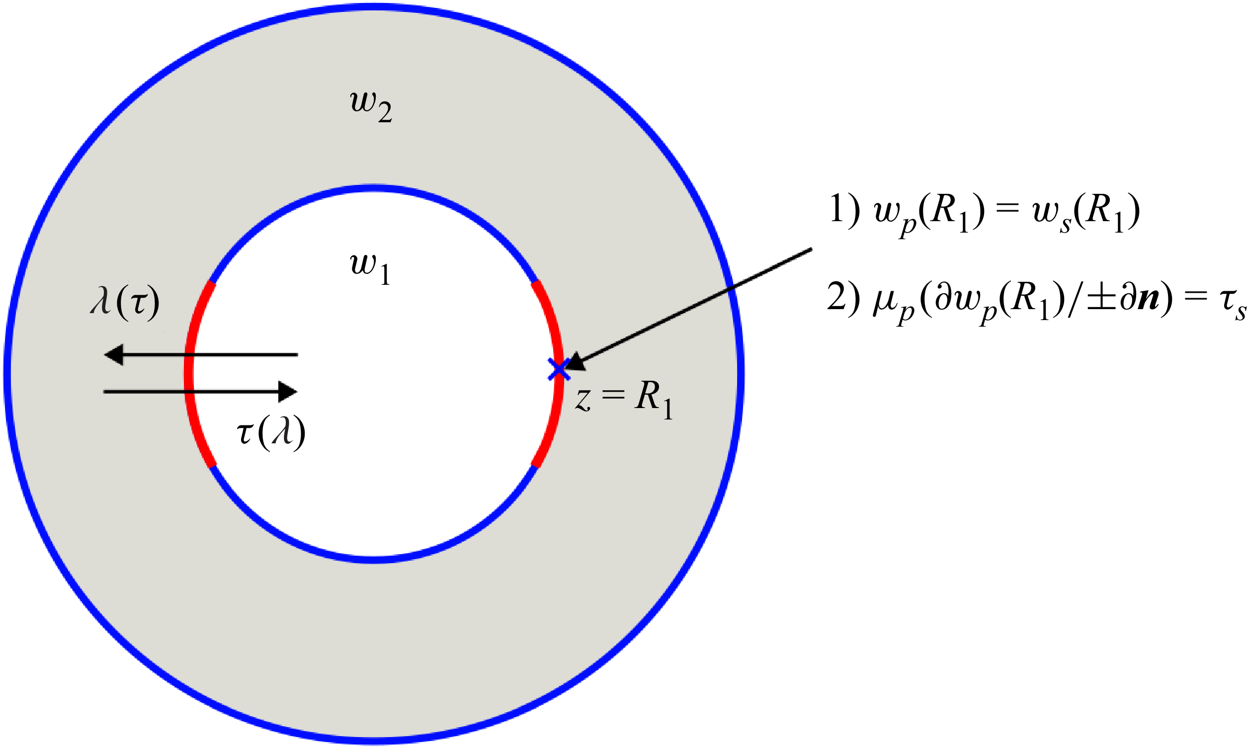


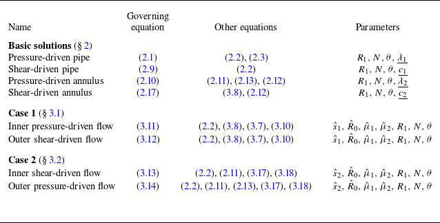


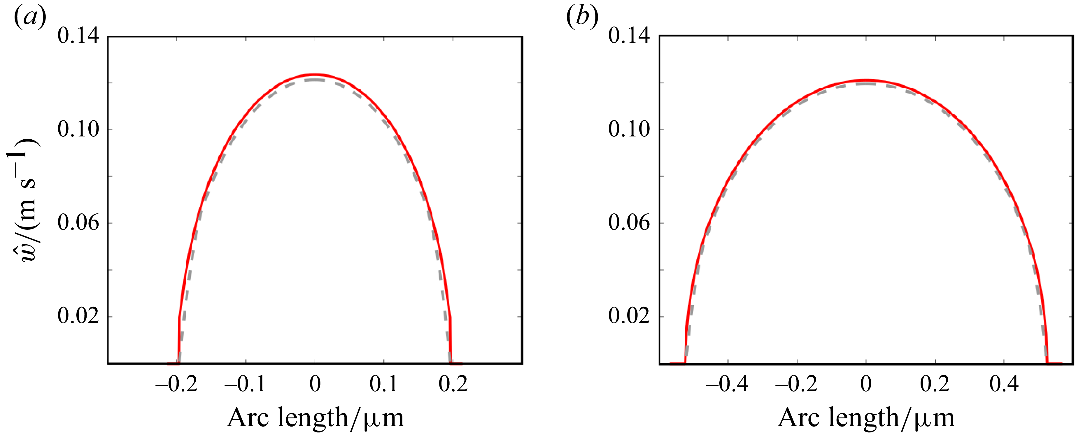

 Open access

