


1. Introduction
One of the most important effects of compressibility on high-speed flows manifests through flow–thermodynamics interactions. The wave nature of pressure at high Mach numbers leads to the emergence of a dilatational component of the velocity field and net pressure-work (pressure-dilatation covariance), both of which are absent at low speeds. The pressure-work transfers energy between dilatational kinetic and internal forms depending on the local state of flow expansion or contraction. The advent of these two energy components profoundly affects stability, transition and turbulence in the high-speed flows. The goal of this study is to advance the fundamental understanding of perturbation evolution in high-speed boundary layers by investigating flow–thermodynamics interactions at different Mach numbers.
The stability of compressible boundary layer flows (Lees & Lin Reference Lees and Lin1946; Mack Reference Mack1984; Reed, Saric & Arnal Reference Reed, Saric and Arnal1996; Criminale, Jackson & Joslin Reference Criminale, Jackson and Joslin2018) has been studied extensively using linear stability analysis. Lees & Lin (Reference Lees and Lin1946) established the necessary criteria for inviscid stability of compressible boundary layer flows. They conclude that an extremum of angular momentum ( $D(\bar {\rho }D\bar {U})=0$) is necessary for inviscid instability. A more complete understanding of compressible boundary layer stability was developed in the seminal work of Mack (Reference Mack1984). The emergence of Tollmien–Schlichting (TS) waves at high $Re$ leads to instability in incompressible flows (Mack Reference Mack1984; Schmid & Henningson Reference Schmid and Henningson2001). Compressibility has a stabilizing effect on the TS waves (also known as first mode) at subsonic Mach numbers. In supersonic flows, oblique modes of the TS family are more unstable than their streamwise counterparts. In related studies of homogeneous shear flows, Kumar, Bertsch & Girimaji (Reference Kumar, Bertsch and Girimaji2014) have shown that the effective Mach numbers of streamwise modes are larger than those of oblique modes. Thus oblique modes experience significantly lesser compressibility effects. At high Mach numbers, a new family of instability modes coexists alongside the first mode. These additional modes are acoustic in nature and exist whenever there is a region of relative supersonic flow in the boundary layer (Mack Reference Mack1984). For a flat-plate boundary layer with adiabatic walls, the first of these additional modes, called the second mode, becomes the dominant instability above $M=4$. In general, wall cooling destabilizes the second mode while stabilizing the first mode (Mack Reference Mack1984, Reference Mack1993; Masad, Nayfeh & Al-Maaitah Reference Masad, Nayfeh and Al-Maaitah1992).
Gushchin & Fedorov (Reference Gushchin and Fedorov1990), Fedorov & Khokhlov (Reference Fedorov and Khokhlov2001, Reference Fedorov and Khokhlov2002) and Fedorov & Tumin (Reference Fedorov and Tumin2011) analyse the eigenspectrum and the receptivity of high-speed boundary layers. Their findings show that the second-mode instability occurs in a region where two modes of the discrete spectrum are synchronized. These discrete modes were categorized as fast and slow based on their asymptotic behaviour near the leading edge (Fedorov & Tumin Reference Fedorov and Tumin2011). The coupling between the fast and slow modes in the synchronization region leads to the branching of the discrete spectrum (Gushchin & Fedorov Reference Gushchin and Fedorov1990). The branching pattern of the discrete spectrum is dependent on the Mach number (Fedorov & Tumin Reference Fedorov and Tumin2011). Consequently, depending on the flow parameters, the second mode can be associated with the fast or slow mode. Although the eigenspectrum (Gushchin & Fedorov Reference Gushchin and Fedorov1990; Fedorov & Khokhlov Reference Fedorov and Khokhlov2001; Fedorov & Tumin Reference Fedorov and Tumin2011) and the growth/decay (Mack Reference Mack1975, Reference Mack1984) of boundary layer instabilities have been investigated extensively in the past, compressibility effects on the instability modes require further attention. In this paper, we seek to further our understanding by examining the role of flow–thermodynamics interactions on the observed modal behaviour.
To examine compressibility effects, Kovasznay (Reference Kovasznay1953) proposes a decomposition of the fluctuating field into vorticity, entropy and acoustic components. The Kovasznay decomposition is dynamic in nature (Sagaut & Cambon Reference Sagaut and Cambon2008) and is valid only in the limit of small perturbations. The momentum potential theory (MPT) of Doak (Reference Doak1989) decomposes the momentum field ( $\rho \boldsymbol {u}$) into vortical, acoustic and thermal components. Jenvey (Reference Jenvey1989) extended MPT to identify the acoustic components of the fluctuating enthalpy and internal energy. The extended formulation is applied to study the net sound power output and the associated coupling between the irrotational and solenoidal fields at the boundary of stationary flows. Unnikrishnan & Gaitonde (Reference Unnikrishnan and Gaitonde2019) apply MPT to examine the contribution of the three components to the hypersonic boundary layer transition process. Their findings suggest that the vortical content of the momentum vector is of a similar magnitude for both first and second modes. Moreover, and perhaps more surprisingly, they find that vortical (momentum) fluctuations contain most of the disturbance energy even in the second mode, which is traditionally understood as being acoustic in nature (Mack Reference Mack1984). Recent investigations of high-speed boundary layer transition have revealed that the behaviour of aerodynamic heating depends on the underlying instability mechanism (Franko & Lele Reference Franko and Lele2013; Zhu et al. Reference Zhu, Lee, Chen, Wu, Chen and Gad-el Hak2018). For first-mode induced transition, generation of streamwise vortices leads to a strong overshoot of heat transfer at the end of the transition region. On the other hand, in numerical and experimental investigations (Franko & Lele Reference Franko and Lele2013; Zhu et al. Reference Zhu, Lee, Chen, Wu, Chen and Gad-el Hak2018) of second-mode induced transition, a stronger peak of surface temperature (denoted as HS) appears in the region of second-mode instability. Zhu et al. (Reference Zhu, Lee, Chen, Wu, Chen and Gad-el Hak2018) have shown that the aerodynamic heating facilitated by pressure-dilatation leads to the HS peak. Clearly, the coupling generated due to pressure-dilatation is fundamentally different for both first and second modes, and further insight into the role and contribution of various components of compressible velocity field will be of much value.
The Helmholtz decomposition of the flow field is better suited for examining dilatational kinetic and internal energy effects arising from compressibility. This static decomposition (Sagaut & Cambon Reference Sagaut and Cambon2008) can be applied to a broad set of vector fields and is not restricted to small fluctuations, unlike the Kovasznay decomposition. More importantly, the decomposition allows us to separate pure dilatational and vortical effects. The dilatational effects are fundamental in understanding the dynamic coupling between the flow and thermodynamic variables. Consequently, the Helmholtz decomposition has been used extensively to study compressibility effects in isotropic turbulence (Sarkar et al. Reference Sarkar, Erlebacher, Hussaini and Kreiss1991; Jagannathan & Donzis Reference Jagannathan and Donzis2016), wall-bounded turbulence (Yu, Xu & Pirozzoli Reference Yu, Xu and Pirozzoli2019) and turbulent boundary layer flows (Xu et al. Reference Xu, Wang, Wan, Yu, Li and Chen2021).
Following previous works in compressible turbulence, we apply the Helmholtz decomposition in the context of linear theory to examine the compressibility effects on boundary layer instability modes. An analytical formulation to examine the eigenmodes using Helmholtz decomposition is developed. We extend the decomposition of velocity to partition the pressure fluctuations into solenoidal and dilatational contributions. The compressibility effects at high Mach numbers on both first and second modes are analysed. The solenoidal and dilatational energy levels of the instability modes are established. Finally, the decomposition is applied to the key turbulence processes to explicate the observed instability behaviour.
2. Linear analysis and Helmholtz decomposition
The governing equations for an ideal compressible fluid are
 $$\begin{gather} \frac{\partial \rho^{{\dagger}}}{\partial t^{{\dagger}}} + \frac{\partial}{\partial x_j^{{\dagger}}} (\rho^{{\dagger}} u_j^{{\dagger}}) = 0, \end{gather}$$
 $$\begin{gather}\frac{ \partial (\rho^{{\dagger}} u_i^{{\dagger}})}{\partial t^{{\dagger}}} + \frac{\partial (\rho^{{\dagger}} u_i^{{\dagger}} u_j^{{\dagger}})}{\partial x_j^{{\dagger}}} =-\frac{\partial p^{{\dagger}}}{\partial x_i^{{\dagger}}} + \frac{\partial \tau_{ij}^{{\dagger}}}{\partial x_j^{{\dagger}}}, \end{gather}$$
 $$\begin{gather}\frac{\partial}{\partial t^{{\dagger}}} \left(\frac{p^{{\dagger}}}{\gamma-1}\right) + \frac{\partial }{\partial x_j^{{\dagger}}}\left(\frac{p^{{\dagger}} u_j^{{\dagger}}}{\gamma-1}\right) = \frac{\partial}{\partial x_j^{{\dagger}}} \left( \kappa^{{\dagger}}\,\frac{\partial T^{{\dagger}}}{\partial x_j^{{\dagger}}} \right) - p^{{\dagger}}\,\frac{\partial u_k^{{\dagger}}}{\partial x_k^{{\dagger}}} + \tau_{ij}^{{\dagger}}\,\frac{\partial u_i^{{\dagger}}}{\partial x_j^{{\dagger}}}, \end{gather}$$
 $$\begin{gather}p^{{\dagger}}= \rho^{{\dagger}} R T^{{\dagger}}, \end{gather}$$
where the superscript  ${{{\dagger}} }$ is used to denote the dimensional variables. The density of the fluid is denoted by $\rho ^{{\dagger}}$, velocity by $u_i^{{\dagger}}$, temperature by $T^{{\dagger}}$, and pressure by $p^{{\dagger}}$. Also, $\gamma$ is the specific heat ratio, $\kappa ^{{\dagger}}$ is the coefficient of thermal conductivity, and $\tau _{ij}^{{\dagger}}$ is the viscous stress tensor given by
 \begin{equation} \tau_{ij}^{{\dagger}}=\mu^{{\dagger}}\left(\frac{\partial u_i^{{\dagger}}}{\partial x_j^{{\dagger}}}+\frac{\partial u_j^{{\dagger}}}{\partial x_i^{{\dagger}}}\right)-\frac{2}{3}\,\mu^{{\dagger}}\,\frac{\partial u_k^{{\dagger}}}{\partial x_k^{{\dagger}}}\,\delta_{ij}. \end{equation}
The coefficient of viscosity  $\mu ^{{\dagger}}$ is dependent on the local temperature as dictated by the Sutherland's law (Sutherland Reference Sutherland1893).
Restricting consideration to a boundary layer, the dimensional variables  $\rho ^{{\dagger}}$, $u_i^{{\dagger}}$ and $T^{{\dagger}}$ are normalized by their respective freestream values $\rho _\infty$, $U_\infty$ and $T_\infty$. Pressure ( $p^{{\dagger}}$) is normalized by the freestream dynamic pressure $\rho _\infty U_\infty ^2$. The Blasius length scale $L_r=\sqrt {\mu _\infty x^{{\dagger}} /\rho _\infty U_\infty }$ is used to normalize the spatial coordinate $x_i^{{\dagger}}$. The fluid properties $\mu ^{{\dagger}}$ and $\kappa ^{{\dagger}}$ are also normalized by the freestream values $\kappa _\infty$ and $\mu _\infty$, respectively. The non-dimensional forms of the compressible Navier–Stokes equations are then obtained as
 $$\begin{gather} \frac{\partial \rho}{\partial t} + \frac{\partial}{\partial x_j} (\rho u_j) = 0, \end{gather}$$
 $$\begin{gather}\frac{ \partial (\rho u_i)}{\partial t} + \frac{\partial (\rho u_i u_j)}{\partial x_j} =-\frac{\partial p}{\partial x_i} + \frac{1}{Re}\,\frac{\partial \tau_{ij}}{\partial x_j}, \end{gather}$$
 $$\begin{gather}\frac{\partial p}{\partial t} + \frac{\partial }{\partial x_j}\left(\,pu_j\right) = \frac{1}{M^2\,Re\,Pr}\,\frac{\partial}{\partial x_j} \left( \kappa\,\frac{\partial T}{\partial x_j} \right) - (\gamma-1)p\,\frac{\partial u_k}{\partial x_k} + \frac{\gamma-1}{Re}\,\tau_{ij}\,\frac{\partial u_i}{\partial x_j}, \end{gather}$$
 $$\begin{gather}p = \frac{1}{\gamma M^2}\,\rho T. \end{gather}$$
The non-dimensional parameters in the governing equations (2.3) are
 \begin{equation} Re=\frac{\rho_\infty U_\infty L_r}{\mu_\infty},\quad M=\frac{U_\infty}{\sqrt{\gamma R T_\infty}},\quad Pr=\frac{\mu_\infty C_p}{\kappa_\infty}, \end{equation}
where  $C_P=\gamma R/(\gamma -1)$ is the specific heat at constant pressure.
For linear stability analysis, the flow variables are decomposed into a basic state and perturbations:
 \begin{equation} A=\bar{A}+A'. \end{equation}
Here,  $A$ represents the flow and thermodynamic variables ( $u_i, \rho, p, T$). The fluid properties, viscosity ( $\mu$) and thermal conductivity ( $\kappa$), are also decomposed into a base state and perturbations. The basic state for a flat-plate boundary layer flow is taken to be two-dimensional and locally parallel. As a result, the base variables vary only along the wall-normal direction $y$. The basic state is obtained by solving the two-dimensional compressible laminar boundary layer equations with adiabatic walls using the Levy–Lees similarity transformation (Rogers Reference Rogers1992). The perturbation equations in the linear limit are (Malik Reference Malik1990)
 $$\begin{gather} \frac{\partial \rho'}{\partial t} + \bar{U}_i\,\frac{\partial \rho'}{\partial x_i} +\frac{\partial \bar{\rho}}{\partial x_i}\,u_i' + \bar{\rho}\,\frac{\partial u_i'}{\partial x_i} = 0, \end{gather}$$
 $$\begin{gather}\bar{\rho}\,\frac{\partial u_i'}{\partial t} + \bar{\rho}\bar{U}_k\,\frac{\partial u_i'}{\partial x_k} +\bar{\rho}\,\frac{\partial \bar{U}_i}{\partial x_k}\,u_k' =-\frac{\partial p'}{\partial x_i} +\frac{1}{Re}\,\frac{\partial \tau_{ik}'}{\partial x_k}, \end{gather}$$
 \begin{gather} \bar{\rho}\,\frac{\partial T'}{\partial t} + \bar{\rho}\bar{U}_i\,\frac{\partial T'}{\partial x_i} + \bar{\rho}u_i'\,\frac{\partial \bar{T}}{\partial x_i} = (\gamma-1)M^2\left[\frac{\partial p'}{\partial t}+\bar{U}_i\,\frac{\partial p'}{\partial x_i}\right] - \frac{1}{Re\,Pr}\,\frac{\partial q_k'}{\partial x_k}\nonumber\\ \qquad\qquad\qquad\qquad\qquad\qquad +\, \frac{(\gamma-1)M^2}{Re}\left[\tau_{ij}'\,\frac{\partial \bar{U}_i}{\partial x_j} + \bar{\tau}_{ij}\,\frac{\partial u_i'}{\partial x_j}\right], \end{gather}
 \begin{gather} p' = \frac{1}{\gamma M^2}\left(\bar{\rho} T'+ \rho' \bar{T}\right), \end{gather}
where  $\tau _{ik}'$ is the linearized viscous stress tensor, and $q_k'$ is the perturbation thermal conduction term. The components of the linearized viscous stress tensor $\tau _{ik}'$ and thermal conduction term $q_k'$ are given by
 \begin{equation} \left.\begin{gathered} \tau_{ik}'= \bar{\mu}\left(\frac{\partial u_i'}{\partial x_k}+\frac{\partial u_k'}{\partial x_i}\right)+\mu'\left(\frac{\partial \bar{U}_i}{\partial x_k}+\frac{\partial \bar{U}_k}{\partial x_i}\right)+\bar{\lambda}\,\frac{\partial u_k'}{\partial x_k}\,\delta_{ik}, \\ q_k'=-\bar{\kappa}\,\frac{\partial T'}{\partial x_k}-\kappa'\,\frac{{\rm d}\bar{T}}{{\rm d}x_k}. \end{gathered}\right\} \end{equation}
We consider a normal mode for the perturbations  $A'$ (Mack Reference Mack1984) of the form
 \begin{equation} A'=\hat{A}(y)\exp({\iota(\alpha x+\beta z-\omega t)}), \end{equation}
where  $\alpha$ and $\beta$ are the wavenumbers in the streamwise and spanwise directions, $\omega$ is the temporal frequency, and $\hat {A}$ is the perturbation amplitude varying in the wall-normal direction. For temporal stability analysis, $\alpha$ and $\beta$ are real and specified a priori, while $\omega$ is the complex eigenvalue obtained from analysis. The sign of the imaginary part of $\omega$ ( $\omega _i$) determines the stability: perturbations grow if $\omega _i>0$, and decay if $\omega _i<0$. The modal form of perturbations is substituted into the linearized perturbation equation (2.6) to formulate the eigenvalue problem
 \begin{equation} \omega\varTheta =\boldsymbol{A}^{-1}\boldsymbol{B}(\alpha,\beta,Re,M,Pr)\,\varTheta. \end{equation}
Here,  $\varTheta =[\hat {u},\hat {v},\hat {w},\hat {T},\hat {p}]$ are the eigenmode shapes corresponding to the eigenvalue $\omega$. The elements of the fifth-order coefficient matrices $\boldsymbol {A}$ and $\boldsymbol {B}$ are listed in Sharma & Girimaji (Reference Sharma and Girimaji2022). No-slip and zero thermal perturbation boundary conditions are used for velocity and temperature, while a Neumann boundary condition for pressure is obtained by solving the wall-normal momentum equation (2.6b).
2.1. Modal Helmholtz decomposition
The Helmholtz decomposition allows any three-dimensional vector field to be expressed as a sum of solenoidal and dilatational components. Following the fundamental theorem of vector calculus (Murray Reference Murray1898), the perturbation velocity vector  $\boldsymbol {u}'$ is cast as
 \begin{equation} \boldsymbol{u}'=\boldsymbol{u}'^s+\boldsymbol{u}'^d,\quad \boldsymbol{u}'^s=\boldsymbol{\nabla} \times \boldsymbol{\varPsi},\quad \boldsymbol{u}'^d=\boldsymbol{\nabla} \phi. \end{equation}
Here,  $\phi$ is the velocity potential, and $\boldsymbol {\varPsi }$ is the vector potential. The solenoidal velocity $\boldsymbol {u}'^s$ is divergence-free, and the dilatational part $\boldsymbol {u}'^d$ is irrotational by definition. The potentials $\phi$ and $\boldsymbol {\varPsi }$ are governed by the Poisson equations (Hirasaki & Hellums Reference Hirasaki and Hellums1970)
 \begin{equation} \nabla^2\phi=\boldsymbol{\nabla}\boldsymbol{\cdot}\boldsymbol{u}', \quad\nabla^2\boldsymbol{\varPsi}=-\boldsymbol{\nabla}\times\boldsymbol{u}'. \end{equation}
It is worth noting that the vector potential  $\boldsymbol {\varPsi }$ is constrained to be solenoidal (Hirasaki & Hellums Reference Hirasaki and Hellums1970). The boundary conditions given by
 \begin{equation} \left.\frac{\partial \phi}{\partial y}\right|_{0,l_y}=0,\quad \left.\varPsi_x\right|_{0,l_y}=0,\quad\left.\frac{\partial \varPsi_y}{\partial y}\right|_{0,l_y}=0,\quad \left.\varPsi_z\right|_{0,l_y}=0 \end{equation}
must be satisfied at the wall and the freestream boundary for a unique vector potential (Hirasaki & Hellums Reference Hirasaki and Hellums1970). Here,  $\varPsi _x$, $\varPsi _y$ and $\varPsi _z$ are the streamwise, wall-normal and spanwise components of the vector potential, respectively.
As mentioned in the Introduction, we use Helmholtz decomposition in conjunction with linear stability analysis to gain further insight into the compressibility effects on compressible boundary layer stability. The velocity field of each eigenmode is subjected to Helmholtz decomposition. The potentials  $\phi$ and $\boldsymbol {\varPsi }$ are expressed in the normal mode form as
 \begin{equation} \phi=\hat{\phi}(y)\exp({\iota(\alpha x+\beta z-\omega t)}),\quad \varPsi_i=\hat{\varPsi}_i(y)\exp({\iota(\alpha x+\beta z-\omega t)}), \end{equation}
where  $\hat {\phi }$ and $\hat {\varPsi }_i$ are the eigenfunctions of the velocity and vector potentials, respectively. Substituting the normal mode form of potentials (2.13a,b) in the Poisson equations (2.11a,b), the governing equations for the potential eigenfunctions are obtained:
 \begin{equation} \left.\begin{gathered} -\alpha^2\hat{\phi}+\frac{{\rm d}^2\hat{\phi}}{{{\rm d} y}^2}-\beta^2\hat{\phi}= \iota\alpha\hat{u}+\frac{{\rm d}\hat{v}}{{\rm d} y}+\iota\beta\hat{w}, \\ -\alpha^2\hat{\varPsi}_x+\frac{{\rm d}^2\hat{\varPsi}_x}{{{\rm d} y}^2}-\beta^2 \hat{\varPsi}_x=\iota\beta\hat{v}-\frac{{\rm d}\hat{w}}{{\rm d} y}, \\ -\alpha^2\hat{\varPsi}_y+\frac{{\rm d}^2\hat{\varPsi}_y}{{{\rm d} y}^2}-\beta^2\hat{\varPsi}_y= \iota\alpha\hat{w}-\iota\beta\hat{u}, \\ -\alpha^2\hat{\varPsi}_z+\frac{{\rm d}^2\hat{\varPsi}_z}{{{\rm d} y}^2}-\beta^2\hat{\varPsi}_z= \frac{{\rm d}\hat{u}}{{\rm d} y}-\iota\alpha\hat{v}. \end{gathered}\right\} \end{equation}
Here,  $\hat {u}$, $\hat {v}$ and $\hat {w}$ are the eigenmode shapes of the streamwise, wall-normal and spanwise velocity components, respectively. The following boundary conditions must be satisfied for uniqueness of the potentials:
 \begin{equation} \left.\frac{{\rm d} \hat{\phi}}{{\rm d} y}\right|_{0,l_y}=0,\quad \left.\hat{\varPsi}_x\right|_{0,l_y}=0,\quad\left.\frac{{\rm d} \hat{\varPsi}_y}{{\rm d} y}\right|_{0,l_y}=0,\quad \left.\hat{\varPsi}_z\right|_{0,l_y}=0. \end{equation}
A more detailed discussion on the boundary conditions is provided in Appendix A.
The solenoidal and dilatational parts of the velocity field can also be expressed in the modal form
 \begin{equation} u'^s_i=\hat{u}^s_i(y)\exp({\iota(\alpha x+\beta z-\omega t)}),\quad u'^d_i=\hat{u}^d_i(y)\exp({\iota(\alpha x+\beta z-\omega t)}). \end{equation}
The eigenfunctions  $\hat {u}^s_i$ and $\hat {u}^d_i$ are then obtained using
 \begin{equation} \left.\begin{gathered} \hat{u}^d =\iota\alpha\hat{\phi},\quad\hat{v}^d=\frac{{\rm d}\hat{\phi}}{{\rm d}y}, \quad\hat{w}^d=\iota\beta\hat{\phi}, \\ \hat{u}^s =\frac{{\rm d}\hat{\varPsi}_z}{{\rm d} y}-\iota\beta\hat{\varPsi}_y, \quad \hat{v}^s=\iota\beta\hat{\varPsi}_x-\iota\alpha\hat{\varPsi}_z, \quad \hat{w}^s=\iota\alpha\hat{\varPsi}_y-\frac{{\rm d}\hat{\varPsi}_x}{{\rm d}y}. \end{gathered}\right\} \end{equation}
The fluctuating velocity eigenfunctions can be recovered from  $\hat {u}_i^s$ and $\hat {u}_i^d$:
 \begin{equation} \hat{u}_i=\hat{u}_i^s+\hat{u}_i^d. \end{equation}
2.1.1. Momentum decomposition
In this work, we employ Helmholtz decomposition to partition the momentum perturbations ( $m_i'$) as well. The momentum perturbations in the linear limit can be approximated as
 \begin{equation} m_i'=\rho u_i-\overline{\rho u}=\bar{\rho}u_i'+\rho'\bar{U}_i. \end{equation}
The momentum perturbations are then split into solenoidal and dilatational parts:
 \begin{equation} m_i'=m_i'^s+m_i'^d, \end{equation}
where  $m_i'^s$ is the solenoidal component and $m_i'^d$ is the dilatational component of the momentum field. The eigenfunctions of $m_i'^s$ and $m_i'^d$ can also be obtained by following the procedure outlined in (2.14)–(2.17).
2.2. Pressure decomposition
The decomposition of pressure in general is not unique, and multiple formulations exist. Erlebacher et al. (Reference Erlebacher, Hussaini, Kreiss and Sarkar1990) define the solenoidal pressure as the field that satisfies the incompressible Poisson equation with a source term corresponding to the solenoidal velocity. Then the dilatational pressure is defined as the difference between the total pressure and the solenoidal pressure. More recently, Yu, Xu & Pirozzoli (Reference Yu, Xu and Pirozzoli2020) proposed a formal partition of pressure into the rapid, slow, viscous and mass flux related terms. The rapid and slow terms can be further split into solenoidal and dilatational parts using the Helmholtz decomposition of velocity. Building on the momentum potential theory approach (Doak Reference Doak1989), Unnikrishnan & Gaitonde (Reference Unnikrishnan and Gaitonde2020) also propose a split of pressure fluctuations into their hydrodynamic, acoustic and entropic components. In this subsection, a novel formulation to decompose the total pressure fluctuations into solenoidal ( $p'^s$) and dilatational ( $p'^d$) pressure in the linear limit is presented.
The divergence of the linearized perturbation momentum equation (2.6b) yields the following equation for pressure perturbations:
 \begin{align} -\frac{\partial^2 p'}{\partial x_i\,\partial x_i}+\frac{1}{\bar{\rho}}\,\frac{\partial \bar{\rho}}{\partial x_i}\,\frac{\partial p'}{\partial x_i}&= \left[\bar{\rho}\,\frac{\partial}{\partial t}+\bar{\rho}\bar{U}_k\,\frac{\partial}{\partial x_k}\right]\frac{\partial u_i'}{\partial x_i}+2\bar{\rho}\,\frac{\partial\bar{U}_k}{\partial x_i}\,\frac{\partial u_i'}{\partial x_k}\nonumber\\ &\quad -\frac{1}{Re}\left[\frac{\partial^2\tau_{ik}'}{\partial x_i\,\partial x_k}-\frac{1}{\bar{\rho}}\,\frac{\partial \bar{\rho}}{\partial x_i}\,\frac{\partial \tau_{ik}'}{\partial x_k}\right]. \end{align}
The Helmholtz decomposition of the velocity field  $u_i'=u_i'^s+u_i'^d$ is substituted in (2.21). We assume that the evolution of $p'^s$ is determined completely by the solenoidal part of velocity field. The governing equation for the solenoidal pressure is
 \begin{equation} -\frac{\partial^2 p'^s}{\partial x_i\,\partial x_i}+\frac{1}{\bar{\rho}}\,\frac{\partial \bar{\rho}}{\partial x_i}\,\frac{\partial p'^s}{\partial x_i} = 2\bar{\rho}\,\frac{\partial\bar{U}_k}{\partial x_i}\,\frac{\partial u_i'^s}{\partial x_k} -\frac{1}{Re}\left[\frac{\partial^2\tau_{ik}'^s}{\partial x_i\,\partial x_k}-\frac{1}{\bar{\rho}}\,\frac{\partial \bar{\rho}}{\partial x_i}\,\frac{\partial \tau_{ik}'^s}{\partial x_k}\right]. \end{equation}
The components of the solenoidal viscous stress tensor  $\tau _{ik}'^s$ are
 \begin{equation} \tau_{ik}'^s=\bar{\mu}\left(\frac{\partial u_i'^s}{\partial x_k}+\frac{\partial u_k'^s}{\partial x_i}\right). \end{equation}
The solenoidal pressure satisfies the following Neumann boundary condition at the wall and the freestream boundary:
 \begin{equation} \left.\frac{\partial p'^s}{\partial y}\right|_{(0,l_y)}=\frac{1}{Re}\,\frac{\partial \tau_{2k}'^s}{\partial x_k} . \end{equation}
It must be noted that in the absence of gradient of mean density and temperature,  $p'^s$ is governed by the incompressible Poisson equation. Thus for a constant base density and temperature profile, the current decomposition of pressure reduces to the formulation presented in Erlebacher et al. (Reference Erlebacher, Hussaini, Kreiss and Sarkar1990).
The dilatational pressure can then be computed by subtracting  $p'^s$ from the total pressure fluctuations $p'$:
$p'$:
 \begin{equation} p'^d=p'-p'^s. \end{equation}
 The pressure decomposition proposed is also applied to each eigenmode. Thus,  $p'^s$ and $p'^d$ are expressed in the modal form
 \begin{equation} p'^s=\hat{p}^s(y)\exp({\iota(\alpha x+\beta z-\omega t)}),\quad p'^d=\hat{p}^d(y)\exp({\iota(\alpha x+\beta z-\omega t)}). \end{equation}
The modal form of pressure perturbations is substituted in (2.22) to obtain the following second-order ordinary differential equation (ODE) for  $\hat {p}^s$:
 \begin{equation} \frac{{\rm d}^2\hat{p}^s}{{{\rm d}y}^2}-\left[\frac{1}{\bar{\rho}}\,\frac{{\rm d}\bar{\rho}}{{\rm d} y}\right]\frac{{\rm d}\hat{p}^s}{{\rm d}y}-(\alpha^2+\beta^2)\hat{p}^s=-\hat{\mathcal{S}}(\hat{u}_i^s;\bar{\rho},\bar{U},\bar{\mu}), \end{equation}
where  $\hat {\mathcal {S}}(\hat {u}_i^s;\bar {\rho },\bar {U},\bar {\mu })$ is the source term dependent on the solenoidal velocity eigenfunction and the basic state
 \begin{equation} \hat{\mathcal{S}}=2\iota\alpha\bar{\rho}\,\frac{{\rm d}\bar{U}}{{\rm d} y}\,\hat{v}^s -\frac{1}{Re}\left[2\,\frac{{\rm d}^2\bar{\mu}}{{{\rm d} y}^2}-\frac{2}{\bar{\rho}}\,\frac{{\rm d}\bar{\rho}}{{\rm d} y}\,\frac{{\rm d}\bar{\mu}}{{\rm d} y}\right]\frac{{\rm d}\hat{v}^s}{{\rm d}y}-\frac{1}{Re}\left[2\,\frac{{\rm d}\bar{\mu}}{{\rm d} y}-\frac{\bar{\mu}}{\bar{\rho}}\,\frac{{\rm d}\bar{\rho}}{{\rm d} y}\right]\hat{\nabla}^2\hat{v}^s . \end{equation}
Here,  $\hat {\nabla }^2\hat {v}^s=-(\alpha ^2+\beta ^2)\hat {v}^s+\textrm {d}^2\hat {v}^s/{\textrm {d} y}^2$ denotes the Laplacian of $\hat {v}^s$. The solenoidal component of pressure eigenmode is obtained by solving the ODE (2.22) alongside the boundary condition
 \begin{equation} \frac{{\rm d}\hat{p}^s}{{\rm d} y}=\frac{1}{Re}\left[\bar{\mu}\,\hat{\nabla}^2\hat{v}^s+\frac{{\rm d}\bar{\mu}}{{\rm d} y}\,\frac{{\rm d}\hat{v}^s}{{\rm d} y}\right]. \end{equation}
In high-speed flows, the velocity field develops a dilatational component allowing for pressure to perform work on the velocity field. The kinetic energy can therefore be diverted to internal energy via the pressure-dilatation mechanism (Sarkar Reference Sarkar1992; Mittal & Girimaji Reference Mittal and Girimaji2019). Thus, in dealing with compressible flows, it is important to consider flow–thermodynamic interactions and account for both kinetic and internal energy. In the linear limit, the perturbation kinetic energy contained in the velocity fluctuations and the internal energy in pressure fluctuations (Mittal & Girimaji Reference Mittal and Girimaji2019) are defined as
 \begin{equation} k=\frac{1}{2}\,\bar{\rho}u_i'u_i',\quad e=\frac{p'p'}{2\gamma\bar{P}}. \end{equation}
The fluctuating kinetic energy can be partitioned into three components using the Helmholtz decomposition of the velocity field:
 \begin{equation} k=\underbrace{\tfrac{1}{2}\bar{\rho}u_i'^su_i'^s}_{k_s}+\underbrace{\tfrac{1}{2}\bar{\rho}u_i'^du_i'^d}_{k_d}+\underbrace{ \bar{\rho}u_i'^su_i'^d}_{k_{sd}}, \end{equation}
where  $k_s$, $k_d$ and $k_{sd}$ are the solenoidal, dilatational and covariance components of kinetic energy, respectively. Here, $k_s$ and $k_d$ quantify the energy in the solenoidal and dilatational velocity field, and are always positive; $k_{sd}$ represents the correlation between the solenoidal and dilatational velocity field, and is not positive definite. Similarly, the internal energy in pressure fluctuations can also be decomposed into solenoidal ( $e_s$), dilatational ( $e_d$) and covariance ( $e_{sd}$) components:
 \begin{equation} e=\underbrace{\frac{p'^sp'^s}{2\gamma\bar{P}}}_{e_s}+\underbrace{\frac{p'^dp'^d}{2\gamma\bar{P}}}_{e_d}+\underbrace{\frac{p'^sp'^d}{\gamma\bar{P}}}_{e_{sd}}. \end{equation}
2.3. Numerical methodology
The eigenmodes are computed by solving the global eigenvalue problem (2.9) on  $N=199$ collocation points using Chebyshev polynomials (Malik Reference Malik1990). The Chebyshev polynomials are defined on the following Gauss–Labato points ( $\xi _i$) in the interval $[-1,1]$:
 \begin{equation} \xi_i=\cos{\frac{{\rm \pi} i}{N}},\quad i=0,1,\ldots, N. \end{equation}
The physical domain ( $y \in [0,l_{y}]$) is mapped to the computational domain using an algebraic stretching function (Malik Reference Malik1990)
 \begin{equation} y=a\,\frac{1+\xi}{b-\xi},\quad\mbox{where } b=1+\frac{2a}{l_{y}}\mbox{ and } a=\frac{y_ll_{y}}{l_{y}-2y_l}. \end{equation}
Here,  $l_{y}$ is the length of the physical domain, and the parameter $y_l$ is set equal to half of the 99 % boundary layer thickness ( $y_{99}$) in all stability calculations.
For each eigenmode, the boundary value problem (2.14)–(2.15a–d) is solved to compute the potential eigenfunctions  $\hat {\phi }$ and $\hat {\varPsi }_i$. The second-order ODE (2.14) is discretized using Chebyshev polynomials in the wall-normal direction. The mode shapes for the solenoidal and dilatational parts of velocity are then obtained from (2.17). Subsequently, the ODE (2.27) is also solved using Chebyshev polynomials to compute $\hat {p}^s$. The mode shape of the dilatational pressure $\hat {p}^d$ is then obtained from the residual of $\hat {p}$ and $\hat {p}^s$.
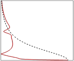
To verify the accuracy of the modal formulation of Helmholtz decomposition, the velocity eigenfunctions obtained from (2.18) are compared against the standard velocity eigenfunctions obtained from (2.9). The mode shapes for the streamwise and wall-normal velocity at  $M=6$ and $Re=4000$ obtained from the two approaches are shown in figure 1. The mode shapes correspond to the most unstable eigenmode at $\alpha =0.175$ and $\beta =0$. The sum total of the solenoidal and dilatational velocity recovers the velocity mode shapes obtained from the standard eigenmode analysis. The profiles of the velocity divergence ( $\boldsymbol {\nabla }\boldsymbol {\cdot }\boldsymbol {u}'$) and vorticity magnitude ( $|\boldsymbol {\varOmega }|=|\boldsymbol {\nabla }\times \boldsymbol {u}'|$) are presented in figure 2. It is evident from the figures that the solenoidal part of the velocity field is divergence-free as the dilatational component contributes to all of the dilatation in the flow. Similarly, $\boldsymbol {u}'^d$ is irrotational, and vorticity is entirely contained in the solenoidal mode. It is worth noting that the solenoidal field does not include acoustic waves and is entirely vortical in nature. The dilatational field, on the other hand, is not restricted to acoustic phenomena and incorporates both acoustic and entropy effects (Sagaut & Cambon Reference Sagaut and Cambon2008).
Mode shapes of (a) streamwise velocity ( $\hat {u}$) and (b) wall-normal velocity ( $\hat {v}$), at $M=6$, $Re=4000$, $\alpha =0.175$ and $\beta =0$. Black solid lines correspond to the mode shapes obtained from the standard eigenmode formulation (2.9). Dashed red lines denote the sum total of the dilatational and solenoidal parts of the velocity.

Mode shapes of the (a) velocity divergence ( $\boldsymbol {\nabla }\boldsymbol {\cdot }\boldsymbol {u}'$) and (b) vorticity magnitude ( $|\boldsymbol {\varOmega }|=|\boldsymbol {\nabla }\times \boldsymbol {u}|$), at $M=6$, $Re=4000$, $\alpha =0.175$ and $\beta =0$. Red dashed lines correspond to the (a) divergence and (b) vorticity of the solenoidal velocity $\boldsymbol {u}'^s$. Blue dash-dotted lines represent the (a) divergence and (b) vorticity of the dilatational velocity $\boldsymbol {u}'^d$.

3. Solenoidal and dilatational field contributions to instability
In this section, we examine the contributions of solenoidal (vortical) and dilatational ( $\textrm {acoustic}+\textrm {entropy}$) velocity fields to the instability at different Mach numbers. The stability analysis is performed for $M\in [0.5,8]$ at fixed $Re=4000$ and $Pr=0.7$. The Reynolds number selected herein ( $Re=4000$) is greater than the minimum critical Reynolds number at all $M$. Moreover, analysis of lower Reynolds number cases indicates that the compressibility effects are not strongly influenced by $Re$. Therefore, we present only results corresponding to $Re=4000$ in this work. For a given Mach number, the most unstable mode is computed by performing a parameter sweep in the streamwise–spanwise $(\alpha,\beta )$ wavenumber space. The most unstable first mode is obtained for $M=\{0.5,1,2,3,4,6\}$, and the most unstable second mode is computed for $M=\{4,5,6,7,8\}$. It is worth noting that the second mode is stable for $M\leq 3$. The solenoidal and dilatational energy levels of an eigenmode are quantified by considering global averages as defined in Sharma & Girimaji (Reference Sharma and Girimaji2022). The global-averaged kinetic ( $k^g$) and internal energy ( $e^g$) are obtained by integrating the amplitude of velocity and pressure perturbations in the wall-normal direction:
 \begin{equation} k^g = \frac{1}{l_{y}}\int_0^{l_{y}}\frac{\bar{\rho}\hat{u}_i\hat{u}_i^*}{2}\,{{\rm d} y},\quad e^g = \frac{1}{l_{y}}\int_0^{l_{y}}\frac{\hat{p}\hat{p}^*}{2\gamma\bar{P}}\,{{\rm d} y}, \end{equation}
where  $\hat {u}_i^*$ denotes the complex conjugate of $\hat {u}_i$. The global-averaged kinetic energy can be split into the solenoidal kinetic energy ( $k_s^g$), dilatational kinetic energy ( $k_d^g$) and covariance ( $k_{sd}^g$) components. The averaged energy components are defined as
 \begin{equation} \left.\begin{gathered} k_s^g = \frac{1}{2l_{y}}\int_0^{l_{y}}\bar{\rho}\hat{u}_i^s(\hat{u}_i^s)^* \,{{\rm d} y},\\ k_d^g = \frac{1}{2l_{y}}\int_0^{l_{y}}\bar{\rho}\hat{u}_i^d(\hat{u}_i^d)^* \,{{\rm d} y},\\ k_{sd}^g = \frac{1}{2l_{y}}\int_0^{l_{y}}\left(\bar{\rho}\hat{u}_i^s(\hat{u}_i^d)^*+ \bar{\rho}\hat{u}_i^d (\hat{u}_i^s)^*\right){\rm d} y. \end{gathered}\right\} \end{equation}
3.1. Most unstable first and second modes
The solenoidal and dilatational contributions to the most unstable first and second modes are considered now. The growth rates of the most unstable first and second modes at different  $M$ are shown in figure 3. The first mode is the dominant instability for $M<4$, while the second mode dominates at higher $M$. The most unstable first mode is oblique for $M\geqslant 1$, while the most unstable second mode is always streamwise. Figure 4 plots the solenoidal, dilatational and covariance energy fractions at different $M$ for both first and second modes. The first mode is purely solenoidal as the dilatational and covariance components have negligible energy. This is not surprising, as the first mode instability is a TS wave, which is a vortical instability. The second mode, on the other hand, is dominantly dilatational and has non-negligible solenoidal energy. The solenoidal energy fraction increases with Mach number. The dilatational and solenoidal modes are negatively correlated for the second mode. The covariance value is less than $-5\,\%$ for $M<6$, and gradually increases in magnitude up to $-15\,\%$ at $M=8$. The dominantly dilatational nature of the second mode indicates that flow–thermodynamic interactions are significant for the second mode. For the first mode, however, flow–thermodynamic interactions are not important as the dilatational velocity is negligible.
Growth rates ( $\omega _i$) of the most unstable first and second modes at different $M$.
$M$.

Solenoidal ( $k_s^g$), dilatational ( $k_d^g$) and covariance ( $k_{sd}^g$) components of the average kinetic energy for the most unstable (a) first mode and (b) second mode, at different $M$.
$M$.

The solenoidal and dilatational parts of the velocity eigenfunctions for the most unstable mode at  $M=0.5$ are shown in figure 5. The most unstable mode at $M=0.5$ is a streamwise first mode. The eigenfunctions are normalized by the magnitude of pressure perturbation at the wall. The dilatational velocity is negligible in both the streamwise and wall-normal directions as the first mode is a vortical instability. The streamwise solenoidal velocity has a strong peak near the critical layer ( $y_c=0.83$), while the wall-normal solenoidal velocity peaks near the boundary layer edge ( $y_{99}=4.95$). Figure 6 plots the eigenfunctions of the dilatational and solenoidal parts of velocity for the most unstable mode at $M=3$. The most unstable mode at $M=3$ is an oblique first mode. Much like the first mode at $M=0.5$, the dilatational contribution to the velocity field is negligible. The solenoidal part of the velocity dominates and has a strong peak near the critical layer ( $y_c=3.85$) in the streamwise and spanwise directions. The solenoidal and dilatational parts of the most unstable first mode at $M=6$ are presented in figure 7. The most unstable first mode at $M=6$ is also oblique. Similar to the $M=0.5$ and $M=3$ cases, the velocity field is also dominantly solenoidal for the first mode at $M=6$. The solenoidal and dilatational contributions to velocity for the second mode at $M=6$ are shown in figure 8. Unlike the first mode, the dilatational part dominates for the second mode. Both solenoidal and dilatational components of the streamwise velocity peak at the wall but are of opposite sign. It must be noted that $\hat {u}^s$ and $\hat {u}^d$ do not satisfy the no-slip condition independently. However, the sum of the components is zero at the wall. Physically, it is not necessary for each component to satisfy the no-slip boundary condition independently as long as the total field satisfies the no-slip condition (Jenvey Reference Jenvey1989). Moreover, enforcing the condition separately on each component can misrepresent the coupling and phase relationship between the different components at the boundary. The dilatational contribution to streamwise velocity decays gradually from its peak value at the wall. On the other hand, $|\hat {u}^s|$ decreases sharply near the wall before increasing beyond $y=3$. The minimum of $|\hat {u}^s|$ corresponds to the location of peak streamwise velocity ( $\hat {u}$). The solenoidal component of streamwise velocity has a local maximum near the sonic line ( $y_s=7$) and is comparable to $\hat {u}_d$ beyond the sonic line. The dilatational part of the wall-normal velocity peaks near the sonic line and is the dominant component inside the boundary layer. The solenoidal part of $\hat {v}$ peaks near the boundary layer edge ( $y_{99}=15.3$) and is comparable to $\hat {v}^d$ outside the boundary layer. Overall, the dilatational effects and hence flow–thermodynamic interactions are most prominent below the sonic line.
Mode shapes of the solenoidal and dilatational parts of (a) streamwise velocity ( $\hat {u}$) and (b) wall-normal velocity ( $\hat {v}$), for the most unstable first mode at $M=0.5$.

Mode shapes of the solenoidal and dilatational parts of (a) streamwise velocity ( $\hat {u}$), (b) wall-normal velocity ( $\hat {v}$) and (c) spanwise velocity velocity ( $\hat {w}$), for the most unstable first mode at $M=3.0$.

Modes shapes of the solenoidal and dilatational parts of (a) streamwise velocity ( $\hat {u}$), (b) wall-normal velocity ( $\hat {v}$) and (c) spanwise velocity ( $\hat {w}$), for the most unstable first mode at $M=6.0$.

Modes shapes of the solenoidal and dilatational parts of (a) streamwise velocity ( $\hat {u}$) and (b) wall-normal velocity ( $\hat {v}$), for the most unstable second mode at $M=6.0$.

As mentioned earlier, the potential energy contained in pressure fluctuations plays an important role in high-speed flows. The energy partition between the kinetic and internal modes is quantified by the parameters  $f_{k}$ and $f_{d}$ defined by
 \begin{equation} f_k=\frac{e^g}{e^g+k^g},\quad f_d=\frac{e^g}{k_d^g+e^g}. \end{equation}
Equipartition between the dilatational kinetic and internal energy has been observed previously in decaying compressible (Sarkar et al. Reference Sarkar, Erlebacher, Hussaini and Kreiss1991; Lee & Girimaji Reference Lee and Girimaji2013) and forced compressible (Jagannathan & Donzis Reference Jagannathan and Donzis2016) turbulence at high  $M_t$. These flows are dominated by broad spectra and nonlinear interactions. Here, we will examine the energy partition in the linear limit. Figure 9 plots the fraction with respect to total kinetic ( $\,f_k$) and dilatational kinetic ( $\,f_d$) energy for the most unstable first and second modes at different $M$. For the first mode, the internal energy content is negligible compared to the total kinetic energy. However, the internal energy content is significantly larger than the dilatational kinetic energy. In contrast to the first mode, the second mode has substantial internal energy content (over 25 %). The dilatational kinetic energy of the second mode is at least 70 % higher than $e^g$ at all $M$. Both the energy fractions decrease slightly with $M$ for the second mode.
Plots of (a)  $f_k$ and (b) $f_d$ energy fractions for the most unstable first and second modes at different Mach numbers.

Generally, the perturbation field draws energy from the mean flow by the instability-enabled production mechanism. To gain further insight on the instability mechanisms, the production of total kinetic energy ( $P_k$) is decomposed into solenoidal ( $P_{ss}$), dilatational ( $P_{dd}$) and cross ( $P_{sd}$) components as follows:
 \begin{equation} P_k=-\bar{\rho}u_i'u_j'\,\frac{\partial\bar{U}_i}{\partial x_j}=\underbrace{-\bar{\rho}u_i'^su_j'^s\,\frac{\partial\bar{U}_i}{\partial x_j}}_{P_{ss}}\underbrace{{}-\bar{\rho}u_i'^du_j'^d\,\frac{\partial\bar{U}_i}{\partial x_j}}_{P_{dd}}\underbrace{{}-\bar{\rho}(u_i'^su_j'^d+u_i'^du_j'^s)\,\frac{\partial\bar{U}_i}{\partial x_j}}_{P_{sd}}. \end{equation}
The global averages of the production components  $P_{ss}^g$, $P_{dd}^g$ and $P_{sd}^g$ are shown in figure 10. The solenoidal production is the dominant component of $P_k^g$ for the first mode. The cross production is negative for the first mode and increases in magnitude with $M$, whereas the dilatational part is negligible. The magnitude increase of the cross production is partially responsible for the reduced growth rate of the first mode at high Mach numbers. The dilatational component of production contributes significantly to the total production of the second mode. The cross production is positive and is the dominant contributor to total production for the second mode. The positive nature of $P_{sd}^g$ leads to much higher growth rate of the second mode compared to the first mode. The profiles of $P_{ss}$, $P_{dd}$ and $P_{sd}$ at $M=6$ are shown for both first and second mode in figure 11. Most of the kinetic energy production for the first mode occurs in a region around the critical layer ( $y_c=11.94$). The production components in the near‐wall region are negligible for the first mode. The solenoidal component of production peaks at the critical layer and drives the first mode instability. The cross component of production is always negative and inhibits the instability growth. On the other hand, for the second mode, $P_{sd}$ is positive in the majority of the boundary layer and is the dominant production mechanism beyond the sonic line. The cross production peaks near the generalized inflection point ( $y_I=13.11$) for the second mode. The dilatational component of production is significant only in the near‐wall region below the sonic line. To better assess the role of second mode production physics in different regions of the boundary layer, the profiles of solenoidal and dilatational kinetic energy are shown in figure 12(a). The second-mode acoustic impedance (Kinsler et al. Reference Kinsler, Frey, Coppens and Sanders2000; Kuehl Reference Kuehl2018) based on linear stability $Z=p'/v'$ is also presented in figure 12(b). An acoustic impedance well is formed between the wall (infinite impedance) and the secondary peak in impedance near the generalized inflection line. In a recent study, Kuehl (Reference Kuehl2018) has demonstrated that acoustic energy in the second mode is trapped between the increasing impedances on the sides of the well. Consistent with the thermoacoustic interpretation of Kuehl (Reference Kuehl2018), we observe that dilatational kinetic energy dominates in the well region. In the region below the sonic line, kinetic energy is primarily dilatational and the ensuing wave motion is sustained by the dilatational production. Beyond the sonic line, as dilatational effects gradually weaken, the instability derives energy via the cross production mechanism.
Solenoidal ( $P_{ss}^g$), dilatational ( $P_{dd}^g$) and cross ( $P_{sd}^g$) components of the averaged production for the most unstable (a) first mode and (b) second mode, at different $M$.
$M$.

Profiles of the production components for the most unstable (a) first mode and (b) second mode, at  $M=6$. The sonic and generalized inflection lines for the second mode are marked using dashed lines.

(a) Solenoidal and dilatational kinetic energy profiles  $k_s, k_d$ for the second mode at $M=6$. (b) The acoustic impedance $Z$ based on linear stability theory for the second mode at $M=6$. The sonic and generalized inflection lines are marked using dashed lines.

The effect of obliqueness ( $\psi =\tan ^{-1}(\beta /\alpha )$) on the kinetic energy components $k_{s}^g$, $k_{d}^g$ and $k_{sd}^g$ is considered next. The energy components as a function of $\psi$ for both first and second modes at $M=6$ are presented in figure 13. The solenoidal kinetic energy is the dominant component for first mode at all $\psi$. The dilatational kinetic energy is non-negligible for the streamwise first mode, and gradually decreases with increasing obliqueness. The covariance component for the first mode is negative and also decreases in magnitude as $\psi$ increases. The dilatational energy content decreases and the solenoidal contribution increases significantly for oblique second modes. Overall, the dilatational kinetic energy decreases with increasing obliqueness for both first and second modes. This finding is consistent with the behaviour of oblique perturbations reported in compressible homogeneous shear flows (Kumar et al. Reference Kumar, Bertsch and Girimaji2014).
Effect of obliqueness on the solenoidal, dilatational and covariance components of kinetic energy for (a) first mode and (b) second mode, at  $M=6$.

3.2. Fast and slow modes
We now examine the solenoidal and dilatational contributions to the fast and slow modes. At the long-wave limit ( $\alpha \to 0$), two discrete modes (fast and slow) are synchronized with the fast/slow acoustic wave ( $c_{a\pm }=1\pm 1/M$) speeds (Fedorov & Tumin Reference Fedorov and Tumin2011). The phase speed of the fast mode decreases with increasing $\alpha$, and it synchronizes with the slow mode. The synchronization leads to the branching of the discrete spectrum and causes the second mode instability (Fedorov & Tumin Reference Fedorov and Tumin2011). The fast and slow modes exhibit a peak/trough in growth rates beyond the synchronization point. The growth rates of the fast and slow modes at $M=4$ and $M=6$ are shown in figure 14. The slow mode is unstable at low wavenumbers for both $M$ values. The synchronization between the discrete modes occurs at $\alpha \approx 0.3$ for $M=4$, and $\alpha \approx 0.15$ for $M=6$. The branching pattern of the discrete spectrum is different at $M=4$ and $M=6$. The fast mode after synchronization with the slow mode is the dominant instability at $M=4$. On the other hand, the slow mode becomes the dominant instability at $M=6$ after synchronization. Therefore, the second mode is the fast mode at $M=4$, whereas the slow mode is associated with the second mode at $M=6$.
Growth rates of the fast and slow modes at (a)  $M=4$ and (b) $M=6$.

The kinetic energy components  $k_s^g$, $k_d^g$ and $k_{sd}^g$ for the fast and slow modes at $M=4$ are shown in figure 15. The fast mode is dominantly dilatational at all wavenumbers. Initially, the solenoidal energy content of the slow mode increases considerably with $\alpha$ as it becomes unstable. As the slow mode stabilizes ( $0.1<\alpha <0.3$), its solenoidal energy component decreases and the dilatational contribution increases. The solenoidal energy content of the slow mode increases again rapidly once it synchronizes with the fast mode. The slow mode is therefore dominantly solenoidal at high wavenumbers ( $\alpha \geqslant 0.32$) where the second mode is unstable. For the slow mode at low $\alpha$, the covariance component of kinetic energy is positive and decreases gradually, becoming negative for $\alpha >0.05$. The covariance energy component is always negative for the fast mode. The solenoidal and dilatational parts of both fast and slow modes are uncorrelated beyond the synchronization point. Figure 16 plots the kinetic energy components for the discrete modes at $M=6$. Similar to the $M=4$ case, the fast mode is dominantly dilatational at all $\alpha$ for $M=6$ as well. At low wavenumbers ( $\alpha <0.06$), the solenoidal contribution to kinetic energy increases with $\alpha$ for the slow mode as it becomes unstable. The solenoidal energy content of the slow mode decreases for $\alpha \in (0.06,0.15)$, and it becomes dilatationally dominant at the synchronization point ( $\alpha \approx 0.15$). Contrary to the $M=4$ case, beyond the synchronization point, the solenoidal contribution to the kinetic energy of the slow mode decreases further at $M=6$. Consequently, in the region of second-mode instability ( $\alpha \in [0.15,0.19]$), the slow mode is also dominantly dilatational at $M=6$. The dilatational and solenoidal parts of both modes are uncorrelated beyond the synchronization point.
(a) Solenoidal ( $k_s^g$), (b) dilatational ( $k_d^g$) and (c) covariance ( $k_{sd}^g$) components of kinetic energy for the fast and slow modes at $M=4$. Black and red lines with symbols correspond to the fast and slow modes, respectively.

(a) Solenoidal ( $k_s^g$), (b) dilatational ( $k_d^g$) and (c) covariance ( $k_{sd}^g$) components of kinetic energy for the fast and slow modes at $M=6$. Black and red lines with symbols correspond to the fast and slow modes, respectively.

We now examine the mode shapes of the solenoidal and dilatational parts of the velocity for the fast and slow modes at different  $\alpha$. The mode shapes at $M=6$ and $\alpha =0.05$ are presented in figure 17. For the fast mode, the solenoidal part of the streamwise velocity peaks near the generalized inflection point ( $y_I=13.3$), while the dilatational contribution to streamwise velocity is high in the near‐wall region. Generally, the dilatational component of the fast mode is more prominent than the solenoidal part. On the contrary, for the slow mode, the solenoidal part $u'^s$ is greater than the dilatational part in the majority of the boundary layer. The dilatational contribution to streamwise velocity is significant only in the near‐wall region ( $y\leq 5$), and decays away from the wall. The dilatational part of the wall-normal velocity is greater than $\hat {v}^s$ throughout the boundary layer for the fast mode. For the slow mode, the dilatational contribution to wall-normal velocity dominates near the wall ( $y\leq 5$). The solenoidal contribution is stronger away from the wall, and peaks near the boundary layer edge.
Profiles of the solenoidal and dilatational parts of (a) streamwise velocity ( $\hat {u}$) and (b) wall-normal velocity ( $\hat {v}$), for the fast and slow modes at $M=6$, $\alpha =0.05$ and $\beta =0$. Black lines denote the components of the fast mode, and red lines correspond to the slow mode components. Solid lines and dash-dotted lines with symbols represent the solenoidal and dilatational parts of velocity, respectively.

Figure 18 plots the mode shapes just before the discrete spectrum branching at  $M=6$ and $\alpha =0.15$. It is evident from the figure that the profiles for both the fast and slow mode are similar. The dilatational component of streamwise velocity is strongest near the wall and dominates below the sonic line ( $y_s=7.64$). The solenoidal contribution to streamwise velocity exhibits a phase change at $y=3$. The dilatational component of wall-normal velocity peaks near the sonic line. The solenoidal part $\hat {v}^s$ has a phase change near the sonic line and increases beyond the sonic line peaking at the boundary layer edge.
Profiles of the solenoidal and dilatational parts of (a) streamwise velocity ( $\hat {u}$) and (b) wall-normal velocity ( $\hat {v}$), for the fast and slow modes before the branch point at $M=6$, $\alpha =0.15$ and $\beta =0$. Black lines denote the components of the fast mode, and red lines correspond to the slow mode components. Solid lines and dash-dotted lines with symbols represent the solenoidal and dilatational parts of velocity, respectively.

The mode shapes beyond the synchronization point and near the peak/trough of growth rates at  $M=6$ and $\alpha =0.175$ are shown in figure 19. The mode shapes of the slow mode at peak growth rate are similar to the slow mode profiles just before the branch point. Both solenoidal and dilatational contributions to the fast mode also exhibit similar profiles before and after the synchronization point besides the critical point ( $y_c\approx 13.5$). The solenoidal part of the fast mode after synchronization exhibits a local maximum near the critical layer ( $y_c=13.5$). Finally, the mode shapes for the solenoidal and dilatational part of the fast and slow mode near peak growth rate at $M=4$ are presented in figure 20. The fast mode at $M=4$ is unstable at high wavenumbers and, much like the $M=6$ case, is dilatationally dominant with strong dilatational motions in the near wall region. The solenoidal part of the slow mode, however, exhibits a strong peak near the critical layer, leading to the dominantly solenoidal nature of the slow mode beyond the synchronization point.
Profiles of the solenoidal and dilatational parts of (a) streamwise velocity ( $\hat {u}$) and (b) wall-normal velocity ( $\hat {v}$) for the fast and slow modes near peak growth rate at $M=6$, $\alpha =0.175$ and $\beta =0$. Black lines denote the components of the fast mode, and red lines correspond to the slow mode components. Solid lines and dash-dotted lines with symbols represent the solenoidal and dilatational parts of velocity, respectively.

Profiles of the solenoidal and dilatational parts of (a) streamwise velocity ( $\hat {u}$) and (b) wall-normal velocity ( $\hat {v}$) for the fast and slow modes near peak growth rate at $M=4$, $\alpha =0.35$ and $\beta =0$. Black lines denote the components of the fast mode, and red lines correspond to the slow mode components. Solid lines and dash-dotted lines with symbols represent the solenoidal and dilatational parts of velocity, respectively.

In summary, dilatational contributions to the fast mode dominate at all  $\alpha$ for both $M=4$ and $M=6$. At low $\alpha$, in the region of first-mode instability, the solenoidal contribution to slow mode dominates for both $M=4$ and $M=6$. Beyond the synchronization point, the slow mode exhibits contrasting characteristics at $M=4$ and $M=6$. The slow mode is dominantly solenoidal at $M=4$ and dilatational at $M=6$.
3.3. Momentum decomposition
In this subsection, we examine the character of the perturbation momentum field ( $m_i'$). The profiles of the solenoidal and dilatational components of $m_i'$ for the most unstable first mode at $M=6$ are shown in figure 21. The streamwise momentum perturbation ( $m_x'$) is much larger than the wall-normal and spanwise components. The streamwise perturbation $m_x'$ is dominantly solenoidal, and the dilatational contribution is negligible. The solenoidal part $m_x'^s$ peaks near the critical layer ( $y_c=11.94$). The solenoidal and dilatational parts of the wall-normal and spanwise momentum perturbations are similar in magnitude. Figure 22 plots the profiles of the solenoidal and dilatational components of $m_i'$ for the second mode at $M=6$. We observe that even for the second mode, the solenoidal contribution to $m_x'$ is much larger than the dilatational part. The observation is consistent with the findings of Unnikrishnan & Gaitonde (Reference Unnikrishnan and Gaitonde2019), wherein vortical content of momentum perturbations is shown to dominate for both first and second modes. Although the solenoidal contribution to $m_x'$ dominates for both modes, the dilatational part is more energetic for the second mode compared to the first mode. As in the case of the first mode, the dilatational and solenoidal parts of wall-normal momentum perturbations are equally energetic for the second mode.
Profiles of the solenoidal and dilatational parts of (a) streamwise ( $m_x'$), (b) wall-normal ( $m_y'$) and (c) spanwise momentum perturbations ( $m_z'$), for the most unstable first mode at $M=6$.

Profiles of the solenoidal and dilatational parts of (a) streamwise ( $m_x'$) and (b) wall-normal ( $m_y'$) momentum perturbations for the most unstable second mode at $M=6$.

Overall, both momentum density and velocity perturbations are dominantly solenoidal for the first mode. However, the momentum perturbation characteristics of the second mode are different from the velocity fluctuations. The velocity field is dominantly dilatational for the second mode, whereas the solenoidal contribution to momentum is larger.
4. Solenoidal and dilatational pressure
The solenoidal and dilatational pressure components (as defined in (2.22)–(2.25)) of the most unstable modes are examined at different Mach numbers. Pressure amplitude profiles of the most unstable first mode at  $M=0.5$, $3$ and the most unstable second mode at $M=6$ are presented in figure 23. The profiles are normalized by the magnitude of pressure fluctuations at the wall. The solenoidal pressure is the dominant pressure component at low Mach number. The solenoidal contribution to the pressure field is highest near the wall and gradually decreases away from the wall. The dilatational component of pressure is negligible at $M=0.5$. The solenoidal pressure dominates the dilatational component at $M=3$ as well. Thus the solenoidal pressure is dominant while the dilatational pressure is negligible for the first mode. On the other hand, for the second mode at $M=6.0$, the dilatational pressure dominates its solenoidal counterpart. The dilatational pressure is strongest at the wall and decreases until $y=8.5$ (near the sonic line). The dilatational pressure at $y=8.5$ is $180^\circ$ out of phase with the pressure at the wall. This is a key feature of the pressure eigenfunction for the second mode (Mack Reference Mack1984). The solenoidal pressure is small compared to $\hat {p}^d$ below the sonic line, and becomes comparable to the dilatational component beyond $y\approx 7$. Similar to the velocity field, dilatational pressure is also prominent below the sonic line for the second mode.
Profiles of the solenoidal and dilatational components of pressure for the most unstable mode at (a)  $M=0.5$, (b) $M=3.0$, and (c) $M=6.0$.

The internal energy associated with pressure fluctuations can be decomposed into solenoidal ( $e_s$), dilatational ( $e_d$) and covariance ( $e_{sd}$) contributions (see (2.32)). Figure 24 plots the average internal energy components $e_s^g$, $e_d^g$ and $e_{sd}^g$ for the most unstable first and second modes as functions of Mach number. The components are normalized by the average total internal energy $e^g$. The internal energy corresponding to the solenoidal pressure is the dominant component for the first mode. Generally, the fraction of $e_s^g$ increases with Mach number. The energy content corresponding to the dilatational pressure is negligible for the first mode at all $M$. The covariance component $e_{sd}^g$ of the first mode is positive at $M\leq 2$, and becomes negative for $M\geqslant 3$. The dilatational component of internal energy dominates for the second mode and does not vary much with $M$. The covariance component of internal energy is negative at all $M$ for the second mode, and decreases in magnitude with $M$. The internal energy corresponding to $p'^s$ is negligible for the second mode at $M=4$, and increases to 10 % of total internal energy at $M=8$.
Solenoidal ( $e_s^g$), dilatational ( $e_d^g$) and covariance ( $e_{sd}^g$) components of average internal energy for the most unstable (a) first mode and (b) second mode at different $M$.
$M$.

The profiles of internal energy components  $e_s$, $e_d$ and $e_{sd}$ at $M=6$ for both first and second modes are presented in figure 25. For the first mode, the solenoidal component $e_s$ is greater than the other components throughout the boundary layer and peaks at the critical layer ( $y_c=11.94$). The covariance component of internal energy is always negative and also peaks near the critical layer. The dilatational component is insignificant throughout for the first mode. The dilatational contribution is the significant component of internal energy for the second mode and peaks at the wall. The covariance component $e_{sd}$ of the second mode is negative throughout the boundary layer. The solenoidal contribution $e_s$ is negligible below the sonic line for the second mode, and becomes comparable to $e_d$ and $e_{sd}$ beyond the sonic line.
Profiles of the internal energy components  $e_s$, $e_d$ and $e_{sd}$ for the most unstable (a) first mode and (b) second mode at $M=6$.

In high-speed flows, pressure action triggers important flow–thermodynamic interactions. In particular, the kinetic energy extracted from the mean flow by the production mechanism can be diverted away from the velocity field to the thermodynamic field via the pressure-dilatation mechanism. Recently, Sharma & Girimaji (Reference Sharma and Girimaji2022) investigated the kinetic–internal energy exchange brought about by pressure-dilatation for both first and second modes. Their findings suggest that pressure-dilatation is negligible compared to production for the first mode, whereas it plays an important role in the second-mode dynamics. This is not surprising as the first-mode velocity field is dominantly solenoidal. Consequently, the coupling between the flow and thermodynamic variables is not important for first-mode dynamics. For the second mode, however dilatational effects are significant, and pressure-dilatation plays an important role in the second-mode dynamics.
We now analyse the role of solenoidal and dilatational pressure in the internal–kinetic energy transfer. The solenoidal and dilatational components of pressure dilatation are defined as
 \begin{equation} \varPi_k=p'\,\frac{\partial u_i'}{\partial x_i}= \underbrace{p'^s\,\frac{\partial u_i'}{\partial x_i}}_{\varPi_s}+\underbrace{p'^d\,\frac{\partial u_i'}{\partial x_i}}_{\varPi_d}. \end{equation}
The two contributions to pressure-dilatation for the second mode at  $M=4$ and $M=6$ are shown in figure 26. The most energy transfer from the kinetic to the internal mode occurs near the wall ( $y<1$). At $M=4$, in the near‐wall region ( $0< y<0.3$), the energy transfer is due dominantly to the dilatational component. Away from the wall ( $y>0.5$), the dilatational component transfers energy from the internal to the kinetic field. On the other hand, the solenoidal contribution to pressure dilatation transfers energy from the kinetic to the internal field. The magnitude of $\varPi _s$ is greater than $\varPi _d$ away from the wall, resulting in net energy transfer from the kinetic to the internal field. The pressure-dilatation profiles at $M=6$ are similar to those at $M=4$ for the most part. In a thin region ( $y<0.01$) near the wall, energy is transferred from the kinetic to the internal field by the solenoidal component. In the region $0.06< y<0.6$, the most energy transfer is from the kinetic to the internal field, but by the dilatational pressure as in the $M=4$ case.
Profiles of solenoidal and dilatational contributions to pressure-dilatation for the most unstable second mode at (a)  $M=4$ and (b) $M=6$.

Generally, the dilatational component of pressure-dilatation transfers considerable energy from the velocity to thermal fluctuations in the second mode. The energy transfer is most prominent in the near‐wall region and provides an energy source for near‐wall heating. Experiments of high-speed boundary layer transition over a long flared cone also confirm that the dilatational heating due to the second mode leads to surface temperature peaks in the region of second-mode instability (Zhu et al. Reference Zhu, Lee, Chen, Wu, Chen and Gad-el Hak2018).
5. Summary and conclusions
The perturbation velocity field in a boundary layer is decomposed into solenoidal and dilatational components using Helmholtz decomposition. Pressure fluctuations are also partitioned into solenoidal and dilatational parts using the pressure equation. The two components of the velocity and the pressure field are used to examine the flow–thermodynamics interactions during instability development in high-speed boundary layers. Linear stability analysis is performed to identify the most unstable first (TS wave) and second (Mack mode) eigenmodes at different Mach numbers. The solenoidal kinetic, dilatational kinetic and internal energies of the eigenmodes are examined at various Mach numbers. The effect of perturbation obliqueness is also established.
5.1. First mode
The effect, or lack thereof, of the flow-thermodynamics interactions on the first mode can be summarized as follows.
(i) As anticipated, the first mode is nearly exclusively solenoidal, and in general the obliqueness angle of the most unstable perturbation increases with Mach number. The velocity eigenfunctions of the first mode are almost entirely vortical.
(ii) The dilatational field is generally small and decreases with obliqueness angle of the perturbation.
(iii) At high speeds, the small dilatational field has a marked effect on the instability manifesting via the cross production – which arises from dilatational–solenoidal velocity covariance interacting with the mean flow. The cross production is negative and inhibits the first-mode growth.
(iv) The internal energy associated with the first mode is generally very small. The solenoidal pressure makes the highest contribution toward this internal energy.
(v) The pressure-dilatation is generally very small compared to production.
5.2. Second mode
The second or Mack mode arises due to flow–thermodynamics interactions, and the details are as follows.
(i) The second mode is dominantly dilatational, but the solenoidal part is not insignificant. The dilatational effects are strongest in the near‐wall region below the sonic line. Beyond the sonic line, both solenoidal and dilatational contributions to the velocity field are comparable for the second mode.
(ii) The most unstable second mode is always oriented in the streamwise direction. Once again, the intensity of the dilatational field diminishes with obliqueness angle.
(iii) The flow–thermodynamics effect manifests through the dilatational and cross production term. Beyond the sonic line where solenoidal and dilatational effects are comparable, the cross production is the dominant production mechanism of the second mode. The acoustic waves trapped below the sonic line (Kuehl Reference Kuehl2018) are sustained by the dilatational production.
(iv) The internal energy of the second mode is substantial and can be as much as 40 % of the kinetic energy. Thus a significant fraction of kinetic energy extracted from the mean flow is diverted to the internal energy of perturbations. For the second mode, the pressure near the wall up to the sonic line is dominantly dilatational. Beyond the sonic line, the solenoidal and dilatational contributions are comparable.
(v) The dilatational contribution to pressure-dilatation is significant in the near‐wall region and transfers energy from kinetic to internal form. The transfer facilitated by this mechanism provides an energy source for near‐wall heating.
5.3. Fast and slow modes
The compressibility effects on the discrete modes (fast and slow) are dependent on  $M$. The fast mode is dilatationally dominant for both $M=4$ and $M=6$. In the region of first-mode instability, the solenoidal contribution to the slow mode dominates. Beyond the synchronization point, the slow mode has opposing characteristics at $M=4$ and $M=6$. The slow mode is dominantly solenoidal at $M=4$, whereas the dilatational contribution dominates at $M=6$.
The findings of this study highlight clearly the fundamental differences between the flow physics of low-speed and high-speed instability, and the transition process. It is evident that transition prediction tools must account for the differences.
Acknowledgements
Portions of this research were conducted with the advanced computing resources provided by Texas A&M High Performance Research Computing.
Declaration of interests
The authors report no conflict of interest.
Appendix A. Boundary conditions for scalar and vector potentials
The boundary conditions for the potential eigenfunctions  $\hat {\phi }$ and $\hat {\varPsi }_i$ in (2.15a–d) are discussed in this appendix. These boundary conditions are based on Hirasaki & Hellums (Reference Hirasaki and Hellums1970) and are detailed here for the sake of the reader's convenience.
The sum of the solenoidal and dilatational velocity components should satisfy the no-slip condition imposed on the total velocity field. Therefore, the potential eigenfunctions must satisfy the following relations at the boundaries  $y\in \{0,l_y\}$:
 \begin{equation} \left.\begin{gathered} \iota\alpha\hat{\phi} + \frac{{\rm d}\hat{\varPsi}_z}{{\rm d} y}-\iota\beta\hat{\varPsi}_y = 0, \\ \frac{{\rm d}\hat{\phi}}{{\rm d} y} + \iota\beta\hat{\varPsi}_x-\iota\alpha\hat{\varPsi}_z = 0, \\ \iota\beta\hat{\phi} + \iota\alpha\hat{\varPsi}_y-\frac{{\rm d}\hat{\varPsi}_x}{{\rm d} y} = 0. \end{gathered}\right\} \end{equation}
Additionally, the Poisson equations (2.11a,b) for the vector potential  $\boldsymbol {\varPsi }$ require that the vector field $\boldsymbol {\varPsi }$ must be solenoidal:
 \begin{equation} \iota\alpha\hat{\varPsi}_x + \frac{{\rm d}\hat{\varPsi}_y}{{\rm d} y} + \iota\alpha\hat{\varPsi}_z = 0 . \end{equation}
The boundary conditions detailed in (2.15a–d) ensure that the following criteria are met.
(i) The total velocity field satisfies the no-slip condition (A1).
(ii) Both the solenoidal and dilatational velocity components independently satisfy the no-penetration condition. Physically, this ensures that the rotational/irrotational mass flux across the boundaries is zero.
(iii) The vector potential $\boldsymbol {\varPsi }$ is solenoidal at the boundaries (A2).

The current choice of boundary conditions may result in slip at the wall for the solenoidal and dilatational components; however, the no-slip condition is satisfied in summation. It is worth noting that although alternative boundary conditions are possible, we use the boundary conditions established in previous works (Hirasaki & Hellums Reference Hirasaki and Hellums1970).


 Open access