


1. Introduction
Multi-physics coupling is the typical aspect of turbulence, whereby different physical quantities interact with each other at broadband length scales. In incompressible turbulence, the coupling between the pressure and the velocity fields leads to the complex picture of the scale interactions (Tsuji, Marusic & Johansson Reference Tsuji, Marusic and Johansson2016; Cho, Hwang & Choi Reference Cho, Hwang and Choi2018; Lee & Moser Reference Lee and Moser2019). As for the wall-bounded turbulence with heat transfer, the most noteworthy one is the coupling between the temperature and the velocity fields. The existing studies reveal the two fields in many similarities, but differences as well (Antonia, Abe & Kawamura Reference Antonia, Abe and Kawamura2009; Pirozzoli & Bernardini Reference Pirozzoli and Bernardini2011; Li et al. Reference Li, Fan, Modesti and Cheng2019; Cheng & Fu Reference Cheng and Fu2022b). A deep understanding about this process is of great practical significance. All in all, one persistent pursuit of high-speed aerodynamics is suppressing wall friction with controlled wall heat flux. Uncovering their intricate entanglement may allow us to develop the sophisticated flow control strategies.
As early as the 1960s, Morkovin (Reference Morkovin1962) derived the well-known strong Reynolds analogy (SRA) for the zero pressure-gradient compressible turbulent boundary layers with adiabatic wall condition. This original SRA takes the form of
 \begin{equation} \frac{\sqrt{\overline{T^{\prime 2}}} / \bar{T}}{(\gamma-1) M^2 \sqrt{\overline{u^{\prime 2}}} / \bar{u}}=1, \end{equation}
where  $\gamma$, $M$ denote the specific heat ratio and the local mean Mach number. Additionally, $T'$,
$T'$,  $u'$ represent the temperature and the streamwise velocity fluctuations, respectively, and $\bar {T}$, $\bar {u}$ represent their mean counterparts. SRA is deduced based on some assumptions that are too ideal, thus, it has been discovered to have severe limitations in subsequent studies and several variants have been proposed by taking the wall heat flux into consideration (Cebeci & Smith Reference Cebeci and Smith1976; Gaviglio Reference Gaviglio1987; Rubesin Reference Rubesin1990; Huang, Coleman & Bradshaw Reference Huang, Coleman and Bradshaw1995; Zhang et al. Reference Zhang, Bi, Hussain and She2014). However, it undoubtedly underlines the fact that the temperature field is highly coupled with the velocity field in compressible wall turbulence. This crucial topic has also been inspected from the view of the coherent structures and the multi-scale eddies in follow-up works. For example, Pirozzoli & Bernardini (Reference Pirozzoli and Bernardini2011) reported that the temperature field in the inner layer of a supersonic turbulent boundary layer also exhibits a clear streaky pattern, qualitatively similar to that of the streamwise velocity fluctuations, whereas their similarities become less apparent in the outer region. This observation indicates that the coupling between the two fields is not set in stone in physical space. Its variation is also reflected by the correlations between $u'$ and $T'$ (denoted as $R_{u'T'}$) at different wall-normal heights in a boundary layer. Specifically, for compressible turbulent channel flows, $R_{u'T'}$ reaches its maximum value in the near-wall region, and gradually diminishes as the wall-normal position increases (Coleman, Kim & Moser Reference Coleman, Kim and Moser1995; Brun et al. Reference Brun, Petrovan, Haberkorn and Comte2008; Gerolymos & Vallet Reference Gerolymos and Vallet2014) (the reader can also refer to figure 2(c) of the present work). Yu & Xu (Reference Yu and Xu2021) inspected the one-dimensional linear coherence spectra of $u'$ and $T'$ in hypersonic turbulent channel flows, and found their coupling is scale-dependent and only strong at large scales. Though these pioneering studies shed light on some essential features of their coupling, some meaningful details are still unknown, e.g. its relationship with the energy-containing motions and the turbulence intensity that results from this coupling, etc. The motivations of the current study are to clarify them, and reinforce our analysing and modelling capability of the $u\unicode{x2013}T$ coupling in compressible wall turbulence (Fu et al. Reference Fu, Karp, Bose, Moin and Urzay2021; Fu, Bose & Moin Reference Fu, Bose and Moin2022).
One piece of information is noteworthy regarding the relationship between the energy-containing motions and the  $u\unicode{x2013}T$ coupling, which is one of the concerns raised above. Pirozzoli & Bernardini (Reference Pirozzoli and Bernardini2011) recognized that the $T'$ motions populating the logarithmic and the outer regions in supersonic boundary layers would exert footprints on the near-wall region just like the $u'$ motions (Del Álamo & Jiménez Reference Del Álamo and Jiménez2003; Abe, Kawamura & Choi Reference Abe, Kawamura and Choi2004a; Hutchins & Marusic Reference Hutchins and Marusic2007), though they are much weaker than the $u'$ counterparts. It is noted that the footprints of the $T'$ in the near-wall region are also reported to be existing in the incompressible turbulent channel flows with a passive temperature (Abe, Kawamura & Matsuo Reference Abe, Kawamura and Matsuo2004b). The similarity between $u'$ and $T'$ suggests that the thermodynamic variable $T$ can also be categorized as a wall-attached quantity, and described by the celebrated attached eddy model (AEM). As is known to all, AEM is a conceptual model which illustrates the energy-containing motions residing in the logarithmic region in incompressible wall turbulence (Townsend Reference Townsend1976; Perry & Chong Reference Perry and Chong1982). It conjectures that the logarithmic region is occupied by an array of self-similar energy-containing motions (or eddies) with their roots attached to the near-wall region. A growing body of evidence, which supports the theoretical predictions made with the AEM in incompressible wall-bounded turbulence, has emerged over the last two decades (Del Álamo et al. Reference Del Álamo, Jiménez, Zandonade and Moser2006; Lozano-Durán, Flores & Jiménez Reference Lozano-Durán, Flores and Jiménez2012; Hwang Reference Hwang2015; Hwang & Sung Reference Hwang and Sung2018; Lozano-Durán & Bae Reference Lozano-Durán and Bae2019; Cheng et al. Reference Cheng, Li, Lozano-Durán and Liu2020b; Hu, Yang & Zheng Reference Hu, Yang and Zheng2020). The reader can refer to Marusic & Monty (Reference Marusic and Monty2019) for more details. Hence, investigating the $u\unicode{x2013}T$ coupling from the standpoint of AEM can not only clarify the energy-containing motions which are responsible for the coupling, but also broaden the applicability of AEM. Nearly all the previous studies on AEM treat $u'$, rather than $T'$, as the underpinning of the attached eddy. Additionally, the well-established analytical technologies developed in the AEM study (Baars, Hutchins & Marusic Reference Baars, Hutchins and Marusic2016; Baars & Marusic Reference Baars and Marusic2020; Cheng & Fu Reference Cheng and Fu2022a; Cheng, Shyy & Fu Reference Cheng, Shyy and Fu2022) can also be generalized to cast light on the scale interactions engaging with the $T'$ motions in more complicated compressible wall turbulence. Some studies that have just been published on the temperature field in supersonic wall turbulence suggest that this research perspective is plausible. Yu et al. (Reference Yu, Xu, Chen, Liu, Fu and Yuan2022) employed the proper orthogonal decomposition (POD) to identify the self-similar structures of the temperature fluctuations in a compressible channel flow. The statistical characteristics of some decomposed modes fulfil the AEM predictions. Yuan et al. (Reference Yuan, Tong, Li, Chen and Dong2022) adopted the three-dimensional clustering methodology to extract the wall-attached temperature structures in supersonic turbulent boundary layers. The conditional statistics of these structures are also consistent with the AEM descriptions. The authors of the present study also used the linear coherence spectrum to evaluate the geometrical characteristics of the self-similar $T'$ structures in subsonic/supersonic channel flows (Cheng & Fu Reference Cheng and Fu2022b). The streamwise/wall-normal aspect ratio of them is approximately 15.5, which resembles that of the $u'$ structures in incompressible boundary layers (Baars, Hutchins & Marusic Reference Baars, Hutchins and Marusic2017). These previous studies demonstrate that it is sensible to envision the temperature motions in the logarithmic region of compressible wall turbulence as underpinnings of the attached eddies. Are they accountable for the $u\unicode{x2013}T$ coupling? How do they impose influences on the near-wall small-scale flow? These questions still need to be answered.
The methodology employed in the present study is the linear model, i.e. the two-dimensional (2-D) spectral linear stochastic estimation (SLSE). In the 1970s, Adrian (Reference Adrian1979) proposed that the prediction of the fluctuating velocity signals  $u_i$ at $y_p$ (the predicted wall-normal position) from the measurements of the state-vector $\boldsymbol {u}$ at $y_m$ (the measured wall-normal position) can be obtained by Taylor-series expansion. It can be cast as
 \begin{equation} u_{i p}(y_p, t)=A_{i j}(y_m, y_p) u_{j m}(y_m, t)+B_{i j k}(y_m, y_p) u_{j m}(y_m, t) u_{k m}(y_m, t)+\cdots, \end{equation}
where  $A_{i j}$ and $B_{i j k}$ are the second- and third-order two-point correlation tensors, respectively. The subscripts $m$ and $p$ stand for the measured and predicted physical quantities, and $i$,
$i$,  $j$,
$j$,  $k$ denote the components of the state-vector $\boldsymbol {u}$. For the linear stochastic estimation (LSE), only the first term on the right-hand side of (1.2) is taken into consideration. Over the years, the spectral version of LSE, namely SLSE, has been exploited as a potent tool to study the multi-scale structures in incompressible flows, such as the spectral contents of the attached eddies (Baars & Marusic Reference Baars and Marusic2020), the geometrical characteristics of the wall-attached structures (Baars et al. Reference Baars, Hutchins and Marusic2017; Baidya et al. Reference Baidya2019), the streamwise inclination angle of the attached eddies (Deshpande, Monty & Marusic Reference Deshpande, Monty and Marusic2019; Cheng et al. Reference Cheng, Shyy and Fu2022), the prediction of the logarithmic-layer turbulence based on the wall quantities (Encinar & Jiménez Reference Encinar and Jiménez2019), and the inner–outer interactions in boundary layers (Baars et al. Reference Baars, Hutchins and Marusic2016; Cheng & Fu Reference Cheng and Fu2022a). In the present work, we will manipulate the 2-D SLSE to investigate the coupling between the velocity and the temperature fields, as well as the scale interactions in compressible channel flows. We will be dedicated to the related statistical characteristics of the temperature fluctuations and their consistency with the AEM, as they have not been thoroughly clarified as the velocity fluctuations in compressible wall-bounded turbulence.
The remainder of this paper is organized as follows. In § 2, the direct numerical simulation (DNS) data and the SLSE are described. In § 3, we present the general turbulence statistics and the flow structures associated with the  $u\unicode{x2013}T$ coupling. The results of the linear-model-based study are provided for the near-wall, the logarithmic and the outer regions in § 4, separately, in the condition of $y_m=y_p$ and $y_m\ne y_p$. In § 5, some discussions are given, such as the Mach number effects on the results, and the relationship between the current results and the SRA. Concluding remarks are given in § 6.
2. The DNS database and linear model
2.1. The DNS database
In the present study, we carry out three simulations of supersonic channel flows at a bulk Mach number  $M_b=U_b/C_w=1.5$ ( $U_b$ is the bulk velocity and $C_w$ is the speed of sound at wall temperature) and $Re_b=\rho _bU_bh/\mu _w=3000$, 9400 and $20\,020$ ( $\rho _b$ denotes the bulk density, $h$ the channel half-height and $\mu _w$ the dynamic viscosity at the wall). A series of DNSs at a bulk Mach number $M_b=0.8$, and $Re_b=3000$, $Re_b=7667$ and $Re_b=17\,000$ are also conducted. All these cases are performed in a computational domain of $4{\rm \pi} h\times 2{\rm \pi} h\times 2 h$ in the streamwise ( $x$), spanwise ( $z$) and wall-normal ( $y$) directions, respectively. Previous studies have verified that these set-ups of dimensions can capture most of the large-scale motions in the outer region of the boundary layer (Agostini & Leschziner Reference Agostini and Leschziner2014, Reference Agostini and Leschziner2019). Details of the parameter settings of the formed database are listed in table 1. The maximum number of grid points is in excess of one billion. The details of the DNS and validations of the cases Ma15Re9K, Ma15Re20K, Ma08Re8K and Ma08Re17K are provided by Cheng & Fu (Reference Cheng and Fu2022b). A brief description of the computational set-ups and the data validations of the remaining cases are given in Appendix A.
Parameter settings of the compressible DNS database. Here,  $M_b$ denotes the bulk Mach number, and $Re_b$, $Re_{\tau }$ and $Re_{\tau }^*$ denote the bulk Reynolds number, friction Reynolds number and semi-local friction Reynolds number, respectively. Additionally, $\Delta x^+$ and $\Delta z^+$ denote the streamwise and spanwise grid resolutions in viscous units, respectively, $\Delta y_{min}^+$ and $\Delta y_{max}^+$ denote the finest and coarsest resolution in the wall-normal direction, respectively, and $Tu_{\tau }/h$ indicates the total eddy turnover time used to accumulate statistics.

Both the Reynolds- (denoted as  $\bar {\phi }$) and the Favre-averaged (denoted as $\tilde {\phi }=\bar {\rho \phi }/\bar {\rho }$) statistics are used in the present study. The corresponding fluctuating components are represented as $\phi '$ and $\phi ''$, respectively. Hereafter, we use the superscript $+$ to represent the normalization with $\rho _w$, the friction velocity (denoted as $u_{\tau }$, where $u_{\tau }=\sqrt {\tau _w/\rho _w}$, $\tau _w$ is the mean wall-shear stress), the friction temperature (denoted as $T_{\tau }$, where $T_{\tau }=Q_{\mathrm {w}}/\rho _w c_p u_\tau$, with $Q_{\mathrm {w}}$ and $c_p$ the mean heat flux on the wall and the specific heat at constant pressure, respectively) and the viscous length scale (denoted as $\delta _{\nu }$, where $\delta _{\nu }=\nu _w/u_{\tau }$, with $\nu _w=\mu _w/\rho _w$). We also use the superscript $*$ to represent the normalization with the semi-local wall units, i.e. $u_{\tau }^*=\sqrt {\tau _w/\bar {\rho }}$ and $\delta _{\nu }^*=\overline {\nu (y)}/u_{\tau }^*$. Hence, the relationship between the semi-local friction Reynolds number and the friction Reynolds number is $R e_{\tau }^{*}=R e_{\tau } \sqrt {(\overline {\rho _c} / \bar {\rho }_{w})} /(\overline {\mu _c} / \bar {\mu }_{w})$. The subscript $c$ refers to the quantities evaluated at the channel centre. It is noted that the cases of Ma08Re3K, Ma08Re8K and Ma08Re17K share similar $Re_{\tau }^*$ with the cases of Ma15Re3K, Ma15Re9K and Ma15Re20K, respectively. In the present study, we mainly adopt the supersonic cases ( $M_b=1.5$) to investigate the $u\unicode{x2013}T$ coupling in compressible wall turbulence, whereas the subsonic cases ( $M_b=0.8$) primarily aid in elucidating the Mach number effects on the statistics in § 5.1. In addition, Gerolymos & Vallet (Reference Gerolymos and Vallet2014), Griffin, Fu & Moin (Reference Griffin, Fu and Moin2021) and Bai, Griffin & Fu (Reference Bai, Griffin and Fu2022) pointed out that the semi-local scalings, $Re_{\tau }^{*}$ and $y^*$, can reasonably clarify the Reynolds number effects on the statistics involving the thermodynamic and the velocity variables in compressible channel flows. Hence, we adopt them more frequently than $Re_{\tau }^{}$ and $y^+$ in the present study.
2.2. Linear model: spectral linear stochastic estimation
The LSE (1.2) can be modified by conducting the estimation in the spectral domain (i.e. the spectral linear stochastic estimation), as the spectral characteristics of the signals can be preserved, and eliminates the contamination from the correlations between the orthogonal spectral modes (Tinney et al. Reference Tinney, Coiffet, Delville, Hall, Jordan and Glauser2006; Gupta et al. Reference Gupta, Madhusudanan, Wan, Illingworth and Juniper2021). The DNS instantaneous fields at a given wall-normal height can be decomposed into Fourier coefficients along the streamwise and the spanwise directions by leveraging the homogeneity along these two directions. In the present study, we intend to study the physical characteristics of the temperature field associated with the velocity field in compressible wall turbulence; thus, SLSE is employed here and can be considered as a physics-based scale decomposition methodology for the temperature field. It takes the form of
 \begin{equation} T_{p}'(y_{m},y_p)=F_{x,z}^{{-}1}\{H_{T}(\lambda_{x},\lambda_{z}; y_m, y_p) F_{x,z}[u_{d}''(y_m)]\}, \end{equation}
where  $u_{d}''$ denotes the density-weighted streamwise velocity fluctuation ( $\sqrt {\rho }u''$) at $y_m$ (Patel et al. Reference Patel, Peeters, Boersma and Pecnik2015). Very recently, Huang, Duan & Choudhari (Reference Huang, Duan and Choudhari2022) reported that the statistical characteristics of $\overline {\rho u''u''}/\tau _w$ in compressible boundary layers resemble those of $\overline {u^{'2}}^+$ in incompressible wall turbulence. This motives us to adopt $u_{d}''$ rather than $u''$ or $u'$ to represent the velocity streaks in compressible flows, in line with numerous previous studies (Patel et al. Reference Patel, Peeters, Boersma and Pecnik2015; Sciacovelli, Cinnella & Gloerfelt Reference Sciacovelli, Cinnella and Gloerfelt2017; Hirai, Pecnik & Kawai Reference Hirai, Pecnik and Kawai2021; Huang et al. Reference Huang, Duan and Choudhari2022) (we have verified that the results presented below are not changed even if $u''$ or $u'$ is employed). Here, $F_{x,z}$ and $F_{x,z}^{-1}$ denote the 2-D fast Fourier transform (2-D FFT) and the inverse 2-D FFT in the streamwise and the spanwise directions, respectively. Additionally, $H_T$ is the transfer kernel, which evaluates the correlation between $\hat {u}_{d}''(y_m)$ and $\hat {T}'(y_p)$ at streamwise length scale $\lambda _{x}^{}$ and spanwise length scale $\lambda _{z}$, and can be calculated as
 \begin{equation} H_{T}(\lambda_{x},\lambda_{z};y_m,y_p)=\frac{\langle\hat{T}'(\lambda_{x},\lambda_{z}; y_p) \breve{\hat{u}}_d''(\lambda_{x},\lambda_{z}; y_{m})\rangle}{\langle\hat{u}_d''(\lambda_{x},\lambda_{z}; y_{m}) \breve{\hat{u}}_d''(\lambda_{x},\lambda_{z}; y_{m})\rangle}, \end{equation}
where  $\langle {{\cdot }}\rangle$ represents the ensemble averaging, $\hat {T}'$ and $\hat {u}_d''$ are the Fourier coefficients of $T'$ and $u_d''$, respectively, and $\breve {\hat {u}}_d''$ is the complex conjugate of $\hat {u}_d''$. In this sense, $T_p'(y_m,y_p)$ in (2.1) is the component of $T'(y_p)$ that is linearly correlated with the $u_d''(y_m)$ at $y_m$, whereas $T_{np}'=T'-T_p'$ is the uncorrelated component (in fact, this treatment involves one hypothesis, i.e. there is no nonlinear scale interaction between $T_{np}'$ and $T_p'$. We will show that whether this assumption is true or not has no effect on the results exhibited below). To further gauge the coherence between $T'(y_p)$ and $u_d''(y_m)$, following Baars et al. (Reference Baars, Hutchins and Marusic2016), a 2-D linear coherence spectrum (LCS) is also introduced here, and can be cast as
 \begin{equation} \gamma^2_{c}(\lambda_{x},\lambda_{z};y_m,y_p)=\frac{|\langle\hat{T}'(\lambda_{x},\lambda_{z}; y_p) \breve{\hat{u}}_d''(\lambda_{x},\lambda_{z}; y_{m})\rangle|^2}{\langle|\hat{T}'(\lambda_{x},\lambda_{z}; y_p)|^2\rangle\langle|\hat{u}_d''(\lambda_{x},\lambda_{z}; y_m)|^2\rangle}, \end{equation}
where  $|{{\cdot }}|$ is the modulus, and $\gamma ^{2}_{c}$ evaluates the square of the scale-specific correlation between $T'(y_p)$ and $u_d''(y_m)$ with $0\leq \gamma ^{2}_c\leq 1$ (Bendat & Piersol Reference Bendat and Piersol2011). To be specific, $\gamma ^{2}_{c}=1$ suggests a perfectly linear correlation between the velocity and the temperature signals at a wavelength pair ( $\lambda _{x}$, $\lambda _{z}$), whereas $\gamma ^{2}_{c}=0$ implies a purely uncorrelated relationship.
According to Pirozzoli & Bernardini (Reference Pirozzoli and Bernardini2011), the temperature fluctuation in compressible wall turbulence can be envisioned as a wall-attached variable, similar to the streamwise velocity fluctuation. Thus, we employ two additional transfer kernels  $H_L$, $H_w$, and one LCS to shed light on the wall coherence of $T_{np}'$ and $T_p'$. If $y_p$ is in the logarithmic or outer region, their footprints on the near-wall region can be predicted by
 \begin{equation} T_{\psi,L}'(y_p,y_i)=F_{x,z}^{{-}1}\{H_{L}(\lambda_{x},\lambda_{z}; y_p,y_i)F_{x,z}[T_{\psi}'(y_{p})]\}, \end{equation}
where  $y_i$ is the wall-normal height of the near-wall position (set as $\Delta y_{min}$ listed in table 1) and $T_{\psi }'$ can be $T_{np}'$ or $T_p'$. The transfer kernel $H_L$ can be expressed by
 \begin{equation} H_{L}(\lambda_{x},\lambda_{z};y_p,y_i)=\frac{\langle\hat{T}'(\lambda_{x},\lambda_{z}; y_i) \breve{\hat{T}}_{\psi}'(\lambda_{x},\lambda_{z}; y_{p})\rangle}{\langle\hat{T}_{\psi}'(\lambda_{x},\lambda_{z}; y_{p}) \breve{\hat{T}}_{\psi}'(\lambda_{x},\lambda_{z}; y_{p})\rangle}. \end{equation}
The wall-coherent component of  $T_{\psi }'$ can also be estimated by
 \begin{equation} T_{\psi,w}'(y_i,y_p)=F_{x,z}^{{-}1}\{H_{w}(\lambda_{x},\lambda_{z}; y_i,y_p) F_{x,z}[T'(y_{i} )]\}, \end{equation}
with
 \begin{equation} H_{w}(\lambda_{x},\lambda_{z};y_i,y_p)=\frac{\langle\hat{T}_{\psi}'(\lambda_{x},\lambda_{z}; y_p) \breve{\hat{T}}'(\lambda_{x},\lambda_{z}; y_{i})\rangle}{\langle\hat{T}'(\lambda_{x},\lambda_{z}; y_{i})\breve{\hat{T}}'(\lambda_{x},\lambda_{z}; y_{i})\rangle}. \end{equation}
Correspondingly, a wall-based LCS can also be defined as
 \begin{equation} \gamma^2_{w}(\lambda_{x},\lambda_{z};y_i,y_p)=\frac{|\langle\hat{T}'(\lambda_{x},\lambda_{z}; y_i) \breve{\hat{T}}_{\psi}'(\lambda_{x},\lambda_{z}; y_{p})\rangle|^2}{\langle|\hat{T}'(\lambda_{x},\lambda_{z}; y_i)|^2\rangle\langle|\hat{T}_{\psi}'(\lambda_{x},\lambda_{z}; y_p)|^2\rangle}, \end{equation}
which manifests as a figure of merit for the wall coherence of  $T_{\psi }'$.
Figure 1 is a sketch map of the linear-model-based study of the  $u\unicode{x2013}T$ coupling in compressible wall turbulence. To sum up, three wall-normal positions involved in the present study are:
(1) $y_m$ – the wall-normal locus of the measured density-weighted streamwise velocity fluctuation;
(2)
$y_p$ – the wall-normal locus of the predicted temperature fluctuation;(3)
$y_i$ – a near-wall location, and is set as $\Delta y_{min}$ listed in table 1 for each case.


A sketch map of the linear-model-based study of the  $u\unicode{x2013}T$ coupling and the temperature field in compressible wall turbulence. The abbreviations ‘FP’ and ‘WAC’ in the figure stand for footprint and wall-attached component, respectively. The wall-normal position in blue is the locus of the corresponding predicted variable.

The physical variables involved in the present study are:
(1)
$u_d''(y_m)$ – the density-weighted streamwise velocity fluctuation ($\sqrt {\rho }u''$) at $y_m$;(2)
$T'(y_p)$ – the temperature fluctuation at $y_p$;(3)
$T'(y_i)$ – the temperature fluctuation at a near-wall position $y_i$;(4)
$T_{p}'(y_m,y_p)$ – the component of $T'(y_p)$ that is linearly correlated with $u_d''(y_m)$, which is calculated by an $H_T$-based estimation according to (2.1) and (2.2);(5)
$T_{np}'(y_p)$ – the component of $T'(y_p)$ that is not linearly correlated with $u_d''(y_m)$, namely $T_{np}'(y_p)=T'(y_p)-T_{p}'(y_m,y_p)$;(6)
$T_{\psi,L}'(y_p,y_i)$ – the footprint of $T_\psi '$ on the near-wall location $y_i$ ($y_i=\Delta y_{min}$), which is calculated by an $H_L-$based estimation according to (2.4) and (2.5), where $T_\psi '$ can be $T_{p}'$ or $T_{np}'$;(7)
$T_{\psi,w}'(y_i,y_p)$ – the wall-attached component of $T_\psi '$, which is calculated by an $H_w-$based estimation according to (2.6) and (2.7).


Moreover, the three transfer kernels involved in the present study are:
(1)
$H_{T}$ – it gauges the correlation between $\hat {u}_{d}''(y_m)$ and $\hat {T}'(y_p)$ at length scales $\lambda _{x}^{}$ and $\lambda _{z}$;(2)
$H_{L}$ – it gauges the correlation between $\hat {T}_\psi '(y_p)$ and $\hat {T}'(y_i)$ at length scales $\lambda _{x}^{}$ and $\lambda _{z}$ for the estimation of $T_{\psi,L}'(y_p,y_i)$;(3)
$H_{w}$ – it gauges the correlation between $\hat {T}_\psi '(y_p)$ and $\hat {T}'(y_i)$ at length scales $\lambda _{x}^{}$ and $\lambda _{z}$ for the estimation of $T_{\psi,w}'(y_i,y_p)$;


The two LCSs involved in the present study are:
(1)
$\gamma ^2_{c}$ – it evaluates the square of the scale-specific correlation between $T'(y_p)$ and $u_d''(y_m)$ with $0\leq \gamma ^{2}_c\leq 1$;(2)
$\gamma ^2_{w}$ – it evaluates the square of the scale-specific correlation between $T'(y_i)$ and $T_\psi '(y_p)$ with $0\leq \gamma ^{2}_w\leq 1$.


The proposed framework here aids in studying the statistical characteristics of the temperature fluctuation, particularly its coherence with the streamwise velocity fluctuation, and the consequent scale interactions with the near-wall turbulence. Similar numerical frameworks have been adopted by the authors to investigate the attached eddies in incompressible channel flows in previous studies (Cheng & Fu Reference Cheng and Fu2022a; Cheng et al. Reference Cheng, Shyy and Fu2022; Cheng & Fu Reference Cheng and Fu2023). It bears emphasizing that the two fields are also entwined with each other along the time dimension. Hence, the temporal frequency can also be invoked in the SLSE presented above, which can further provide the frequency structure of the multi-physics coupling (Tinney et al. Reference Tinney, Coiffet, Delville, Hall, Jordan and Glauser2006). However, a reliable temporal analysis demands a large number of time-resolved DNS samples, which is far beyond our capacity. Accordingly, we only conduct spatial analyses and do not consider the frequency characteristics of the coupling at the present stage.
3. General turbulence statistics and flow structures
We start by providing an overview of the general turbulence statistics and flow structures related to the temperature field and the  $u\unicode{x2013}T$ coupling in supersonic cases. Figure 2(a) displays the variations of the temperature fluctuation intensities as functions of the wall-normal height $y/h$ for all the supersonic cases. The peak of $\overline {T^{'2}}^{+}$ grows in magnitude as the Reynolds number increases and its wall-normal location moves closer to the wall concurrently. If the profiles are plotted with the abscissa in semi-local coordinates $y^*$, the maxima of $\overline {T^{'2}}^{+}$ in various cases are roughly positioned at an identical wall-normal position $y^*\approx 10$, as shown in figure 2(b). Similar behaviours have been reported for the streamwise velocity fluctuation in incompressible (Marusic, Baars & Hutchins Reference Marusic, Baars and Hutchins2017; Smits et al. Reference Smits, Hultmark, Lee, Pirozzoli and Wu2021) and compressible (Modesti & Pirozzoli Reference Modesti and Pirozzoli2016; Yao & Hussain Reference Yao and Hussain2020) wall turbulence. This scenario indicates the similarity between the momentum and the heat transfer in the vicinity of the wall. The magnitude increase of the normalized fluctuation intensity of a wall-attached variable in the near-wall region is typically attributed to the amplification of the inner–outer interactions as the Reynolds number rises (Marusic et al. Reference Marusic, Baars and Hutchins2017; Cheng et al. Reference Cheng, Li, Lozano-Durán and Liu2020a; Smits et al. Reference Smits, Hultmark, Lee, Pirozzoli and Wu2021). If this is true, it hints at the fact that the temperature fluctuation in compressible flow can also be treated as an attached variable. This claim will be verified in §§ 4 and 5.1.
(a,b) Variations of  $\overline {T^{'2}}^{+}$ (solid lines) and $\overline {T_p^{'2}}^{+}(y_m=y_p)$ (dashed lines) as functions of the wall-normal height (a) $y/h$ and (b) $y^*$ for all the supersonic cases; (c) correlation coefficients $R_{u_d^{\prime \prime } T^{\prime }}$ as functions of $y^*$ for all the supersonic cases, and the counterparts from incompressible channel flows at similar $Re_{\tau }$ (Abe et al. Reference Abe, Kawamura and Matsuo2004b; Abe & Antonia Reference Abe and Antonia2009) are exhibited by dashed lines for comparison.

Figure 2(c) shows the variations of the correlation coefficients between  $T'$ and $u_d''$ for all the supersonic cases. The definition of the correlation coefficient takes the form of
 \begin{equation} R_{u_d^{\prime\prime} T^{\prime}}=\frac{\langle u_d^{\prime\prime} T^{\prime}\rangle}{u_{d,rms}'' T_{rms}'}, \end{equation}
where the subscript ‘ $rms$’ denotes the root mean square of the corresponding variable. It can be observed that regardless of the Reynolds number magnitude, there is a positive correlation between $T'$ and $u_d''$ throughout the whole channel. The magnitude of $R_{u_d^{\prime \prime } T^{\prime }}$ is approximately equal to unity in the range of $y^*<10$, and decreases monotonously as $y^*$ increases. In the logarithmic region, the decreasing trend of $R_{u_d^{\prime \prime } T^{\prime }}$ is gradual; nevertheless, it accelerates in the outer region, particularly for the case Ma15Re20K. These results are consistent with some previous studies of turbulent channel flows at disparate Mach numbers and Reynolds numbers (Huang et al. Reference Huang, Coleman and Bradshaw1995; Foysi, Sarkar & Friedrich Reference Foysi, Sarkar and Friedrich2004; Brun et al. Reference Brun, Petrovan, Haberkorn and Comte2008). The correlations between these two fields at similar $Re_{\tau }$ are slightly higher for the compressible flows than those of the incompressible flows in the near-wall region, and lower in the outer region (see dashed lines in figure 2c). It may indicate that the compressibility enhances the similarity between the two fields in the vicinity of the wall, and diminishes it in the outer region.
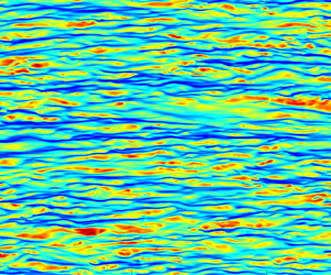
To characterize vividly the relationship between the velocity and the temperature structures, figure 3 shows the top view of the instantaneous  $u_d^{''+}$ and $T^{'+}$ fields of the case Ma15Re20K at three selected wall-normal positions. Other cases share similar characteristics and are not shown here for brevity. For the near-wall position $y^*\approx 10$, where $R_{u_d^{\prime \prime } T^{\prime }}\approx 1$, the velocity and temperature streaks share virtually identical morphological characteristics and the occurrences of the corresponding extreme events are roughly synchronous. For the logarithmic region $y\approx 0.15h$ with $R_{u_d^{\prime \prime } T^{\prime }}\approx 0.67$, the length scales of the velocity streaks become larger, whereas the temperature fluctuations display the mushroom shapes and are more isotropic than their near-wall counterparts. However, it is still effortless to observe the strong links between the low-speed velocity streaks and the negative temperature fluctuations. When the observation wall-normal position is moved to the channel centre $y\approx 0.85h$ with $R_{u_d^{\prime \prime } T^{\prime }}\approx 0.26$, in contrast to the velocity fluctuations shown in figure 3(e), the temperature fluctuations are characterized by spotted extreme events without discernible streaky shapes. The shapes of $T'$ structures are more isotropic. It underscores the fact that the coupling between the two fields is rather weak in the outer region. The above inspections, which are conducted at various wall-normal planes, are consistent with the variation tendency of $R_{u_d^{\prime \prime } T^{\prime }}$ as seen in figure 2(c). It is interesting to note that Pirozzoli & Bernardini (Reference Pirozzoli and Bernardini2011) also reported comparable findings on the temperature streaks for a supersonic boundary layer with adiabatic wall condition at a similar $Re_{\tau }$.
(a,c,e) Top view of the instantaneous density-weighted streamwise velocity fluctuation field  $u_d^{''+}$ at (a) $y^*\approx 10$, (c) $y\approx 0.15h$ and (e) $y\approx 0.85h$ for the case Ma15Re20K; (b,d,f) top view of the instantaneous temperature fluctuation field $T^{'+}$ at (b) $y^*\approx 10$, (d) $y\approx 0.15h$ and (f) $y\approx 0.85h$ for the case Ma15Re20K.

Finally, it is instructive to compare the premultiplied spectra of  $u_d''$ and $T'$ at different wall-normal positions (denoted as $kE_{\psi \psi }$, where $\psi$ can be $u_d''$ or $T'$), which are exhibited in figure 4. The specific spectral peak at a given wall-normal position may not be identical for each case, considering their distinct Reynolds numbers. We only show the results of the case Ma15Re20K here due to its relatively sufficient scale separation. To facilitate comparison, these spectra are normalized by the energy of $\psi$ at a given wall-normal height. The premultiplied spectra of $u_d''$ and $T'$, whether the streamwise or the spanwise spectra, almost overlap with one another in the buffer layer. Moreover, their peaks are located at $\lambda _x^*\approx 1000$ and $\lambda _z^*\approx 100$, which are consistent with the well-documented spectral scale characteristics of the near-wall turbulence in incompressible flow (Kline et al. Reference Kline, Reynolds, Schraub and Runstadler1967; Kim, Moin & Moser Reference Kim, Moin and Moser1987; Hwang Reference Hwang2013). When the observation wall-normal location is moved to the logarithmic layer, their disparities start to stand out. It can be seen that the typical streamwise length scales of velocity streaks are longer than those of the temperature, but their spanwise length scales are nearly identical, i.e. $\lambda _z\approx 0.8h$, just like those in incompressible flows (Ahn et al. Reference Ahn, Lee, Lee, Kang and Sung2015; Abe, Antonia & Toh Reference Abe, Antonia and Toh2018). In the outer region, the peaks of their streamwise spectra are still divergent, that is, $\lambda _x\approx 2h$ and $\lambda _x\approx 1h$ for $u_d''$ and $T'$, respectively. However, their spectral peaks of the spanwise spectra share equivalent length scale $\lambda _z\approx 1.4h$. Hence, the shapes of the temperature streaks are more isotropic than those of velocity streaks in the outer region. Overall, the spanwise length scales of $T'$ are in line with those of $u_d''$ spanning the whole channel. As the attached eddies are self-similar with their spanwise length scales (Lozano-Durán et al. Reference Lozano-Durán, Flores and Jiménez2012; Hwang Reference Hwang2015; Cheng et al. Reference Cheng, Li, Lozano-Durán and Liu2019), it underlines the fact again that the temperature fluctuation in compressible flow can also be treated as an attached variable. It also signifies that the $H_w$, a wall-based kernel function introduced in § 2.2, is of physical significance. In the next section, we elaborate on dissecting the coupling between $u_d''$ and $T'$ within the linear-model framework built in § 2.2. Furthermore, the statistical characteristics of $T'$ will also be investigated through the prism of the AEM.
(a,c,e) Premultiplied streamwise spectra of  $u_d''$ and $T'$ at (a) $y^*\approx 10$, (c) $y\approx 0.15h$ and (e) $y\approx 0.85h$ for the case Ma15Re20K; (b,d,f) premultiplied spanwise spectra of $u_d''$ and $T'$ at (b) $y^*\approx 10$, (d) $y\approx 0.15h$ and (f) $y\approx 0.85h$ for the case Ma15Re20K. These spectra are normalized by the energy of $\psi$ at a given wall-normal height.

4. Results of linear-model-based analysis
The linear-model-based analysis includes two branches, i.e.  $y_m=y_p$ and $y_m \neq y_p$ for (2.1) to (2.3). The former represents that the wall-normal position of the inputted $u_d''$ is the same as that of $T'$, whereas the latter is the opposite. The results of them will be reported in turn.
4.1. Linear-model-based analysis with $y_m=y_p$

4.1.1. Overall picture
Before proceeding with the detailed analysis, it is better to have a rough idea of the effectiveness of the linear coupling model. The dashed lines in figure 2(a,b) show the magnitudes of  $\overline {T_p^{'2}}^{+}$ as functions of $y_p/h$ and $y_p^*$ for all the supersonic cases, respectively. Here, $T_p'$ is calculated by an $H_T-$based estimation according to (2.1) and (2.2). It can be seen that only below the buffer layer can the temperature fluctuation intensities be largely captured by the linear model. This observation can be further verified by inspecting the relative deviations (RDs) displayed in figure 5. The definition of RD takes the form of
 \begin{equation} \mathrm{RD}=\frac{\overline{T^{'2}}^{+}-\overline{T_p^{'2}}^{+}}{\overline{T^{'2}}^{+}}. \end{equation}
The linear model can recover over  $95\,\%$ of $\overline {T^{'2}}^{+}$ for $y_p^*<10$. This relative error, however, rapidly increases as the wall-normal height increases. Taking the case Ma15Re20K as an example, only $50\,\%$ fluctuation intensity of $T'$ can be adequately captured at $y_p^*\approx 100$. An interesting thing worthy of note is that, for the case with the highest Reynolds number, there is a wall-normal position in the outer region, $y_p\approx 0.5h$, where RD begins to increase more rapidly than in the logarithmic region. This indicates that the effectiveness of the linear coupling model degenerates more severely as $y_p$ approaches the channel centre. The overall variation tendency is consistent with the correlations shown in figure 2(c), and it is reminiscent of the variation of the similarity between the velocity and temperature fluctuations in incompressible flow at the molecular Prandtl number $Pr$ close to unity. That is, there is a strong similarity in the near-wall region, while it is weakened away from the wall (Abe & Antonia Reference Abe and Antonia2009; Antonia et al. Reference Antonia, Abe and Kawamura2009; Pirozzoli, Bernardini & Orlandi Reference Pirozzoli, Bernardini and Orlandi2016). However, based on the linear model, the temperature fluctuation intensity $\overline {T^{'2}}^{+}$ can be decomposed as
 \begin{equation} \overline{T^{'2}}^{+}=\overline{T_p^{'2}}^{+}+\overline{T_{np}^{'2}}^{+}+2\overline{T_p'T_{np}'}^{+}. \end{equation}
Figure 5(c) shows the variations of  $\overline {T^{'2}}^{+}$, $\overline {T_p^{'2}}^{+}$, $\overline {T_{np}^{'2}}^{+}$ and $\overline {T_p'T_{np}'}^{+}$ as functions of the wall-normal height $y_p^*$ for the case Ma15Re20K. As seen, the magnitudes of $\overline {T_p^{'2}}^{+}$, $\overline {T_{np}^{'2}}^{+}$ are non-negligible, whereas $\overline {T_p'T_{np}'}^{+}$ nearly equals zero. It indicates that the interaction between $T_p'$ and $T_{np}'$ have no contribution to the even-order moments of $T'$. Other cases show similar results. We will ignore this interaction term in the following study.
(a,b) Relative deviations (RDs) as functions of (a)  $y_p/h$ and (b) $y_p^*$ for all the supersonic cases. Here, $y_p$ is equal to $y_m$ for these cases under consideration; (c) variations of $\overline {T^{'2}}^{+}$, $\overline {T_p^{'2}}^{+}$, $\overline {T_{np}^{'2}}^{+}$ and $\overline {T_p'T_{np}'}^{+}$ as functions of the wall-normal height $y_p^*$ for the case Ma15Re20K.

Accordingly, the entire channel can be divided into three regions for the purpose of the linear-model-based analysis: (1) the near-wall region, where RD $\,\approx\, 5\,\%$; (2) the logarithmic region and the lower part of the outer region; and (3) the outer region in the vicinity of the channel centre, where the effectiveness of the linear coupling model is the worst. We will dissect these three regions separately and shed light on the linear coupling relationship between $u_d''$ and $T'$ in the following subsections.
4.1.2. Near-wall region ($y_m^*=y_p^*\approx 10$)

We recall from (2.3) that  $\gamma ^{2}_{c}$ is a measure of coherence between $T'(y_p)$ and $u_d''(y_m)$ ( $\gamma ^{2}_{c}=1$ indicates a prefect coherence and $\gamma ^{2}_{c}=0$ indicates no coherence). Figure 6(a) shows the $\gamma ^{2}_{c}$ spectrum when $y_m^*=y_p^*\approx 10$ for the case Ma15Re20K. It is interesting to note that the temperature streaks are perfectly coherent with the velocity streaks at the typical near-wall turbulence length scales ( $\lambda _x^*\approx 1000$ and $\lambda _z^*\approx 100$, see figure 4a,b). It shows that the streamwise velocity fluctuations and temperature fluctuations carried by the near-wall motions are entirely coherent. This is the reason why $R_{u_d^{\prime \prime } T^{\prime }}\approx 1$ in the buffer layer (see figure 2c). Moreover, we note that for the large-scale temperature fluctuations ( $\lambda _x>1h$ and $\lambda _z>0.5h$), the magnitudes of $\gamma ^{2}_{c}$ also approach unity. It implies that the footprints of large-scale $T'$ and $u_d''$ in the near-wall region are also well coherent. In contrast, only the small-scale and ‘fat’ motions ( $\lambda _z^*>\lambda _x^*$) lose the perfect coherence. Other cases bear similar results and are not shown here for brevity.
(a) The  $\gamma ^{2}_{c}$ spectrum for the case Ma15Re20K when $y_m^*=y_p^*\approx 10$; (b) $R_{pm}$ spectrum for the case Ma15Re20K when $y_m^*=y_p^*\approx 10$. The dashed lines in panels (a,b) denote $\lambda _x^*=\lambda _z^*$.

Another way to gauge the linear coupling between these two signals is to investigate the relative magnitude  $R_{pm}$ associated with $\hat {T}_p'$ and $\hat {T}'$ at different length scales (Gupta et al. Reference Gupta, Madhusudanan, Wan, Illingworth and Juniper2021), namely,
 \begin{equation} R_{pm}(\lambda_{x},\lambda_{z}; y_m, y_p)=\sqrt{\langle|\hat{T}_p'(\lambda_{x},\lambda_{z}; y_m, y_p)|^2\rangle/\langle|\hat{T}'(\lambda_{x},\lambda_{z}; y_p)|^2\rangle}, \end{equation}
which are shown in figure 6(b) for the case M15Re20K. It appears that the energy of the streamwise elongated structures ( $\lambda _x^*>\lambda _z^*$) can be almost completely recovered by the linear model, whereas for those of the ‘fat’ motions ( $\lambda _z^*>\lambda _x^*$), the present approach loses some capabilities. This scenario is consistent with the $\gamma ^{2}_{c}$ spectrum shown in figure 6(a). We have checked that almost all the morphological properties of the instantaneous $T^{'+}$ displayed in figure 3(b) are recovered by $T_p^{'+}$ (not shown here). This is because the majority of the energetic motions populating the buffer layer are captured by the linear model.
At the end of this subsection, it is instructive to compare the probability density functions (p.d.f.s) of  $T_p^{'+}$ and $T^{'+}$ to distinguish whether some extreme events of $T^{'+}$ are predictable for the linear model. They are plotted in figure 7(a–c). For the positive extreme events ( $T^{'+}>0$), the linear model overestimates their probabilities of occurrence, whereas for the negative extreme events ( $T^{'+}<0$), the contrary is the case. The Reynolds number has no bearing on the conclusion. In other words, even while the linear coupling model can recapture the fundamental properties of the temperature field in the buffer layer, it is not able to reliably identify the extreme thermal events. Figure 7(d) shows the p.d.f.s of $T_p'(y_p^*=y_m^*\approx 10)$, $T'(y^*\approx 10)$ and $u_d''(y^*\approx 10)$ for the case Ma15Re20K. To facilitate comparison, each variable is normalized by its r.m.s. value. Other cases show similar results and are not shown here. A noteworthy observation is that the p.d.f. of $T_p'$ bears similar shape with that of $u_d''$ rather than $T'$. This is the limitation of the linear model, i.e. the instantaneous distribution of the predicted variable is controlled by that of the measured variable (the results of other wall-normal positions also obey this criterion, see figures 11c and 18b). Only with quadratic estimation techniques and above can the p.d.f. of the predicted variable be modified and closer to the actual flow (Tinney et al. Reference Tinney, Coiffet, Delville, Hall, Jordan and Glauser2006).
(a,b,c) The p.d.f.s of  $T_p^{'+}(y_p^*=y_m^*\approx 10)$ and $T^{'+}(y^*\approx 10)$ for the case (a) Ma15Re3K, (b) Ma15Re9K and (c) Ma15Re20K. (d) The p.d.f.s of $T_p'(y_p^*=y_m^*\approx 10)$, $T'(y^*\approx 10)$ and $u_d''(y^*\approx 10)$ for the case Ma15Re20K. Each variable is normalized by its root mean square (r.m.s.) value in panel (d). The $\psi$ in the abscissa of panel (d) stands for the corresponding variable.

4.1.3. Logarithmic region ($y_m=y_p\approx 0.1h\unicode{x2013}0.2h$)

For the logarithmic region, the effectiveness of the linear model is not as excellent as it is in the buffer layer. Taking the case Ma15Re20K as an example, at  $y_m=y_p\approx 0.15h$, the RD is $55\,\%$. A non-negligible fraction of fluctuation intensity cannot be captured by the linear model.
The  $\gamma ^{2}_{c}$ spectra of the case Ma15Re20K for $y_m=y_p\approx 0.1h$, $0.15h$ and $0.2h$ are shown in figures 8(a), 8(c) and 8(e), respectively. It is noted that we only report the results of case Ma15Re20K in this subsection due to its relatively wider spanning of the logarithmic region. It is not difficult to observe that only the streamwise elongated fluctuations ( $\lambda _x>\lambda _z$) of $T'$ and $u_d''$ are highly coupled. This scenario is identical to that of the buffer layer (see figure 6). Additionally, there is only a small portion of the scale range where the magnitude of $\gamma ^{2}_{c}$ is remarkable. By dissecting the $\gamma ^{2}_{c}$ spectra of the disparate wall-normal positions in the logarithmic region displayed in figure 8, this range can be roughly bounded by
 \begin{equation} \lambda_x>\lambda_z,\quad \lambda_x>10y_p,\quad \lambda_z>2y_p. \end{equation}
Figure 8(b,d,f) show the  $R_{pm}$ spectra at the corresponding three wall-normal locations, respectively. It is transparent that the energy in the range defined by (4.4a–c) can be predominantly recovered by the linear model. The scale-based linear coupling can also be recognized by comparing the instantaneous $T^{'+}$ and $T_p^{'+}$ at $y=0.15h$, which are illustrated in figure 9(a). As seen, only the long streaks of $T^{'+}$ are maintained in the instantaneous $T_p^{'+}$. Additionally, $T_p^{'+}$ resembles the filtered $u_d^{''+}$ (see figure 3c), and $T_p^{'+}$ and $T^{'+}$ (see figure 3d) seem to organize similarly along the spanwise direction rather than the streamwise direction. These observations are similar to the finite similarities between the velocity and scalar fields reported in incompressible wall turbulence (Antonia et al. Reference Antonia, Abe and Kawamura2009).
(a,c,e) The  $\gamma ^{2}_{c}$ spectra for the case Ma15Re20K when (a) $y_m=y_p\approx 0.1h$, (c) $y_m=y_p\approx 0.15h$, (e) $y_m=y_p\approx 0.2h$; (b,d,f) $R_{pm}$ spectra for the case Ma15Re20K when (b) $y_m=y_p\approx 0.1h$, (d) $y_m=y_p\approx 0.15h$, (f) $y_m=y_p\approx 0.2h$. The dashed oblique lines in panels (a,c,e) denote $\lambda _x=\lambda _z$, and the dashed transverse and the vertical lines denote $\lambda _z=2y_p$ and $\lambda _x=10y_p$, respectively.

(a) Top view of the instantaneous  $T_p^{'+}$ field when $y_m=y_p\approx 0.15h$ for the case Ma15Re20K. (b) Variation of $\lambda _z^{\star }/h$ as a function of $y_p/h$ in the logarithmic region for Ma15Re20K. In panel (b), the DNS results are presented by circles and the black line denotes $\lambda _z^{\star }=3.6y_p$.

Moreover, some details also deserve attention. First, the peaks of  $\gamma ^{2}_{c}$ are located at $\lambda _z\approx 1h\unicode{x2013}1.5h$ for the three selected wall-normal positions, which is the spanwise spacing of the very-large-scale motions (VLSMs) in the outer region of the incompressible and supersonic turbulent boundary layers (Del Álamo & Jiménez Reference Del Álamo and Jiménez2003; Abe et al. Reference Abe, Kawamura and Choi2004a; Ganapathisubramani, Clemens & Dolling Reference Ganapathisubramani, Clemens and Dolling2006; Hutchins & Marusic Reference Hutchins and Marusic2007). It signifies that VLSMs can not only permeate into the near-wall and the logarithmic regions, but also be actively linked with the temperature streaks in the compressible wall turbulence. Second, it is intriguing that the range boundaries defined by (4.4a–c) follow the scales of the self-similar wall-attached motions in wall turbulence. To name but a few, Deshpande, Monty & Marusic (Reference Deshpande, Monty and Marusic2021) analysed the scale characteristics of the active motions (i.e. the self-similar attached eddies) in the logarithmic region of the boundary layers, and found their geometric shapes obey $\lambda _x\approx 10y$ and $\lambda _z\approx 3y$. Hwang, Lee & Sung (Reference Hwang, Lee and Sung2020) also pointed out that the lower bound of the linear behaviours of the self-similar wall-attached structures in wall turbulence follows $\lambda _x>12y$ and $\lambda _x=4\lambda _z$. These pioneer results are all very close to the scale-range estimation provided by (4.4a–c). Hence, it is sensible to envision that the temperature streaks coupling the velocity field in the compressible flow are considerably wall-attached. They consist of two components, e.g. one is the self-similar wall-attached motions described by the AEM (Townsend Reference Townsend1976; Perry & Chong Reference Perry and Chong1982); the other is VLSMs which can also exert significant influences on the near-wall flow (Perry & Marusic Reference Perry and Marusic1995; Cheng et al. Reference Cheng, Li, Lozano-Durán and Liu2019; Yoon et al. Reference Yoon, Hwang, Yang and Sung2020).
To further characterize the energetic scales in LCS of the logarithmic region, we define the  $\gamma _c^2-$weighted average spanwise wavenumber $k_z^{\star }(y)$ and the corresponding length scale $\lambda _z^{\star }=2{\rm \pi} /k_z^{\star }(y)$. The definition of $k_z^{\star }$ takes the form of
 \begin{equation} k_z^{{\star}}(y)=\frac{\displaystyle\int_{\varOmega} k_z \gamma_c^2(y ; k_x, k_z)\, \mathrm{d} k_x \,\mathrm{d} k_z}{\displaystyle\int_{\varOmega} \gamma_c^2(y ; k_x, k_z)\, \mathrm{d} k_x \,\mathrm{d} k_z}, \end{equation}
where  $\varOmega$ is the spectral domain defined by (4.4a–c), i.e. the energetic scale range of the LCS in the logarithmic region. It is the spanwise length scale rather than the streamwise one that is taken into account here, as previous studies provide compelling evidence that the energy-containing motions in the logarithmic region are self-similar with their spanwise length scales (Del Álamo et al. Reference Del Álamo, Jiménez, Zandonade and Moser2004; Hwang Reference Hwang2015; Cheng et al. Reference Cheng, Li, Lozano-Durán and Liu2019). Figure 9(b) shows the variation of $\lambda _z^{\star }/h$ as a function of $y_p/h$ in the logarithmic region for Ma15Re20K. It can be seen that there is a linear relationship between $\lambda _z^{\star }/h$ and $y_p/h$. This observation underscores the fact that the temperature and velocity fields are linearly coupled within the self-similar scale range. The variation of $\gamma _c^2$ spectra along the wall-normal direction in the logarithmic region is chiefly ascribed to the self-similar eddies.
The above argument can also be validated by inspecting the  $\gamma ^{2}_{w}$ spectra of $T_p^{'+}$ and $T_{np}^{'+}$ as per (2.8), which evaluate the wall coherence of these two signals. Herein, $T_{np}'=T'-T_p'$ is the uncoupling component of $T'$. The results are displayed in figure 10 for the three corresponding wall-normal planes in the logarithmic region. Only the motions of $T_p'$ within the scale range roughly given by (4.4a–c) are coherent with the near-wall flow, whereas for $T_{np}'$, no coherence can be observed. This observation supports our claim above. Nearly all the wall-attached temperature streaks are contained in $T_p'$, rather than $T_{np}'$. It is noted that the $\gamma ^{2}_{w}$ spectra given here (figure 10a,c,e) and the $\gamma ^{2}_{c}$ spectra shown in figures 8(a), 8(c) and 8(e) are not identical. It suggests that some $T'$ motions coupled with $u_d''$ are wall-detached in the logarithmic region indeed.
(a,c,e) The  $\gamma ^{2}_{w}$ spectra of $T_p^{'+}$ for the case Ma15Re20K when (a) $y_m=y_p\approx 0.1h$, (c) $y_m=y_p\approx 0.15h$ and (e) $y_m=y_p\approx 0.2h$; (b,d,f) $\gamma ^{2}_{w}$ spectra of $T_{np}^{'+}$ for the case Ma15Re20K when (b) $y_m=y_p\approx 0.1h$, (d) $y_m=y_p\approx 0.15h$ and (f) $y_m=y_p\approx 0.2h$. The dashed oblique lines in the panels denote $\lambda _x=\lambda _z$, and the dashed transverse and the vertical lines denote $\lambda _z=2y_p$ and $\lambda _x=10y_p$, respectively.

Figure 11(a) shows the variations of the fluctuation intensities of  $T'$,
$T'$,  $T_p'$, $T_{p,w}'$ and $T_{np,w}'$ as functions of the wall-normal height $y/h$ in the logarithmic region. Herein, $T_{p,w}'$ and $T_{np,w}'$ are the wall-attached components of $T_{p}'$ and $T_{np}'$, respectively, which can be estimated by an $H_w$-based estimation according to (2.6) and (2.7). As can be seen, the intensity of $T_{p,w}'$ occupies approximately $34\,\%$ of $\overline {T_{p}^{'2}}^{+}$ in the logarithmic region (equivalent to $15\,\%$ of $\overline {T^{'2}}^{+}$), whereas the magnitude of $T_{np,w}'$ is negligible. It shows once again that almost all the temperature streaks that are attached to the wall are contained in $T_p'$ rather than $T_{np}'$. Figure 11(b) compares the p.d.f.s of the instantaneous $T^{'}$, $T_p^{'+}$ and $T_{p,w}^{'+}$ at $y/h=0.1$. The p.d.f. of $T_{p,w}^{'+}$ is found to be more symmetric than those of the other two signals with invisible extreme events. This phenomenon hints that the small-scale $T'$ motions, which cannot be captured by the linear model, are more intermittent than the large-scale counterparts. Figure 11(c) displays the p.d.f.s of $T'$,
$T'$,  $T_p'$ and $u_{d}''$ at $y/h=0.1$. All variables are normalized by their r.m.s. values. As expected, the p.d.f. of $T_p'$ has a similar shape with that of $u_d''$.
(a) Variations of the fluctuation intensities of  $T'$,
$T'$,  $T_p'$, $T_{p,w}'$ and $T_{np,w}'$ as functions of the wall-normal height $y/h$ in the logarithmic region for the case Ma15Re20K; (b) p.d.f.s of the instantaneous $T^{'+}$, $T_p^{'+}$ and $T_{p,w}^{'+}$ at $y/h=0.1$ for the case Ma15Re20K; (c) p.d.f.s of the instantaneous $T^{'}$, $T_p'$ and $u_{d}''$ at $y/h=0.1$ for the case Ma15Re20K. Each variable is normalized by its r.m.s. value in panel (c). The $\psi$ in the abscissa of panel (c) stands for the corresponding variable.

Since it is demonstrated that the wall-attached component of  $T'$ is contained in $T_p'$, it is instructive to inspect its statistical characteristics and compare with the celebrated attached-eddy hypothesis (Townsend Reference Townsend1976; Perry & Chong Reference Perry and Chong1982). In our previous work (Cheng & Fu Reference Cheng and Fu2022a), we have proposed an operable framework to reach this goal. To be specific, for a wall-attached variable $\phi$ in the logarithmic region between $y_s^*$ and $y_p^*$ ( $y_s^*$ denotes the lower bound of the logarithmic region and is set as 80 in the present study), if its representative spatial structures are arranged in a hierarchical manner which can be adequately depicted by the AEM, the momentum generation function of its footprint in the near-wall region ( $\phi _L$) should follow a so-called strong self-similarity (SSS), i.e.
 \begin{equation} \langle \exp(q\phi_L)\rangle\sim \left(\frac{y_p}{y_s}\right)^{s(q)}, \end{equation}
where  $\langle \exp (q\phi _L)\rangle$ is the momentum generation function, $q$ is a real number, which can be chosen optionally, $s(q)=C_1\ln \langle \exp (qa)\rangle$ is called anomalous exponent, $C_1$ is a constant and $a$ is a random additive, which represents the footprint of $\phi$ in the near-wall region generated by the attached eddies at a given wall-normal height. The parameter $q$ in the momentum generation function serves as a ‘controller’ to highlight different components of $\phi _L$ (Yang, Marusic & Meneveau Reference Yang, Marusic and Meneveau2016). To be specific, a positive $q$ emphasizes the positive component of $\phi _L$ and vice versa. Furthermore, the $n$th-order moment of $\phi _L$ can be derived by (Yang et al. Reference Yang, Marusic and Meneveau2016)
 \begin{equation} \langle \phi_L^n\rangle= \left.\frac{\partial^{n} \langle \exp(q\phi_L)\rangle}{\partial q^{n}}\right|_{q=0}. \end{equation}
This relationship will be employed in § 5.1.
If  $a$ is a Gaussian variable, the anomalous exponent can be recast as
 \begin{equation} s(q)=C_2q^2, \end{equation}
where  $C_2$ is another constant. However, an extended self-similarity (ESS) is defined to describe the relationship between $\langle \exp (q\phi _L)\rangle$ and $\langle \exp (q_0\phi _L)\rangle$ (fixed $q_0$) (Benzi et al. Reference Benzi, Ciliberto, Tripiccione, Baudet, Massaioli and Succi1993), i.e.
 \begin{equation} \langle \exp(q\phi_L)\rangle = \langle \exp(q_0\phi_L)\rangle^{\xi(q,q_0)}, \end{equation}
where  $\xi (q,q_0)$ is a function of $q$ (fixed $q_0$). Note that the validity of ESS depends on the hierarchical structures of $\phi$ in the logarithmic region, dominantly. A more detailed derivation of the SSS and the ESS associated with the footprints of the attached eddies can be found in Cheng & Fu (Reference Cheng and Fu2022a).
For the footprints of the temperature fluctuations in supersonic channel flows, they can be obtained by following (2.4) and (2.5) with  $T_{\psi }'=T_p'$. Concurrently, we can further define a moment generation function based on this estimation. It takes the form of
 \begin{equation} G(q,y_p)=\langle \exp(q(T_{p,L}^{'+}(y_s,y_i)-T_{p,L}^{'+}(y_p,y_i)))\rangle, \end{equation}
where  $T_{p,L}^{'+}(y_s,y_i)-T_{p,L}^{'+}(y_p,y_i)$ is the footprint of $T_{p}^{'+}$ generated by the attached eddies with their wall-normal heights varying from $y_s$ to $y_p$, which resembles the $\phi _L$ in (4.6) and (4.9). Here, $T_{p,L}'$ is calculated by an $H_L-$based estimation according to (2.4) and (2.5). As per the hierarchical attached eddies in high-Reynolds-number wall turbulence, $T_{p,L}^{'+}(y_s,y_i)$ is the superposition at $y_i$ contributed from the wall-coherent motions with their heights larger than $y_s$. Thus, the difference value $T_{p,L}^{'+}(y_s,y_i)-T_{p,L}^{'+}(y_p,y_i)$ can be interpreted as the superposition contribution generated by the wall-coherent eddies with their wall-normal heights within $y_s$ to $y_p$ (Cheng & Fu Reference Cheng and Fu2022a; Cheng et al. Reference Cheng, Shyy and Fu2022). The above process is not applied to $T_{np}^{'+}$, because we have verified that $T_{np}^{'+}$ is not coherent with the near-wall flow and does not bear a footprint (see figures 10 and 11a).
Figure 12(a) shows the variations of  $G$ as a function of $y_p/y_s$ for $q=\pm 5$ and $q=\pm 3$. Power-law behaviours can be found in the interval $1.1\le y_p/y_s\le 1.8$ for both positive and negative $q$, justifying the validity of SSS, i.e. (4.6). This observation highlights that the superpositions of wall-attached $T'$ on the wall surface follow an additive process. Additionally, the positive and negative components of $T_{p,L}^{'+}(y_s,y_i)-T_{p,L}^{'+}(y_p,y_i)$ are comparatively symmetrical (for lower Mach number, the asymmetries are more obvious, see § 5.1). Furthermore, in an incompressible channel flow, the asymmetries between the footprints of the high-speed and the low-speed $u'$ motions are quite evident, see Cheng & Fu (Reference Cheng and Fu2022a). Other $q$ values yield similar results and are not shown here for brevity. The anomalous exponent $s(q)$ can be obtained by fitting the range $1.1\le y_p/y_s\le 1.8$, where both positive and negative $q$ display good power-law scalings. Figure 12(b) shows the variation of the anomalous exponent $s(q)$ as a function of $q$. The solid line denotes the quadratic fit within $-1\le q \le 1$. It can be seen that the variation of $s(q)$ still follows a quadratic law at large $| q |$. Moreover, the skewness and flatness of the footprints of $T'$ generated by the attached eddies across the whole logarithmic region are $-$0.22 and 3.11 (the counterparts of $u'$ in an incompressible turbulent channel flow at $Re_{\tau }=2003$ are 0.05 and 2.91 (Cheng & Fu Reference Cheng and Fu2022a)). These observations signify that the near-wall heat flux generated by the attached eddies at a given wall-normal height can also be simply treated as a Gaussian variable for modelling purposes (though a little super-Gaussian) at this $M_b$. In the next section, we will discuss the Mach number effects on these statistics.
(a) The variations of  $G$ as a function of $y_p/y_s$ for $q=\pm 5$ and $q=\pm 3$; (b) anomalous exponent $s(q)$ as a function of $q$. The line in panel (b) is a quadratic fit. The data are taken from the case Ma15Re20K.

Different from SSS, ESS only relies on the hierarchical structures of  $T'$ in the logarithmic region. Figure 13(a,b) shows the ESS scalings for $q_0=-2$ and $q_0=2$, respectively. As seen, ESS holds for the entire logarithmic region. This observation suggests that the generation of the near-wall heat flux by the multi-scale logarithmic motions obeys an additive process.
The variations of (a)  $G(q)$ as functions of $G(-2)$ for $q=-1,-3,-5$; (b) $G(q)$ as functions of $G(2)$ for $q=1,3,5$. Both vertical and horizontal axes in panels (a) and (b) are plotted in logarithmic form. The data are taken from the case Ma15Re20K.

In summary, in the logarithmic region, the  $T'$ motions are found to be linearly coupled with the streamwise velocity fluctuations at the scales which are corresponding to the attached eddies and the VLSMs. The wall-attached structures contribute nearly $34\,\%$ of $\overline {T_{p}^{'2}}^{+}$ in the logarithmic region (equal to $15\,\%$ of $\overline {T^{'2}}^{+}$). By dissecting their footprints, it is demonstrated that $T'$ motions in the logarithmic region are organized as hierarchical structures and can be described by the AEM. This observation is consistent with some recent studies on the temperature field in compressible wall turbulence (Cheng & Fu Reference Cheng and Fu2022b; Yu et al. Reference Yu, Xu, Chen, Liu, Fu and Yuan2022; Yuan et al. Reference Yuan, Tong, Li, Chen and Dong2022). Moreover, we further reveal that their footprints are non-intermittent and Gaussian in a supersonic channel flow.
4.1.4. Outer region ($y_m=y_p\approx 0.85h$)

As  $y_m$( $y_p$) moves into the outer region, the linear coupling between $u_d''$ and $T'$ becomes weaker. This phenomenon is more obvious at the outer region near the channel centre. This is to be anticipated since $u_d''$ and $T'$ are only linearly coupled at larger scales as $y_m$( $y_p$) increases, as per our study above. In this subsection, we further shed light on this fact. We only show the results of the case Ma15Re20K due to its relatively higher Reynolds number.
Figure 14(a,b) illustrate the  $\gamma ^{2}_{c}$ and $R_{pm}$ spectra for $y_m=y_p\approx 0.85h$, respectively. Intriguingly, the two spectra are only non-trivial at $\lambda _z>1h$ and $\lambda _x>2h$, which are significantly different from those in the logarithmic and the near-wall regions. Only VLSMs of $T'$ and $u_d^{\prime \prime }$ are weakly coupled. Another interesting observation which deserves attention is that these coupled motions are not isotropic as the scale characteristics of $T^{'+}$ in the outer region (see figure 4f). In contrast, they resemble the scale characteristics of $u_d^{''+}$ in the outer region (see figure 4e). In other words, $T_p^{'+}$ is ‘passive’ in shaping their scale properties. Figure 15(a,b) display the instantaneous $T^{'+}$ and $T_p^{'+}$ for $y_m=y_p\approx 0.85h$, respectively. Apparently, the motions of $T_p^{'+}$ emerge like those of $u_d^{\prime \prime +}$ (figure 3e) rather than $T^{'+}$.
(a) The  $\gamma ^{2}_{c}$ spectrum when $y_m=y_p\approx 0.85h$ for the case Ma15Re20K; (b) $R_{pm}$ spectrum when $y_m=y_p\approx 0.85h$ for the case Ma15Re20K.

(a) Top view of the instantaneous  $T^{'+}$ field when $y_m=y_p\approx 0.85h$; (b) top view of the instantaneous $T_p^{'+}$ field when $y_m=y_p\approx 0.85h$. The data are taken from the case Ma15Re20K.

All in all, for the first branch of the linear-model-based analysis, i.e.  $y_p=y_m$, the applicability of SLSE depends on the wall-normal location in the boundary layer and is closely related to the energy-containing motions residing in it. In the next section, we are dedicated to another branch, namely $y_p\neq y_m$.
4.2. Linear-model-based analysis with $y_m\neq y_p$

For this branch of the linear-model-based analysis, we only consider one realization, i.e.  $y_m>y_p$ with $y_m$ being in the logarithmic region. That is to say, what we pursue here is the estimation of the $T'$ in the near-wall region by invoking the $u_d''$ in the logarithmic region through the linear model. This study bears some practical significance. For example, it may be a guideline for the reconstruction of the temperature signals in the near-wall region by employing limited velocity signals recorded by a hot-wired probe in the logarithmic region. Hereafter, we adopt the case Ma15Re20K, and fix $y_m^*$ as $80$,
$80$,  $0.2h^*$ and $3.9\sqrt {Re_{\tau }^*}$ (namely the centre of the logarithmic layer (Mathis, Hutchins & Marusic Reference Mathis, Hutchins and Marusic2011), $y_m\approx 0.14h$ for Ma15Re20K). Concurrently, $y_p$ varies from the viscous sublayer to $y_m$. The reason we only use the case Ma15Re20K is due to its relatively higher Reynolds number than other cases.
Figure 16(a) shows the profiles of  $\overline {T_p^{'2}}^{+}$ within the range $0< y_p^*< y_m^*$ and the profile of $\overline {T^{'2}}^{+}$ is also included for comparison. Only a fraction of temperature fluctuations can be recovered by the linear model with inputs $u_d''$ from the logarithmic region. It is noted that the wall-normal location of the peaks of $\overline {T_p^{'2}}^{+}$ is identical to that of $\overline {T^{'2}}^{+}$ regardless of the locus of $y_m^*$, namely $y_p^*\approx 10$. This is under expectation, since the temperature fluctuations have more energy at this wall-normal position indeed. Figure 16(b) illustrates the variations of RD as functions of $y_p^*$. Only $10\,\%$ of $\overline {T^{'2}}^{+}$ can be captured by the linear model in the viscous sublayer. This ratio increases monotonously when $y_p$ approaches $y_m$.
(a) Profiles of  $\overline {T_p^{'2}}^{+}$ within the range $0< y_p^*< y_m^*$, and the profile of $\overline {T^{'2}}^{+}$ is also included for comparison; (b) variations of RD as functions of $y_p^*$. The data are taken from the case Ma15Re20K, and $y_m^* \approx 80$, $3.9\sqrt {Re_{\tau }^*}$ and $0.2h^*$.

Figure 17(a,b) shows the  $\gamma ^{2}_{c}$ and $R_{pm}$ spectra at $y_p^*\approx 10$ with $y_m^* \approx 3.9\sqrt {Re_{\tau }^*}$, respectively. The streamwise and spanwise length scales in the two figures are scaled in the outer unit rather than viscous unit, because the magnitudes of $\gamma ^{2}_{c}$ and $R_{pm}$ are observed to be non-negligible only at a large-scale range. Comparing with the $\gamma ^{2}_{w}$ spectrum of $T_p'$ displayed in figure 10(c) when $y_p=y_m\approx 0.15h$, it is not difficult to find that the $\gamma ^{2}_{c}$ spectrum here bears similar scale characteristics. It suggests that only the wall-attached superposition components contributed by the motions at $y_m$ are identified at $y_p$ by the linear model. Figure 17(b) also shows akin results.
(a) The  $\gamma ^{2}_{c}$ spectrum when $y_p^*=10$ for the case Ma15Re20K; (b) $R_{pm}$ spectrum when $y_p^*=10$ for the case Ma15Re20K. Here, $y_m^*$ is set as $3.9\sqrt {Re_{\tau }^*}$. The dashed oblique lines in the panels denote $\lambda _x=\lambda _z$, and the dashed transverse and the vertical lines denote $\lambda _z=2y_p$ and $\lambda _x=10y_p$, respectively.

Figure 18(a) further shows the p.d.f.s of  $T_p^{'+}(y_m\neq y_p)$ at $y_p^*\approx 10$ with $y_m^* \approx 3.9\sqrt {Re_{\tau }^*}$, and the counterparts of $T^{'+}(y^*=10)$ and $T_p^{'+}(y_m^*=y_p^*\approx 10)$ are also included for comparison. Comparing with the other two profiles, the p.d.f. of $T_p^{'+}(y_m\neq y_p)$ is rather symmetric with invisible extreme events. It signifies that in the near-wall region, only the long temperature streaks with mild fluctuation intensities have linkages with the motions in the logarithmic region. Furthermore, the near-wall flow should be given more consideration to control the extreme thermal events on the wall surface in supersonic wall turbulence, because, according to the results shown here, the intensities of the superposition components contributed by the motions populating the logarithmic and the outer regions are not that large indeed. Figure 18(b) displays the p.d.f.s of $T'(y^*\approx 10)$, $T_p'(y_m\neq y_p)$ at $y_p^*\approx 10$ and $u_{d}''(y_m)$ with $y_m^*\approx 3.9\sqrt {Re_{\tau }^*}$. Even though $y_m\neq y_p$, the p.d.f. shape of the predicted $T_p'$ at $y_p$ still conforms to that of $u_{d}''$ at $y_m$.
(a) The p.d.f.s of  $T_p^{'+}(y_m\neq y_p)$ at $y_p^*\approx 10$ with $y_m^*\approx 3.9\sqrt {Re_{\tau }^*}$, and the counterparts of $T^{'+}(y^*=10)$ and $T_p^{'+}(y_m^*=y_p^*\approx 10)$ are also included for comparison. (b) The p.d.f.s of $T_p'(y_m\neq y_p)$ at $y_p^*\approx 10$ with $y_m^*\approx 3.9\sqrt {Re_{\tau }^*}$, $T'(y^*=10)$ and $u_d''(y_m)$. Each variable is normalized by its r.m.s. value in panel (b). The $\psi$ in the abscissa of panel (b) stands for the corresponding variable. The data are taken from the case Ma15Re20K.

5. Discussion
5.1. Mach number effects
In this subsection, we are dedicated to shedding light on the Mach number effects on the linear coupling between  $u_d''$ and $T'$ by analysing the subsonic cases listed in table 1. We acknowledge that the DNS data with a higher Mach number (for example, $M_b=3.0$) are needed for conducting a more comprehensive study on this problem. However, the DNS of supersonic channel flows at both high Mach number and Reynolds number demands huge computational costs. A more extensive investigation of the Mach number effects will be carried out when the database is available.
Following the above manner, we start by taking the situation  $y_m=y_p$ into consideration. Figure 19(a,b) shows the variations of RD for all cases as functions of $y_p/h$ and $y_p^*$, respectively. The supersonic cases are illustrated by solid lines, whereas the subsonic ones by dashed lines. Apart from the two cases with $Re_{\tau }^*\approx 160$, the profiles of RD with similar $Re_{\tau }^*$ overlap with each other. The exceptions of the two cases may result from the low-Reynolds-number effects. It suggests that the Mach number has negligible effects on the linear coupling between $u_d''$ and $T'$. It is the Reynolds number $Re_{\tau }^*$ rather than Mach number that acts as a key similarity parameter in constructing their coupling. This observation is consistent with our previous work on the scale characteristics of the energy-containing motions in compressible channel flows (Cheng & Fu Reference Cheng and Fu2022b).
(a) Relative deviations (RDs) as functions of  $y_p/h$ for all the cases; (b) relative deviations (RDs) as functions of $y_p^*$ for all the cases. Here, $y_p$ equals to $y_m$ for these cases under consideration.

For  $y_p=y_m$ in the logarithmic region, all the wall-attached temperature streaks are found to be contained in $T_p'$ (not shown here), and the SSS (4.6) is examined and shown in figure 20 by analysing the case Ma08Re17K. Figure 20(a) shows the variations of $G$ as a function of $y_p/y_s$ for $q=\pm 5$ and $q=\pm 3$. It is particularly noteworthy that power-law behaviours can be found in the interval of $1.1\le y_p/y_s\le 1.6$ with discernible differences between $G(q)$ and $G(-q)$. By comparing with figure 12(a), it can be conjectured that the enlargement of the Mach number leads to the disappearance of the asymmetric characteristics between the positive and the negative footprints of $T'$ generated by the attached eddies.
(a) The variations of  $G$ as a function of $y_p/y_s$ with $q=\pm 5$ and $q=\pm 3$ for Ma08Re17K; (b) anomalous exponent $s(q)$ as a function of $q$ for Ma08Re17K. The solid line in panel (b) is a quadratic fit, and the dashed line is the result of the supersonic case Ma15Re20K, which is included here for comparison.

This assertion can also be validated by examining the variational tendency of the anomalous exponent  $s(q)$ (figure 20b). The profile of $s(q)$ of Ma08Re17K is not that symmetric with regards to $q$ and has an optimal $C_2\approx 0.00218$, in contrast to the result of Ma15Re20K (see figure 12b). It indicates that the distribution of near-wall heat flux generated by the attached eddies at a given wall-normal height deviates from the Gaussian distribution slightly at this Mach number. This scenario is altered by the increased compressibility of the supersonic flows. Moreover, it can also be noticed that the optimal $C_2$ of Ma08Re17K is remarkably different from that of Ma15Re20K (see blue dashed line in figure 20b). It strongly suggests that there is a striking difference in the Reynolds number dependence of the wall-heated flux fluctuation intensities at different $M_b$ for compressible channel flows. If we acknowledge that the Reynolds number dependence of wall heated flux fluctuation intensity can be ascribed to the superposition of the self-similar attached eddies (obviously, this is not true), the variational tendency of the temperature fluctuation intensity in the viscous sublayer contributed by the attached eddies can be predicted by (Yang et al. Reference Yang, Marusic and Meneveau2016; Cheng & Fu Reference Cheng and Fu2022a)
 \begin{equation} \left.\frac{\partial^{2} G(q,y_p)}{\partial q^{2}}\right|_{q=0} \sim 2C_2\ln(y_p/y_s). \end{equation}
Unequal  $C_2$ for subsonic and supersonic flows indicates their different variational tendencies with respect to $\ln (y_p/y_s)$. It underlines the fact that it is rather difficult to formulate the Reynolds number dependence of the wall heated flux at different Mach numbers by a unified formula without taking Mach number effects into account. For $y_p=y_m$ in the outer region close to the channel centre, the effectiveness of the linear model is limited. For sake of brevity, these results are not shown here.
At last, let us turn our attention to another situation with  $y_m \neq y_p$. Similarly, $y_m^*$ is fixed as $3.9\sqrt {Re_{\tau }^*}$ ( $y_m\approx 0.14h$ for Ma08Re17K), the centre of the logarithmic layer, and $y_p$ varies from the viscous sublayer to $y_m$. Figure 21 compares the variations of RD as a function of $y_p^*$ for Ma08Re17K and Ma15Re20K. For $y_p^*<50$, the RD of Ma15Re20K is larger than that of Ma08Re17K, whereas they overlap with each other for $y_p^*>50$. It may imply that the compressibility lessens the linkages between the near-wall temperature field and the energy-containing motions populating the logarithmic region slightly. The higher mean-temperature gradient of the supersonic case near the wall may preclude the permeation of the wall-attached eddies. Whether it holds or not at larger Mach number deserves further investigations.
Variations of RD as functions of  $y_p^*$ for the cases Ma08Re17K and Ma15Re20K. Here, $y_m^* \approx 3.9\sqrt {Re_{\tau }^*}$ (the vertical line) and $0< y_p^*< y_m^*$.

5.2. Strong Reynolds analogy: a heuristic study
By far, we have shown that the temperature and the velocity fluctuations are highly linked with each other through the prism of the multi-scale energy-containing eddies. However, the SRA (1.1), which is deduced from the momentum and the energy equations with some ideal hypotheses, indicates this interconnection from the mathematical statistics side (Morkovin Reference Morkovin1962). A question may be raised, e.g. can the present study be instructive to unravel the physical significance behind the SRA? In this subsection, we try to answer this question in a heuristic way.
Gaviglio (Reference Gaviglio1987) observed that, for a compressible boundary layer, the intensities of the velocity and the temperature fluctuations carried by large-scale eddies are in direct proportion to the gradients of their mean quantities. Additionally, their corresponding ratios are positively related to the velocity length scale ( $\ell _u$) and the temperature length scale ( $\ell _T$), respectively. In a statistical manner, this relationship can be expressed by
 \begin{equation} a \sqrt{\overline{T^{\prime 2}}} / \partial_y \bar{T}=\sqrt{\overline{u^{\prime 2}}} / \partial_y \bar{u}, \end{equation}
where  $a=\ell _u/\ell _T$, namely the ratio between the velocity and the temperature length scales. Equation (5.2) can be further cast as
 \begin{equation} \frac{\sqrt{\overline{T^{\prime 2}}} / \bar{T}}{(\gamma-1) M^2 \sqrt{\overline{u^{\prime 2}}} / \bar{u}}=\frac{1}{a(1-\partial \bar{T}_t / \partial \bar{T})}, \end{equation}
where  $\bar {T}_t$ denotes the mean total temperature. Gaviglio (Reference Gaviglio1987) and Rubesin (Reference Rubesin1990) modelled $a=1$ and $a=1.34$, which are denoted as GSRA and RSRA hereafter, respectively. Huang et al. (Reference Huang, Coleman and Bradshaw1995) further pointed out that $a$ should be strictly identical to the so-called turbulent Prandtl number $Pr_t$, whose definition takes the form of
 \begin{equation} Pr_t=\frac{\overline{\rho v^{\prime} u^{\prime}} \partial_y \bar{T}}{\overline{\rho v^{\prime} T^{\prime}} \partial_y \bar{u}}. \end{equation}
We denote this version of SRA as HSRA hereafter. The performance of HSRA has been reported to be excellent not only in wall-cooling turbulent channel flows, but also in the turbulent boundary layers with different wall heated conditions, varying Mach numbers and thermochemical non-equilibrium effects (Huang et al. Reference Huang, Coleman and Bradshaw1995; Duan, Beekman & Martin Reference Duan, Beekman and Martin2010, Reference Duan, Beekman and Martin2011; Fu et al. Reference Fu, Karp, Bose, Moin and Urzay2021; Huang et al. Reference Huang, Duan and Choudhari2022; Passiatore et al. Reference Passiatore, Sciacovelli, Cinnella and Pascazio2022). Additionally, Zhang et al. (Reference Zhang, Bi, Hussain and She2014) proposed another definition of the turbulent Prandtl number, i.e.
 \begin{equation} Pr_t^{{\star}}=\frac{\overline{(\rho v)^{\prime} u^{\prime}} \partial_y \bar{T}}{\overline{(\rho v)^{\prime} T^{\prime}} \partial_y \bar{u}}. \end{equation}
The modified HSRA with this new definition of the turbulent Prandtl number yields even better results than the original HSRA (Zhang et al. Reference Zhang, Bi, Hussain and She2014). We denote this version of SRA as MHSRA hereafter.
To connect the present linear coupling study with the SRA, here, we make three propositions regarding the multi-scale interactions in compressible turbulence. First, the mean flow field only controls the dynamics of the large-scale energy-containing eddies in the turbulent boundary layers. This assertion has been fully supported by abounding studies, e.g. Goto, Saito & Kawahara (Reference Goto, Saito and Kawahara2017), Lozano-Durán et al. (Reference Lozano-Durán, Constantinou, Nikolaidis and Karp2021), to name a few. Second, the large-scale energy-containing eddies which interact with the mean flow field are chiefly the carriers that sustain the linear coupling between  $u_d''$ and $T'$. This proposition is also rational, because our study above shows that $u_d''$ and $T'$ are linearly coupled at these scales. Third, the small-scale eddies that are not responsible for the linear coupling between $u_d''$ and $T'$ have negligible effects in determining the scale ratio $a$ in (5.2). After all, the physical model of Gaviglio (Reference Gaviglio1987) is a description of the dynamics of the large-scale eddies.
On the basis of the above understanding,  $T_p'(y_m=y_p)$ can be considered as the temperature fluctuations carried by the large-scale energy-containing eddies at $y_p$ which interact with the mean flow field. Apparently, the component of $u_d''$ which is carried by them (denoted as $u_{d,p}''$) and interacts with the mean flow field should also be provided. Thus, we introduce another kernel function $H_u$, which reads as
 \begin{equation} H_{u}(\lambda_{x},\lambda_{z};y_m,y_p)=\frac{\langle\hat{u}_d''(\lambda_{x},\lambda_{z}; y_p) \breve{\hat{T}}'(\lambda_{x},\lambda_{z}; y_{m})\rangle}{\langle\hat{T}'(\lambda_{x},\lambda_{z}; y_{m}) \breve{\hat{T}}'(\lambda_{x},\lambda_{z}; y_{m})\rangle}, \end{equation}
and  $u_{d,p}''$ can be estimated by
 \begin{equation} u_{d,p}''(y_m,y_p)=F_{x,z}^{{-}1}\{H_{u}(\lambda_{x},\lambda_{z}; y_m, y_p) F_{x,z}[T'(y_{m})]\}, \end{equation}
where  $y_m=y_p$. The intensities of $u_{d,p}''$ and $T_p'$ truly reflect the interactions dominated by the large-scale eddies according to the physical picture depicted by Gaviglio (Reference Gaviglio1987). Hence, the scale ratio $\ell _u/\ell _T$ can be estimated by a modified version of (5.2) which takes the density variation effects into consideration, i.e.
 \begin{equation} a_{\rho}=\frac{\sqrt{\overline{u_{d,p}^{\prime\prime 2}}} / \partial_y \overline{u_d}}{\sqrt{\overline{T_p^{\prime 2}}} / \partial_y \bar{T}}, \end{equation}
where  $\overline {u_d}=\overline {\sqrt {\rho }u}$ is the density-weighted mean streamwise velocity, which corresponds to the definition of $u_{d}''$. Hereby, by invoking $u_{d,p}''$ and $T_p'$, (5.8) genuinely establishes the relationship between the linearly coupled interactions and the physical picture of the SRA.
Figure 22(a–c) shows the variations of  $a_{\rho }$, $Pr_t$ and $Pr_t^*$ for all cases, respectively. It can be seen that there is a negligible difference between $Pr_t$ and $Pr_t^*$. This is under expectation, since Zhang et al. (Reference Zhang, Bi, Hussain and She2014) pointed out that these two definitions only display discernible differences at large Mach numbers. The empirical formula given by Abe & Antonia (Reference Abe and Antonia2017) for incompressible flow is included in figure 22(b,c) for comparison. This formula is in accordance with the DNS results for $y/h>0.3$, except for the two low-Reynolds-number cases ( $Re_{\tau }^*\approx 160$). The wall-normal distributions of $Pr_t$ and $Pr_t^*$ in compressible channel flows are akin to those in incompressible flows with $Pr$ close to unity (Pirozzoli et al. Reference Pirozzoli, Bernardini and Orlandi2016; Abe & Antonia Reference Abe and Antonia2017, Reference Abe and Antonia2019). Furthermore, it is interesting to find that the magnitudes of $a_{\rho }$ are very close to those of $Pr_t$ and $Pr_t^*$, and not sensitive to the Mach number and Reynolds number. It highlights a new and underlying physical significance of $Pr_t$. That is, $Pr_t$ is also a precise indicator of the linear coupling between the velocity and the temperature fields. However, $Pr_t$ is defined as the ratio between the momentum and the heat transfer eddy diffusivity. This definition in turn implies the origin of the linear coupling between the two fields, that is, the similarity between the momentum and the heat transfer. Moreover, it also suggests that the propositions affirmed above are logical. Figure 22(d) compares the results of GSRA, RSRA, HSRA, MHSRA and the present study (using $a_{\rho }$ in (5.8)) by plotting the right-hand side of (5.3) ( $R_H$) using the case Ma15Re3K. Other cases show similar results and are not shown here. It can be seen that the result of the present study is close to that of HSRA and MHSRA, which further evidences the similarity among the scale ratio $a_{\rho }$ , $Pr_t$ and $Pr_t^*$.
The variations of (a)  $a_{\rho }$ as a function of $y_p/h$ for all cases; (b) $Pr_t$ as a function of $y/h$ for all cases; (c) $Pr_t^*$ as a function of $y/h$ for all cases; (d) comparisons of various SRA predictions by using the case Ma15Re3K. The empirical formula $Pr_t=0.9-0.3(y/h)^2$ given by Abe & Antonia (Reference Abe and Antonia2017) for incompressible flow is included in panels (b) and (c) for comparison.

Before closing this section, it may be worth making a comment on the comparison with the incompressible flow and the underlying physical relevance. The decreasing magnitude of  $Pr_t$ in incompressible wall turbulence is essentially associated with the unmixedness of the scalar (Guezennec, Stretch & Kim Reference Guezennec, Stretch and Kim1990; Antonia et al. Reference Antonia, Abe and Kawamura2009; Pirozzoli et al. Reference Pirozzoli, Bernardini and Orlandi2016; Abe & Antonia Reference Abe and Antonia2019). The $Pr_t$ and $Pr_t^*$ obtained from the compressible channel flows in the present study also diminish in the outer region and show $(y/h)^2$ dependence. This observation indicates that the unmixedness of $T'$ also exists in supersonic and subsonic wall turbulence. Our analyses in this subsection may give some new insights on this phenomenon. The unmixedness is highly linked with the degenerated coupling between the velocity and the temperature fields in the outer region. Moreover, we conjecture that the coupling between the velocity and the temperature fields largely results from the transport effect, rather than a genuine dynamical interaction between the energy and momentum equations, at least within the cases under scrutiny, because there is a remarkable similarity between $a_{\rho }$, $Pr_t$ in compressible channel flows and $Pr_t$ in incompressible cases. For incompressible turbulence, there is no dynamical interaction between the energy and momentum equations, and $T'$ acts as a passive scalar purely. Hence, it is sensible to hypothesize that the transport effect, which exists in both incompressible and compressible wall turbulence, is the key driving mechanism of the coupling. Whether this scenario will be altered in wall turbulence at larger Mach numbers needs deeper investigations.
6. Concluding remarks
In the present study, we adopt a linear model, i.e. SLSE, to dissect the coupling between the velocity and the temperature fields in compressible turbulent channel flows by using DNS data from low to medium Reynolds numbers. The conclusions are summarized below.
(a) In the near-wall region, the two fields are highly coupled and only the extreme thermal events cannot be captured by SLSE.
(b) In the logarithmic region, the
$T'$ motions are found to be linearly coupled with the streamwise velocity fluctuations at the scales which correspond to the attached eddies and the VLSMs, namely $\lambda _x>\lambda _z$, $\lambda _x>10y_p$ and $\lambda _z>2y_p$. It is also demonstrated that the $T'$ motions in the logarithmic region are organized as hierarchical structures and can be described by the celebrated attached-eddy model. Similar to the behaviour of $u'$, their footprints on the near-wall region can be treated as a Gaussian variable.(c) In the outer region, the two fields are linearly coupled only at the scales corresponding to VLSMs. Only a fraction of temperature fluctuations can be recovered by SLSE.
(d) The effectiveness of the linear model is found to be insensitive to the compressibility. It is the Reynolds number rather than Mach number that acts as a key similarity parameter in constructing
$u\unicode{x2013}T$ coupling. However, the enlargement of the Mach number leads to the disappearance of the asymmetries between the positive and the negative footprints of $T'$ generated by the attached eddies.(e) The turbulent Prandtl number
$Pr_t$ has been shown to be a precise indicator of the linear coupling between the two fields. It also suggests that their coupling is ascribed to the similarity between the momentum and the heat transfer in compressible wall turbulence.


In our opinion, the most important contribution of the present study is the framework built to analyse the multi-physics coupling in complex compressible wall-bounded turbulence. Such a technology is comparatively mature in studying incompressible wall turbulence, but rarely been adopted to inspect the more complex compressible flows. In fact, the multi-physics coupling is more prominent in compressible wall turbulence than incompressible flows to some extent. For example, very recently, several studies have reported that the alterations of the wall thermal boundary condition can remarkably modify the temperature and velocity streaks in supersonic/hypersonic turbulent boundary layers (Hirai et al. Reference Hirai, Pecnik and Kawai2021; Cogo et al. Reference Cogo, Salvadore, Picano and Bernardini2022; Huang et al. Reference Huang, Duan and Choudhari2022). Hence, the present study can provide an effective tool to quantify these variations. However, it should be accentuated that the uncoupled motions are found to be responsible for the extreme thermal events in the near-wall and the logarithmic regions. Their dynamics is a worthwhile subject for further investigations.
Acknowledgements
C.C. expresses his gratitude to Y. Zhao for helping to plot figure 6 of the present paper.
Funding
L.F. acknowledges funding from the Research Grants Council (RGC) of the Government of Hong Kong Special Administrative Region (HKSAR) with RGC/ECS Project (no. 26200222), the funding from Guangdong Basic and Applied Basic Research Foundation (no. 2022A1515011779), and the funding from the Project of Hetao Shenzhen-Hong Kong Science and Technology Innovation Cooperation Zone (no. HZQB-KCZYB-2020083).
Declaration of interests
The authors report no conflict of interest.
Appendix A. Description and validation of DNS database
The DNSs of compressible turbulent channel flows have been conducted with a finite-difference code, by solving the 3-D unsteady compressible Navier–Stokes equations. The convective terms are discretized with a seventh-order upwind-biased scheme and the viscous terms are evaluated with an eighth-order central difference scheme. Time advancement is performed using the third-order strong-stability-preserving (SSP) Runge–Kutta method (Gottlieb, Shu & Tadmor Reference Gottlieb, Shu and Tadmor2001). A constant molecular Prandtl number  $Pr$ of 0.72 and a specific heat ratio $\gamma$ of 1.4 are employed. The dependence of dynamical viscosity $\mu$ on temperature $T$ is given by Sutherland's law, i.e.
 \begin{equation} \mu=\mu_{0} \frac{T_{0}+S}{T+S}\left(\frac{T}{T_{0}}\right)^{3 / 2}, \end{equation}
where  $S=110.4K$ and $T_0=273.1K$.
The isothermal no-slip conditions are imposed at the top and bottom walls, and the periodic boundary condition is imposed in the wall-parallel directions, i.e.  $x$ and $z$ directions. All simulations begin with a parabolic velocity profile with random perturbations superimposed, and uniform temperature and density values. A body force is imposed in the streamwise direction to maintain a constant mass flow rate and a corresponding source term is also added to the energy equation. The code has been validated by previous studies on the energy-containing eddies in quasi-incompressible channel flows and the skin-friction decomposition in supersonic channel flows (Cheng et al. Reference Cheng, Li, Lozano-Durán and Liu2019; Li et al. Reference Li, Fan, Modesti and Cheng2019).
The validations of the cases Ma15Re9K, Ma15Re20K, Ma08Re8K and Ma08Re17K listed in table 1 are provided by Cheng & Fu (Reference Cheng and Fu2022b). Here, we validate the remaining cases, i.e. Ma15Re3K and Ma08Re3K. Figure 23 compares the DNS results of Ma15Re3K and Ma08Re3K with the flow statistics of Yao & Hussain (Reference Yao and Hussain2020) at identical  $Ma_b$ and $Re_{b}$, respectively. Both the mean quantities and the Reynolds stress $\tau _{i j}=\bar {\rho } R_{i j}$ with $R_{i j}=\widetilde {u_{i}^{\prime \prime } u_{j}^{\prime \prime }}=\widetilde {u_{i} u_{j}}-\widetilde {u_{i}} \widetilde {u_{j}}$ are compared. All the profiles of the concerned quantities agree reasonably with the previous study and these confirm the accuracy of the present database.
(a,c) Profiles of mean streamwise velocity and mean temperature for the cases (a) Ma15Re3K and (c) Ma08Re3K; (b,d) profiles of the Reynolds stress for the cases (b) Ma15Re3K and (d) Ma08Re3K.


 Open access