2.1. Problem description

The flow configuration considered throughout the present study is illustrated in figure 1(a). Liquid is supplied by a circular jet discharged vertically from a nozzle. The circular liquid jet is chosen as the inflow configuration because it is more extensively used than collars and slot jets. Hereafter, dimensional parameters are denoted with a hat symbol ($\hat {\cdot }$). The liquid jet from the nozzle, with inner diameter $\hat {d}$ and volume flow rate $\hat {Q}$, impinges on the centre of a disk rotating with angular velocity $\hat {\varOmega }$. The distance from the nozzle exit to the surface of the disk is $\hat {H}$. The origin of the coordinate system is fixed at the centre of the rotating disk, and the coordinate system rotates together with the disk. Here $\hat {u}_{r}$, $\hat {u}_{\theta }$ and $\hat {u}_{z}$ represent the radial, angular and vertical components of velocity, respectively. The ranges of the input parameters are presented in table 1. The selected ranges of the nozzle flow rate $\hat {Q}$ and disk angular velocity $\hat {\varOmega }$ encompass conditions that induce the generation of three-dimensional waves for the working fluid. For smaller values of $\hat {Q}$ and $\hat {\varOmega }$, other regimes of waves, including axisymmetric waves and gravity waves, may occur downstream. Exact ranges of $\hat {Q}$ and $\hat {\varOmega }$ for each wave regime are presented in Appendix A. When a circular liquid jet impinges on a flat surface, a thin viscous boundary layer is formed in the vicinity of the stagnation zone (Wang & Khayat Reference Wang and Khayat2018). The thickness of the boundary layer increases radially until it merges with the liquid–gas interface at $\hat {r} = \hat {r}_{0}$ (figure 1a). Upstream of the merger point, the long-wave approximation required for integral modelling is no longer valid. Therefore, modelling the region of $\hat {r}<\hat {r}_{0}$ relies on the theory of impinging liquid jets.

Figure 1.

(a) Schematic and (b) visualization image for flow configuration and surface wave regimes. In panel (b) the angular velocity of the disk is $\hat {\varOmega } = 52.4\,{\rm rad}\,{\rm s}^{-1}$, and the volume flow rate of the liquid jet at the nozzle exit is $\hat {Q} = 12.5\,{\rm mL}\,{\rm s}^{-1}$.

Table 1.

Input parameters (liquid: water at $20\,^{\circ }{\rm C}$).

2.2. Experimental set-up

To validate the IBL model, visualization and sensor experiments are conducted. The experimental apparatus (figure 2) provided by SEMES Co., Ltd.consists of a rotating-disk module and an impinging-jet module, along with their respective control units. In the rotating-disk module a silicon disk of diameter 0.3 m is mounted on a vacuum chuck. The centre of the disk is securely fixed to the vacuum chuck by imposing a negative pressure of $-95\,{\rm Pa}$ through a vacuum pump. A servo motor rotates the chuck and disk at the designated angular velocity $\hat {\varOmega }$. Deionized water at a temperature of $20\,^{\circ }{\rm C}$ is discharged from the nozzle. The control units for the motor motion, nozzle position and mass flow rate are all integrated into the apparatus.

Figure 2.

Experimental set-up.

The film flow is visualized using a high-speed camera (FASTCAM MINI-UX 50, Photron, Inc.) at a sampling rate of 2000 frames per second. The camera is positioned at a vertical distance of 50 cm above the disk, and an LED light source is used to illuminate the disk surface. To measure the displacement of the water–air interface, a confocal displacement sensor (CL-P015N, Keyence Co., Ltd.) with a resolution of $0.25\,\mathrm {\mu }{\rm m}$ is installed above the rotating disk. The vertical displacement of the interface is measured at multiple points with a sampling frequency of $10^{4}\,{\rm Hz}$. The measurement points are located at $\hat {r} = 43$ and 109 mm from the disk centre. For detailed information on the measurement method and data processing of the confocal chromatic sensors in film flows, see Hu et al. (Reference Hu, Wang, Dong, Hussain, Zeng, Nie, Zhang and Zhang2021) and Ubara, Sugimoto & Asano (Reference Ubara, Sugimoto and Asano2022). The time series of interface displacement include the mechanical vibration of the motor–disk system, which has a much slower time scale than the dynamics of surface waves. To remove the signal corresponding to mechanical vibration, a baseline filtering method based on sparsity (Ning, Selesnick & Duval Reference Ning, Selesnick and Duval2014) is employed. A cutoff frequency of 10 times the rate of disk rotation ($10\hat {\varOmega }/2{\rm \pi}$) is applied. As a result, the data obtained from the sensor experiment capture the vertical fluctuations of film thickness.

2.3. Modelling strategy

Figure 1(b) presents a visualization of the typical transitional surface waves formed on a rotating film flow. In the upstream region, concentric waves are generated from the impingement zone of the liquid jet and propagate downstream (outwards). These two-dimensional waves are accompanied by azimuthal instabilities, which become more pronounced as $\hat {\varOmega }$ increases. Once the concentric waves reach a critical radius, three-dimensional solitary waves begin to develop. In the downstream region, coherent wave structures known as $\varLambda$ solitons emerge, characterized by their resemblance to the Greek letter lambda (Demekhin et al. Reference Demekhin, Kalaidin, Kalliadasis and Vlaskin2007). As the film spreads outwards, these solitons undergo horizontal expansion while their peak thickness decreases. Additionally, smaller-scale solitons are formed between the larger ones.

Aforementioned observations are consistent with the experimental study of Butuzov & Pukhovoi (Reference Butuzov and Pukhovoi1976), where the transition from the concentric-wave regime to the $\varLambda$-soliton regime is referred to as wave turbulization. The criteria for this transition have been described in terms of the local Reynolds numbers, which are defined based on the radial flow rate ($Re_{L,r}=\hat {Q}/2{\rm \pi} \hat {r}\hat {\nu }$) and tangential velocity ($Re_{L,t}=\hat {\varOmega }\hat {r}^{2}/\hat {\nu }$) at a given location. In this study we consider the local flow rate per unit width, denoted as $\hat {q}=\rvert \int _{0}^{\hat {h}}(\hat {u}_{r}, \hat {u}_{\theta })\,{\rm d}{z} \rvert$, as a pivotal variable governing the wave behaviours. The time-averaged horizontal flow rate, $\langle \hat {q} \rangle$, is the root mean square of the radial and tangential flow rates, which are roughly proportional to $Re_{L,r}$ and $Re_{L,t}$, respectively (Kim & Kim Reference Kim and Kim2009). Since the local flow rate $\hat {q}$ is determined by disk angular velocity $\hat {\varOmega }$ as well as nozzle flow rate $\hat {Q}$, the choice of $\hat {q}$ as a key variable allows us to explore the influence of both the flow conditions on the dynamics of three-dimensional waves, as presented in § 5.3.

According to Demekhin et al. (Reference Demekhin, Kalaidin, Kalliadasis and Vlaskin2007), in gravity-driven falling film flows, the transition from two-dimensional waves to three-dimensional waves and roll waves occurs as the global Reynolds number ($Re_{G}=\hat {Q}/\hat {\nu }\hat {L}$) increases. The global Reynolds number is calculated based on the total inlet discharge rate divided by the transverse width $\hat {L}$ of the domain. Flows with $Re_{G}$ above a certain threshold are considered to be turbulent or within the transition regime, and are characterized by non-polynomial velocity profiles along the direction normal to the disk surface and vortical structures in regions of high flow rate. Regarding the threshold value for this transition, it is generally accepted that laminar film flow occurs for Reynolds numbers below $Re_{G} \approx 75$ (Ishigai et al. Reference Ishigai, Nakanisi, Koizumi and Oyabu1972; Karimi & Kawaji Reference Karimi and Kawaji1999; Demekhin et al. Reference Demekhin, Kalaidin, Kalliadasis and Vlaskin2007). At higher flow rates, occasional turbulent spots are observed when wave solitons interact. A fully turbulent film flow is typically considered for Reynolds numbers above $Re_{G} \approx 200$ (Adomeit & Renz Reference Adomeit and Renz2000).

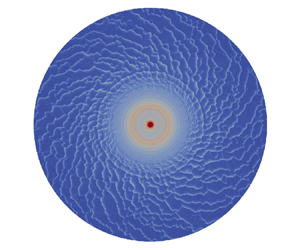
The investigation of a rotating film flow in this work accounts for the transition of wave regimes by considering the local flow rate $\hat {q}$, which significantly decreases as the film spreads outwards; see figure 3. Hence, we adopt the local Reynolds number $Re_{L}$ proportional to $\hat {q}$ to determine whether a region is subjected to laminar or turbulent conditions: $Re_{L} = \hat {q}/\hat {\nu }$. Specifically, $Re_{L}$ in proximity to the jet impingement point exceeds the criterion of transition from the laminar to turbulent regime given in previous studies on falling films, and so the region near the jet impingement is turbulent. By contrast, the downstream region with lower local flow rates (and local Reynolds numbers) is predominantly laminar. Consequently, to develop accurate IBL equations for a rotating film with three-dimensional solitary waves, it is essential to incorporate both laminar and turbulent models, taking into account the local Reynolds number.

Figure 3.

Time-averaged local Reynolds number $\langle Re_{L} \rangle$ with respect to radial position $\hat {r}$.

The concept of the turbulent regime in the film flow discussed in this study should not be confused with the wave turbulization proposed by Butuzov & Pukhovoi (Reference Butuzov and Pukhovoi1976). The term interfacial turbulence is commonly employed to describe the complex dynamics of solitary waves. As the system of solitary waves exhibits robust coherent structures, continuously interacting with each other as quasiparticles, it is often referred to as weak and dissipative turbulence (Denner et al. Reference Denner, Charogiannis, Pradas, Markides, van Wachem and Kalliadasis2018). Therefore, wave turbulization indicates the transformation of concentric waves into a group of three-dimensional waves exhibiting spatiotemporal chaos. The system of irregular solitary waves is typically associated with low-flow-rate conditions. By contrast, the turbulence discussed in this study emerges when the local flow rate is beyond the range in which solitary waves are observed. In this context, turbulence refers to a hydrodynamic state characterized by the presence of internal vortex structures (Hwang & Chang Reference Hwang and Chang1987; Adomeit & Renz Reference Adomeit and Renz2000) and the dominance of roll waves, along with a power-law velocity distribution in the vertical direction (Brauner Reference Brauner1989). This study emphasizes the presence of turbulent film flow in the upstream region where the local flow rate is large. The turbulent structures in the upstream region are correlated with the generation of chaotic solitary waves, known as wave turbulization, in the downstream region.

Before proceeding with integral modelling, it is crucial to understand the source of concentric waves in the upstream region. Although the exact mechanism remains unclear, it is widely accepted that various interfacial flow phenomena arising from different nozzle configurations affect the formation of concentric waves (Charwat et al. Reference Charwat, Kelly and Gazley1972). In this study the concentric waves in the upstream region are caused by shear-induced disturbances on the surface of the circular liquid jet prior to impingement. The inception of disturbances on the jet interface is related with turbulent jets that are characterized by the jet Reynolds number $4\hat {Q}/(\hat {\nu } {\rm \pi}\hat {d})$ exceeding approximately 4000 for a smooth circular nozzle (Lienhard Reference Lienhard2006). In the current study the liquid jets under consideration are turbulent, falling within the range of $4\hat {Q}/(\hat {\nu } {\rm \pi}\hat {d})=4200\unicode{x2013}21\,000$. For scenarios with smaller $\hat {Q}$ or $\hat {H}$, concentric waves can be suppressed according to Wang et al. (Reference Wang, Gu, Sun, Ling, Peng, Yang, Yuan, Du and Wu2023). The comprehensive analysis about the effect of disk angular velocity $\hat {\varOmega }$ on the initiation of concentric waves has not been conducted. Nevertheless, we assume that the effect of $\hat {\varOmega }$ is negligible for the following reasons. Generation of concentric waves in the impinging zone occurs before the interface is influenced by disk rotation, and the tangential velocity by disk rotation is small near the disk centre; the effect of $\hat {\varOmega }$ becomes significant only after the boundary layer merger ($\hat {r} > \hat {r}_{0}$). Moreover, concentric waves are observed on a liquid film even without disk rotation ($\hat {\varOmega }=0$) when a turbulent liquid jet impinges on a solid surface (Lienhard Reference Lienhard2006).

To investigate the effects of liquid jet disturbance, concentric waves are visualized in the upstream region under various nozzle heights (figure 4). The volume flow rate $\hat {Q}$ and disk angular velocity $\hat {\varOmega }$ are the same in all cases. As the vertical distance between the nozzle and the disk increases, concentric waves with larger amplitudes and wavelengths appear. Furthermore, the concentric waves exhibit greater azimuthal disturbances when the nozzle is placed closer to the disk. Previous studies reported that surface disturbances on circular liquid jets are significantly influenced by the distance from the nozzle (Lienhard, Liu & Gabour Reference Lienhard, Liu and Gabour1992; Bhunia & Lienhard Reference Bhunia and Lienhard1994). Thus, our experimental findings indicate that the concentric waves in the upstream region are induced by the temporal fluctuations of the impinging jet due to disturbances on the jet interface. The concentric waves are modelled with an oscillatory input, having statistical characteristics that match the results from the sensor experiment. The modelling of the oscillatory input is discussed in § 4.3.

Figure 4.

Formation of concentric surface waves in the upstream region under different nozzle heights $\hat {H}$; for all cases, $\hat {Q}= 16.7\,{\rm mL}\,{\rm s}^{-1}$ and $\hat {\varOmega }=52.4\,{\rm rad}\,{\rm s}^{-1}$. Results are shown for (a) $\hat {H}=40\,{\rm mm}$, (b) $\hat {H}=20\,{\rm mm}$, (c) $\hat {H}=15\,{\rm mm}$.

3.1. Integral formulation of governing equations

The film flow is described by mass and momentum conservation equations, with boundary conditions applied on the liquid–gas interface ($\hat {z}=\hat {h}$) and the disk surface ($\hat {z}=0$). The governing equations and boundary conditions are transformed into a set of depth-integrated equations, employing the methodology presented by Kim & Kim (Reference Kim and Kim2009) to derive IBL equations. As mentioned in § 2.1, the IBL equations presented below are applicable for $\hat {r}>\hat {r}_{0}$, irrespective of the local Reynolds number. To make the governing equations and boundary conditions dimensionless, the following normalization is adopted:

(3.1)\begin{equation} \left. \begin{aligned} r & = \frac{\hat{r}}{\hat{l}}, \quad z = \frac{\hat{z}}{\hat{\delta}}, \quad t = \frac{1}{\hat{\varOmega}},\\ u_{r} & = \frac{\hat{u}_{r}}{\hat{u}_{0}}, \quad u_{\theta} = \frac{\hat{u}_{\theta}}{\hat{u}_{0}}, \quad h = \frac{\hat{h}}{\hat{\delta}}, \quad u_{z} = \frac{\hat{u}_{z}}{\hat{\delta}\hat{\varOmega}}, \quad p = \frac{\hat{p}}{\hat{\rho}\hat{l}^{2}\hat{\varOmega}^{2}}. \end{aligned} \right\} \end{equation}

The dimensional pressure and time are denoted by $\hat {p}$ and $\hat {t}$, respectively. The characteristic length scales for the horizontal direction, $\hat {l}=(9\hat {Q}^{2}/ 4{\rm \pi} ^{2}\hat {\nu }\hat {\varOmega })^{1/4}$, and the vertical direction, $\hat {\delta }=(\hat {\nu }/\hat {\varOmega })^{1/2}$, are chosen following Rauscher, Kelly & Cole (Reference Rauscher, Kelly and Cole1973). The reference horizontal velocity $\hat {u}_{0}$ is defined as $\hat {l}\hat {\varOmega }$. For a detailed discussion on scaling parameters and normalization, see Kim & Kim (Reference Kim and Kim2009). The scaling proposed by Kim & Kim (Reference Kim and Kim2009), which uses a universal length scale for both the radial and azimuthal directions, is more suitable for modelling three-dimensional waves than scaling based on the Ekman number (Sisoev et al. Reference Sisoev, Matar and Lawrence2003). This is because the velocity fluctuations resulting from continuous interactions among solitary waves in the downstream region means that the velocity scale in the azimuthal direction is no longer distinct from that in the radial direction. The same scaling holds upstream because the influence of the inertia force surpasses that of the rotational body forces.

The governing equations and boundary conditions are formulated using the long-wave approach, which assumes that the ratio between the horizontal length scale $\hat {l}$ and the depth scale $\hat {\delta }$ is much smaller than unity. In this study a dimensionless long-wave parameter $\epsilon = \hat {\delta }/\hat {l} \ll 1$ is introduced. The product of $\epsilon$ and the global Reynolds number, defined as $Re_{G} = \hat {u}_{0}\hat {\delta }/\hat {\nu }$, is of order unity. The global Reynolds number, therefore, does not appear explicitly in the normalized governing equations and boundary conditions. The dimensionless governing equations in the reference frame rotating with the disk are then presented as

(3.2a)$$\begin{gather} \frac{1}{r}\frac{\partial}{\partial r}\left(ru_{r}\right)+\frac{1}{r}\frac{\partial u_{\theta}}{\partial \theta}+\frac{\partial u_{z}}{\partial z} =0, \end{gather}$$

(3.2b)$$\begin{gather} \frac{\partial u_{r}}{\partial t} + u_{r}\frac{\partial u_{r}}{\partial r} + \frac{u_{\theta}}{r}\frac{\partial u_{r}}{\partial \theta} + u_{z}\frac{\partial u_{r}}{\partial z} - \frac{u_{\theta}^{2}}{r} ={-} \frac{\partial p}{\partial r} + r + 2u_{\theta} + \frac{\partial^{2} u_{r}}{\partial z^{2}} \nonumber\\ +\ \epsilon^{2}\left(\frac{\partial^{2} u_{r}}{\partial r^{2}} + \frac{1}{r}\frac{\partial u_{r}}{\partial r} + \frac{1}{r^{2}}\frac{\partial^{2} u_{r}}{\partial \theta^{2}} - \frac{2}{r^{2}}\frac{\partial u_{\theta}}{\partial \theta} - \frac{u_{r}}{r^{2}}\right), \end{gather}$$

(3.2c)$$\begin{gather} \frac{\partial u_{\theta}}{\partial t} + u_{r}\frac{\partial u_{\theta}}{\partial r} + \frac{u_{\theta}}{r}\frac{\partial u_{\theta}}{\partial \theta} + u_{z}\frac{\partial u_{\theta}}{\partial z} + \frac{u_{r}u_{\theta}}{r} ={-} \frac{1}{r}\frac{\partial p}{\partial \theta} - 2u_{r} + \frac{\partial^{2} u_{\theta}}{\partial z^{2}} \nonumber\\ +\ \epsilon^{2}\left(\frac{\partial^{2} u_{\theta}}{\partial r^{2}} + \frac{1}{r}\frac{\partial u_{\theta}}{\partial r} + \frac{1}{r^{2}}\frac{\partial^{2} u_{\theta}}{\partial \theta^{2}} + \frac{2}{r^{2}}\frac{\partial u_{r}}{\partial \theta} - \frac{u_{\theta}}{r^{2}}\right), \end{gather}$$

(3.2d)$$\begin{gather} \epsilon^{2}\left(\frac{\partial u_{z}}{\partial t} + u_{r}\frac{\partial u_{z}}{\partial r} + \frac{u_{\theta}}{r}\frac{\partial u_{z}}{\partial \theta} + u_{z}\frac{\partial u_{z}}{\partial z}\right) ={-} \frac{\partial p}{\partial z} - \epsilon Fr^{{-}1} + \epsilon^{2}\frac{\partial^{2} u_{z}}{\partial z^{2}} \nonumber\\ +\ \epsilon^{4}\left(\frac{\partial^{2} u_{z}}{\partial r^{2}} + \frac{1}{r}\frac{\partial u_{z}}{\partial r} + \frac{1}{r^{2}}\frac{\partial^{2} u_{z}}{\partial \theta^{2}}\right), \end{gather}$$

where $Fr=\hat {\varOmega }^{2}\hat {l}/\hat {g}$ is the Froude number. Equation (3.2a) is the dimensionless continuity equation, whereas (3.2b–d) are the dimensionless momentum equations in the $r$, $\theta$ and $z$ directions, respectively.

The boundary condition on the disk surface ($z = 0$) is the no-slip condition, and the kinematic boundary condition is imposed on the film surface ($z = h$). The dimensionless forms of these boundary conditions are

(3.3a)$$\begin{gather} u_{r}=u_{\theta}=u_{z}=0,\quad \text{at} \ z=0, \end{gather}$$

(3.3b)$$\begin{gather}\frac{\partial h}{\partial t} + u_{r}\frac{\partial h}{\partial r} + \frac{u_{\theta}}{r}\frac{\partial h}{\partial \theta} = u_{z} ,\quad \text{at}\ z=h. \end{gather}$$

Tangential and normal stress balance conditions should also be imposed on the film surface ($z = h$). Here, the shear stress induced by the gas flow above the film surface is neglected (stress-free condition). These boundary conditions are

(3.4a)\begin{align} &\left(\epsilon^{2} \frac{\partial u_{z}}{\partial r} + \frac{\partial u_{r}}{\partial z}\right)\left[1 - \epsilon^{2}\left(\frac{\partial h}{\partial r}\right)^{2}\right] + 2\epsilon^{2}\left(\frac{\partial u_{z}}{\partial z} - \frac{\partial u_{r}}{\partial r}\right)\frac{\partial h}{\partial r} \nonumber\\ &\qquad-\epsilon^{2} \frac{1}{r}\frac{\partial h}{\partial \theta}\left[\frac{1}{r}\frac{\partial u_{r}}{\partial \theta} + \frac{\partial u_{\theta}}{\partial r} - \frac{u_{\theta}}{r} + \left(\frac{\partial u_{\theta}}{\partial z} + \epsilon^{2}\frac{1}{r}\frac{\partial u_{z}}{\partial \theta}\right)\frac{\partial h}{\partial r}\right] = 0,\quad \text{at} \ z = h, \end{align}

(3.4b)\begin{align} &\left(\epsilon^{2} \frac{1}{r}\frac{\partial u_{z}}{\partial \theta} + \frac{\partial u_{\theta}}{\partial z}\right)\left[1 - \epsilon^{2}\left(\frac{1}{r}\frac{\partial h}{\partial \theta}\right)^{2}\right] + 2\epsilon^{2}\left(\frac{\partial u_{z}}{\partial z} - \frac{1}{r}\frac{\partial u_{\theta}}{\partial \theta} - \frac{u_{r}}{r}\right)\frac{1}{r}\frac{\partial h}{\partial \theta} \nonumber\\ &\qquad-\epsilon^{2}\frac{\partial h}{\partial r}\left[\frac{1}{r}\frac{\partial u_{r}}{\partial \theta} + \frac{\partial u_{\theta}}{\partial r} - \frac{u_{\theta}}{r} + \left(\frac{\partial u_{r}}{\partial z} + \epsilon^{2}\frac{\partial u_{z}}{\partial r}\right)\frac{1}{r}\frac{\partial h}{\partial \theta}\right] = 0,\quad \text{at} \ z = h, \end{align}

(3.4c) \begin{align} &{-} p - \epsilon^{3}\kappa We + 2\epsilon^{2}\left[1 + \epsilon^{2}\left(\frac{\partial h}{\partial r}\right)^{2} + \frac{\epsilon^{2}}{r^{2}}\left(\frac{\partial h}{\partial \theta}\right)^{2}\right]^{{-}1} \nonumber\\ &\qquad \times \left[\frac{\partial u_{z}}{\partial z} - \left(\frac{\partial u_{r}}{\partial z} + \epsilon^{2}\frac{\partial u_{z}}{\partial r}\right)\frac{\partial h}{\partial r} + \epsilon^{2}\frac{\partial u_{r}}{\partial r}\left(\frac{\partial h}{\partial r}\right)^{2} - \left(\frac{\partial u_{\theta}}{\partial z} + \frac{\epsilon^{2}}{r}\frac{\partial u_{z}}{\partial \theta}\right)\frac{1}{r}\frac{\partial h}{\partial \theta}\right. \nonumber\\ &\qquad +\left. \epsilon^{2}\left(\frac{1}{r}\frac{\partial u_{r}}{\partial \theta} + \frac{\partial u_{\theta}}{\partial r} - \frac{u_{\theta}}{r}\right)\frac{1}{r}\frac{\partial h}{\partial \theta}\frac{\partial h}{\partial r} + \epsilon^{2}\left(\frac{1}{r}\frac{\partial u_{\theta}}{\partial \theta} + \frac{\partial u_{r}}{\partial r}\right)\frac{1}{r^{2}}\left(\frac{\partial h}{\partial \theta}\right)^{2} \right] = 0,\nonumber\\&\quad \text{at} \ z = h, \end{align}

where $\kappa$ denotes the mean curvature of the free surface and $We = \hat {\sigma }/\hat {\rho }\hat {\varOmega }^{2}\hat {l}\hat {\delta }^{2}$ is the Weber number. Boundary conditions (3.4a,b) concern the stress balance in the tangential direction, whereas (3.4c) is the stress balance in the normal direction. The unknown film thickness and small $\epsilon$ make numerical solutions from governing equations (3.2) subject to boundary conditions (3.3) and (3.4) challenging. Hence, the boundary layer approximation is introduced along with depth integration to simplify the equations.

Before the integral approach is employed to relate the film thickness $h$ with the horizontal velocity components $u_r$ and $u_\theta$, terms of $O(\epsilon ^{2})$ and higher orders are neglected in accordance with the first-order long-wave approximation. The stress-free boundary condition (3.4) then yields

(3.5a–c)\begin{equation} \left.\frac{\partial u_{r}}{\partial z}\right\rvert_{z = h} = 0, \quad \left.\frac{\partial u_{\theta}}{\partial z}\right\rvert_{z = h} = 0, \quad p\rvert_{z=h} ={-}\epsilon \kappa \mathbb{W}, \end{equation}

where $\mathbb {W} = \epsilon ^{2}We (= \hat {\sigma }/\hat {\rho }\hat {\varOmega }^{2}\hat {l}^{3})$. By applying the pressure on the free surface (3.5c) and the long-wave approximation ($\epsilon \ll 1$), the following pressure distribution is obtained by integrating the vertical component of the momentum balance equation (3.2d) from an arbitrary location $z$ to $z=h$ along the $z$ direction:

(3.6)\begin{equation} p ={-}\epsilon \kappa \mathbb{W} + \epsilon Fr^{{-}1}(h-z). \end{equation}

Incorporating the pressure equation (3.6), simplified stress-free boundary conditions (3.5a,b) and other boundary conditions (3.3), the continuity equation (3.2a) and momentum conservation equations in the $r$ and $\theta$ directions (3.2b,c) are integrated along the $z$ direction from $z=0$ to $z=h$ using the Leibniz integral rule. To facilitate the presentation of the integrated equations, we introduce the depth-averaged velocity components $\bar {u}_{r}(=({1}/{h})\int _0^h u_r\,\mathrm {d}z)$ and $\bar {u}_{\theta }(=({1}/{h})\int _0^h u_\theta \,\mathrm {d}z)$. Consequently, the depth-integrated equations, which establish the relationship between $h$, $\bar {u}_{r}$ and $\bar {u}_{\theta }$, are expressed as

(3.7a)$$\begin{gather} \frac{\partial h}{\partial t} + \frac{1}{r}\frac{\partial}{\partial r}(r\bar{u}_{r}h) + \frac{1}{r}\frac{\partial}{\partial \theta}(\bar{u}_{\theta}h) = 0, \end{gather}$$

(3.7b)$$\begin{gather} \frac{\partial \bar{u}_{r}h}{\partial t} + \frac{1}{r}\frac{\partial}{\partial r}(r\overline{u_{r}^{2}}h) + \frac{1}{r}\frac{\partial}{\partial \theta}(\overline{u_{r}u_{\theta}}h) - \frac{\overline{u_{\theta}^{2}}h}{r} ={-} \frac{\partial h\bar{p}}{\partial r} & + p\rvert_{z=h}\frac{\partial h}{\partial r} + rh \nonumber\\ & +\ 2 \bar{u}_{\theta}h -\left. \frac{\partial u_{r}}{\partial z}\right\rvert_{z=0}, \end{gather}$$

(3.7c)$$\begin{gather} \frac{\partial \bar{u}_{\theta}h}{\partial t} + \frac{1}{r}\frac{\partial}{\partial r}(r\overline{u_{r}u_{\theta}}h) + \frac{1}{r}\frac{\partial}{\partial \theta}(\overline{u_{\theta}^{2}}h) + \frac{\overline{u_{r}u_{\theta}}h}{r} & ={-} \frac{1}{r}\frac{\partial h\bar{p}}{\partial \theta} + p\rvert_{z=h}\frac{1}{r}\frac{\partial h}{\partial \theta} \nonumber\\ & -\ 2 \bar{u}_{r}h - \left.\frac{\partial u_{\theta}}{\partial z}\right\rvert_{z=0}, \end{gather}$$

(3.7d)$$\begin{gather}\bar{p} ={-}\epsilon\kappa\mathbb{W} + \frac{1}{2}\epsilon Fr^{{-}1} h, \end{gather}$$

where the terms $rh$, $2\bar {u}_{r}h$ and $2\bar {u}_{\theta }h$ on the right-hand side come from the centrifugal and Coriolis forces, respectively. The gravitational body force is incorporated into the pressure equation (3.7d) in terms of $Fr^{-1}$, which comes from (3.6). The mean curvature $\kappa$ of the free surface is expressed as $\kappa =\boldsymbol {\nabla } \boldsymbol {\cdot } [\boldsymbol {\nabla } h/(|\boldsymbol {\nabla }h|^{2}+1)^{1/2}]$. Here, the gradient operator $\boldsymbol {\nabla }$ is defined in the horizontal coordinates as $\boldsymbol {\nabla } = ({\partial }/{\partial r})\boldsymbol {e}_{r} + ({1}/{r})({\partial }/{\partial \theta })\boldsymbol {e}_{\theta }$.

The variables of the governing equations (3.7) are $h$, $\bar {u}_{r}$ and $\bar {u}_{\theta }$; the depth-averaged pressure $\bar {p}$ in (3.7d) is a function of $h$. Thus, the equations are not closed because of the convective terms ($\overline {u_{r}^{2}}$, $\overline {u_{r} u_{\theta }}$, $\overline {u_{\theta }^{2}}$) and bottom shear terms ($\partial u_{r}/\partial z\rvert _{z=0}$, $\partial u_{\theta }/\partial z\rvert _{z=0}$). In the Kapitza–Shkadov IBL equations, the convective and bottom shear terms are closed by assuming a self-similar velocity profile (Kalliadasis et al. Reference Kalliadasis, Ruyer-Quil, Scheid and Velarde2012). A specific form of the velocity profile enables the closure terms to be defined in terms of the film thickness and depth-averaged velocity components:

(3.8a–c)$$\begin{gather} \overline{u_{r}^{2}} = k_{A}\bar{u}_{r}^{2}, \quad \overline{u_{r}u_{\theta}} = k_{B}\bar{u}_{r}\,\bar{u}_{\theta}, \quad \overline{u_{\theta}^{2}} = k_{C}\bar{u}_{\theta}^{2}, \end{gather}$$

(3.8d,e)$$\begin{gather}\left.\frac{\partial u_{r}}{\partial z}\right\rvert_{z=0} = f_{r}\frac{\bar{u}_{r}}{h}, \quad \left.\frac{\partial u_{\theta}}{\partial z}\right\rvert_{z=0} = f_{\theta}\frac{\bar{u}_{\theta}}{h}. \end{gather}$$

Here $k_{A}$, $k_{B}$, $k_{C}$, $f_{r}$ and $f_{\theta }$ are constants determined by the velocity profile along the vertical direction. These closure models, based on a single self-similar polynomial velocity profile, have successfully predicted the laminar film flow up to the global Reynolds number $Re_{G} \approx 75$ in falling films (Demekhin et al. Reference Demekhin, Kalaidin, Kalliadasis and Vlaskin2007; Denner et al. Reference Denner, Charogiannis, Pradas, Markides, van Wachem and Kalliadasis2018). However, the velocity profile deviates from the polynomial distribution for $Re_{G} > O(10^{2})$, as mentioned in § 2.3. Given the high local flow rate in the region near the jet impingement zone, it is essential to encompass the vertical velocity profile under high-Reynolds-number conditions in the closure models.

In this study we propose that the velocity profile along the $z$ direction should be chosen locally at any instant, in terms of the local Reynolds number $Re_{L} = \hat {q}/\hat {\nu }$ based on the local horizontal flow rate. We can express $Re_{L}$, using the IBL equation variables $\hat {h}$ and $\bar {\hat {\boldsymbol {u}}}$ as

(3.9)\begin{equation} Re_{L}=\frac{\hat{h}\rvert\bar{\hat{\boldsymbol{u}}}\rvert}{\hat{\nu}}, \end{equation}

where $\bar {\hat {\boldsymbol {u}}}$ denotes the depth-averaged horizontal velocity vector in dimensional form: $({1}/{\hat {h}})\int _{0}^{\hat {h}} (\hat {u}_{r},\hat {u}_{\theta }) \,\mathrm {d}\hat {z}$. As mentioned in § 2.3, the flow field is divided into laminar and turbulent film flow based on the local Reynolds number $Re_{L}$. The critical Reynolds number $Re_{*}$, which acts as a threshold between these two regimes, is set to 100, following the criterion proposed by Mendez et al. (Reference Mendez, Gosset, Scheid, Balabane and Buchlin2021). Figure 5 conceptually illustrates velocity profiles in the laminar and turbulent film flow regimes. For regions with $Re_{L} \leq 100$, the closure models for the laminar film flow are based on a polynomial velocity profile. By contrast, a power-law velocity profile is used to describe turbulent film flow for regions with $Re_{L} > 100$, where sub-depth scale vortical structures emerge near the bottom.

Figure 5.

Schematics of velocity profiles along the vertical direction for two flow regimes based on the local Reynolds number $Re_{L}$. The solid line denotes the instantaneous velocity profile and the dashed line is the time-averaged velocity profile. Results are shown for (a) $Re_{L}\leq 100$ and (b) $Re_{L}>100$.

3.2. Closure model for laminar regime

In the laminar regime the closure terms are determined based on a self-similar polynomial velocity profile in the vertical direction. The shape of the velocity profile is considered to be independent of $Re_{L}$ in this regime, as experimentally verified under a low flow rate (Dietze, Al-sibai & Kneer Reference Dietze, Al-sibai and Kneer2009). The following velocity profile assumption introduced by Sisoev et al. (Reference Sisoev, Matar and Lawrence2003) in the Kapitza–Shkadov method for rotating films has been widely adopted: $u_{r} = 3\bar {u}_{r}(\eta - \tfrac {1}{2}\eta ^{2})$ and $u_{\theta } = 5\bar {u}_{\theta }\tfrac {1}{4}(2\eta - \eta ^{3} + \tfrac {1}{4}\eta ^{4})$, where $\eta = z/h$ varies from 0 to 1. The parabolic and quartic velocity profiles are obtained as asymptotic solutions of the governing equations in the limit of a large Ekman number (Shkadov Reference Shkadov1973). The primary assumption underlying the derivation of separate profiles in the $r$ and $\theta$ directions is the dominance of viscous and body forces over inertia forces. However, the present study is characterized by relatively large flow rates, so this assumption is no longer applicable. Thus, we suggest a single quartic velocity profile for both radial and tangential directions.

Both the radial and tangential velocity profiles are assumed to follow the quartic formulations

(3.10a)$$\begin{gather} u_{r}(r,\theta,z,t)=\frac{5}{4}\bar{u}_{r}(r,\theta,t)\left(2\eta-\eta^{3}+\frac{\eta^{4}}{4}\right), \end{gather}$$

(3.10b)$$\begin{gather}u_{\theta}(r,\theta,z,t)=\frac{5}{4}\bar{u}_{\theta}(r,\theta,t)\left(2\eta-\eta^{3}+\frac{\eta^{4}}{4}\right). \end{gather}$$

These velocity profiles satisfy the boundary conditions (3.3a) and (3.5a,b). Quartic profiles were partially adopted by Kim & Kim (Reference Kim and Kim2009), where the time-averaged film thickness acquired from the numerical results of IBL equations was found to be in good agreement with experimental results. A rationale behind adopting the quartic profile is extensively discussed in Appendix B. The closure terms in (3.8) for the laminar regime ($Re_{L} \leq Re_{*}$, where $Re_{*} = 100$) are calculated from (3.10) as

(3.11a,b)\begin{equation} k_{A}=k_{B}=k_{C}=k_{l}=\frac{155}{126}, \quad f_{r}=f_{\theta}=\frac{5}{2}, \end{equation}

where $k_{l}$ denotes the advection closure constant in the laminar regime.

Despite numerous benefits of using more advanced and complicated mathematical models, including the wall-resolved inner boundary layer approach that accurately predicts the threshold of linear stability, the Kármán–Pohlhausen-type integral approach employed in the present work is sufficient to capture the dynamics of three-dimensional solitary waves (Chang, Demekhin & Kopelevitch Reference Chang, Demekhin and Kopelevitch2006), which still remain elusive for rotating films. Moreover, it excels in integrating the power-law profiles in the high-$Re_{L}$ regime into the IBL framework.

3.3. Closure model for turbulent regime

Next, we present closure models for the turbulent regime ($Re_{L} > Re_{*}$). Analysis of the film flows in this regime often involves mixing length theory (King Reference King1966; Geshev Reference Geshev2014) and shallow-water assumptions (Mukhopadhyay, Chhay & Ruyer-Quil Reference Mukhopadhyay, Chhay and Ruyer-Quil2017; James et al. Reference James, Lagrée, Le and Legrand2019; Mendez et al. Reference Mendez, Gosset, Scheid, Balabane and Buchlin2021), as well as investigation of the characteristics of roll waves (Nakoryakov, Ostapenko & Bartashevich Reference Nakoryakov, Ostapenko and Bartashevich2012; Yu & Chu Reference Yu and Chu2022). Among these approaches, the one particularly suitable to IBL formulations is the shallow-water dynamics (James et al. Reference James, Lagrée, Le and Legrand2019). The shallow-water equations, which are derived through the long-wave approximation and depth averaging, exhibit compatibility with the framework of the present study. In turbulent shallow water, the power-law velocity profile is assumed instead of the polynomial profile. We refer to the shallow-water model proposed for liquid films undergoing jet wiping (Mendez et al. Reference Mendez, Gosset, Scheid, Balabane and Buchlin2021) and develop a turbulent closure model that is specifically tailored for rotating films. In addition to the velocity profile, the influence of sub-depth scale turbulent structures on the horizontal momentum balance, as suggested in studies on shallow-water flows, is also incorporated. Regarding film flows over a rotating disk, this is the first application of the shallow-water model to the IBL equations, to the best of our knowledge.

The turbulent flow requires the modelling of length scales to be divided into resolved and unresolved components. The resolved scales encompass greater horizontal flow structures, whereas the unresolved scales represent smaller internal structures. To address both scales, the velocity components are initially decomposed into filtered (resolved) and sub-grid scale (unresolved) components. This decomposition allows for the derivation of filtered versions of the depth-averaged equations, drawing inspiration from the literature on depth-averaged large-eddy simulations (DA LES) for turbulent shallow waters (Hinterberger et al. Reference Hinterberger, Fröhlich and Rodi2007; van Prooijen & Ujittewaal Reference van Prooijen and Ujittewaal2009). In these simulations, the grid size is typically comparable to the water depth, leading to the term sub-depth scale instead of sub-grid scale. The filtered velocity is then assumed to have a power-law profile along the vertical direction, which is used to derive the closure equations (3.8). As for the unfiltered components, sub-depth scale stress is interpreted as a random force vector field applied to the governing equations of the resolved scale, which is referred to as a stochastic backscatter model.

3.3.1. Filtered formulation

To capture the influence of turbulent structures, the concept of filtering, commonly used in DA LES, is introduced to the IBL formulation. Let us decompose the velocity vector $\boldsymbol {u} = (u_{r},u_{\theta },u_{z})$ into $\boldsymbol {u}=\tilde {\boldsymbol {u}}+\boldsymbol {u}'$, where $\tilde {\boldsymbol {u}}$ denotes the thickness-based Favre-filtered velocity $\tilde {\boldsymbol {u}} = \underline {h\boldsymbol {u}}/\underline {h}$; the underline marker ($\underline {\cdot }$) denotes a spatial filter $\underline {\varphi }(\boldsymbol {x})= \int _D \varphi (\boldsymbol {x}')G(\boldsymbol {x}'-\boldsymbol {x}) \,\textrm {d}\,\boldsymbol {x}'$ (Hinterberger et al. Reference Hinterberger, Fröhlich and Rodi2007). The pressure is similarly decomposed. Filtering the continuity and horizontal momentum equations (3.2a–c) yields

(3.12a)$$\begin{gather} \frac{1}{r}\frac{\partial}{\partial r}(r\tilde{u}_{r})+\frac{1}{r}\frac{\partial \tilde{u}_{\theta}}{\partial \theta}+\frac{\partial \tilde{u}_{z}}{\partial z}=0, \end{gather}$$

(3.12b)$$\begin{gather}\frac{\partial \tilde{u}_{r}}{\partial t} + \frac{\partial \widetilde{u_{r}^{2}}}{\partial r} + \frac{1}{r}\frac{\partial \widetilde{u_{r}u_{\theta}}}{\partial \theta} + \frac{\partial \widetilde{u_{r}u_{z}}}{\partial z} - \frac{\widetilde{u_{r}^{2}}-\widetilde{u_{\theta}^{2}}}{r} ={-} \frac{\partial \tilde{p}}{\partial r} + r + 2\tilde{u}_{\theta} + \frac{\partial^{2} \tilde{u}_{r}}{\partial z^{2}}, \end{gather}$$

(3.12c)$$\begin{gather}\frac{\partial \tilde{u}_{\theta}}{\partial t} + \frac{\partial \widetilde{u_{\theta}u_{r}}}{\partial r} + \frac{1}{r}\frac{\partial \widetilde{u_{\theta}^{2}}}{\partial \theta} + \frac{\partial \widetilde{u_{\theta}u_{z}}}{\partial z} + \frac{2\widetilde{u_{r}u_{\theta}}}{r} ={-} \frac{1}{r}\frac{\partial \tilde{p}}{\partial \theta} - 2\tilde{u}_{r} + \frac{\partial^{2} \tilde{u}_{\theta}}{\partial z^{2}}, \end{gather}$$

where the long-wave approximation still holds for the filtered velocity scales. By applying the Favre-filtering technique to the governing momentum equation in the $z$ direction (3.2d) and the corresponding boundary conditions (3.3) and (3.4), the velocity and pressure terms of $O(\epsilon ^{2})$ and lower are replaced with their respective Favre-filtered variables. Consequently, the filtered vertical momentum equation and boundary conditions yield the filtered pressure, which is equivalent to (3.6) with $h$ replaced by $\underline{h}$:

(3.13)\begin{equation} \tilde{p} ={-} \epsilon \tilde{\kappa} \mathbb{W} + \epsilon Fr^{{-}1} (\underline{h}-z). \end{equation}

Here $\tilde {\kappa } = \boldsymbol {\nabla } \boldsymbol {\cdot } [\boldsymbol {\nabla } \underline {h}/ (\rvert \boldsymbol {\nabla } \underline {h} \rvert ^{2}+1)^{1/2}]$.

In the filtered equations (3.12), all terms except advection terms are expressed with $\tilde {u}_{r}, \tilde {u}_{\theta }, \tilde {u}_{z}$ and $\tilde {p}$. The distinction between the filtered advection and the advection of the filtered velocity, denoted as $\partial (\widetilde {u_{i}u_{j}} - \tilde {u}_{i}\tilde {u}_{j})/\partial x_{j}$ in Cartesian tensor notation, plays a crucial role in LES, giving rise to the concepts of sub-grid scale stress and eddy viscosity. In the present work, the filtered velocity products $\widetilde {u_{r}^{2}}, \widetilde {u_{\theta }^{2}}, \widetilde {u_{r}u_{\theta }}, \widetilde {u_{r}u_{z}}, \widetilde {u_{\theta }u_{z}}$ are likewise decomposed into $\tilde {u}_{r}^{2}, \tilde {u}_{\theta }^{2}, \tilde {u}_{r}\tilde {u}_{\theta }, \tilde {u}_{r}\tilde {u}_{z}, \tilde {u}_{\theta }\tilde {u}_{z}$ and the sub-grid scale stress terms $(\widetilde {u_{i}u_{j}} - \tilde {u}_{i}\,\tilde {u}_{j})$.

Following previous studies on shallow-water LES (Nadaoka & Yagi Reference Nadaoka and Yagi1998; Hinterberger et al. Reference Hinterberger, Fröhlich and Rodi2007), the Favre-filtered velocity components are interpreted as being grid resolved, and are considered identical to the velocity components without filtering in the laminar regime. The scaling parameters in (3.1) and the local Reynolds number in (3.9) are defined based on the grid-resolved values. Assuming identical vertical velocity profiles for $\tilde {u}_{r}$ and $\tilde {u}_{\theta }$, the depth integration of (3.12) using the pressure equation (3.13) and boundary conditions leads to a set of first-order long-wave boundary layer equations. The governing equations are expressed in Cartesian tensor notation to maintain consistency with existing LES formulations. Additionally, describing small-scale turbulence near the disk surface is challenging within the framework of cylindrical coordinates. The depth-integrated governing equations are

(3.14a)$$\begin{gather} \frac{\partial \underline{h}}{\partial t}+\frac{\partial }{\partial x_{i}} (\underline{h} \bar{\tilde{u}}_{i})=0, \end{gather}$$

(3.14b)$$\begin{gather} \frac{\partial (\underline{h} \bar{\tilde{u}}_{i})}{\partial t} + k_{t}\frac{\partial}{\partial x_{j}} (\underline{h} \bar{\tilde{u}}_{i}\,\bar{\tilde{u}}_{j}) & ={-} \frac{\partial \underline{h} \bar{\tilde{p}}}{\partial x_{i}} - \epsilon \tilde{\kappa} \mathbb{W}\frac{\partial \underline{h}}{\partial x_{i}} - \frac{\partial}{\partial x_{j}}(\underline{h} G_{ij}) \nonumber\\ & -\ \frac{1}{2}C_{f}\bar{\tilde{u}}_{i} \left(\bar{\tilde{u}}_{i}^{2} + \bar{\tilde{u}}_{j}^{2}\right)^{1/2} + B_{i}, \end{gather}$$

(3.14c)$$\begin{gather} \bar{\tilde{p}} ={-}\epsilon \tilde{\kappa} \mathbb{W} + \frac{1}{2} \epsilon Fr^{{-}1}\underline{h}, \end{gather}$$

where $(i,j = x,y)$ and $B_{i}$ indicates filtered and depth-integrated body forces (centrifugal force and Coriolis force terms). The depth-integrated pressure $\bar {\tilde {p}}$ in (3.14c) is obtained from (3.6), with unfiltered values replaced by filtered ones.

The constant $k_{t}$ in the advection term of (3.14b) is related to the assumption of a specific profile for the grid-resolved velocity in the vertical direction, which corresponds to (3.8a–c) and (3.11a) for the laminar regime. Here $k_{t}$ is equivalent to the constants $k_{A}$, $k_{B}$ and $k_{C}$; i.e. $k_{t}\bar {\tilde {u}}_{i} \,\bar {\tilde {u}}_{j} = \overline {\tilde {u}_{i} \tilde {u}_{j}}$. The fourth term on the right-hand side of (3.14b) represents bottom friction, which corresponds to the friction closure terms in (3.8d,e) and (3.11b) for the laminar regime. The determination of the closure models for $k_{t}$ and $C_{f}$ relies on the selection of the resolved velocity profile in the vertical direction, which is depicted in § 3.3.2. Additionally, $G_{ij}$ on the right-hand side, defined as $G_{ij} = \overline {\widetilde {u_{i}u_{j}}} - \overline {\tilde {u}_{i}\tilde {u}_{j}}$, represents the sub-grid scale stress arising from the filtering operator. This closure term for the sub-grid scale is modelled as a random force field using the stochastic backscatter model. The procedure for deriving the random force term is described in § 3.3.3.

3.3.2. Closure model for resolved velocity

The closure terms $k_{t}$ and $C_{f}$ in (3.14) are formulated based on assumptions regarding the resolved (filtered) velocity profile. The friction coefficient $C_f$ is inversely proportional to $Re_{L}$ in the laminar regime ($Re_L \leq Re_{*}$); $C_{f} = 5/Re_{L}$. For the turbulent regime ($Re_L > Re_{*}$), the friction coefficient is also regarded as a function of $Re_{L}$, exhibiting continuity with the laminar model at $Re_{L} = Re_{*}$, as suggested by Mendez et al. (Reference Mendez, Gosset, Scheid, Balabane and Buchlin2021). Specifically, we adopt an empirical relation of the form $C_{f} \approx a Re_{L}^{b}$, where $b \approx -1/4$ has been documented in studies of turbulent lubrication films (Elrod & Ng Reference Elrod and Ng1967; Hirs Reference Hirs1973). To ensure continuity at the transition point $Re_{*}$, the following expressions are proposed for the friction coefficients of the laminar and turbulent regimes:

(3.15)\begin{equation} C_{f} = \begin{cases} 5/Re_{L}, & Re_{L} \leq Re_{*}, \\ 5/(Re_{L}^{1/4}Re_*^{3/4}), & Re_{L} > Re_{*}. \end{cases} \end{equation}

The trend of $C_{f}$ in the vicinity of the transition regime is depicted in figure 6(a).

Figure 6.

(a) Trends of friction coefficient $C_f$ with respect to local Reynolds number $Re_L$ ($Re_{*}=100$). (b) Vertical velocity profiles for different local Reynolds numbers ($n_{T}=21$). The subscript $i (= x,y)$ indicates each horizontal direction.

To determine the closure terms for advection, it is crucial to establish a self-similar velocity profile, as outlined in § 3.2. To address transition from laminar to turbulent flow, the combination of the polynomial profile and the power-law profile, which represent the laminar and turbulent regimes, respectively, can be considered (Mendez et al. Reference Mendez, Gosset, Scheid, Balabane and Buchlin2021). As the local Reynolds number increases, the turbulent component becomes more dominant. The following mathematical expressions give the velocity profiles for the turbulent regime:

(3.16a) \begin{align} \tilde{u}_{x}(x,y,z,t)&=a_{L}\bar{\tilde{u}}_{x}(x,y,t)\left[\left(\frac{z}{\underline{h}}\right)-\frac{1}{2}\left(\frac{z}{\underline{h}}\right)^{3}+\frac{1}{8}\left(\frac{z}{\underline{h}}\right)^{4}\right] \nonumber \\ &\quad+ a_{T}\bar{\tilde{u}}_{x}(x,y,t)\left[\vphantom{\left(\frac{z}{\underline{h}}\right)-\frac{1}{2}\left(\frac{z}{\underline{h}}\right)^{3}+\frac{1}{8}\left(\frac{z}{\underline{h}}\right)^{4}}\left(\frac{z}{\underline{h}}-1\right)^{n_{T}}+1\vphantom{\left(\frac{z}{\underline{h}}\right)-\frac{1}{2}\left(\frac{z}{\underline{h}}\right)^{3}+\frac{1}{8}\left(\frac{z}{\underline{h}}\right)^{4}}\right], \end{align}

(3.16b) \begin{align} \tilde{u}_{y}(x,y,z,t)&=a_{L}\bar{\tilde{u}}_{y}(x,y,t)\left[\left(\frac{z}{\underline{h}}\right)-\frac{1}{2}\left(\frac{z}{\underline{h}}\right)^{3}+\frac{1}{8}\left(\frac{z}{\underline{h}}\right)^{4}\right] \nonumber\\ &\quad+ a_{T}\bar{\tilde{u}}_{y}(x,y,t)\left[\vphantom{\left(\frac{z}{\underline{h}}\right)-\frac{1}{2}\left(\frac{z}{\underline{h}}\right)^{3}+\frac{1}{8}\left(\frac{z}{\underline{h}}\right)^{4}}\left(\frac{z}{\underline{h}}- 1\right)^{n_{T}}+1\vphantom{\left(\frac{z}{\underline{h}}\right)-\frac{1}{2}\left(\frac{z}{\underline{h}}\right)^{3}+\frac{1}{8}\left(\frac{z}{\underline{h}}\right)^{4}}\right]. \end{align}

Here $a_{L}$ and $a_{T}$ are the superposition constants determined by the local flow rate per unit width and the friction coefficient. The polynomial component is identical to (3.10), so the profile is continuous at $Re_{L}=Re_{*}$ or, equivalently, $a_{L}=5/2, a_{T}=0$.

The velocity profile suggested in (3.16) should satisfy the following two conditions. First, the integration of the horizontal velocity from the bottom to the free surface $(({1}/{\underline {h}})\int _{0}^{\underline {h}}\tilde {u}_{i}\,\textrm {d}z)$ should yield the depth-averaged velocity $\bar {\tilde {u}}_{i}$; second, the bottom slope $\partial \tilde {u}_{i}/\partial z\rvert _{z=0}$ should match the friction coefficient $C_{f}$ given in (3.15). These constraints lead to the following expressions for the constants $a_{L}$ and $a_{T}$:

(3.17a)$$\begin{gather} a_{L}=\frac{5\left(n_{T}+1-\dfrac{1}{2}Re_{L}C_{f}\right)}{2n_{T}-3}, \end{gather}$$

(3.17b)$$\begin{gather}a_{T}=\frac{(n_{T}+1)\left(\dfrac{1}{2}Re_{L}C_{f}-5\right)}{n_{T}(2n_{T}-3)}. \end{gather}$$

As the local Reynolds number $Re_{L}$ continues to increase beyond $Re_{*}$, the profile gradually approaches the power-law profile. The velocity should increase monotonically along the $z$ direction, and the maximum velocity should be attained at $z = \underline {h}$. These conditions impose a physical constraint that determines the valid ranges of $a_{T}$ and $a_{L}$, thereby bounding the admissible limit of $Re_{L}$ based on (3.15) and (3.17). Moreover, choosing a larger value for $n_{T}$ tends to increase the maximum admissible value of $Re_{L}$. Thus, $n_{T} = 21$ is adopted because the range of $Re_{L}$ spans $O(10^{3})$ in the present work. More details on the choice of $n_{T}$ and the valid range of $Re_{L}$ have been described by Mendez et al. (Reference Mendez, Gosset, Scheid, Balabane and Buchlin2021). The resulting velocity profile applied in this work is presented in figure 6(b). From $k_{t}\bar {\tilde {u}}_{i} \,\bar {\tilde {u}}_{j} = \overline {\tilde {u}_{i} \tilde {u}_{j}}$, the advection constant $k_{t}$ in (3.14b) is expressed as

(3.18)\begin{equation} k_{t}=\frac{62}{315}a_{L}^{2}+\frac{9107}{22880}a_{L}a_{T}+\frac{441}{473}a_{T}^{2}. \end{equation}

3.3.3. Sub-depth scale turbulence model

In the field of shallow-water turbulence, the eddy scale of turbulent structures is typically divided into two ranges: three-dimensional structures of sub-depth scale and horizontal structures of large scale (Nadaoka & Yagi Reference Nadaoka and Yagi1998). One intriguing aspect of the coexistence of two-range length scales is the phenomenon of an inverse energy cascade in the spectral domain, also known as backscatter. This involves the transfer of energy from small three-dimensional eddies to large two-dimensional eddies. This backscattering process triggers the development of small-scale instabilities into large-scale horizontal motions (Hinterberger et al. Reference Hinterberger, Fröhlich and Rodi2007). Given the feature of long waves in film flows, it is reasonable to expect these two-range eddies to play a dominant role in the film flows. The backscatter effect is modelled as a random force field, i.e. stochastic backscatter model, as suggested by Hinterberger et al. (Reference Hinterberger, Fröhlich and Rodi2007). Therefore, this study incorporates a random force vector term into the closure process for the sub-depth scale stress $G_{ij}$ in (3.14b), which accounts for the influence of the inverse cascade.

In the context of DA LES models used in shallow-water turbulence, backscatter modelling is typically conducted for the total stress term (Nadaoka & Yagi Reference Nadaoka and Yagi1998; Hinterberger et al. Reference Hinterberger, Fröhlich and Rodi2007), rather than $G_{ij}$. The total stress $T_{ij} = \overline {\widetilde {u_{i}u_{j}}} - \bar {\tilde {u}}_{i}\, \bar {\tilde {u}}_{j}$ represents the unresolved stress resulting from depth-averaging ($\overline {\tilde {u}_{i}\tilde {u}_{j}} - \bar {\tilde {u}}_{i}\, \bar {\tilde {u}}_{j}$) added to $G_{ij} = \overline {\widetilde {u_{i}u_{j}}} - \overline {\tilde {u}_{i}\tilde {u}_{j}}$; note that $G_{ij}$ arises solely from the filtering operator. In many turbulent shallow-water models, where the time-averaged velocity is approximately constant along the vertical direction, except near solid surfaces, the effect of the depth-averaging operator ($\overline {\tilde {u}_{i}\tilde {u}_{j}} - \bar {\tilde {u}}_{i}\, \bar {\tilde {u}}_{j}$) is often neglected. However, in the present study we consider its influence through the advection closure constant $(k_{t}-1)\bar {\tilde {u}}_{i}\, \bar {\tilde {u}}_{j}(=\overline {\tilde {u}_{i}\tilde {u}_{j}} - \bar {\tilde {u}}_{i}\, \bar {\tilde {u}}_{j})$, as the effect of the velocity profile is deemed significant in rotating films. Therefore, the term $G_{ij} = T_{ij} - (\overline {\tilde {u}_{i}\tilde {u}_{j}} - \bar {\tilde {u}}_{i}\, \bar {\tilde {u}}_{j})$ arises in (3.14b) instead of $T_{ij}$.

First, we describe the decomposition of the total stress $T_{ij}$. The Favre filter is assumed to be separable to enable $\bar {\tilde {\phi }} \approx \tilde {\bar {\phi }}$. Then, the approximation

(3.19)\begin{equation} T_{ij}(=G_{ij} + \overline{\tilde{u}_{i}\tilde{u}_{j}} - \bar{\tilde{u}}_{i}\,\bar{\tilde{u}}_{j})=\overline{\widetilde{u_{i}u_{j}}} - \bar{\tilde{u}}_{i}\,\bar{\tilde{u}}_{j}\approx \widetilde{\overline{u_{i}u_{j}}} - \tilde{\bar{u}}_{i}\,\tilde{\bar{u}}_{j}\qquad (i,j=x,y) \end{equation}

holds, which is exact on the bottom of the disk and the free surface. Equation (3.19) is then decomposed into

(3.20)\begin{equation} (\widetilde{\overline{u_{i}u_{j}}} - \widetilde{\bar{u}_{i}\,\bar{u}_{j}})+(\widetilde{\bar{u}_{i}\,\bar{u}_{j}}-\tilde{\bar{u}}_{i}\,\tilde{\bar{u}}_{j}) =\tilde{D}_{ij}(\boldsymbol{u})+(\widetilde{\bar{u}_{i}\,\bar{u}_{j}}- \tilde{\bar{u}}_{i}\,\tilde{\bar{u}}_{j}), \end{equation}

where the second term $(\widetilde {\bar {u}_{i}\,\bar {u}_{j}}- \tilde {\bar {u}}_{i}\,\tilde {\bar {u}}_{j})$ corresponds to the sub-grid scale stress induced by filtering depth-averaged velocity components, which is typically modelled using eddy viscosity in studies on conventional two-dimensional turbulence (Nadaoka & Yagi Reference Nadaoka and Yagi1998; Hinterberger et al. Reference Hinterberger, Fröhlich and Rodi2007). The effect of three-dimensional sub-grid scale turbulence is included in the first term $\tilde {D}_{ij}(\boldsymbol {u})$, where $D_{ij}(\boldsymbol {u})$ is defined as

(3.21)\begin{equation} D_{ij}(\boldsymbol{u})=\frac{1}{\underline{h}}\int_{0}^{\underline{h}}(u_{i}-\bar{u}_{i})(u_{j}-\bar{u}_{j})\,{\rm d}z. \end{equation}

To further decompose the sub-grid scale stress $\tilde {D}_{ij}(\boldsymbol {u})$ in (3.20), we consider splitting the instantaneous velocity $\boldsymbol {u}$ into the time-averaged component $\langle \boldsymbol {u} \rangle$ and the fluctuating component $\boldsymbol {u}'$, where the notation $\langle \boldsymbol {\cdot } \rangle$ represents the time-averaging operator. Then, from (3.21), the decomposition is

(3.22)\begin{equation} \langle D_{ij}(\boldsymbol{u}) \rangle=D_{ij}(\langle\boldsymbol{u}\rangle)+\langle\overline{u_{i}'u_{j}'}\rangle-\langle\overline{u_{i}'}\,\overline{u_{j}'}\rangle=D_{ij}(\langle\boldsymbol{u}\rangle)+\langle D_{ij}(\boldsymbol{u}')\rangle. \end{equation}

Here, $\langle \overline {u'_{i}u'_{j}}\rangle$ represents the depth-averaged Reynolds stresses of all turbulent structures, and $\langle \overline {u_{i}'}\,\overline {u_{j}'}\rangle$ is the amount of stress caused by the horizontal flow structures of all scales. Thus, the difference between them, namely $\langle D_{ij}(\boldsymbol {u}')\rangle$, indicates the Reynolds stresses induced by three-dimensional fluctuations only. Given that Favre filtering separates the flow structures into fluctuations and large-scale resolved structures, we find the decomposition presented in (3.22) to be approximately valid for $\tilde {D}_{ij}(\boldsymbol {u})$:

(3.23)\begin{equation} \tilde{D}_{ij}(\boldsymbol{u})\approx D_{ij}(\tilde{\boldsymbol{u}}) + \tilde{D}_{ij}(\boldsymbol{u}'). \end{equation}

The first term $D_{ij}(\tilde {\boldsymbol {u}})$ on the right-hand side of (3.23) is equivalent to the stress induced by depth-averaging ($\overline {\tilde {u}_{i}\tilde {u}_{j}} - \bar {\tilde {u}}_{i}\,\bar {\tilde {u}}_{j}$) on the left-hand side of (3.19). Thus, from (3.20) and (3.23), $G_{ij}$ can be approximated as

(3.24)\begin{align} G_{ij} &\approx \tilde{D}_{ij}(\boldsymbol{u}') + (\widetilde{\bar{u}_{i}\,\bar{u}_{j}}- \tilde{\bar{u}}_{i}\,\tilde{\bar{u}}_{j})\nonumber\\ &\approx \tilde{D}_{ij}(\boldsymbol{u}') - \nu_{t}2\bar{\tilde{S}}_{ij}. \end{align}

The first term on the right-hand side of (3.24), $\tilde {D}_{ij}(\boldsymbol {u}')$, represents the sub-grid scale stress generated by three-dimensional turbulent structures near the disk surface (see figure 5b). The loss of information during depth-averaging and Favre filtering means that we must construct $\tilde {D}_{ij}(\boldsymbol {u}')$. In this study a stochastic backscatter model is applied to incorporate a random two-dimensional force vector field $F_{i,bsm}$, which is based on DA LES for shallow-water turbulence (Hinterberger et al. Reference Hinterberger, Fröhlich and Rodi2007). The second term, $(\widetilde {\bar {u}_{i}\,\bar {u}_{j}} - \tilde {\bar {u}}_{i}\,\tilde {\bar {u}}_{j})$, represents the unresolved stress typically used in LES, where the velocity components are replaced with the depth-averaged velocity and modelled using eddy viscosity, i.e. $-\nu _{t}2\bar{\tilde{S}}_{ij}$; the strain rate $S_{ij}$ is $\tfrac {1}{2}(\partial u_{i} / \partial x_{j} + \partial u_{j}/\partial x_{i})$. The eddy viscosity is commonly represented as $\nu _{t}=C\underline {h}\tilde {u}_{\tau }$, where $u_{\tau }$ denotes the friction velocity and $C$ is an empirical constant. The multiplication of the eddy viscosity and the strain rate, $\nu _{t}\bar {\tilde {S}}_{ij}$, is of $O(\epsilon ^{2})$ when differentiated with respect to the horizontal length scale, as discussed earlier for the long-wave formulation. Thus, the sub-grid scale stress term in (3.14) can be simplified to a random backscatter as follows:

(3.25)\begin{equation} \frac{\partial}{\partial x_{j}}(G_{ij}) ={-} F_{i,bsm} \quad (i,j=x,y). \end{equation}

The backscatter forcing term is linked to local turbulence production, which characterizes the dynamics of internal turbulent structures, and it is challenging to describe the backscattering of three-dimensional turbulence in terms of the long-wave scaling approach. Therefore, modelling the backscatter term requires expressions using dimensional parameters. We consider the dimensional $\hat {F}_{i,bsm} = \hat {l}\hat {\varOmega }^{2} F_{i,bsm}$, where $\hat {l}$ represents the horizontal length scale ($\hat {l}=(9\hat {Q}^{2}/ 4{\rm \pi} ^{2}\hat {\nu }\hat {\varOmega })^{1/4}$). The random force vector defined over the two-dimensional Cartesian coordinate system is

(3.26)\begin{equation} \hat{\boldsymbol{F}}_{bsm} = [\hat{\boldsymbol{\nabla}} \times (\hat{F}_{rms}Z \boldsymbol{e}_{z})] \hat{\varDelta} , \end{equation}

where the scalar value $\hat {F}_{rms}$ represents the root mean square of the backscatter force. To generate the backscatter forcing term, we introduce a filtered random scalar field $Z$ with zero mean and a normal distribution. A random force vector on the two-dimensional domain is constructed by the operator $\hat {\boldsymbol {\nabla }} = (\partial / \partial \hat {x}, \partial / \partial \hat {y})$. To ensure a divergence-free random vector field, the curl operator is applied to a vertically defined scalar field $\hat {F}_{rms}Z \boldsymbol {e}_{z}$. The solenoidal field introduced in (3.26), which pertains to the two-dimensional domain, is equivalent to the random vector potential field method used in three-dimensional backscatter models (Leith Reference Leith1990; Schumann Reference Schumann1995). The reference grid length scale $\hat {\varDelta }$ in (3.26) is obtained by averaging the grid sizes of the entire domain.

The scaling factor $\hat {F}_{rms}$ in (3.26) is derived from the two-dimensional production of turbulent kinetic energy, $\hat {P}_{2D}$: $\hat {P}_{2D} \sim \hat {F}_{rms}^{2} {\cdot } \Delta \hat {t}$, where $\Delta \hat {t}$ is the applied time step (Alvelius Reference Alvelius1999). Here $\hat {P}_{2D}$ scales as

(3.27)\begin{equation} \hat{P}_{2D} \sim \frac{\hat{P}_{3D}}{Re_{\tau}}=\frac{\rvert \bar{\tilde{\hat{\boldsymbol{u}}}} \rvert^{2}\hat{\nu}{C_{f}}^{1/2}}{\hat{\underline{h}}^{2}}, \end{equation}

where $\hat {P}_{3D}$ represents the three-dimensional turbulence production induced from bottom friction, and $Re_{\tau }=\hat {u}_{\tau }\hat {\underline {h}}/\hat {\nu }$ is the Reynolds number defined in terms of the friction velocity $\hat {u}_{\tau } = \rvert \bar {\tilde {\hat {\boldsymbol{u}}}} \rvert (C_{f}/2 )^{1/2}$. Hence, $\hat {F}_{rms}$ is updated every time step as

(3.28)\begin{equation} \hat{F}_{rms}=c_{B}\left(\frac{\hat{P}_{2D}}{\Delta \hat{t}}\right)^{1/2}=c_{B}\frac{\rvert\bar{\tilde{\hat{\boldsymbol{u}}}}\rvert C_{f}^{1/4}}{\hat{\underline{h}}}\left(\frac{\hat{\nu}}{\Delta \hat{t}}\right)^{1/2}, \end{equation}

where the empirical backscatter constant $c_{B} = 2.0$ is determined by comparing numerical results with experimental results obtained from sensor measurements. The effects of $c_{B}$ on the wave dynamics and local thickness of the liquid film are reported in § 5.2, along with a justification for the choice of $c_{B} = 2.0$.

4.1. Solver for IBL equations

Equations (3.7) and (3.14) for the laminar and turbulent regimes, respectively, are combined into a single set of equations. The combined equations are mathematically expressed in Cartesian tensor notation as follows:

(4.1a)$$\begin{gather} \frac{\partial \hat{h}}{\partial \hat{t}}+\frac{\partial}{\partial \hat{x}_{i}}(\hat{h} \bar{\hat{u}}_{i}) =0, \end{gather}$$

(4.1b)$$\begin{gather} \frac{\partial (\hat{h}\bar{\hat{u}}_{i})}{\partial \hat{t}} + \mathcal{K}\frac{\partial (\hat{h}\bar{\hat{u}}_{i}\,\bar{\hat{u}}_{j})}{\partial \hat{x}_{j}} & ={-}\frac{1}{\hat{\rho}}\frac{\partial(\hat{h} \bar{\hat{p}})}{\partial \hat{x}_{i}} - \frac{\hat{\sigma}\hat{\kappa}}{\hat{\rho}}\frac{\partial \hat{h}}{\partial \hat{x}_{i}} + \mathcal{L}\hat{h}\hat{F}_{i,bsm} \nonumber\\ & -\ \frac{1}{2}C_{f}\bar{\hat{u}}_{i}\left( \bar{\hat{u}}_{i}^{2} + \bar{\hat{u}}_{j}^{2} \right)^{1/2} + B_{i}, \end{gather}$$

(4.1c)$$\begin{gather} \bar{\hat{p}} ={-}\hat{\sigma}\hat{\kappa} + \frac{\hat{\rho}\hat{g}\hat{h}}{2} \quad (i,j = x,y). \end{gather}$$

In (4.1) the depth-averaged velocity $\bar {\hat {u}}_{i}$ and film thickness $\hat {h}$ are considered as resolved (filtered) values in the turbulent regime ($\bar {\hat {u}}_{i} \rightarrow \bar {\tilde {\hat {u}}}_{i}, \hat {h} \rightarrow \hat {\underline {h}}$), whereas they are equivalent to the original (unfiltered) values in the laminar regime. The backscatter force term $\hat {F}_{i,bsm}$ solely represents the sub-grid scale stress.

The closure models discussed in §§ 3.2 and 3.3 are combined into the constants $\mathcal {K}$, $\mathcal {L}$ and $C_{f}$. The values of these constants are determined based on the local Reynolds number $Re_{L}$ in each cell at each time step:

(4.2)\begin{equation} \left. \begin{array}{@{}ll@{}} \mathcal{L}=0,\mathcal{K} = k_{l},C_{f} = 5/Re_{L}, & Re_{L} \leq Re_{*}, \\ \mathcal{L}=1,\mathcal{K} = k_{t},C_{f} = 5/(Re_{L}^{1/4}Re_{*}^{3/4}), & Re_{L} > Re_{*}. \end{array} \right\} \end{equation}

By substituting the constants for the laminar regime ($Re_{L} \leq Re_{*}$) into (4.1), we obtain the Kapitza–Shkadov equations featuring the quartic velocity profiles, as suggested in § 3.2. When the constants for $Re_{L} > Re_{*}$ are used, the governing equations are transformed into the shallow-water DA LES equations discussed in § 3.3.

4.2. Computational domain and discretization

To solve (4.1), the implicit and sequential finite area solver proposed by Rauter & Tuković (Reference Rauter and Tuković2018) is employed. This finite area solver is known for accurately capturing the depth-averaged velocity and film thickness of two-dimensional flows. The fluid domain has a two-dimensional disk shape with a radius of $\hat {r} = 0.15$ m, which is the same as in the experiments. The domain is discretized using structured grids, referred to as the butterfly geometry (figure 7a). The length scale of the grids, denoted as $\hat {\varDelta }$, is determined based on the local maximum of the time-averaged film thickness, $\hat {h}_{hump}$ (figure 9). Following grid convergence tests, the grid length is set as $\hat {\varDelta }\approx 0.55\hat {h}_{hump}$. The grid convergence tests were performed by comparing the standard deviation of the time series of film thickness at a single point $\hat {r}=43$ mm, which was extracted from each simulation case without inlet fluctuations over the period $\hat {t}=0.05{-}0.25\,\textrm {s}$. The convergence with various grid resolutions is presented in figure 7(b).

Figure 7.

(a) Grid layout of a two-dimensional fluid domain. Grey cells in the lower inset indicate the region subjected to the jet impingement model. (b) Result of grid convergence test: standard deviation of film thickness from $\hat {t}=0.05{-}0.25\,\textrm {s}$ versus normalized grid size $\hat {\varDelta }/\hat {h}_{hump}$. Simulations were conducted without inlet fluctuations for $\hat {\varOmega }=52.4\,\textrm {rad}\,\textrm {s}^{-1}$ and $\hat {Q}=12.5\,\textrm {mL}\,\textrm {s}^{-1}$.

In the finite area method, the discretization of each term in (4.1) is accomplished by integrating them over a control area. This integration process allows us to express each term with regard to the values at the cell centres, values on the cell edges and vectors normal to the edges, using the second-order midpoint rule and Gauss’ theorem. As for the spatial interpolation to represent values on the edges of each cell, a local blend between linear and upwind interpolations is performed. For scalar fields, a normalized variable diagram scheme called Gamma interpolation is used. The interpolation constant relevant to stability and diffusivity is chosen to be $\beta = 1/5$. The interpolation of vector fields is performed in the local edge-based coordinate system (Tuković & Jasak Reference Tuković and Jasak2012). The interpolation factor is likewise calculated using the Gamma scheme.

Equation (4.1) is solved in a time-marching manner. Discretization of the temporal derivative at the $n$th time step is conducted with the implicit second-order scheme according to

(4.3)\begin{equation} \left(\frac{\partial \phi}{\partial t}\right)^{n} \approx \frac{3 \phi^{n}-4\phi^{n-1}+\phi^{n-2}}{2 \Delta t}, \end{equation}

where the superscripts $n-1$ and $n-2$ denote the values of the previous two time steps, and the superscript $n$ indicates the implicit value of the present time step. Time step control is implemented based on the Courant–Friedrichs–Lewy (CFL) number $C = c_e \Delta t / \varDelta _e$, where $c_e = \max (\boldsymbol {m}_e \boldsymbol {\cdot } \bar {\boldsymbol {u}}_e)$ represents the maximum depth-averaged velocity along the edges of the cell and $\varDelta _e$ corresponds to the square root of the cell area. The subscript $e$ denotes edge values and $\boldsymbol {m}_{e}$ is the unit normal vector outward from the edge. The time step is adjusted to ensure that the maximum CFL number satisfies the criterion $C < 0.4$.

The set of coupled nonlinear differential equations is solved numerically using a sequential approach. Following the methodology of Rauter & Tuković (Reference Rauter and Tuković2018), the depth-averaged pressure $\bar {\hat {p}}$ is first updated with the film thickness of the previous time step using (4.1c). The momentum conservation equation (4.1b) is then solved with the updated pressure and the old values of the film thickness to obtain $\bar {\hat {u}}_{i}$. Finally, the continuity equation (4.1a) is solved for $\hat {h}$. This iterative algorithm is repeated for a given time step until the initial residual of the depth-averaged velocity reaches $10^{-6}$. The initial conditions are $\hat {h}=20\,\mathrm {\mu }\textrm {m}$ and $\bar {\hat {\boldsymbol {u}}}=0$ for every cell in the simulation domain. A von Neumann boundary condition is employed at the outlet boundary, which corresponds to the disk edge. The normal gradient of each variable $\phi$ is zero at the boundary, i.e. $\boldsymbol {\nabla } \phi (\boldsymbol {x})=0$ for all $\boldsymbol {x}$ belonging to the boundary of the domain.

4.3. Analytical modelling of inflow: impingement of fluctuating jet

The complex nature of the film flow formed by a vertically impinging jet makes it challenging to treat the impinging jet as a fixed inlet boundary. This is particularly true in the region where the boundary layer merges with the free surface ($\hat {r} < \hat {r}_{0}$ in figure 1a) and in the presence of concentric waves near the impinging jet. These waves originate from disturbances in the impinging jet prior to impingement, as discussed in § 2. To account for the effects of the impinging jet in the simulations, the local film thickness and depth-averaged velocity obtained from an analytical model are assigned to every cell in $\hat {r} < \hat {r}_{0}$ (grey region in figure 7a) at every time step.

The impingement of a circular liquid jet on a rotating disk has been extensively studied in the context of hydraulic jumps (Wang & Khayat Reference Wang and Khayat2018; Wang et al. Reference Wang, Jin, Ling, Peng, Yu and Cui2020; Ipatova, Smirnov & Mogilevskiy Reference Ipatova, Smirnov and Mogilevskiy2021) and heat transfer applications (Rice, Faghri & Cetegen Reference Rice, Faghri and Cetegen2005; Lienhard Reference Lienhard2006). In most of these studies, a low-flow-rate condition is assumed, considering a steady and axisymmetric jet. However, the present study focuses on modelling the film flow resulting from the impingement of a high-flow-rate jet, whereby large surface fluctuations are induced by shear instability. To capture the effects of temporal fluctuations of the impinging jet on the formation of concentric waves, the existing theory for the steady impinging jet is modified by introducing temporal fluctuations. The influence of the fluctuations on the time-averaged flow properties is considered to be minimal, as demonstrated in the work of Bhagat & Wilson (Reference Bhagat and Wilson2016).

The first step in modelling the liquid film thickness produced by jet impingement is to introduce an analytical model under steady flow assumptions. For axisymmetric and steady flow conditions, the film thickness and the size of the boundary merging zone ($r < r_{0}$) were formulated by Wang & Khayat (Reference Wang and Khayat2018) as

(4.4a)$$\begin{gather} \hat{h}(\hat{r}<\hat{r}_{0}) = \frac{\hat{d}}{8}\left[\frac{\hat{d}}{\hat{r}} + \left(\frac{210{\rm \pi}\hat{r}\hat{\nu}}{13\hat{Q}}\right)^{1/2} \right], \end{gather}$$

(4.4b)$$\begin{gather}\hat{r}_{0}=\frac{\hat{d}}{2}\left(\frac{156\hat{Q}}{875{\rm \pi}\hat{\nu}\hat{d}}\right)^{1/3}. \end{gather}$$

Although the analytic solutions in (4.4) were derived under the assumption of $\hat {\varOmega }=0$, they remain valid when the ratio of disk angular velocity to nozzle flow rate is small. The difference of the formula (4.4a) from the numerical solution in non-zero $\hat {\varOmega }$ condition presented by Wang & Khayat (Reference Wang and Khayat2018) is less than 5 % at $\hat {r}=\hat {r}_{0}$ for $\hat {Q} = 16.7\,\textrm {mL}\,\textrm {s}^{-1}$ and $\hat {\varOmega } = 52.4\,\textrm {rad}\,\textrm {s}^{-1}$.

Previous studies on shear-induced fluctuations on the surface of circular liquid jets have shown that axisymmetric modes dominate over asymmetric modes when the wavenumber of the fluctuations is small ($\hat {k}\hat {d}<2$) (Yang Reference Yang1992; Shi et al. Reference Shi, Xi, Qin, Liu and Shu1999). This dominance of axisymmetric modes is also evident in our visualizations of the film flow formed in the jet impingement zone (figure 4). Thus, the azimuthal fluctuations on the impinging jet are neglected here. Additionally, the boundary layer near the disk surface is known to maintain a cubic velocity profile, as in laminar jet impingement, even in the presence of a turbulent and fluctuating free-stream flow (Lienhard et al. Reference Lienhard, Liu and Gabour1992). Accordingly, we introduce a temporal axisymmetric fluctuation $\mathcal {G}(\hat {t})$ multiplied by the nozzle diameter $\hat {d}$ to the steady theoretical solutions (4.4) to model the axial fluctuations of the circular liquid jet in the impingement process. The flow conditions for the region $\hat {r} < \hat {r}_{0}$ are then given by

(4.5a)$$\begin{gather} \hat{h}(\hat{r}<\hat{r}_{0}) = \frac{\mathcal{G}(\hat{t})\hat{d}}{8}\left[\frac{\mathcal{G}(\hat{t})\hat{d}}{\hat{r}} + \left(\frac{210{\rm \pi}\hat{r}\hat{\nu}}{13\hat{Q}}\right)^{1/2}\right], \end{gather}$$

(4.5b)$$\begin{gather}\hat{r}_{0} = \frac{\mathcal{G}(\hat{t})\hat{d}}{2}\left(\frac{156\hat{Q}}{875{\rm \pi}\hat{\nu}\mathcal{G}(\hat{t})\hat{d}}\right)^{1/3}, \end{gather}$$

(4.5c)$$\begin{gather}\bar{\hat{\boldsymbol{u}}}=\frac{\hat{Q}}{2{\rm \pi}\hat{r}\hat{h}}\boldsymbol{e}_{r}-\frac{14}{17}\hat{r}\hat{\varOmega}\boldsymbol{e}_{\theta}. \end{gather}$$

The temporal fluctuations $\mathcal {G}(\hat {t})=1 + A\sum _{n=0}^{100}\cos (n \hat {\omega } \hat {t} + \mathcal {Z}_{n})$ follow a widely applied method of adding noise to the film flow inlet (Chang, Demekhin & Saprikin Reference Chang, Demekhin and Saprikin2002). In this expression, $\hat {\omega }$ represents the frequency unit, typically chosen to be 1/50 of the neutral frequency of the main instability. The term $\mathcal {Z}_{n}$ denotes a random phase difference that is uniformly distributed in the range $[0, 2{\rm \pi} ]$. The constant $A$ represents the magnitude of the random fluctuations. Equation (4.5) provides quasi-steady solutions of film flow for an impinging jet with an oscillating diameter.

The specific values of the forcing frequency $\hat {\omega }$ and the fluctuation magnitude $A$ are chosen based on the fluctuations in film thickness obtained through sensor experiments; see § 2.2. For $\hat {\omega }$, the power spectra of the time series in the experimental data do not exhibit a specific peak corresponding to the main instability. Therefore, $\hat {\omega }$ is set to $60\,\textrm {s}^{-1}$, which allows the wavenumber range to cover most of the large-amplitude spectra observed in the experimental results. The value of $A$ significantly affects the downstream behaviour of the liquid film thickness. In this study, $A = 5.0 \times 10^{-3}$ is selected to ensure a match between the standard deviations of the time series obtained from numerical simulations and experimental measurements. Both sets of data are measured at $\hat {r} = 43\,\textrm {mm}$ for a time span of $\hat {t} = 0.05{-}0.25\,\textrm {s}$. Finally, the expression of velocity in (4.5c) for $\hat {r} < \hat {r}_{0}$ is derived following the approach of Kim & Kim (Reference Kim and Kim2009). This expression represents an asymptotic solution of the laminar IBL equation in the region $\hat {r} \ll 1$ for given values of $\hat {h}$, $\hat {Q}$ and $\hat {\varOmega }$.