2 Problem formulation

Let us analyze the optical compressor impact on the filtering of spatial noise and its subsequent amplification in a nonlinear plate used for broadening the spectrum at nonlinear temporal compression. We will sequentially consider the propagation of laser radiation with a noise spatial component of the field through a diffraction-grating optical compressor and then through a nonlinear plate made of fused silica. The laser field before the compressor is written in the following form:

(1) $$\begin{align}{A}_\mathrm{in}={A}_1\left(x,y,t\right)\cdot \left(1+K\cdot {A}_N\left(x,y\right)\right),\end{align}$$

where ${A}_1={A}_{10}\cdotp {e}^{-{\left(\frac{x^2+{y}^2}{{\left(D/2\right)}^2}\right)}^{2N}-2\cdotp \mathrm{ln}(2)\cdotp {\left(\frac{t}{T}\right)}^2}$ is a regular field, x and y are transverse coordinates, t is time, A_N (x,y) is the noise field normalized to maximum, that is, max(|A_N (x,y)|) = 1, K is the amplitude coefficient controlling the noise level in the input beam, D is the laser beam diameter and N is the degree of super-Gaussianity. According to Equation (1), the field at the compressor input is represented as a product. This formulation shows that the noise component is present only in the area with a regular field. The noise field does not contribute to the space–time domain with a zero regular field. In the model under consideration, the noise component of the field is the same for all instants of time and depends only on the transverse coordinates. A higher K parameter corresponds to a greater amplitude and energy in the harmonic disturbances. For experiments, it is necessary to work with laser beams in which the power of the harmonic disturbances is as small as possible, and significantly smaller than that of the regular field.

The noise component A_N (x,y) will be generated as follows. We will consider a rectangular region of spatial frequencies κ for which |κ _x,y | < κ _max. The magnitude of κ _max depends on the nonlinear problem and will be considered further. We assume that in the considered region the spectral amplitude distribution is uniform, S = const, and φ(κ_x ,κ_y ) is a random phase uniformly distributed over the interval [0, 2π]. Then A_N (x,y) is determined by the inverse Fourier transform (F ^–1 is the transform operator):

(2) $$\begin{align}{A}_{N}\left(x,y\right)={F}^{-1}\left(S\cdotp {e}^{i\cdotp \varphi \left({\kappa}_x,{\kappa}_y\right)}\right).\end{align}$$

Next, A_N (x,y) is normalized to the maximum A_N (x,y) = A_N (x,y) / max(|A_N (x,y)|) for a more convenient control of its amplitude using the dimensionless parameter K (see Equation (1)).

The operation of a stretcher–compressor pair can be simulated by successively adding their phases to the pulse spectrum. The optical compressor adds a term to the phase of the spaсe–time radiation spectrum φ _c(Ω,κ_x ,κ_y ). For a compressor consisting of two pairs of gratings, the dependence of the introduced phase on the parameters of the pulses and the compressor configuration was presented in Ref. [Reference Khazanov16]. The spectral phase introduced by the compressor leads to changes in the temporal characteristics of the laser pulse. The compressor is aimed at correcting the spectral phase introduced by the optical stretcher. Here, we will assume that the stretcher adds the phase - φ _c(Ω,0,0). Then, the stretcher–compressor pair adds the phase φ(Ω,κ_x ,κ_y ) – φ(Ω,0,0).

Our further analysis will be restricted to two compressor options: symmetric and asymmetric grating pair configurations. In the symmetric configuration, the distances between the diffraction gratings in each pair are identical, while in the asymmetric configuration they are different. In the problem under study, we are interested in the transverse energy density distribution at the output of the nonlinear medium. The efficiency of filtering spatial harmonics using a compressor will be assessed by the amplitude of the near-field modulation at the output of the nonlinear plate. We will consider three basic situations: (1) there is no compressor, so there is no impact on the noise characteristics of the field in front of the nonlinear plate, that is, the generated field (1) is forwarded immediately to the nonlinear plate; (2) there is a compressor with symmetric grating configuration in front of the nonlinear plate; and (3) the compressor in front of the nonlinear plate has an asymmetric grating configuration.

Note that the effect of compressor asymmetry on self-focusing suppression was studied in Ref. [Reference Pan, Wu, Zhao, Hu, Zhang, Xu, Leng, Li and Khazanov19] in a simplified model, and the conclusions were different from those obtained below.

3 Spatial noise amplification in a nonlinear medium

The amplification of spatial noise in a medium with cubic nonlinearity is called SSSF, or filamentation instability. The instability of a plane monochromatic wave was first discovered in the theoretical work in Ref. [Reference Bespalov and Talanov8]. The physics of this phenomenon is that cubic nonlinearity leads to the formation in the medium of a nonlinear polarization wave at the carrier frequency that is the same as the powerful wave. The nonlinear polarization wave interacts with the powerful wave inside the nonlinear sample and changes its properties. In the frequency–time domain, the spectrum broadens, and large-scale self-focusing of the beam as a whole occurs in the space, which is accompanied with an increase in the amplitudes of spatial harmonic disturbances of the laser beam. An increase in the amplitude is observed only for the harmonics whose spatial frequencies lie in the instability band^[ Reference Potemkin, Martyanov, Kochetkova and Khazanov ^{10 ]}:

(3) $$0<\kappa <{\kappa}_{\mathrm{cr}}=2k\cdotp \sqrt{\frac{I\cdotp {n}_2}{n_0}}.$$

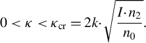
Here, I is the peak intensity, k is the absolute value of the wave vector in the medium, n ₀ is the unperturbed index of refraction and n ₂ is the effective cubic nonlinearity.

An important aspect of Equation (3) is that the boundaries of the instability band do not depend on the thickness of the nonlinear medium but are proportional to the square root of the peak intensity. As the peak intensity grows, increasingly more spatial frequencies are amplified due to cubic nonlinearity. At the same time, higher spatial frequencies are much easier to filter out. For laser radiation with λ = 910 nm and a peak intensity of 1 TW/cm², the characteristic angular (θ = κ/k) scale most susceptible to amplification inside the nonlinear sample is approximately 26 mrad for fused silica (n ₂ = 2.4×10^–7 cm²/GW). For such angles, free-space propagation significantly reduces the amplitudes of hazardous harmonics at the nonlinear medium input. The compressor is placed before the stage of additional compression (Figure 1). Since the beam in the compressor is propagating in free space over a considerable distance, at the nonlinear sample input, high spatial harmonics will lag in time behind the field component with κ_x = 0, κ_y = 0 and, besides, will escape from the strong-field region in the transverse direction. This will reduce their amplitude inside the nonlinear plate and, as a result, the nonuniformity of the transverse intensity distribution at the output of the nonlinear sample will be less compared to the case without filtering. Let us estimate this effect quantitatively.

4 Parameters for numerical simulation and controlled quantities

For numerical simulation, we choose a laser pulse with a central wavelength of 910 nm, a peak intensity of 0.5 TW/cm² and a half-maximum pulse duration of 50 fs. These parameters are close to the parameters of the beam at the output of the PEARL laser^[ Reference Mukhin, Glushkov, Soloviev, Shaykin, Ginzburg, Kuzmin, Martyanov, Stukachev, Mironov, Yakovlev and Khazanov ^{20 ]}. We assume that spectral broadening occurs in a 3-mm thick plane-parallel plate of fused silica, which corresponds to the B-integral of approximately 10 rad. In the approximation of plane monochromatic waves, for the specified parameters the right-hand boundary of the instability band in the nonlinear medium is κ _cr/k = 18.4 mrad. Taking into account the Snell refraction law, the angular interval [–θ _max, θ _max], where θ _max = κ _cr/k n ₀ = 26.7 mrad, is interesting for the analysis of spatial filtering. The value of κ _max should be chosen no less than the value of θ _max⋅k ₀. In turn, the choice of the maximum spatial frequency determines the characteristic spatial scale Λ = 2π/κ _max, to which this frequency corresponds. The choice of the size of the considered space [–X _max, X _max] and [–Y _max, Y _max] in the transverse x, y coordinates is determined by the need to exclude the influence of its boundaries on the field after the optical compressor. In other words, the effects leading to distortions of the transverse structure (e.g., diffraction) and linear displacement of the beam (e.g., with compressor asymmetry) should be localized within the considered area in the transversal space and not beyond its boundaries. At the same time, the number of points for field discretization along the x and y coordinates should be more than 2⋅(2⋅X _max/Λ) and 2⋅(2⋅Y _max/Λ).

The transverse intensity distribution of a regular field was chosen in the form of a super-Gaussian function (typical for high-power lasers) with diameter D and exponent N. The diffraction at the compressor output gives rise to rings in the transverse intensity distribution. The larger the value of D, the less the diffraction impact on the transverse profile. Larger N values correspond to sharper beam boundaries and, hence, stronger diffraction. Consequently, D and N should be chosen such that the diffraction should not significantly affect the transverse field structure after the compressor.

Of particular interest in the considered problem are the fluence fluctuations from the mean value of FL(x,y) and the squared absolute value of the spatial spectrum of FFL(κ_x , κ_y ). The FL(x,y) value is determined by $\mathrm{FL}\left(x,y\right)= \mathrm{NF}\left(x,y\right)- \mathrm{AV}$ , where $\mathrm{NF}\left(x,y\right)={\int}_{-\infty}^{\infty }I\left(x,y,t\right) \mathrm{d}t$ is the laser beam near field, and $\mathrm{AV}=\frac{1}{\varOmega }{\iint}_{\varOmega } \mathrm{NF}\left(x,y\right) \mathrm{d}x\mathrm{d}y$ is the mean value of intensity in the studied region of the beam Ω. Making use of the introduced notation, we can write an expression for the spectral density fluence fluctuation from the mean value of FFL(κ_x , κ_y ): $\mathrm{FFL}\left({\kappa}_x,{\kappa}_y\right)={\left|{\overset{\wedge }{F}}_{x,y}\left(\mathrm{FL}\left(x,y\right)\right)\right|}^2$ 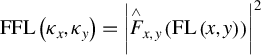, where ${\overset{\wedge }{F}}_{x,y}$ is a two-dimensional Fourier transform operator.

Note that the considered interval in time and its discretization are not arbitrary parameters either. When simulating a compressor and/or free space, a time delay of the spatial harmonics relative to the harmonics at the central frequency (κ_x = 0, κ_y = 0) is observed. A larger angle corresponds to a larger time delay. It is important to ensure that this time delay after passing the optical compressor should be within the chosen time interval. Note that we will consider the case when the pulse duration after the compressor is significantly less than the time delay introduced by the compressor with a symmetrical grating configuration for spatial harmonics that are well amplified in a medium with cubic nonlinearity. Also, we will consider the situation when the amplitude and energy of harmonic disturbances are small compared to the regular signal. For this, we will choose the parameter K equal to 10^–2.

5 Results of numerical simulation

We will start our consideration with a reference case: a nonlinear problem without a compressor, that is, the laser field (1) is forwarded into a nonlinear plate made of fused silica. The pulse characteristics (see Equation (1)) used as the initial condition at the boundary of the nonlinear sample are presented in experiments on extreme light–matter interaction (Figure 2). The field propagation in a nonlinear medium was simulated using the unidirectional pulse propagation equation taking into account cubic nonlinearity^[ Reference Couairon, Brambilla, Corti, Majus, de J. Ramírez-Góngora and Kolesik ^{21 ]}. Cubic nonlinearity leads to an increase in the amplitudes of the harmonics whose spatial frequencies lie in the instability band (3). According to the model of plane monochromatic waves, the maximum increase in amplitude occurs for the angular components ${\theta}_{\mathrm{max}\_ \mathrm{th}}=\sqrt{\frac{2\cdotp I\cdotp {n}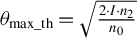_2}{n_0}}$ , and the right-hand boundary of the instability band is ${\theta}_{\mathrm{cr}}=2\cdotp \sqrt{\frac{I\cdotp {n}_2}{n_0}}$ 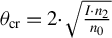. For the used parameters, ${\theta}_{\mathrm{max}\_ \mathrm{th}}$ = 13 mrad and θ _cr = 18 mrad inside the nonlinear sample. The values recalculated for vacuum are 18.9 and 26.13 mrad, respectively. Further, the angular diagrams from the nonlinear sample output are also recalculated for vacuum.

Figure 2

(а) Near-field. (b) Near-field cross-sections of the beam center along the x- and y-axes. (c) Two-dimensional distribution of fluence fluctuation from mean value of FL(x,y). (d) FL(x,y) cross-sections of the beam center along the x- and y-axes. (e) FFL(κ_x , κ_y ) distribution. (f)–(j) Similar field distributions at the output boundary of the nonlinear sample. The circles in Figures 2(a)) and 2(f) limit the analyzed fluence region; the circle in Figure 2(j) corresponds to $\theta$ ₁ ~ 16 mrad, at which gain is maximal.

Figure 2 Long description

The layout contains two rows of five panels each. Top row, from left: Panel a is a color heatmap with axes labeled in centimeters, showing a circular beam profile with a dashed circle and a colorbar from blue to red, values 0 to 25. Panel b is a line graph with x and y axes in centimeters and milliJoules per square centimeter, showing two overlaid traces labeled x-cross and y-cross, both flat-topped. Panel c is a color heatmap with axes in centimeters, showing a mostly uniform green field with small fluctuations, colorbar from -0.4 to 0.4. Panel d is a line graph with axes as in b, showing noisy traces for x-cross and y-cross centered around zero. Panel e is a color heatmap with axes in milliradians, showing a uniform blue field with small random yellow spots, colorbar from 0.01 to 0.05. Bottom row, from left: Panel f is a color heatmap with axes in centimeters, showing a ring-shaped profile with a dashed circle, colorbar from 0 to 140. Panel g is a line graph with axes as in b, showing noisy x-cross and y-cross traces with high peaks. Panel h is a color heatmap with axes in centimeters, showing a mostly blue field with sparse yellow spots, colorbar from 0 to 100. Panel i is a line graph with axes as in b, showing noisy x-cross and y-cross traces with high peaks. Panel j is a color heatmap with axes in milliradians, showing a ring-shaped pattern with a dashed circle, colorbar from 0 to 50000. The dashed circles in panels a, f, and j indicate the analyzed fluence region, with panel j corresponding to 1 to approximately 16 milliradians where gain is maximal.

According to the results of the numerical simulation (see Figure 2(j)), the maximum amplitude gain inside the nonlinear plate was achieved for the angular components (recalculated for vacuum) with ${\theta}_{\mathrm{max}\_ \mathrm{nm}}$ = 16 mrad, which is close to the value obtained using the plane monochromatic wave model. The value of ${\theta}_{\mathrm{max}\_ \mathrm{nm}}$ was determined by searching for the maximum of the FFL(κ_x , κ_y ) function (Figure 2(j)) averaged over the azimuthal angle. The ring thickness at the half level was 7 mrad. Note that the theoretical value lies within the ring’s width obtained numerically. The difference between the results of the numerical simulation and the theoretical estimate (16 versus 18.9 mrad) is explained by the fact that the amplification of harmonic disturbances occurs in a significantly saturated mode, where the considered theoretical model is not applicable. With the considered parameters of the problem, the value of the B-integral (here and below $B=\frac{2\pi }{\lambda}\cdot {n}_2\cdot {I}_\mathrm{peak}\left(z=0\right)\cdot L$ ) was approximately 10.2 rad, the modulation amplitude in the near-field increased by a factor of about 333 (cf. Figures 2(d) and 2(i)) and the intensity in the hot spots (filaments) exceeded the input intensity by several times. Such a beam is practically useless for further use. Note also that under the action of cubic nonlinearity a ring structure was formed in the spatial spectrum of the FL(x,y) function (cf. Figures 2(e) and 2(j)). The amplitude of the spatial harmonics, whose frequencies are in the instability band, increased from 0.05 to 5000 relative units, which resulted in an increase in the energy density modulation in the near-field.

Next, we consider the compressor influence. We consider a four-grating Treacy compressor with pairwise parallel gratings^[ Reference Treacy ^{22 ]}. As an example, we assume that the groove density is 1200 pcs/mm and the angle of incidence of the laser beam on the first grating is 45.5 degrees. For a symmetric compressor configuration, the distance between the gratings is d = 185 cm. For an asymmetric configuration, the distance between the gratings in the first and second pairs is smaller and larger by the value Δ, respectively, compared to the symmetric configuration. The distance between the grating pairs is assumed to be zero. This approximation is chosen solely because of the limited available computing resources and is aimed to reduce diffraction effects. Allowance for the distance between the gratings results in even stronger filtering of spatial harmonics. Figure 3 shows oscillograms of the pulses propagating at an angle to the z-axis before the compressor (Figure 3(a)), after the symmetric compressor (Figure 3(b)) and after the compressor with an asymmetric grating configuration (Figures 3(c) and 3(d)). The compressor causes the time delay of spatial harmonics with respect to the spatial frequency with a zero transverse wave vector. In the case of the symmetric compressor configuration, spatial harmonics with the same absolute value of the transverse wave vector, propagating in the groove plane and orthogonal to it, experience an identical time delay (Figure 3(b)). In this case, the time delay depends on the absolute value of the transverse component of the wave vector, but not on its direction. The compressor with a symmetric grating configuration works like free space. In the case of an asymmetric grating configuration, the situation is different. In the plane parallel to the grating grooves (YZ), the time delay τ ₁ with respect to the central frequency harmonic coincides with the case of the symmetric compressor. In the plane perpendicular to the grating grooves (XZ), the time delay has two values: larger than τ ₁ and smaller than τ ₁ (Figures 3(с) and 3(d)). The stronger the compressor asymmetry (the larger the Δ), the stronger the effect. Thus, for the asymmetric compressor, the time delay depends both on the absolute value of the transverse wave vector and on its orientation with respect to the direction of the diffraction-grating grooves. For certain spatial frequencies (as shown in Figure 3(d)), the spatial harmonics can overtake the harmonic with a zero spatial frequency. This occurs because the path of the harmonics is smaller than for the central spatial frequency. Also, there is a situation in which harmonics with non-zero spatial frequencies arrive at the end of the compressor simultaneously in time with a harmonic whose spatial frequency is zero. The situation will be discussed further.

Figure 3

Oscillograms of pulses propagating at an angle to the compressor axis: (a) before the compressor; (b) after the compressor with a symmetric grating configuration; (c), (d) with the asymmetric grating configuration Δ = ±5 cm and Δ = ±10 cm.

Figure 3 Long description

From left to right, panel a shows three overlapping curves with a symmetric, bell-shaped profile centered at zero on a linear-log scale, labeled by phi sub 0 and z values. Panel b displays the same parameter set after compression with a symmetric grating, where all curves exhibit sharp peaks near zero and diverge at higher times, with the blue curve peaking highest. Panels c and d show the results for asymmetric grating configurations with delta z equals plus or minus 5 centimeters and plus or minus 10 centimeters, respectively. In both, the blue curve remains highest and centered at zero, while the other curves shift rightward, forming distinct peaks at increasing time values as delta z increases. Legends in each panel specify phi sub 0 and z values for each curve. All axes are labeled Time, p s.

The time delay of the spatial harmonics with respect to the central frequency can be found from the following expression:

(4) $$\begin{align}\tau =\tau \left(\pm \boldsymbol{\kappa} \right)=\frac{{L}_\mathrm{f}{\kappa}^2}{2{k}_0{\omega}_0}+\frac{1}{2}{\psi}_{x x\omega}^{\prime \prime \prime }{k}_x^2+\frac{1}{2}{\psi}_{yy\omega}^{\prime \prime \prime }{k}_y^2\pm {\psi}_{x\omega}^{\prime \prime }{k}_x.\end{align}$$

Here, L _f is the distance between the input and output planes of the compressor (see Figure 1), ω is the laser frequency and ψ is the spectral phase introduced by the optical compressor^[ Reference Khazanov ^{16 ]}. In the case under study, L _f = 0. The input and output planes of the optical compressor can be selected differently. Obviously, the minimum distance (not a beam trace) between these planes is achieved when the input plane passes through the first compressor grating and the output plane passes through the last (fourth) one. In this case, the distance L _f can be significantly smaller compared to the distance between the gratings L. In this case, the contribution of free space to noise filtering and diffraction effects will be less compared to the contribution of the compressor itself. The approximation used is justified and can be used to investigate the effect of the compressor on noise filtering.

The values of the time delay found from Equation (4) coincide with the results of numerical simulation.

Next, we will consider the compressor impact on fluence fluctuations from the mean value before and after the nonlinear plate. The results of numerical simulation of laser beam propagation through the symmetric compressor are presented in Figures 4(a)–4(e) and at the output boundary of the nonlinear sample in Figures 4(f)–4(j).

Figure 4

Field parameters after the symmetric compressor: (a) near-field; (b) cross-sections of the beam center along the x and y coordinates; (c) two-dimensional distribution of fluence fluctuation from the mean value of FL(x,y); (d) FL(x,y) cross-sections along the x- and y-axes; (e) decimal logarithm of FFL(κ_x , κ_y ) after the compressor with the symmetric grating configuration; (f)–(j) similar distributions for the field at the output boundary of the nonlinear sample. The ring with the white dashed line in (a) and (f) limits the analyzed fluence area.

Figure 4 Long description

Top row, panels a to e: Panel a shows a color heatmap of a circular near-field fluence profile with concentric rings, axes labeled in centimeters, and a colorbar from 0 to 30. A white dashed ring marks the analysis area. Panel b presents two overlaid line plots labeled x-cross and y-cross, showing fluence versus position in centimeters, with both curves peaking at the edges and oscillating near the center. Panel c displays a two-dimensional color map of fluence fluctuation from the mean, with concentric contours and a colorbar from -2 to 2. Panel d shows cross-sections of these fluctuations along x and y, with oscillatory behavior centered at zero. Panel e is a two-dimensional color plot of the decimal logarithm of F F L kappa x, kappa y, axes in milliradians from -20 to 20, with a colorbar from -4 to 3, showing a central peak and radiating features. Bottom row, panels f to j: Panel f repeats the near-field fluence map after the nonlinear sample, with similar concentric structure and a white dashed ring. Panel g shows the corresponding x-cross and y-cross line plots, with slightly higher peak values. Panel h presents the two-dimensional fluence fluctuation map after the sample, with similar but subtly altered contours. Panel i shows the cross-sections of these fluctuations, maintaining oscillatory patterns. Panel j displays the logarithmic field distribution after the sample, with a central peak and radiating features, similar to panel e. All panels use consistent axis labels and colorbars for direct comparison.

The propagation through a compressor results in the formation of diffraction rings in the near-field and in a reduced amplitude modulation in the central part of the beam. The diffraction effects may be reduced by increasing the beam diameter. In the considered example this cannot be done in view of limited computational resources. Therefore, we analyzed fluence fluctuations from the mean value in the central part of the beam (the ring region in Figures 4(a) and 4(f)), where the impact of diffraction is minimal.

After the symmetric compressor, the modulation amplitude in the central part of the beam decreases by approximately 10 times relative to the initial field distribution. The spatial noise is almost filtered by the symmetric compressor. We attribute the remaining modulation in the laser beam to the diffraction effect. The nonlinear medium slightly changes the field distribution at the output of the nonlinear plate. The amplitude of harmonic disturbances remains virtually unchanged after passing the nonlinear plate. The key reason is the time mismatch between the well-amplified harmonics and the harmonic at zero spatial frequency, that is, the wave from which the energy flows due to self-focusing instability.

It should be noted that spatial noise can be observed in experiments conducted at a real laser facility. There are no contradictions with the presented results. The following facts can be used to explain the phenomenon. Firstly, in our numerical simulations, we do not consider the quality of the compressor gratings, which can be a source of spatial noise. Secondly, spatial noise in a laser beam can appear on any surface of the optical elements (mirrors, lenses, neutral filters, etc.) used in the beam line placed after the grating compressor and in a diagnostic setup.

Let us consider the effect of compressor asymmetry on the noise level after the nonlinear plate. Compressor asymmetry leads to the formation of the spectrum structure of the FFL(κ_x , κ_y ) function, consisting of two rings touching at the point (κ_x = 0, κ_y = 0). This effect has a simple physical explanation. Equation (4) for the time delay transforms to the following:

(5) $$\begin{align}\tau \left(\boldsymbol{\kappa} \right)&=\left(\frac{{L}_\mathrm{f}}{2{k}_0{\omega}_0}+\frac{1}{2}{\psi}_{x x\omega}^{\prime \prime \prime}\right)\cdot {\left({k}_x\pm \frac{\psi_{x\omega}^{\prime \prime }}{2\cdot \left(\frac{{L}_\mathrm{f}}{2{k}_0{\omega}_0}+\frac{1}{2}{\psi}_{x x\omega}^{\prime \prime \prime}\right)}\right)}^2\nonumber\\&\quad+\left(\frac{{L}_\mathrm{f}}{2{k}_0{\omega}_0}+\frac{1}{2}{\psi}_{yy\omega}^{\prime \prime \prime}\right)\cdot {k}_y^2-\frac{{\psi_{x\omega}^{\prime \prime}}^2}{4\cdot \left(\frac{{L}_\mathrm{f}}{2{k}_0{\omega}_0}+\frac{1}{2}{\psi}_{x x\omega}^{\prime \prime \prime}\right)}.\end{align}$$

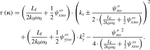
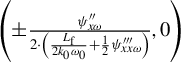
The set of values of the transverse wave vectors κ, for which the time delay is $\tau \left(\boldsymbol{\kappa} \right)=0,$ is just a line consisting of two touching rings. The ring centers are located at the points $\left(\pm \frac{\psi_{x\omega}^{\prime \prime }}{2\cdot \left(\frac{{L}_\mathrm{f}}{2{k}_0{\omega}_0}+\frac{1}{2}{\psi}_{x x\omega}^{\prime \prime \prime}\right)}, 0\right)$ , and their radius is $R=\frac{\psi_{x\omega}^{\prime \prime }}{2\cdot \left(\frac{{L}_\mathrm{f}}{2{k}_0{\omega}_0}+\frac{1}{2}{\psi}_{x x\omega}^{\prime \prime \prime}\right)}$ 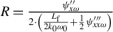. This line corresponds to the set of harmonics that arrive at the compressor output synchronously with the harmonic at zero spatial frequency and are not filtered in time.

For further analysis we will take three cases. (1) The compressor grating asymmetry is so small that the diameters of the formed rings of the FFL(κ_x , κ_y ) function are much smaller than ${\theta}_{\mathrm{max}\_ \mathrm{nm}}$ . Obviously, in this case, the noise level after the nonlinear plate will be equal to or slightly higher than in a compressor with symmetric grating configuration if it is placed in front of the plate. (2) The second case corresponds to the situation when the rings of the FFL(κ_x , κ_y ) function touch the ring of radius θ = θ _{max_nm} . An example of such an option is shown in Figure 5(e). With the parameters under consideration, such a case is realized for an asymmetry of the distances between the gratings Δ = 5 cm. Note that for the studied compressor, the calculated ring radius R/k ₀ = 8.3 mrad agrees well with Figures 5(е) and 5(j). In Figure 5(j), the ring diameter is θ = 15 mrad, that is, each ring touches the ring θ = ${\theta}_{\mathrm{max}\_ \mathrm{nm}}$ (taking into account its width) at one point: (θ_x = ${\theta}_{\mathrm{max}\_\mathrm{nm}}$ , θ_y = 0) and (θ_x = – ${\theta}_{\mathrm{max}\_\mathrm{nm}}$ , θ_y = 0). In Figure 5(j), the areas where the rings touch have a higher intensity. This is due to the amplification in the medium with cubic nonlinearity. (3) The compressor asymmetry is so large that the rings of the FFL(κ_x , κ_y ) function intersect the ring with radius θ = θ _{max_nm}. This case is illustrated in Figure 6, which corresponds to the asymmetry of the distances between the gratings Δ = 10 cm. In the area of ring intersection, the amplitudes of the corresponding harmonics increase (see Figure 6(j)).

Figure 5

Field parameters after an asymmetric compressor (Δ = 5 cm): (a) near-field; (b) near-field cross-sections of the beam center along the x and y coordinates; (c) two-dimensional distribution of fluence fluctuation from the mean value of FL(x,y); (d) FL(x,y) cross-sections along the x- and y-axes; (e) decimal logarithm of FFL(κ_x , κ_y ); (f)–(j) similar distributions for the field at the output boundary of the nonlinear medium. The rings in (a) and (f) limit the analyzed fluence area; the small rings in (e) and (j) correspond to spatial frequencies propagating synchronously with the harmonic at zero spatial frequency, while the large rings correspond to maximum gain of the spatial harmonics in a medium with cubic nonlinearity.

Figure 5 Long description

Top row panels a to e show near-field analysis after an asymmetric compressor with delta equals 5 centimeters. Panel a is a color heatmap of fluence in the x-y plane, centered at zero, with a dashed ring marking the analyzed area and a colorbar from 0 to 30 millijoules per square centimeter. Panel b presents two line plots, labeled x-cross and y-cross, showing fluence cross-sections along x and y axes, with peaks near the ring boundaries. Panel c is a two-dimensional color map of fluence fluctuation from the mean, with a colorbar from minus 2.5 to plus 2.5. Panel d shows line plots of these fluctuations along x and y axes, with oscillatory features. Panel e is a two-dimensional map in spatial frequency space, axes labeled in milliradians, showing the decimal logarithm of F F L kappa x, kappa y, with small and large dashed rings indicating synchronous and maximum gain spatial frequencies, colorbar from minus 4 to plus 3. Bottom row panels f to j repeat the analysis for the field at the output boundary of the nonlinear medium. Panel f is a fluence heatmap with a dashed ring, colorbar from 0 to 50. Panel g shows x and y cross-sections with higher and flatter central values. Panel h is a fluctuation map with a colorbar from minus 6 to plus 6. Panel i shows more pronounced oscillations in the cross-sections. Panel j is a frequency domain map with similar ring annotations, colorbar from minus 4 to plus 3. All axes and colorbars are labeled, and the rings in panels a, e, f, and j denote regions of interest in real and frequency space.

Figure 6

Field parameters after the asymmetric compressor (Δ = 10 cm): (a) near-field; (b) sections passing through the beam center along the x and y coordinates; (c) two-dimensional distribution of fluence fluctuation from the mean value of FL(x,y); (d) decimal logarithm of FFL(κ_x , κ_y ); (e) decimal logarithm of FFL(κ_x , κ_y ) after the compressor with the asymmetric grating configuration; (f)–(j) similar distributions for the field at the output boundary of the nonlinear medium. The rings in (a) and (f) limit the analyzed fluence region, while the small rings in (e) and (j) correspond to spatial frequencies propagating synchronously with the harmonic at zero spatial frequency and the large rings correspond to maximum gain of the spatial harmonics in a medium with cubic nonlinearity.

Figure 6 Long description

Top row, from left to right: Panel a shows a color heatmap of fluence in the near-field, with a dashed ring marking the analysis region, axes labeled in centimeters, and a colorbar from 5 to 30. Panel b is a line graph with x and y axes in centimeters and millijoules per square centimeter, plotting x-cross and y-cross fluence profiles with a plateau and edge peaks. Panel c is a color heatmap of fluence fluctuation from the mean, with a central blue region and red edges, axes in centimeters, colorbar from -4.5 to 4.5. Panel d is a line graph of fluence fluctuation cross-sections, showing oscillations around zero, axes as above. Panel e is a two-dimensional map in milliradians of the decimal logarithm of fluence fluctuation in spatial frequency space, with a dashed ring at the center and a colorbar from -3 to 3. Bottom row, left to right: Panel f repeats the fluence heatmap for the output field, with a dashed ring and colorbar from 5 to 35. Panel g is a line graph of x-cross and y-cross fluence at output, showing a broader plateau and sharper edges. Panel h is a heatmap of output fluence fluctuation, with a central blue region and red edges, colorbar from -3 to 3. Panel i is a line graph of output fluence fluctuation cross-sections, showing increased noise and oscillations. Panel j is a two-dimensional map of the decimal logarithm of output fluence fluctuation in spatial frequency space, with small and large dashed rings indicating synchronously propagating and maximum gain spatial frequencies. All panels include precise axis labels and colorbars.

With an asymmetric compressor configuration, the filtering of spatial harmonics propagating in the plane orthogonal to the diffraction-grating grooves is more efficient. The resulting amplitude of the rings acquired by the beam due to diffraction in this plane decreases compared to the orthogonal one (cf. the cuts in the x and y planes in Figures 5(b) and 6(b)). The distribution of the FL(x,y) function also differs from the symmetric compressor configuration (cf. Figures 4(с) and 4(d) with Figures 5(с), 5(d), 6(с) and 6(d)). The inhomogeneities in the plane transverse to the grooves smooth out. These factors have a positive effect on the modulation level of the near-field at the compressor output.

For the second and third cases, the modulation of the FL(x,y) function at the output of the nonlinear plate is slightly higher than in the case of a compressor with symmetric grating configuration located in front of the nonlinear plate. The point is that with the asymmetric compressor grating configuration, spatial harmonics subject to amplification are preserved in the beam. This occurs either when the FFL(κ_x , κ_y ) function touches the ring of radius θ = θ _{max_nm} or when they intersect. The compressor with the asymmetric grating configuration does not fully filter the components subject to amplification. Moreover, some of them propagate synchronously in time with a strong wave for which κ_x = 0, κ_y = 0 (Figures 5(c), 5(d), 6(c) and 6(d)). Despite the fact that with the use of an asymmetric compressor near-field inhomogeneities are smoothed out in the plane orthogonal to the grating grooves, harmonic disturbances in a nonlinear medium are amplified more effectively than in the case of a symmetric compressor or a compressor with a small asymmetry in the grating arrangement.

The results of the numerical simulations are summarized in Table 1, which presents the RMS (root mean square) and PV (peak-to-valley) parameters of the FL(x, y) functions for the considered cases. According to the table, the smallest PV parameter after the nonlinear plate can be obtained by using a grating compressor with a symmetric grating configuration. As far as the PV parameter reflects the possibility of destroying optical elements (the smaller the parameter, the lower the probability), it is important to choose a configuration of optical compressor to minimize it. Thus, a symmetric compressor is preferable for filtering spatial noise.

Table 1

Fluence characteristics before and after the compressors.

Table 1 Long description

From left to right, the first column lists R M S and P V in millijoules. The next two columns show initial values: R M S is 0.10, P V is 0.98; after the plate, R M S is 21.05, P V is 154.03. For Delta equals 0 centimeters, compressor R M S is 0.91, plate R M S is 0.97; compressor P V is 4.89, plate P V is 5.12. For Delta equals 5 centimeters, compressor R M S is 0.42, plate R M S is 0.88; compressor P V is 4.38, plate P V is 10.30. For Delta equals 10 centimeters, compressor R M S is 0.30, plate R M S is 0.52; compressor P V is 2.61, plate P V is 5.53.

From the perspective of spatial effects, the compressor with the symmetric grating configuration is similar to free space, but it introduces astigmatism, as the x- and y-directions are no longer equivalent. Thus, the compressor is equivalent to free space with different lengths on the x- and y-axes^[ Reference Khazanov ^{16 ]}. The time delay between spatial harmonics and the harmonic with zero spatial frequency depends on the distance between the grating pairs, but for the Treacy compressor, all non-zero spatial frequencies are delayed in time, and none can arrive faster or at the same time as the zero frequency even in the case where the distance between the grating pairs is not equal to zero. This is not the case for a compressor with an asymmetric grating configuration. For such a compressor, there is always a set of spatial frequencies that arrive simultaneously in time with the zero frequency. Moreover, some noise spatial harmonics may precede the main pulse, resulting in deterioration of temporal contrast. Thus, the spatial harmonics synchronous with the main pulse will interact in the nonlinear sample with a strong spatial harmonic at zero frequency, which will lead to an effective amplification process. This means that after the Treacy compressor, the interaction inside the nonlinear sample between zero and non-zero harmonics will always be worse compared to the cases with no compressor and with a compressor having an asymmetric grating configuration. The reason for this is based on poorer temporal overlap.

A compressor consisting of two gratings deserves special consideration^[ Reference Trentelman, Ross and Danson ^{23 ,} Reference Vyatkin and Khazanov ^{24 ]}. Formally, it is a particular case of an asymmetric compressor with a very large asymmetry parameter Δ equal to the distance between the gratings. In this case, the rings touching each other at the point (0,0) transform into vertical lines k_x = 0. This can qualitatively improve the suppression of SSSF, but significantly more computing resources are needed for simulation, which is beyond the scope of this work.