2.1. Mathematical model

We consider an incompressible, body-forced, stably stratified flow with streamwise velocity field aligned with the $x$-axis. In accordance with the Spiegel–Veronis–Boussinesq approximation (Spiegel & Veronis Reference Spiegel and Veronis1960), we assume that the basic state comprises a linearised temperature distribution $T_b(z)$ given by $T_b(z)=T_0 + z (\textrm {d} T_b / \textrm {d} z)$, where $T_0$ is a reference temperature, along with a body-forced laminar velocity field $\boldsymbol {u}_L(y)$. The total temperature field, $T$, includes perturbations $T'(x,y,z,t)$ away from the basic state such that $T = T_b(z) + T'(x,y,z,t)$. As discussed in § 1.2, the density fluctuations $\rho '$ and temperature fluctuations $T'$ are related according to the linearised equation of state

(2.1)\begin{equation} \frac{\rho'}{\rho_0}= - \alpha T', \end{equation}

where $\rho _0$ is a reference density and $\alpha =- \rho _0^{-1} (\partial \rho / \partial T)$ is the coefficient of thermal expansion. The three-dimensional velocity field is given by $\boldsymbol {u}(x,y,z,t) = u \boldsymbol {e}_x + v \boldsymbol {e}_y + w \boldsymbol {e}_z$. For numerical efficiency, we impose triply periodic boundary conditions on the body force $\boldsymbol {F}$ and the variables $T'$ and $\boldsymbol {u}$ such that $(x,y,z) \in [0,L_x) \times [0,L_y) \times [0,L_z)$. A suitable candidate for the applied force is a monochromatic sinusoidal forcing driving a horizontal Kolmogorov flow

(2.2)\begin{equation} \boldsymbol{F} \propto \sin \left ( \frac{2{\rm \pi} y}{L_y} \right) \boldsymbol{e}_x. \end{equation}

This choice of forcing is computationally straightforward to implement and was selected following the work of Lucas et al. (Reference Lucas, Caulfield and Kerswell2017) who studied horizontally sheared stratified flows at $Pr = 1$. 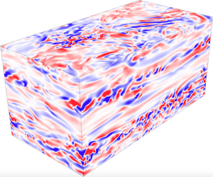The monochromatic Kolmogorov forcing was also used by Balmforth & Young (Reference Balmforth and Young2002) to study vertically sheared stratified flows at high $Pr$, and by Garaud, Gallet & Bischoff (Reference Garaud, Gallet and Bischoff2015a) and Garaud & Kulenthirarajah (Reference Garaud and Kulenthirarajah2016) for vertically sheared stratified flows at low $Pr$ (and in the low $Pe$ limit). It has the advantage of being linearly unstable (as shown below), in contrast with other set-ups such as the shearing box that only have finite amplitude instabilities. Figure 1 illustrates the basic laminar state.

Figure 1. Schematics of the basic state set-up showing (a) the linearised background temperature distribution $T_b(z)$ and (b) the laminar body-forced velocity profile $\boldsymbol {u}_L(y)$.

The governing Spiegel–Veronis–Boussinesq equations (Spiegel & Veronis Reference Spiegel and Veronis1960) for this model set-up are

(2.3)\begin{gather} \frac{\partial \boldsymbol{u}}{\partial t} + \boldsymbol{u} \boldsymbol{\cdot} \boldsymbol{\nabla} \boldsymbol{u} + \frac{1}{\rho_0} \boldsymbol{\nabla} p = \nu \nabla^2 \boldsymbol{u} + \alpha g T' \boldsymbol{e}_z + \chi \sin \left( \frac{2{\rm \pi} y}{L_y} \right) \boldsymbol{e}_x, \end{gather}

(2.4)\begin{gather}\frac{\partial T'}{\partial t} + \boldsymbol{u} \boldsymbol{\cdot} \boldsymbol{\nabla} T' + w \left ( \frac{\textrm{d} T_b}{\textrm{d} z} + \frac{g}{c_p} \right ) = \kappa \nabla^2 T', \end{gather}

(2.5)\begin{gather}\boldsymbol{\nabla} \boldsymbol{\cdot} \boldsymbol{u} = 0, \end{gather}

where $\nu$ is the kinematic viscosity, $\kappa$ is the thermal diffusivity, $\chi$ is the forcing amplitude, $p$ is the pressure, $c_p$ is the specific heat at constant pressure and gravity $g$ acts in the negative $z$-direction. In this study, we specify that $L_y = L_z$ while $L_x$ may vary continuously such that the aspect ratio of the domain is given by $\lambda = L_x / L_y$. The case $\lambda > 1$ corresponds to domains which are longer in the streamwise direction.

2.2. Non-dimensionalisation and model parameters

In equilibrium, we anticipate a balance between the body force and fluid inertia such that $\boldsymbol {u} \boldsymbol {\cdot } \boldsymbol {\nabla } \boldsymbol {u} \sim \chi \sin ( 2{\rm \pi} y/L_y ) \boldsymbol {e}_x$ in the streamwise direction. For a characteristic length scale $L_y/2{\rm \pi}$, this gives a characteristic velocity scale $\sqrt { \chi L_y / 2{\rm \pi} }$ and a characteristic time scale $\sqrt {L_y/2{\rm \pi} \chi }$. Combined with the vertical temperature gradient scale $(\textrm {d} T_b / \textrm {d} z + g/c_p)$, we use the equivalent non-dimensionalisation as in Lucas et al. (Reference Lucas, Caulfield and Kerswell2017) to give the following system of equations, in which all quantities are non-dimensional:

(2.6)\begin{gather} \frac{\partial \boldsymbol{u}}{\partial t} + \boldsymbol{u} \boldsymbol{\cdot} \boldsymbol{\nabla} \boldsymbol{u} + \boldsymbol{\nabla} p = \frac{1}{Re} \nabla^2 \boldsymbol{u} + B T' \boldsymbol{e}_z + \sin (y) \boldsymbol{e}_x, \end{gather}

(2.7)\begin{gather}\frac{\partial T'}{\partial t} + \boldsymbol{u} \boldsymbol{\cdot} \boldsymbol{\nabla} T' + w = \frac{1}{RePr} \nabla^2 T', \end{gather}

(2.8)\begin{gather}\boldsymbol{\nabla} \boldsymbol{\cdot} \boldsymbol{u} = 0. \end{gather}

We thus have three non-dimensional numbers: the Reynolds number $Re$; the buoyancy parameter $B$; and the Prandtl number $Pr$, which determine the dynamics of the system:

(2.9a–c)\begin{equation} Re := \frac{\sqrt{\chi}}{\nu} \left( \frac{L_y}{2{\rm \pi}} \right)^{{3}/{2}}, \quad B := \frac{\alpha g (\textrm{d} T_b / \textrm{d} z + g / c_p) L_y}{2{\rm \pi} \chi} = \frac{N_b^2 L_y}{2{\rm \pi} \chi}, \quad Pr := \frac{\nu}{\kappa}, \end{equation}

where $N_b$ is the dimensional buoyancy frequency defined in (1.10), which is now constant by construction. Note that $B$ is related to the Froude number as

(2.10)\begin{equation} B = Fr^{-2}. \end{equation}

It is also convenient to introduce the Péclet number $Pe$, defined as

(2.11)\begin{equation} Pe := Re Pr = \frac{\sqrt{\chi}}{\kappa}\left( \frac{L_y}{2{\rm \pi}} \right)^{{3}/{2}}.\end{equation}

Both sets of parameters, ($Re$, $B$, $Pr$) or ($Re$, $B$, $Pe$), uniquely define the system and will be used interchangeably throughout this study. In all that follows, the domain is a cuboid such that $(x,y,z) \in [0,{2{\rm \pi} \lambda }) \times [0,{2{\rm \pi} }) \times [0,{2{\rm \pi} })$, and variables $p$, $T'$ and $\boldsymbol {u}$ have triply periodic boundary conditions. This system, defined by (2.6)–(2.8), will henceforth be referred to as the standard system of equations.

2.3. Low Péclet number approximation

As discussed in § 1.2, when the thermal diffusion time scale is much shorter than the advective time scale, a quasi-static regime is established where temperature fluctuations are slaved to the vertical velocity field. Motivated by the astrophysical applications described in § 1.2, we consider the standard set of (2.6)–(2.8) in the asymptotic limit of low Péclet number (LPN). This limit was studied by Spiegel (Reference Spiegel1962) and Thual (Reference Thual1992) in the context of thermal convection, and more recently by Lignières (Reference Lignières1999) in the context of stably stratified flows. Lignières proposed that the standard equations can be approximated by a reduced set of equations called the ‘low Péclet number’ equations (LPN equations hereafter), in which the density fluctuations are slaved to the vertical velocity field:

(2.12)\begin{gather} \frac{\partial \boldsymbol{u}}{\partial t} + \boldsymbol{u} \boldsymbol{\cdot} \boldsymbol{\nabla} \boldsymbol{u} + \boldsymbol{\nabla} p = \frac{1}{Re} \nabla^2 \boldsymbol{u} + B T' \boldsymbol{e}_z + \sin (y) \boldsymbol{e}_x, \end{gather}

(2.13)\begin{gather}w - \frac{1}{Pe} \nabla^2 T' = 0, \end{gather}

(2.14)\begin{gather}\boldsymbol{\nabla} \boldsymbol{\cdot} \boldsymbol{u} = 0. \end{gather}

These can be derived by assuming a regular asymptotic expansion of $T'$ in powers of $Pe$, i.e. $T'=T'_0 + T'_1 Pe + O(Pe^2)$, and by assuming that the velocity field is of order unity. At lowest order ($Pe^{-1}$), we get $\nabla ^2 T'_0=0$ implying that $T'_0=0$ is required to satisfy the boundary conditions, while at the next order ($Pe^{0}$), the equations yield $w = \nabla ^2 T'_1 \approx Pe^{-1}\nabla ^2 T'$ as required.

Noting that (2.13) can be re-written formally as $T'=Pe \nabla ^{-2}w$, we derive the reduced set of LPN equations

(2.15)\begin{gather} \frac{\partial \boldsymbol{u}}{\partial t} + \boldsymbol{u} \boldsymbol{\cdot} \boldsymbol{\nabla} \boldsymbol{u} + \boldsymbol{\nabla} p = \frac{1}{Re} \nabla^2 \boldsymbol{u} + BPe \nabla^{-2}w \boldsymbol{e}_z + \sin (y) \boldsymbol{e}_x, \end{gather}

(2.16)\begin{gather}\boldsymbol{\nabla} \boldsymbol{\cdot} \boldsymbol{u} = 0. \end{gather}

These equations explicitly demonstrate that under the LPN approximation (and in contrast to the standard equations), there are only two non-dimensional parameters governing the flow dynamics, notably the Reynolds number $Re$ and the product of the buoyancy parameter and the Péclet number, $BPe = Pe Fr^{-2}$. This combined parameter, which we consider to be a measure of the stratification, can take any value (even for small Péclet numbers) because $B$ can be arbitrarily large, or equivalently $Fr$ can be arbitrarily small, as the stratification becomes strong.

There are advantages of studying the LPN equations rather than the standard equations. For example, this reduced set of equations allows for the derivation of mathematical results such as an energy stability threshold that explicitly depends on $BPe$ (see Garaud et al. Reference Garaud, Gallet and Bischoff2015a). Throughout this study, we will discuss both systems of equations, verifying the validity of the LPN equations where possible.

3.1. Standard equations

We begin by considering the stability of a laminar flow to infinitesimal perturbations, with initial focus on the standard set of (2.6)–(2.8). The background flow $\boldsymbol {u}_L(y)$, which satisfies $Re^{-1}\nabla ^2 \boldsymbol {u}_L + \sin (y) \boldsymbol {e}_x =0$, is given by

(3.1)\begin{equation} \boldsymbol{u}_L(y) = Re \sin (y) \boldsymbol{e}_x. \end{equation}

Note that if one wishes to consider a basic state with generic amplitude $aRe$ instead of amplitude $Re$, it is straightforward to apply a rescaling using the method described in appendix A. For small perturbations $\boldsymbol {u}'(x,y,z,t)$ away from this laminar flow, i.e. letting $\boldsymbol {u} = \boldsymbol {u}_L(y) + \boldsymbol {u}'(x,y,z,t)$, the linearised perturbation equations are

(3.2)\begin{gather} \frac{\partial \boldsymbol{u}'}{\partial t} + Re \cos (y) v' \boldsymbol{e}_x + Re \sin(y) \frac{\partial \boldsymbol{u}'}{\partial x} + \boldsymbol{\nabla} p = \frac{1}{Re} \nabla^2 \boldsymbol{u}' + BT' \boldsymbol{e}_z, \end{gather}

(3.3)\begin{gather}\frac{\partial T'}{\partial t} + Re \sin(y) \frac{\partial T'}{\partial x} + w' = \frac{1}{RePr} \nabla^2 T', \end{gather}

(3.4)\begin{gather}\boldsymbol{\nabla} \boldsymbol{\cdot} \boldsymbol{u}' = 0. \end{gather}

In this set of partial differential equations, the coefficients are periodic in $y$ but independent of $x$, $z$ and $t$. Consequently, and in the conventional fashion, we consider normal mode disturbances of the form

(3.5)\begin{equation} q(x,y,z,t) = \hat{q}(y) \exp[\textrm{i}k_x x + \textrm{i}k_z z + \sigma t], \end{equation}

where $q \in (u', v', w', T', p)$ and $k_x$ and $k_z$ are the perturbation wavenumbers in the $x$ and $z$-directions respectively. The geometry of the model set-up requires that $k_x \in \mathbb {R}$ and $k_z \in \mathbb {Z}$. We seek periodic solutions for $\hat {q}(y)$ given by

(3.6)\begin{equation} \hat{q}(y) = \sum_{l=-L}^{L} q_l \textrm{e}^{ily}. \end{equation}

Substituting this ansatz into (3.2)–(3.4) and using the orthogonality property of complex exponentials, we obtain a $5 \times (2L+1) = (10L+5)$ algebraic system of equations for the $u_l$, $v_l$, $w_l$, $T_l$ and $p_l$ for $l \in (-L,L)$:

(3.7)\begin{gather} \frac{1}{2}Re k_x (u_{l+1} -u_{l-1}) - \frac{l^2 + k_x^2 + k_z^2}{Re} u_l - \frac{1}{2}Re(v_{l-1} + v_{l+1}) - ik_x p_l = \sigma u_l, \end{gather}

(3.8)\begin{gather}\frac{1}{2}Re k_x (v_{l+1} -v_{l-1}) - \frac{l^2 + k_x^2 + k_z^2}{Re} v_l - il p_l = \sigma v_l, \end{gather}

(3.9)\begin{gather}\frac{1}{2}Re k_x (w_{l+1} -w_{l-1})- \frac{l^2 + k_x^2 + k_z^2}{Re} w_l + B T_l - ik_z p_l = \sigma w_l, \end{gather}

(3.10)\begin{gather}\frac{1}{2}Re k_x (T_{l+1} -T_{l-1}) - w_l - \frac{l^2 + k_x^2 + k_z^2}{RePr} T_l = \sigma T_l, \end{gather}

(3.11)\begin{gather}k_x u_l + lv_l + k_z w_l = 0. \end{gather}

This system can be re-formulated as a generalised eigenvalue problem for the complex growth rates $\sigma$,

(3.12)\begin{equation} \boldsymbol{A}(k_x,k_z,Re,B,Pr) \boldsymbol{X} = \sigma \boldsymbol{B}\boldsymbol{X}, \end{equation}

where $\boldsymbol {X} = (u_{-L},\ldots ,u_L,v_{-L},\ldots ,v_L,w_{-L},\ldots ,w_L,T_{-L},\ldots ,T_L,p_{-L},\ldots ,p_L)$, $\boldsymbol {A}$ and $\boldsymbol {B}$ are $(10L+5)\times (10L+5)$ square matrices and $\boldsymbol {B}_{i,j}= \{\delta _{ij}, i,j \leq (8L+4); 0, \textrm {otherwise}\}$. Equation (3.12) has $(10L+5)$ eigenvalues $\sigma$. For perturbation wavenumbers $k_x$ and $k_z$ and system parameters $Re$, $B$ and $Pr$, the eigenvalue with the largest real part determines the growth rate of the linear instability. The eigenvalue problem can be solved numerically, with $L$ chosen such that convergence is achieved.

3.1.1. Comparison with previous results at $Pr=1$

We first consider the case of $Pr=1$ for ease of comparison with previous work. Deloncle, Chomaz & Billant (Reference Deloncle, Chomaz and Billant2007), Arobone & Sarkar (Reference Arobone and Sarkar2012) and Park, Prat & Mathis (Reference Park, Prat and Mathis2020) each considered the linear stability of horizontal shear layers with somewhat different base flows, and Lucas et al. (Reference Lucas, Caulfield and Kerswell2017) considered the linear stability of the specific horizontally sheared Kolmogorov flow considered here, exclusively for $Pr=1$. Letting $B=100$, we consider the linear stability of the basic state flow $\boldsymbol {u}_L$ (see (3.1)) across a range of Reynolds numbers for both two-dimensional (2-D) and 3-D perturbation modes.

Figure 2(a) shows the neutral stability curves ($\sigma =0$) for varying vertical wavenumbers $k_z \in (0,\ldots ,6)$ in the $(Re,k_x)$ space. Our results are in agreement with those of Lucas et al. (Reference Lucas, Caulfield and Kerswell2017). Stability ($\sigma < 0$) is found to the left and above the curves whilst instability ($\sigma > 0$) occurs to the right and below. The black curve illustrates the 2-D ($k_z=0$) mode. This neutral stability curve intercepts the $x$-axis when $Re=2^{1/4}\simeq 1.19$, implying that the system is linearly stable when $Re<2^{1/4}$ (in agreement with Beaumont Reference Beaumont1981; Balmforth & Young Reference Balmforth and Young2002, once the correct rescaling is applied (see appendix B for details)). For large $Re$, it asymptotes to $k_x=1$ but, in agreement with Lucas et al. (Reference Lucas, Caulfield and Kerswell2017), always lies below this line, leading to the conclusion that domains such that $\lambda = L_x / L_y \leq 1$ are linearly stable to the 2-D mode.

Figure 2. (a) Neutral stability curves for a range of $k_z$ wavenumbers as a function of Reynolds number and $k_x$ wavenumber, with instability occurring to the right and below the curves. Variation with Reynolds number for a collection of $k_z$ wavenumbers of: (b) the largest growth rate $\sigma _{max}$ maximised across all horizontal wavenumbers $k_x$; (c) the associated horizontal wavenumber $k_{x,max}$. The curves plotted include $k_z=0$ (black) and $k_z =1, 2, 3, 4, 5, 6$ (coloured) and the standard equations were used with $B=100$ and $Pr=1$ fixed (so $Pe=Re$).

The coloured curves show the neutral stability curves for the first six 3-D modes ($k_z \in (1,\ldots ,6)$). The onset of instability in the 3-D modes is found to occur for higher Reynolds numbers than the 2-D mode, with the critical Reynolds number for instability of these 3-D modes increasing monotonically with increasing $k_z$. For a range of $Re \sim O(100)$ (corresponding to $Pe \sim O(100)$), the 3-D curves actually cross the line $k_x=1$ implying that these modes are unstable for domains where $\lambda =1$, i.e. cubic domains.

Figures 2(b) and 2(c) further analyse the information in figure 2(a) by computing, for each Reynolds number and $k_z$, the largest (positive) growth rate, $\sigma _{max}$, across all values of $k_x$ and the value of $k_x$ for which that maximum is achieved, $k_{x,max}$. We see that, as well as being the mode that becomes unstable first, the 2-D mode is always the fastest growing one. In addition, the ratio of the growth rate of the 2-D mode to that of the 3-D modes increases with $Re$. We therefore predict that the 2-D mode would strongly influence the dynamics when it is unstable (i.e. for domain sizes such that $\lambda >1$). Finally, we note that the corresponding streamwise wavenumbers of the fastest growing 3-D modes satisfy $k_{x,max} \to 0$ in the limit $Re \to \infty$, while those of the fastest growing 2-D mode remain constant.

3.1.2. Stability at low $Pr$

Astrophysical applications motivate an understanding of the effects of the stratification parameter $B$ and Prandtl number $Pr$ on the linear stability of the basic state. Consequently, in figure 3(a–c) we plot the neutral stability curves in exactly the same fashion as in figure 2(a), for three different Prandtl numbers: $Pr=0.1$ (first column), $Pr=0.01$ (second column) and $Pr=0.001$ (third column), keeping $B=100$ constant. Whilst the neutral stability curves for the 2-D mode are identical, clear trends exist for the 3-D modes. A reduction in the value of $Pr$ shifts the critical Reynolds numbers for the onset of instability of the 3-D modes towards higher values, thereby making these modes less unstable. This result is consistent with Arobone & Sarkar (Reference Arobone and Sarkar2012) and Park et al. (Reference Park, Prat and Mathis2020), who investigated the stability of a diffusive, stratified, horizontally sheared hyperbolic flow. We also note that the same trend is found by letting $B \to 0$ and keeping $Pr$ constant (not plotted). Thus, $B \to 0$ (at fixed $Pr$) and $Pr \to 0$ (at fixed $B$) have the same effect: the 3-D modes of instability are suppressed while the 2-D mode remains unstable. The explanation for this emerges from consideration of (2.7). As the Prandtl number tends to zero (keeping the Reynolds number finite), the Péclet number becomes small and so the buoyancy diffusion becomes important. In this case, a parcel of fluid that is advected into surrounding fluid of a different density adjusts very rapidly to its surroundings, thereby reducing the buoyancy force and so approximating an unstratified system.

Figure 3. A comparison of linear stability analysis results between the standard equations (top row) and the LPN equations (bottom row). Neutral stability curves for a range of $k_z$ wavenumbers ($k_z=0$ (black) and $k_z =1, 2, 3, 4, 5, 6$ (coloured)) are plotted as a function of Reynolds number and $k_x$. Instability occurs to the right and below the curves. Parameter values used are (a) $B=100$, $Pr=0.1$, (b) $B=100$, $Pr=0.01$, (c) $B=100$, $Pr=0.001$, (d) $BPr=10$, (e) $BPr=1$, (f) $BPr=0.1$. Grey rectangles indicate regions where $Pe \le 0.1$.

However, it is important to note that another distinguished limit exists in which $B \to \infty$ and $Pr \to 0$, while the product $BPr$ remains finite. This limit is relevant to stellar interiors, and behaves quite differently from the case where $B$ is fixed while $Pr \to 0$, as we now demonstrate.

3.2. Low Péclet number equations

We now examine the linear stability of the LPN equations, given by (2.15) and (2.16). We follow the same steps as in the previous section, however, we find ourselves working this time with a reduced set of four equations rather than five. We obtain a $4 \times (2L+1) = (8L+4)$ algebraic system of equations for the $u_l$, $v_l$, $w_l$ and $p_l$ for $l \in (-L,L)$:

(3.13)\begin{gather} \frac{1}{2}Re k_x (u_{l+1} -u_{l-1}) - \frac{l^2 + k_x^2 + k_z^2}{Re} u_l - \frac{1}{2}Re(v_{l-1} + v_{l+1}) - ik_x p_l = \sigma u_l, \end{gather}

(3.14)\begin{gather}\frac{1}{2}Re k_x (v_{l+1} -v_{l-1}) - \frac{l^2 + k_x^2 + k_z^2}{Re} v_l - il p_l = \sigma v_l, \end{gather}

(3.15)\begin{gather}\frac{1}{2}Re k_x (w_{l+1} -w_{l-1})- \frac{l^2 + k_x^2 + k_z^2}{Re} w_l - \frac{BPe}{k_x^2 + k_z^2} w_l - ik_z p_l = \sigma w_l, \end{gather}

(3.16)\begin{gather}k_x u_l + lv_l + k_z w_l = 0. \end{gather}

As before, this can be re-formulated as a generalised eigenvalue problem for the complex growth rates $\sigma$,

(3.17)\begin{equation} \boldsymbol{A}(k_x,k_z,Re,BPe) \boldsymbol{X} = \sigma \boldsymbol{B}\boldsymbol{X}, \end{equation}

where $\boldsymbol {X} = (u_{-L},\ldots ,u_L,v_{-L},\ldots ,v_L,w_{-L},\ldots ,w_L,p_{-L},\ldots ,p_L)$, $\boldsymbol {A}$ and $\boldsymbol {B}$ are $(8L+4)\times (8L+4)$ square matrices and $\boldsymbol {B}_{i,j}= \{\delta _{ij}, i,j \leq (6L+3); 0, \ \textrm {otherwise}\}$. We follow the same procedure as before, solving the eigenvalue problem numerically.

In order to test the validity of the LPN equations, we first compare the results of the linear stability analysis in the LPN limit to that obtained using the standard equations. Figure 3 illustrates this comparison. The top row (as already discussed) shows the neutral stability curves from the standard equations and the bottom row shows the equivalent results from the LPN equations. The value of $BPr = BPe/Re$ in the bottom row decreases from left to right by two orders of magnitude, in line with reductions in the value of $BPe$ at fixed $Re$ in the standard equations in the top row. As demonstrated in § 2.3, the LPN equations are asymptotically correct in the limit where $Pe \to 0$. Figure 3 shows that they remain valid up to $Pe \simeq 0.1$ (i.e. within the regions shown in grey). Outside of these regions, increasingly large differences emerge, especially as $Pe$ increases above one. In particular, the neutral stability curves for the 3-D modes never cross the line $k_x=1$ in the LPN equations, suggesting that horizontal shear instabilities do not arise for cubic domains when the LPN approximation is used.

The LPN system of equations depend on the combined parameter $BPr = BPe/Re$. In the limit of strong stratification ($B \to \infty$) and strong thermal diffusion ($Pr \to 0$), this parameter remains finite and is not necessarily small. As can be seen in figure 3, the 3-D modes remain unstable in this limit, in agreement with the results from the standard system of equations.

We now focus on the case when $BPr=1$. By way of comparison with the standard equations at $Pr=1$, figure 4(b,c) show, for each Reynolds number and $k_z$ wavenumber, the largest (positive) growth rate, $\sigma _{max}$, across all values of $k_x$ and the value of $k_x$ for which that maximum is achieved, $k_{x,max}$. As before, we observe that the 2-D mode is both the first mode to become unstable, and is always the fastest growing mode. There are, however, two significant differences between high and low Prandtl number dynamics. Firstly, in the LPN limit, figure 4(b) shows that the growth rates of the fastest growing 3-D modes increase in line with those of the fastest growing 2-D mode. Secondly, the corresponding values of $k_{x,max}$ remain constant as $Re \to \infty$. Consequently, the 3-D modes remain important relative to the 2-D mode and we therefore predict that, in contrast to the case when $Pr=1$, both the 2-D and 3-D modes would strongly influence the dynamics in this limit. These results, combined with the fact that the 3-D modes remain unstable in the limit of strong stratification and strong thermal diffusion, have important consequences, as we shall see in § 4.

Figure 4. (a) Neutral stability curves for a range of $k_z$ wavenumbers as a function of $Re$ and $k_x$, with instability occurring to the right and below the curves. This time we used the LPN equations, with $BPr=1$ fixed. Variation with Reynolds number for a collection of $k_z$ wavenumbers of: (b) the largest growth rate $\sigma _{max}$ maximised across all horizontal wavenumbers $k_x$; (c) the associated horizontal wavenumber $k_{x,max}$. The curves plotted include $k_z=0$ (black) and $k_z =1, 2, 3, 4, 5, 6$ (coloured).

4.1. Numerical algorithm

The DNSs are performed using the PADDI code first introduced by Traxler et al. (Reference Traxler, Stellmach, Garaud, Radko and Brummell2011) and Stellmach et al. (Reference Stellmach, Traxler, Garaud, Brummell and Radko2011) to study double-diffusive fingering. The code has since then been modified to study many different kinds of instabilities, including body-forced vertical shear instabilities, using both the standard equations and the LPN approximation (Garaud et al. Reference Garaud, Gallet and Bischoff2015a; Garaud & Kulenthirarajah Reference Garaud and Kulenthirarajah2016; Gagnier & Garaud Reference Gagnier and Garaud2018; Kulenthirarajah & Garaud Reference Kulenthirarajah and Garaud2018). PADDI is a triply periodic pseudo-spectral algorithm that uses pencil-based fast Fourier transforms, and third-order backward-differentiation Adams–Bashforth adaptive time stepping (Peyret Reference Peyret2002) in which diffusive terms are treated implicitly while all other terms are treated explicitly. The velocity field is made divergence-free at every time step by solving the relevant Poisson equation for the pressure. Two versions of the code exist, one that solves the standard equations (2.6)–(2.8), and one that solves the LPN equations (2.15) and (2.16).

Based on the linear stability analysis performed in § 3, we have selected a domain size such that $L_y = L_z = 2{\rm \pi}$ and $L_x = 4{\rm \pi}$. This allows for the natural development of a single 2-D mode of instability (for which $k_x = 0.5$), without being computationally prohibitive at high Reynolds number (see below). A comparison of simulation outcomes for different domain lengths is presented in Cope (Reference Cope2019, section 4.2) but only for $Re = 50$, for which only two dynamical regimes exist. A systematic exploration of the effect of domain aspect ratio at high Reynolds number will be the subject of future work.

Tables 1 and 2 present all the runs that have been performed with this model set-up, using (2.6)–(2.8) and (2.15) and (2.16), respectively. To save on computational time, only one of the simulations at each Reynolds number is initiated from the original initial conditions (i.e. $\boldsymbol {u} = \sin (y) \boldsymbol {e}_x$ plus some small amplitude white noise). All the others are restarted from the end point of a simulation at nearby values of $Pe$ or $B$. In all cases, we have run the simulations until they reach a statistically stationary state, except where explicitly mentioned. Note that for very large values of $B$ or very small values of $Pr$, we have found it necessary to decrease the value of the maximum allowable time step substantially. This is because the system of equations becomes increasingly stiff and is otherwise susceptible to the development of spurious elevator modes (i.e. modes that are invariant in the vertical direction). To save on computational time, we only ran simulations using the standard equations in that limit.

Table 1. Summary of all the runs obtained using the standard equations, with parameters $Re$, $Pe$ and $B$. Quantities in columns 5–8 are computed in the manner described in § 4.4.

Table 2. Summary of all the runs obtained using the low Péclet number equations, with parameters $Re$ and $BPe$. Quantities in columns 3–5 are computed in the manner described in § 4.4.

The number of Fourier modes used in each direction (after dealiasing) depends on the Reynolds number $Re$ selected. In terms of equivalent grid points, the resolution used is $192\times 96\times 96$ ($Re = 50$ runs), $384\times 192 \times 192$ ($Re = 100$ runs), $576\times 288\times 288$ ($Re = 300$ runs) and $768 \times 384 \times 384$ ($Re = 600$ runs). The same resolution is used regardless of the values of $B$ and $Pe$. We have verified that the product of the maximum wavenumber and the Kolmogorov scale is always greater than one (it is $\sim$1.1 for the $Re = 600$ runs, and increases as $Re$ decreases).

4.2. Typical simulations: early phase

We begin by presenting the early phases of development of the horizontal shear instability, in two typical simulations at moderately large Reynolds number ($Re = 300$), high stratification ($B = 30\,000$ and $300\,000$, respectively) and relatively low Péclet number ($Pe = 0.1$). Both simulations were initialised with $\boldsymbol {u} = \sin (y) \boldsymbol {e}_x$ plus small amplitude white noise. Figures 5(a) and 5(d) show the root mean square (r.m.s.) values of the streamwise ($u_{rms}$), spanwise $(v_{rms})$ and vertical $(w_{rms})$ velocities for each simulation, computed at each instant in time as

(4.1)\begin{equation} q_{rms}(t) = \langle q^2 \rangle^{1/2},\end{equation}

where the angular brackets denote a volume average such that

(4.2)\begin{equation} \langle q \rangle = \frac{1}{L_xL_yL_z} \int q(x,y,z,t) \, \textrm{d} x\, \textrm{d} y\, \textrm{d} z .\end{equation}

For both values of $B$, we clearly see the growth of the streamwise flow due to the forcing. Spanwise and vertical fluid motions first decay, until the onset of the 2-D mode of instability (i.e. whereby $v_{rms}$ begins to grow while $w_{rms}$ continues to decay), rapidly followed by the 3-D mode, for which $w_{rms}$ finally also begins to grow.

Figure 5. (a) Time evolution of the r.m.s. velocities in a simulation with $Re = 300$, $Pe = 0.1$ and $B = 30\ 000$. The onset of the 2-D modes ($k_z=0$) and 3-D modes ($k_z \ne 0$) of instability are indicated. (b,c) Snapshots of the streamwise velocity at times $t_1$ and $t_2$ for the same simulation as panel (a). (d) As in (a), except with $B = 300\ 000$. (e,f) Snapshots of the streamwise velocity at times $t_1$ and $t_2$ for the same simulation as in panel (d). Note the change in the vertical scale as $B$ increases.

Snapshots of the streamwise velocity fields near the saturation of these instabilities are presented in figures 5(b,c) and 5(e,f). In both cases, the snapshot at $t_1$ illustrates the early development of the 2-D and 3-D modes of instability. The 2-D mode causes a meandering of the background flow, and the 3-D mode causes a vertical modulation of the position of the meanders. We also see that the 3-D mode has a substantially smaller vertical scale for larger $B$. The snapshot at $t_2$ shows how the instability further evolves with time: the meanders and their vertical shifts both grow in amplitude, leading to the development of substantial vertical shear of the streamwise flow.

While similar early-time dynamics are observed at all parameter values (assuming the 2-D mode is unstable), what happens beyond that depends on $Re$, $B$ and $Pe$. We now describe in turn the various regimes that can be found.

4.3. Typical simulations: nonlinear saturation

The nonlinear saturation of this body-forced horizontal shear flow depends crucially on the selected value of the stratification parameter $B$. In what follows, we investigate the effect of varying $B$. Snapshots of the streamwise velocity, vertical velocity and local viscous dissipation rate, taken during the statistically stationary state, are presented in figure 6. In all but the last row, $Re = 300$, and $Pe = 0.1$. For the last row, $Re = 50$.

Figure 6. Snapshots of the streamwise velocity (a,d,g,j), vertical velocity (b,e,h,k) and local viscous dissipation rate (c,f,i,l) during the statistically stationary states of DNSs with $Pe=0.1$ and: (a–c) $Re=300$, $B=1$; (d–f) $Re=300$, $B=100$; (g–i) $Re=300$, $B=10\ 000$; (j–l) $Re=50$, $B=100\ 000$. Each of these examples are characteristic of a particular regime, listed on the left.

For very large values of $B$ (bottom row in figure 6), the vertical scale of the 3-D mode of instability is relatively small. Even though substantial shear develops between successive meanders of the streamwise jets, this shear is too small to overcome the stabilising effect of viscosity, and remains stable. The resulting flow takes the form of thin layers, crucially in the velocity field, each of which presents a meandering jet with its own distinct phase. These jets are weakly coupled in the vertical direction through viscosity. The vertical velocity field is small but non-zero, however, and is presumably generated by the weak horizontal divergence of the flow within each jet.

As $B$ decreases (i.e. moving up in figure 6), the reduced stratification now allows for the development of secondary vertical shear instabilities between the meanders, albeit only intermittently, with correspondingly larger vertical velocities. Spatially localised overturns can be seen in figure 6(g–i). These become more numerous and more frequent as $B$ continues to decrease. The viscous dissipation is clearly enhanced in the turbulent regions compared with the laminar regions.

For intermediate values of $B$ (see figure 6d–f), the flow becomes fully turbulent. The vertical scale of the eddies remains relatively small, however, consistent with stratification playing a role in shaping the dynamics of the turbulence. The meandering streamwise jets are still clearly visible. The dissipation rate snapshot shows that the scale of the turbulent eddies is small in both horizontal and vertical directions.

Finally, for low values of $B$, the scale of the eddies is now the domain scale, and the turbulence is unaffected by stratification. In fact, this system is very similar to the one obtained in weakly stratified vertically sheared flows (see Garaud & Kulenthirarajah Reference Garaud and Kulenthirarajah2016), except for the horizontally averaged mean flow (which varies with $y$ instead of $z$).

These observations therefore suggest the existence of at least four distinct LPN dynamical regimes: unstratified turbulence for very low $B$; stratified turbulence for intermediate values of $B$; intermittent turbulence for higher values of $B$; and finally, viscously dominated stratified laminar flow for the highest values of $B$. We will now proceed to characterise these different regimes more quantitatively.

4.4. Data extraction

Each of the simulations we have performed was integrated until the system reached a statistically stationary state. This can take a long time, especially for the very strongly stratified systems, so data in that limit are scarce except for the lowest values of $Re$. Once in that statistically stationary state, we compute the time average, and deviations around that average, of $w_{rms}(t)$ and $T'_{rms}(t)$, where $q_{rms}(t)$ for any quantity $q$ was defined in (4.1). These are reported as $w_{rms} \pm \delta w_{rms}$ and $T'_{rms} \pm \delta T'_{rms}$, respectively, in tables 1 and 2.

We also compute the temperature flux as

(4.3)\begin{equation} F_T(t) = \langle wT' \rangle, \end{equation}

for DNSs that use the standard equations and

(4.4)\begin{equation} Pe^{-1} F_T(t) = \langle w \nabla^{-2} w \rangle, \end{equation}

for DNSs that use the LPN equations, where the angular bracket was defined in (4.2). We finally compute the viscous energy dissipation rate as

(4.5)\begin{equation} \epsilon(t) = Re^{-1} \langle |\boldsymbol{\nabla} \boldsymbol{u} |^2 \rangle, \end{equation}

where $\epsilon$ is the non-dimensional version of $\varepsilon$ introduced in § 1.2. Even though the turbulence is highly anisotropic, we can use $\epsilon$ to compute the Reynolds number based on the Taylor microscale, which in our non-dimensionalisation is given by

(4.6)\begin{equation} Re_\lambda = \sqrt{\frac{15 Re}{\epsilon}} U_{rms}^2, \end{equation}

where $U_{rms}$ is the total r.m.s. velocity defined as

(4.7)\begin{equation} U_{rms} = \left( \frac{1}{3} \left( u^2_{rms} + v^2_{rms} + w^2_{rms} \right) \right)^{1/2}. \end{equation}

The quantity $Re_{\lambda }$, whose interpretation for homogeneous isotropic turbulence is well documented (Taylor Reference Taylor1935; Pope Reference Pope2000; Davidson Reference Davidson2015), is reported in tables 1 and 2, and reaches values between 250 and 500 for the $Re = 600$ simulations.

We can also use the data to diagnose the dominant energetic balance taking place in the system. Indeed, dotting the momentum equation (2.6) with $\boldsymbol {u}$ and integrating over the domain, we obtain

(4.8)\begin{gather} \frac{\partial}{\partial t} \left\langle \frac{1}{2} | \boldsymbol{u} |^2 \right\rangle = B \langle wT' \rangle - \frac{1}{Re} \langle | \boldsymbol{\nabla} \boldsymbol{u} |^2 \rangle + \langle u \sin (y) \rangle, \end{gather}

(4.9)\begin{gather}= B F_T - \epsilon + \langle u \sin (y) \rangle . \end{gather}

This shows that the rate at which the body force does work on the flow, $\langle u \sin (y) \rangle$, is partitioned between energy that is dissipated viscously (through $\epsilon$), and energy that is converted into potential energy (at a rate $BF_T$). The fate of the latter can be established by multiplying the temperature equation by $T'$ and integrating over the domain, which reveals that

(4.10)\begin{equation} \frac{\partial}{\partial t} \left\langle \frac{1}{2} T'^2 \right\rangle + B F_T = \left\langle \frac{1}{Pe} T' \nabla^2 T' \right\rangle = - \left\langle \frac{1}{Pe} |\boldsymbol{\nabla} T'|^2 \right\rangle, \end{equation}

for the full equations (while in the LPN limit, the time derivative simply disappears). This shows that $BF_T$ is ultimately dissipated thermally at a rate $Pe^{-1} \langle | \boldsymbol {\nabla } T' |^2\rangle$.

From these considerations, it is common to define a so-called instantaneous mixing efficiency (see e.g. Maffioli et al. Reference Maffioli, Brethouwer and Lindborg2016)

(4.11)\begin{equation} \eta(t) = \frac{-BF_T(t) }{-BF_T(t) + \epsilon(t)} = \frac{-BF_T(t) }{\langle u \sin (y) \rangle}, \end{equation}

at a given point in time, which measures the efficiency with which kinetic energy, produced by the applied forcing, is converted into potential energy as opposed to being dissipated viscously. We have computed $\eta (t)$ for all simulations produced, and report its time average and deviation from that average, while in a statistically stationary state, as $\eta \pm \delta \eta$ in tables 1 and 2.

Finally, another useful diagnostic of the flow is the typical vertical scale of the turbulent eddies. As discussed in Garaud & Kulenthirarajah (Reference Garaud and Kulenthirarajah2016) and Garaud et al. (Reference Garaud, Gagnier and Verhoeven2017), there are many different ways of extracting such a length scale, either from weighted averages over the turbulent energy spectrum, or from spatial autocorrelation functions of the velocity field. Garaud et al. (Reference Garaud, Gagnier and Verhoeven2017) compared these different methods and concluded that the spatial autocorrelation function was a more physical and reliable way of extracting the vertical length scale. In what follows, we therefore compute the function

(4.12)\begin{equation} A_w(l,t) = \frac{1}{L_xL_yL_z} \int w(x,y,z,t) w(x,y,z+l,t) \, \textrm{d} x\, \textrm{d} y\, \textrm{d} z,\end{equation}

at each time step for which the full fields are available, using periodicity of $w$ to deal with points near the domain boundaries. Sample functions for six randomly selected times during the statistically stationary state are shown in figure 7 for a simulation with parameters $Re=300$, $B=10\ 000$ and $Pe=0.1$ (a simulation from the stratified intermittent regime, snapshots from which are shown in figure 6g–i). We clearly see that $A_w(l,t)$ has a well-defined first zero at each time step, which we call $l_z(t)$. The vertical eddy scale thus obtained is then averaged over all available time steps during the statistically stationary state to obtain the mean vertical eddy scale $l_z$ and its standard deviation $\delta l_z$.

Figure 7. Autocorrelation function $A_w(l,t)$ as defined in (4.12) computed at six randomly selected times during the statistically stationary state of a simulation with parameters $Re=300$, $B=10\ 000$ and $Pe=0.1$. Note how $A_w(l,t)$ has a well-defined first zero, whose time average defines the vertical eddy scale $l_z$.

5.1. Effects of stratification on mixing and the vertical scale of eddies

The first flow diagnostic that we discuss is the vertical eddy scale $l_z$, computed using the method described in § 4.4. Figure 8(a) shows $l_z$ as a function of $BPe$, consistent with our expectations on the potential relevance of this parameter for low Péclet number flows (as discussed in § 2.3). For all but the largest values of $BPe$ (which corresponds to the viscous regime discussed in § 4.3), we confirm that $BPe$ is indeed the relevant parameter, and that $l_z$ is independent of $Re$. As a result, all the data collapse on a single universal curve. For weak stratification, which we refer to as the unstratified regime, the vertical eddy scale is invariant with respect to both stratification and Reynolds number. We find that $l_z \simeq 2$, which is of the order of the size of the periodic domain. For intermediate values of $BPe$, corresponding to the stratified turbulent regime described in § 4.3, we find that

(5.1)\begin{equation} l_z \simeq 2(BPe)^{-1/3}, \end{equation}

with some uncertainty in both the prefactor and the exponent due to the inherent variability of the flow.

Figure 8. Variation with $BPe$ of four diagnostics, defined in § 4.4: (a) $l_z$, (b) $\eta$, (c) $w_{rms}$, (d) $T^{\prime }_{rms}/Pe$. All DNSs listed in tables 1 and 2 are plotted, with shapes indicating the Reynolds number and colours indicating the Péclet number. Coloured lines illustrate our proposed scalings for the (red) unstratified, (yellow) stratified turbulent, (green) stratified intermittent and (blue) stratified viscous regimes.

Finally, for very strong stratification in the stratified viscous regime, the vertical eddy scale appears to become independent of $BPe$ and now depends solely on Reynolds number, with the empirical relationship given by

(5.2)\begin{equation} l_z \simeq 2Re^{-1/2}, \end{equation}

again with some uncertainty in the scaling and exponent. This scaling is analogous to the viscously affected stratified regime considered by Brethouwer et al. (Reference Brethouwer, Billant, Lindborg and Chomaz2007) and discussed in the introduction (since $l_z$ in (5.2) is non-dimensional and scaled by a characteristic horizontal length scale). While only three clear regimes are evident in this plot, data from the stratified intermittent regime discussed in § 4.3 lie in the region of parameter space between the $l_z \sim (BPe)^{-1/3}$ and $l_z \sim Re^{-1/2}$ regimes, as the DNSs begin to feel the effects of viscosity, and hence $Re$.

It is also of interest to observe how the mixing efficiency $\eta$, discussed in § 4.4, depends on the stratification $BPe$ and Reynolds number $Re$. Figure 8(b) shows $\eta$ as a function of $BPe$ for each of our simulations. This time, the four regimes can be clearly identified. For the unstratified regime, the mixing efficiency depends only on $BPe$, and is given by

(5.3)\begin{equation} \eta \simeq 0.4 BPe. \end{equation}

As the stratification increases, the mixing efficiency increases until it reaches a plateau at $\eta \simeq 0.4$ which, as we argue below, is a defining property of the stratified turbulent regime. The range of values of $BPe$ for which $\eta$ is approximately constant is very small for $Re = 50$, but clearly increases with $Re$, and is quite substantial for $Re = 600$. However, in all cases, a threshold is reached where $\eta$ begins to decrease again. To understand why this is the case, note that the vertical eddy scale decreases rapidly (as discussed above) as the stratification increases and inevitably reaches a point where the effects of viscosity begin to play a role. This is manifest in the fact that $\eta$ begins to depends on $Re$. The system enters the intermittently turbulent regime, where we observe the new empirical scaling

(5.4)\begin{equation} \eta \simeq 0.08 Re^{1/2}(BPe)^{-1/4}, \end{equation}

with significant uncertainty in the scalings owing to the high variability of $\eta$ in this regime. Finally, for even larger values of $BPe$, our DNSs suggest a fourth regime for very large stratification, where we tentatively observe the scaling

(5.5)\begin{equation} \eta \simeq 0.25 Re^{2}(BPe)^{-1} \end{equation}

which we described earlier (see § 4.3) as characteristic of the stratified viscous regime. Note that the observed scaling in this regime is the most uncertain, as very little data are available.

Analogous empirical scalings are evident in figures 8(c) and 8(d) for the respective variations with $BPe$ of the vertical velocity field $w_{rms}$ and the temperature perturbation field $T^{\prime }_{rms} / Pe$. These observations inspire us to attempt to derive scaling laws using ideas of dominant balance in the governing equations.

5.2. Derivation of scaling regimes

In the following analysis, and consistent with our study of low Péclet number systems, we always assume a LPN balance in (2.7) such that

(5.6)\begin{equation} w \simeq \frac{1}{Pe} \nabla^2 T^{\prime}. \end{equation}

Our approach, therefore, is to consider the dominant balance between terms in the momentum equation (2.6), specifically the relative importance of stratification, inertia and viscosity.

5.2.1. Unstratified regime

We begin by considering the unstratified regime, described in § 4.3 and illustrated in figures 6(a–c). Motivated by the qualitative observation of the domain-filling eddies in figures 6(a) and 6(b), we make the assumptions that each of the three velocity components and eddy length scales are approximately isotropic with

(5.7a,b)\begin{equation} u_{rms}, v_{rms}, w_{rms} \sim O(1); \quad l_x, l_y, l_z \sim O(1). \end{equation}

These assumptions for $w_{rms}$ and $l_z$ are confirmed in figures 8(a) and 8(c), indicated by the red lines. By combining the LPN approximation (5.6) with assumptions (5.7a,b), we find a scaling for the typical temperature perturbations

(5.8)\begin{equation} \frac{T^{\prime}_{rms}}{Pe} \sim O(1). \end{equation}

In terms of the mixing efficiency $\eta$, (5.7a,b) implies $\langle u \sin (y) \rangle \sim O(1)$. Thus

(5.9)\begin{equation} \eta \sim \frac{B\langle wT^{\prime} \rangle}{\langle u \sin (y) \rangle} \sim B w_{rms} T^{\prime}_{rms} \sim BPe. \end{equation}

The theoretically derived scalings (5.8) and (5.9) are consistent with the empirical scalings determined using our DNSs, shown using the red lines in figures 8(d) and 8(b) respectively. The lack of $Re$-dependence affirms the irrelevance of viscosity in this regime.

Finally, it is of interest to compute the condition of validity for this unstratified regime. In the vertical momentum equation (2.6), we have assumed that stratification is weak relative to fluid inertia, such that $BT^{\prime } \ll \boldsymbol {u} \boldsymbol {\cdot } \boldsymbol {\nabla } w$. Using the scalings derived above, we find that this is true when

(5.10)\begin{equation} BPe \ll O(1). \end{equation}

Condition (5.10) combined with the condition for linear instability ($Re>2^{1/4}$) defines the region of parameter space in which we would expect to observe this regime of unstratified turbulence.

5.2.2. Stratified turbulent regime

As the stratification increases, the system transitions into the stratified turbulent regime, first presented in § 4.3. This regime is defined by a constant mixing efficiency. Inspection of the snapshots in figures 6(d) and 6(e) reveals that the vertical velocity field, which is generated by localised shear-driven Kelvin–Helmholtz-type instabilities, is mostly small-scale. By contrast, the horizontal velocity field contains both large scales (the modulated meanders) and small scales (associated with the small vertical scales). Consequently, we assume that

(5.11a,b)\begin{equation} u_{rms}, v_{rms} \sim O(1); \quad l_x \sim l_y \sim l_z. \end{equation}

With this assumption, the LPN approximation becomes

(5.12)\begin{equation} w_{rms} \sim Pe^{-1} \frac{T^{\prime}_{rms} }{ l_z^2} . \end{equation}

Since the vertical flow is generated by shear instabilities of the horizontal flow, and since stratification is now important, we anticipate that the dominant balance in the vertical momentum equation should be $\boldsymbol {u} \boldsymbol {\cdot } \boldsymbol {\nabla } w \sim BT^{\prime }$, implying that

(5.13)\begin{equation} u_{rms} w_{rms} l_z^{-1} \sim BT^{\prime}_{rms}. \end{equation}

We note that this implicitly assumes that the vertical pressure gradient $\partial p / \partial z$ is either of the same order as $BT^{\prime }_{rms}$ or much smaller, which on the surface appears to contradict the fact that $p$ ought to be $O(1)$ based on the horizontal component of the momentum equation. However, the contradiction can be resolved by noting that $p$, similar to $u$ and $v$, has both a large-scale and a small-scale component, and that only the large-scale component is $O(1)$ while it is the small-scale component (of unknown amplitude) that mostly contributes to the vertical derivative. While a rigorous multi-scale analysis (which is beyond the scope of this paper) will be required to formalise this argument, we note that since both the inertial and the buoyancy terms must play a role in the dynamics of the flow, the $\partial p / \partial z$ term cannot replace either $\boldsymbol {u} \boldsymbol {\cdot } \boldsymbol {\nabla } w$ or $BT^{\prime }$ in the dominant balance (at best, it can be of the same order of magnitude). Combining with (5.12) and $u_{rms} \sim O(1)$ leads to the vertical eddy length scale

(5.14)\begin{equation} l_z \sim (BPe)^{-1/3}, \end{equation}

which is confirmed by the yellow line in figure 8(a). Empirically, we find that the prefactor is close to 2, and confirm that this scaling is independent of the Reynolds number.

As mentioned earlier, $\eta \sim O(1)$ is a defining property of the stratified turbulent regime, with a roughly equal partitioning between viscous dissipation and thermal dissipation. The yellow line in figure 8(b) suggests that this constant value of the mixing efficiency is

(5.15)\begin{equation} \eta \simeq 0.4. \end{equation}

Since $\langle u \sin (y) \rangle \sim O(1)$ from assumption (5.11a,b), then $\eta \sim B\langle wT^{\prime } \rangle$ implies that

(5.16)\begin{equation} B w_{rms}T_{rms}^{\prime} \sim O(1). \end{equation}

Combining (5.16) with the LPN approximation (5.6) and the vertical momentum equation balance (5.13) leads to the additional scalings

(5.17a,b)\begin{equation} \frac{T'_{rms}}{Pe} \sim (BPe)^{-5/6}; \quad w_{rms} \sim (BPe)^{-1/6}. \end{equation}

There is strong evidence for both of these scalings as illustrated by the yellow lines in figures 8(d) and 8(c) respectively, and the empirical data are consistent with the associated prefactors being close to one in each case. Once again, we highlight the lack of dependence on $Re$ in (5.17a,b).

In this regime, we can finally estimate a generic non-dimensional turbulent diffusivity for vertical transport of a passive scalar as

(5.18)\begin{equation} D_{turb} \sim w_{rms} l_z \sim (BPe)^{-1/2}, \end{equation}

with a prefactor that is expected to be of order unity. This result can be compared with the mixing coefficient expected in low Péclet number stratified turbulence caused by vertical shear, which scales as $(RiPe)^{-1}$ instead (see (1.13), when cast in non-dimensional form). We see that $D_{turb}$ decreases much less rapidly with increasing stratification in horizontally sheared flows than in vertically sheared flows, at least while the system is in this stratified turbulent regime.

The assumptions that we made in the vertical momentum equation balance, i.e. that the viscous terms are negligible ($Re^{-1}\nabla ^2 w \ll BT^{\prime }$), along with scalings for $l_z$, $u_{rms}$ and $T^{\prime }_{rms}$, lead to the condition $BPe \ll Re^2$. This suggests that the stratified turbulent regime scalings should apply when

(5.19)\begin{equation} 1 \ll BPe \ll Re^2. \end{equation}

Condition (5.19), computed more precisely in § 5.2.4, uniquely defines the region of parameter space in which we would expect to observe this particular type of stratified turbulence in flows at low Péclet number.

5.2.3. Stratified viscous regime

As discussed in § 4.3, for very strong stratification we observe the formation of thin and viscously coupled layers, each containing almost two-dimensional flow. Consequently, we expect that horizontal and vertical velocity components and length scales will both be strongly anisotropic. Denoting horizontal length scales as $l_h$, we make the following assumptions:

(5.20)\begin{gather} l_h \sim O(1); \quad l_z \ll l_h; \end{gather}

(5.21)\begin{gather}u_{rms}, v_{rms} \sim O(1); \quad w_{rms} \ll u_{rms}, v_{rms}. \end{gather}

In what follows, we split the velocity field into a horizontal and vertical component, $\boldsymbol {u} = \boldsymbol {u}_h + w \boldsymbol {e}_z$, with a corresponding decomposition of the gradient operator $\boldsymbol {\nabla } = (\boldsymbol {\nabla }_h, \partial / \partial z)$. The momentum equation can be split into its horizontal and vertical components as

(5.22)\begin{gather} \frac{\partial \boldsymbol{u}_h}{\partial t} + \boldsymbol{u}_h \boldsymbol{\cdot} \boldsymbol{\nabla}_h \boldsymbol{u}_h + w \frac{\partial \boldsymbol{u}_h}{\partial z} + \boldsymbol{\nabla}_h p = \frac{1}{Re}\left(\boldsymbol{\nabla}_h^2 \boldsymbol{u}_h + \frac{\partial^2 \boldsymbol{u}_h}{\partial z^2} \right) + \sin (y) \boldsymbol{e}_x, \end{gather}

(5.23)\begin{gather}\frac{\partial w}{\partial t} + \boldsymbol{u}_h \boldsymbol{\cdot} \boldsymbol{\nabla}_h w + w \frac{\partial w}{\partial z} + \frac{\partial p}{\partial z} = \frac{1}{Re}\left(\boldsymbol{\nabla}_h^2 w + \frac{\partial^2 w}{\partial z^2} \right) + BT'. \end{gather}

If we assume a dominant balance between viscosity and the forcing in the horizontal momentum equation (5.22), then $Re^{-1} \partial _z^2 \boldsymbol {u}_h \sim \sin (y) \boldsymbol {e}_x \sim O(1)$. This balance, combined with $\boldsymbol {u}_h \sim O(1)$, leads to the classical viscous scaling for the vertical length scales (cf. Brethouwer et al. Reference Brethouwer, Billant, Lindborg and Chomaz2007):

(5.24)\begin{equation} l_z \sim Re^{-1/2}. \end{equation}

Substantial evidence for this scaling is visible in figure 8(a), where the series of blue lines correspond to $l_z \simeq 2 Re^{-1/2}$ for each individual Reynolds number. Note that these strongly stratified DNSs exhibit large amplitude quasi-time-periodic behaviour, a feature that we believe to be an intrinsic property of such flows. We consequently attribute the large error bars associated with some DNSs to this observation.

In the vertical momentum equation, we assume that the dynamics is hydrostatic, therefore $\partial _z p \sim BT^{\prime }$ implies $p l_z^{-1} \sim BT^{\prime }_{rms}$. This approximation, combined with the requirement from the balance in the horizontal momentum equation that $p \sim O(1)$, and with the scaling (5.24) for $l_z$, gives us a scaling for temperature perturbations

(5.25)\begin{equation} \frac{T^{\prime}_{rms}}{Pe} \sim Re^{1/2}(BPe)^{-1}. \end{equation}

This stratified viscous regime is considerably more challenging to simulate than the other three regimes, a consequence of the very small time steps required and long integration times. However, we see in figure 8(d) that the blue lines, which represent the scalings in (5.25), fit the few available data points well, once again with a prefactor close to one.

The LPN approximation (5.12), combined with (5.24) and (5.25), leads to a scaling for the vertical velocity field

(5.26)\begin{equation} w_{rms} \sim Re^{3/2} (BPe)^{-1}. \end{equation}

Again we see a good correspondence between the blue curves in figure 8(c), which represent this scaling, and the data, with a prefactor of 0.25.

Using these results, we finally find that

(5.27)\begin{equation} \eta \sim \frac{B\langle wT' \rangle}{\langle u \sin (y) \rangle } \sim B w_{rms} T^{\prime}_{rms} \sim Re^2 (BPe)^{-1}, \end{equation}

with a prefactor of 0.25 for consistency with the data obtained for $w_{rms}$ and $T^{\prime }_{rms}$. This is consistent with observations for $Re=50$ and $Re=100$ in figure 8(b). We can also estimate a generic non-dimensional turbulent diffusivity for vertical transport of a passive scalar as

(5.28)\begin{equation} D_{turb} \sim w_{rms} l_z \sim Re(BPe)^{-1} \sim (BPr)^{-1} \end{equation}

with a prefactor that is again expected to be of order unity.

The viscous regime is achieved in the opposite limit to the one derived in (5.19) for the stratified turbulent regime, namely when $BPe \gg Re^2$. Thus we find that the system parameters must satisfy

(5.29)\begin{equation} 2^{1/2} < Re^2 \ll BPe \end{equation}

when combined with the condition for linear instability. Condition (5.29), computed more precisely in § 5.3, defines the region of parameter space in which we would expect to observe this stratified viscous regime. We note for consistency that each of the scalings obtained here do depend on the value of the Reynolds number, as one would expect.

5.2.4. Stratified intermittent regime

There exists a fourth regime, visible both in the DNSs and the results presented in figure 8(a–d). This final regime is a transitional regime that occurs between the stratified turbulent regime and the stratified viscous regime. As discussed in § 4.3, it is inherently intermittent in the sense that we observe spatially and temporally localised patches of small-scale turbulence generated via vertical shear instabilities, surrounded by more laminar, viscously dominated flow. Whilst we have been unable to derive satisfactory scalings for this regime, we can nevertheless deduce some of them empirically from figures 8(b) and 8(c).

For instance, we see in figure 8(b) that the onset of this stratified intermittent regime (indicated by the green lines) is characterised by a sudden change in the dependence of the mixing efficiency $\eta$ on $BPe$, from the constant value of 0.4 observed in the stratified turbulent regime to a regime where $\eta$ is given by (5.4). It is interesting and perhaps reassuring to note that the parameter group $BPe / Re^2$, which controls $\eta$ in this regime, is the same parameter group that appears in the viscous regime. Note that for $\eta \simeq 0.1$, we observe a temporary flattening of this scaling just before the onset of the viscous regime. It is certainly possible that this feature is an artefact of inherent variability in the simulations (and therefore the measurement of $\eta$ has larger associated error bars). It is interesting to note, however, that this ‘knee’ in the curve does occur for flows with at least three different Reynolds numbers.

In addition, figure 8(c) suggests that $w_{rms}$ scales as

(5.30)\begin{equation} w_{rms} \simeq 0.05 Re^{3/4}(BPe)^{-1/2}. \end{equation}

No clear scalings for $l_z$ or $T'_{rms}/Pe$ appear to be deducible from the numerical results.

5.3. Regime diagram

Figure 9 summarises the four regimes of nonlinear saturation that were described in § 5.2 along with the inclusion of the linearly stable regime that was discussed in § 3. The unstratified regime, indicated in red in figure 9, occurs when

(5.31a,b)\begin{equation} BPe \ll O(1); \quad Re>2^{1/4}. \end{equation}

The stratified turbulent regime, indicated by the yellow region in figure 9, and the stratified viscous regime, indicated by the blue region, exist when $BPe \ll Re^2$ and $BPe \gg Re^2$ respectively, with the stratified intermittent regime (green) lying at the transition. Written in terms of the buoyancy Reynolds number $Re_b = Re / B$, which is a key parameter identified by Brethouwer et al. (Reference Brethouwer, Billant, Lindborg and Chomaz2007) delineating parameter regimes when $Pr \gtrsim 1$, these regime boundaries become $Re_b \gg Pr$ and $Re_b \ll Pr$ respectively. Thus we observe that at low $Pr$, the stratified turbulent regime can be realised even if $Re_b$ is very small.

Figure 9. Regime diagram, applicable in the LPN limit, illustrating five dynamical regimes across system parameters $BPe$ (horizontal axis) and $Re$ (vertical axis). Each regime is associated with a colour: linearly stable (purple); unstratified (red); stratified turbulent (yellow); stratified intermittent (green); stratified viscous regime (blue). The four example DNSs presented in figure 6 are associated with parameters corresponding to the red, yellow, green and blue squares.

Greater precision on these regime boundaries, permitting the identification of the domain of validity of the stratified intermittent regime, can be determined from figure 8(b). If we assume that, for each Reynolds number, the transition between the stratified turbulent and stratified intermittent regimes occurs when $\eta \simeq 0.4$, then the boundary is given by $BPe \simeq 0.0016Re^2$. This provides the more precise condition for the stratified turbulent regime

(5.32)\begin{equation} 1 \ll BPe \ll 0.0016Re^2, \end{equation}

labelled in figure 9. We note that this regime does not intersect the region of linear stability, indicating that for certain Reynolds numbers for which instability occurs ($2^{1/4} < Re < 25$) this particular type of stratified turbulence does not exist.

From figure 8(b) we can also estimate that the transition between the stratified intermittent regime and the stratified viscous regime approximately occurs when $\eta \simeq 0.05$ irrespective of the Reynolds number, which would imply that the boundary is given by $BPe \simeq 4.6Re^2$. Thus a more precise condition for the stratified viscous regime is given by

(5.33)\begin{equation} BPe \gg 4.6Re^2; \quad Re > 2^{1/4}. \end{equation}

For each Reynolds number, the stratified intermittent regime exists for intermediate values of $BPe$ between conditions (5.32) and (5.33). When combined with the converse of the condition for the unstratified regime (i.e. $BPe \gg 1$) and the condition for linear instability ($Re>2^{1/4}$), this regime condition becomes

(5.34)\begin{equation} \max \{1,0.0016Re^2 \} \ll BPe \ll 4.6Re^2; \quad Re>2^{1/4}. \end{equation}

Figure 9 shows that the stratified intermittent regime can exist for any value of $Re$, provided that the system is linearly unstable.