





1. Introduction
Converging–diverging (magnetic mirror) and diverging (magnetic nozzle) magnetic fields are used to confine and guide plasma in various plasma devices. An axisymmetric converging–diverging magnetic field is a basic configuration of the open mirror systems for controlled fusion (Bagryansky, Beklemishev & Postupaev Reference Bagryansky, Beklemishev and Postupaev2019; Gota et al. Reference Gota2021; Endrizzi et al. Reference Endrizzi2023). Diverging magnetic field configurations are exploited in plasma sources for material processing, such as in electron cyclotron resonance devices (Schoenberg et al. Reference Schoenberg, Gerwin, Moses, Scheuer and Wagner1998; Semenov, Smirnov & Turlapov Reference Semenov, Smirnov and Turlapov1999), and in electrodeless thrusters for space propulsion (Ahedo & Merino Reference Ahedo and Merino2010; Porto, Elias & Ciardi Reference Porto, Elias and Ciardi2023; Takahashi et al. Reference Takahashi, Charles, Boswell, Emoto, Takao, Hara, Nakano, Nagaoka and Tsumori2023b ; Wu et al. Reference Wu, Chen, Ren, Wang, Zhang, Wang and Tang2025). Advanced divertors with an expanding magnetic field are used to reduce the thermal loads to the material walls in fusion mirror systems and tokamaks (Williams et al. Reference Williams, Mikellides, Mikellides, Gerwin and Dux2003; Ghendrih et al. Reference Ghendrih2011; Ryutov et al. Reference Ryutov, Yushmanov, Barnes and Putvinski2016; Togo et al. Reference Togo, Takizuka, Reiser, Sakamoto, Ezumi, Ogawa, Nojiri, Ibano, Li and Nakashima2019).
In a typical converging–diverging mirror configuration, as well as in the diverging nozzle, plasma is accelerated supersonically via conversion of plasma thermal energy into the kinetic energy of the directed flow. As plasma is accelerated, the inertial forces due to the kinetic energy of plasma flow, the so-called ram pressure, takes over and replaces the thermal plasma pressure, affecting the plasma equilibrium, and therefore, to a large extent, defining the overall balance of particles, energy and momentum. In our earlier analytical and numerical studies using fluid (Smolyakov et al. Reference Smolyakov, Sabo, Yushmanov and Putvinskii2021) and kinetic models (Jimenez et al. Reference Jimenez, Smolyakov, Chapurin and Yushmanov2022; Tyushev et al. Reference Tyushev, Smolyakov, Sabo, Groenewald, Necas and Yushmanov2025) we have shown that, in the quasi-two-dimensional (paraxial) approximation and assuming the prescribed profile of the magnetic field, the supersonic plasma acceleration follows a unique velocity profile defined by the magnetic field (Smolyakov et al. Reference Smolyakov, Sabo, Yushmanov and Putvinskii2021). It was shown numerically in Sheth et al. (Reference Sheth, Smolyakov, Deguire, Pande and Yushmanov2025) that unique profiles of the transonic acceleration are also realised in a two-dimensional axisymmetric geometry under a wide range of boundary conditions. Moreover, it was demonstrated that the magnetic field created by external coils in plasma can be modified by plasma pressure and inertial forces due to plasma flow. However, the exact contributions of the inertial forces and their contributions to the momentum balance in the equilibrium were not studied in detail.
In this article, we analytically consider the momentum balance and show that, in the absence of plasma rotation and axial currents, plasma flow along a given magnetic surface is solely determined by the absolute value of the magnetic field along the surface. We confirm that the plasma flow velocity along the magnetic surface follows earlier theoretical predictions and, therefore, can be determined independently of the shape of the magnetic surface. The actual shape of the magnetic surfaces is determined from the momentum balance across the magnetic surface, corresponding to the Grad–Shafranov equation modified by the inertial terms due to the plasma flow along the magnetic surface. The effective decoupling of the inertial contributions to the parallel (along the magnetic field) and perpendicular (across the magnetic surfaces) directions is further confirmed with numerical examples.
In § 2, we present basic two-fluid magnetohydrodynamic (MHD) equations for a general case taking into account the azimuthal plasma rotation and azimuthal magnetic field. We show in § 3 that, with the neglect of the plasma rotation and azimuthal magnetic field, the plasma velocity is collinear with the direction of the magnetic field, so that plasma dynamical equations become equivalent to the standard one-fluid MHD model. In § 4, we derive the equation for the plasma flow along the arbitrary magnetic surface. In § 5, the modified Grad–Shafranov equation is obtained for the equilibrium across the magnetic surfaces. In § 6, we consider examples of plasma equilibria along and across the magnetic surfaces for the configurations of a generic magnetic mirror and a force-free magnetic nozzle. The summary and conclusions are given in § 7.
2. Basic equations
General nonlinear equations for the stationary state of the axisymmetric plasma equilibrium in the presence of plasma flow were formulated in many papers starting from a fundamental work by Morozov & Solovev (Reference Morozov and Solovev1980). Here, to keep the presentation self-contained, we present the basic equations describing the equilibrium state of two-fluid plasmas in the axisymmetric configurations. We consider general two-fluid equations in a stationary state, consisting of the continuity equations for electrons and ions
 \begin{equation} \boldsymbol{\nabla }\boldsymbol{\cdot }( n\boldsymbol{V}_{i,e}) =0, \end{equation}
and the stationary momentum balance equations for ions and electrons, neglecting electron inertia,
 \begin{equation} m_{i}n( \boldsymbol{V}_{i}\boldsymbol{\cdot }{\boldsymbol{\nabla }}) \boldsymbol{V}_{i}= en\left ( \boldsymbol{E}+\frac {1}{c}\boldsymbol{V}_{i}\times \boldsymbol{B}\right ) -\boldsymbol{\nabla }\boldsymbol{\cdot }\textsf{P}_{i}, \end{equation}
 \begin{equation} \boldsymbol{E}+\frac {1}{c}\boldsymbol{V}_{e}\times \boldsymbol{B}+\boldsymbol{\nabla }\boldsymbol{\cdot }\textsf{P}_{e}=0. \end{equation}
Here, $\textsf{P}_{i,e}$
are the total stress tensors, which include the isotropic pressure and, in the general case, may include the anisotropic (viscosity) contributions,
$\textsf{P}_{i,e}$
are the total stress tensors, which include the isotropic pressure and, in the general case, may include the anisotropic (viscosity) contributions, $\textsf{P}_{i,e}={p}_{i,e}\textsf{I}+\boldsymbol{\pi }_{i,e}$
,
$\textsf{P}_{i,e}={p}_{i,e}\textsf{I}+\boldsymbol{\pi }_{i,e}$
, $\textsf{I}$
is the symmetric unit tensor.
$\textsf{I}$
is the symmetric unit tensor.
One can also use an equivalent system of equations
 \begin{equation} m_{i}n ( \boldsymbol{V}_{i}\boldsymbol{\cdot }{\boldsymbol{\nabla }}) \boldsymbol{V}_{i}= \frac {1}{c} \boldsymbol{J}\times \boldsymbol{B}-\boldsymbol{\nabla }\boldsymbol{\cdot }( \textsf{P}_{i}+ \textsf{P}_{e}) , \end{equation}
 \begin{equation} \boldsymbol{E}+\frac {1}{c}\boldsymbol{V}_i\times \boldsymbol{B}-\frac {1}{enc}\boldsymbol{J}\times \boldsymbol{B}+ \frac {1}{en}\boldsymbol{\nabla }\boldsymbol{\cdot }\textsf{P}_{e}=0, \end{equation}
where $\boldsymbol{J}$
is a total current. The systems (2.2)–(2.3) and (2.4)–(2.5) are fully equivalent. We note that (2.2), or equivalently (2.4), makes no assumption about the ion magnetisation, i.e. the magnitude of the inertial term on the left-hand side is arbitrary with respect to the Lorentz force term on the right. Since we neglect the electron inertia, the electrons are assumed to be magnetised.
$\boldsymbol{J}$
is a total current. The systems (2.2)–(2.3) and (2.4)–(2.5) are fully equivalent. We note that (2.2), or equivalently (2.4), makes no assumption about the ion magnetisation, i.e. the magnitude of the inertial term on the left-hand side is arbitrary with respect to the Lorentz force term on the right. Since we neglect the electron inertia, the electrons are assumed to be magnetised.
Axisymmetry (the symmetry in the toroidal $\phi$
direction),
$\phi$
direction), $\partial /\partial \phi =0$
, allows the representation of the magnetic field as a sum of the poloidal and toroidal (azimuthal) components
$\partial /\partial \phi =0$
, allows the representation of the magnetic field as a sum of the poloidal and toroidal (azimuthal) components
 \begin{equation} \boldsymbol{B}=\boldsymbol{B}_{p}+B_{\phi }\widehat {\boldsymbol{e}}_{\phi }=\frac {1}{r} \boldsymbol{\nabla }\psi \times \widehat {\boldsymbol{e}}_{\phi }+B_{\phi }\widehat {\boldsymbol{e}} _{\phi }, \end{equation}
where $\psi =\psi (r,z)$
is the magnetic flux function, defined in the cylindrical coordinate system
$\psi =\psi (r,z)$
is the magnetic flux function, defined in the cylindrical coordinate system $(r,\phi ,z)$
. Respectively, for stationary flows, one can introduce the electron and ion flow flux functions
$(r,\phi ,z)$
. Respectively, for stationary flows, one can introduce the electron and ion flow flux functions $\chi _{i,e}$
, so that the ion and electron velocities in the most general form can be written as
$\chi _{i,e}$
, so that the ion and electron velocities in the most general form can be written as
 \begin{equation} \boldsymbol{V}_{j}=\boldsymbol{V}_{pj }+V_{\phi j }\widehat {\boldsymbol{e}}_{\phi }=\frac {1}{nr}\boldsymbol{\nabla }\chi _{j }\times \widehat {\boldsymbol{e}} _{\phi }+V_{\phi j}\widehat {\boldsymbol{e}}_{\phi }, \end{equation}
where $j=(i,e)$
,
$j=(i,e)$
, $\boldsymbol{V}_{pi,pe}$
are the ion and electron velocities in the poloidal
$\boldsymbol{V}_{pi,pe}$
are the ion and electron velocities in the poloidal $(r,z)$
plane,
$(r,z)$
plane, ${V}_{\phi i,\phi e}$
are the ion and electron toroidal velocities,
${V}_{\phi i,\phi e}$
are the ion and electron toroidal velocities, $\chi _{i,e}=\chi _{i,e}( r,z)$
, and
$\chi _{i,e}=\chi _{i,e}( r,z)$
, and $\widehat {\boldsymbol{e}} _{\phi }$
is a unit vector in the toroidal (azimuthal) direction.
$\widehat {\boldsymbol{e}} _{\phi }$
is a unit vector in the toroidal (azimuthal) direction.
3. Effects of plasma rotation and azimuthal magnetic field
Using the toroidal symmetry, stationary two-fluid plasma equations can be effectively integrated, resulting in several integral functions. Assuming that the electric field is electrostatic, and that the symmetry holds for the full pressure tensor forces, we have
 \begin{equation} \widehat {\boldsymbol{e}}_{\phi }\boldsymbol{\cdot }\boldsymbol{E}=\widehat {\boldsymbol{e}}_{\phi }\boldsymbol{\cdot }\boldsymbol{\nabla }\textsf{P}_{i,e}=\widehat {\boldsymbol{e}}_{\phi }\boldsymbol{\cdot }\boldsymbol{\nabla }\boldsymbol{\cdot }\boldsymbol{\pi }_{i,e}=0. \end{equation}
Then, from (2.3), one can obtain $\widehat {\boldsymbol{e}}_{\phi }\boldsymbol{\cdot }\boldsymbol{V}_{e}\times \boldsymbol{B}=0$
, thereby giving for the electron flow function
$\widehat {\boldsymbol{e}}_{\phi }\boldsymbol{\cdot }\boldsymbol{V}_{e}\times \boldsymbol{B}=0$
, thereby giving for the electron flow function $\chi _{e}=\chi _{e}( \psi )$
, so that the electrons flow along the magnetic surfaces. This property is a result of neglecting the electron inertia.
$\chi _{e}=\chi _{e}( \psi )$
, so that the electrons flow along the magnetic surfaces. This property is a result of neglecting the electron inertia.
On the contrary, the inertia is important for ions. From the toroidal component of the ion momentum balance (2.2), we have
 \begin{equation} m_{i}n\widehat {\boldsymbol{e}}_{\phi }\boldsymbol{\cdot } ( \boldsymbol{V}_{i}\boldsymbol{\cdot }{\boldsymbol{\nabla }} ) \boldsymbol{V}_{i}= \frac {en}{c}\widehat {\boldsymbol{e}}_{\phi }\boldsymbol{\cdot }\boldsymbol{V}_{i}\times \boldsymbol{B}. \end{equation}
From this equation, after straight algebra, and using (2.6) and (2.7), one obtains for the ion flow function (Morozov & Solovev Reference Morozov and Solovev1980; Hameiri Reference Hameiri1983; Steinhauer Reference Steinhauer1999; McClements & Thyagaraja Reference McClements and Thyagaraja2001; Yamada et al. Reference Yamada, Katano, Kanai, Ishida and Steinhauer2002; Ahedo & Merino Reference Ahedo and Merino2010; Yoshida et al. Reference Yoshida, Mahajan, Mizushima, Yano, Saitoh and Morikawa2010)
 \begin{equation} \chi _{i}=\chi _{i}\left ( \psi +\frac {m_{i}c}{e}V_{\phi }r\right )\!. \end{equation}
The relation shows that the deviation of ions from the magnetic surfaces is related to their azimuthal rotation $V_{\phi }$
: with neglect of the ion azimuthal rotation,
$V_{\phi }$
: with neglect of the ion azimuthal rotation, $V_{\phi }\rightarrow 0,$ $\chi _{i}=\chi _{i}( \psi )$
and the ions follow the magnetic surfaces.
$\chi _{i}=\chi _{i}( \psi )$
and the ions follow the magnetic surfaces.
An additional relation for the ion flux function can be obtained by considering the structure of the total current and Ampère’s law. From (2.6) one has for the total current
 \begin{equation} \boldsymbol{\nabla }\times \boldsymbol{B}=-\widehat {\boldsymbol{e}}_{\phi }r\boldsymbol{\nabla }\boldsymbol{\cdot }\left ( \frac {1}{r^{2}}\boldsymbol{\nabla }\psi \right ) +\frac {1}{r}\boldsymbol{\nabla }( rB_{\phi }) \times \widehat {\boldsymbol{e}}_{\phi }. \end{equation}
The last term in this expression, the poloidal current, is the difference between the poloidal components of the ion and electron velocities
 \begin{equation} \frac {1}{r}\boldsymbol{\nabla }( rB_{\phi }) \times \widehat {\boldsymbol{e}}_{\phi }=\frac {{4\pi e}}{c}\frac {1}{r}\boldsymbol{\nabla } ( \chi _{i}-\chi _{e}) \times \widehat {\boldsymbol{e}}_{\phi }, \end{equation}
therefore giving
 \begin{equation} rB_{\phi } =\frac {{4\pi e}}{c} ( \chi _{i}-\chi _{e}(\psi )). \end{equation}
An equivalent relation can be obtained directly from the toroidal component of the total momentum balance (2.4)
 \begin{equation} m_{i}n\widehat {\boldsymbol{e}}_{\phi }\boldsymbol{\cdot }( \boldsymbol{V}_{i}\boldsymbol{\cdot }{\boldsymbol{\nabla }} ) \boldsymbol{V}_{i}= \frac {1}{c}\widehat {\boldsymbol{e}}_{\phi }\boldsymbol{\cdot }\boldsymbol{J}\times \boldsymbol{B}. \end{equation}
Noting from (2.6) that the toroidal (azimuthal) component of the Lorentz force is related to the azimuthal magnetic field
 \begin{equation} \widehat {\boldsymbol{e}}_{\phi }\boldsymbol{\cdot }\boldsymbol{J}\times \boldsymbol{B}= -\frac {c}{ 4\pi r^2}\widehat {\boldsymbol{e}}_{\phi }\boldsymbol{\cdot }\boldsymbol{\nabla }\psi \times \boldsymbol{\nabla } ( rB_{\phi }), \end{equation}
and using (2.7) and (3.8), one obtains from (3.7)
 \begin{equation} rB_{\phi }=\frac {2I( \psi ) }{c}+\frac {4\pi e}{c}\chi _{i}\left (\psi +\frac {m_ic}{e}rV_\phi \right )\!, \end{equation}
and the magnetic flux function $I=I(\psi )$
is related to the electron flow flux function,
$I=I(\psi )$
is related to the electron flow flux function, $I(\psi )=-2\pi e \chi _e(\psi )$
.
$I(\psi )=-2\pi e \chi _e(\psi )$
.
Thus, the deviation of the ion flux function from the magnetic surface is also directly related to the azimuthal magnetic field $B_\phi$
. Equations (3.3) and (3.9) demonstrate an inherent coupling of the plasma rotation
$B_\phi$
. Equations (3.3) and (3.9) demonstrate an inherent coupling of the plasma rotation $V_\phi$
and azimuthal magnetic field
$V_\phi$
and azimuthal magnetic field $B_\phi$
, which is a characteristic feature of the Alfvén-type dynamics.
$B_\phi$
, which is a characteristic feature of the Alfvén-type dynamics.
In neglect of the azimuthal magnetic field and the ion rotation, $B_{\phi }\rightarrow 0$
and
$B_{\phi }\rightarrow 0$
and $V_{\phi }\rightarrow $
0, from (3.3) and (3.9) it follows that the ions are fully magnetised,
$V_{\phi }\rightarrow $
0, from (3.3) and (3.9) it follows that the ions are fully magnetised, $\psi \gg mcrV_{\phi }/e$
and
$\psi \gg mcrV_{\phi }/e$
and $\chi _{i}=\chi _{i}( \psi )$
, i.e. the ions follow the magnetic field lines in the poloidal plane. In this case, one can write
$\chi _{i}=\chi _{i}( \psi )$
, i.e. the ions follow the magnetic field lines in the poloidal plane. In this case, one can write
 \begin{equation} \boldsymbol{V}_{pi}=V_{\Vert }(r,z)\boldsymbol{b}, \end{equation}
where $\boldsymbol{b}=\boldsymbol{B}_{p}\boldsymbol{/}B_{p}$
is a unit vector along the magnetic field in the poloidal plane.
$\boldsymbol{b}=\boldsymbol{B}_{p}\boldsymbol{/}B_{p}$
is a unit vector along the magnetic field in the poloidal plane.
In general, the relation (3.3), representing the conservation of generalised angular momentum, means that, for $\psi \simeq mcrV_{\phi }/e$
, both sides in the toroidal component of the ion momentum balance, (3.2) or (3.11), are finite and of the same order, i.e. the ion inertia balances the Lorentz force in the toroidal direction.
$\psi \simeq mcrV_{\phi }/e$
, both sides in the toroidal component of the ion momentum balance, (3.2) or (3.11), are finite and of the same order, i.e. the ion inertia balances the Lorentz force in the toroidal direction.
As a side note, one can note that the toroidal momentum balance admits another set of solutions. This can be more easily seen from the toroidal ion momentum balance (3.2) in an explicit form
 \begin{equation} \frac {m_i}{e}( \boldsymbol{V}_i\boldsymbol{\cdot }\boldsymbol{\nabla } ) ( rV_{\phi } ) =V_{z}B_{r}-V_{r}B_{z}. \end{equation}
Another set of solutions corresponds to the situations when both sides of (3.11) are equal to zero independently, so that poloidal plasma velocity follows the magnetic field, $\boldsymbol{V}_{pi}\Vert \boldsymbol{B} _{p}$
, and the standard angular momentum is conserved along the flow lines,
$\boldsymbol{V}_{pi}\Vert \boldsymbol{B} _{p}$
, and the standard angular momentum is conserved along the flow lines, $( \boldsymbol{V}\boldsymbol{\cdot }\boldsymbol{\nabla }) ( rV_{\phi }) =0$
, as in the fully unmagnetised case of a neutral fluid. In this case, one can have both
$( \boldsymbol{V}\boldsymbol{\cdot }\boldsymbol{\nabla }) ( rV_{\phi }) =0$
, as in the fully unmagnetised case of a neutral fluid. In this case, one can have both $V_{\phi }$
and
$V_{\phi }$
and $B_{\phi }$
finite and independent of each other,
$B_{\phi }$
finite and independent of each other, $rB_{\phi }=K( \psi )$
and
$rB_{\phi }=K( \psi )$
and $r V_{\phi }=F(\chi (rV_\phi ))$
.
$r V_{\phi }=F(\chi (rV_\phi ))$
.
In this case, toroidal components of the ion inertia and Lorentz force are identically zero. According to (3.4) and (3.8), the condition for the absence of the toroidal forces means that the poloidal current is parallel to the poloidal magnetic field. It is worth noting that the condition (3.3) follows from the two-fluid model with (2.4) and (2.5). In one-fluid MHD, when the frozen-in law has the form $ \boldsymbol{E}+\boldsymbol{V}_i\times \boldsymbol{B}/c=0$
, finite toroidal rotation is allowed with the ions following the magnetic surfaces, as in (3.10).
$ \boldsymbol{E}+\boldsymbol{V}_i\times \boldsymbol{B}/c=0$
, finite toroidal rotation is allowed with the ions following the magnetic surfaces, as in (3.10).
In what follows, we assume a current-free magnetic nozzle and the absence of the rotation, $V_{\phi }=B_{\phi }=0,$
and that (3.10) applies, which corresponds to the stationary state in the one-fluid MHD model which allows a finite current with (3.10). The condition (3.10) is a key simplification decoupling the parallel (along the magnetic field) and transverse (across the magnetic surfaces) equilibria. This model is essentially equivalent to the quasi-field-aligned approximation in Little & Choueiri (Reference Little and Choueiri2013). With
$V_{\phi }=B_{\phi }=0,$
and that (3.10) applies, which corresponds to the stationary state in the one-fluid MHD model which allows a finite current with (3.10). The condition (3.10) is a key simplification decoupling the parallel (along the magnetic field) and transverse (across the magnetic surfaces) equilibria. This model is essentially equivalent to the quasi-field-aligned approximation in Little & Choueiri (Reference Little and Choueiri2013). With $V_{\phi }=B_{\phi }=0$
, this approximation becomes exact.
$V_{\phi }=B_{\phi }=0$
, this approximation becomes exact.
4. Plasma acceleration along the magnetic surfaces
In the poloidal plane, along the magnetic field, the stationary state is determined by the balance between the pressure gradient and the inertial force due to the plasma acceleration. The centrifugal force and Lorentz force do not contribute to the equilibrium along the magnetic field since we have neglected plasma rotation and the azimuthal magnetic field. For simplicity, we consider the case of cold ions and assume an isotropic electron pressure so that the total pressure in (2.4) is simply the electron pressure $p=p_e$
. Then, the poloidal projection of the total momentum balance can be written as
$p=p_e$
. Then, the poloidal projection of the total momentum balance can be written as
 \begin{equation} m_{i}n \ \boldsymbol{b}\boldsymbol{\cdot }( \boldsymbol{V}_{i}\boldsymbol{\cdot }{\boldsymbol{\nabla }}) \boldsymbol{V}_{i}=\boldsymbol{b}\boldsymbol{\cdot }\boldsymbol{\nabla }p=\boldsymbol{\nabla} _{\Vert }p. \end{equation}
The left-hand side of this equation can be written $\boldsymbol{b}\boldsymbol{\cdot }( \boldsymbol{V}_{i}\boldsymbol{\cdot }{\boldsymbol{\nabla }}) \boldsymbol{V}_{i}=V_{\Vert }\boldsymbol{\nabla} _{\Vert }V_{\Vert }$
, where we have used the identity
$\boldsymbol{b}\boldsymbol{\cdot }( \boldsymbol{V}_{i}\boldsymbol{\cdot }{\boldsymbol{\nabla }}) \boldsymbol{V}_{i}=V_{\Vert }\boldsymbol{\nabla} _{\Vert }V_{\Vert }$
, where we have used the identity $\boldsymbol{b}\boldsymbol{\cdot }( \boldsymbol{b}\boldsymbol{\cdot }{\boldsymbol{\nabla }}) \boldsymbol{b}=0,$ $\boldsymbol{\nabla} _{\Vert }\equiv ( B) ^{-1}\boldsymbol{B}\boldsymbol{\cdot }\boldsymbol{\nabla }=\partial /\partial s$
is the derivative along the magnetic field and
$\boldsymbol{\nabla} _{\Vert }\equiv ( B) ^{-1}\boldsymbol{B}\boldsymbol{\cdot }\boldsymbol{\nabla }=\partial /\partial s$
is the derivative along the magnetic field and $V_\Vert$
is the ion velocity along the magnetic field.
$V_\Vert$
is the ion velocity along the magnetic field.
For general isotropic electron pressure, one can introduce a polytropic equation of state for electrons in the form $p_{e}=Cn^{\gamma },$
and the enthalpy function
$p_{e}=Cn^{\gamma },$
and the enthalpy function $h=h( n)$
via the relation
$h=h( n)$
via the relation
 \begin{align} h=\int \frac {\text{d}p}{n}. \end{align}
Then, (4.1) is integrated along the magnetic field line, resulting in the Bernoulli integral
 \begin{align} H =\frac {V_{\Vert }^{2}}{2}+h ( n) =const. \end{align}
With the ion velocity following the magnetic field, the ion continuity equation takes the form
 \begin{align} \boldsymbol{\nabla} _{\Vert }\frac {nV_{\Vert }}{B}=\frac {\partial }{\partial s}\frac {nV_{\Vert }}{B}=0, \end{align}
giving another integral
 \begin{align} \frac {nV_{\Vert }}{B}=\varGamma =const. \end{align}
We note that both integrals in (4.3) and (4.5) are constant on the magnetic surface, while they can be different for different surfaces, $H=H(\psi )$
and
$H=H(\psi )$
and $\varGamma =\varGamma (\psi )$
.
$\varGamma =\varGamma (\psi )$
.
Equations (4.3) and (4.5) are equivalent to the differential equation along the magnetic line
 \begin{align} \frac {\partial V_{\Vert }}{\partial s}\left ( V_{\Vert }^{2}-c^2_s\right ) =-c_s^2V_\Vert \frac {\partial {\ln} {B}}{\partial s}, \end{align}
that shows a possible singularity at the sonic point $V_{\Vert }^{2}=c_{s}^{2}\equiv m_i^{-1}\partial p/\partial n$
. The singularity is removed when the sonic point,
$V_{\Vert }^{2}=c_{s}^{2}\equiv m_i^{-1}\partial p/\partial n$
. The singularity is removed when the sonic point, $V_\Vert =c_s$
, sets in at the position of the maximum magnetic field
$V_\Vert =c_s$
, sets in at the position of the maximum magnetic field $B=B_m$
where
$B=B_m$
where $ \partial \ln B/\partial s=0,$
therefore producing the smooth transonic accelerating solution. For a constant sound velocity
$ \partial \ln B/\partial s=0,$
therefore producing the smooth transonic accelerating solution. For a constant sound velocity $c_s$
, as in an isothermal plasma, the regular transonic solution has no free parameters, and the plasma velocity profile is fully determined by the magnetic field
$c_s$
, as in an isothermal plasma, the regular transonic solution has no free parameters, and the plasma velocity profile is fully determined by the magnetic field $B=B(s)$
, giving
$B=B(s)$
, giving $V_{\Vert }=V_{\Vert }(B)=V(s)$
. For more general equation of state,
$V_{\Vert }=V_{\Vert }(B)=V(s)$
. For more general equation of state, $p=p(n)$
, a boundary condition on the plasma density or pressure may be required to fully fix the velocity. For an isothermal plasma, the plasma velocity profile
$p=p(n)$
, a boundary condition on the plasma density or pressure may be required to fully fix the velocity. For an isothermal plasma, the plasma velocity profile $V_{\Vert }=V_{\Vert }(B)=V(s)$
can be written in the analytical form (Smolyakov et al. Reference Smolyakov, Sabo, Yushmanov and Putvinskii2021)
$V_{\Vert }=V_{\Vert }(B)=V(s)$
can be written in the analytical form (Smolyakov et al. Reference Smolyakov, Sabo, Yushmanov and Putvinskii2021)
 \begin{equation} M(s) = [ -W[-b^2(s)/e ] ]^{1/2}, \end{equation}
where the Lambert function, $W(y)$
, is defined as the solution of the equation
$W(y)$
, is defined as the solution of the equation $W\exp (W)=y$
,
$W\exp (W)=y$
, $M=V_\Vert /c_s$
and
$M=V_\Vert /c_s$
and $b(s) = B(s)/B_m$
and
$b(s) = B(s)/B_m$
and $e$
is Euler’s number. The subsonic part,
$e$
is Euler’s number. The subsonic part, $M\lt 1$
, of the transonic accelerating solution is described by the
$M\lt 1$
, of the transonic accelerating solution is described by the $M=[-W_0(-b^2(s)/e)]^{1/2}$
branch of the Lambert function, and the supersonic by
$M=[-W_0(-b^2(s)/e)]^{1/2}$
branch of the Lambert function, and the supersonic by $M=[-W_{-1}(-b^2(s)/e)]^{1/2}$
. Two branches match smoothly at
$M=[-W_{-1}(-b^2(s)/e)]^{1/2}$
. Two branches match smoothly at $W_{-1}(-1/e)=W_{0}(-1/e)$
, giving a regular transition through the sonic point. Previously, (4.6) was written in the paraxial approximation (Manheimer & Fernsler Reference Manheimer and Fernsler2001; Fruchtman Reference Fruchtman2006; Smolyakov et al. Reference Smolyakov, Sabo, Yushmanov and Putvinskii2021). Here, we have shown that it is valid along the arbitrary magnetic surface.
$W_{-1}(-1/e)=W_{0}(-1/e)$
, giving a regular transition through the sonic point. Previously, (4.6) was written in the paraxial approximation (Manheimer & Fernsler Reference Manheimer and Fernsler2001; Fruchtman Reference Fruchtman2006; Smolyakov et al. Reference Smolyakov, Sabo, Yushmanov and Putvinskii2021). Here, we have shown that it is valid along the arbitrary magnetic surface.
The transonic solution of (4.7) is remarkably robust and stable and is an attractor of the system, i.e. this solution is established under a wide range of rather arbitrary initial and boundary conditions. This property was demonstrated in kinetic (Jimenez et al. Reference Jimenez, Smolyakov, Chapurin and Yushmanov2022; Tyushev et al. Reference Tyushev, Smolyakov, Sabo, Groenewald, Necas and Yushmanov2025) and fluid (Smolyakov et al. Reference Smolyakov, Sabo, Krasheninnikov and Yushmanov2025) simulations of plasma flow in a converging–diverging magnetic field using the quasi-two-dimensional paraxial model. In Sheth et al. (Reference Sheth, Smolyakov, Deguire, Pande and Yushmanov2025), we have shown that the plasma velocity in two-dimensional axisymmetric MHD simulations also agrees with the analytical solution (4.7). It was shown in Sheth et al. (Reference Sheth, Smolyakov, Deguire, Pande and Yushmanov2025) that the axial plasma velocity near the axis follows the ‘universal’ transonic solution given by (4.7) even if the boundary conditions at the beginning of the nozzle, at $s=0$
, contradict (4.7). In the latter case, a narrow (shock-like) transition layer appears near
$s=0$
, contradict (4.7). In the latter case, a narrow (shock-like) transition layer appears near $s=0$
. Because of the geometrical constraints the difference between the axial (along z) and parallel (along the total magnetic field in the s direction) components of the velocity was small in Sheth et al. (Reference Sheth, Smolyakov, Deguire, Pande and Yushmanov2025),
$s=0$
. Because of the geometrical constraints the difference between the axial (along z) and parallel (along the total magnetic field in the s direction) components of the velocity was small in Sheth et al. (Reference Sheth, Smolyakov, Deguire, Pande and Yushmanov2025), $M_\Vert \simeq M_z$
. In § 6, we show that it is indeed the total (along the magnetic field) velocity that satisfies (4.7).
$M_\Vert \simeq M_z$
. In § 6, we show that it is indeed the total (along the magnetic field) velocity that satisfies (4.7).
5. Plasma equilibrium across the magnetic surfaces
We have demonstrated in § 4, that, as follows from (4.6), the stationary momentum balance along the magnetic field defines the plasma velocity in terms of the absolute value of the magnetic field along the given magnetic surface, however, the shape of the surface remains undetermined. The magnetic surfaces are determined from the momentum balance equation across the magnetic surfaces, i.e. the Grad–Shafranov (GS) type equation including the inertial forces. Such a generalised GS equation is obtained by the projection of the total momentum balance (2.4) on the direction perpendicular to the magnetic surface, giving the equation
 \begin{equation} m_{i}nV_{\Vert }^{2}\boldsymbol{\nabla }\psi \boldsymbol{\cdot } ( \boldsymbol{b}\boldsymbol{\cdot }{\boldsymbol{\nabla }} ) \boldsymbol{b}= \frac {\left \vert \boldsymbol{\nabla }\psi \right \vert ^{2}}{4\pi }\boldsymbol{\nabla }\boldsymbol{\cdot }\left ( \frac {1}{r^{2}}\boldsymbol{\nabla }\psi \right ) -\boldsymbol{\nabla }\psi \boldsymbol{\cdot }\boldsymbol{\nabla }p. \end{equation}
The right-hand side is the standard GS equation for $\psi$
, neglecting the azimuthal magnetic field, while the left-hand side describes additional effects due to the inertial force related to the plasma flow along the curved magnetic field. The magnetic field curvature force on the left-hand of (5.1), given by the projection of the curvature vector on the
$\psi$
, neglecting the azimuthal magnetic field, while the left-hand side describes additional effects due to the inertial force related to the plasma flow along the curved magnetic field. The magnetic field curvature force on the left-hand of (5.1), given by the projection of the curvature vector on the $\boldsymbol{\nabla }\psi$
direction (Ahedo & Merino Reference Ahedo and Merino2010; Little & Choueiri Reference Little and Choueiri2013), can be rewritten in terms of the
$\boldsymbol{\nabla }\psi$
direction (Ahedo & Merino Reference Ahedo and Merino2010; Little & Choueiri Reference Little and Choueiri2013), can be rewritten in terms of the $\psi$
function, and the nonlinear (5.1) has to be solved for
$\psi$
function, and the nonlinear (5.1) has to be solved for $\psi$
to determine the exact shape of the magnetic surfaces using
$\psi$
to determine the exact shape of the magnetic surfaces using $V_{\Vert }=V_{\Vert }( B)$
found from (4.6).
$V_{\Vert }=V_{\Vert }( B)$
found from (4.6).
In the geometry of the magnetic nozzle, plasma is accelerated due to the conversion of the thermal energy into the kinetic energy of the directed flow, as is shown in the Bernoulli equation, (4.3). With plasma expansion in the nozzle, the pressure term on the right-hand side of (5.1) is decreasing, and the inertia term on the left becomes more important in (5.1). Even for low plasma pressures, the modifications of the magnetic field are important so that the magnetic pressure force becomes finite and comparable to the pressure gradient and inertial forces.
6. Plasma pressure and inertial contributions to plasma acceleration and equilibria
In this section, we consider two numerical examples illustrating plasma equilibria described by (4.6) and (5.1) highlighting the contributions of the inertial forces. As was discussed above, with the neglect of the plasma rotation and azimuthal magnetic field, our model is equivalent to the standard one-fluid ideal MHD model. We use the MHD code PLUTO (Mignone et al. Reference Mignone, Bodo, Massaglia, Matsakos, Tesileanu, Zanni and Ferrari2007), to perform initial value simulations of the ideal MHD model which evolves the magnetic field, plasma density and velocity toward the equilibrium state. The goal is to study the resulting equilibrium, including the contributions of the inertial forces.
We initialise simulations from a model magnetic field $\boldsymbol{B}$
defined by the poloidal flux function
$\boldsymbol{B}$
defined by the poloidal flux function $\psi$
in the form
$\psi$
in the form
 \begin{equation} \boldsymbol{B} = \frac {1}{r} \left ( -\frac {\partial \psi }{\partial z}, 0, \frac {\partial \psi }{\partial r} \right )\!, \end{equation}
with
 \begin{align} {\psi } =\frac {r^2}{2}\frac {B_m}{[1+(R-1)((z-z_0)/L)^{2}]^{3/2}}. \end{align}
The physical parameters of the studied system are chosen as follows. The simulations are performed in axisymmetric cylindrical domain with the length $0\lt z\lt L=100$
cm, and radial domain
$0\lt z\lt L=100$
cm, and radial domain $0\lt r\lt a=60$
cm. The throat location is
$0\lt r\lt a=60$
cm. The throat location is $z_0=50$
cm, with the mirror ratio,
$z_0=50$
cm, with the mirror ratio, $R=B(z_0)/B(0)=20$
, with the maximal magnetic field
$R=B(z_0)/B(0)=20$
, with the maximal magnetic field $B_m = 10^4$
G. The initial magnetic field is shown in figure 2(a).
$B_m = 10^4$
G. The initial magnetic field is shown in figure 2(a).
We initialise computations from the stationary plasma state with $\boldsymbol{V}=0$
and uniform density
$\boldsymbol{V}=0$
and uniform density $\rho _0$
. At the axis of symmetry,
$\rho _0$
. At the axis of symmetry, $r = 0$
, an axisymmetric condition is enforced; the outer radial boundary at
$r = 0$
, an axisymmetric condition is enforced; the outer radial boundary at $r = a$
fixes
$r = a$
fixes $\rho$
and
$\rho$
and $\boldsymbol{V}$
to their initial values. At the nozzle inlet,
$\boldsymbol{V}$
to their initial values. At the nozzle inlet, $z=0$
, the values of plasma density and axial velocity (
$z=0$
, the values of plasma density and axial velocity ( $V_z$
) are maintained as boundary conditions
$V_z$
) are maintained as boundary conditions
 \begin{align} \rho &=4 m_H n_0 {\text{sech}}^2\left (\kappa ^2 \left (\frac {r}{a}\right )^2 \right ) + \rho _0, \end{align}
 \begin{align} V_z &= v_0 c_s {\text{sech}}^2\left (\kappa ^2 \left (\frac {r}{a}\right )^2 \right )\!. \end{align}
The base plasma density is $\rho _0 = 0.2 m_H n_0 \,\text{g cm}^{-3}$
, with
$\rho _0 = 0.2 m_H n_0 \,\text{g cm}^{-3}$
, with $n_0 = 10^{12}\,\text{cm}^{-3}$
,
$n_0 = 10^{12}\,\text{cm}^{-3}$
, $m_H$
where is the hydrogen mass. Units of sound time are
$m_H$
where is the hydrogen mass. Units of sound time are $\tau _{s} = L/c_s$
, where the sound speed is
$\tau _{s} = L/c_s$
, where the sound speed is $c_s= \sqrt {p/\rho }=\sqrt {T/m_H}$
for the temperature
$c_s= \sqrt {p/\rho }=\sqrt {T/m_H}$
for the temperature $T= 300$
eV. The parameter
$T= 300$
eV. The parameter $\kappa$
is an auxiliary parameter characterising the peakedness of the radial profile of the plasma source, so that, overall,
$\kappa$
is an auxiliary parameter characterising the peakedness of the radial profile of the plasma source, so that, overall, $a/\kappa$
gives the characteristic radius of the plasma injection profile, where we take
$a/\kappa$
gives the characteristic radius of the plasma injection profile, where we take $\kappa = 4.0$
. At the exit of the nozzle,
$\kappa = 4.0$
. At the exit of the nozzle, $z = L$
, the outflow condition is imposed by setting
$z = L$
, the outflow condition is imposed by setting ${\partial _z \boldsymbol{V}} = 0$
and
${\partial _z \boldsymbol{V}} = 0$
and ${\partial _z \rho }= 0$
.
${\partial _z \rho }= 0$
.
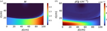
The two-dimensional distribution of: (a) plasma velocity, in units of Mach number; and (b) plasma density, $\rho$
(g cm
$\rho$
(g cm $^{-3}$
), in the stationary state at
$^{-3}$
), in the stationary state at $t = 24 \tau _s$
.
$t = 24 \tau _s$
.

(a) The magnetic field lines at $t =0$
; (b) the magnetic field lines at
$t =0$
; (b) the magnetic field lines at $t = 24 \tau _{s}$
; (c) streamlines of the flow velocity at
$t = 24 \tau _{s}$
; (c) streamlines of the flow velocity at $t = 24 \tau _{s}$
.
$t = 24 \tau _{s}$
.

Similar to the results in Sheth et al. (Reference Sheth, Smolyakov, Deguire, Pande and Yushmanov2025), over tens of sound times, the plasma evolves into the stationary state with the transonic flow and the sonic point at the magnetic throat, as shown in figure 1. The plasma velocity streamlines at $t=24 \tau _s$
are shown in figure 2(c). We observe some fluctuations, which are especially noticeable at the boundary and outside the plasma column, where the plasma density is very low, as can be seen in figures 1(a) and 1(b). However, overall, the plasma flow and magnetic field profiles are rather stable, and the velocity profile follows the theoretical prediction from (4.7), as is discussed in detail below.
$t=24 \tau _s$
are shown in figure 2(c). We observe some fluctuations, which are especially noticeable at the boundary and outside the plasma column, where the plasma density is very low, as can be seen in figures 1(a) and 1(b). However, overall, the plasma flow and magnetic field profiles are rather stable, and the velocity profile follows the theoretical prediction from (4.7), as is discussed in detail below.
One interesting result of these simulations, also noted in Sheth et al. (Reference Sheth, Smolyakov, Deguire, Pande and Yushmanov2025), is the self-consistent adjustment of the magnetic field to the equilibrium conditions that are defined by the pressure, inertial and magnetic field forces. The initial magnetic field given by (6.2), and corresponding to the paraxial approximation of the magnetic field near the axis of a single current coil at $z=z_0$
, is not a faithful vacuum field in the whole domain since it is not current free and
$z=z_0$
, is not a faithful vacuum field in the whole domain since it is not current free and $\boldsymbol{J} \times \boldsymbol{B} \neq 0$
. In our time-dependent simulations here, the magnetic field is also evolved self-consistently, according to the standard ideal one-fluid MHD model (Mignone et al. Reference Mignone, Bodo, Massaglia, Matsakos, Tesileanu, Zanni and Ferrari2007). As the simulations reach stationary state, we observe the modification of the magnetic field, as shown in figure 2: figure 2(a) shows the magnetic field lines from (6.2) at the initial time
$\boldsymbol{J} \times \boldsymbol{B} \neq 0$
. In our time-dependent simulations here, the magnetic field is also evolved self-consistently, according to the standard ideal one-fluid MHD model (Mignone et al. Reference Mignone, Bodo, Massaglia, Matsakos, Tesileanu, Zanni and Ferrari2007). As the simulations reach stationary state, we observe the modification of the magnetic field, as shown in figure 2: figure 2(a) shows the magnetic field lines from (6.2) at the initial time $t=0$
, figure 2(b) shows the modified magnetic field in saturation, around
$t=0$
, figure 2(b) shows the modified magnetic field in saturation, around $t=24\tau _s$
. The velocity streamlines aligned along the magnetic field, as follows from (3.10), are shown in figure 2(c).
$t=24\tau _s$
. The velocity streamlines aligned along the magnetic field, as follows from (3.10), are shown in figure 2(c).
A remarkable property of the self-consistent evolution of plasma flow is the universal profile of the plasma velocity established in the equilibrium. Figure 3 shows the radial $M_r=V_r/c_s$
, the axial
$M_r=V_r/c_s$
, the axial $M_z=V_z/c_s$
and the total
$M_z=V_z/c_s$
and the total $M=\sqrt {V_r^2 + V_z^2}/c_s$
Mach flow numbers at saturation plotted at different axial locations as functions of the radial coordinate. The dotted lines in these figures show the analytical predictions of the plasma velocity based on (4.7) and mapped from the actual (modified) magnetic field at saturation. Here, as seen in figure 2(b), the radial component of the magnetic field is substantial, especially near the end of the nozzle, and the contribution of the radial plasma velocity is large, as shown in figure 3(a). Figure 3(c) demonstrates convincingly that the total plasma velocity
$M=\sqrt {V_r^2 + V_z^2}/c_s$
Mach flow numbers at saturation plotted at different axial locations as functions of the radial coordinate. The dotted lines in these figures show the analytical predictions of the plasma velocity based on (4.7) and mapped from the actual (modified) magnetic field at saturation. Here, as seen in figure 2(b), the radial component of the magnetic field is substantial, especially near the end of the nozzle, and the contribution of the radial plasma velocity is large, as shown in figure 3(a). Figure 3(c) demonstrates convincingly that the total plasma velocity $M=V_\Vert /c_s$
follows the analytical predictions based on (4.7).
$M=V_\Vert /c_s$
follows the analytical predictions based on (4.7).
The Mach numbers shown as functions of the radius: (a) $M_r=V_r/c_s$
; (b)
$M_r=V_r/c_s$
; (b) $M_z=V_z/c_s$
; and (c)
$M_z=V_z/c_s$
; and (c) $M=\sqrt {M_r^2+M_z^2}$
for different axial locations: blue at
$M=\sqrt {M_r^2+M_z^2}$
for different axial locations: blue at $z=1$
cm, orange at
$z=1$
cm, orange at $z=50$
cm, green at
$z=50$
cm, green at $z=78$
cm and red at
$z=78$
cm and red at $98$
cm. The solid lines are the simulation results, and the dotted lines are analytical predictions from (4.7) based on the modified magnetic field at saturation.
$98$
cm. The solid lines are the simulation results, and the dotted lines are analytical predictions from (4.7) based on the modified magnetic field at saturation.

Figure 3 Long description
Three line graphs depict Mach numbers as functions of radius for different axial locations. Panel A: The graph shows the radial Mach number M_r as a function of radius r in centimeters. The lines represent different axial locations: blue at z equals 1 centimeter, orange at z equals 50 centimeters, green at z equals 78 centimeters, and red at z equals 98 centimeters. Solid lines indicate simulation results, while dotted lines show analytical predictions. Panel B: The graph shows the axial Mach number M_z as a function of radius r in centimeters. The lines represent the same axial locations as in Panel A. Solid lines indicate simulation results, while dotted lines show analytical predictions. Panel C: The graph shows the total Mach number M as a function of radius r in centimeters. The lines represent the same axial locations as in Panels A and B. Solid lines indicate simulation results, while dotted lines show analytical predictions.
The axial and radial momentum balance in the stationary state for the same conditions as in figure 3. (a) The axial forces are shown at r = 10 cm; (b) the radial forces are shown at z = 70 cm; (c) the radial components are shown at z = 90 cm; (d) the radial components are shown at z = 98 cm.

The momentum balance for the same conditions as in figure 3 is shown in figure 4. As was noted above, the initial magnetic field from (6.2), is not force free. The self-consistent evolution of the magnetic field, plasma density and flow results in the modification of the magnetic field so that the full momentum balance is satisfied. Axial plasma acceleration $0.5 \rho \partial _z v_z^2$
is supported by the pressure gradient due to plasma expansion,
$0.5 \rho \partial _z v_z^2$
is supported by the pressure gradient due to plasma expansion, $\partial _z p$
, figure 4(a). However, in the converging part of the nozzle, a fraction of the pressure force is compensated by the magnetic stress force
$\partial _z p$
, figure 4(a). However, in the converging part of the nozzle, a fraction of the pressure force is compensated by the magnetic stress force $-(4\pi )^{-1}(\boldsymbol{J} \times \boldsymbol{B})_z$
which opposes the pressure gradient. Note that, in the diverging part of the nozzle, for
$-(4\pi )^{-1}(\boldsymbol{J} \times \boldsymbol{B})_z$
which opposes the pressure gradient. Note that, in the diverging part of the nozzle, for $z\gt 50$
cm, the
$z\gt 50$
cm, the $-(4\pi )^{-1}(\boldsymbol{J} \times \boldsymbol{B})_z$
contribution changes sign and becomes positive, thus increasing the acceleration, the so-called diamagnetic enhancement (Takahashi et al. Reference Takahashi, Lafleur, Charles, Alexander and Boswell2011).
$-(4\pi )^{-1}(\boldsymbol{J} \times \boldsymbol{B})_z$
contribution changes sign and becomes positive, thus increasing the acceleration, the so-called diamagnetic enhancement (Takahashi et al. Reference Takahashi, Lafleur, Charles, Alexander and Boswell2011).
The relative contributions of the radial pressure, magnetic and inertial forces vary along the nozzle. In the first half of the diverging part of the nozzle, at $z=70$
cm, we observe the radial pressure gradient to be mostly balanced by the radial component of the Lorentz force
$z=70$
cm, we observe the radial pressure gradient to be mostly balanced by the radial component of the Lorentz force $-(4\pi )^{-1}(\boldsymbol{J} \times \boldsymbol{B})_r$
, figure 4(b): a typical balance in plasmas without flows. Further downstream, at
$-(4\pi )^{-1}(\boldsymbol{J} \times \boldsymbol{B})_r$
, figure 4(b): a typical balance in plasmas without flows. Further downstream, at $z=90$
cm, the magnetic force
$z=90$
cm, the magnetic force $-(4\pi )^{-1} (\boldsymbol{J} \times \boldsymbol{B})_r$
decreases and starts to change sign along the radial direction, figure 4(c). At the end of the nozzle,
$-(4\pi )^{-1} (\boldsymbol{J} \times \boldsymbol{B})_r$
decreases and starts to change sign along the radial direction, figure 4(c). At the end of the nozzle, $z=98$
cm, the radial magnetic force,
$z=98$
cm, the radial magnetic force, $-(4\pi )^{-1}(\boldsymbol{J} \times \boldsymbol{B})_r$
, changes sign (the red line in figure 4(
d
)), the pressure gradient force becomes small and the magnetic force is mostly balanced by the inertial forces due to the radial flow (the green and orange lines in figure 4(
d
)). The modifications in the momentum balance occur due to plasma acceleration and increasing contributions of the inertial forces due to plasma flow in the curved magnetic field. The snapshots of various contributions to the momentum balance in figure 4 demonstrate that the overall total momentum balance is satisfied rather well, except for some time-dependent fluctuations, which are especially large at the boundary of the plasma column and outside, where the plasma density is small. Generally, these fluctuations are related to the MHD (fast and slow) modes.
$-(4\pi )^{-1}(\boldsymbol{J} \times \boldsymbol{B})_r$
, changes sign (the red line in figure 4(
d
)), the pressure gradient force becomes small and the magnetic force is mostly balanced by the inertial forces due to the radial flow (the green and orange lines in figure 4(
d
)). The modifications in the momentum balance occur due to plasma acceleration and increasing contributions of the inertial forces due to plasma flow in the curved magnetic field. The snapshots of various contributions to the momentum balance in figure 4 demonstrate that the overall total momentum balance is satisfied rather well, except for some time-dependent fluctuations, which are especially large at the boundary of the plasma column and outside, where the plasma density is small. Generally, these fluctuations are related to the MHD (fast and slow) modes.
We further extend our investigation for the case of a purely diverging magnetic nozzle with plasma injected at the maximum of the magnetic field. In this case, we use a force-free (vacuum) magnetic field as the initial state, with the magnetic flux function of the form in (6.5)
 \begin{equation} \psi = \frac {r^2 B_*}{2} \left (1 - \frac {\alpha L}{ \pi r}\cos \left (\frac {2 \pi z}{L}\right ) I_1\left (\frac {2 \pi r}{L}\right )\right )\!, \end{equation}
giving the magnetic field in the form
 \begin{align} B_{r}&=-B_* \alpha \sin \left (\frac {2 \pi z}{L}\right ) I_{1}\left (\frac {2 \pi r}{L}\right )\!, \end{align}
 \begin{align} B_{z}&=B_*\left (1-\alpha \cos \left (\frac {2 \pi z}{L}\right ) I_{0}\left (\frac {2 \pi r}{L}\right )\right )\!. \end{align}
Here, $I_0$
and
$I_0$
and $I_1$
are the modified Bessel functions of the first kind.
$I_1$
are the modified Bessel functions of the first kind.
We consider the simulation box from nozzle throat at z = $50$
to
$50$
to $z=L=100\,\text{cm}$
, with the radial direction
$z=L=100\,\text{cm}$
, with the radial direction $0 \lt r\lt a=20\,\text{cm}$
. To increase the magnetic field divergence we use
$0 \lt r\lt a=20\,\text{cm}$
. To increase the magnetic field divergence we use $\alpha = 0.7$
.
$\alpha = 0.7$
.
The initial state and boundary conditions for plasma injections ( $V_z$
and
$V_z$
and $\rho$
) are the same as in the previous case with (6.3) and (6.4). For isothermal plasmas, we expect that at the nozzle throat
$\rho$
) are the same as in the previous case with (6.3) and (6.4). For isothermal plasmas, we expect that at the nozzle throat $V_z = c_s$
, so that
$V_z = c_s$
, so that $v_0=1$
in (6.3). However, to test the robustness of our simulations, we apply
$v_0=1$
in (6.3). However, to test the robustness of our simulations, we apply $v_0 = 0.1$
at
$v_0 = 0.1$
at $z=50$
cm. In figure 5(c) we observe that, despite the wrong boundary conditions at the throat, the flow quickly transitions to the expected correct value M = 1 over a few computational cells, as was already seen in Sheth et al. (Reference Sheth, Smolyakov, Deguire, Pande and Yushmanov2025). Again, similarly to the previous example of a full nozzle, the expanding nozzle demonstrates the universal profile of the total plasma velocity along the magnetic field in saturation. Figures 6(a) and 6(b) show the radial and axial Mach numbers as functions of the radial coordinate at several axial locations plotted together with the analytical predictions (dotted lines). Figure 6(c), showing the total Mach number along the magnetic field, demonstrates good agreement with the theoretical expression of (4.7) calculated over the modified magnetic field.
$z=50$
cm. In figure 5(c) we observe that, despite the wrong boundary conditions at the throat, the flow quickly transitions to the expected correct value M = 1 over a few computational cells, as was already seen in Sheth et al. (Reference Sheth, Smolyakov, Deguire, Pande and Yushmanov2025). Again, similarly to the previous example of a full nozzle, the expanding nozzle demonstrates the universal profile of the total plasma velocity along the magnetic field in saturation. Figures 6(a) and 6(b) show the radial and axial Mach numbers as functions of the radial coordinate at several axial locations plotted together with the analytical predictions (dotted lines). Figure 6(c), showing the total Mach number along the magnetic field, demonstrates good agreement with the theoretical expression of (4.7) calculated over the modified magnetic field.
(a) Magnetic field lines in the initial state at $t =0$
, (6.5)–(6.7); (b) the magnetic field in saturation at
$t =0$
, (6.5)–(6.7); (b) the magnetic field in saturation at $t = 10 \tau _{s}$
; and (c) streamlines of the flow velocity at
$t = 10 \tau _{s}$
; and (c) streamlines of the flow velocity at $t = 10 \tau _{s}$
.
$t = 10 \tau _{s}$
.

Figure 5 Long description
Panel A: A vector field plot shows magnetic field lines in the initial state at time t equals 0. The horizontal axis is labeled z in centimeters, ranging from 50 to 100. The vertical axis is labeled r in centimeters, ranging from 0 to 20. The magnetic field lines are represented by blue arrows and curves, indicating the direction and magnitude of the magnetic field. Panel B: Another vector field plot displays the magnetic field in saturation at time t equals 10 tau subscript s. The axes and their labels remain the same as in Panel A. The magnetic field lines are again shown with blue arrows and curves, illustrating the changes in the magnetic field over time. Panel C: A vector field plot combined with a color gradient map shows the streamlines of the flow velocity at time t equals 10 tau subscript s. The horizontal axis is labeled z in centimeters, ranging from 50 to 100. The vertical axis is labeled r in centimeters, ranging from 0 to 20. The streamlines are depicted with black arrows, and the color gradient map in the background represents the magnitude of the flow velocity, with a color bar on the right indicating the scale from 1 to 3.
The Mach numbers shown as functions of the radius: (a) $M_r=V_r/c_s$
; (b)
$M_r=V_r/c_s$
; (b) $M_z=V_z/c_s$
; and (c)
$M_z=V_z/c_s$
; and (c) $M=\sqrt {M_r^2+M_z^2}$
for different axial locations: blue at
$M=\sqrt {M_r^2+M_z^2}$
for different axial locations: blue at $z=50$
cm, orange at
$z=50$
cm, orange at $z=51$
cm, green
$z=51$
cm, green $z=75$
cm, red at
$z=75$
cm, red at $z=89$
cm and purple
$z=89$
cm and purple $z=99$
cm. The solid lines are the simulation results, and the dotted lines are analytical predictions from (4.7) based on the modified magnetic field at saturation.
$z=99$
cm. The solid lines are the simulation results, and the dotted lines are analytical predictions from (4.7) based on the modified magnetic field at saturation.

In the case of a force-free configuration of the initial magnetic field, the modification to the magnetic field from the initial state in figure 5(a) to the saturation in figure 5(b) is less noticeable, however, it remains important, especially in the radial direction. In the axial direction, at $r=6$
cm, the contribution of the magnetic force to plasma acceleration remains small, and the main effect is plasma acceleration by the pressure force in the axial direction, figure 7(a). Radially, near the beginning of the nozzle, at
$r=6$
cm, the contribution of the magnetic force to plasma acceleration remains small, and the main effect is plasma acceleration by the pressure force in the axial direction, figure 7(a). Radially, near the beginning of the nozzle, at $z=60$
cm, the radial pressure gradient is balanced by the magnetic pressure force, and the inertial contributions are small, figure 7(a). Further down the nozzle, at
$z=60$
cm, the radial pressure gradient is balanced by the magnetic pressure force, and the inertial contributions are small, figure 7(a). Further down the nozzle, at $z=80$
cm, the magnetic force, shown by the red line in figure 7(c), starts to change sign across the radial direction. At the end of the nozzle, at
$z=80$
cm, the magnetic force, shown by the red line in figure 7(c), starts to change sign across the radial direction. At the end of the nozzle, at $z=90$
cm, the pressure terms are less important and the main balance is between the inertial terms due to the radial flows (shown by the orange and green lines in figure 7
d) and the magnetic pressure force (the red line in figure 7
d).
$z=90$
cm, the pressure terms are less important and the main balance is between the inertial terms due to the radial flows (shown by the orange and green lines in figure 7
d) and the magnetic pressure force (the red line in figure 7
d).
The axial and radial momentum balance for the magnetic nozzle as in figure 5. (a) The axial forces at $r =6$
cm shown as a function of
$r =6$
cm shown as a function of $z$
; (b) the radial forces at
$z$
; (b) the radial forces at $z = 60\,\text{cm}$
; (c) the radial forces at
$z = 60\,\text{cm}$
; (c) the radial forces at $z = 80$
cm; and (d) the radial forces at
$z = 80$
cm; and (d) the radial forces at $z = 90$
cm.
$z = 90$
cm.

Figure 7 Long description
The image contains four line graphs depicting the axial and radial momentum balance for a magnetic nozzle. Panel A: A line graph shows the axial forces at a radius of 6 centimeters as a function of the axial position z. The x-axis represents the axial position z in centimeters, and the y-axis represents the axial force Fz in dyn per cubic centimeter. The graph includes multiple lines representing different components of the force, such as partial pressure, plasma pressure, and magnetic field interactions. Panel B: A line graph shows the radial forces at an axial position of 60 centimeters as a function of the radial position r. The x-axis represents the radial position r in centimeters, and the y-axis represents the radial force Fr in dyn per cubic centimeter. The graph includes multiple lines representing different components of the force. Panel C: A line graph shows the radial forces at an axial position of 80 centimeters as a function of the radial position r. The x-axis represents the radial position r in centimeters, and the y-axis represents the radial force Fr in dyn per cubic centimeter. The graph includes multiple lines representing different components of the force. Panel D: A line graph shows the radial forces at an axial position of 90 centimeters as a function of the radial position r. The x-axis represents the radial position r in centimeters, and the y-axis represents the radial force Fr in dyn per cubic centimeter. The graph includes multiple lines representing different components of the force.
The component of the Lorentz force due to the radial magnetic field and azimuthal current, $-(4\pi )^{-1}(\boldsymbol{J} \times \boldsymbol{B})_z=(4\pi )^{-1}J_\phi B_r$
, enters the axial acceleration and is related to the so-called the diamagnetic enhancement of the thrust in the propulsive magnetic nozzle (Takahashi et al. Reference Takahashi, Lafleur, Charles, Alexander and Boswell2011; Fruchtman et al. Reference Fruchtman, Takahashi, Charles and Boswell2012; Correyero et al. Reference Correyero, Merino, Elias, Jarrige, Packan and Ahedo2019). The azimuthal current is also involved in the radial momentum balance,
$-(4\pi )^{-1}(\boldsymbol{J} \times \boldsymbol{B})_z=(4\pi )^{-1}J_\phi B_r$
, enters the axial acceleration and is related to the so-called the diamagnetic enhancement of the thrust in the propulsive magnetic nozzle (Takahashi et al. Reference Takahashi, Lafleur, Charles, Alexander and Boswell2011; Fruchtman et al. Reference Fruchtman, Takahashi, Charles and Boswell2012; Correyero et al. Reference Correyero, Merino, Elias, Jarrige, Packan and Ahedo2019). The azimuthal current is also involved in the radial momentum balance, $-(4\pi )^{-1}(\boldsymbol{J} \times \boldsymbol{B})_r=-(4\pi )^{-1}J_\phi B_z$
, that includes the radial pressure gradient and inertial terms,
$-(4\pi )^{-1}(\boldsymbol{J} \times \boldsymbol{B})_r=-(4\pi )^{-1}J_\phi B_z$
, that includes the radial pressure gradient and inertial terms, $0.5\rho \partial _r V_r^2+\rho V_z\partial _z V_r$
. In the paraxial approximation, the contribution of the inertial force due to the radial velocity is omitted (Fruchtman et al. Reference Fruchtman, Takahashi, Charles and Boswell2012). Our analysis shows that the inertial forces can be essential, especially at the exit part of the nozzle, where the velocity is large and magnetic field lines are strongly diverging due to large expansion. At these locations, the inertial force due to the radial flow is significant, replacing the pressure gradient force, and even change sign, as shown by the orange and green lines in figures 4(
d
) and 7(
d
). It is worth noting that, typically, the contribution of the azimuthal current to the axial acceleration is calculated for the diverging part of the nozzle, where
$0.5\rho \partial _r V_r^2+\rho V_z\partial _z V_r$
. In the paraxial approximation, the contribution of the inertial force due to the radial velocity is omitted (Fruchtman et al. Reference Fruchtman, Takahashi, Charles and Boswell2012). Our analysis shows that the inertial forces can be essential, especially at the exit part of the nozzle, where the velocity is large and magnetic field lines are strongly diverging due to large expansion. At these locations, the inertial force due to the radial flow is significant, replacing the pressure gradient force, and even change sign, as shown by the orange and green lines in figures 4(
d
) and 7(
d
). It is worth noting that, typically, the contribution of the azimuthal current to the axial acceleration is calculated for the diverging part of the nozzle, where $B_r$
is positive. In the converging part,
$B_r$
is positive. In the converging part, $B_r$
is negative, and the contribution due to the azimuthal current can be detrimental to the thrust. However, the diverging part of the nozzle improves plasma confinement, thus increasing the density, and the net effect of the azimuthal currents on the thrust in the converging–diverging nozzle has to be determined self-consistently. The thrust calculations in application to the propulsion systems are beyond the scope of this work.
$B_r$
is negative, and the contribution due to the azimuthal current can be detrimental to the thrust. However, the diverging part of the nozzle improves plasma confinement, thus increasing the density, and the net effect of the azimuthal currents on the thrust in the converging–diverging nozzle has to be determined self-consistently. The thrust calculations in application to the propulsion systems are beyond the scope of this work.
The diamagnetic modification of the magnetic field by expanding plasmas has been observed experimentally in large plasma pressure $\beta =8\pi \rho /B^2 \geqslant 1$
conditions (Stenzel & Urrutia Reference Stenzel and Urrutia2000; Corr & Boswell Reference Corr and Boswell2007; Roberson, Winglee & Prager Reference Roberson, Winglee and Prager2011) up to complete cancellation of the external field and formation of the magnetic holes. Here, we consider a low plasma pressure
$\beta =8\pi \rho /B^2 \geqslant 1$
conditions (Stenzel & Urrutia Reference Stenzel and Urrutia2000; Corr & Boswell Reference Corr and Boswell2007; Roberson, Winglee & Prager Reference Roberson, Winglee and Prager2011) up to complete cancellation of the external field and formation of the magnetic holes. Here, we consider a low plasma pressure $\beta \ll 1$
, and observe essential modifications of the magnetic field since the initial vacuum magnetic field is force free and the force from the magnetic pressure tensor is zero in the initial state. When plasma is present, the magnetic field is modified, and the plasma pressure radial gradient force becomes balanced by the magnetic pressure tensor force, as in the magnetic nozzle at
$\beta \ll 1$
, and observe essential modifications of the magnetic field since the initial vacuum magnetic field is force free and the force from the magnetic pressure tensor is zero in the initial state. When plasma is present, the magnetic field is modified, and the plasma pressure radial gradient force becomes balanced by the magnetic pressure tensor force, as in the magnetic nozzle at $z=60$
cm shown in figure 7(b). At other locations in the magnetic nozzle, the magnetic pressure tensor force may change sign, as in figures 7(c) and 7(d), and be balanced by the inertial forces related to the accelerated plasma flow, as in figure 7(d). Essential modifications of the magnetic field forces shown at different locations in the magnetic nozzle in figure 7 are not necessarily accompanied by large changes of the magnetic field amplitude, such as those shown in the transition from figures 2(a) and 2(b). The latter occurs because the initial field in figure 2(a) was not force free. The initial magnetic field was modified in the presence of plasma and brought into the equilibrium state consistent with the plasma pressure gradient and inertial forces.
$z=60$
cm shown in figure 7(b). At other locations in the magnetic nozzle, the magnetic pressure tensor force may change sign, as in figures 7(c) and 7(d), and be balanced by the inertial forces related to the accelerated plasma flow, as in figure 7(d). Essential modifications of the magnetic field forces shown at different locations in the magnetic nozzle in figure 7 are not necessarily accompanied by large changes of the magnetic field amplitude, such as those shown in the transition from figures 2(a) and 2(b). The latter occurs because the initial field in figure 2(a) was not force free. The initial magnetic field was modified in the presence of plasma and brought into the equilibrium state consistent with the plasma pressure gradient and inertial forces.
The enhanced plasma magnetism could be directly observed in the magnetic nozzle extended to the Alfvénic point, where the magnetic field is low, and the kinetic energy of accelerated plasma becomes comparable to the magnetic energy, $\rho V^2/2 \sim B^2/4\pi$
, so that the plasma flow can stretch the magnetic field (Takahashi & Ando Reference Takahashi and Ando2017; Takahashi et al. Reference Takahashi, Charles and Boswell2023a
). The plasma flow in the extended magnetic nozzle that included the Alfvénic and fast-MHD points was analysed with the MHD model in Smolyakov et al. (Reference Smolyakov, Sabo, Krasheninnikov and Yushmanov2025).
$\rho V^2/2 \sim B^2/4\pi$
, so that the plasma flow can stretch the magnetic field (Takahashi & Ando Reference Takahashi and Ando2017; Takahashi et al. Reference Takahashi, Charles and Boswell2023a
). The plasma flow in the extended magnetic nozzle that included the Alfvénic and fast-MHD points was analysed with the MHD model in Smolyakov et al. (Reference Smolyakov, Sabo, Krasheninnikov and Yushmanov2025).
7. Summary and discussion
We have shown analytically here that, in the absence of plasma rotation and an azimuthal magnetic field, the plasma dynamics in the magnetic nozzle can be described by the one-fluid MHD model. Projecting the momentum balance on the direction of the total magnetic field, we have obtained the equation for plasma acceleration along the magnetic field. The structure of this equation is similar (or identical) to the equations obtained previously in the one-dimensional paraxial models (Manheimer & Fernsler Reference Manheimer and Fernsler2001; Fruchtman Reference Fruchtman2006; Smolyakov et al. Reference Smolyakov, Sabo, Yushmanov and Putvinskii2021). While the equation remains one-dimensional, it is now written along the magnetic field with the length parameterised by the field amplitude. The shape of the magnetic surface is determined by the generalised GS equation that includes the inertial forces and is obtained by the projection of the momentum balance on the direction normal to the magnetic surfaces. Our numerical simulations confirm that, under a wide choice of boundary conditions, the transonic flow along the magnetic surface is very robust so that the local value of the velocity is determined by the magnetic field amplitude, and the velocity profile agrees well with the analytical solution. We note that similar results were reported in experiments (Pioch Reference Pioch2024).
Therefore, the problem of the dynamical equilibrium (stationary state with a finite flow) in the magnetic nozzle is decoupled into two parts: (a) the equilibrium along the magnetic field, where plasma is accelerated by the pressure gradient along the (curved) magnetic field, and (b) the transversal (normal to the magnetic surfaces) equilibrium, in which the pressure gradient and inertial forces (due to the plasma flow along the curvilinear magnetic field) are balanced by the magnetic pressure (stress) forces. The inertia forces due to ram pressure ( $\sim V_\Vert ^2$
) contribute both to the parallel direction, as the parallel gradient force along the magnetic field,
$\sim V_\Vert ^2$
) contribute both to the parallel direction, as the parallel gradient force along the magnetic field, $V_\Vert (\partial /\partial s) V_\Vert$
, and to the transverse direction, as the centrifugal force due to the curvature of the magnetic field,
$V_\Vert (\partial /\partial s) V_\Vert$
, and to the transverse direction, as the centrifugal force due to the curvature of the magnetic field, $V_{\Vert }^{2}\boldsymbol{\nabla }\psi \boldsymbol{\cdot } ( \boldsymbol{b}\boldsymbol{\cdot }{\boldsymbol{\nabla }}) \boldsymbol{b}$
, where
$V_{\Vert }^{2}\boldsymbol{\nabla }\psi \boldsymbol{\cdot } ( \boldsymbol{b}\boldsymbol{\cdot }{\boldsymbol{\nabla }}) \boldsymbol{b}$
, where $V_\Vert$
is the plasma velocity along the magnetic field,
$V_\Vert$
is the plasma velocity along the magnetic field, $\psi$
is the magnetic flux function for the poloidal magnetic field and
$\psi$
is the magnetic flux function for the poloidal magnetic field and $\boldsymbol{b}$
is a unit vector of the magnetic field.
$\boldsymbol{b}$
is a unit vector of the magnetic field.
Our simulations demonstrate the self-consistent modifications of the magnetic field: the velocity profiles shown in figure 3(c) and in figure 6(c) follow the analytical predictions from (4.7) using the modified magnetic field in the saturated state, as had already been demonstrated earlier in Sheth et al. (Reference Sheth, Smolyakov, Deguire, Pande and Yushmanov2025). In the saturated state, the pressure gradient, inertial and magnetic stress (from the modified field) terms are all of the same order. We note that diamagnetic contributions to the thrust, associated with the radial pressure gradient in Takahashi et al. (Reference Takahashi, Lafleur, Charles, Alexander and Boswell2011) and Fruchtman et al. (Reference Fruchtman, Takahashi, Charles and Boswell2012), also include the inertial contributions due to the plasma flow.
It has been noted that the sonic singularity in plasma acceleration in the Hall thruster introduces some features similar to the supersonic flow in the Laval nozzle (Fruchtman, Fisch & Raitses Reference Fruchtman, Fisch and Raitses2001). In Hall thruster, the dissipation, ionisation and losses may effectively create conditions equivalent to a converging and diverging geometry of the nozzle (Fruchtman et al. Reference Fruchtman, Fisch and Raitses2001; Fruchtman Reference Fruchtman2003; Meige et al. Reference Meige, Boswell, Charles and Turner2005; Romadanov et al. Reference Romadanov, Smolyakov, Sorokina, Andreev and Marusov2020; Lafleur & Chabert Reference Lafleur and Chabert2024). Similar analogy exists in the supersonic acceleration of the solar wind in the central gravity field (Cranmer Reference Cranmer2004) and plasma flow toward the cylindrical probe (Fruchtman, Zoler & Makrinich Reference Fruchtman, Zoler and Makrinich2011). Therefore, the universal features of supersonic plasma acceleration discussed in this manuscript could be relevant to plasma acceleration in Hall thrusters and the self-consistent modifications of the magnetic field (Merino & Ahedo Reference Merino and Ahedo2016) and associated magnetic stress could be important for the calculations of the upper thrust limits for electric propulsion devices such as Hall thruster (Simmonds & Raitses Reference Simmonds and Raitses2021; Simmonds, Raitses & Smolyakov Reference Simmonds, Raitses and Smolyakov2023).
Plasma rotation and the azimuthal magnetic field due to the poloidal current are among the most important effects neglected in the above simple picture of the equilibrium of a flowing plasma. Within the approximations of the ideal (non-dissipative) plasmas and full azimuthal symmetry, the ion deviations from the magnetic field are related to the azimuthal rotation. Plasma rotation and the azimuthal magnetic field provide additional contributions to the acceleration and equilibrium since both can be additional reservoirs of the energy for plasma acceleration as well as energy sinks when the rotation and associated azimuthal magnetic field are induced by flowing plasmas (Smolyakov et al. Reference Smolyakov, Sabo, Krasheninnikov and Yushmanov2025). These effects can be analysed within the one-fluid MHD, as was done in Smolyakov et al. (Reference Smolyakov, Sabo, Krasheninnikov and Yushmanov2025). However, the one-fluid MHD model still assumes that, in the stationary state, plasma flow in the poloidal plane follows the poloidal magnetic field. This is not true in the two-fluid model with Hall effects included; there, plasma rotation directly results in the deviation of the flow from the magnetic surfaces, as per (3.3).
Therefore, in the current model, we do not consider the plasma detachment from the magnetic field (Breizman, Tushentsov & Arefiev Reference Breizman, Tushentsov and Arefiev2008; Merino & Ahedo Reference Merino and Ahedo2014), which is important for propulsion. In fusion applications (Bagryansky et al. Reference Bagryansky, Beklemishev and Postupaev2019; Gota et al. Reference Gota2021; Endrizzi et al. Reference Endrizzi2023), plasma detachment affects the energy fluxes to the walls and defines the optimal geometry of the magnetic field.
Dissipative and radial transport effects (Fruchtman, Makrinich & Ashkenazy Reference Fruchtman, Makrinich and Ashkenazy2005; Onofri et al. Reference Onofri, Yushmanov, Dettrick, Barnes, Hubbard and Tajima2017), as well as such kinetic effects as electron and ion pressure anisotropy and ion finite Larmor radius, also will have to be considered. We have shown in drift-kinetic theory (Tyushev et al. Reference Tyushev, Smolyakov, Sabo, Groenewald, Necas and Yushmanov2025) that universal profiles of plasma acceleration agree well with the fluid theory in bulk plasma but deviations appear closer to the boundaries, where quasineutrality is not maintained. Additional forces due to the ion pressure tensor at large ion Larmor radius and due to energetic ions will contribute to the equilibria considered here.
Acknowledgements
A.S. acknowledges useful discussions with M. Merino, R. Pioch, V. Désangles and P. Chabert. This work is supported in part by the Natural Sciences and Engineering Research Council of Canada (NSERC). The computational resources were provided by Digital Research Alliance of Canada.
Editor Cary Forest thanks the referees for their advice in evaluating this article.
Declaration of interests
The authors report no conflicts of interest.
Data availability
The data that support the findings of this study are available from the corresponding author upon reasonable request.

 ρ
ρ −3
−3 t=24τs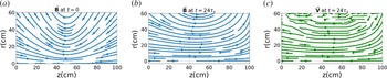
 t=0
t=0 t=24τs
 t=24τs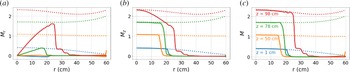
 Mr=Vr/cs
 Mz=Vz/cs
 M=Mr2+Mz2
 z=1
z=1 z=50
z=50 z=78
z=78 98
98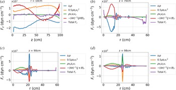

 t=0
t=0 t=10τs
 t=10τs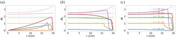
 Mr=Vr/cs
 Mz=Vz/cs
 M=Mr2+Mz2
 z=50
z=50 z=51
z=51 z=75
z=75 z=89
z=89 z=99
z=99
 r=6
r=6 z
z z=60cm
 z=80
z=80 z=90
z=90
 Open access

