


1. Introduction
Most of the large-scale turbulent flow systems in nature and many industrial flows are driven by temperature-induced buoyancy. Examples include the Earth's outer core, its atmosphere or the flow in the convection zone of the Sun and other stars. Despite being highly turbulent, these flows often exhibit coherent structures on large scales, due to intrinsic mechanisms, geometric confinement and the interaction of both.
Since such flows involve large spatial scales and intense turbulence, and hence are difficult to investigate, researchers often study the fundamental physics of thermal convection in idealised model systems, with a reduced number of control parameters. One of the best investigated model systems is Rayleigh–Bénard convection (RBC), where a horizontal fluid layer of height  $H$ is heated from below and cooled from above (Bénard Reference Bénard1900; Rayleigh Reference Rayleigh1916; Kadanoff Reference Kadanoff2001; Ahlers, Grossmann & Lohse Reference Ahlers, Grossmann and Lohse2009; Lohse & Xia Reference Lohse and Xia2010). Most investigations study the RBC system under Oberbeck–Boussinesq conditions, where the temperature difference between the bottom and top boundary is small enough so that relevant fluid properties are constant everywhere in the domain (Oberbeck Reference Oberbeck1879; Boussinesq Reference Boussinesq1903; Spiegel & Veronis Reference Spiegel and Veronis1960). Solely the mass density is assumed to depend linearly on the temperature which is accounted for in the buoyancy term in the momentum equation. In this case, the system is governed by two dimensionless control parameters. The first parameter is the Rayleigh number
 \begin{equation} {\textit{Ra}} = \frac{g\alpha \Delta T H^3}{\nu\kappa}, \end{equation}
which is the ratio between the driving (buoyancy) and the damping mechanisms (diffusion of heat and momentum). The second control parameter is the Prandtl number
 \begin{equation} {\textit{Pr}} = \frac{\nu}{\kappa}, \end{equation}
which is the ratio of the two damping mechanisms. Here,  $\Delta T = T_b - T_t$ denotes the temperature difference between the bottom and top plates, $g$ the gravitational acceleration, $\alpha$ the thermal isobaric expansion coefficient, $\nu$ the kinematic viscosity and $\kappa$ is the thermal diffusivity of the fluid. All fluid properties are evaluated at the mean temperature $T_m = (T_t + T_b)/2$.
For small Ra the flow is laminar and in horizontally extended systems exhibits periodic patterns in horizontal direction with a wavelength  $\lambda \approx 2H$ (Bodenschatz, Pesch & Ahlers Reference Bodenschatz, Pesch and Ahlers2000). With increasing Ra the flow becomes first chaotic and finally turbulent (Krishnamurti Reference Krishnamurti1973; Ahlers et al. Reference Ahlers, Grossmann and Lohse2009). In turbulent RBC, coherent flow patterns do exist and become visible upon time averaging, so that fast fluctuations on smaller scales average out (Hartlep, Tilgner & Busse Reference Hartlep, Tilgner and Busse2003; Bailon-Cuba, Emran & Schumacher Reference Bailon-Cuba, Emran and Schumacher2010). The wavelength of the coherent structures was found to increase with Ra asymptotically towards $\lambda \rightarrow 6H$ (Pandey, Scheel & Schumacher Reference Pandey, Scheel and Schumacher2018; Stevens et al. Reference Stevens, Blass, Zhu, Verzicco and Lohse2018). The exact size as well as the properties of these coherent structures is influenced by the aspect ratio between the width $D$ of the convection domain and its height
 \begin{equation} \varGamma= D/H. \end{equation}
For  $\varGamma \lesssim 32$ confinement effects cause $\lambda$ to decrease (Pandey et al. Reference Pandey, Scheel and Schumacher2018; Stevens et al. Reference Stevens, Blass, Zhu, Verzicco and Lohse2018). At $\varGamma =1$, a case that many investigations have focused on in the past (Ahlers et al. Reference Ahlers, Grossmann and Lohse2009), the largest flow structure is a single large-scale convection roll (LSC), in which warm fluid rises along one side and cool fluid sinks at the opposite side, and which spans through the entire convection container.
The Nusselt number  $ {\textit {Nu}} = {qH}/{(\chi \Delta T)}$, as a measure of the non-dimensional heat flux, is one of the most important global response parameters that is affected by the number and morphology of the coherent turbulent structures (Wang et al. Reference Wang, Verzicco, Lohse and Shishkina2020). Here, $q$ denotes the vertical heat flux and $\chi$ the heat conductivity of the fluid. Another global response parameter is the Reynolds number
 \begin{equation} {\textit{Re}} =\frac{UH}{\nu}, \end{equation}
with  $U=\sqrt {\langle u^2+v^2+w^2\rangle }$ being the root mean square velocity, averaged over the entire volume as well as over time. In the past, researchers have developed models describing the relation between control and response parameters, i.e. $ {\textit {Nu}}( {\textit {Ra}}, {\textit {Pr}},\varGamma )$ and $ {\textit {Re}}( {\textit {Ra}}, {\textit {Pr}},\varGamma )$ (Malkus Reference Malkus1954; Kraichnan Reference Kraichnan1962; Grossmann & Lohse Reference Grossmann and Lohse2000, Reference Grossmann and Lohse2001; Stevens et al. Reference Stevens, van der Poel, Grossmann and Lohse2013; Shishkina et al. Reference Shishkina, Emran, Grossmann and Lohse2017). Because the global heat flux can rather easily be measured, experiments have so far predominantly focused on measurements of $ {\textit {Nu}}$ (e.g. Chavanne et al. Reference Chavanne, Chilla, Castaing, Hebral, Chabaud and Chaussy1997; Niemela et al. Reference Niemela, Skrbek, Sreenivasan and Donnelly2000; Weiss & Ahlers Reference Weiss and Ahlers2011; He et al. Reference He, Funfschilling, Bodenschatz and Ahlers2012). Investigation of the Reynolds number or the velocity field in turn are much more challenging and therefore have mostly been conducted in direct numerical simulation (DNS) (Schumacher Reference Schumacher2009; Kooij et al. Reference Kooij, Botchev, Frederix, Geurts, Horn, Lohse, van der Poel, Shishkina, Stevens and Verzicco2018) or only rather sparsely using localised (Puits, Resagk & Thess Reference du Puits, Resagk and Thess2009; He et al. Reference He, van Gils, Bodenschatz and Ahlers2015) or indirect measurement (Brown & Ahlers Reference Brown and Ahlers2007; Funfschilling, Brown & Ahlers Reference Funfschilling, Brown and Ahlers2008).
While planar measurements of two velocity components along cross-sectional slices have been achieved already two decades ago by using particle image velocimetry (e.g. Sun, Xia & Tong Reference Sun, Xia and Tong2005; Wedi et al. Reference Wedi, Moturi, Funfschilling and Weiss2022), the improvement of cameras, computational power and computational algorithms allow us nowadays to measure all three velocity components in complete sample volumes with high spatial resolution by using Lagrangian particle tracking (Schanz, Gesemann & Schröder Reference Schanz, Gesemann and Schröder2016; Schröder & Schanz Reference Schröder and Schanz2023). In this context, high-density particle tracking has recently been employed in RBC by Paolillo et al. (Reference Paolillo, Greco, Astarita and Cardone2021) to study the LSC in a cylindrical RBC cell of aspect ratio  $\varGamma =1/2$. For this, they interpolated the velocity from each particle onto a regular grid, and investigated the dynamics of the LSC in terms of proper orthogonal modes.
In this paper we study Lagrangian particle tracks in densely seeded RBC containers of aspect ratios ranging from  $\varGamma =1$ to $\varGamma =16$. Not only do we want to access the global Reynolds number but we further want to investigate how the large-scale Eulerian flow structures are reflected in Lagrangian statistical properties. While flows are most often observed and described in the Eulerian view, i.e. from a stationary viewpoint, there are good reasons to study flows from the Lagrangian perspective, i.e. at positions that are advected with the flow. The Lagrangian view is not only beneficial if one is interested in the dispersion of tracer particles (e.g. in the context of pollutants or nutrients) but with the emergence of modern particle tracking techniques, flow properties are directly accessible. Ideally, in a spatially confined statistically steady turbulent flow, following a single particle over sufficiently long time would allow us to determine all relevant statistical properties. For this reason, Lagrangian particle tracking with low seeding density has been used for over two decades to measure Lagrangian statistics in homogeneous isotropic turbulence (Porta et al. Reference Porta, Voth, Crawford, Alexander and Bodenschatz2001; Bourgoin et al. Reference Bourgoin, Ouellette, Xu, Berg and Bodenschatz2006).
However, since RBC is a model system for turbulent convection, we also want to understand how buoyancy affects these statistics. A theoretical framework for turbulent flows as laid out by Kolmogorov (Pope Reference Pope2000) assumes isotropy and homogeneity, which are not given here. Therefore, no theoretical predictions for Lagrangian statistical properties exist so far. Nevertheless, some concepts from homogeneous isotropic turbulence (HIT) are applicable to thermal convection as well.
For example, similar to HIT, in RBC the large eddies (given by size of the coherent superstructures) break and transfer kinetic energy towards smaller eddies, which dissipate into heat at an average rate  $\varepsilon$ on length scales similar to the Kolmogorov length $\eta _k$. Since the energy is provided as potential energy caused by the temperature difference between the bottom and the top plate, one can analytically calculate this dissipation rate as (Ahlers et al. Reference Ahlers, Grossmann and Lohse2009)
 \begin{equation} \varepsilon = \frac{\nu^3}{H^4}(Nu-1){\textit{Ra}} {\textit{Pr}}^{{-}2} \end{equation}
and subsequently the Kolmogorov length scale as
 \begin{equation} \eta_k = \left(\frac{\nu^3}{\varepsilon}\right)^{1/4} = H {\textit{Pr}}^{1/2}(Nu-1)^{{-}1/4} {\textit{Ra}}^{{-}1/4}. \end{equation}
One significant difference to HIT is, however, that  $\varepsilon$ is inhomogeneously distributed. Due to the enhanced shear, the dissipation rate is significantly larger in thin boundary layers at the top and the bottom than in the bulk.
Lagrangian properties of RBC have also been studied in the past both in DNS by Schumacher (Reference Schumacher2009), Emran & Schumacher (Reference Emran and Schumacher2010), Schütz & Bodenschatz (Reference Schütz and Bodenschatz2016) and in experiments by Ni, Huang & Xia (Reference Ni, Huang and Xia2012), Ni & Xia (Reference Ni and Xia2013) and Liot et al. (Reference Liot, Martin-Calle, Gay, Salort, Chillà and Bourgoin2019). While these studies have provided valuable information, they were bound by constraints that have just been lifted by modern experimental techniques. For example, Liot et al. (Reference Liot, Martin-Calle, Gay, Salort, Chillà and Bourgoin2019) studied particle dispersion over long times, which demanded long tracks. Therefore, they were bound to low seeding densities by their tracking algorithm and could not study sufficiently well the dependency of particle separation on the initial separation distance. On the other hand, Ni & Xia (Reference Ni and Xia2013) have studied in detail particle-pair dispersion for small initial separation but had only limited data on the regime where Richardson dispersion (Richardson Reference Richardson1926) was expected.
While small-scale Eulerian properties of turbulent thermal convection are only poorly understood, this is even more true for the Lagrangian properties (Lohse & Xia Reference Lohse and Xia2010). The lack of any theoretical framework is also due to a lack of experimental or numerical data available. In experiments like the one we have recently reported about (Bosbach et al. Reference Bosbach, Schanz, Godbersen and Schröder2021; Godbersen et al. Reference Godbersen, Bosbach, Schanz and Schröder2021; Weiss et al. Reference Weiss, Schanz, Erdogdu, Schröder and Bosbach2023), we could track particles for up to 2000 free-fall times with a particle density of approximately 0.14/ $\eta _k^3$. From these experiments, we now have a unique data set which, if properly analysed, can enhance our understanding of Lagrangian statistical properties in thermal turbulence and support the development of statistical models to describe such flows. In the following, we provide a very thorough analysis of Lagrangian particle statistics in RBC for three different aspect ratios ( $\varGamma \in \{1,8,16\}$), two different Prandtl numbers ( $ {\textit {Pr}}\in \{0.7, 7\}$) and Rayleigh numbers from $ {\textit {Ra}} = 1.1\times 10^6$ up to $1.53\times 10^9$.
The paper is structured as follows. In the next section, we describe the experimental set-ups and give a brief overview of the particle tracking algorithm. In § 3.1 we compare the vertical velocity profiles for different measurements as well as the Reynolds number as a function of Pr and Ra. We then discuss the vertical distribution of the energy dissipation rates in § 3.2 and analyse the velocity autocorrelation for the vertical and horizontal component in § 3.3. In § 3.4 we analyse single particle displacements, while the Lagrangian velocity-structure function and particle-pair dispersion are presented and discussed in § 3.5 and in § 3.6, respectively. We close the paper with a discussion and a summary.
2. Experimental set-up
The data presented in the following were acquired in two different experimental set-ups. One with a large aspect ratio and a square horizontal cross-section, which in the following will be abbreviated SQR, and another apparatus with a cylindrical cell of aspect ratio  $\varGamma = 1$, abbreviated as CYL. An overview of the datasets discussed in this paper is given in table 1
Overview of the experiments conducted.

2.1. The square, large aspect ratio cell – SQR
The SQR, which is described in detail in Weiss et al. (Reference Weiss, Schanz, Erdogdu, Schröder and Bosbach2023) and sketched in figure 1(a), consists of a rectangular convection cell with a square horizontal cross-section of side length  $D=320$ mm. The sidewalls are made out of transparent Plexiglas and also act as spacers which determine the cell height. It can easily be exchanged and therefore the apparatus allows experiments with different $H$ without much additional effort. Here, we present results from experiments using sidewalls of height $H=20$ and $H=40$ mm resulting in $\varGamma =16$ and $\varGamma =8$.
(a) Sketch of the experimental set-up for the rectangular cell (SQR8 and SQR16). (b) Overview of the experimental set-up for the cylindrical cell with  $\varGamma =1$ (CYL1).

The fluid is confined from below by a bottom plate with a thickness of 30 mm, made out of aluminium and electrically heated at its bottom with a carbon fibre fabric. A 15-cm-thick polypropylene foam underneath the plate prevented heat loss to the bottom. The top plate was a 0.5-mm-thick borosilicate glass which was cooled on its top with temperature-controlled water, whose temperature was regulated by a chiller to within  ${\pm }10$ mK. The working fluid and the cooling water were connected with a thin capillary that allowed pressure equilibration between both chambers without affecting the flow inside the convection cell.
The entire cell was levelled to within  $0.2^\circ$ with respect to gravity. The temperature of the bottom ( $T_b$) was measured via four evenly distributed thermistors (Pt1000) that were embedded in blind holes drilled from underneath up to roughly 1 mm below the bottom plate's upper surface. The top plate temperature was deduced from temperature measurements inside the cooling liquid. For this we placed four thermistors from above into the cooling water such that two thermistors measured the temperature of the inflow while the other two measured the temperature of the outflow of the water inside the cooling chamber (short vertical green lines in figure 1a). The mass flux of cooling fluid was sufficiently large to avoid temperature gradients across the top plate. The temperature drop across the top plate due to its finite thermal conductivity was taken into account.
The working fluid was distilled water with sodium chloride added (0.25 per cent in mass) in order to match its density to that of the seeding particles. As seeding particles, we used  $\sim 50-\mathrm {\mu }$m-large fluorescent polyethylene microspheres (UVPMS-BO-1.00 by Cospheric LLC). Illumination was done from the side via two pulsed ultraviolet (UV) light emitting diode (LED) arrays (LED Flashlight 300 by LaVision). The UV light was also reflected back by plane mirrors at the opposite sidewalls in order to achieve illumination of the particles from all sides. The particles absorbed the UV light and emitted visible light at wavelengths longer than 580 nm. Therefore, scattered UV light from the sides or the bottom plate was filtered out by a long-pass filter (Perspex ‘orange’, 550 nm, 3 mm thick) placed above the top plate. Images of the particles were captured from six different angles in the range 7 $^\circ$ to 28 $^\circ$ with a total aperture of approximately 55 $^\circ$ using scientific complementary metal-oxide semiconductor (sCMOS) cameras (Imager sCMOS by LaVision, $2560\times 2160$ pixels). Since the flow velocity is not very fast, images were taken with up to 19 Hz, which is 19 times faster than the typical free-fall time $t_{f} = \sqrt {H/(\alpha g \Delta T)}$ of around 1 s (see table 1).
2.2. The cylindrical cell with small aspect ratio – CYL
The set-up of the small aspect ratio cell is shown in figure 1(b) and has previously been described in more detail in Bosbach et al. (Reference Bosbach, Schanz, Godbersen and Schröder2021, Reference Bosbach, Schanz, Godbersen and Schröder2022). Convection takes place in a cylindrical container of diameter and height  $D=H = 1.1$ m, resulting in an aspect ratio $\varGamma =1$. By using air at atmospheric pressure as working fluid, Rayleigh numbers up to ${\textit {Ra}} = 10^9$ were reached at $ {\textit {Pr}} = 0.7$ by applying moderate temperature differences of up to $\Delta T =12$ K.
A sandwich of an aluminium plate with a thickness of 15 mm, heated electrically from below by a network of carbon and glass fibre mats, in turn thermally insulated by a layer of 6-cm-thick Styrofoam, was used as heating plate. To allow for LED illumination from the top, a transparent cooling plate was designed and built, which consisted of an acrylic glass sandwich that was perfused homogeneously with water through two dedicated water inlets and outlets. A thermal bath was used for temperature control and circulation of the cooling fluid. The sidewall consisted of two bended sheets of acrylic glass with a thickness of 2 mm in order to allow for high-quality particle imaging. The inner surfaces of the heating plate and the rear part of the sidewall were covered with a self-adhesive, matt-black foil to minimise optical reflections and stray light.
As tracer particles, we used neutrally buoyant helium-filled soap bubbles (HFSB) with a mean diameter of  $370\,\mathrm {\mu }$m, which were injected prior to the experiment through a temporary aperture in the sidewall. Herewith, an in-house bubble fluid solution, optimised for an enhanced lifetime of the HFSB to up to 330 s was used. After seeding the flow under variation of the nozzle direction, the system was given time for the flow perturbation induced by the HFSB nozzle to decay. As a result, 560 000 bubbles remained in the sample at the beginning of the measurement, however, their number slowly decreased over the measurement time of 30 min.
Illumination of the tracer particles in the sample volume was ensured by installation of an array of 849 pulsed high-power LEDs (white and green colour) approximately 1 m above the transparent cooling plate. Particle images were captured from different angles by an array of six sCMOS cameras (PCO edge 5.5,  $2560\times 2160$ pixels), mounted on a circle with 3 m diameter covering a total aperture of 69 $^\circ$. The cameras were combined with $f = 35$ mm lenses with the apertures closed to F/9.5 and F/11 in order to ensure an appropriate depth-of field.
The temperatures of the heating and cooling plate as well as the surrounding were measured by 1/3 DIN B Pt1000 resistance temperature detectors placed at three positions in the heating plate, at the inflow and outflow of the cooling plate and at two positions outside of the sample in the proximity of the sidewall, 5 cm apart from the surface. The latter were used to monitor the outside temperature and hence to match the laboratory temperature to the mean sample temperature. The whole apparatus was levelled relative to gravity better than 0.15 $^\circ$. The maximal deviations of Ra observed during the measurements were kept below 1.7 %. However, slight variations had to be accepted as the thermal load of the high-power LED arrays on the bottom plate could not be compensated for completely by adaptation of the ohmic heating power. As a result the bottom plate temperature has slightly increased during an experiment by approximately $0.15$ K. At the same time, the deviations of the mean sample temperature from the ambient temperature did not exceed 0.23 $^\circ$C.
2.3. Particle tracking
Prior to each experiment, the optical system was calibrated using suitable calibration grids (three-dimensional (3-D) for SQR, two-dimensional (2-D) for CYL) that were placed at different vertical positions and then imaged by all cameras. From these images, initial calibration functions were determined for each camera to map the world coordinate system onto the 2-D camera chips. These calibrations were refined using volume self-calibration (Wieneke Reference Wieneke2008) and the particle image shape was determined by calibrating the optical transfer function (Schanz et al. Reference Schanz, Gesemann, Schröder, Wieneke and Novara2013a). The tracks of the tracer particles were calculated from the camera images using the Shake–The–Box algorithm (Schanz et al. Reference Schanz, Schröder, Gesemann, Michaelis and Wieneke2013b, Reference Schanz, Gesemann and Schröder2016). This method allows tracking particles at high particle image densities by combining advanced iterative particle reconstruction (IPR) (Wieneke Reference Wieneke2012; Jahn, Schanz & Schroöder Reference Jahn, Schanz and Schroöder2021) with a highly efficient predictor–corrector scheme. The IPR applies iterative triangulation to determine 3-D positions of particles within a single time step. For this, the positions of particle image peaks in each camera snapshot are determined and 3-D particle clouds in laboratory space are calculated from the 2-D peak positions via triangulation. The exact particle position is further refined by a gradient-descend method that minimises the difference between the projection of the calculated particle position onto a virtual camera and the recorded local particle image. This is done for the projections to all cameras simultaneously, a process that we call ‘shaking the particles’. The intermediate particle cloud is then back-projected and subtracted from the original camera image, yielding a residual image. The process of peak detection, triangulation and position optimisation is applied iteratively on the resulting residual images.
For the first four time steps, IPRs are used to calculate short trajectories of connected 3-D points that meet a certain criterion of maximum acceleration. The found tracks are used to presolve the next time step by temporal extrapolation of the trajectory and a subsequent application of the position optimisation (‘shaking’) to correct the errors introduced by acceleration or noise. This process is performed for each particle independently in the temporal domain, without the need to rely on information about neighbouring particles. It has been shown that in well-controlled experimental conditions, as is the case here, the position of over 99 % of the tracked particles can be successfully predicted and corrected (Schanz, Jahn & Schröder Reference Schanz, Jahn and Schröder2022).
After the position correction process, residual images are created by subtracting the back-projection of the cloud of predicted particles from the original images. The IPR is now applied to these residual images that are void of the images of the already-tracked particles and therefore pose an easier reconstruction problem. New tracks are continuously identified within the reconstructed particle clouds of the last four time steps, leading to a convergence of the tracking system to a state where basically only newly entering particles need to be identified. As in our experiments the particles cannot leave the fully illuminated volume, long tracks over thousands of images can be extracted. We note that particle densities can be so high that two or more particle images overlap in one or more cameras. These particles can be tracked nevertheless because they are clearly distinguished in other cameras from different viewing angles and their position is already roughly known from the prediction. As a result, images with a high particle image density could be evaluated (in case of CYL up to 0.18 particles per pixel), yielding dense fields of individual Lagrangian tracks, free of any modulation by windowing effects.
In order to derive field values like the dissipation rate, we apply the data assimilation technique FlowFit (Gesemann et al. Reference Gesemann, Huhn, Schanz and Schröder2016; Godbersen et al. Reference Godbersen, Gesemann, Schanz and Schröder2024). This method interpolates the discrete information of velocity and acceleration at the particle location onto a 3-D grid of cubic B-splines, while physically constraining the solution via the continuity of mass and the momentum equation. As the number of B-splines is chosen around one order of magnitude higher than the number of particles, the physical regularisation is able to enhance the resolution beyond the sampling by the particles, while avoiding any modulation. The result is a spatially continuous and differentiable function of 3-D velocity for every time step.
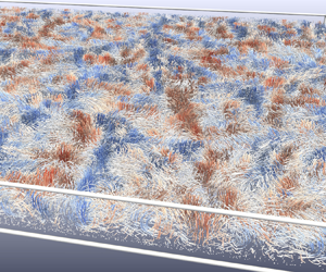
Examples of short tracks are shown in figure 2 for SQR16_1 (figure 2a) and CYL1_3 (figure 2b). The colour-code in these images represent the vertical velocity. The difference in the large-scale flow organisation between these two cases with aspect ratios  $\varGamma =16$ (figure 2a) and $\varGamma =1$ (figure 2b) is clearly visible. The flow in the large aspect ratio cell (figure 2a) exhibits large lateral coherent structures, of positive vertical velocity, due to the warm fluid rising from the bottom. In between these areas the cold fluid sinks to the bottom, with negative velocities marked by blue tracks. We have analysed these Eulerian flow structures in our previous work (Weiss et al. Reference Weiss, Schanz, Erdogdu, Schröder and Bosbach2023). There we found for $ {\textit {Ra}}=1.1\times 10^6$, Pr = 7.0 and $\varGamma =16$ that its periodicity has a wavelength of approximately $\lambda \approx 3H$, hence the width of a single roll is approximately 1.5 $H$. In the vertical direction, the structures cover the entire height.
Visualisation of particle tracks measured in different convection cells. Panel (a) shows tracks of dataset SQR16_1. For better visualisation particle tracks were cut at a midheight to better highlight the horizontal large-scale flow structures. Panel (b) shows tracks of dataset CYL1_3. Image adapted from Godbersen et al. (Reference Godbersen, Bosbach, Schanz and Schröder2021). The colours in both images represent vertical velocities.
The flow organisation in the  $\varGamma =1$ cylinder (figure 2b) is very different. There, it forms one LSC, which extends through the entire cylinder. Warm fluid rises on the right (positive velocities, red) and sinks on the left (negative velocities, blue). In first order, the width and the height of the LSC is close to $H=D$, however, its shape can be elliptical with its long axis diagonally aligned with the cylinder axis. Then, smaller corner rolls occur in the opposite corners.
3. Results
3.1. Vertical velocity profiles and Reynolds number measurement
First, we want to look at vertical velocity profiles. For this, we sort the data based on their  $z$-coordinate into one of 200 equally spaced bins, and calculate conditional averages for each bin. We do this for at least 10 000 time steps within the duration of the measurement of more than 1000 free-fall times. Results for $\varGamma =16$ and three different Ra (datasets SQR16_1, SQR16_2, SQR16_3) are shown in figure 3. Since there is no significant mean flow, we consider the squared velocities and because, further, the two horizontal components ( $u$ and $v$) are statistically similar, we add them together. We show in figure 3(a) the square horizontal velocity normalised by the square of the free-fall velocity $u_{f}=\sqrt {H\alpha g \Delta T}$. Profiles for different Ra look similar. They exhibit two maxima close to the top and the bottom plate and a minimum at midheight ( $z=0.5H$). This is expected for RBC of sufficiently large aspect ratios (say $1\lesssim \varGamma$), where the flow organises into convection rolls of sizes similar to the cell height. Therefore, fluid parcels are mainly transported vertically from the bottom to the top and are deflected there in horizontal direction. As a result of the larger horizontal velocities close to the top and bottom plates, shear boundary layers develop with large vertical gradients.
Comparison of the vertical velocity profile of three different Rayleigh numbers, given in the legends in panel (b), for  $\varGamma =16$. Shown are (a,c) the horizontal kinetic energy and (b,d) the vertical kinetic energy. Panels (a,b) show data normalised by $u_{f}^2$, corresponding to ${\textit {Re}}\propto Ra^{0.5}$. Panels (c,d) show data normalised by $u_{f}^{2.4}$, corresponding to $ {\textit {Re}}\propto Ra^{0.6}$.

Figure 3(b) shows similar plots for the vertical velocity component  $w^2/u_{f}^2$. The vertical velocity reaches its maximum at $z=0.5H$, decreases towards the top and bottom plate and hits the vertical boundaries with a zero gradient. Again, such profiles are typical for RBC flows in containers of sufficiently large aspect ratio and are explained by the largest convection structures that extend from the bottom to the top. We note in this context that the velocity profiles in slender containers show multiple minima and maxima since multiple convection rolls can occur on top of each other (Zwirner, Tilgner & Shishkina Reference Zwirner, Tilgner and Shishkina2020).
When normalised by  $u_{f}^2$, all curves for different Ra are rather close to each other, despite their squared velocities in physical units differing by a factor of two between the largest and the smallest Ra. However, also normalised, the velocities are slightly larger for larger Ra. Furthermore, the maxima of $(u^2+v^2)/u_{f}^2$ are shifted towards the top and bottom walls, resulting in smaller boundary layers with steeper averaged velocity gradients. This effect is rather small in the Ra range considered here, but nevertheless clearly visible in figure 3(a).
While normalising the data by  $u_{f}$ seems like an obvious choice at first glance, since this is the velocity scale which is often used to derive the dimensionless Oberbeck–Boussinesq equations from the momentum and energy equation, there is a priori no theory predicting that the typical velocity actually scales with $u_{f}$. From (1.1) and the definition of $u_{f}$, we see that the Rayleigh number can be written as
 \begin{equation} {\textit{Ra}} = \frac{u_{f}^2H^2}{\nu\kappa}, \end{equation}
and therefore a scaling  $U\propto u_{f}$ would imply $ {\textit {Re}} \propto {\textit {Ra}}^{0.5}$. In fact, while the Grossmann–Lohse (GL) model theoretically predicts various scaling exponents $\beta$ for $ {\textit {Re}}\propto Ra^\beta$ , ranging from $\beta = 2/5$ to $2/3$ (depending on Pr and Ra, (Grossmann & Lohse Reference Grossmann and Lohse2000, Reference Grossmann and Lohse2001; Stevens et al. Reference Stevens, van der Poel, Grossmann and Lohse2013)), experimentally usually exponents $\beta \le 0.5$ have been observed (Sun & Xia Reference Sun and Xia2005; He et al. Reference He, van Gils, Bodenschatz and Ahlers2015). Evaluating $\beta$ from the GL model for $ {\textit {Ra}}=10^6$ and $ {\textit {Pr}}=7$ results in $\beta = 0.47$. We note, however, that the GL model is based on coefficients that are fitted to existing data. At the time of publication of Stevens et al. (Reference Stevens, van der Poel, Grossmann and Lohse2013), no data for small $ {\textit {Ra}}<10^8$ at $ {\textit {Pr}} >1$ were available and therefore the GL model is less reliable for this parameter range.
In an attempt to find a better collapse of the data for different Ra, we varied the exponent  $\gamma$ that was used to normalise the data in figure 3(a,b), i.e. $u_f^\gamma$, and tried to minimise the difference between the velocity profiles of the largest ( $ {\textit {Ra}}=2.4\times 10^6$) and the smallest Rayleigh number ( $ {\textit {Ra}}=1.1\times 10^6$). The smallest difference, and hence the best collapse is achieved with $\gamma =2.4$. Therefore, we normalise the squared velocity by $u_{f}^{2.4}$ and show the result in figure 3(c,d). Note that we also have to multiply by $(\nu /H)^{0.4}$ in order to have non-dimensional values. The data normalised in this way show a much better collapse for all three Ra, in particular for the vertical velocity component. We want to stress that a perfect collapse is not expected since the velocity profiles of course do depend on Ra. Solely for the averaged velocity $U$ are scaling relations with Ra and Pr predicted. Anyhow, the fact that a normalisation by $u_{f}^{2.4}$ brings data for different Ra close to each other strongly suggests a relation $ {\textit {Re}}\propto {\textit {Ra}}^{0.6}$ with an exponent that is somehow larger than what has been found by other experimental studies (Sun & Xia Reference Sun and Xia2005; He et al. Reference He, van Gils, Bodenschatz and Ahlers2015). However, these studies were conducted at slightly larger Ra. There are DNS results by Shishkina et al. (Reference Shishkina, Emran, Grossmann and Lohse2017) available, who have calculated Re for a large variety of Ra and Pr, also for parameters similar to ours. They find that for $ {\textit {Pr}} =5$ and similarly $ {\textit {Pr}} =10$ (magenta and cyan squares in figure 2d of Shishkina et al. (Reference Shishkina, Emran, Grossmann and Lohse2017)) the exponent $\beta$ decreases from $\beta =2/3$ at $ {\textit {Ra}} = 10^5$ to $\beta < 1/2$ at $ {\textit {Ra}} = 10^9$. Visual inspection of figure 2(d) in Shishkina et al. (Reference Shishkina, Emran, Grossmann and Lohse2017) shows $\beta \approx 0.6$ at $ {\textit {Ra}} = 10^6$, which is in good agreement with our observation here.
Figure 4 compares vertical velocity profiles for three datasets with very different  $\varGamma$, Ra and Pr. Because Ra and Pr vary significantly, the exponent $\beta$ is not expected to be constant, but will rather change between $0.45\lesssim \beta \lesssim 0.6$ in the Ra range investigated according to Stevens et al. (Reference Stevens, van der Poel, Grossmann and Lohse2013) and Shishkina et al. (Reference Shishkina, Emran, Grossmann and Lohse2017). Therefore, we assume $\beta =0.5$ and normalise our data by $u_{f}^2$. By doing so we have accounted only for the Ra-dependency, but have not yet taken into consideration that also Pr varies by a factor of 10 between the different datasets. In order to also account for the different Pr, we look again in the paper by Shishkina et al. (Reference Shishkina, Emran, Grossmann and Lohse2017), and find a scaling relation of something close to $ {\textit {Re}}\propto {\textit {Pr}}^{-0.8}$ for the parameter ranges of our datasets (the exponent in fact changes slightly with Ra). With this we write
 \begin{equation} U=\frac{{\textit{Re}} \nu}{H}\propto \frac{\nu}{H} Ra^{0.5}{\textit{Pr}}^{{-}0.8} = u_{f} \left(\frac{\nu}{\kappa}\right)^{1/2}{\textit{Pr}}^{{-}0.8}=u_{f}{\textit{Pr}}^{{-}0.3}. \end{equation}
Therefore, we normalise the squared velocities in figure 4 by  $u_{f}^2 {\textit {Pr}}^{-0.6}$. With this scaling the magnitude of the squared velocities are rather similar, despite having different Ra by up to three orders of magnitude. As has been found already above, with increasing Ra the maxima of $(u^2+v^2)/u^2_{f}$ move close to the top and bottom plate, hence reducing the size of the kinetic boundary layers there. Furthermore, the minimum seems to become flatter with increasing Ra, and less deep compared with the maxima close to the top and bottom. Similarly, also the maxima of $w^2/u^2_{f}$ become broader and the slope close to the top and bottom boundaries becomes steeper.
Comparison of the vertical velocity profile for three different aspect ratios and  $Ra$. Shown are (a) the horizontal and (b) the vertical kinetic energy normalised by $u^2_{f} {\textit {Pr}}^{-0.6}$. The different lines correspond to the different data sets as labelled in table 1: solid blue, $\varGamma =16$, $ {\textit {Ra}} = 1.1\times 10^6$, Pr = 7.0; dashed red, $\varGamma =8$, $ {\textit {Ra}}=9.1\times 10^6$, Pr = 7.0; solid yellow, $\varGamma =1$, $ {\textit {Ra}}=1.5\times 10^9$, $ {\textit {Pr}}=0.7$.

Even though all relevant control parameters (e.g. Ra, Pr,  $\varGamma$) are different for the three datasets, we note that certain aspects of the profiles can be explained by the influence of Ra and Pr alone. For instance we know that the thickness of the kinetic boundary layers at the top and bottom scales similar to a Prandtl–Blasius boundary layer (see e.g. Ching et al. Reference Ching, Leung, Zwirner and Shishkina2019), i.e. they become thinner with increasing Ra and decreasing Pr, according to
 \begin{equation} \frac{\delta}{H} \propto {\textit{Re}}^{{-}1/2} \propto {\textit{Ra}}^{{-}1/4} {\textit{Pr}}^{0.4}. \end{equation}
This explains the very thin boundary layers for  $ {\textit {Ra}} = 1.6\times 10^9$ (dataset CYL1_3). Also, with increasing turbulence intensity the velocity profile at midheight is expected to become flatter and the minimum in the horizontal velocity (figure 4) to become higher, relative to the maxima because the turbulence intensity increases in the bulk.
The influence of  $\varGamma$ on the vertical profiles is expected to be small at least for $\varGamma =16$ and $\varGamma =8$. In fact for sufficiently large $\varGamma$, the influence of the sidewall becomes negligible. This is certainly the case for $16\lesssim \varGamma$, as it has been shown in DNS that the Eulerian integral length scale saturates around these aspect ratios (Stevens et al. Reference Stevens, Blass, Zhu, Verzicco and Lohse2018). However, when considering only averaged horizontal or vertical velocities, their value already saturates close to $\varGamma \approx 4$ or so (Stevens et al. Reference Stevens, Blass, Zhu, Verzicco and Lohse2018).
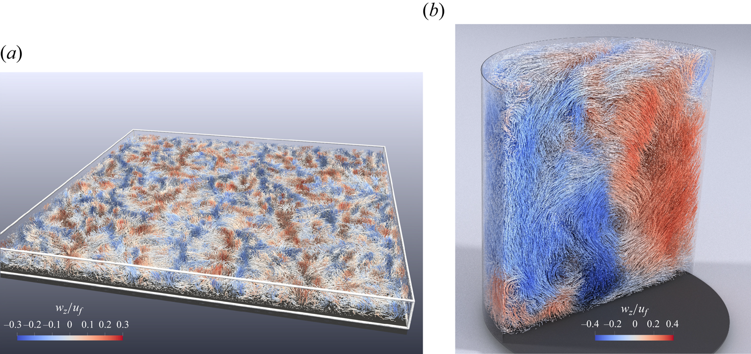
Since we have velocity data for the entire fluid volume, we can also calculate volume-averaged Re and see how it depends on Ra and Pr. While the number of different data points and the Pr and Ra range they cover is not sufficient for a thorough exploration, we still can test whether they agree with DNS studies by Shishkina et al. (Reference Shishkina, Emran, Grossmann and Lohse2017). For this, we plot in figure 5(a) the Pr-normalised Reynolds number ( $ {\textit {Re}} {\textit {Pr}}^{0.8}$) as a function of Ra for our data (solid) and compare them with results from DNS that were acquired in cylindrical RBC cells with $\varGamma =1$. We see that in this presentation the data for very different $ {\textit {Pr}}$, i.e. $ {\textit {Pr}}=0.7$ (blue circles) and $ {\textit {Pr}}=7.0$ (orange squares and triangles), rather decently fall onto a power law curve $\propto {\textit {Ra}}^{1/2}$ (black line). Figure 5(b) shows the same data but now also normalised by $ {\textit {Ra}}^{1/2}$ and plotted along a linearly scaled $y$-axis. Let us first consider the experimental data, i.e. the solid symbols. Plotted in this way, the data are rather close to each other over more than three orders of magnitude in Ra. While being close, they are not identical and differ by up to 30 %. This is not surprising since there is not a single scaling relation between Re, Pr and Ra that holds for the entire Pr and Ra range covered here. We see that both the orange squares for $\varGamma =16$ as well as the orange triangles for $\varGamma =8$, increase with increasing Ra, since for them Re depends on Ra with a larger exponent than 0.5, while the blue bullets are somehow lower, because in this case the exponent is smaller.
Reynolds number as a function of Ra. (a) Reynolds number normalised by  $ {\textit {Pr}}^{-0.8}$ shows a power law trend as a function of Ra on a log–log plot. The black line is $0.16 {\textit {Ra}}^{1/2}$. (b) The same data normalised also by $ {\textit {Ra}}^{1/2}$ on a semi-logarithmic plot. Solid symbols mark data from this experiments; open symbols mark DNS results from Shishkina et al. (Reference Shishkina, Emran, Grossmann and Lohse2017). Different colours mark different Pr and different symbols mark different $\varGamma$ according to the legend. All DNS results were calculated in cylindrical cells with $\varGamma =1$. Control parameters for each data point are given in the legend. The error bars mark the uncertainty in the measurement of the temperature difference due to the thermal boundary layer on top of the top plate of $s_{\Delta T} =0.2$ K.
We also note that one orange triangle ( $\varGamma =8$) at $ {\textit {Ra}}=1.6\times 10^6$ is significantly smaller than the orange square ( $\varGamma =16$) at the same Ra. We believe that this discrepancy is due to measurement uncertainties of $\Delta T$, which become important here, since this data point was taken at $\Delta T=1.85$ K and the uncertainty of the measurement of $\Delta T$ and hence Ra, becomes large. While we can measure the temperature of the bottom plate rather precisely, the temperature at the top plate is estimated from measurements of the cooling water. We do correct the measurements by taking the temperature drop across the top plate into consideration, but we do not correct for thermal boundary layers that occur atop the top plate in the cooling water. Therefore, it is possible that we have overestimated $\Delta T$ and Ra. Assuming an uncertainty of $s_{\Delta T} =0.2$ K, we have plotted error bars in the $y$ direction to the data points. In most cases the error bars are small compared with the symbol size, but the error bar for this particular point reaches up to the orange square ( $\varGamma =16$) at the same Ra.
We have also plotted in figure 5 with open symbols results from DNS for different Pr. They overall agree fairly well with our data in the following manner. After normalising the data by  $ {\textit {Ra}}^{1/2}$ (in figure 5b) the experimental data for $ {\textit {Pr}}=7.0$ (orange squares and orange triangles) as well as the DNS data for $ {\textit {Pr}}=5$ (green open circles) and $ {\textit {Pr}}=10$ (brown open circles), both increase with increasing Ra. However, their absolute values are significantly smaller than our experimental points, which we attribute to the much smaller aspect ratio of $\varGamma =1$. Shear forces at the sidewalls are expected to slow down the flow in particular at large Pr and small Ra. We further see that this discrepancy is much smaller for $ {\textit {Pr}}=0.7$ (blue open circles and blue bullets). Here, both DNS and experiment were conducted in $\varGamma =1$ cylinders and albeit the DNS data are only available until $ {\textit {Ra}}=10^7$, their Ra trend is rather flat and an extrapolation to $ {\textit {Ra}}=10^9$ seems to agree well with our measured data.
3.2. Energy dissipation rate
In 3-D HIT the kinetic energy dissipation rate  $\varepsilon$ describes the transfer of energy from large to small scales. It is probably the most relevant quantity there as it determines many relevant statistical flow properties in the inertial range. Although $\varepsilon$ is not a Lagrangian property (we calculated it from the FlowFit-generated Eulerian field) and as such does not really fit the scope of this paper, we will nevertheless discuss it quickly here since we need its global average to estimate Kolmogorov length and time scales. Furthermore, calculating $\varepsilon$ is useful to test the quality of our data.
We have mentioned already above (1.5) that  $\varepsilon$ can be calculated from Ra, Pr, Nu and $\nu$. Our experiments were designed for high-precision velocity measurements and not for heat flux measurements. Even though we did measure the heating power of the bottom plate, there is a parasitic heat flux through the sidewalls which were not insulated. As a result, we could measure $ {\textit {Nu}}$ only with an uncertainty of approximately 7 % (for SQR) and 10 % (for CYL). Therefore, we estimated for the CYL1 set-up, $ {\textit {Nu}}$ from Ra, and Pr, based on the GL theory (Stevens et al. Reference Stevens, van der Poel, Grossmann and Lohse2013). In this parameter range GL is quite accurate and agrees well with experiments and DNS.
For the rectangular cell filled with water (SQR16 and SQR8) the particle concentrations are high enough to resolve even the smallest scales in the flow. Therefore, we used FlowFit (Gesemann et al. Reference Gesemann, Huhn, Schanz and Schröder2016) to calculate the Eulerian velocity field and the velocity gradient tensor  $S_{ij}=\frac {1}{2}(\partial _i u_j + \partial _j u_i)$. This allowed us to calculate directly the energy dissipation rate
 \begin{equation} \varepsilon = 2\nu \langle S_{ij}S_{ji}\rangle. \end{equation}
For the readers’ convenience, we show in figure 6 vertical profiles of the horizontally and temporally averaged kinetic dissipation rates from two different datasets, in which Ra differs by a factor of eight. In these profiles one again sees clearly the boundary layers at the top and bottom with high shear rates and hence high rates of energy dissipation, whereas in the bulk the dissipation is much smaller. We also see very clearly that with increasing Ra the boundary layers become thinner. As a result, even though the shear rate and hence the energy dissipation rate inside the boundary layers increases with Ra, their relative contribution to the total dissipation rate decreases. Most of the energy dissipation takes place in the bulk in large Ra convection.
Normalised kinetic energy dissipation as a function of the vertical coordinate for the datasets SQR16_1 (blue bullets,  $ {\textit {Ra}}=1.1\times 10^6$, $\varGamma =16$) and SQR8_2 (red squares, $ {\textit {Ra}}=9.1\times 10^6$, $\varGamma =8$). Note that the energy dissipation is normalised by their mean values in order to better compare the different datasets.

In table 2 we provide values for  $\varepsilon$, the Kolmogorov length $\eta _k$, the Kolmogorov time $\tau _\eta$, as well as the kinematic viscosity. For SQR we provide $\varepsilon$ based on (1.5) and (3.4). For the former Nu was measured based on the heat input into the bottom plate.
Energy dissipation rates and Kolmogorov microscales for the datasets. Values in blue were used for calculating  $\eta _k$ and $\tau _\eta$.

3.3. Velocity autocorrelation
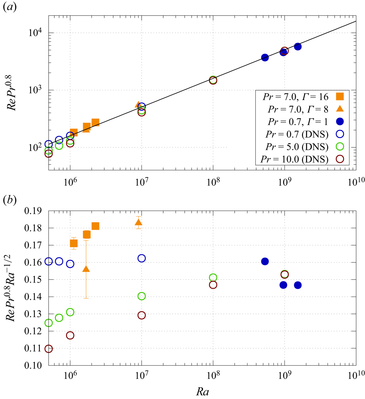
Due to their chaotic nature, turbulent flows are only correlated over finite times and lengths, and hence typical correlation length and times are characteristic features of a given flow and reflect its degree of turbulence. In order to characterise our flow, we calculate the normalised autocorrelation function of the velocity of a given particle as
 \begin{equation} C_{uu}= \frac{ \langle u(t)u(t+\tau)\rangle_{t,p} }{\langle u^2 \rangle_{t,p}}, \end{equation}
with  $u$ representing one of the velocity components and the average is taken over all available tracks of sufficient length (at least 100 time steps). Results are shown in figure 7 for three datasets of different $\varGamma, {\textit {Ra}}$ and Pr (see legend). Note again that time is scaled with the corresponding free-fall time of each dataset and therefore the decay occurs over the same magnitude of times. While we do not show corresponding data, we would like to stress that there are qualitative differences for the autocorrelation function of the two horizontal components $u$ and $v$. The system is not fully symmetric because the large-scale turbulent super structures show a preferential alignment for $\varGamma = 8$ and 16 and also the LSC for the $\varGamma =1$ case has a mean orientation. For example, large-scale structures elongated in the $x$ direction would lead to fluctuations mostly visible in $C_{vv}$ but not so much in $C_{uu}$. This dominant orientation did not average out within our measurement duration. Therefore, we show in figure 7(a,b) the mean autocorrelation of the two horizontal components, i.e. $(C_{uu}(\tau )+C_{vv}(\tau ) ) /2$ and in figure 7(c,d) the autocorrelation of the vertical component ( $C_{ww}$).
Averaged velocity autocorrelation of the two horizontal components (a,b) and the vertical component (c,d) for three different aspect ratios and Ra; datasets SQR16_1, SQR8_2, CYL1_3, see legend in (a). The coloured lines in (b,d) are parabolic fits of (3.6) to the data for very small  $\tau$. The fit parameters $\tau _{TA}$ are provided in the legends. The black lines in (c) are fits of (3.6) to the data. The fit parameter are provided in the legend.
Let us first look at the  $(C_{uu}+C_{vv})/2$ as shown in figure 7(a). All three curves decay initially rather fast, as is expected for turbulent flows. However, in contrast to isotropic turbulence, they also reach negative values and after reaching a minimum $(C_{uu}+C_{vv})/2$ increase again. In particular for data from the cylinder ( $\varGamma =1$, yellow triangles) three oscillation cycles are clearly visible before $(C_{uu}+C_{ww})/2$ asymptotically reaches zero. These oscillations are less pronounced, but still clearly visible in the data for $\varGamma =16$ (blue bullets) and $\varGamma =8$ (red squares). They are caused by the quasiperiodic motion of the particles within the coherent structures, which transports the particles from the bottom to the top where they are deflected in the horizontal direction before they sink back to the bottom.
Because in the  $\varGamma =1$ cylinder the flow is organised into one LSC, the tracer particles are following quasiperiodic trajectories which fully decorrelate only after times significantly longer than one such turnover time. Particles which are transported along one sidewall from the bottom to the top can only move along the top plate towards the opposite side where they sink back to the bottom.
The horizontal periodicity of this motion is significantly weaker for particles in the square cells of  $\varGamma =16$ and 8. There, particles also move up and down quasiperiodically, causing long correlations for the vertical velocity $C_{ww}$. However, particles that were transported from the bottom to the top are not so much confined by the sidewalls and therefore can in principle move in any horizontal direction. Only the existence of large turbulent roll-like superstructures can force the particles to move along elliptical paths causing a weak quasiperiodicity in $(C_{uu}+C_{vv})/2$, but only for a rather short time comparable to an eddy-turnover time of the largest scales. Note in this regard that the first minimum in $(C_{uu}+C_{vv})/2$ is deeper for $\varGamma =16$ than for $\varGamma =8$. This is because the large lateral convection structures in $\varGamma =16$ are more coherent than for $\varGamma = 8$.
If we want to determine a typical eddy-turnover time  $T_{to}$, we better look at the vertical component $C_{ww}$, where oscillations are stronger and clearly visible. In fact we can determine $T_{to}$ as well as a typical time scale over which correlation is lost $\tau _{co}$ by fitting the following function to the data:
 \begin{equation} y(\tau) = \exp{(-\tau/\tau_{co})}\cos{((\tau+\tau_0) 2{\rm \pi}/T_{to})}. \end{equation}
The fitted functions are included as black lines in figure 7(c) and the fitted parameters  $\tau _{co}$ and $T_{to}$ are provided in the legend.
We have also allowed a small phase shift  $\tau _0$ inside the cosine function that was also used as a fit parameter. While we cannot provide a physical interpretation of $\tau _0$, we note that its positive value means that the first minimum occurs at $\tau$ that are smaller than half the period $T_{to}$. One could speculate that this is because most particles move in eddies that are smaller than the coherent superstructures. However, on longer time scales ( $\tau$) only the period of the largest time scale ( $T_{to}$) is visible because all smaller eddies average out.
We see that the red ( $\varGamma =8$) and blue ( $\varGamma =16$) data are very close to each other, whereas the yellow ( $\varGamma =1$) are different. For a better scaling, a factor $ {\textit {Pr}}^{-0.3}$ needs to be included in $\tau$, which brings in particular the first minimum of the yellow triangles closer to the minima of the red squares and blue bullets. For comparison we provide Pr-corrected time scales in table 3. We see that after correcting, the eddy-turnover times $T_{to} {\textit {Pr}}^{-0.3}$ and also the coherence time $\tau _{co} {\textit {Pr}}^{-0.3}$ are rather similar for all three investigated datasets despite their vastly different Ra, by three orders of magnitude. This is again evidence that the typical velocities in RBC roughly scale as $ {\textit {Re}}\propto {\textit {Ra}}^{1/2} {\textit {Pr}}^{-0.8}$ (neglecting variations in the different Ra, and Pr, regimes).
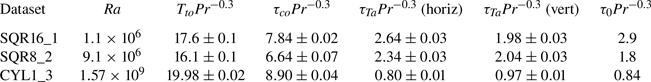
From figure 7 and table 3 we see that  $\tau _{co} < T_{to}$ for all datasets, whereas both seem to be universal after being compensated by $ {\textit {Pr}}^{-0.3}$. This means that correlation has already decreased significantly before a particle has made one round, e.g. from the bottom to the top and back. This can be compared to measurements in HIT, where the largest eddies are less coherent than here (Sato & Yamamoto Reference Sato and Yamamoto1987; Pope Reference Pope2000) and velocity correlation does not exhibit oscillations, but can be well represented by a pure exponential decay of $C_{uu}(\tau )$. The Lagrangian integral time scale is then defined as $T_0\equiv \int _0^\infty C_{uu}\,{\rm d}\tau$ and it is believed to be proportional to the Eulerian integral times scale (Corrsin Reference Corrsin1963). Although RBC is neither homogeneous nor isotropic and therefore quantities such a correlation functions or Lagrangian integral time scales depend on the initial location of the particles considered, results from spatially averaged statistics as done here are nevertheless very useful and exhibit some universality, as we will show below. Nevertheless, we provide a spatially resolved analysis in the Supplemental material.
On a very short time scale, the velocities are still strongly correlated for durations of the order of an eddy turnover corresponding to flow structures that are so small that viscous dissipation already plays a role. To shine some light on these processes, we fit a parabolic function
 \begin{equation} y(\tau) = 1 - \left(\frac{\tau}{\tau_{Ta}}\right)^2 \end{equation}
to the data for very small  $\tau$. Herewith, the time scale $\tau _{Ta}$ is the Lagrangian analogue to the Taylor-microscale in the Eulerian view (Pope Reference Pope2000). The values for $\tau _{Ta}$ are shown in the legends of figure 7(b,d) and Pr-corrected values $\tau _{Ta} {\textit {Pr}}^{-0.3}$ are provided in table 3. One would expect that $\tau _{Ta} {\textit {Pr}}^{-0.3}$ decreases with increasing turbulence, or in our case with increasing Ra. While we do observe the smallest $\tau _{Ta} {\textit {Pr}}^{-0.3}$ for the largest Ra, ( $1.57\times 10^9$), for $ {\textit {Ra}}=1.1\times 10^6$ and $ {\textit {Ra}}=9.1\times 10^6$ the results are much less clear. While for the horizontal component $\tau _{Ta} {\textit {Pr}}^{-0.3}$ is indeed longer for the smaller Ra, for the vertical component they are, within their uncertainties, the same.
3.4. Particle displacement
One fundamental property of turbulent flows is their ability to transport material, such as for instance solutes or aerosols. To investigate and quantify such transport processes it is common to look how fast fluid tracers are displaced in time by the turbulent flow. In order to do this we calculated the average particle displacement for a given time period  $\tau$ as
 \begin{equation} \varDelta_i^2 (\tau) = \langle (x_i(t + \tau) - x_i(t))^2 \rangle_{t,p}, \end{equation}
with the average  $\langle \rangle$ taken over time $t$ and also over many particles ( $p$). Since in RBC the vertical direction is fundamentally different from the horizontal directions, we consider each component separately.
Figure 8(a) compares the displacements in all three directions for the dataset SQR16_1. In this figure, the displacement is expressed in units of the cell height  $H$ and the time was normalised by the free-fall time $t_{f}$. The curves for $\varDelta _x^2$ and $\varDelta _y^2$ are very similar and in particular show two distinct regimes. For small $\tau$ the data exhibit a ballistic behaviour with $\varDelta _{x,y}^2 \propto \tau ^2$, while for larger $\tau$ they follow a diffusive behaviour with $\varDelta _{x,y}^2\propto \tau$. In general, diffusive displacement occurs when particles move chaotically and uncorrelated on the considered time scales. Therefore, it is no surprise to see that the transition from the ballistic to the diffusive regime in our data occurs close to the typical correlation time $\tau /t_f \approx \tau _{co}$ (black vertical line in figure 8), which we have determined from analysing the velocity autocorrelation in the previous section.
(a) Spatial displacement in the  $x$ direction ( $\varDelta _x^2$, blue circles), the $y$ direction ( $\varDelta _y^2$, red squares) and the $z$ direction ( $\varDelta _z^2$, green diamonds) as a function of time duration for $ {\textit {Ra}}=1.1\times 10^6$ (SQR16_1). The green and yellow line mark a quadratic and a linear function. (b) $\varDelta _x^2$ as a function of time for three different Ra, (see legend) (SQR16_1, SQR16_2, SQR16_3). All data are for $ {\textit {Pr}}=7.0$ and $\varGamma =16$. The vertical black lines mark $\tau _{co}=7.8 {\textit {Pr}}^{0.3}$ as calculated from fits to the autocorrelation function (see table 3). The horizontal black lines marks $\varDelta _{z,\infty }^2=0.167$, i.e. the displacement of a random walker in the confined enclosure ( $z_i\in \{0,1\}$).

The vertical displacement  $\varDelta _z^2$ (green diamonds in figure 8) also shows a ballistic regime with the same slope as the other two components, hence the system appears isotropic on small scales, despite the presence of buoyancy in the $z$ direction. However, $\varDelta _z^2$ does not show a diffusive regime on longer time scales. In fact, the curve reaches a maximum at around $\tau /t_f\approx \tau _{co}$, decreases again and after a few decaying oscillations settles close to $\varDelta _z^2(\infty )\approx 0.17$. This behaviour is due to the vertical confinement of the cell and $\varDelta _z^2(\infty )$ can be calculated as the mean square difference between randomly placed particles in the range from $z_{i,j}\in \{0,1\}$, i.e.
 \begin{equation} \varDelta^2_z(\infty) = \frac{1}{N(N-1)}\sum_{i\not = j}(z_i-z_j )^2 = 0.167. \end{equation}
The initial overshoot and the subsequent decaying oscillations can be explained by the fact that the vertical dimension of the coherent structure is as large as the cell height. Therefore, a particle that is initially close to the bottom is usually transported first into the upper half of the cell close to the top plate, and then back to the bottom. The time at which  $\varDelta _z^2$ reaches its maximum is therefore related to the eddy-turnover time $T_{to}$. The fact that a few (damped) oscillations are visible indicates that correlation of the velocity is not entirely lost after a particle has been stirred around once throughout the entire cell, a fact already seen in figure 7. We also see that the time at which the maximum is reached for $\varDelta _z^2$ is also the time at which the diffusive regime starts for $\varDelta _x^2$ and $\varDelta _y^2$ and where most of the correlation in horizontal direction is lost, i.e. $\tau /t_f\approx \tau _{co}$. Quadratic and linear fits to the data here reveal squared velocities in the ballistic regime of $9.2\times 10^{-3}u_{f}^2$ as well as a diffusion constant of $0.05H^2/t_{f}$.
We also compare in figure 8(b) the displacement for different Ra at the same  $ {\textit {Pr}} = 7.0$ and $\varGamma =16$. For simplicity we only show $\varDelta _x^2$. The data plotted in this way all collapse on the same curves. While this is at a first glance rather surprising since the thermal driving changes by a factor of two, this observation can easily be explained. If we remember the findings shown in figure 3, namely that the velocities in the flow scale with the free-fall velocity $u_{f}$ as Ra is changed, the slope $\varDelta _i^2/\tau ^2$ in the ballistic regime is nothing other than the averaged square velocity. And since $\varDelta _i^2$ is normalised by $H^2$ and $\tau$ is normalised by $t_{f}$, this coefficient is already normalised by $u_{f}=H/t_{f}$ and therefore should not change anymore with Ra.
From figure 8(a) we see that the transition to the diffusive regime occurs close to  $\tau /t_f\approx \tau _{co}$, i.e. when most of the correlation is lost, which is rather independent of Ra (in dimensionless units). Therefore, also the diffusion constant should be independent of Ra as long as displacement and time are scaled properly. We acknowledge that this fact is against our intuition, which suggests that stronger thermal driving should enhance turbulent diffusion. But the independence on Ra observed here is only the case in dimensionless units, whereas in physical units the diffusion is indeed enhanced and proportional to Ra.
In figure 9 we compare the displacement also for different  $\varGamma, {\textit {Ra}}$ and Pr, namely for the datasets SQR16_1 (blue, $\varGamma =16$), SQR8_2 (red, $\varGamma =8$) and CYL1_3 (yellow, $\varGamma =1$). In order to account for the different Pr of these datasets, we multiply the time by $ {\textit {Pr}}^{-0.3}$. The horizontal displacement $(\varDelta _x^2+\varDelta _y^2)/H^2$ (figure 9a) shows a collapse of the data in the ballistic regime, despite their differences in $ {\textit {Ra}}, {\textit {Pr}}$ and $\varGamma$. In the diffusive regime, for larger $\tau$, only the data for $\varGamma =8$ (red open squares) and $\varGamma =16$ (blue circles) collapse, whereas the data for $\varGamma =1$ (yellow triangles) flatten and become independent of $\tau$. This suggests that for sufficiently large $\varGamma$, the width of the coherent structures in the flow is determined by the cell height $H$ and not by its lateral extent $H\varGamma$.
(a) Horizontal displacement  $\varDelta ^2_x+\varDelta ^2_y$ for different $\varGamma$, $ {\textit {Ra}}$ and Pr, (see legend) as a function of time duration, which is normalised to account for the different Pr. The yellow, red and blue horizontal dashed lines are the expected saturation values for the cell with $\varGamma = 1$ ( $\varDelta ^2_{h,\infty }=0.25$), $\varGamma =8$ ( $\varDelta ^2_{h,\infty } =21.3$), $\varGamma =16$ ( $\varDelta ^2_{h,\infty }=85.3$). (b) Vertical component $\varDelta ^2_z$ for the same data. The horizontal line marks $\varDelta ^2_{z,\infty }=1.667$. The black vertical lines in both plots mark $(\tau /t_f) {\textit {Pr}}^{-0.3} = 8\approx \tau _{co} {\textit {Pr}}^{-0.3}$.

The flattening of the  $\varGamma =1$ data is due to the finite size of the container, hence very similar to the vertical component $\varDelta ^2_z$ for $\varGamma =16$ (shown in figure 8a). Also here, the displacement after a very long time, is time-independent and is given by the mean squared distance of the all particles, i.e.
 \begin{equation} \varDelta^2_{h,\infty} \equiv\varDelta^2_{x}(\infty)+\varDelta^2_y(\infty) = \frac{1}{N(N-1)}\sum_{i\not = j}[(x_i-x_j )^2 + (y_i - y_j)^2]. \end{equation}
We note that the exact values of  $\varDelta ^2_{h,\infty }$ do depend on the actual shape of the container and not just on its aspect ratio. We show in figure 9(a) $\varDelta ^2_{h,\infty }$ as horizontal lines for each of the set-ups. One sees, that the yellow triangles (CYL1_3) settle for very large $\tau /t_{f}$ exactly on that line for $\varDelta _{h,\infty }^2$.
We also show horizontal lines marking  $\varDelta ^2_{h,\infty }$ for the other two datasets with $\varGamma =8$ (red) and $\varGamma =16$ (blue). The slope of the data for $\varGamma = 8$ also clearly decreases for very large $\tau$ when $\varDelta ^2$ becomes close to $\varDelta ^2_{h,\infty }$ hence, also here the displacement is bound by the size of the cuboid cell. Particle tracks for the measurements of the largest aspect ratio ( $\varGamma =16$, blue) are not long enough to reach $\varDelta ^2_{h,\infty }$. In fact, from the diffusive behaviour one could estimate that $\varDelta ^2_{h,\infty }$ would have been reached at $1700\,t_{f}$ which is longer than the duration of the experiment.
Figure 9(b) shows a comparison of the vertical displacement  $\varDelta ^2_z$ of the same three data sets. The vertical confinement is now visible in all data sets and is dominant at time lags of around $(\tau /t_f) {\textit {Pr}}^{-0.3}>\tau _{co} {\textit {Pr}}^{-0.3}$, as indicated by the black vertical line. For smaller $\tau /t_f$, all data overlap and follow $\propto \tau ^2$. Please note again that the data shown here were acquired at very different control parameters. Hence, it seems that their behaviour is universal. Further, as long as $\varGamma$ is sufficiently large, the horizontal displacement follows ${\propto }\,\tau ^2$ for $\tau /t_f< \tau _{co}$) and ${\propto }\,\tau$ for $\tau /t_f> \tau _{co}$, with $\tau _{co} {\textit {Pr}}^{-0.3}\approx 8$, which is the time scale over which correlation is mostly lost.
3.5. The Lagrangian velocity structure function
Many predictions about turbulence assume isotropic and homogeneous conditions (i.e. HIT), which are not met in most real turbulent flows in nature and industry. There, large-scale mean flows exists, which align the orientation of eddies. Nevertheless, theoretical predictions might still be applicable on a local level, i.e. for the fluctuations after a mean flow contribution has been subtracted (Monin & Yaglom Reference Monin and Yaglom1975).
For example, instead of (3.8) the following equation can be considered for particle displacement, which removes the contribution of the mean flow:
 \begin{equation} \varDelta_{c,i}^2 (\tau) = \langle [x_i(t+\tau)- x_i(t) - u_i(t)\tau ]^2 \rangle_{t,p}. \end{equation}
Here  $\varDelta _{c,i}^2$ is now not anymore the particle displacement but rather the relative displacement of the particle compared with a position it would have if the velocity had stayed constant at time $t$. It can be shown (see Supplemental material) that $\varDelta _{c,i}^2$ can be written as
 \begin{equation} \varDelta_{c,i}^2 (\tau) = \frac{1}{2}\int_0^\tau {\rm d} t^\prime \int_0^\tau {\rm d} t^{\prime\prime}[S^2(t^\prime) + S^2(t^{\prime\prime}) -S^2(|t^\prime-t^{\prime \prime}|)], \end{equation}
with  $S_i^2$ being the second-order Lagrangian velocity structure function
 \begin{equation} S_{i}^2(\tau)=\langle [u_i(t+\tau)-u_i(t)]^2\rangle_t. \end{equation} $S_i^2$ is most often considered in theoretical and experimental studies since mean flow effects are already accounted for and because theoretical predictions exist for HIT. That is why here, we present data and discussion for $S_i^2(\tau )$, whereas a similar analysis for $\varDelta _{c,i}^2(\tau )$ is provided in the Supplemental material.
From Kolmogorov's similarity hypothesis and assuming simple scaling relations one can deduce for very turbulent flows three different scaling relations for different durations  $\tau$ (Monin & Yaglom Reference Monin and Yaglom1975),
 $$\begin{gather} S_i^2(\tau) = a_0\varepsilon^{3/2}\nu^{{-}1/2}\tau^2 \quad \mbox{for}\ \tau \ll\tau_\eta, \end{gather}$$
 $$\begin{gather}S_i^2(\tau) = C_0 \varepsilon \tau \quad \mbox{for}\ \tau_\eta\ll \tau \ll T_0, \end{gather}$$
 $$\begin{gather}S_i^2(\tau) = 2\langle u_i^2\rangle \quad \mbox{for}\ T_0\ll \tau. \end{gather}$$
Here,  $\varepsilon$ is the averaged kinetic dissipation rate, $a_0$ and $C_0$ are constants (assumed to be universal for HIT), $\tau _\eta = \sqrt {\nu /\varepsilon }$ is the Kolmogorov time scale and $T_0$ the Lagrangian integral time. As can be seen the velocities in turbulence behave similar to the displacement for a Langevin particle. That is, $S_i^2$ behaves ballistically ( ${\propto }\,\tau ^2$) in the viscous regime (for $\tau \ll \tau _\eta$) and diffusively ( ${\propto }\,\tau$) in the inertial regime ( $\tau _\eta \ll \tau \ll T_0$).
We calculate  $S_i^2(\tau )$ for the datasets SQR16_1 and CYL1_3 and present the results in figure 10. Let us first have a look at the less turbulent case (SQR16_1) in figure 10(a), where we compensate the time lag by $ {\textit {Pr}}^{-0.3}$ to better compare results for different Pr (figure 10c). We note that the structure function for the vertical component $S_w^2$ is slightly above the two horizontal components which we believe is due to the faster velocity changes close to the top and bottom boundaries. Otherwise all three quantities are in principle very similar. In particular they follow at small time lags $\tau$ indeed a power law $S^2 \propto \tau ^2$ which suggests that on these short time scales viscous dissipation is a governing factor.
(a,c) Second-order velocity structure function normalised by the free-fall velocity  $u_f^2$ and plotted against $\tau /t_f$ with $t_f$ being the free-fall time. The black vertical line mark $(\tau /t_f) {\textit {Pr}}^{-0.3}=8\approx \tau _{co} {\textit {Pr}}^{-0.3}$ as a guide to the eye. The coloured horizontal dashed lines mark $\langle u_i^2 \rangle$. The other solid lines mark power laws of various exponents (see corresponding labels). (b,d) The same data but now rescaled by $\tau ^{-3/4}$ and plotted against $\tau /\tau _\eta$. (a,b) Data set SQR16_1 with $ {\textit {Ra}}=1.1\times 10^6$, $\varGamma =16$, $ {\textit {Pr}}=7.0$. (c,d) Data set CYL1_3 with $ {\textit {Ra}}=1.5\times 10^9$, $\varGamma =1$ and $ {\textit {Pr}}=0.7$. Different colours mark the different components (see legend).

The slope decreases for larger  $\tau$ and asymptotically reaches $S_i^2\rightarrow \langle u_i^2\rangle$. The transition to the regime with constant $S_i^2$ happens at $\tau =\tau _{co} {\textit {Pr}}^{-0.3}\approx 8$, i.e. at the same $\tau$ where most correlation is lost and the displacement in figure 8 turns from a ballistic into a diffusive regime. While the data show a continuous change in the slope prior to this point, a clear inertial range with $S_i^2\propto \tau$ as in (3.15) is not visible. This might be due to insufficient separation of scales. Therefore, we show in figure 10(c) data from the much more turbulent dataset CYL1_3 ( $ {\textit {Ra}} = 1.5\times 10^9$, $ {\textit {Pr}} =0.7$, $\varGamma =1$). The transition into the regime with constant $S_i^2(\tau )$ occurs at the same value $\tau _{co} {\textit {Pr}}^{-0.3}\approx 8$. This does not really come as a surprise since $S_i^2 = 2\langle u^2\rangle (1-C_{uu}(\tau ))$.
At very small  $\tau /t_f$ ( $<0.1$) a viscosity-dominated regime with ${\propto }\,\tau ^2$ is clearly visible. In between, for $0.1<\tau /t_f<10$ the data show a rather constant slope, which is clearly smaller than in the regime dominated by viscous effects and even smaller than ${\propto }\,\tau$, which is expected in the inertial range (3.15). Instead, the slope is something very close to $\tau ^{3/4}$ as indicated by the black solid line in figure 10(c).
For a better visual investigation, we normalise the data by  $\tau ^{3/4}$ and plot in figure 10(b,d) the normalised velocity structure function as a function of $\tau /\tau _\eta$, i.e. the time lag normalised by the Kolmogorov time. With this $x$ axis, we now see that the time scale below which viscosity is dominant scales indeed with $\tau _\eta$. In fact comparing figure 10(c,d) one sees that roughly at $\tau /\tau _\eta \approx 2$ the slope changes from ${\propto }\,\tau ^2$ to something close to $\tau ^{3/4}$, which appears as a plateau in the compensated plot. While such a plateau is visible but rather short for the less turbulent case (figure 10b), it covers more than a decade in $\tau$ for the more turbulent case (figure 10d) and there, in particular, in the structure function of the vertical velocity ( $S_w^2$). Where $S_w^2$ exhibits a plateau in figure 10(d), also a constant slope is visible in $S^2_u$, which is, however, smaller by approximately $0.1$, suggesting a scaling of $S^2_u\propto \tau ^{0.65}$. The other component $S^2_v$ does not exhibit a distinct regime with a constant scaling.
The reader might now ask, (i) why is  $S_w^2$ larger than the horizontal components and (ii) why do the horizontal components $S_u^2$ and $S_v^2$ scale the same for SQR16_1 (figure 10a,b) but not for CYL1_3 (figure 10c,d)? Let us first address the first question. Since the flow here is driven by buoyancy, one would expect velocity differences to be larger close to the top and bottom plates, leading to a larger vertical component $S_w^2$ compared with $S_u^2$ and $S_v^2$ for $\tau /t_f < \tau _{co}$. If the turbulence intensity is small as in figure 10(a,b), particles spend relatively more time close to the top and bottom and hence the buoyancy also causes $S^2_w$ to increase for small $\tau$. For more intense turbulence, most particles are far away from the boundaries and are not affected by buoyancy, therefore $S_w^2$ is very similar to the horizontal components. Regarding the second question, the qualitative difference between the two horizontal components in figure 10(d) is explained by the existence of the LSC in the investigated cylinder (see figure 2b), which is aligned more towards the $x$ direction, causing stronger coherence in the $x$ direction. While the LSC changes its orientation in azimuthal direction, our measurement time is not long enough so that all directions cancel out (Bosbach et al. Reference Bosbach, Schanz, Godbersen and Schröder2022), hence also $\langle u^2\rangle >\langle v^2\rangle$ As a result, statistical quantities of $S_u^2$ and $S_v^2$ differ.
At this point we do not yet have an explanation for the  $\tau ^{3/4}$ scaling. However, we would like to provide the reader with some considerations. For HIT, an expression for the Lagrangian structure function can be reasoned by simple scale analysis. Since $[S_L^2]=m^2/s^2$ and since in the inertial regime of turbulence statistical fluid properties only depend on the energy dissipation rate $\varepsilon$, the only possible scaling relation is $S_L^2(\tau ) \propto \varepsilon \tau$ (i.e. (3.15)). For turbulent flows driven by buoyancy, it was argued by Bolgiano (Reference Bolgiano1959) and Obukhov (Reference Obukhov1959) (see Lohse & Xia Reference Lohse and Xia2010) that for sufficiently large length scales buoyancy plays a role and statistical quantities must depend only on the mean thermal dissipation rate $\varepsilon _\theta \equiv \langle \kappa (\partial _i T)^2\rangle$ and a product of the thermal expansion coefficient $\alpha$ and gravity $g$. With this an Eulerian second-order structure function can be written as $S^2_u(r)\sim \varepsilon _\theta ^{2/5}(\alpha g)^{4/5}r^{6/5}$.
Naïvely, with similar arguments one could derive a scaling relation for the Lagrangian second-order structure function, which would lead to
 \begin{equation} S^2_u(\tau) \propto \varepsilon_\theta (\alpha g)^{2} \tau^{3}. \end{equation}
Clearly  ${\propto }\,\tau ^3$ is much steeper than what we observe. Boffetta et al. (Reference Boffetta, Mazzino, Musacchio and Vozella2010) have argued that in buoyancy-driven flows the Lagrangian velocity increments are given by the superposition of the influence of eddies with time scale $\tau$ as well as eddies with eddy turnover times of the largest eddies in the flow. The authors conclude that ‘[ $\cdots$] a standard analysis of velocity fluctuations, i.e. Lagrangian structure functions, is unable to disentangle the Bolgiona–Obukhov scaling in the Lagrangian statistics’. While the authors suggest to perform an exit-time statistics we think that such analysis would be beyond the scope of this paper.
3.6. Particle-pair dispersion
In § 3.4, we have discussed the displacement of particles due to the turbulent flow, which is particularly useful to better understand transport and mixing processes. Another, somehow similar quantity is the dispersion of particles. Most often, the separation of two particles is studied (Bourgoin et al. Reference Bourgoin, Ouellette, Xu, Berg and Bodenschatz2006; Schumacher Reference Schumacher2009; Emran & Schumacher Reference Emran and Schumacher2010) as this is still a rather simple case to analyse and for which theoretical models are available for HIT.
Let us consider two particles at positions  ${\boldsymbol {r}}_i(t) = (x_i(t),y_i(t),z_i(t))$ and ${\boldsymbol {r}}_j(t)=(x_j(t),y_j(t),z_j(t))$ separated by ${\boldsymbol {R}} (t) = {\boldsymbol {r}}_i(t)-{\boldsymbol {r}}_j(t)$. Based on arguments by Batchelor (Reference Batchelor1950) for isotropic turbulence, the average change of distance in time, should depend on the initial separation distance ( ${\boldsymbol {R}}_0={\boldsymbol {R}}(t=0)$), i.e.
 \begin{equation} \langle |{\boldsymbol{R}}(t) - {\boldsymbol{R}}_0|^2\rangle = \tfrac{11}{3}C_2 (\varepsilon R_0)^{2/3}t^2, \end{equation}
as long as  $t< t_0 = (R_0^2/\varepsilon )^{1/3}$ and as long as $R_0 = |{\boldsymbol {R}}_0|$ is within the inertial subrange where viscous dissipation can be neglected (Bourgoin et al. Reference Bourgoin, Ouellette, Xu, Berg and Bodenschatz2006; Ouellette et al. Reference Ouellette, Xu, Bourgoin and Bodenschatz2006). The time $t_0$ is usually interpreted as the time at which eddies of size $R_0$ break up, or alternatively the time scales at which the particles lose the memory of their initial velocity difference. In (3.18), $\varepsilon$ is the average energy dissipation rate and $C_2$ the universal constant in the scaling law for the Eulerian second-order velocity structure function with $C_2 \approx 2.13$ (Sreenivasan Reference Sreenivasan1995).
Equation (3.18) is the only possible scaling law which only includes  $R_0$, $t$ and $\varepsilon$ but not the viscosity $\nu$, since in the inertial range viscous effects are assumed to be negligible. If $R_0$ is smaller than the smallest eddies in the flow (of size $\eta$), viscous friction plays an important role. In this case, particles also disperse ${\propto }\,t^2$, albeit with a stronger dependency on $R_0$, namely (see Sawford, Yeung & Hackl Reference Sawford, Yeung and Hackl2008)
 \begin{equation} \langle |{\boldsymbol{R}}(t) - {\boldsymbol{R}}_0|^2\rangle = \frac{1}{3}\frac{\varepsilon}{\nu} R_0^{2}t^2. \end{equation}
 Over larger time scales ( $t_0 < t < T_0$) the particle dispersion is expected to follow the classical Richardson–Obukhov scaling (Richardson Reference Richardson1926; Obukhov Reference Obukhov1941)
 \begin{equation} \langle |{\boldsymbol{R}}(t) - {\boldsymbol{R}}_0|^2\rangle = g\varepsilon t^3, \end{equation}
with  $g$ being the Richardson constant. For even larger time scales $T_0 < t$, both particles are uncorrelated and disperse according to
 \begin{equation} \langle |{\boldsymbol{R}}(t) - {\boldsymbol{R}}_0|^2\rangle = 2\varDelta^2 \propto t. \end{equation}
The time scale  $T_0$ refers to the eddy turnover time of the largest eddies, which, in our case, are the turbulent superstructures.
For measurements taken in the large aspect ratio cells we also want to investigate dispersion in the horizontal direction, in addition to a fully 3-D analysis. Hereto, we define the horizontal location of two particles as  ${\boldsymbol {r}}_{i,h}(t) = (x_i(t),y_i(t))$ and ${\boldsymbol {r}}_{j,h}(t)=(x_j(t),y_j(t))$ and subsequently ${\boldsymbol {R}}_h (t) ={\boldsymbol {r}}_{i,h}(t)-{\boldsymbol {r}}_{j,h}(t)$, ${\boldsymbol {R}}_{h0} = {\boldsymbol {R}}_h(t=0)$ and $R_{h0}= |{\boldsymbol {R}}_{h0}|$.
Figure 11 shows the particle-pair dispersion as a function of time for dataset SQR16_1 ( $\varGamma =16$). For this analysis, only particle pairs were considered that had an initial separation of $R_0 \approx H/40$ ( $R_{h0} \approx H/40$), i.e. 0.5 mm in physical space. In the plot, one can roughly distinguish three different regimes. These are
(i) a regime for small $t$ where dispersion follows ${\propto }\,t^2$, similar to Batchelor scaling given in (3.18) and (3.19);
(ii) a diffusive regime for large
$t$ similar to (3.21);(iii) an intermediate regime that shows a much faster dispersion, which, for the 3-D data (red squares), is Richardson-like (
${\propto }\,t^3$).


Particle-pair dispersion in two (blue bullets, right-hand  $y$-axis) and three dimensions (red squares, left-hand $y$-axis) as a function of time. For this plot only particle pairs were considered with an initial separation of $R_0\approx H/40\approx 0.5\eta _k$ ( $R_{h0}\approx H/40\approx 0.5\eta _k$ for the 2-D case). The blue vertical lines marks $\tau _{Ta}=4.75$ as calculated from the horizontal autocorrelation function. The red vertical line marks $\tau _{Ta}=4.35$, which is the average of the corresponding fit parameters in figure 7 for the autocorrelation function of the horizontal and the vertical velocity components. The green vertical line marks the estimated Kolmogorov time $\tau _\eta /t_f=1.04$. For the calculation, we used dataset SQR16_1 ( $\varGamma =16$, $ {\textit {Ra}}=1.1\times 10^6$, $ {\textit {Pr}}=7.0$).

In the Batchelor regime, the blue points for the 2-D data are above the 3-D data (red squares), suggesting a faster separation in two dimensions compared with three dimensions. This is at first glance a bit counter-intuitive, but is a result of the fact that also the initial separation  $R_{h0}$ that was used to condition the data was calculated based on the horizontal components ( $x,y$) only. Their 3-D initial separation $R_0$ is in most cases much larger. For example, also such particle pairs enter the 2-D statistics where one particle is close to the bottom and the other is close to the top. In this case they might have almost opposite horizontal velocities and therefore separate rather fast. In the 3-D case two particles with a small $R_0$ are close to each other initially and move together, experiencing the same horizontal motion.
For larger times, particles have separated sufficiently far from each other, their motion is no longer correlated and hence they separate diffusively ( ${\propto }\,t$). This happens at distances that are larger than the cell height $H$, where the 3-D and the 2-D distances are nearly the same. Therefore, the red and the blue points overlap each other in the diffusive regime.
In between these two regimes, there is an intermediate regime where the square particle distance for the 3-D case increases according to  $\langle |{\boldsymbol {R}}(t)-{\boldsymbol {R}}_0|^2 \rangle \propto t^3$, i.e. very similar to the Richardson scaling relation. However, we like to stress that some of the arguments for the Richardson scaling are not valid here, and we hence do not aim to measure the Richardson constant $g$. For example, the smallest and the largest scales are not separated sufficiently, but even more important, the RBC system is neither isotropic, nor homogeneous. While the averaged energy dissipation rate can be calculated easily, the energy dissipation is strongly inhomogeneous, most of the kinetic energy being dissipated in the thin kinetic boundary layers close to the top and bottom plates as we have seen in § 3.2. We also point out that the ${\propto }\,t^3$ behaviour is only seen when particles are considered with a sufficiently small initial separation $R_0$. As will be shown in figure 12, the exponent of $t$ in this superdiffusive regime decreases monotonically with increasing $R_0$, and the entire superdiffusive regime disappears for sufficiently large $R_0$.
(a) Particle-pair dispersion as a function of time for different initial separations  $R_0/\eta _k$ (see legend) and for $ {\textit {Ra}}=1.1\times 10^6$, Pr = 7.0, $\varGamma =16$ (SQR16_1). The green points mark time $t_0 = (R_0^2/\varepsilon )^{1/3}$ for each dataset. The red vertical line marks $\tau _{Ta}=4.35$, which is the average of the corresponding fit parameters in figure 7 for the autocorrelation function of the horizontal and the vertical velocity components. (b) Same as in (a) but normalised by $R_0^{1.5}$. (c) The same data but normalised by $R_0^2 t^2\varepsilon /\nu$ in accordance with (3.19).

We want to point out in this regard that also in RBC at Ra close to onset in a large aspect ratio domain, Richardson scaling has been observed by Schütz & Bodenschatz (Reference Schütz and Bodenschatz2016), for diffusive particles that are advected by the laminar flow. This is surprising because Richardson dispersion is assumed to occur in highly turbulent flows only. Intuitively one can understand this strong enhanced dispersion in this system, by considering a single roll as a flow with rather constant shear rate. Two diffusive particles now would follow a diffusive  ${\propto }\,t$ on short time scales, but on larger time scales also a term ${\propto }\,t^3$ becomes apparent as with increasing time, the particles experience an ever-increasing velocity difference.
For a better understanding of the Richardson-like regime in our data, we want to relate the curves in figure 11 to the smallest eddies in the flow. For this we first mark with a green vertical line the Kolmogorov time scale  $\tau _\eta /t_f =1.04$. This line is located in the $t^2$-regime, far away from the transition to the $t^3$ regime, and no change in the trend of the data is observed at this time scale. We therefore believe that the volume-averaged Kolmogorov time scale does not adequately represent the smallest eddies in the flow relevant for particle dispersion. We note again that the meaning of $\tau _\eta$ in RBC is not equivalent to that in HIT, since $\varepsilon$ is not homogeneously distributed but rather strongly depends on $z$.
$z$.
However, we know already from the velocity-autocorrelation function that correlation exists for times smaller than the Taylor time scale  $\tau _{Ta}$ (figure 7), which therefore can be interpreted as the time scale of the smallest relevant coherent structures. We show in figure 11 $\tau _{Ta}$ for the horizontal velocities only (blue) as well as an average of the horizontal and vertical components (red). For the average we have weighted $\tau _{Ta}$ for each of the velocity components equally. We see that $\tau _{Ta}$ is only slightly smaller than the times at which the dispersion increases into the Richardson-like regime, suggesting that particles separate significantly faster after they have separated by distances close to the smallest eddies in the flow.
Both formulae for the particle dispersion at small times (3.19) and (3.18) show a strong dependency of the initial particle distance, i.e.  $|{\boldsymbol {R}}(t)-{\boldsymbol {R}}_0|^2\propto R_0^{\beta }$, with either $\beta =2$ when $R_0$ is in the dissipative or $\beta =2/3$ when $R_0$ is within the inertial range of turbulence. To investigate this $R_0$ dependency, we plot in figure 12 similar data as in figure 11 but now for different initial separations $R_0$ (represented by the colour-code in units of $\eta _k$). We see that, indeed, the dispersion strongly depends on $R_0$ whereas in the Batchelor regime $|{\boldsymbol {R}}(t)-{\boldsymbol {R}}_0|^2$ increases monotonically with $R_0$, in accordance with (3.18) and (3.19). In an attempt to find a $\beta$ so that the normalised dispersion $\langle |{\boldsymbol {R}}-{\boldsymbol {R}}_0|^2\rangle /(R^\beta _0H^{2-\beta })$ collapses the data for different $R_0$ we find that our data best collapse for $\beta =1.5$ as can be seen in figure 12(b). The fact that this value is larger than 2/3 and smaller than 2 could be explained with $R_0$ being close to but smaller than the smallest eddies in the flow. In this regard, we also have plotted with green points in figure 12(a) the times $t_0=(R_0^2/\varepsilon )^2$ at which the Batchelor regime is supposed to end for a given dataset. Although $t_0$ increases with $R_0$ (green point move to the right), they are still well below $\tau _{Ta}$ (red vertical line) and the start of the Richardson-like regime for all cases. This again suggests that the length scale considered here, in particular $R_0$, is smaller than the inertial range of the flow so that dispersion at these scales is heavily dominated by viscous effects. We also note, that a scaling analysis for $\beta =1.5$ would result in
 \begin{equation} \langle |{\boldsymbol{R}}(t) - {\boldsymbol{R}}_0|^2\rangle \propto \left(\frac{\varepsilon^7}{\nu^5}\right)^8 R_0^{3/2}t^2. \end{equation}
In figure 12(c) we compare our data with (3.19). For this we divide the data by  $({\varepsilon }/{\nu })R_0^2 t^2$. Inside the dissipation regime and for sufficiently small $t$, the data normalised in this way should be constant and equal to 1/3, which is the coefficient in (3.19). While the normalised data are rather constant in time for small $t$, they still depend on $R_0$ and the relevant scaling exponent is smaller than 2. However, the black circles ( $R_0= 0.5\eta _k$) are indeed very close to 1/3, whereas points with larger $R_0$ are monotonically smaller. This is evidence that indeed the deviation is because the initial separation is too big for (3.19) to be valid.
We also compare in figure 13 dispersion data conditioned for  $R_0 \approx H/40$ and three different Ra. Similar to the single particle displacement (figure 8b), also here all three datasets collapse onto a single curve. The reason for this is twofold. For the diffusive regime at large $t$, the data are expected to be the same as twice the displacement $2(\varDelta _x^2+\varDelta _y^2 + \varDelta _z^2)/H^2$, which as we have seen in figure 8(b) is rather independent of Ra if times are scaled with $t_{f}$ and distances with $H$. The overlap in the regime for small $t$ is less obvious and indeed is most likely not perfect here. As we have seen above, neither (3.18) nor (3.19) is valid. Regardless, using (1.5) one can write (3.19) as
 \begin{equation} \frac{\langle |R(t)-R_0|^2\rangle}{H^2} = \frac{1}{3}\frac{({\textit{Nu}}-1)}{{\textit{Pr}}} \frac{R_0^2}{H^2}\frac{t^2}{t_{f}^2}. \end{equation}
We have used the same  $R_0=H/40$ for all three Ra and hence the only parameter that varies is the Nusselt number $Nu$, which changes solely by a factor 1.2 across the Ra range shown here. Despite being small, the change in $Nu$ would explain the small differences visible in the data. Similarly, also if (3.18) would be valid, the differences were equally small.
Comparison of the dispersion for three different Ra (see legend). Data were acquired with  $\varGamma = 16$ and $ {\textit {Pr}}=7.0$ (SQR16_1, SQR16_2, SQR16_3) and for $R_0 \approx H/40$.

All data are plotted in units of  $H$ and $t_{f}$ and therefore, the particle velocity and also the relative particle velocity is very similar in these units. This is the reason for the collapse of the data in the Batchelor regime. Since we also know that the Taylor time scale $\tau _{Ta}$ in these units is rather independent of Ra (figure 7 and table 3), the transition from the Batchelor ( ${\propto }\,t^2$) to the diffusive ( ${\propto }\,t$) regime should also occur at the same times. If the slope for the Richardson-like regime does not change and the diffusive dispersion for longer times is also just twice the displacement (see (3.21)), the dispersion data should be rather independent on Ra, at least for a sufficiently small Ra range.
So far, we have investigated particle dispersion measured in the rectangular RBC cell filled with water ( $ {\textit {Pr}} =7.0$) with $\varGamma =16$. For comparison, we also want to investigate how particles disperse for much larger Ra. Therefore, we plot in figure 14 particle dispersion data calculated from dataset CYL1_3 with $ {\textit {Ra}}=1.53\times 10^9$ and $\varGamma =1$. Again, the dispersion is shown for different initial particle separations $R_0$ (colour-coded in units of $\eta _k$). At first glance, the plots in figure 14 look qualitatively similar to the plots in figure 12. A difference that can easily be spotted in figure 14(a) is that the dispersion for larger $t$ is bounded due to the finite size of the container by the same upper limit $\varDelta ^2_{max}=0.44$ as the single particle displacement shown in figure 9. Similar to the data for $ {\textit {Ra}}=1.1\times 10^6$, also here, the green dots in figure 14(a), which mark times $t_0 = (R_0^2/\varepsilon )^{1/3}$ are clearly on the left of the Taylor time $T_{Ta}$ (red vertical line), above which correlation between the velocities is lost due to fluctuations in the turbulent flow. Similar to the data for $ {\textit {Ra}}=1.1\times 10^6$, also here the Taylor time $T_{Ta}$ roughly coincides with the start of the Richardson-like regime. This fact again hints that $R_0$ is still smaller than the inertial regime and (3.18) is not expected to hold. Furthermore, data for different $R_0$ seem to collapse rather well when normalised by $R^2_0$ (in accordance with (3.19)) as shown in figure 14(b), where this normalisation also reveals a clear ${\propto }\,t^2$ regime for small $t$, a ${\propto }\,t^3$ regime for $t>t_{Ta}$ and even a ${\propto }\,t$ regime for the largest $t$ and the smallest $R_0$.
(a) Particle-pair dispersion as a function of time for different initial separations  $R_0 /\eta _k$ (see legend) and for $ {\textit {Ra}}=1.53\times 10^9$, Pr = 0.7, $\varGamma =1$ (CYL1_3). The green points mark time $t_0=(R_0^2/\varepsilon )^{1/3}$ for each dataset. The red vertical line marks $\tau _{Ta}=0.77$, which is the average of the corresponding fit parameters in figure 7 for the autocorrelation function of the horizontal and the vertical velocity components. (b) Same as in (a) but normalised by $R_0|^2$. (c) The same data but normalised by $R_0^2 t^2\varepsilon /\nu$ in accordance with (3.19). The black horizontal line in (a) marks the maximal dispersion due to the finite size container ( $\varDelta ^2_{max}=0.44$). The solid black lines in (b) mark power laws ${\propto }\,t^2$, ${\propto }\,t^3$ and ${\propto }\,t$. The black horizontal line in (c) marks the expected coefficient according to (3.19).

In figure 14(c) we normalise the particle-pair dispersion by  $({\varepsilon }/{\nu })t^2R^2_0$. According to (3.19), data for sufficiently small $t$ should follow a constant line with $\langle |{\boldsymbol {R}}(t)-{\boldsymbol {R}}_0|^2\rangle \nu /(\varepsilon t^2 R_0^2)=1/3$. While our data follow a straight line, they are slightly below 1/3. However, data with the smallest $R_0$ (black circles) are rather close to 1/3 which suggest that the discrepancy is because $R_0$ is not sufficiently small compared with the Kolmogorov length $\eta _k$.
We saw in figures 12 and 14 that data for small  $t$ and $R_0$ are represented decently well by (3.19). Further, we have seen that the transition to the Richardson-like regime roughly starts at $t\approx t_{Ta}$. This helps to compare the three datasets SQR16_1, SQR8_2 and CYL1_3, which covers an Ra range of three orders of magnitude. Therefore, we plot in figure 15 $\langle |{\boldsymbol {R}}(t)-{\boldsymbol {R}}_0|^2\rangle \nu /(\varepsilon t^2 R_0^2)$ as a function of the normalised time $t/t_{Ta}$. Plotted in this way, all three datasets show qualitatively similar characteristics: (i) they are rather constant and close to 1/3 for small $t$; (ii) they increase close to $t/t_{Ta}\approx 1$ followed by the Richardson-like regime, before they reach a maximum and decrease thereafter into (iii) the diffusive regime.
Normalised particle-pair dispersion as a function of normalised time  $t/\tau _{Ta}$ for different aspect ratios. Shown are conditional data for very small $R_0$ of close to one $\eta _k$ and for datasets SQR16_1 ( $ {\textit {Ra}}=1.1\times 10^6$, $ {\textit {Pr}}=7.0$, $\varGamma =16$), SQR8_2 ( $ {\textit {Ra}}=9.1\times 10^6$, $ {\textit {Pr}}=7.0$, $\varGamma =8$) and CYL1_3 ( $ {\textit {Ra}}=1.53\times 10^9$, $ {\textit {Pr}}=0.7$, $\varGamma =1$). The black horizontal line marks 1/3, i.e. the expected coefficient according to (3.19).

4. Summary and discussion
In this paper we have analysed various statistical properties of Lagrangian particle tracks in RBC. With these data we hope to enhance our understanding of buoyancy-driven flows from the Lagrangian view point, close an existing data gap and in this way stimulate research towards a theoretical description of such quantities. For this, experiments were conducted in two very different experimental apparatuses. The first was a cylinder with a height of  $H=1.1$ m and an aspect ratio $\varGamma =H/D=1$, which was filled with air at atmospheric pressure ( $ {\textit {Pr}}=0.7$) and seeded with long-living, neutrally buoyant HFSB. The other apparatus was a 0.32-m-wide rectangular cell of square cross-section with heights of 0.02 m ( $\varGamma =16$) and 0.04 m ( $\varGamma =8$), filled with water ( $ {\textit {Pr}}=7.0$) and seeded with $50-\mathrm {\mu }$m-large fluorescent polyethylene microspheres. Due to the different working fluids and the very different heights of the experiments, we covered a large range of Rayleigh numbers of three orders of magnitude $10^6 \leq {\textit {Ra}}\leq 1.6\times 10^9$. During a measurement, the particles were imaged by six cameras and their spatial positions at a given time step were calculated via the Shake-The-Box algorithm. In this way we could track several hundreds of thousands of particles over approximately 2000 free-fall time units.
From these data we first calculated vertical profiles of horizontal and vertical velocities by bin-averaging the Lagrangian data. The horizontal velocity profiles exhibited maxima close to the top and bottom plate, resulting in shear boundary layers, which shrink with increasing Ra. The vertical velocity shows a maximum close to one half of the cell height. By comparing profiles and the corresponding velocities for different Ra and Pr, we found that our velocities are in good agreement with predictions from DNS by Shishkina et al. (Reference Shishkina, Emran, Grossmann and Lohse2017) for large Pr and small Ra. In particular, we find  $ {\textit {Re}}\propto {\textit {Ra}}^{0.6}$ for $ {\textit {Ra}} \in \{10^6,10^7\}$ and $ {\textit {Pr}}=7.0$. Regarding the dependency of Re on Pr, we find that our data follow roughly $ {\textit {Re}} \propto {\textit {Pr}}^{-0.8}$ when considering the range $ {\textit {Ra}}\in \{10^6,2\times 10^9\}$ as well as $ {\textit {Pr}}\in \{0.7,7.0\}$. These findings have so far not been found before in experiments but agree well with results from DNS (Shishkina et al. Reference Shishkina, Emran, Grossmann and Lohse2017) and can be explained by a dominating contribution of the boundary layers to the global-averaged kinetic and thermal dissipation rates (see e.g. Grossmann & Lohse Reference Grossmann and Lohse2001; Shishkina et al. Reference Shishkina, Emran, Grossmann and Lohse2017). Our measurements therefore not only support these models but further provide data that can be used to update the relevant coefficients in the GL model in the boundary layer dominated regimes II $_u$ (Stevens et al. Reference Stevens, van der Poel, Grossmann and Lohse2013).
The Lagrangian autocorrelation function  $C_{uu}$ of the vertical and horizontal velocities exhibits three different time scales. Close to $\tau \approx 0$, the autocorrelation has no or only a very small slope and we have fitted a parabola to the data points for $\tau \ll 1$ to determine a Taylor-time scale $\tau _{Ta}$ for our data. We interpret this time as the eddy turnover time of eddies that are so small that viscosity has a significant impact on their dynamics. For larger times the autocorrelation decays nearly exponentially with time constant $\tau _{co}$ and even reaches negative values, i.e. anticorrelation, which is in particular pronounced for the autocorrelation of the vertical velocity. After bouncing back, $C_{uu}$ oscillates with decaying amplitude and period $T_{to}$ around zero. These oscillations are caused by the confined motion of particles between the bottom and the top plate of the RBC cell. The Pr-corrected time scale $\tau _{co} {\textit {Pr}}^{-0.3}$ is rather universal for all investigated cases and also marks the largest relevant scale for the single particle displacement as well as the velocity structure function.
Further, we have investigated the mean displacements  $\varDelta _i^2(\tau ) = \langle (x_i(t+\tau )- x_i(t))^2\rangle$ of the particles. Similar to the chaotic motion of Brownian particles, the tracer particles in the turbulent convection exhibit a ballistic motion ( $\varDelta _i^2\propto \tau ^2$) for small $\tau$. For larger $\tau$ a diffusive motion is observed for the horizontal components with ( $\varDelta _{x,y}^2\propto \tau$) for $\varGamma = 8$ and $\varGamma =16$. The transition between both regimes occurs at time scales similar to the time at which correlation is lost, i.e. $\tau _{co}$. The vertical components $\varDelta _z$ for all $\varGamma$ as well as the horizontal components for $\varGamma =1$ do not exhibit a diffusive regime but rather reach a plateau due to spatial confinement. This indicates that the largest spatial scales in the flow are the cell height which also roughly corresponds to the largest time scales, i.e. the Lagrangian integral time. We further found that data in the ballistic regime collapse for very different Ra, Pr and $\varGamma$ onto a single curve when the displacement is expressed in units of $H$, times in terms of free-fall time units $t_{f}$, and after proper rescaling by $ {\textit {Pr}}^{-0.6}$ in accordance with $ {\textit {Re}} \propto {\textit {Pr}}^{-0.8}$.
As another typical turbulent property, we have analysed the Lagrangian velocity structure function  $S_i^2(\tau )$. For small $\tau <\tau _\eta$ viscosity dominates and we observe $S_i^2\propto \tau ^2$. When correlation is lost, i.e. for $\tau > \tau _{co}$ we find $S_i^2\propto \langle u_i^2\rangle$ as also expected for isotropic turbulence at time lags more than the integral time scales. For intermediate $\tau _\eta <\tau < \tau _{co}$ we observe a scaling of $S_w^2\propto \tau ^{3/4}$ and $S_u^2\propto \tau ^{0.65}$ which has not been measured before and which lacks a theoretical explanation.
We also investigated the dispersion of particle pairs  $\langle |{\boldsymbol {R}}-{\boldsymbol {R}}_0|^2\rangle$. For small initial separation distances between the particles $R_0$, depending on time, dispersion was observed to be initially Batchelor-like ( ${\propto }\,t^2$), followed by a regime with Richardson-like dispersion ( ${\propto }\,t^3$) for larger times and a diffusive regime ( ${\propto }\,t$) for very large times. Again, maximal particle separation was bound by the finite size of the convection cell. We further observed a strong $R_0$ dependency of the dispersion for short times. We found the exponent $\beta$ in $\langle |{\boldsymbol {R}}-{\boldsymbol {R}}_0|^2\rangle \propto R^\beta _0$ for small Ra (large Pr) to be smaller than what is expected for the dissipative regime but larger than what was proposed for the inertial regime (Sawford et al. Reference Sawford, Yeung and Hackl2008). We believe that this discrepancy is caused by the initial separation, which is neither significantly smaller nor significantly larger than the Kolmogorov length $\eta _k$.
We also found a regime at intermediate times where the dispersion increases with roughly  ${\propto }\,t^3$, but only for particle pairs with a sufficiently small $R_0$. For larger times, particles disperse diffusively according to ${\propto }\,t$. Interestingly, the time at which the $t^3$-regime starts, roughly corresponds to the Taylor time determined from the velocity autocorrelation functions. This observation suggests that the smallest eddies in the flow have turn over times of roughly $\tau _{Ta}$ and that particles separate faster after they have been separated by the size of the smallest significant eddies. This is true as long as the initial separation of the tracer particles $R_0$ is on length scales where viscous dissipation plays a role, i.e. scales smaller than the inertial range. This was the case in our experiments even for the largest Ra.
Supplemental material
In the supplemental material, we briefly discuss the influence of anisotropy and inhomogeneity of our system on the Lagrangian auto-correlation function, the displacement, and the velocity structure function. Supplemental material is available at https://doi.org/10.1017/jfm.2024.677.
Acknowledgements
We thank P. Godbersen (CYL) and S. Risius (SQR) for their participation in the early stages of the project; C. Fuchs, T. Herrmann, T. Kleindienst and J. Lemarechal for their contributions to the RBC samples; J. Agocs for his support during setting up of the experiments. Further, we acknowledge extensive support with hardware and software for illumination and image acquisition by LaVision GmbH. We also acknowledge the constructive criticism by the anonymous referees.
Funding
This work was supported by the German Research Foundation (DFG) through grants no. BO 5544/1-1 and no. SCHR 1165/5-1/2 within the priority program Turbulent Superstructures (DFG SPP 1881).
Declaration of interests
The authors report no conflict of interest.


 Open access