


1. Introduction
Floating wind turbines will make up a substantial part of the future renewable energy system. While the submerged substructures are often assumed to show only rigid-body response, the need for limited material usage may introduce structural flexibility that can lead to global coupled modes with hydro-elastic resonant response. This calls for numerical models which consider structural flexibility of both the turbine and floating substructure and can predict the hydrodynamic forcing of the flexible modes accurately. Since the substructures are usually designed with the natural frequencies outside of the linear wave spectral range, the resonant hydrodynamic forcing will be of second and higher order and occur in the sub-harmonic frequency range for the rigid-body modes and in the super-harmonic range for the flexible modes. In both cases, the forcing can be caused by inertia loads and drag loads, which each exhibit a different amplitude scaling of their harmonic content. The goal of the present paper is thus to investigate these forcing mechanisms experimentally for a flexible floating substructure and to discuss the possibility of their numerical reproduction in terms of a simple second-order forcing and response model.
The dynamics of floating wind turbines differs from that of a bottom fixed by the presence of low-frequency modes associated with the mooring system. In the absence of wind-driven loads, for example in storm sea states where the turbine is idled, these are forced by second- and higher-order sub-harmonic wave loads, see e.g. Coulling et al. (Reference Coulling, Goupee, Robertson and Jonkman2013) and Pegalajar Jurado & Bredmose (Reference Pegalajar Jurado and Bredmose2019). For the coupled system of turbine and floating substructure, additional modes that include turbine vibration can occur, most notably tower modes. For the case of bottom-fixed offshore wind turbines, this coupling is associated with flexible motion in the substructure. Nonlinear springing and ringing responses for monopile turbines have been subject to active research during the last decade, see e.g. Schløer, Bredmose & Bingham (Reference Schløer, Bredmose and Bingham2016) for a numerical study and Kristiansen & Faltinsen (Reference Kristiansen and Faltinsen2017) for a slender-body nonlinear force model.
For the case of floating turbines, coupled tower vibration with rigid floater motion is included in standard calculation models for the turbine response. For example, He et al. (Reference He, Jin, Xie, Cao, Lin and Wang2019) and Yang & He (Reference Yang and He2020) both present numerical models of structural vibrations in a spar-type turbine and propose tuned mass dampers in the tower to limit the vibration response. Incorporation of structural flexibility in the floating substructures, however, is a relatively new field of research, with only a few published studies. For a 10 MW floating offshore wind turbine on a spar-type substructure, Borg, Hansen & Bredmose (Reference Borg, Hansen and Bredmose2016) presented a coupled hydro-elastic model considering structural flexibility in both the tower and spar, based on linear radiation-diffraction theory (Newman Reference Newman1994) and an aero-elastic model for the turbine and tower (Larsen et al. Reference Larsen, Yde, Verelst, Pedersen, Hansen and Hansen2014). Considering a low structural stiffness and linear wave forcing for a single extreme event, they found that the first structural bending mode was subject to substantial forcing and excitation despite its natural frequency, which was placed above the linear wave forcing range. In a follow-up paper (Borg, Bredmose & Hansen Reference Borg, Bredmose and Hansen2017), the same method was applied to a TripleSpar floating wind turbine (Lemmer et al. Reference Lemmer, Amann, Raach and Schlipf2016) and it was demonstrated that the wave forcing can induce dynamic response in the fore–aft tower mode, which is coupled with the floaters flexible motion. Further work on the inclusion of flexible substructure motion into global response modelling has been presented by Steinacker et al. (Reference Steinacker, Lemmer, Raach, Schlipf and Cheng2022) and Jonkman et al. (Reference Jonkman, Branlard, Hall, Hayman, Platt and Robertson2020).
Experimental studies on flexible floater motion have been conducted by Liu & Ishihara (Reference Liu and Ishihara2020) for a semi-submersible substructure supporting a 2 MW floating wind turbine. Through physical tests and linear numerical modelling they found that the influence of structural flexibility was small due to large stiffness of the considered floater. Other experiments of flexible floating substructures include Takata et al. (Reference Takata2021) and Suzuki et al. (Reference Suzuki, Xiong, do Carmo, Vieira, de Mello, Malta, Simos, Hirabayashi and Gonçalves2019), who both considered the response to regular wave excitation and made comparison with linear numerical models. A more recent study with a flexible spar floater has been presented by Leroy et al. (Reference Leroy, Delacroix, Merrien, Bachynski-Polić and Gilloteaux2022). Here, the global coupled response between the floater and tower was demonstrated to yield springing- and ringing-type response in irregular sea states.
Separation of the linear and nonlinear contributions of free-surface elevation, loads and response from experimental data is possible through the method of harmonic separation. The method was introduced as two-phase separation in Jonathan & Taylor (Reference Jonathan and Taylor1997), Walker, Taylor & Eatock Taylor (Reference Walker, Taylor and Eatock Taylor2004) and Hunt et al. (Reference Hunt, Taylor, Borthwick, Stansby and Feng2002), and has been applied in a series of papers in relation to nonlinear responses of a variety of offshore structures (see for instance Zhao et al. Reference Zhao, Wolgamot, Taylor and Eatock Taylor2017; Chen et al. Reference Chen, Taylor, Ning, Cong, Wolgamot, Draper and Cheng2021) and coastal problems (Orszaghova et al. Reference Orszaghova, Taylor, Borthwick and Raby2014; Judge et al. Reference Judge, Hunt-Raby, Orszaghova, Taylor and Borthwick2019; Zheng et al. Reference Zheng, Lin, Li, Adcock, Li and Van Den Bremer2020). While originally based on ensemble averaging of large crest and trough events and enabling separation of odd (dominantly linear) and even (dominantly second-order) response contributions, it has later been extended to four-phase separation of wave forcing (Fitzgerald et al. Reference Fitzgerald, Taylor, Eatock Taylor, Grice and Zang2014) and applied to long time series produced by repeated experiments of phase-shifted input signals. See Adcock et al. (Reference Adcock, Feng, Tang, Van Den Bremer, Day, Dai, Li, Lin, Xu and Taylor2019), Kristoffersen et al. (Reference Kristoffersen, Bredmose, Georgakis, Branger and Luneau2021) and Zhao et al. (Reference Zhao, Taylor, Wolgamot and Eatock Taylor2021) for four-phase separation on fixed structures and Orszaghova et al. (Reference Orszaghova, Taylor, Wolgamot, Madsen, Pegalajar-Jurado and Bredmose2021) for two-phase separation for a floating structure. In the present paper, time series-based four-phase separation is applied for the first time to a floating structure. The method allows us to separate time series of the harmonic content of an experimentally measured quantity into the first-, second-, third- and fourth-harmonic contents, with error terms at fifth and higher order. For super-harmonic forcing, this allows a straightforward separation of higher-order potential-flow loads, since the ordering in amplitude and harmonic is identical. For viscous drag loads, however, this is not the case, since the leading-order effect is quadratic in wave amplitude, but with harmonic content at the odd harmonics. Odd-harmonic inertia and drag loads, however, can be separated by analysis of amplitude scaling, which was used for the first time by Pierella, Bredmose & Dixen (Reference Pierella, Bredmose and Dixen2021) and Orszaghova et al. (Reference Orszaghova, Taylor, Wolgamot, Madsen, Pegalajar-Jurado and Bredmose2021). In the latter paper, harmonic separation and amplitude analysis was applied to the response of a laboratory scale floating wind turbine. The analysis showed that the sub-harmonic pitch response of the floater was driven by Morison drag as well as second- and third-order potential-flow forcing for a severe sea state.
From a design point of view, efficient computation of nonlinear forcing and response, already in the pre-design phase, is attractive. Frequency-domain models are often used at this stage, but are usually limited to linear wave forcing for the sake of computational efficiency, The QuLAF (Quick Load Analysis of Floating wind turbines) model (Pegalajar-Jurado, Borg & Bredmose Reference Pegalajar-Jurado, Borg and Bredmose2018; Madsen, Pegalajar-Jurado & Bredmose Reference Madsen, Pegalajar-Jurado and Bredmose2019) uses pre-computed hydrodynamic and aerodynamic loads and predicts the turbine and substructure response with small errors. Both studies conclude, however, that the inclusion of viscous loads would improve model performance for large waves. An efficient second-order method for second-order inertia and quasi-steady Morison drag loads on a vertical cylinder has recently been presented by Bredmose & Pegalajar-Jurado (Reference Bredmose and Pegalajar-Jurado2021). The method's computational effort scales similarly as for linear wave loads, through eigen-value decomposition of the force quadratic transfer functions (QTFs). In the context of floating structures, the model has been applied to a spar wind turbine in Pegalajar-Jurado & Bredmose (Reference Pegalajar-Jurado and Bredmose2020) and a semisubmersible floater in Alonso Reig et al. (Reference Alonso Reig, Pegalajar-Jurado, Mendikoa, Petuya and Bredmose2023).
The aim of the present study is to analyse and remodel both linear and nonlinear hydrodynamic responses of a flexible floating structure. By analysis of harmonic content and amplitude scaling, we identify response drivers for flexible and rigid-body degrees of freedom. Further, we establish a rapid second-order response model and investigate how well it can reproduce the linear and nonlinear responses of the structure. In § 2 we describe the experimental set-up and § 3.1 presents our data analysis using harmonic separation. We identify the inertia- and drag-driven contributions to the surge, pitch and flexible responses in § 3.2. In § 4, the numerical model is outlined, describing the mechanical model (§ 4.1) and the force model (§ 4.2). Validation for odd- and even-harmonic responses is presented in § 5. Finally, § 6 summarises the presented work and our conclusions.
2. Experimental set-up
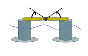
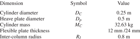
The aim of the test campaign was to produce response data for a simple flexible structure subject to first- and higher-order wave loads. The experiments were carried out in the deep water basin at DHI, Hørsholm, Denmark in 2020. The set-up consisted of the floating structure shown in figure 1(a), which was used as a generic representation of a semi-submersible wind turbine substructure, subjected to wave loads only. A sketch of the wave basin and model position is shown in figure 1(b), also marking the positions of the eight wave gauges. The position of the model was chosen to provide easy access via the main bridge in the basin. Although the asymmetric lateral placement may lead to asymmetric re-reflected waves from the sidewalls, we regard this effect to be minor due to the small extent of the structure relative to the basin dimensions. We will use the signal from a wave gauge at the centre of the floater position  $([x,y] = [5\ {\rm m},20\ {\rm m}])$ measured without the model in place as input to the numerical model. The floater response in six degrees of freedom was measured using a motion tracking system, where two infrared cameras measured the relative position of four to five reflective markers at the top of each cylinder and the centre position. Further, a six-degree-of-freedom accelerometer was positioned on top of each cylinder.
(a) Photo of the floating structure in the test basin, (b) schematic side view of floater with the flexible hinge plates drawn in black, (c) top-view diagram of experiment set-up with wave gauges (blue) and floating structure (green) in the wave basin.

The flexible floater was constructed from two rigid cylinders with thin heave plates. The structure was connected above water by a top beam made of two separate rigid beams, connected by a flexible aluminium plate acting as a hinge, which resulted in a flexible degree of freedom. The main dimensions of the structure are given in table 1. Two configurations of the flexible hinge were tested, henceforth denoted the single and double layout. The double layout had two flexible plates mounted between the rigid top beams, as shown schematically in figure 1(c) with the flexible plates marked in black. The bottom plate is marked as a dashed line as this was removed to achieve the single layout. The station keeping was achieved by four mooring lines, two fore and two aft, with pretension  $T_0 = 3$ N in each, and instrumented with force gauges attached to all four lines.
Main dimensions of floater. The / refers to the single/double flexible plate layout.
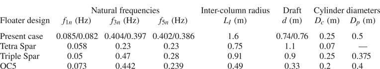
The rigid-body natural frequencies and inter-column distance of the floater were designed to match previously tested floater designs: TetraSpar (Madsen et al. Reference Madsen, Nielsen, Bredmose, Borg, Pegalajar-Jurado and Lomholt2017; Borg et al. Reference Borg, Jensen, Urquhart, Andersen, Thomsen and Stiesdal2020), TripleSpar (Bredmose et al. Reference Bredmose2017), OC5 (Robertson et al. Reference Robertson2017) and Cener (Boulluec Reference Boulluec2019), shown in model scale for a length scale ratio of  $\lambda _s = 1\,:\,60$ in table 2. The present floater concept is presented in the top row with both the single and double layout. We observe that the rigid-body natural frequencies decrease by 1 %–4 % from the single to double layout. This tendency is also observed in the numerical model, and is assumed to be caused by the larger mass and draft of the double layout floater.
Comparison of rigid-body natural frequencies  $f_n$ and main dimensions for different floating offshore wind floater concepts given in 1 : 60 model scale. Parameters $D_C$ and $D_p$ are the cylinder and heave plate diameter, respectively, and the / refers to the single/double layout.
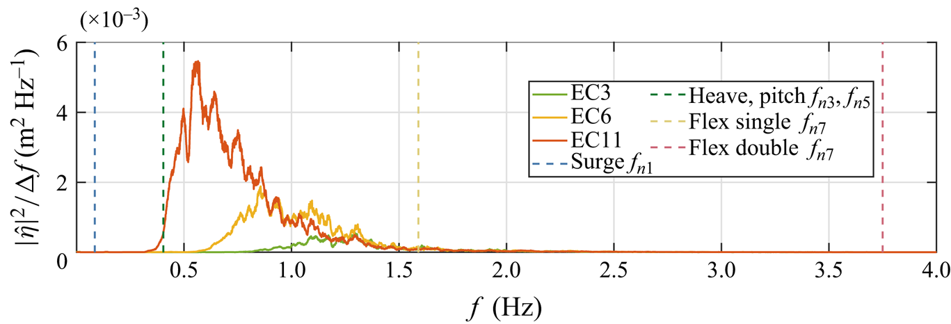
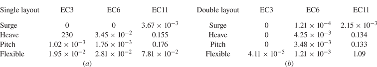
The floater was tested in three different sea states with different significant wave heights  $H_s$ and peak periods $T_p$, with a Pierson–Moskowitz spectral shape. The values are shown in table 3 and power spectral density (PSD) curves of free-surface elevation are shown in figure 2, where the natural frequencies of the rigid-body and flexible modes for the single and double layout are also shown. Irregular realisations of each sea state were run with a duration of 30 min (3 h full scale). The sea state definitions go back to earlier test campaigns for floating wind turbine response by the Technical University of Denmark (DTU) and DHI Denmark, e.g. Bredmose et al. (Reference Bredmose2017) and Orszaghova et al. (Reference Orszaghova, Taylor, Wolgamot, Madsen, Pegalajar-Jurado and Bredmose2021), where EC3 has been used for conditions below rated wind speeds ( ${<}11$ m s $^{-1}$ in full scale for the DTU 10 MW reference wind turbine) and EC6 has been used above the rated wind speed. We will denote these states as ‘mild’ and ‘intermediate’, although the significant wave height is quite large for both. EC11 represents an extreme sea state with a return period of several years, and represents a storm condition with wind speeds above the cut-out wind speed. The table also includes the Ursell number and wave steepness, based on the significant wave height and wavelength at the spectral peak. The steepness measure is 0.005 for both EC3 and EC6 and a bit smaller for EC11 due to breaking limitations. The Ursell number increases through the states and indicates that the nonlinearity is strongest for EC11.
Environmental conditions used in the experiments in terms of significant wave height  $H_s$, peak period $T_p$, sea state steepness ${H_s}/{L_p}$ and Ursell number $U = {H_s\lambda _p^2}/{h^3}$. Model scale values are given in parentheses.

Measured free-surface elevation PSD functions (solid curves) for each sea state and floater natural frequencies (dashed vertical lines).
3. Response analysis with harmonic separation and amplitude scaling
3.1. Harmonic analysis of floater response
To the knowledge of the authors, this work is the first to utilise the four-phase harmonic separation method of Fitzgerald et al. (Reference Fitzgerald, Taylor, Eatock Taylor, Grice and Zang2014) to analyse the response of a floating body. Four-phase separation was previously utilised to evaluate wave forcing for a bottom-fixed cylinder in Kristoffersen et al. (Reference Kristoffersen, Bredmose, Georgakis, Branger and Luneau2021), and resonant responses inside a narrow gap between two fixed boxes in Zhao et al. (Reference Zhao, Taylor, Wolgamot and Eatock Taylor2021). The separation method requires each distinct wave realisation to be run four times, each with a phase shift of 90 $^\circ$ in wave paddle motion from the previous. Harmonic separation is then carried out through the following combinations of phase-shifted signals, see Fitzgerald et al. (Reference Fitzgerald, Taylor, Eatock Taylor, Grice and Zang2014):
 $$\begin{gather} Q^{(1)} = \frac{Q_0-Q_{90}^H-Q_{180}+Q_{270}^H}{4} = Aq_{11}\cos\phi + A^2f_{D}\cos \phi + A^3q_{31}\cos \phi +O(A^5), \end{gather}$$
 $$\begin{gather}Q^{(2)} = \frac{Q_0-Q_{90}+Q_{180}-Q_{270}}{4} =A^2q_{22}\cos 2\phi+A^4q_{42}\cos 2\phi + O(A^6), \end{gather}$$
 $$\begin{gather}Q^{(3)} = \frac{Q_0+Q_{90}^H-Q_{180}-Q_{270}^H}{4} =A^2 f_{D}\cos 3\phi+ A^3q_{33}\cos3\phi + O(A^5), \end{gather}$$
 $$\begin{gather}Q^{(0+4)} = \frac{Q_0+Q_{90}+Q_{180}+Q_{270}}{4} = A^2q_{20} + A^4q_{40} + A^4q_{44}\cos 4\phi + O(A^6). \end{gather}$$
 Here,  $Q$ is the response, with the subscripts referring to the chosen phase shift of the signal and superscript in parenthesis defining the harmonic, while superscript $H$ is the Hilbert transform. Further, A is the amplitude, $\phi$ is the phase of the wave component and $q_{mn}$ is the wave-to-response transfer function with $m$ the power of the amplitude and $n$ the frequency harmonic. The equations are given for a monochromatic wave for simplicity, but the linear combinations are applicable to irregular wave time series. Note that the response from the Morison drag term, which is given separately above, will be visible in both the first- and third-harmonic response time series. However, due to the $u|u|$-term, where u is the local horizontal fluid velocity for drag, resulting in a squared amplitude dependence, amplitude analysis can be applied to separate and identify the driving forces behind the first- and third-harmonic responses, as done in Orszaghova et al. (Reference Orszaghova, Taylor, Wolgamot, Madsen, Pegalajar-Jurado and Bredmose2021).
To minimise the effect of harmonic leakage, the four-phase-shifted signals were carefully aligned. Alignment was carried out by pairwise alignment of first the 0 $^\circ$ and 180 $^\circ$ signals and the 90 $^\circ$ and 270 $^\circ$ signals, followed by fitting of the two pairs such that all four signals were aligned in time. Alignment of two signals was obtained by computing and plotting the odd- and even-harmonic spectra, with one signal time shifted relative to the other for a number of different time shifts within a realistic range. The appropriate time shift was the one that resulted in the highest spectral energy in the linear wave range and the lowest outside of it for the odd harmonic, and the opposite for the even harmonic. For alignment of all four signals, the same approach with pairwise shifting of the 0 $^\circ$ and 180 $^\circ$ signals relative to the 90 $^\circ$ and 270 $^\circ$ was applied. The shift which resulted in the least spectral energy in the linear frequency range for the higher harmonics was chosen. Details of the analysis of signal alignment are shown in Appendix A for the pitch response to EC3.
Figure 3 shows the PSD curve for free-surface elevation and phase separated floater pitch,  $\xi _5$ for all three sea states in figures 3(a), 3(b) and 3(c), respectively. Further, the modulus of the response amplitude operator (RAO) is shown in figure 3(d), determined experimentally for each sea state. The natural frequency, $f_n$, was found through free decay tests and is shown as a dashed black line. We observe that pitch motion for EC3 and EC6 is dominated by nonlinear resonance at the natural frequency, occurring at the zeroth and fourth harmonic. We anticipate that this is caused by second-order sub-harmonic forcing, as it is reasonable to assume that the term $A^4q_{40}$ is negligible, and the fourth-harmonic term $A^4q_{44}\cos 4\phi$ is a sum-frequency term which thus corresponds to super-harmonic response. For EC11, the natural frequency lies within the linear frequency range and the resonant pitch response is therefore dominated by the first harmonic, containing the linear and drag-induced response. The response peaks at $f= 0.082$ Hz, which are present for all three sea states, correspond to the surge natural frequency and clearly show the strong coupling between surge and pitch.
Power spectral density plots of four-phase separated response in pitch  $\xi _5$ for the single layout for EC3 (a), EC6 (b) and EC11 (c). The modulus of the RAO is shown for all sea states in (d).

For the flexible degree of freedom shown in figure 4 (using the same layout as figure 3), the natural frequency lies within the linear spectrum for EC3 (figure 4a) and EC6 (figure 4b), and we thus observe that flexible resonant response is driven by the first harmonic (linear and drag forcing). Also, for EC11, the maximum flexible response lies within the linear frequency range close to the free-surface elevation peak frequency. The flexible mode resonance is thus dominated by the first harmonic, but with significant contribution from the second harmonic, showing that second-order superharmonic forcing is a significant driver of the flexible response for EC11.
Power spectral density plots of four-phase separated response in the flexible mode  $\xi _7$ for the single layout for EC3 (a), EC6 (b) and EC11 (c). The modulus of the RAO is shown for all sea states in (d).

We next apply the harmonic decomposition to the double layout flexible response in figure 5. Here, the flexible mode natural frequency lies at approximately 3, 5 and 7 times the peak frequency for EC3, EC6 and EC11, respectively. The largest response occurs within the linear frequency range, with an amplitude significantly lower than for the single layout response. At the natural frequency, however, the resonant response is driven by increasing harmonic content for each sea state. The second-harmonic response dominates the resonance for EC3, (figure 5a), while the largest resonance in EC6 (figure 5b) occurs within the third harmonic, however, with a smaller margin. Although the resonance amplitude is very small for EC11, we see that it is dominated by the fourth-harmonic spectral amplitude, which is slightly larger than the other harmonics. The dominance of the resonant response by higher harmonics for increasing sea state is well aligned with the growth of Ursell number and decrease of peak frequency for each step to a larger sea state. We note that, despite the large difference between  $f_p$ for EC11 and $f_n$ for the double layout flexible mode, we observe some first-harmonic resonant response additional to the higher-harmonic response. We note that, in the four-phase harmonic separation analysis, the first-harmonic signal also contains energy from the fifth harmonic. This contribution may thus explain the large amplitude of this signal so far away from the spectral peak.
Power spectral density plots of four-phase separated response in the flexible mode  $\xi _7$ for the double layout for EC3 (a), EC6 (b) and EC11 (c). The modulus of the RAO is shown for all sea states in (d).

3.2. Amplitude analysis
In the previous section, we analysed the harmonic content of the floater response by separation into four harmonics. In the two even-harmonic signals, we were able to identify forcing terms based on the harmonic and the frequency content, but for the first- and third-harmonic signals, the analysis does not distinguish between the inviscid potential-flow forcing and viscous drag forcing, which both contribute to the first and third harmonics. We therefore proceed here with analysis of the amplitude scaling of the resonant responses to shed further light on the dominant forcing terms. We will analyse surge, pitch and flexible responses for all three sea states. The analysis is conducted on the odd- and even-harmonic signal content, instead of all four outputs of the harmonic separation analysis. This is because we will later utilise the results to explain possible discrepancies between the experiment and the numerical model, which reproduces only first- and second-order induced responses, and is thus not able to reproduce all terms in the third and fourth harmonics.
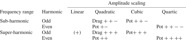
Table 4 presents the nonlinear forcing terms ordered by harmonic content, frequency range and amplitude dependence. We observe that all odd-harmonic forcing contributions scale with distinct powers of the first-order wave amplitude, allowing us to separate each contribution through an analysis of amplitude dependence. Note that, in the super-harmonic range, we might observe a response with a linear amplitude dependence due to the high tail of the Pierson–Moskowitz wave spectrum. Amplitude scaling analysis has previously been presented by Pierella et al. (Reference Pierella, Bredmose and Dixen2021) for analysis of nonlinear wave generation effects and by Orszaghova et al. (Reference Orszaghova, Taylor, Wolgamot, Madsen, Pegalajar-Jurado and Bredmose2021) for analysis of the pitch response of the TetraSpar floating wind turbine in severe wave conditions. The latter study concluded, for the even harmonic, that second-order potential forcing dominates, and for the odd harmonic that Morison drag – rather than third-order potential forcing – dominated the sub-harmonic pitch response in a severe sea state.
Data analysis understanding chart. Potential (Pot) flow forcing terms up to fourth order and drag forcing terms grouped by the frequency range, harmonic content and amplitude scale of respective forcing/response terms.
To extract the amplitude dependence of the resonant response from the present long irregular time series, we isolate the resonant response and wave time signals, identify the biggest peaks in each, and subsequently seek a correlation between the two series of peak amplitudes. For sub-harmonic resonant modes, the peak extraction process is illustrated in figure 6. Here, positive peaks are found in a given odd- or even-harmonic response signal, which has been bandpass filtered around the natural frequency. A suitable time interval in which these peaks occur is then defined – here the interval limits are chosen as the midpoint in time between peaks – and the corresponding peak of the first-harmonic free-surface elevation envelope  $|(\eta ^{(1)})^H|$ is extracted. For the super-harmonic resonant response, the method was reversed to a wave-by-wave analysis: for any given peak in the first-harmonic wave envelope, an interval around it is defined, and the maximum response peak in the interval is located. This approach was chosen to avoid multiple extreme response counts within a single large wave event. After extraction of response peaks and first-order wave envelope peaks, we sort both series of peaks individually in descending order and plot the largest 30 % of odd- and even-harmonic response peaks ( $\xi _{peaks}$) against the sorted first-harmonic wave envelope peaks ( $\eta _{peaks}$) in a log–log plot, and fit manually linear, quadratic and cubic correlation lines. The amplitude scaling is then extracted from the slope of the peak correlation curve.
Amplitude analysis method for surge. (a) Excerpt of  $\xi _1(t)$ band pass filtered around $f_{n1}$, peaks and halfway distance marked. (b) First-harmonic wave signal (blue) and corresponding wave envelope (yellow) with max values of the envelope in each interval (green).

Figure 7 shows a log–log plot of sorted response peaks  $\xi _{peaks}$ of the odd- and even-harmonic surge (a,c,e) and pitch (b,d,f) responses for EC3 (a,b), EC6 (c,d) and EC11 (e,f) as a function of the sorted corresponding maxima of the first-harmonic free-surface elevation envelope, $\eta _{peaks}$. The surge response has been manually fitted with second- and third-order correlation lines, and the pitch has been fitted with first- and second-order lines, where the former is included to illustrate proportionality to the linear wave peaks.
Log–log plot of resonant surge (a,c,e) and pitch (b,d,f) response peaks as a function of the first-harmonic wave envelope peaks for sea state EC3 (a,b), EC6 (c,d) and EC11 (e,f). The dashed lines are linear, quadratic and cubic order polynomial regressions.

In surge, the dominant resonant response is even harmonic and the peaks display a clear quadratic proportionality to the first-harmonic free-surface elevation for all three sea states. This shows, as expected, that second-order potential-flow forcing (see table 4) drives the surge resonance. The odd-harmonic peaks (dark blue), which are smaller than the even, are shown with both quadratic and cubic correlation lines, following the cubic closest for EC3 (a) and EC6 (c), and the quadratic for EC11 (e). This indicates that third-order potential-flow forcing dominates the odd-harmonic surge resonance for EC3 and EC6. The quadratic amplitude behaviour in EC11 can be due to either dominance by drag forcing or amplitude-dependent damping that may change the response scaling. Several studies have concluded that the damping can be sea state dependent, see for example Pegalajar Jurado & Bredmose (Reference Pegalajar Jurado and Bredmose2019). One well-known example is the local Morison drag term with relative velocity  $d f=\tfrac {1}{2}\rho C_D D (u-\dot {x})|u-\dot {x}|$, where $\rho$ is the fluid density, $u$ the local horizontal fluid velocity, $\dot {x}$ the local structural velocity, $D$ a representative diameter and $C_D$ the drag coefficient. For $|\dot {x}|\ll |u|$, the forcing can be written as $df=\rho C_D((\tfrac {1}{2}u|u| - |u|\dot {x})$ and thus contains a damping term proportional to the wave amplitude. Given that the cubic forcing effect is initially largest, it seems less likely that the second-order drag forcing should become dominant for larger wave amplitude. Thereby increased damping for large wave amplitude seems the most plausible explanation for the transition from cubic to quadratic amplitude scaling of the odd-harmonic response. Due to the very low natural frequency in surge, there are significantly fewer peaks in the response time series compared with the other degrees of freedom, and our conclusions are thus subject to some uncertainty.
In pitch, the even-harmonic peaks are dominant for EC3 (figure 7b) and EC6 (figure 7d), both following the quadratic proportionality to the first-harmonic wave peaks. Thus, also for pitch, the second-order potential forcing is the predominant driver of resonant response in the sub-harmonic range. The odd-harmonic peaks for these sea states scale quadratically with the linear wave envelope, indicating drag-dominated resonant response in pitch. In EC6, the largest peaks of the odd-harmonic response follows the linear proportionality line, indicating some linear forcing for the biggest wave peaks. Finally, for EC11 (figure 7f), the pitch natural frequency lies within the linear wave spectrum (see figure 2), and the resonant response is therefore predominantly linear, as seen by the large-amplitude odd-harmonic peaks following the first-order polynomial closely. It should be noted that the even-harmonic peaks show a smaller than quadratic proportionality to the first-harmonic wave envelope for EC11 and the largest peaks of EC6, even though there are no linear amplitude terms present in the even-harmonic response terms (see table 4 and (3.1)–(3.4)). This may also be explained by damping effects, that may subtract in the amplitude scaling power of the forcing term as outlined above for surge.
To analyse the super-harmonic system natural frequencies, amplitude analysis was carried out for the single layout flexible mode response, shown in figure 8. For the flexible mode resonance, the odd-harmonic peaks dominate for both EC3 (figure 8a) and EC6 (figure 8b), whereas odd and even are of similar magnitude for EC11, where  $f_{n7,s}$ lies at the upper end of the linear wave spectrum. The odd harmonic follows a linear scaling for the smaller peaks of EC3, transitioning towards quadratic slope for the larger wave crests ( ${>}0.045$ m) in EC3 and EC6. In EC11, the odd-harmonic scaling is again linear. Since, again, it is unlikely that a quadratic, dominant forcing effect can be overtaken by a linear effect, this behaviour can best be explained by linear dominance (small crests in EC3) followed by drag dominance (crests above 0.045 m) with amplitude-dependent damping effects becoming important in EC11 (crests larger than 0.1 m). For the even-harmonic response, a similar evolution is seen, with quadratic amplitude scaling in EC3 and linear amplitude scaling in EC6 and EC11. In further support for the importance of damping, we note that the response level as function of crest amplitude is not identical across the sea states. For fixed crest height, the even and odd responses become smaller for increasing sea state. This underlines the importance of the background sea state to the resonant response level and thus the importance of damping.
Log–log plot of sorted single layout flexible mode response peaks as a function of sorted first-harmonic free-surface envelope peaks fitted with linear and quadratic polynomial regressions.

The amplitude scaling analysis on the double layout flexible response has been omitted, as the results did not show clear scaling of the response, presumably due to the small resonant response amplitudes compared with the linear flexible mode response (see figure 5) and with the relatively large noise levels. Orszaghova et al. (Reference Orszaghova, Taylor, Wolgamot, Madsen, Pegalajar-Jurado and Bredmose2021) note that amplitude analysis is sensitive to noise in the signals, especially for smaller response levels. They performed the conditioning amplitude analysis for the resonant pitch response of a similar structure for the extreme sea state EC11 only, and argued that the mild and intermediate sea states showed too high levels of noise.
To compare the applicability of our simple amplitude analysis with the more in-depth and sophisticated form of analysis conducted in Orszaghova et al. (Reference Orszaghova, Taylor, Wolgamot, Madsen, Pegalajar-Jurado and Bredmose2021), the EC11 surge response conditioned on the linear wave envelope is shown as an example of the latter approach. The conditioning procedure entails only considering the largest  $N$ peaks in the wave signal and the $N$ corresponding response peaks. We then collect the peaks into groups containing peaks nos. 1–20, 2–21, 3–22 etc. and average over each group to limit the influence of noise. A second-order forcing proxy signal of the form $(\eta ^{(1)})^2$ is used instead of the linear wave envelope. By bandpass filtering the forcing proxy around the response natural frequency, the part of the forcing proxy signal that leads to second-order forcing of the specific resonant mode is isolated.
In Orszaghova et al. (Reference Orszaghova, Taylor, Wolgamot, Madsen, Pegalajar-Jurado and Bredmose2021) a forcing proxy of the form  $u^{(1)}|u^{(1)}|$ – with $u^{(1)}$ representing the linearised horizontal fluid velocity – is used to detect drag forcing. However, as this quantity scales with the wave amplitude squared, we will simply use $(\eta ^{(1)})^2$ as proxy for both the second-order potential-flow force and the drag force. Choosing the conditioned response peak – the biggest response peak adjacent to the conditioning second-order forcing proxy peak – retains the time pairing between the forcing and response terms, which may make the response conditioning approach more sensitive to noise in the response signals than the simple method presented here.
Figure 9 presents the EC11 surge response as a test case of response conditioning amplitude dependence analysis for comparison of the simple sorting method. Here, 21 averaged groups (corresponding to  $N=40$) of conditioned peaks are plotted against the conditioning second-order forcing proxy, allowing the quadratic amplitude scaling to be drawn as a linear regression forced through $(0,0)$. We observe a reasonably good linear correlation between the second-order forcing proxy and the conditioned even-harmonic response peaks. The odd harmonic is best fitted with a linear correlation with the second-order forcing proxy. Both these results confirm the observations made about the response amplitude scaling for EC11 surge based on the simple sorting method shown in figure 7: the even-harmonic response, which is driven by second-order potential-flow forcing, dominates the resonant surge response, and the smaller odd-harmonic response contribution is driven by drag forcing.
Response conditioned amplitude analysis for EC11, single layout surge response. Conditioned and averaged response peaks as a function of squared linear free-surface elevation envelope peaks.

The conditioning amplitude dependence analysis, where the time correlation of the forcing proxy and the response is retained, was found to be unsuccessful for a number of other modes and sea states. This was also observed in Orszaghova et al. (Reference Orszaghova, Taylor, Wolgamot, Madsen, Pegalajar-Jurado and Bredmose2021), where the amplitude method is described as sensitive to clustering and noise in the data. We suggest that these errors might be due to a memory effect in the resonant response, which causes slow decay of large-amplitude resonance and as such decouples large free-surface elevation peaks from large response peaks.
4. Response model with second-order loads
The numerical model for the floater was designed to test how much of the floater response we could reproduce with linear loads, second-order inviscid loads and drag loads. Another significant incentive is to test the eigen-value decomposition force model (Bredmose & Pegalajar-Jurado Reference Bredmose and Pegalajar-Jurado2021) in conjunction with a frequency-domain response model, as this combination can be of great practical value in early design stages. The force model is based on eigen-value decomposition of the quadratic force transfer functions. The decomposition reduces the computational effort of a second-order force time series, from a double sum over the number of discrete frequencies to a sum over the number of active eigen-values of pseudo-time series, computed using Fast Fourier Transform (FFT) with the eigen-vector as the transfer function. The precision of the model is equivalent to that of Sharma & Dean (Reference Sharma and Dean1981), but the computational effort is comparable to that of a linear Morison force model. In the present work, the second-order force model is extended to include forcing in the heave degree of freedom.
4.1. Mechanical model
We compute the hydrodynamic coefficients for each cylinder separately and neglect effects from hydrodynamic interactions between the two cylinders. With an inter-column distance  $>6D_C$ we assume any radiation to be negligible.
The hydrodynamic loads are applied in the cylinder reference frame (subscript  $C$ for cylinder, $L$ and $R$ for left and right) as shown for the left cylinder in figure 10(a). The force transfer matrix $\boldsymbol{\mathsf{T}}_F$ is then used to transform local loads to the global reference frame (subscript $G$), shown in figure 10(b). The value of $\boldsymbol{\mathsf{T}}_F$ is found though simple force balances
 \begin{equation} \boldsymbol{\mathsf{F}}_G=\begin{bmatrix}F_{1,G} \\ F_{3,G} \\ F_{5,G} \\ F_{7,G} \end{bmatrix} = \begin{bmatrix} 1 & 0 & 0 & 1 & 0 & 0 \\ 0 & 1 & 0 & 0 & 1 & 0 \\ 0 & R_I & 1 & 0 & -R_I & 1 \\ -\dfrac{a}{2} & \dfrac{R_I}{2} & \dfrac{1}{2} & \dfrac{a}{2} & \dfrac{R_I}{2} & - \dfrac{1}{2} \end{bmatrix}\boldsymbol{\cdot} \begin{bmatrix} F_{1,L}\\ F_{3,L} \\ F_{5,L}\\ F_{1,R}\\ F_{3,R} \\ F_{5,R} \end{bmatrix} = \boldsymbol{\mathsf{T}}_F\boldsymbol{\cdot}\begin{bmatrix} \boldsymbol{F}_L\\\boldsymbol{F}_R \end{bmatrix}. \end{equation}
(a) Forces applied on the left cylinder (red) and local response reference frame (black). (b) Schematic of the floater with local and global reference frames.

Likewise, the response transfer matrix is used to transform the global response into local coordinates as follows:
 \begin{equation} \begin{bmatrix} \xi_{1,L} \\ \xi_{3,L} \\ \xi_{5,L} \\ \xi_{1,R} \\ \xi_{3,R} \\ \xi_{5,R}\end{bmatrix} = \begin{bmatrix} 1 & 0 & 0 & 0 \\ 0 & 1 & R_I & \frac{1}{2}R_I\\ 0 & 0 & 1 & \frac{1}{2} \\ 1 & 0 & 0 & 0\\ 0 & 1 & -R_I & \frac{1}{2} R_I\\ 0 & 0 & 1 & -\frac{1}{2} \end{bmatrix} \boldsymbol{\cdot} \begin{bmatrix} \xi_{1,G}\\ \xi_{3,G} \\ \xi_{5,G} \\ \xi_{7,G} \end{bmatrix} = \boldsymbol{\mathsf{T}}_\xi \boldsymbol{\xi}_G . \end{equation}
 The equations of motion are solved in the global frame of reference using constant system matrices of mass  $\boldsymbol{\mathsf{M}}$, added mass $\boldsymbol{\mathsf{A}}$, damping $\boldsymbol{\mathsf{B}}$ and stiffness $\boldsymbol{\mathsf{C}}$, which are determined for each identical cylinder separately and transformed to the global reference frame using $\boldsymbol{\mathsf{T}}_F$
 \begin{equation} (\boldsymbol{\mathsf{M}}+\boldsymbol{\mathsf{A}})_G\ddot{\boldsymbol{\xi}}_G+\boldsymbol{\mathsf{B}}_G\dot{\boldsymbol{\xi}}_G +(\boldsymbol{\mathsf{C}}_G+\boldsymbol{\mathsf{C}}_{f,m})\boldsymbol{\xi}_G=\boldsymbol{\mathsf{F}}_G. \end{equation}
In this equation  $\boldsymbol{\mathsf{A}}$ is the added $\boldsymbol{\mathsf{C}}_{f,m}$ is the linearised stiffness matrix for the mooring system, defined in the global reference frame as
 \begin{equation} \boldsymbol{\mathsf{C}}_{f,m} = \begin{bmatrix} k_1 & 0 & a k_1 & 0\\ 0 & 0 & 0 & 0 \\ ak_1 & 0 & 2R_IT_0 +a^2 k_1 & 0\\ 0 & 0 & 0 & k_{7}+R_I T_0\end{bmatrix}. \end{equation}
Here,  $a = 0.14$ m is the free board, $T_0 = 3$ N is the mooring pre-tension and $k_1 = 41.22$ N m $^{-1}$ is the equivalent spring stiffness in surge. The parameter $k_{7}$ is a numerically fitted spring stiffness for the flexible plates, chosen such that the flexible natural frequency in the numerical model, $f_{n7}$, matches the experimental value determined from decay tests for each of the two layout configurations. The mass and added mass matrices are populated on the diagonal and the anti-diagonal
 \begin{equation} \boldsymbol{\mathsf{M}}_C =\begin{bmatrix} m_C & 0 & z_g m_C \\ 0 & m_C & 0\\m_C z_g & 0 & I_y \end{bmatrix} \quad \boldsymbol{\mathsf{A}}_C =\begin{bmatrix} a_{11} & 0 & a_{15} \\ 0 & a_{33} & 0\\a_{51} & 0 & a_{55} \end{bmatrix}. \end{equation}
Here, the heave added mass  $a_{33}$ is the added mass of a cylinder with a disk attached, neglecting interference between the cylinder and heave plate as it assumes that the entrained fluid is stationary relative to the cylinder (Moreno et al. Reference Moreno, Thiagarajan, Cameron and Urbina2016). The value of $a_{33}$ is found as a function of $D_c$, $D_d$, the water density, $\rho$, and the shape parameter $r_d={1}/{{\rm \pi} }\sqrt {D_d^2-D_c^2}$ as follows:
 \begin{equation} a_{33}= \tfrac{1}{12}\rho(2 D_d^3+{\rm \pi} D_d^2r_d-{\rm \pi}^3r_d^3 -{\rm \pi} 3D_c^2r_d). \end{equation}
 The surge and pitch added mass are found as the added mass of a finite length cylinder with bottom coordinate  $z_{bot}=-d$
 $$\begin{gather} a_{11} =-\rho \frac{{\rm \pi} D_C^2}{4}C_m z_{bot}, \end{gather}$$
 $$\begin{gather}a_{15} =a_{51} =- \frac{1}{2}\rho \frac{{\rm \pi} D_C^2}{4}C_m z_{bot} ^2 , \end{gather}$$
 $$\begin{gather}a_{55} =-\frac{1}{3}\rho \frac{{\rm \pi} D_C^2}{4}C_m z_{bot}^3, \end{gather}$$
where  $C_m=1$ is the added mass coefficient for surge and pitch.
The single-cylinder stiffness matrix has non-zero elements in the heave and pitch diagonal only
 \begin{equation} \boldsymbol{\mathsf{C}}_C = \begin{bmatrix} 0 & 0 & 0\\ 0 & \rho g A_C & 0 \\ 0 & 0 & \rho g I_{11}^A +m_C g (z_b-z_g) \end{bmatrix}, \end{equation}
where  $A_C = {{\rm \pi} D_C^2}/{4}$ is the cylinder water-plane area and $I_{11}= ({{\rm \pi} }/{4})({D_C}/{2})^4$ is the second moment of the area for the cylinder. The damping matrix $\boldsymbol{\mathsf{B}}$ is populated in the modal space using modal damping ratios found through decay tests. These are subsequently calibrated by matching the standard deviation of the numerical response time series to the corresponding measured response for each sea state and each degree of freedom. For the calibration, the time series are bandpass filtered with $f_{min}=0.06$ Hz and $f_{max}=2$ Hz for the single layout and $f_{max}=4$ Hz for the double layout to reduce the impact of noise. The damping ratios used for each sea state and configuration are shown in table 5(a) and (b), respectively. Note that, for the configurations where the damping ratio is 0 as well as for the heave, EC3, single layout, we were unable to match the standard deviation for the measured response with the numerical model. For the double layout flexible degree of freedom, the damping ratio for EC6 has been adjusted to match the measured spectral peak, and the signal standard deviation for the model exceeds the experimental by 12 % due to an over-prediction of the linear response.
Modal damping ratios of the single and the double layout calibrated for the three sea states.
4.2. Force model
For the force expressions, the following convention will be used: the order of the force is given by the superscript in parenthesis, the degree of freedom by the first number of the subscript and a second number in the subscript will refer to a specific component of the force. For example,  $F^{(2)}_{31}$ refers to the second-order heave Froude–Krylov force containing the time derivative of the second-order potential. The corresponding second-order QTF is denoted $\mathcal {F}_{31}$.
The formulation of the solution to the second-order wave problem is directly adapted from Bredmose & Pegalajar-Jurado (Reference Bredmose and Pegalajar-Jurado2021), using double-sided frequency vectors and complex notation to include both sub- and super-harmonics in the same QTFs. All force terms are derived through manipulation of the first- and second-order velocity potential formulations, which are shown below in non-dimensional form, scaled with  $\tilde {\phi }= \phi h^{-3/2}g^{-1/2}$, $\hat {\tilde {B}}=\hat {B}h^{-3/2}g^{-1/2}$, non-dimensional angular frequency $\varOmega = \omega \sqrt {h/g}$ and non-dimensional wavenumber $\kappa = kh$.
 $$\begin{gather} \tilde{\phi}^{(1)} = \sum_{j=-N}^N \hat{\tilde{B}}_j\, {\rm e}^{{\rm i}(\omega_jt-k_jx)}\frac{\cosh k_j(z+h)}{\cosh k_jh}, \end{gather}$$
 $$\begin{gather}\tilde{\phi}^{(2)} = {\rm i} \sum_{m=-N}^N \sum_{n=-N}^N\mathcal{T}_\phi \hat{\tilde{B}}_m\hat{\tilde{B}}_n\, {\rm e}^{{\rm i}((\omega_m+\omega_n)t-(k_n+k_m)x)}\frac{\cosh( k_m+k_n)(z+h)}{\cosh (k_m+k_n)h}. \end{gather}$$
Here,  $N$ is the number of positive frequencies, while $\hat {B}_j$ and $k_j$ are the complex velocity potential Fourier amplitudes and the wavenumber corresponding to angular frequency $\omega _j$, respectively. The variables are made double-sided by $\hat {B}_{-j} = \hat {B}_j^*$ and $k_{-j} =-k_j$, where $^*$ refers to the complex conjugate. Also, $\hat {B}$ relates to the complex free-surface elevation Fourier amplitude $\hat {A}$ through $\hat {B}_j = ({ig}/{\omega _j})\hat {A}_j$ and $\mathcal {T}_\phi$ is the second-order velocity potential QTF.
In surge and pitch, both first- and second-order hydrodynamic loads are taken from Bredmose & Pegalajar-Jurado (Reference Bredmose and Pegalajar-Jurado2021), using the QTFs derived for slender surface-piercing cylinders of arbitrary depth. The second-order inertia force in surge includes Froude–Krylov and added mass terms to second order, a free-surface force (a leading-order integration of the free surface) as well as an axial divergence force term, adapted from Rainey (Reference Rainey1995). The drag loads are approximated by a quasi-steady simplified Morison drag term, shown here for surge
 \begin{equation} F_D = \frac{1}{2}\rho D_C C_D \int_{-d}^0 u_1^2 \, {\rm d} z \varPsi(\bar{u}_1), \end{equation}
where  $\varPsi (\bar {u}_1)= \tanh (3\bar {u}_1/\sigma _{\bar {u}_1})$ is a smoothed approximation to sign( $\bar {u}_1$) and where $\bar {u}_1$ is the depth-averaged linear horizontal particle velocity and $\sigma _{\bar {u}_1}$ is the corresponding standard deviation. No motion-induced second-order terms are included. The effects of the heave plates on the horizontal loads are assumed negligible. A MacCamy–Fuchs correction is applied to the surge and pitch inertia coefficient in both first and second orders, as the limit of the slender-body range, $D_c/L<0.2$ where $L$ is the wavelength, is violated for $f> 1.1$ Hz i.e. below the flexible natural frequencies of both the single and double layout configurations.
The heave load consists of a Froude–Krylov force term, an added mass term and a drag term. The first-order components are
 \begin{align} F^{(1)}_{3} &=F_{3FK}+F_{3AM} \end{align}
 \begin{align} &=-\frac{{\rm \pi} D_C^2}{4} \rho g h\sum_{j=-N}^N \hat{\tilde{B}}_j{\rm i} \varOmega_j \frac{\cosh k_j(-d+h)}{\cosh \kappa_j} \, {\rm e}^{{\rm i}(\omega_jt-k_jx)} \end{align}
 \begin{align} &\quad +C_{m,hp}\frac{{\rm \pi} D_p^3}{6} \rho g \sum_{j=-N}^N \hat{\tilde{B}}_j \varOmega_j \kappa_j \frac{\sinh k_j(-d+h)}{\cosh \kappa_j} \,{\rm e}^{{\rm i}(\omega_jt-k_jx)}, \end{align}
where the heave plate added mass coefficient is given by  $C_{m,hp} = {a_{33}}/{\frac {4}{3}{\rm \pi} \rho ({D_P}/{2})^3}$. At second order there are five distinct force components: $\mathcal {F}_{31}$ relating to the Froude–Krylov force from the second-order potential, $\mathcal {F}_{32}$ containing the axial divergence term, $\mathcal {F}_{33}$ for second-order Eulerian acceleration added mass force and $\mathcal {F}_{34}$ is the Lagrangian acceleration added mass term. The quadratic transfer functions for all components of the second-order heave inertia forces are
 $$\begin{gather} \mathcal{F}_{31}= \mathcal{T}_\phi (\varOmega_m+\varOmega_n) \frac{\cosh ((k_m+k_n)(-d+h))}{\cosh(\kappa_m+\kappa_n)}, \end{gather}$$
 $$\begin{gather}\mathcal{F}_{32} = \frac{1}{2}\kappa_m\kappa_n \frac{\cosh((k_m-k_n)(-d+h))}{\cosh \kappa_m \cosh \kappa_n}, \end{gather}$$
 $$\begin{gather}\mathcal{F}_{33} =-\mathcal{T}_\phi (\varOmega_m+\varOmega_n) (\kappa_m+\kappa_n) \frac{\sinh((k_m+k_n)(-d+h))}{\cosh{(\kappa_m+\kappa_n)}}, \end{gather}$$
 $$\begin{gather}\mathcal{F}_{34} = \frac{1}{2}(\kappa_m-\kappa_n)\kappa_m\kappa_n \frac{\sinh ((k_m-k_n)(-d+h))}{\cosh \kappa_m \cosh \kappa_n}. \end{gather}$$
The total heave force is then
 \begin{align} F^{(2)}_{3I} &= F^{(2)}_{3FK} +F^{(2)}_{3a} \end{align}
 \begin{align} &= \rho gh\frac{{\rm \pi} D_C^2}{4}{\rm i}\sum_{m=-N}^N\sum_{n=-N }^N \hat{\tilde{B}}_m\hat{\tilde{B}}_n( \mathcal{F}_{31}+\mathcal{F}_{32}) \,{\rm e}^{({\rm i}(\omega_m+\omega_n)t-(k_m+k_n)x)} \end{align}
 \begin{align} &\quad + \rho g\frac{{\rm \pi} D_p^3}{6}{\rm i} \sum_{m=-N}^N\sum_{n=-N }^N C_{m,hp}\hat{\tilde{B}}_m\hat{\tilde{B}}_n (\mathcal{F}_{33}+\mathcal{F}_{34})\, {\rm e}^{({\rm i}(\omega_m+\omega_n)t-(k_m+k_n)x)}. \end{align}
The drag force can be evaluated without the use of a QTF, as it is found by multiplying the first-order wave particle velocity on the heave plate with the modulus of itself
 \begin{equation} F^{(2)}_{3D} = \frac{1}{2}\rho {\rm \pi}\left(\frac{D_p}{2}\right)^2 C_{D,hp}\left.\left(\left.\frac{\partial\phi}{\partial z}^{(1)}\right|\left.\frac{\partial \phi}{\partial z}^{(1)}\right|\right)\right|_{z=z_{bot}}. \end{equation}
Here, the relative velocity is left out of the Morison drag formulation to allow the direct solution of the equation of motion in the frequency domain.
The drag coefficients  $C_D$ and $C_{D,hp}$ (table 6) for surge and pitch is determined for each sea state from Sumer & Fredsøe (Reference Sumer and Fredsøe2006), as the flow past the cylinders for EC3, EC6 and EC11 lie in the attached, separation and trans-critical flow regimes, respectively. The sea state-dependent drag coefficients for the heave plate are determined using an empirical formula presented in Li et al. (Reference Li, Liu, Zhao and Teng2013), which is a function of the depth-independent formulation of the Keulegan–Carpenter number $KC = {{\rm \pi} H_s}/{D_p}$ and the thickness-to-diameter ratio for the heave plate.
Sea state dependent Keulegan–Carpenter number  $KC$, Reynolds number $Re$ and drag coefficients $C_D$ for surge and pitch and $C_{D,hp}$ for heave.

5. Reproduction of the measured response
This section contains the validation of the numerical model against the experiment. The measured first-harmonic free-surface elevation at the floater position (without the floater in place) was used as model input. The numerical model was run using 70 active modes (number of eigenvalues) in the eigenvalue decomposition of the QTFs, as this was found to be the point of convergence for the standard deviation of the numerical response time series. While the number of active eigen-modes is significantly larger than recommended in Bredmose & Pegalajar-Jurado (Reference Bredmose and Pegalajar-Jurado2021), where 8 modes is suggested for a bottom-fixed monopile, the computational effort is still much smaller than  $O(N^2)$. The heave load QTF, which often includes large gradients, is believed to be the cause of the larger number of eigenvalues needed. For computing $\eta ^{(2)}$, Bredmose & Pegalajar-Jurado (Reference Bredmose and Pegalajar-Jurado2021) suggest solving the eigen-value problem for the QTF of the time derivative $\mathcal {T}_{\eta _t}$, and subsequently integrating the resulting time series. As $\mathcal {T}_{\eta _t} = (\varOmega _m + \varOmega _n) \mathcal {T}_{\eta }$ is a smoother function, the solution converges faster. In future work with the eigen-value decomposition method, this approach may be applied to potentially reduce the number of modes for the heave forcing.
The damping calibration was carried out for the full signal 0 $^\circ$ response, by matching the numerical model standard deviation (area under the PSD curve) to the experimental for all degrees of freedom simultaneously. The strongest effect from the calibration of modal damping occur at the spectral density around the corresponding natural frequency peak. Thus a mismatch in response far from the natural frequency will be compensated by spectral energy at the resonant response. This approach thus does not prevent errors in the harmonic components in the case of imprecise prediction of individual terms in the forcing model.
The model response is validated against experimental data, separated into the odd  $(Q_{odd} =({Q_{0}-Q_{180}})/{2})$ and even $(Q_{even} =({Q_{0}+Q_{180}})/{2})$ harmonic using two-phase harmonic separation. The odd harmonic contains all right-hand side terms in (3.1) and (3.3), and the even harmonic contains the right-hand side terms in (3.2) and (3.4). The numerical model response is also separated into harmonics, where the odd-harmonic response is due to linear and drag forcing, $\xi _{odd} = \xi ^{(1)}+\xi ^{(2)}_D$, while the even-harmonic model response is due to second-order potential forcing, $\xi _{even} = \xi ^{(2)}$. Two-phase separation is chosen over four-phase separation for simplicity, and because of the lack of third- and fourth-order loadings from the model. As the numerical model is unable to reproduce fourth-order forcing, the even-harmonic response consists of second-order sub-harmonic and super-harmonic contributions, which are easily distinguishable due to distinct frequency content.
The key degrees of freedom to validate are the pitch and flexible motion responses. Pitch because, for a floating wind turbine, this mode is crucial to control the turbine stability and power generation. The flexible degree of freedom is novel to experiments on floating wind substructures, and successful reproduction of the flexible response provides new possibilities in the early stages of floater design. Validation results are shown for EC6 and EC11 for the pitch and single layout flexible mode, and for EC6 for the double layout flexible mode. Validation of the model performance in surge and heave are included for EC6, single layout in § 5.3 and Appendix B, respectively, for completeness.
5.1. Pitch response
Starting with sub-harmonic resonant response, figure 11 shows the pitch response to sea state EC6, both numerical and experimental, including full signal, odd and even harmonics of the response, respectively. The measured response is shown in black, and the numerical model response curves are coloured yellow for the free-surface elevation (a,e,i), blue for the full signal 0 $^\circ$ phase response (b,f,j), green for the odd-harmonic response (c,g,k) and pink for the even-harmonic response (d,h,l). The first column (a–d) presents an excerpt of the time series, the centre column (e–h) shows PSD spectral plots and the right column shows exceedance probability plots. The model free-surface elevation, the yellow curves in (a,e,i), is the measured first-harmonic free-surface elevation, band-pass filtered to the linear frequency range, measured at the position of the centre of the floater without the floater in the basin. The experiment free-surface elevation is the 0 $^\circ$ signal measured in the same position.
By columns: time signal (a–d), PSD (e–h) and exceedance probability plots (i–l). By row: free-surface elevation (a,e,i), full signal (b,f,j), odd- (c,g,k) and even-harmonic responses (d,h,l) in pitch, EC6, single layout.

Starting with the exceedance probability plot for the total pitch signal, the numerical model shows a very good match for all probability levels except for the last two events. Also, the PSD for the full signal is matched reasonably, with a good match in the linear wave range and some underprediction below the natural pitch frequency. In the linear wave frequency range, the model accurately captures cancellation frequencies ( ${\sim }1.2$ Hz). Further insight is provided by the PSDs in rows 3 and 4 for the odd and even harmonics. The sub-harmonic response is dominated by the even-harmonic content, through the zeroth-harmonic second-order term $A^2q_{20}$ and is only partly reproduced by the numerical model. The second-order response statistics are matched very well by the model although, spectrally, the energy is seen to be concentrated relatively more around the natural frequency peaks. For the odd-harmonic response, the PSD matches the measurements well. The analysis in § 3.2 indicated that the subharmonic content was driven by drag. This is reproduced by the numerical model. Although the total and even response statistics are matched well, the odd peak statistics are seen to be over-predicted, probably as a consequence of the damping calibration strategy.
Following the same plot structure as figure 11, the model validation of the pitch response to the extreme sea state, EC11, is shown in figure 12. Here, the pitch natural frequency is located inside the linear wave spectrum, which causes a shift of the response to the odd-harmonic content, as was also seen in § 3.2, figure 7(d). For the full signal in row 2, the model matches the measured response statistics very well down to the last, say, 10 events. Also the full signal PSD is reproduced with good accuracy. Similar observations can be made for the odd-harmonic content, where though some over-prediction from the model is seen for  $P_{exc}<10^{-2}$.
By columns: time signal (a–d), PSD (e–h) and exceedance probability plots (i–l). By row: free-surface elevation (a,e,i), full signal (b,f,j), odd- (c,g,k) and even-harmonic responses (d,h,l) in pitch, EC11, single layout.

In § 3.2 we established that the dominating odd-harmonic resonant pitch response to EC11 grows with linear proportionality to the first-harmonic wave peaks. The numerical results for the odd harmonics can thus be expected to be dominantly driven by the linear forcing terms. On this background it is not surprising that the model response matches the measured well. Turning to the even-harmonic response, the model results show a substantial under-prediction. This is a consequence of the damping calibration, where the peak resonance frequencies are damped relative to the dominant odd-harmonic response, as seen in figure 12. Thus, even if the balance between the odd- and even-harmonic forcing contents is not correct in the model, the damping calibration can lead to a good reproduction of the total signal response statistics and PSD.
5.2. Flexible mode response
We now turn to the single layout flexible degree of freedom response. Figure 13 shows the comparison with the numerical model results for EC6, formatted in the same way as figure 11. For the single layout, the natural frequency of the flexible mode is located inside the linear wave spectrum. Similar to the pitch motion of EC11, the flexible degree of freedom response is thus dominated by the odd-harmonic response, predominantly linear, as seen in figure 8(b).
By columns: time signal (a–d), PSD (e–h) and exceedance probability plots (i–l). By row: free-surface elevation (a,e,i), full signal (b,f,j), odd- (c,g,k) and even-harmonic responses (d,h,l), respectively, the flexible mode, EC6, single layout.

The full response is well matched in both the PSD and peak statistics down to the very largest events. Also the time series show a good fit in the full signal. Similar observations are valid for the odd-harmonic content, which makes out the dominant part of the total response. A good match of the cancellation frequencies is seen in the response PSDs for both the total and odd-harmonic contents, indicating a good match of the modal matrices. For the even-harmonic response, some deviations to the measurements are seen, owing to a spectral dominance of the energy around the natural frequency, which in the damping calibration leads to some over-prediction for the response peaks above the 80 % quantile, i.e.  $P_{exc}<0.2$.
Further, for the extreme sea state EC11, figure 14 shows a comparison of the numerical model with the experimental results for the single layout flexible mode response. Again, the response is dominated by the odd harmonic, with the largest response PSD occurring around the wave peak frequency. We observe a good reproduction of the response statistics by the model, with a close match for all peaks in both the full signal and odd harmonic. Also, the full signal and the odd-harmonic model response time series match the measured signal well.
By columns: time signal (a–d), PSD (e–h) and exceedance probability plots (i–l). By row: free-surface elevation (a,e,i), full signal (b,f,j), odd- (c,g,k) and even-harmonic responses (d,h,l) in the flexible mode, EC11, single layout.

The PSD plots (f–h) all show a good match in the linear frequency range, with the odd-harmonic model response at  $f_{n7}$ damped. The even-harmonic model response again deviates from the measured for peaks larger than the 70 % quantile, i.e. $P_{exc}<0.3$. The even-harmonic model response PSD matches the experimental curve for frequencies smaller than the flexible mode natural frequency.
We now turn to the double layout. The natural frequency for this configuration is placed far from the peak frequency of the linear wave spectrum for all three sea states. The response is generally small, and the noise levels ( $10^{-4}$ degree for the angular response) from the measuring equipment are large in comparison. In figure 5 we saw that the resonant response was driven by the second, third and fourth harmonics, respectively, for increasing sea state severity with a small component forced by first-harmonic effects for all sea states. As we do not expect a linear flexible mode resonance in real designs, the performance of the model at the natural frequency is an interesting aspect, which may be valuable to identify the range of applicability of second-order numerical models. We here show one example of comparison of the model with the measured response, which is indicative of the model performance for all three sea states.
For the intermediate sea state EC6, figure 15 shows the model validation for the double layout flexible mode response, following the same structure as shown in previous figures. The full signal response statistics are matched with small deviations down to the largest three peaks. For the odd harmonic, the response statistics are overpredicted slightly. The full signal PSD shows generally low response levels compared with the level of noise in the full signal PSD, and slight model overprediction of the response in the linear wave range.
By columns: time signal (a–d), PSD (e–h) and exceedance probability plots (i–l). By row: free-surface elevation (a,e,i), full signal (b,f,j), odd- (c,g,k) and even-harmonic responses (d,h,l) in the flexible mode, EC6, double layout.

As the response level at the natural frequency is adjusted to match the full signal standard deviation through the damping calibration, the resonant response is well matched. A slight underprediction is seen in the odd harmonic and the even harmonic shows a small overprediction. The even-harmonic response statistics are poorly matched by the model, as the response mostly consists of noise and some resonance.
In § 3.1, we showed for the double layout flexible response to EC6 that the third-harmonic forcing is dominant at  $f_{n7} = 3.74$ Hz. This can mean both drag (which is second order in amplitude) and third-order potential forcing, which the model is unable to reproduce. We observe that both the odd- and even-harmonic model responses contain the resonant response.
5.3. Surge response
Besides the analysis for floater pitch and flexible motion, we also show an example of the model's performance in surge and heave (shown in Appendix B). Figure 16 shows the comparison of the numerical model with the measured surge response for the intermediate sea state EC6. In line with figure 7, we see that the surge response is dominated by subharmonic resonance. Note that this degree of freedom is an example of zero damping, where the calibration of the model response standard deviation did not succeed, presumably due to inaccuracy in the second-order force.
By columns: time signal (a–d), PSD (e–h) and exceedance probability plots (i–l). By row: free-surface elevation (a,e,i), full signal (b,f,j), odd- (c,g,k) and even-harmonic responses (d,h,l) in surge, EC6 single layout.

The full signal response statistics are matched by the model only for  $P_{exc}>0.3$, and underpredicted for the 30 % largest response crests. Large overpredictions in the odd-harmonic and underpredictions in the even-harmonic response statistics are seen. These are viewed as a consequence of the model being unable to reproduce the measured response level (see table 5) even with zero damping.
The even-harmonic PSD plot (16h) shows significant underprediction of the surge resonance, whereas the small response levels at the pitch natural frequency ( $\,f_{n5}=0.38$ Hz) are well matched. The odd-harmonic PSD is well matched by the model, aside from the large resonant peak at $f_{n1}$, an effect of the absence of damping in surge, which results in the general response level being overpredicted.
In the amplitude analysis (§ 3.2, figure 7) we observed cubic proportionality between the first-harmonic free-surface peaks and the odd-harmonic surge response peaks, suggesting that the odd-harmonic surge response is mostly due to third-order potential-flow forcing. However, as the model is unable to reproduce cubic effects, the response due to drag must be overpredicted.
6. Discussion and conclusions
A series of experiments have been carried out in a deep water wave basin, testing the response of a flexible semi-submersible floating structure with heave plates. The experimental results have been analysed with regards to harmonic content and amplitude scaling, and the response of three rigid-body degrees of freedom and the flexible bending mode has been remodelled by means of a linear response model including second-order Morison and Rainey (Reference Rainey1995) force terms.
The experimental results were analysed with four-phase harmonic separation, which allowed us to extract time series of the zeroth- and fourth- and first- to third-harmonic contents. With the purpose of identifying the forcing mechanisms behind the response, further analysis for the amplitude scaling was conducted, to distinguish between drag and inertia contributions in the odd harmonic content. The analysis can be summarised as follows:
• The sub-harmonic response is generally driven by second-order potential-flow forcing.
• The surge resonance is dominated by even harmonic second-order difference frequency forcing. The odd-harmonic response is 10 times smaller and driven by drag and third-order potential-flow forcing, depending on the sea state.
• Pitch resonance is driven by even harmonic second-order sub-harmonic forcing for the mild and intermediate sea state, with the odd harmonic driven mostly by drag. For the strongest sea state, the pitch resonant mode is excited by linear potential forcing, as the natural frequency lies within the linear spectrum.
• For the single layout flexible mode, the response peaks are driven mostly by linear forcing and drag for all three sea states, with the second-order sum-frequency even-harmonic response having increasing relative importance for increasing severity of the sea state.
• For the double layout, the flexible mode was driven by second-, third- and fourth-harmonic contents for increasing severity of the sea states.
• The simple amplitude analysis method was compared with the more elaborate response conditioning approach for the case of surge motion in the extreme sea state with consistent results.
• For some of the responses, the power of the amplitude scaling was seen to decrease for large response levels. For example, the odd-harmonic response scaled first linearly with wave amplitude, then quadratically and then again linearly. Wave amplitude proportional damping has been suggested to cause this effect.
The numerical model incorporated first- and second-order forcings, evaluated at the equilibrium position of the structure. A modal damping calibration was made for each sea state, to ensure that the standard deviation of response matched the measured values. After this calibration, the model was generally able to reproduce the response statistics with good accuracy for pitch, heave and the flexible mode. This was also the case for the resonant modes, which were dominated by the odd-harmonic response. For surge, however, the total response was under-predicted, even with a zero damping level.
Further insight into the model performance was obtained by separate analysis on the odd- and even-harmonic contents of the response. Hereby, the accuracy and balance between their contributions was assessed. Generally, the odd-harmonic response was reproduced with reasonable accuracy, with some over-prediction for the cases that did not match. For the even-harmonic content, the response was generally under-predicted for the low-frequency rigid-body modes and over-predicted for the flexible modes. This demonstrates that even with a good match for the total response, the balance of the forcing terms may not be correct.
For the double layout flexible mode  $f_{n} = 3.74$ Hz, the resonant response was driven by increasing harmonic content for increasing severity of the sea state, with corresponding decreasing response amplitude. This means that the second-order force model with drag was unable to excite resonant response in the two most severe sea states.
The large underprediction of the even-harmonic surge response observed in figure 16 and the very small surge damping coefficients shown in table 5 imply that the numerical model lacks second-order sub-harmonic forcing terms in surge and pitch. Other more elaborate numerical engineering models (e.g. Robertson et al. Reference Robertson2017; Azcona, Bouchotrouch & Vittori Reference Azcona, Bouchotrouch and Vittori2019; Li & Bachynski Reference Li and Bachynski2021) also face an underprediction issue for low-frequency forcing in surge. Drift force terms of the form  $F\propto f(\xi ^{(1)} \eta ^{(1)})$, corresponding to a first-order force applied in the deformed state, are suspected to cause this discrepancy, but are not implementable in the present linear response model. Shao et al. (Reference Shao, Zheng, Liang and Chen2021) suggest that large-amplitude horizontal responses to low-frequency forcing lead to inaccuracy in force models that are evaluated in the equilibrium position only and argue that force calculation in the displaced body-fixed coordinate system will accurately resolve the sub-harmonic response for a floating structure.
The experimental analysis underlines the importance of including both drag and second-order forcing terms in numerical models of floating substructures. We propose a numerical force and response model including the second-order forcing terms presented in Sharma & Dean (Reference Sharma and Dean1981), but with the computational effort of a purely linear model. Our results demonstrate that a good match to the total response can generally be obtained through damping calibration, although the second-order forcing was not accurate for all cases. The need for damping calibration at each sea state points to the importance of a proper damping model that can describe the amplitude dependence of the damping beyond the standard relative velocity drag term of the Morison equation. This is subject to current research.
Acknowledgements
Discussions with J. Orszaghova, P. Taylor and H. Wolgamot, the University of Western Australia, are gratefully acknowledged.
Funding
This work was carried out as part of the FloatStep project, funded by Innovation Fund Denmark under grant no. 8055-00075B. This support is gratefully acknowledged.
Declaration of interests
The authors declare no conflict of interest.
Appendix A. Phase signal alignment
This appendix presents an example of aligning phase-shifted signals in time prior to conducting harmonic separation. As the phase-shifted signals are measured as four different realisations of the same sea state, some misalignment might occur as a result of equipment precision, which causes harmonic leakage, often seen as linear response in higher-harmonic signals. We thus confirm the alignment in time of all signals by first aligning pairs with a relative phase shift of 180 $^\circ$, and subsequently adjusting the alignment between the pairs by four-phase separation. In figure 17 we plot the odd and even harmonics of the pitch response for EC3 constructed with the 0 $^\circ$ and 180 $^\circ$ signals. The seven distinct curves are constructed by shifting of the 180 $^\circ$ signal by the time specified in the legend. We find for this case that a shift of 0 s minimises the even-harmonic response in the linear frequency range and thus gives the best alignment of signals. For the 90 $^\circ$ and 270 $^\circ$ we find that a shift of 0 s gives the best separation of harmonics. For the alignment of the two pairs of signals, we perform harmonic separation and examine all four harmonics while shifting both the 90 $^\circ$ and 270 $^\circ$ signals. In the third harmonic shown in figure 18 we observe large variation of the amount of leakage in the linear frequency range between different time shifts. Again, a shift of 0 s gives the least linear response in the third harmonic. The remaining three harmonics are very robust with negligible variations due to the shifted signals.
Odd (a) and even (b) harmonic responses in pitch, EC3 constructed by the 0 $^\circ$ signal and the 180 $^\circ$ signals, which are shifted in time by the lag.

Third-harmonic pitch response with the 90 $^\circ$ and 270 $^\circ$ signals both shifted in time by the lag.

Appendix B. Heave response
In this appendix we present the validation of the numerical model response in heave for the intermediate sea state, EC6. Figure 19 uses the same layout as figure 11.
By columns: time signal (a–d), PSD (e–h) and exceedance probability plots (i–l). By row: free-surface elevation (a,e,i), full signal (b,f,j), odd- (c,g,k) and even-harmonic responses (d,h,l) in heave, EC6 single layout.

The response statistics for the full signal are well matched by the model for all peaks, as seen in figure 19, right column. The good match of the statistics is also true for the odd harmonic. The PSD is likewise well matched by the model in the linear frequency range, but poorly matched in the subharmonic frequency range and at the heave natural frequency.
The response statistics for the even harmonic are underpredicted for all but the smallest response crest amplitudes, but the model response fit is more similar to the measured response than seen for both the surge and flexible mode responses. The even-harmonic power spectrum shows an under-prediction of in the subharmonic range and at the heave natural frequency, and overprediction for high frequencies similar to that seen for the single layout flexible mode in figure 13.
In both the odd- and even-harmonic power spectra, the model spectral amplitudes at  $f\in [0.2;0.4]$ Hz are underpredicted compared with the measured response. As both harmonics show the same tendency, the effect can either be due to missing forcing in both the drag load and the second-order potential-flow force, or due to errors in the modal matrices, i.e. a potential roll–surge coupling, which is not accounted for in the model.


 Open access