


1. Introduction
In nearshore regions, naturally formed sandbars can resonate with incident waves when the sandbar wavenumber equals twice that of the incident waves $(k_d = 2k_\alpha )$
, thereby reducing transmitted wave energy and mitigating seabed erosion. This phenomenon, known as Bragg resonance (Class-I), was first experimentally confirmed by Davies & Heathershaw (Reference Davies and Heathershaw1984), leading to extensive studies on more complex forms of Bragg resonance involving multiple topographic and wave components. Class-II Bragg resonance (Belzons, Rey & Guazzelli Reference Belzons, Rey and Guazzelli1991) arises when waves interact with doubly sinusoidal sandbars characterized by two wavenumbers
$(k_d = 2k_\alpha )$
, thereby reducing transmitted wave energy and mitigating seabed erosion. This phenomenon, known as Bragg resonance (Class-I), was first experimentally confirmed by Davies & Heathershaw (Reference Davies and Heathershaw1984), leading to extensive studies on more complex forms of Bragg resonance involving multiple topographic and wave components. Class-II Bragg resonance (Belzons, Rey & Guazzelli Reference Belzons, Rey and Guazzelli1991) arises when waves interact with doubly sinusoidal sandbars characterized by two wavenumbers $(k_d \text{ and } k_d')$
. It occurs when
$(k_d \text{ and } k_d')$
. It occurs when $\lvert k_d \pm k_d' \rvert = 2k_\alpha$
, and its occurrence was experimentally validated by Guazzelli, Rey & Belzons (Reference Guazzelli, Rey and Belzons1992). Class-III Bragg resonance, although also induced by sinusoidal sandbars, involves nonlinear wave components, namely, the second-order bound wave with wavenumber
$\lvert k_d \pm k_d' \rvert = 2k_\alpha$
, and its occurrence was experimentally validated by Guazzelli, Rey & Belzons (Reference Guazzelli, Rey and Belzons1992). Class-III Bragg resonance, although also induced by sinusoidal sandbars, involves nonlinear wave components, namely, the second-order bound wave with wavenumber $2k_\alpha$
and the free wave with wavenumber
$2k_\alpha$
and the free wave with wavenumber $k_\beta$
. Unlike Class-I and Class-II resonance, which generate reflected waves, Class-III resonance can either amplify reflection or enhance transmission (Liu & Yue Reference Liu and Yue1998). These correspond to subharmonic resonance
$k_\beta$
. Unlike Class-I and Class-II resonance, which generate reflected waves, Class-III resonance can either amplify reflection or enhance transmission (Liu & Yue Reference Liu and Yue1998). These correspond to subharmonic resonance $(k_\beta = 2k_\alpha - k_d)$
and superharmonic resonance
$(k_\beta = 2k_\alpha - k_d)$
and superharmonic resonance $(k_\beta = 2k_\alpha + k_d)$
, respectively, with experimental evidence provided by Peng et al. (Reference Peng, Tao, Liu, Zheng, Zhang and Wang2019). The terminology of Class-I, Class-II and Class-III Bragg resonance reflects the historical progression of research rather than a unified classification principle, and recently Class-IV resonance was discovered by Ning et al. (Reference Ning, Zhang, Chen, Liu and Teng2022).
$(k_\beta = 2k_\alpha + k_d)$
, respectively, with experimental evidence provided by Peng et al. (Reference Peng, Tao, Liu, Zheng, Zhang and Wang2019). The terminology of Class-I, Class-II and Class-III Bragg resonance reflects the historical progression of research rather than a unified classification principle, and recently Class-IV resonance was discovered by Ning et al. (Reference Ning, Zhang, Chen, Liu and Teng2022).
In coastal engineering, Bragg resonance has been exploited in the design of artificial bars and periodic seabed structures that serve as effective energy barriers (Liu, Luo & Zeng Reference Liu, Luo and Zeng2015). Bragg resonance has also been shown to mitigate harbour oscillations through optimized geometrical configurations of periodic structures, such as the number and amplitude of structures (Gao et al. Reference Gao, Ma, Dong, Chen, Liu and Zang2021, Reference Gao, Shi, Zang and Liu2023). Additionally, Bragg resonance has motivated the development of devices for energy conversion and harvesting, including arrayed buoys (Tokić & Yue Reference Tokić and Yue2023) and floating structures (Kar, Sahoo & Meylan Reference Kar, Sahoo and Meylan2020). In practical settings, increasing attention has been paid to the influence of ambient factors on Bragg resonance, including permeability (Fang, Tang & Lin Reference Fang, Tang and Lin2023), currents (Goyal, Hota & Martha Reference Goyal, Hota and Martha2025), irregular waves (Gao et al. Reference Gao, Hou, Liu and Shi2024) and density stratification (Alam, Liu & Yue Reference Alam, Liu and Yue2009a ,Reference Alam, Liu and Yue b ). Despite these advances, new features of Class-III Bragg resonance relevant to engineering applications and their implications remain unclear, as their realization depends on a further quantitative understanding of the scattering properties, the resonance band and the detuning, which play a critical role in the optimization of coastal infrastructure.
The resonance band, which characterizes the maximum wave-scattering capacity, refers to the range of wave frequencies capable of inducing full reflection or transmission. For Class-I resonance, Liu, Li & Lin (Reference Liu, Li and Lin2019) demonstrated that the bandwidth approaches a finite limit as the sandbar length tends to infinity. Their study further revealed that zero-reflection events on the reflection coefficient curve become more frequent with increasing sandbar length, while the envelope of the curve (i.e. its local maxima) gradually converges. This implies that although the reflection coefficient curve itself does not converge, its limit superior exists in the infinite-sandbar limit. Moreover, Kar, Sahoo & Ning (Reference Kar, Sahoo and Ning2024) emphasized that the bandwidth is closely linked to the cutoff frequencies proposed by Mei (Reference Mei1985), which define the boundaries of the resonance band. Ning et al. (Reference Ning, Zhang, Chen, Liu and Teng2022) developed fully nonlinear numerical wave tanks to study the bandwidth of Class-III Bragg resonance, in which the bandwidth is defined as the difference between the frequencies corresponding to half the reflection (or transmission) coefficient. Despite extensive studies, analytical quantification of the bandwidth and cutoff frequencies for Class-III resonance remain limited, and the asymptotic behaviour in the infinite-sandbar limit is still unclear. Both necessarily rely on closed-form solutions for the reflection or transmission coefficients, which, to the best of the authors’ knowledge, have not yet been derived.
Detuning behaviours (Shirley Reference Shirley1965) are commonly observed in natural resonant systems, referring to shifts of the real resonant frequency either downward or upward relative to the standard resonant condition. For Class-I Bragg resonance, Liu & Yue (Reference Liu and Yue1998) employed the high-order spectral method and predicted a downward shift in the real resonance compared with the theory of Davies & Heathershaw (Reference Davies and Heathershaw1984), attributing the influences of wave and bottom nonlinearity. Depth-integrated models, such as Boussinesq models (Madsen, Fuhrman & Wang Reference Madsen, Fuhrman and Wang2006; Gao et al. Reference Gao, Ma, Dong, Chen, Liu and Zang2021), the Ye equation (Liu Reference Liu2025) and mild-slope type equations (Kirby Reference Kirby1986a ; Chamberlain & Porter Reference Chamberlain and Porter1995; Xie, Zeng & Liu Reference Xie, Zeng and Liu2026), have also been shown to well capture this detuning behaviour. Building on these models, Liu et al. (Reference Liu, Li and Lin2019) demonstrated that the magnitude of the resonance detuning converges to a constant as the sandbar length increases. More recently, Liu (Reference Liu2023) and Ding, Liu & Lin (Reference Ding, Liu and Lin2024) proposed modified resonant conditions to quantify detuning for various artificial bar configurations. Alternative theoretical approaches include the Mathieu instability theorem (Liang et al. Reference Liang, Ge, Zhang and Liu2020), which predicts detuning in the infinite-sandbar limit, and the regular perturbation method (Peng et al. Reference Peng, Tao, Fan, Zheng and Liu2022), which applies to finite sandbar lengths. Most recently, Fang, Tang & Lin (Reference Fang, Tang and Lin2024a ), extending the work of Mei (Reference Mei1985) and Hara & Mei (Reference Hara and Mei1987), derived a closed-form solution for the reflection coefficient together with a theoretical formula for frequency detuning, both valid for arbitrary sandbar lengths.
Class-II Bragg resonance exhibits a more pronounced detuning from the standard resonant condition (Rey, Guazzelli & Mei Reference Rey, Guazzelli and Mei1996), due to the influence of evanescent modes (Guazzelli et al. Reference Guazzelli, Rey and Belzons1992). Furthermore, based on the multiple-scale expansion method, Fang, Tang & Lin (Reference Fang, Tang and Lin2024b) extended the theory of Rey et al. (Reference Rey, Guazzelli and Mei1996) and derived an analytical solution for frequency detuning, demonstrating that the detuning is closely related to the rereflection process. Recently, Xu, Li & Zhang (Reference Xu, Li and Zhang2025) applied the homotopy analysis method to examine the combined effects of topography and wave steepness on resonance detuning.
For Class-III Bragg resonance, the influence of wave nonlinearity on frequency detuning is even more pronounced, as demonstrated by Liu & Yue (Reference Liu and Yue1998). In contrast to the subharmonic case, Peng et al. (Reference Peng, Tao, Liu, Zheng, Zhang and Wang2019) further reported an upward shift under superharmonic conditions, supported by experimental and numerical evidence. Subsequently, Ning et al. (Reference Ning, Zhang, Chen, Liu and Teng2022) investigated resonance detuning numerically and identified opposite shifting behaviours induced by wave nonlinearity and bottom nonlinearity. However, to the best of the authors’ knowledge, quantitative theoretical descriptions of the combined effects of topography and wave nonlinearity on the detuning magnitude in Class-III Bragg resonance remain limited, highlighting the need for a new theory.
As demonstrated by Mei (Reference Mei1985), the multiple-scale expansion method can avoid the blow-up of solutions compared with those derived from the regular perturbation method (Davies & Heathershaw Reference Davies and Heathershaw1984). Fang, Tang and Lin (Reference Fang, Tang and Lin2024a , Reference Fang, Tang and Linb ) further demonstrated that this method can not only predict cutoff frequencies but also quantify the magnitude of the resonance detuning by extending the earlier theories, which already account for leading-order topographic effects (Kirby & Dalrymple Reference Kirby and Dalrymple1983, Reference Kirby and Dalrymple1984; Kirby Reference Kirby1986b ), to include higher-order topographic contributions and the interaction of two wave systems (Onorato, Osborne & Serio Reference Onorato, Osborne and Serio2006). Additionally, the method has also been applicable to study current–topography interactions (Fan et al. Reference Fan, Zheng, Tao and Liu2021, Reference Fan, Tao, Liu, Wang and Zheng2025a , Reference Fan, Tao, Peng, Wang, Shao, Wang and Zhengb ) and wave–current–topography interactions (Goyal et al. Reference Goyal, Hota and Martha2025). Thus, despite existing regular perturbation solutions (Liu & Yue Reference Liu and Yue1998; Alam et al. Reference Alam, Liu and Yue2009a ), the multiple-scale expansion method provides a suitable framework for studying Class-III Bragg resonance and possibly leads to new perspectives on its underlying mechanisms. Note that, Alam, Liu & Yue (Reference Alam, Liu and Yue2010) introduced a third-order temporal multiple-scale expansion method to establish energy conservation equations for studying subharmonic and superharmonic Class-III resonance, which motivates us to introduce additional spatial scales to derive a new set of modified nonlinear Schrödinger (MNLS) equations to capture the detuning behaviour and resonance bandwidth. It is worth indicating that strong nonlinearity is expected to pose challenges for obtaining closed-form solutions based on the MNLS equations. Nevertheless, we can demonstrate that closed-form solutions can be formulated if energy conservation is satisfied, where the frozen-coefficient method (Tang, Jiang & Zhou Reference Tang, Jiang and Zhou2016) serves as an ideal candidate to retain energy conservation.
Schematic of wave propagation domain.

This paper is organized as follows. Section 2 derives a new set of MNLS equations using the multiple-scale expansion method, incorporating dispersion, topographic effects and wave nonlinearity up to third order. Section 3 first applies the perturbation method to analyse the order of the amplitudes of the incident and scattered waves, and then obtains closed-form solutions by applying the frozen-coefficient method to the MNLS equations, together with the derivation of an energy conservation relation. Section 4 validates the proposed solutions against existing experimental and numerical results. We further derive a theoretical formula to quantify the magnitude of the resonance detuning, along with analytical quantification for the cutoff frequencies and resonance bandwidth as well as an asymptotic analysis for the envelope of the reflection coefficient curve. Finally, we present new findings of subharmonic and superharmonic resonance, specifically the existence of a zero-bandwidth structure in superharmonic resonance, and this discovery is further verified numerically.
2. Derivation of the MNLS equations
In this section, we first derive the MNLS equations, accounting for wave nonlinearity and topographic effects up to third order in wave scattering by spatially periodic sinusoidal sandbars. For convenience, we adopt a cosine bottom topography; it can be demonstrated that this choice has no influence on the final results. As illustrated in figure 1, the offshore incident waves comprise a primary component with wavelength $\lambda _{\alpha }$
, wavenumber
$\lambda _{\alpha }$
, wavenumber $k_{\alpha }$
and period
$k_{\alpha }$
and period $T$
. Nonlinear interactions generate a second-order bound wave (Stokes wave) with wavelength
$T$
. Nonlinear interactions generate a second-order bound wave (Stokes wave) with wavelength $\lambda _{\alpha }/2$
and period
$\lambda _{\alpha }/2$
and period $T/2$
. This second-order component is subsequently scattered by nearshore cosine-shaped sandbars, which are distributed over the interval
$T/2$
. This second-order component is subsequently scattered by nearshore cosine-shaped sandbars, which are distributed over the interval $[0,L]$
with wavelength
$[0,L]$
with wavelength $\lambda _{d}$
, generating a free wave mode with wavelength
$\lambda _{d}$
, generating a free wave mode with wavelength $\lambda _{\beta }$
and period
$\lambda _{\beta }$
and period $T/2$
. The interaction gives rise to either a backward-propagating reflected wave (subharmonic resonance) or an amplified transmitted wave (superharmonic resonance). Assuming weak nonlinearity in both the topography and the waves, the sandbar amplitude
$T/2$
. The interaction gives rise to either a backward-propagating reflected wave (subharmonic resonance) or an amplified transmitted wave (superharmonic resonance). Assuming weak nonlinearity in both the topography and the waves, the sandbar amplitude $D$
and the incident wave
$D$
and the incident wave $A_0$
are taken to be of the same order, both scaled by a small parameter
$A_0$
are taken to be of the same order, both scaled by a small parameter $\varepsilon$
.
$\varepsilon$
.
We first consider wave transformation over the region of $[0,L]$
, where
$[0,L]$
, where $\phi$
and
$\phi$
and $\eta$
denote the velocity potential function and surface elevation, which satisfy the Laplace equation,
$\eta$
denote the velocity potential function and surface elevation, which satisfy the Laplace equation,
 \begin{equation} \frac {\partial ^2 \phi }{\partial x^2}+\frac {\partial ^2 \phi }{\partial z^2}=0,\quad (-h+\sigma \lt z\lt \eta ) \end{equation}
where $\sigma =\sigma (x)$
and
$\sigma =\sigma (x)$
and $\eta =\eta (x,t)$
are the topography above the mean bottom and free surface elevation, respectively. On the free surface, the kinematic and dynamic boundary conditions are combined to give
$\eta =\eta (x,t)$
are the topography above the mean bottom and free surface elevation, respectively. On the free surface, the kinematic and dynamic boundary conditions are combined to give
 \begin{equation} \left (\frac {\partial }{\partial t}+\frac {\partial \eta }{\partial t} \,\frac {\partial }{\partial z}\right ) \left \{ \frac {\partial \phi }{\partial t} +\frac {1}{2} \left [ \left (\frac {\partial \phi }{\partial x}\right )^2 +\left (\frac {\partial \phi }{\partial z}\right )^2 \right ] \right \} +g\,\frac {\partial \phi }{\partial z} -g\,\frac {\partial \phi }{\partial x}\,\frac {\partial \eta }{\partial x} =0,\quad (z=\eta ) \end{equation}
and $\eta$
can be solved by
$\eta$
can be solved by
 \begin{equation} \eta =-\frac {1}{g}\left \{ \frac {\partial \phi }{\partial t} +\frac {1}{2} \left [ \left (\frac {\partial \phi }{\partial x}\right )^2 +\left (\frac {\partial \phi }{\partial z}\right )^2 \right ] \right \}\!,\quad (z=\eta ). \end{equation}
On the bottom, the boundary condition yields
 \begin{equation} \frac {\partial \phi }{\partial z} =\frac {\partial \phi }{\partial x}\,\frac {\partial \sigma }{\partial x}, \quad (z=-h+\sigma ). \end{equation}
Following Fang, Tang and Lin (Reference Fang, Tang and Lin2024a
,Reference Fang, Tang and Lin
b
), the multiple-scale expansions for $\phi$
and
$\phi$
and $\eta$
with third-order accuracy give
$\eta$
with third-order accuracy give
 \begin{equation} \phi =\varepsilon \phi _1+\varepsilon ^2 \phi _2+\varepsilon ^3 \phi _3+\mathcal{O}(\varepsilon ^4), \end{equation}
and
 \begin{equation} \eta =\varepsilon \eta _1+\varepsilon ^2 \eta _2+\varepsilon ^3 \eta _3+\mathcal{O}(\varepsilon ^4), \end{equation}
where $\phi _i=\phi _i (x,z,t,\xi _1,\tau _1,\xi _2,\tau _2)$
and
$\phi _i=\phi _i (x,z,t,\xi _1,\tau _1,\xi _2,\tau _2)$
and $\eta _i=\eta _i (x,t,\xi _1,\tau _1,\xi _2,\tau _2)$
,
$\eta _i=\eta _i (x,t,\xi _1,\tau _1,\xi _2,\tau _2)$
, $(i=1, 2, 3)$
. Here,
$(i=1, 2, 3)$
. Here, $\mathcal{O}(\boldsymbol{\cdot })$
denotes an infinitesimal quantity of the indicated order. The slow variables are introduced up to second order to capture the third-order effects of wave nonlinearity and bottom topography on Bragg resonance,
$\mathcal{O}(\boldsymbol{\cdot })$
denotes an infinitesimal quantity of the indicated order. The slow variables are introduced up to second order to capture the third-order effects of wave nonlinearity and bottom topography on Bragg resonance,
 \begin{equation} \xi _1=\varepsilon x,\quad \xi _2=\varepsilon ^2 x,\quad \tau _1=\varepsilon t,\quad \tau _2=\varepsilon ^2 t. \end{equation}
By substituting (2.5) and (2.6) into (2.1) and applying the boundary conditions (2.2)–(2.4) with Taylor series expansions, a boundary value problem (BVP) is obtained for each order of $\varepsilon$
after separating terms by order.
$\varepsilon$
after separating terms by order.
2.1. The first-order analysis
The first-order problem consists of two wave components: one propagating forward and the other either backward (subharmonic resonance) or forward (superharmonic resonance), where the corresponding first-order BVP is homogeneous. Without loss of generality, the first-order solutions for the velocity potential and free-surface elevation can be expressed as
 \begin{equation} \phi _1=\psi ^\alpha A^\alpha S^{k_\alpha ,-\omega }+\psi ^\beta A^\beta S^{k_\beta ,-2\omega }+\text{c.c.}, \end{equation}
and
 \begin{equation} \eta _1=A^\alpha S^{k_\alpha ,-\omega }+A^\beta S^{k_\beta ,-2\omega }+\text{c.c.}, \end{equation}
where c.c. denotes the conjugate component. The superscripts $\alpha$
and
$\alpha$
and $\beta$
refer to the incident wave and the scattered wave, respectively. Here
$\beta$
refer to the incident wave and the scattered wave, respectively. Here $\psi ^\alpha$
and
$\psi ^\alpha$
and $\psi ^\beta$
are the corresponding vertical profiles,
$\psi ^\beta$
are the corresponding vertical profiles,
 \begin{equation} \psi ^\alpha =-\frac {i g}{2\omega }\,\frac {\cosh k_\alpha (z+h)}{\cosh k_\alpha h}, \quad \psi ^\beta =-\frac {i g}{4\omega }\,\frac {\cosh k_\beta (z+h)}{\cosh k_\beta h}. \end{equation}
Here $A^\alpha =A^\alpha (\xi _1,\tau _1,\xi _2,\tau _2 )$
and
$A^\alpha =A^\alpha (\xi _1,\tau _1,\xi _2,\tau _2 )$
and $A^\beta =A^\beta (\xi _1,\tau _1,\xi _2,\tau _2 )$
are complex wave amplitudes modulated by the slow variables. Here,
$A^\beta =A^\beta (\xi _1,\tau _1,\xi _2,\tau _2 )$
are complex wave amplitudes modulated by the slow variables. Here, $S^{k,\omega }=\exp{(i kx+ i \omega t)}$
denotes the phase function, and thus we obtain
$S^{k,\omega }=\exp{(i kx+ i \omega t)}$
denotes the phase function, and thus we obtain
 \begin{equation} S^{k_\alpha ,-\omega }=\exp{( ik_\alpha x - i\omega t )}, \quad S^{k_\beta ,-2\omega }=\exp{( i k_\beta x-2 i\omega t )}, \end{equation}
where $\omega$
is the angular frequency, and
$\omega$
is the angular frequency, and $k_\alpha$
and
$k_\alpha$
and $k_\beta$
can be derived from the following dispersion equations, respectively:
$k_\beta$
can be derived from the following dispersion equations, respectively:
 \begin{equation} \omega ^2=gk_\alpha \ \tanh k_\alpha h,\quad 4\omega ^2=gk_\beta \ \tanh k_\beta h. \end{equation}
To capture the behaviour in the vicinity of resonance, the wavenumbers of the waves and the topography should satisfy the standard condition proposed by Liu & Yue (Reference Liu and Yue1998),
 \begin{equation} k_d=\pm (2k_\alpha -k_\beta ), \end{equation}
where the positive and negative signs correspond to the conditions for subharmonic and superharmonic resonance, respectively. Therefore, the cosine topography can be expressed in terms of the wavenumbers $k_\alpha$
and
$k_\alpha$
and $k_\beta$
:
$k_\beta$
:
 \begin{equation} \sigma =D\cos (2k_\alpha -k_\beta ) x. \end{equation}
2.2. The second-order analysis
In this section, we will derive the second-order solutions for velocity potential and surface elevation. At $\mathcal{O}(\varepsilon ^2)$
, the Laplace equation becomes an inhomogeneous one:
$\mathcal{O}(\varepsilon ^2)$
, the Laplace equation becomes an inhomogeneous one:
 \begin{equation} \begin{aligned} \frac {\partial ^2 \phi _2}{\partial x^2}+\frac {\partial ^2 \phi _2}{\partial z^2} &=-\frac {gk_\alpha }{\omega }\, \frac {\cosh k_\alpha (z+h)}{\cosh k_\alpha h} \ \frac {\partial A^\alpha }{\partial \xi _1} \, S^{k_\alpha ,-\omega } \\ &\quad -\frac {gk_\beta }{2\omega }\, \frac {\cosh k_\beta (z+h)}{\cosh k_\beta h} \ \frac {\partial A^\beta }{\partial \xi _1} \, S^{k_\beta ,-2\omega } +\text{c.c.},\ (-h\lt z\lt 0) .\end{aligned} \end{equation}
On the free surface $(z=0)$
, we have
$(z=0)$
, we have
 \begin{align} \frac {\partial ^2 \phi _2}{\partial t^2}+g \frac {\partial \phi _2}{\partial z} &= g\left (\frac {\partial A^\alpha }{\partial \tau _1} S^{k_\alpha ,-\omega } +\frac {\partial A^\beta }{\partial \tau _1} S^{k_\beta ,-2\omega }\right ) \nonumber \\ &\quad -3i\,\frac {\omega ^4-g^2 k_\alpha ^2}{4\omega }\,\left(A^\alpha \right)^2 S^{2k_\alpha ,-2\omega } -3i\,\frac {16\omega ^4-g^2 k_\beta ^2}{8\omega }\,\left(A^\beta \right)^2 S^{2k_\beta ,-4\omega } \nonumber \\ &\quad -i\,\frac {42\omega ^4-g^2 \left(2k_\alpha ^2+6k_\alpha k_\beta +k_\beta ^2\right)}{8\omega }\,A^\alpha A^\beta S^{k_\alpha +k_\beta ,-3\omega } \nonumber \\ &\quad -i\,\frac {6\omega ^4+g^2 \left(2k_\alpha ^2-2k_\alpha k_\beta -k_\beta ^2\right)}{8\omega }\,\overline {A^\alpha }\,A^\beta S^{k_\beta -k_\alpha ,-\omega } +\text{c.c.} \end{align}
At $z=-h$
, the boundary condition is
$z=-h$
, the boundary condition is
 \begin{equation} \begin{aligned} \frac {\partial \phi _2}{\partial z} &=\frac {igk_\alpha D}{4\omega \cosh k_\alpha h}\,\big [\left(k_\beta -k_\alpha \right) S^{k_\beta -k_\alpha ,-\omega } +\left(3k_\alpha -k_\beta \right) S^{3k_\alpha -k_\beta ,-\omega }\big ]A^\alpha \\ &\quad +\frac {igk_\beta D}{4\omega \cosh k_\beta h}\,\big [k_\alpha S^{2k_\alpha ,-2\omega } +\left(k_\beta -k_\alpha \right) S^{2k_\beta -2k_\alpha ,-2\omega }\big ]A^\beta +\text{c.c.} \end{aligned} \end{equation}
By solving (2.15)–(2.17), $\phi _2$
can be expressed as the sum of three solutions that are forced by (2.15), (2.16) and (2.17), respectively, with
$\phi _2$
can be expressed as the sum of three solutions that are forced by (2.15), (2.16) and (2.17), respectively, with $\phi _2=\phi _2^{(1)}+\phi _2^{(2)}+\phi _2^{(3)}$
,
$\phi _2=\phi _2^{(1)}+\phi _2^{(2)}+\phi _2^{(3)}$
,
 \begin{align} \phi _2^{(1)} & =-\frac {g}{2\omega } \frac {(z+h)\ \sinh k_\alpha (z+h)}{\cosh k_\alpha h} \frac {\partial A^\alpha }{\partial \xi _1} S^{k_\alpha ,-\omega } \nonumber \\ & \quad -\frac {g}{4\omega } \frac {(z+h)\ \sinh k_\beta (z+h)}{\cosh k_\beta h} \frac {\partial A^\beta }{\partial \xi _1} S^{k_\beta ,-2\omega } +\text{c.c.}, \end{align}
 \begin{equation} \begin{aligned} \phi _2^{(2)} &=-\frac {3i\left(\omega ^4-g^2 k_\alpha ^2\right)\ \big(A^\alpha \big)^2}{4\omega }\ F(2k_\alpha ,-2\omega ) -\frac {3i \left(16\omega ^4-g^2 k_\beta ^2 \right)}{8\omega }\ \left(A^\beta \right)^2\\ & \quad F(2k_\beta ,-4\omega )-\frac {i\left[6\omega ^4+g^2\left(2k_\alpha ^2-2k_\alpha k_\beta -k_\beta ^2\right)\right]}{8\omega }\ A^\beta \ \overline {A^\alpha }\ F(k_\beta -k_\alpha ,-\omega ) \\&\quad -\frac {i\left[42\omega ^4-g^2\left(2k_\alpha ^2+6k_\alpha k_\beta +k_\beta ^2\right)\right]}{8\omega }\ A^\alpha A^\beta \ F(k_\alpha +k_\beta ,-3\omega ) +\text{c.c.}, \end{aligned} \end{equation}
and
 \begin{equation} \begin{aligned} \phi _2^{(3)} &=\frac {igk_\alpha D}{4\omega \cosh k_\alpha h}\ \left[\left(k_\beta -k_\alpha \right)\ G\left(k_\beta -k_\alpha ,-\omega \right) +\left(3k_\alpha -k_\beta \right)\ G\left(3k_\alpha -k_\beta ,-\omega \right)\right] A^\alpha \\&\quad +\frac {igk_\beta D}{4\omega \cosh k_\beta h}\ \left [k_\alpha \ G\left(2k_\alpha ,-2\omega \right) +\left(k_\beta -k_\alpha \right)\ G\left(2k_\beta -2k_\alpha ,-2\omega \right)\right ] A^\beta +\text{c.c.}, \end{aligned} \end{equation}
in which
 \begin{equation} F(k,\omega )=\frac {\cosh k(z+h)\ \mathrm{sech}\,kh}{gk\tanh kh-\omega ^2}\ S^{k,\omega }, \quad G(k,\omega )=\frac {gk\cosh kz+\omega ^2\sinh kz}{k\omega ^2\cosh kh-gk^2\sinh kh}\ S^{k,\omega }. \end{equation}
Then $\eta _2$
can be derived from the dynamic surface boundary condition,
$\eta _2$
can be derived from the dynamic surface boundary condition,
 \begin{align} & \eta _2 = \frac {4\left(\omega ^4 - g^2 k_\alpha ^2\right)\,\left|A^\alpha \right|^2 + \left(16\omega ^4 - g^2 k_\beta ^2\right)\,\left|A^\beta \right|^2}{16g\omega ^2} \nonumber \\[4pt] &\quad + \Bigg \{ - \frac {\left(g^2 k_\beta ^2 - 48\omega ^4\right)\tanh 2k_\beta h + 16g\omega ^2 k_\beta } {32\omega ^2 \left(g k_\beta \tanh 2k_\beta h - 8\omega ^2 \right)}\, k_\beta \, \left(A^\beta \right)^2 S^{2k_\beta ,-4\omega } \nonumber \\[4pt] &\quad - \Bigg [ \frac {\left(g^2 k_\alpha ^2 - 3\omega ^4\right)\tanh 2k_\alpha h + 4g\omega ^2 k_\alpha } {8\omega ^2 \left(g k_\alpha \tanh 2k_\alpha h - 2\omega ^2\right)} \left(A^\alpha \right)^2 - \frac {2Dg k_\beta \, \operatorname {sech} 2k_\alpha h\, \operatorname {sech} k_\beta h\, A^\beta } {8\left(g k_\alpha \tanh 2k_\alpha h - 2\omega ^2\right)} \Bigg ] k_\alpha \, S^{2k_\alpha ,-2\omega } \nonumber \\[4pt] &\quad - \Bigg [ \frac {\left(g^2 k_\alpha k_\beta - 6\omega ^4\right)\tanh \left(k_\beta - k_\alpha \right)h + g\omega ^2 \left(2k_\alpha + k_\beta \right)} {8\omega ^2 \left(g (k_\beta - k_\alpha )\tanh (k_\beta - k_\alpha )h - \omega ^2\right)} A^\beta \, \overline {A^\alpha } \nonumber \\[4pt] &\quad \qquad - \frac {2Dg k_\alpha \, \operatorname {sech} k_\alpha h\, \operatorname {sech} \left(k_\beta - k_\alpha \right)h\, A^\alpha } {8 \left(g (k_\beta - k_\alpha )\tanh (k_\beta - k_\alpha )h - \omega ^2 \right)} \Bigg ] \left(k_\beta - k_\alpha \right)\, S^{k_\beta - k_\alpha ,-\omega } \nonumber \\[4pt] &\quad - \frac {\left(g^2 k_\alpha k_\beta - 14\omega ^4\right)\tanh \left(k_\alpha + k_\beta \right)h + 3g\omega ^2 \left(2k_\alpha + k_\beta \right)} {8\omega ^2 \left[g \left(k_\alpha + k_\beta \right)\tanh \left(k_\alpha + k_\beta \right)h - 9\omega ^2\right] \left(k_\alpha + k_\beta \right)^{-1}}\, \, A^\alpha A^\beta \, S^{k_\alpha + k_\beta ,-3\omega } + \text{c.c.} \Bigg \} \nonumber \\[4pt] & \qquad + \text{other terms.} \end{align}
It is worth noting that, on the right-hand side of (2.22), only the terms contributing to the generation of resonance in the third-order problem are explicitly retained, while the remaining non-resonant terms are grouped as ‘other terms’.
As demonstrated by Fang et al. (Reference Fang, Tang and Lin2024a
), for the singular modes $S^{k_\alpha ,-\omega }$
and
$S^{k_\alpha ,-\omega }$
and $S^{k_\beta ,-2\omega }$
, the following solvability conditions should be satisfied:
$S^{k_\beta ,-2\omega }$
, the following solvability conditions should be satisfied:
 \begin{equation} \int _{-h}^{0} \left ( -\frac {g k_\gamma }{\delta e_\gamma \,\omega }\, \frac {\cosh k_\gamma (z+h)}{\cosh k_\gamma h}\, \frac {\partial A^\gamma }{\partial \xi _1}\, \psi ^\gamma \right) \, {\rm d}z = \frac {\partial A^\gamma }{\partial \tau _1}\, \psi ^\gamma \big |_{z=0}, \quad (\gamma =\alpha , \beta ) \end{equation}
where $\delta e_\alpha =1$
and
$\delta e_\alpha =1$
and $\delta e_\beta =2$
. Equation (2.23) can be simplified as
$\delta e_\beta =2$
. Equation (2.23) can be simplified as
 \begin{equation} \frac {\partial A^\gamma }{\partial \tau _1} + C_g^\gamma \, \frac {\partial A^\gamma }{\partial \xi _1} = 0, \end{equation}
in which $C_g^\gamma$
represent the group velocities,
$C_g^\gamma$
represent the group velocities,
 \begin{equation} C_g^\alpha =\frac {\omega }{2k_\alpha }+h\omega \,\mathrm{csch}\,2k_\alpha h, \qquad C_g^\beta =\frac {\omega }{k_\beta }+2h\omega \,\mathrm{csch}\,2k_\beta h. \end{equation}
Note that, unlike Class-I Bragg resonance (Mei Reference Mei1985; Kirby Reference Kirby1988), the second-order solvability conditions have not included the effects of topography, since no singular terms appear in the bottom boundary condition, (2.17). For the third-order problem, the influence of topography can be incorporated into the solvability conditions, as will be shown.
2.3. The third-order analysis
For the third-order problem, the priority is given to the derivation of the solvability conditions of the singular modes $S^{k_\alpha ,-\omega }$
and
$S^{k_\alpha ,-\omega }$
and $S^{k_\beta ,-2\omega }$
; therefore, non-resonant modes are not considered here. The third-order BVP is given as follows:
$S^{k_\beta ,-2\omega }$
; therefore, non-resonant modes are not considered here. The third-order BVP is given as follows:
 \begin{equation} \frac {\partial ^2 \phi _3}{\partial x^2}+\frac {\partial ^2 \phi _3}{\partial z^2} = T^\alpha S^{k_\alpha ,-\omega } + T^\beta S^{k_\beta ,-2\omega } + \text{c.c.},\quad (-h\lt z\lt 0), \end{equation}
 \begin{equation} \frac {\partial ^2 \phi _3}{\partial t^2}+g\,\frac {\partial \phi _3}{\partial z} = P^\alpha S^{k_\alpha ,-\omega } + P^\beta S^{k_\beta ,-2\omega } + \text{c.c.},\quad (z=0), \end{equation}
 \begin{equation} \frac {\partial \phi _3}{\partial z} = Q^\alpha S^{k_\alpha ,-\omega } + Q^\beta S^{k_\beta ,-2\omega } + \text{c.c.},\quad (z=-h), \end{equation}
in which the expressions of $T^\alpha , T^\beta , P^\alpha , P^\beta , Q^\alpha$
and
$T^\alpha , T^\beta , P^\alpha , P^\beta , Q^\alpha$
and $Q^\beta$
are outlined in Appendix A.
$Q^\beta$
are outlined in Appendix A.
At the order of $\varepsilon ^3$
, applying the Green formula to the forcing terms on the right-hand side of (2.26)–(2.28) yields solvability conditions for singular components,
$\varepsilon ^3$
, applying the Green formula to the forcing terms on the right-hand side of (2.26)–(2.28) yields solvability conditions for singular components,
 \begin{equation} \int _{-h}^{0} T^\gamma \,\psi ^\gamma {\rm d}z = g^{-1} P^\gamma \,\psi ^\gamma \big |_{z=0} - Q^\gamma \,\psi ^\gamma \big |_{z=-h},\quad (\gamma =\alpha , \beta ) \end{equation}
which can lead to two coupled evolution equations for $A^\alpha$
and
$A^\alpha$
and $A^\beta$
,
$A^\beta$
,
 \begin{equation} \begin{aligned} &\frac {\partial A^\alpha }{\partial \tau _2} + C_g^\alpha \,\frac {\partial A^\alpha }{\partial \xi _2} + B_1^\alpha \,\frac {\partial ^2 A^\alpha }{\partial \tau _1^2} + B_2^\alpha \,\frac {\partial ^2 A^\alpha }{\partial \xi _1\,\partial \tau _1} + B_3^\alpha \,\frac {\partial ^2 A^\alpha }{\partial \xi _1^2} \\&\qquad + D_1^\alpha A^\alpha + D_2^\alpha \overline {A^\alpha }\,A^\beta + \left\{\sigma _1^\alpha \left|A^\alpha \right|^2 + \sigma _2^\alpha \left|A^\beta \right|^2\right\}\,A^\alpha = 0, \end{aligned} \end{equation}
 \begin{equation} \begin{aligned} &\frac {\partial A^\beta }{\partial \tau _2} + C_g^\beta \,\frac {\partial A^\beta }{\partial \xi _2} + B_1^\beta \,\frac {\partial ^2 A^\beta }{\partial \tau _1^2} + B_2^\beta \,\frac {\partial ^2 A^\beta }{\partial \xi _1\,\partial \tau _1} + B_3^\beta \,\frac {\partial ^2 A^\beta }{\partial \xi _1^2} \\ &\qquad + D_1^\beta A^\beta + D_2^\beta \left(A^\alpha \right)^2 + \left\{\sigma _1^\beta \left|A^\beta \right|^2 + \sigma _2^\beta \left|A^\alpha \right|^2\right\}\,A^\beta = 0, \end{aligned} \end{equation}
in which $|A^\pm |$
corresponds to the modulus of
$|A^\pm |$
corresponds to the modulus of $A^\pm$
, given by
$A^\pm$
, given by $\left(\sqrt{A^\pm\overline{A^\pm}}\right)$
, and the coefficients are expressed as
$\left(\sqrt{A^\pm\overline{A^\pm}}\right)$
, and the coefficients are expressed as
 \begin{align} B_1^\alpha &=\frac {i}{2\omega },\quad B_1^\beta =\frac {i}{4\omega },\quad B_2^\alpha =-i h\, \tanh k_\alpha h,\quad B_2^\beta =-i h\, \tanh k_\beta h, \nonumber\\[2pt] B_3^\alpha &=-\frac {i h \omega }{2k_\alpha }\, \coth k_\alpha h, \! \quad B_3^\beta =-\frac {i h \omega }{k_\beta }\, \coth k_\beta h, \quad D_1^\alpha =\frac {i D^2 k_\alpha \omega \, \mathrm{csch}\,k_\alpha h \, \mathrm{sech}\,k_\alpha h} {8 F_1 (k_\alpha -k_\beta ,\omega ) F_1 (3k_\alpha -k_\beta ,\omega )}\, \widetilde {D_1^\alpha }, \nonumber\\[4pt] D_1^\beta &=-\frac {i D^2 k_\beta \omega \, \mathrm{csch}\,k_\beta h \, \mathrm{sech}\,k_\beta h} {F_1 (2k_\alpha ,2\omega ) F_1 (2k_\alpha -2k_\beta ,2\omega )}\, \widetilde {D_1^\beta }, \ \ \! D_2^\alpha =D_2^\beta =\frac {i k_{\alpha } D \cosh 2 k_{\alpha} h} {4 g \omega \, F_1 (k_{\alpha } - k_{\beta }, \omega )\, F_1 (2 k_{\alpha }, 2 \omega )}\, \widetilde {D_2}, \nonumber\\[4pt] \sigma _1^\alpha &=\frac {i}{16 g^{2} \omega ^{7}}\, \widetilde {\sigma _1^\alpha },\quad \sigma _1^\beta =\frac {i \cosh 2 k_{\beta } h} {64 g^{2} \omega ^{3} \, F_1 (2 k_{\beta }, 4 \omega )}\, \widetilde {\sigma _1^\beta }, \nonumber\\[4pt] \sigma _2^\alpha &=\frac {i \! \cosh (k_{\alpha } - k_{\beta }) h \cosh (k_{\alpha } + k_{\beta }) h} {32 g^{2} \omega ^{3} \, F_1 (k_{\alpha } - k_{\beta }, \omega )\, F_1 (k_{\alpha } + k_{\beta }, 3 \omega )}\, \widetilde {\sigma _2^\alpha }, \nonumber\\[4pt] \sigma _2^\beta &=\frac {i \! \cosh (k_{\alpha } - k_{\beta }) h \cosh (k_{\alpha } + k_{\beta }) h} {16 g^{2} \omega ^{3} \, F_1 (k_{\alpha } - k_{\beta }, \omega )\, F_1 (k_{\alpha } + k_{\beta }, 3 \omega )}\, \widetilde {\sigma _2^\beta }, \end{align}
in which $ F_1(k,\omega )=\omega ^2 \cosh kh - gk \sinh kh$
. The expressions of the coefficients, e.g.
$ F_1(k,\omega )=\omega ^2 \cosh kh - gk \sinh kh$
. The expressions of the coefficients, e.g. $\widetilde {D_1^\alpha }$
, can be found in Appendix B.
$\widetilde {D_1^\alpha }$
, can be found in Appendix B.
To eliminate the second derivatives with respect to $x$
, we introduce the following differential transformations, derived from (2.24):
$x$
, we introduce the following differential transformations, derived from (2.24):
 \begin{equation} \frac {\partial ^2 A^\gamma }{\partial \xi _1^2} \to -\frac {1}{C_g^\gamma }\frac {\partial ^2 A^\gamma }{\partial \tau _1\,\partial \xi _1},\quad \frac {\partial ^2 A^\gamma }{\partial \tau _1\,\partial \xi _1} \to -\frac {1}{C_g^\gamma }\frac {\partial ^2 A^\gamma }{\partial \tau _1^2}, \end{equation}
to (2.30) and (2.31), and recover the temporal and spatial scales to $x$
and
$x$
and $t$
, using
$t$
, using
 \begin{equation} \varepsilon \frac {\partial }{\partial \tau _1}+\varepsilon ^2\frac {\partial }{\partial \tau _2}\to \frac {\partial }{\partial t},\quad \varepsilon \frac {\partial }{\partial \xi _1}+\varepsilon ^2\frac {\partial }{\partial \xi _2}\to \frac {\partial }{\partial x}, \end{equation}
which enables $A^\gamma (\xi _1,\tau _1,\xi _2,\tau _2)$
to return to
$A^\gamma (\xi _1,\tau _1,\xi _2,\tau _2)$
to return to $A^\gamma (x,t)$
, and we denote
$A^\gamma (x,t)$
, and we denote
 \begin{equation} B^\gamma = B_1^\gamma - \left(C_g^\gamma \right)^{-1} B_2^\gamma + \left(C_g^\gamma \right)^{-2} B_3^\gamma , \end{equation}
and thus, a set of nonlinear envelope equations for $A^\alpha$
and
$A^\alpha$
and $A^\beta$
can be obtained
$A^\beta$
can be obtained
 \begin{equation} \left \{ \begin{aligned} \!\!\frac {\partial A^\alpha }{\partial t} + C_g^\alpha \frac {\partial A^\alpha }{\partial x} + B^\alpha \frac {\partial ^2 A^{\alpha }}{\partial t^2} + \overbrace {\,D_1^\alpha A^\alpha +D_2^\alpha \overline {A^\alpha } A^\beta \,}& + \left\{\sigma _1^\alpha \left|A^\alpha \right|^2+\sigma _2^\alpha \left|A^\beta \right|^2\right\} A^\alpha = 0,\\[3pt] \!\!\frac {\partial A^\beta }{\partial t} + C_g^\beta \frac {\partial A^\beta }{\partial x} + B^\beta \frac {\partial ^2 A^{\beta }}{\partial t^2} + \underbrace {\,D_1^\beta A^\beta + D_2^\beta \left(A^\alpha \right)^2\,}_{\text{topographic effects}}& + \left\{\sigma _1^\beta \left|A^\beta \right|^2+\sigma _2^\beta \left|A^\alpha \right|^2\right\} A^\beta = 0. \end{aligned} \right . \end{equation}
Equations (2.36) are the newly derived MNLS equations, which incorporate the bottom effect ( $D_1^\gamma$
and
$D_1^\gamma$
and $D_2^\gamma$
as topographic terms), the dispersion effect (represented by the
$D_2^\gamma$
as topographic terms), the dispersion effect (represented by the $B^\gamma$
terms) and the nonlinear wave interaction (with
$B^\gamma$
terms) and the nonlinear wave interaction (with $\sigma _1^\gamma$
and
$\sigma _1^\gamma$
and $\sigma _2^\gamma$
associated with third-order wave nonlinearity). It is worth noting that, unlike Class-I and Class-II Bragg resonance, which exhibit good symmetry between the two governing equations, the proposed equations for Class-III Bragg resonance shows a noticeable asymmetry in the topographic effects. Specifically, the first equation is driven by the term
$\sigma _2^\gamma$
associated with third-order wave nonlinearity). It is worth noting that, unlike Class-I and Class-II Bragg resonance, which exhibit good symmetry between the two governing equations, the proposed equations for Class-III Bragg resonance shows a noticeable asymmetry in the topographic effects. Specifically, the first equation is driven by the term $D_2^\alpha \overline {A^\alpha } A^\beta$
, whereas the second is forced by
$D_2^\alpha \overline {A^\alpha } A^\beta$
, whereas the second is forced by $D_2^\beta \left(A^\alpha \right)^2$
. Another substantial difference lies in the form of the topographic forcing: for Class-I and Class-II resonance, it appears in the linear terms of the equations, while in the Class-III case it exhibits as a quadratic nonlinear term. Both features will introduce considerable complexity to obtaining an exact solution from (2.36).
$D_2^\beta \left(A^\alpha \right)^2$
. Another substantial difference lies in the form of the topographic forcing: for Class-I and Class-II resonance, it appears in the linear terms of the equations, while in the Class-III case it exhibits as a quadratic nonlinear term. Both features will introduce considerable complexity to obtaining an exact solution from (2.36).
While the remainder of the paper focuses on regular incident waves to investigate Bragg resonance, the MNLS equations are also applicable to a broader class of two-dimensional wave-related problems, such as wave focusing, breathers and rogue waves (Li et al. Reference Li, Zheng, Lin, Adcock and van den Bremer2021; Liu et al. Reference Liu, Tang, Mostert and Adcock2025), allowing topographic effects to be incorporated through appropriate choices of initial and boundary conditions.
3. Analytical analysis based on the MNLS equations
In this section, we aim to solve the MNLS equations analytically and derive a set of closed-form solutions, which are approximate solutions to (2.36). Due to the strong nonlinearity in (2.36), perturbation methods can serve as a powerful tool, but the proposed solutions will essentially not be in closed form. For this reason, Fang et al. (Reference Fang, Tang and Lin2024a ) removed the nonlinear terms and addressed Class-I resonance problems by analytically solving the linearized equations to avoid blow-up in the solutions, and then investigated nonlinear effects through numerical methods. However, inspired by the symmetric structures of the equations identified in Fang, Tang and Lin (Reference Fang, Tang and Lin2024a ,Reference Fang, Tang and Lin b ), it becomes possible to derive a closed-form solution to the MNLS equations for Class-III Bragg resonance once a similar symmetric structure is formulated, where the frozen-coefficient method can serve as an effective approach to achieve this.
This section is organized as follows. We first formulate the BVP and apply a perturbation method to analyse the orders of $A^\alpha$
and
$A^\alpha$
and $A^\beta$
with respect to
$A^\beta$
with respect to $\varepsilon$
, and then combine these results with the frozen-coefficient method to derive solutions for
$\varepsilon$
, and then combine these results with the frozen-coefficient method to derive solutions for $A^\alpha$
and
$A^\alpha$
and $A^\beta$
. Finally, we derive an energy conservation law from the MNLS equations and show that the solutions strictly satisfy this law, thereby ensuring the closed-form nature of the solutions.
$A^\beta$
. Finally, we derive an energy conservation law from the MNLS equations and show that the solutions strictly satisfy this law, thereby ensuring the closed-form nature of the solutions.
3.1. Formulation of the BVP of Class-III Bragg resonance
As illustrated in figure 1, a train of nonlinear incident wave propagates from $x=-\infty$
and interacts with the sandbars over the region
$x=-\infty$
and interacts with the sandbars over the region $0\lt x\lt L$
. Within this region, the incident waves are scattered, giving rise to either reflected (subharmonic) or transmitted (superharmonic) waves, which result in wave superposition for
$0\lt x\lt L$
. Within this region, the incident waves are scattered, giving rise to either reflected (subharmonic) or transmitted (superharmonic) waves, which result in wave superposition for $x\lt 0$
or enhanced transmission for
$x\lt 0$
or enhanced transmission for $x\gt L$
, respectively.
$x\gt L$
, respectively.
To investigate the behaviour in the vicinity of Bragg resonance, let the angular frequencies of the incident and scattered waves be slightly detuned from the standard resonance condition, namely $\omega _\beta =2\omega _\alpha =2(\omega +\omega _D)$
. The magnitude of the angular-frequency detuning
$\omega _\beta =2\omega _\alpha =2(\omega +\omega _D)$
. The magnitude of the angular-frequency detuning $(\omega_D)$
represents the corresponding wavenumber deviations
$(\omega_D)$
represents the corresponding wavenumber deviations $k_{\alpha D}$
and
$k_{\alpha D}$
and $k_{\beta D}$
for the incident and scattered waves, respectively. Without loss of generality, we consider the derivation for the subharmonic resonance; the formulation for the superharmonic case is analogous, with the only differences lying in the sign of
$k_{\beta D}$
for the incident and scattered waves, respectively. Without loss of generality, we consider the derivation for the subharmonic resonance; the formulation for the superharmonic case is analogous, with the only differences lying in the sign of $k_{\beta D}$
and in the boundary conditions. The solutions can thus be expressed as
$k_{\beta D}$
and in the boundary conditions. The solutions can thus be expressed as
 \begin{equation} A^\alpha =A_0\,T(x)\,e^{-i\omega _D t},\qquad A^\beta =A_0\,R(x)\,e^{-2i\omega _D t}. \end{equation}
On the side where $x\lt 0$
, the topographic terms in (2.36) vanish, leading to the dispersion relations for
$x\lt 0$
, the topographic terms in (2.36) vanish, leading to the dispersion relations for $k_{\alpha D}$
and
$k_{\alpha D}$
and $k_{\beta D}$
,
$k_{\beta D}$
,
 \begin{equation} k_{\alpha D}=\big(C_g^\alpha \big)^{-1}\Big \{\omega _D - i B^\alpha \omega _D^2 + i A_0^2\left [\sigma _1^\alpha +\sigma _2^\alpha |R(0)|^2\right ]\Big \}, \end{equation}
and
 \begin{equation} k_{\beta D}= \big(C_g^\beta \big)^{-1}\Big \{2\omega _D - 4i B^\beta \omega _D^2 + i A_0^2\left [\sigma _1^\beta |R(0)|^2+\sigma _2^\beta \right ]\Big \}. \end{equation}
For subharmonic resonance, no reflected waves exist in the region $x\gt L$
, and in
$x\gt L$
, and in $x\lt 0$
the amplitude of the incident waves remains spatially constant; for superharmonic resonance, no reflected waves exist in the region
$x\lt 0$
the amplitude of the incident waves remains spatially constant; for superharmonic resonance, no reflected waves exist in the region $x\lt 0$
. Accordingly, the boundary conditions are given as
$x\lt 0$
. Accordingly, the boundary conditions are given as
 \begin{equation} \begin{aligned} R(L)&=0,\quad T(0)=1, \ \text{(subharmonic)};\\ R(0)&=0,\quad T(0)=1, \ \text{(superharmonic)}. \end{aligned} \end{equation}
By substituting (3.1) into (2.36), a set of coupled ordinary differential equations for $T$
and
$T$
and $R$
is obtained,
$R$
is obtained,
 \begin{equation} \left \{ \begin{aligned} & i\,C_g^\alpha \,\dot T + \big (\varOmega ^\alpha + iA_0^2\sigma _1^\alpha |T|^2 + iA_0^2\sigma _2^\alpha |R|^2\big )T + iA_0 D_2^\alpha \, \overline {T} \,R=0 ,\\[3pt] & i\,C_g^\beta \,\dot R + \big (\varOmega ^\beta + iA_0^2\sigma _1^\beta |R|^2 + iA_0^2\sigma _2^\beta |T|^2\big )R + iA_0 D_2^\beta \, T^2=0, \end{aligned} \right . \end{equation}
in which $\dot T$
and
$\dot T$
and $\dot R$
denote the derivatives of
$\dot R$
denote the derivatives of $T(x)$
and
$T(x)$
and $R(x)$
with respect to
$R(x)$
with respect to $x$
. Here
$x$
. Here $\varOmega ^\alpha$
and
$\varOmega ^\alpha$
and $\varOmega ^\beta$
include the detuned angular frequency and the topographic effects, defined as
$\varOmega ^\beta$
include the detuned angular frequency and the topographic effects, defined as
 \begin{equation} \varOmega ^\alpha =\omega _D - i B^\alpha \omega _D^2 + i D_1^\alpha ,\quad \varOmega ^\beta =2\omega _D - 4i B^\beta \omega _D^2 + i D_1^\beta . \end{equation}
3.2. A perturbation analysis of the MNLS equations
In this section, we will employ the perturbation method to (3.5) to analyse the orders of the amplitudes of the incident and scattered waves, for the purpose of facilitating the derivation of closed-form solutions in the next section. Note that in (3.5), $A_0$
is of the order
$A_0$
is of the order $\mathcal{O}(\varepsilon )$
, and the solutions
$\mathcal{O}(\varepsilon )$
, and the solutions $T(x)$
and
$T(x)$
and $R(x)$
can therefore be expanded as series in terms of
$R(x)$
can therefore be expanded as series in terms of $\varepsilon$
, namely
$\varepsilon$
, namely
 \begin{equation} T(x)=T_0(x)+T_1(x)+{\cdots} ,\quad R(x)=R_0(x)+R_1(x)+{\cdots} , \end{equation}
in which $T_j(x)$
and
$T_j(x)$
and $R_j(x)$
are of the same order as
$R_j(x)$
are of the same order as $\mathcal{O}(\varepsilon ^{j})$
. Firstly, we consider the subharmonic resonance. The zero-order problem consists of homogeneous equations and the inhomogeneous boundary conditions in (3.4), which can be readily solved as follows:
$\mathcal{O}(\varepsilon ^{j})$
. Firstly, we consider the subharmonic resonance. The zero-order problem consists of homogeneous equations and the inhomogeneous boundary conditions in (3.4), which can be readily solved as follows:
 \begin{equation} T_0(x)=\exp \!\left (\frac {i\,\varOmega ^\alpha }{C_g^\alpha }\,x\right )\!,\quad R_0(x)=0. \end{equation}
The first-order equations can be expressed in terms of $T_0(x)$
and
$T_0(x)$
and $R_0(x)$
,
$R_0(x)$
,
 \begin{equation} i C_g^\alpha \,\dot T_1+\varOmega ^\alpha T_1=0,\qquad iC_g^\beta \,\dot R_1+\varOmega ^\beta R_1=-\,iA_0 D_2^\beta \,\exp {\left (\frac {2i\,\varOmega ^\alpha }{C_g^\alpha }x\right )}, \end{equation}
with the homogeneous boundary conditions $R_1(L)=0$
and
$R_1(L)=0$
and $T_1(0)=0$
, the solutions are
$T_1(0)=0$
, the solutions are
 \begin{align} T_1(x)&=0, \nonumber \\ R_1(x)=\frac {iA_0 D_2^\beta }{C_g^\beta } \left (\frac {\varOmega ^\beta }{C_g^\beta }-\frac {2\varOmega ^\alpha }{C_g^\alpha }\right )^{-1} & \exp\! \left ({\frac {2i\varOmega ^\alpha L}{C_g^\alpha }}\right ) \left \{ \exp\! \left [{\frac {i\varOmega ^\beta (x-L)}{C_g^\beta }}\right ] - \exp\! \left [{\frac {2i\varOmega ^\alpha (x-L)}{C_g^\alpha }}\right ] \right \}\!. \end{align}
The reflection coefficient is
 \begin{equation} |R(0)|=\sqrt {2}\left |\frac {A_0 D_2^\beta }{C_g^\beta }\right |\, \sqrt { {\left(\frac {\varOmega ^\beta }{C_g^\beta }-\frac {2\varOmega ^\alpha }{C_g^\alpha }\right)^{-2}}\left [{1-\cos \left(\frac {\varOmega ^\beta }{C_g^\beta }-\frac {2\varOmega ^\alpha }{C_g^\alpha }\right)L}\right ]}. \end{equation}
In the vicinity of Class-III subharmonic Bragg resonance, where ${\varOmega ^\beta }/{C_g^\beta }-{2\varOmega ^\alpha }/{C_g^\alpha }\to 0$
, we have
${\varOmega ^\beta }/{C_g^\beta }-{2\varOmega ^\alpha }/{C_g^\alpha }\to 0$
, we have
 \begin{equation} |R(0)|\sim \left |\frac {A_0 D_2^\beta }{C_g^\beta }\right |L \to \infty , \quad (\text{when}\, L \to \infty ). \end{equation}
When the sandbar length tends to infinity, the solution will blow up, yielding an unphysical, infinite reflection coefficient. This is an inherent limitation of the perturbation method, making it unsuitable for cases with sufficiently large sandbar lengths. It is worth noting that the solution in (3.12) is similar to that of Liu & Yue (Reference Liu and Yue1998) in the vicinity of resonance, and the two are of the same infinitesimal order with respect to the detuned angular frequency. Although the perturbation solutions proposed here are not in closed form, the analysis further reveals the orders of magnitude of $T(x)$
and
$T(x)$
and $R(x)$
, namely
$R(x)$
, namely $T(x)=\mathcal{O}(1)$
and
$T(x)=\mathcal{O}(1)$
and $R(x)=\mathcal{O}(\varepsilon )$
, with the latter being the higher-order small quantity and the former dominant. We analyse only the subharmonic resonance; for the superharmonic case, the incident and transmitted wave amplitudes are of the same order, and thus it is not discussed here.
$R(x)=\mathcal{O}(\varepsilon )$
, with the latter being the higher-order small quantity and the former dominant. We analyse only the subharmonic resonance; for the superharmonic case, the incident and transmitted wave amplitudes are of the same order, and thus it is not discussed here.
3.3. Closed-form solutions via the frozen-coefficient method
First, the solution for $T_0(x)$
needs to be rederived, as the effects of third-order wave nonlinearity were not accounted for in the leading-order solution. By introducing
$T_0(x)$
needs to be rederived, as the effects of third-order wave nonlinearity were not accounted for in the leading-order solution. By introducing $|T|^2\sim 1$
and
$|T|^2\sim 1$
and $|R|^2\sim \mathcal{O}(\varepsilon ^2)$
, the leading-order equation can be rewritten as follows:
$|R|^2\sim \mathcal{O}(\varepsilon ^2)$
, the leading-order equation can be rewritten as follows:
 \begin{equation} \left \{ \begin{aligned} & iC_g^\alpha \,\dot T_0+\big (\varOmega ^\alpha +iA_0^2 \sigma _1^\alpha \big ) T_0=0,\\[3pt] & T_0(0)=1, \end{aligned} \right . \end{equation}
which leads to a modified expression for $T_0(x)$
,
$T_0(x)$
,
 \begin{equation} T_0(x)=\exp \!\left [\frac {i\big (\varOmega ^\alpha +iA_0^2 \sigma _1^\alpha \big )}{C_g^\alpha }\,x\right ]\!. \end{equation}
To apply the frozen-coefficient method (Tang et al. Reference Tang, Jiang and Zhou2016), the leading-order solutions $T_0(x)$
and
$T_0(x)$
and $R_0(x)$
are substituted into the nonlinear terms in (3.5). Specifically,
$R_0(x)$
are substituted into the nonlinear terms in (3.5). Specifically, $|T|^2\sim 1$
and
$|T|^2\sim 1$
and $|R|^2\sim \mathcal{O}(\varepsilon ^2)$
are used to replace the cubic nonlinear terms, while we substitute
$|R|^2\sim \mathcal{O}(\varepsilon ^2)$
are used to replace the cubic nonlinear terms, while we substitute $T\sim \exp [{ix (\varOmega ^\alpha +iA_0^2 \sigma _1^\alpha )}/{C_g^\alpha } ]$
and
$T\sim \exp [{ix (\varOmega ^\alpha +iA_0^2 \sigma _1^\alpha )}/{C_g^\alpha } ]$
and $\overline {T}\sim \exp [-\,{ix (\varOmega ^\alpha +iA_0^2 \sigma _1^\alpha )}/{C_g^\alpha } ]$
to the quadratic nonlinear terms. By neglecting higher-order terms, the following equations are obtained:
$\overline {T}\sim \exp [-\,{ix (\varOmega ^\alpha +iA_0^2 \sigma _1^\alpha )}/{C_g^\alpha } ]$
to the quadratic nonlinear terms. By neglecting higher-order terms, the following equations are obtained:
 \begin{equation} \left \{ \begin{aligned} & i C_g^\alpha \,\dot T+\big (\varOmega ^\alpha +iA_0^2 \sigma _1^\alpha \big )T = -\,iA_0 D_2^\alpha \,\exp \!\left [-\frac {i\left(\varOmega ^\alpha +iA_0^2 \sigma _1^\alpha \right)}{C_g^\alpha }\,x\right ] R,\\[3pt] & i C_g^\beta \,\dot R+\big (\varOmega ^\beta +iA_0^2 \sigma _2^\beta \big )R = -\,iA_0 D_2^\beta \,\exp \!\left [\frac {i\left(\varOmega ^\alpha +iA_0^2 \sigma _1^\alpha \right)}{C_g^\alpha }\,x\right ] T, \end{aligned} \right . \end{equation}
which exhibit a symmetric structure similar to that reported by Fang, Tang and Lin (Reference Fang, Tang and Lin2024a ,Reference Fang, Tang and Lin b ). Accordingly, (3.15) can be transformed into
 \begin{equation} \frac {{\rm d}\tilde T}{{\rm d}x}=iK_\alpha e^{2iKx}\,\tilde R,\quad \frac {{\rm d}\tilde R}{{\rm d}x}=iK_\beta e^{-2iKx}\,\tilde T, \end{equation}
where
 \begin{equation} \tilde T=T\,\exp \!\left [-\frac {i\left(\varOmega ^\alpha +iA_0^2 \sigma _1^\alpha \right)}{C_g^\alpha }\,x\right ]\!,\quad \tilde R=R\,\exp \!\left [-\frac {i\left(\varOmega ^\beta +iA_0^2 \sigma _2^\beta \right)}{C_g^\beta }\,x\right ]\!. \end{equation}
Here $K_\alpha$
,
$K_\alpha$
, $K_\beta$
and
$K_\beta$
and $K$
are defined as
$K$
are defined as
 \begin{equation} K_\alpha =\frac {iA_0 D_2^\alpha }{C_g^\alpha },\quad K_\beta =\frac {iA_0 D_2^\beta }{C_g^\beta },\quad K=\frac {\varOmega ^\beta +iA_0^2 \sigma _2^\beta }{2C_g^\beta }-\frac {\varOmega ^\alpha +iA_0^2 \sigma _1^\alpha }{C_g^\alpha }, \end{equation}
in which $K_\alpha$
and
$K_\alpha$
and $K_\beta$
are influenced by the wave amplitude
$K_\beta$
are influenced by the wave amplitude $A_0$
and the sandbar amplitude
$A_0$
and the sandbar amplitude $D$
, whereas
$D$
, whereas $K$
is further related to the detuned angular frequency
$K$
is further related to the detuned angular frequency $\omega _D$
, which is included in
$\omega _D$
, which is included in $\varOmega ^\alpha$
and
$\varOmega ^\alpha$
and $\varOmega ^\beta$
.
$\varOmega ^\beta$
.
The transformed equations, (3.16), together with the boundary conditions, can be solved to obtain exact solutions. Based on (3.17), the corresponding expressions for $R$
and
$R$
and $T$
are then derived as follows:
$T$
are then derived as follows:
 \begin{equation} R(x)=\frac {-iK_\beta \, \sinh K_\mu (L-x)} {K_\mu \cosh K_\mu L + iK \sinh K_\mu L }\, \exp \!\left \{ i\!\left [\frac {\varOmega ^\beta +iA_0^2 \sigma _2^\beta }{C_g^\beta }-K\right ]x \right \}\!, \end{equation}
 \begin{equation} T(x)=\frac {K_\mu \cosh K_\mu (L-x) + iK \sinh K_\mu (L-x)} {K_\mu \cosh K_\mu L + iK \sinh K_\mu L }\, \exp \!\left \{ i\!\left [\frac {\varOmega ^\alpha +iA_0^2 \sigma _1^\alpha }{C_g^\alpha }+K\right ]x \right \}\!, \end{equation}
in which $K_\mu$
is defined as
$K_\mu$
is defined as
 \begin{equation} K_\mu =\sqrt {-K^2-K_\alpha K_\beta }. \end{equation}
The corresponding reflection and transmission coefficients are obtained
 \begin{equation} |R(0)|=\sqrt {\frac {K_\beta ^2}{\,|K_\mu \coth K_\mu L|^2+K^2\,}}, \quad |T(L)|=\sqrt {\frac {|K_\mu \,\text{csch}\, K_\mu L|^2}{\,|K_\mu \coth K_\mu L|^2+K^2}}, \end{equation}
which are the closed-form solutions of reflection and transmission coefficients for subharmonic resonance. Compared with the reflection coefficient in (3.11), $|R(0)|$
in (3.22) remains bounded for any
$|R(0)|$
in (3.22) remains bounded for any $\omega _D$
(included in
$\omega _D$
(included in $K_\mu$
) and
$K_\mu$
) and $L$
, and a rough upper bound can be expressed as
$L$
, and a rough upper bound can be expressed as $|R(0)|\lt |K_\beta /K|$
.
$|R(0)|\lt |K_\beta /K|$
.
For superharmonic resonance, the derivation of the solutions is analogous, differing only in the boundary conditions, where reflection is absent and replaced by reinforced transmission. To avoid confusion, a new notation $U(x)$
is introduced in place of
$U(x)$
is introduced in place of $R(x)$
in (3.15), and thus the boundary conditions in (3.4) become
$R(x)$
in (3.15), and thus the boundary conditions in (3.4) become
 \begin{equation} T(0)=1,\quad U(0)=0, \end{equation}
which, combined with (3.15), leads to the closed-form solutions for superharmonic resonance
 \begin{equation} U(x)=\frac {iK_\beta \sin K_\nu x}{K_\nu }\, \exp \left \{{\,i\left [\frac {\varOmega ^\beta +iA_0^2 \sigma _2^\beta }{C_g^\beta }-K\right ]x}\right \}\!, \end{equation}
 \begin{equation} T(x)=\left (\cos K_\nu x-\frac {iK \sin K_\nu x}{K_\nu }\right )\, \exp \left \{{\,i\left [\frac {\varOmega ^\alpha +iA_0^2 \sigma _1^\alpha }{C_g^\alpha }+K\right ]x}\right \}\!, \end{equation}
in which
 \begin{equation} K_\nu =\sqrt {K^2+K_\alpha K_\beta }\gt 0, \end{equation}
and the two transmission coefficients are
 \begin{equation} |U(L)|=\left |\frac {K_\beta }{K_\nu }\sin K_\nu L\right |\!, \quad |T(L)|=\sqrt {\,1-\frac {K_\alpha K_\beta }{K_\nu ^2}\left (\sin K_\nu L\right )^2}. \end{equation}
It is worth noting that although a singularity point appears to exist at $K_\nu =0$
, this point is essentially unachievable, as
$K_\nu =0$
, this point is essentially unachievable, as $K_\nu$
remains strictly positive. This arises from the fact that, in the case of superharmonic resonance, the two interacting waves propagate in the same direction, yielding group velocities of the same sign, a key distinction from subharmonic cases. The product
$K_\nu$
remains strictly positive. This arises from the fact that, in the case of superharmonic resonance, the two interacting waves propagate in the same direction, yielding group velocities of the same sign, a key distinction from subharmonic cases. The product $K_\alpha K_\beta$
remains positive, and
$K_\alpha K_\beta$
remains positive, and $K_\nu$
must be real and positive. Therefore, both transmission coefficients,
$K_\nu$
must be real and positive. Therefore, both transmission coefficients, $|U(L)|$
and
$|U(L)|$
and $|T(L)|$
, remain bounded and valid as the sandbar length
$|T(L)|$
, remain bounded and valid as the sandbar length $L$
increases, with a rough estimate given as
$L$
increases, with a rough estimate given as $|U(L)|\leqslant |K_\beta /K_\nu |\leqslant |\sqrt {K_\beta /K_\alpha }|$
.
$|U(L)|\leqslant |K_\beta /K_\nu |\leqslant |\sqrt {K_\beta /K_\alpha }|$
.
For subharmonic resonance, the existence of an upper bound for the reflection coefficient and the presence of roots of $K_\mu =0$
with respect to
$K_\mu =0$
with respect to $\omega _D$
, implying a transition in the form of the reflection coefficient from the hyperbolic cotangent to the cotangent, suggest that a cutoff frequency and a finite resonance bandwidth emerge when full reflection occurs. In contrast, such characteristics are absent in superharmonic resonance, as
$\omega _D$
, implying a transition in the form of the reflection coefficient from the hyperbolic cotangent to the cotangent, suggest that a cutoff frequency and a finite resonance bandwidth emerge when full reflection occurs. In contrast, such characteristics are absent in superharmonic resonance, as $K_\nu$
remains strictly positive and possesses no real roots. This difference potentially leads to a substantial distinction between subharmonic and superharmonic resonance, which will be further discussed in §§ 4.3 and 4.4.
$K_\nu$
remains strictly positive and possesses no real roots. This difference potentially leads to a substantial distinction between subharmonic and superharmonic resonance, which will be further discussed in §§ 4.3 and 4.4.
Note that the solutions in (3.22) and (3.27) are approximate to the MNLS equations, where part of the higher-order wave nonlinearity is neglected by substituting the nonlinear terms with their leading-order expressions. Consequently, slight discrepancies from the exact solutions of the MNLS equations are expected. Nevertheless, the analytical solutions not only provide essential quantitative measures, such as the reflection and transmission coefficients, resonance detuning and resonance bandwidth, forming a mathematical foundation for engineering design, but also reveal new phenomena, as will be shown later.
3.4. Energy conservation law derived from the MNLS equations
In this section, we derive the energy conservation law and establish a more precise upper bound for the solutions in (3.22) and (3.27). Subsequently, we demonstrate that the present solutions strictly satisfy the proposed energy conservation law, thereby elucidating, through the principle of energy conservation, why the proposed solutions remain in closed form and confirming the rationality of the formulated symmetric structure in (3.15).
It is worth indicating that the MNLS equations intrinsically satisfy energy conservation, without any approximation needed. To formulate the energy conservation law, we begin the analysis with the MNLS equations, (3.5). By multiplying the two equations in (3.5) by $\overline {T}$
and
$\overline {T}$
and $\overline {R}$
, respectively, and then taking the complex conjugate of (3.5) and multiplying again by
$\overline {R}$
, respectively, and then taking the complex conjugate of (3.5) and multiplying again by $T$
and
$T$
and $R$
, four equations are obtained. By performing algebraic addition and subtraction among them, the following equation is derived:
$R$
, four equations are obtained. By performing algebraic addition and subtraction among them, the following equation is derived:
 \begin{equation} \left \{ \begin{aligned} \frac {{d}}{\mathrm{d}x} \bigl ( C_g^{\alpha } |T|^{2} \bigr ) &= - A_{0} D_{2}^{\alpha } \bigl ( \overline {T}^{\,2} R - T^{2} \overline {R} \bigr ), \\[5pt] \frac {{d}}{\mathrm{d}x} \bigl ( C_g^{\beta } |R|^{2} \bigr ) &= A_{0} D_{2}^{\beta } \bigl ( \overline {T}^{\,2} R-T^{2} \overline {R} \bigr ). \end{aligned} \right . \end{equation}
Equation (3.28) expresses the energy-conservation property of the proposed MNLS equations and is derived without introducing any approximation. The left-hand sides represent the spatial gradients of the wave-energy fluxes associated with the incident and scattered components, whereas the forcing terms on the right-hand sides describe the energy exchange between the two wave envelopes. Since $D_2^{\alpha } = D_2^{\beta }$
, these two terms are equal in magnitude and opposite in sign, implying that the energy flux extracted from the incident wave is entirely transferred to the scattered wave. Consequently, the energy-conservation law is rigorously ensured by the fundamental equality
$D_2^{\alpha } = D_2^{\beta }$
, these two terms are equal in magnitude and opposite in sign, implying that the energy flux extracted from the incident wave is entirely transferred to the scattered wave. Consequently, the energy-conservation law is rigorously ensured by the fundamental equality $D_2^{\alpha } = D_2^{\beta }$
.
$D_2^{\alpha } = D_2^{\beta }$
.
Equation (3.28) can be further combined to give
 \begin{equation} \frac {{d}}{\mathrm{d}x} \bigl (C_g^{\alpha } |T|^{2} + C_g^{\beta } |R|^{2} \bigr ) = A_{0} \bigl ( D_2^{\beta } - D_2^{\alpha } \bigr ) \bigl ( \overline {T}^{\,2} R - T^{2} \overline {R} \bigr ) = 0, \end{equation}
which can be solved over the region $[0,L]$
to obtain the relation between the reflection and transmission coefficients. We can obtain the following relation:
$[0,L]$
to obtain the relation between the reflection and transmission coefficients. We can obtain the following relation:
 \begin{equation} -C_g^\beta |R(0)|^2 + C_g^\alpha |T(L)|^2 = C_g^\alpha . \end{equation}
From a physical perspective, energy conservation corresponds to the conservation of energy flux, which is proportional to the product of the group velocity and the squared wave amplitude. Accordingly, (3.30) shows that the outgoing energy flux carried by the reflected and transmitted waves balances the incoming flux of the incident wave. The negative sign accounts for the opposite propagation direction of the reflected component. Based on (3.30), a precise upper bound of the reflection coefficient can be derived as
 \begin{equation} \max |R(0)|=\sqrt {\frac {-C_g^\alpha }{C_g^\beta }}, \end{equation}
which depends solely on the group velocities of the two wave components and is independent of the amplitudes of the wave and the topography.
Similarly, for superharmonic cases, the energy conservation law can be derived as
 \begin{equation} C_g^\beta |U(L)|^2 + C_g^\alpha |T(L)|^2 = C_g^\alpha . \end{equation}
Equation (3.32) represents the energy-conservation law for superharmonic resonance and likewise reflects the conservation of energy flux. In this case, the outgoing energy flux carried by the two transmitted wave components balances the incoming flux of the incident wave. A key difference lies in the sign of $C_g^{\alpha }$
: for superharmonic resonance, the scattered waves propagate in the forward direction. Based on (3.32), the upper bound of the transmission coefficient for the superharmonic resonance can be obtained
$C_g^{\alpha }$
: for superharmonic resonance, the scattered waves propagate in the forward direction. Based on (3.32), the upper bound of the transmission coefficient for the superharmonic resonance can be obtained
 \begin{equation} \max |U(L)|=\sqrt {\frac {C_g^\alpha }{C_g^\beta }}. \end{equation}
One can directly verify that the present solutions in (3.22) and (3.27) rigorously satisfy the energy-conservation laws given in (3.30) and (3.32), respectively. On the other hand, the frozen-coefficient method introduces approximations only in the right-hand side terms of (3.28), where $\bigl ( \overline {T}^{\,2} R - T^{2} \overline {R} \bigr ) \sim \bigl ( \overline {T}\,\overline {T}_{0} R - T T_{0} \overline {R} \bigr )$
. With this approximation, one obtains
$\bigl ( \overline {T}^{\,2} R - T^{2} \overline {R} \bigr ) \sim \bigl ( \overline {T}\,\overline {T}_{0} R - T T_{0} \overline {R} \bigr )$
. With this approximation, one obtains ${\mathrm{d}} \bigl ( C_g^{\beta } |R|^{2} + C_g^{\alpha } |T|^{2} \bigr )/{\mathrm{d}x} = A_{0} \bigl ( D_2^{\beta } - D_2^{\alpha } \bigr ) \bigl ( \overline {T}\,\overline {T}_{0} R - T T_{0} \overline {R} \bigr ) = 0.$
This result demonstrates that energy conservation is preserved after applying the frozen-coefficient method. Consequently, the symmetric formulation introduced in (3.15) ensures a balance between the input and output energy fluxes, and thus strictly satisfies the energy-conservation relations in (3.29). This structural consistency guarantees that the resulting solutions remain bounded and admit closed-form expressions.
${\mathrm{d}} \bigl ( C_g^{\beta } |R|^{2} + C_g^{\alpha } |T|^{2} \bigr )/{\mathrm{d}x} = A_{0} \bigl ( D_2^{\beta } - D_2^{\alpha } \bigr ) \bigl ( \overline {T}\,\overline {T}_{0} R - T T_{0} \overline {R} \bigr ) = 0.$
This result demonstrates that energy conservation is preserved after applying the frozen-coefficient method. Consequently, the symmetric formulation introduced in (3.15) ensures a balance between the input and output energy fluxes, and thus strictly satisfies the energy-conservation relations in (3.29). This structural consistency guarantees that the resulting solutions remain bounded and admit closed-form expressions.
Essentially, energy conservation in the present framework is ensured by the conserved quantities inherent in NLS-type and other integrable equations (Adcock & Taylor Reference Adcock and Taylor2009; Tang et al. Reference Tang, Taylor, Chen and Adcock2025). It is worth indicating that the present MNLS equations should also admit certain number of conserved quantities, which is an aspect that can be further studied in future work.
Parameters for wave scattering by sinusoidal sandbars.

4. Verification and discussion
4.1. Reflection and transmission coefficients
The concept of Class-III Bragg resonance was introduced by Liu & Yue (Reference Liu and Yue1998), and they derived analytical solutions using the regular perturbation method and then conducted numerical simulations based on the high-order spectral method. Their study examined the nonlinear effects on wave reflection in subharmonic resonance, showing that nonlinearity significantly enhances reflection and intensifies the downshift of the resonance frequency. To validate the proposed solutions for subharmonic cases, we first compare the reflection and transmission coefficients in (3.22) with both the perturbation and numerical results of Liu & Yue (Reference Liu and Yue1998), and the corresponding wave and topographic parameters are summarized in table 1. Since the present solutions in (3.22) and (3.27) are approximate solutions to the MNLS equations, neglecting part of the wave nonlinearity to preserve the closed-form structure. Therefore, numerical solutions based on the MNLS equations (regarded as exact solutions) are also obtained for comparison, computed using the procedure described in Appendix C.
Comparison of reflection ( $\lvert R(0)\rvert$
) and transmission coefficients (
$\lvert R(0)\rvert$
) and transmission coefficients ( $\lvert T(L)\rvert$
) among the present solutions ((3.22), blue solid line), the numerical solution from the MNLS equations ((3.5), red dashed line), the numerical results of Liu & Yue (Reference Liu and Yue1998) (black dots) and their perturbation solution (purple dash–dotted line). The leftward arrow indicates the downshift from the standard resonance condition (
$\lvert T(L)\rvert$
) among the present solutions ((3.22), blue solid line), the numerical solution from the MNLS equations ((3.5), red dashed line), the numerical results of Liu & Yue (Reference Liu and Yue1998) (black dots) and their perturbation solution (purple dash–dotted line). The leftward arrow indicates the downshift from the standard resonance condition ( $k_\beta =2k_\alpha -k_d$
). Here (a) Case a; (b) Case b.
$k_\beta =2k_\alpha -k_d$
). Here (a) Case a; (b) Case b.

In figure 2, the reflection coefficients of subharmonic cases under different wave nonlinearity conditions are compared among the present solution, (3.22), the numerical solution from the MNLS equations, (3.5), and the regular perturbation and numerical results of Liu & Yue (Reference Liu and Yue1998). The good agreement between the present analytical and numerical solutions verifies the validity of the frozen-coefficient method, both of which compare well with the numerical results of Liu & Yue (Reference Liu and Yue1998), thereby further supporting the accuracy of the present theory.
Moreover, as reported by Liu & Yue (Reference Liu and Yue1998), a downshift from the standard resonant condition is observed, and the present solutions can accurately capture the magnitude of this frequency downshift. It can be demonstrated the when the effects of wave dispersion ( $B^\alpha$
and
$B^\alpha$
and $B^\beta$
), wave modulation (
$B^\beta$
), wave modulation ( $\sigma _1^\alpha$
and
$\sigma _1^\alpha$
and $\sigma _2^\beta$
) and rescattering (
$\sigma _2^\beta$
) and rescattering ( $D_1^\alpha$
and
$D_1^\alpha$
and $D_1^\beta$
) vanish in the
$D_1^\beta$
) vanish in the $K$
term in (3.18), the downshift behaviour will disappear. Therefore, the frequency downshift is attributed to the combined influence of these three mechanisms, which is consistent with the conclusion of Liu & Yue (Reference Liu and Yue1998) that the downshift originates from third-order wave and bottom nonlinearity.
$K$
term in (3.18), the downshift behaviour will disappear. Therefore, the frequency downshift is attributed to the combined influence of these three mechanisms, which is consistent with the conclusion of Liu & Yue (Reference Liu and Yue1998) that the downshift originates from third-order wave and bottom nonlinearity.
Furthermore, experimental evidence confirming the occurrence of Class-III Bragg resonance was provided by Peng et al. (Reference Peng, Tao, Liu, Zheng, Zhang and Wang2019), in which both subharmonic and superharmonic resonance were examined through laboratory experiments. To further validate the present solution, particularly for the superharmonic cases, we compare it with the experimental data and numerical results reported by Peng et al. (Reference Peng, Tao, Liu, Zheng, Zhang and Wang2019), with the corresponding parameters summarized in table 1 (Cases c and d).
Comparison of reflection (subharmonic) and transmission (superharmonic) coefficients among the present analytical solutions ((3.22) for (a) and (3.27) for (b), blue solid line), the numerical solution from the MNLS equations ((3.5), red dashed line), the numerical results of Ning et al. (Reference Ning, Zhang, Chen, Liu and Teng2022) (yellow diamonds), the numerical results (black triangles) of Peng et al. (Reference Peng, Tao, Liu, Zheng, Zhang and Wang2019) and their experimental data (green dots). The arrows indicate the downshift or upshift from the standard resonance conditions (subharmonic, $k_\beta =2k_\alpha -k_d$
; superharmonic,
$k_\beta =2k_\alpha -k_d$
; superharmonic, $k_\beta =2k_\alpha +k_d$
). Here (a) Case c; (b) Case d.
$k_\beta =2k_\alpha +k_d$
). Here (a) Case c; (b) Case d.

For the superharmonic case shown in figure 3(b), an upshift of the resonance can be observed. The resonance wavenumber predicted by the present solution agrees well with both the experimental and numerical results of Peng et al. (Reference Peng, Tao, Liu, Zheng, Zhang and Wang2019) and the numerical solutions of Ning et al. (Reference Ning, Zhang, Chen, Liu and Teng2022), demonstrating the present solution’s ability on capturing the detuning behaviour. For the subharmonic case shown in figure 3(a), good agreement is obtained among the present analytical solution, the MNLS-based numerical results, and the numerical solutions of Ning et al. (Reference Ning, Zhang, Chen, Liu and Teng2022), as well as the numerical results of Peng et al. (Reference Peng, Tao, Liu, Zheng, Zhang and Wang2019).
While the present solutions slightly overestimate the magnitude of the frequency downshift relative to the experiments. One possible reason for the overestimation of the resonance detuning may lie in the sandbar length, which, similar to Class-I and -II resonance, can significantly influence the detuning, as demonstrated by Fang, Tang and Lin (Reference Fang, Tang and Lin2024a ,Reference Fang, Tang and Lin b ). It should be noted that the MNLS equations are lower than fourth-order accuracy. Unlike Class-I resonance, where third-order theory can account for the length effect, Class-II and -III resonance, as higher-order resonance phenomena, can incorporate the length effect into detuning only in fourth- or higher-order theories, as shown by Fang et al. (Reference Fang, Tang and Lin2024b ). Nevertheless, similar to Class-II resonance (Fang et al. Reference Fang, Tang and Lin2024b ), the present method provides increasingly accurate predictions as the sandbar length increases.
As illustrated in figures 2 and 3, a detuning of the resonance from the standard resonance condition is observed for both subharmonic and superharmonic cases, exhibiting downward and upward shifts, respectively. Moreover, as wave nonlinearity increases, the magnitude of resonance frequency detuning becomes more pronounced. It is therefore beneficial to develop an analytical formula that not only enhances understanding of the distinct detuning behaviours between subharmonic and superharmonic resonance, but also provides a theoretical basis for practical engineering applications, such as the design of coastal protection structures and soil erosion mitigation measures. In addition, the present solutions can capture the wave frequencies at which true resonance occurs, providing a mathematical foundation for further analysis of the detuning behaviour.
Through systematic validation, the MNLS equations and the present solutions, (3.22) and (3.27), are shown to perform well within a certain range of wave and topography nonlinearity, at least for $k_{\alpha } A_{0} \lt 0.1$
and
$k_{\alpha } A_{0} \lt 0.1$
and $D/h \lt 0.2$
. Essentially, Class-III Bragg resonance is dominated by the second-order bound wave. Although a higher-order expansion may further refine this wave mode, it would also introduce additional modes and hence more complex resonance features; in this sense, the third-order MNLS formulation is sufficient for the present problem.
$D/h \lt 0.2$
. Essentially, Class-III Bragg resonance is dominated by the second-order bound wave. Although a higher-order expansion may further refine this wave mode, it would also introduce additional modes and hence more complex resonance features; in this sense, the third-order MNLS formulation is sufficient for the present problem.
4.2. The detuning of Bragg resonance
The frequency at which real resonance occurs corresponds to the peak of the reflection or transmission coefficient curve. At this point, the reflection or transmission coefficient reaches a stationary value, implying that its derivative with respect to $\omega _D$
is zero. The magnitude of the wave angular frequency,
$\omega _D$
is zero. The magnitude of the wave angular frequency, $\omega _\theta$
, can then be obtained from the following equations for the subharmonic and superharmonic cases, respectively:
$\omega _\theta$
, can then be obtained from the following equations for the subharmonic and superharmonic cases, respectively:
 \begin{equation} \left .\frac {\partial }{\partial \omega _D}\,|R(0)|\right |_{\omega _D=\omega _\theta }=0, \quad \left .\frac {\partial }{\partial \omega _D}\,|U(L)|\right |_{\omega _D=\omega _\theta }=0, \end{equation}
in which $|R(0)|$
and
$|R(0)|$
and $|U(L)|$
are expressed in (3.22) and (3.27), respectively. The two equations can be solved exactly following the method of Fang et al. (Reference Fang, Tang and Lin2024b
). After algebraic manipulation, both yield the same condition,
$|U(L)|$
are expressed in (3.22) and (3.27), respectively. The two equations can be solved exactly following the method of Fang et al. (Reference Fang, Tang and Lin2024b
). After algebraic manipulation, both yield the same condition, $K=0$
, which can be further solved by substituting (3.6) into (3.18) to obtain
$K=0$
, which can be further solved by substituting (3.6) into (3.18) to obtain
 \begin{equation} \omega _\theta =\sqrt {\varXi ^2+\varPi }-\varXi \;\propto \; \mathcal{O}\left(D^2,A_0^2\right), \end{equation}
in which
 \begin{equation} \varXi = i\left ( \frac {2B^\alpha }{C_g^\alpha } - \frac {4B^\beta }{C_g^\beta } \right )^{-1} \left ( \frac {1}{C_g^\alpha } - \frac {1}{C_g^\beta } \right )\!, \quad \varPi = \varPi _1 D^2 + \varPi _2 A_0^2, \end{equation}
in which $\varPi _1$
and
$\varPi _1$
and $\varPi _2$
are coefficients defined as
$\varPi _2$
are coefficients defined as
 \begin{equation} \varPi _1=\left ( \frac {2B^\alpha }{C_g^\alpha } - \frac {4B^\beta }{C_g^\beta } \right )^{-1} \! \left ( \frac {2D_1^\alpha }{D^2 C_g^\alpha } - \frac {D_1^\beta }{D^2 C_g^\beta } \right )\!, \! \quad \varPi _2=\left ( \frac {2B^\alpha }{C_g^\alpha } - \frac {4B^\beta }{C_g^\beta } \right )^{-1} \left ( \frac {2\sigma _1^\alpha }{C_g^\alpha } - \frac {\sigma _2^\beta }{C_g^\beta } \right )\!. \end{equation}
According to the dispersion relation (3.2), the magnitude of wavenumber detuning can be expressed as
 \begin{equation} k_{\alpha \theta }= \begin{cases} \displaystyle \left({C_g^\alpha }\right)^{-1}\left \{ \omega _\theta - i B^\alpha \omega _\theta ^2 + i A_0^2 \left [ \sigma _1^\alpha + \sigma _2^\alpha |R(0)|^2 \right ] \right \}\!, & \text{(subharmonic)},\\[9pt] \displaystyle \left({C_g^\alpha }\right)^{-1}\left \{ \omega _\theta - i B^\alpha \omega _\theta ^2 + i A_0^2 \sigma _1^\alpha \right \}\!, & \text{(superharmonic)}. \end{cases} \end{equation}
which includes additional effects from wave self-modulation and cross-modulation processes.
To validate the proposed theoretical formulae and examine the effects of the amplitudes of the topography and the incident wave on the detuning of Bragg resonance, we follow the configurations of Cases c and d, varying the sandbar amplitude $D$
from
$D$
from $0$
to
$0$
to $0.2$
m, and
$0.2$
m, and $k_\alpha A_0$
from
$k_\alpha A_0$
from $0.02$
to
$0.02$
to $0.08$
, respectively.
$0.08$
, respectively.
Comparison of the resonant wavenumber with increasing bottom amplitude between the analytical solution (4.5) and the numerical solution from the MNLS equations (3.5) for different wave nonlinearities: $k_\alpha A_0=0.02$
(solid line and squares);
$k_\alpha A_0=0.02$
(solid line and squares); $0.05$
(dashed line and triangles);
$0.05$
(dashed line and triangles); $0.08$
(dash–dotted line and circles). Here (a) subharmonic resonance; (b) superharmonic resonance.
$0.08$
(dash–dotted line and circles). Here (a) subharmonic resonance; (b) superharmonic resonance.

Figure 4 compares the wavenumbers of subharmonic and superharmonic resonance, showing good agreement between the analytical solution (4.5) and the numerical solution from (3.5). Moreover, the influences of wave nonlinearity and bottom amplitude are examined, both of which amplify the magnitude of resonance detuning. In these cases, the closed-form solutions are shown to be applicable within the parameter range $D/h \lt 0.4$
(corresponds to
$D/h \lt 0.4$
(corresponds to $D\lt 0.2$
m) and
$D\lt 0.2$
m) and $k_{\alpha } A_{0} \lt 0.08$
, where the resonance detuning is well captured.
$k_{\alpha } A_{0} \lt 0.08$
, where the resonance detuning is well captured.
It can be demonstrated that $\varXi \gt 0$
, since
$\varXi \gt 0$
, since $B^\alpha$
and
$B^\alpha$
and $B^\beta$
are even functions whose imaginary parts remain positive with respect to the wavenumber and are not affected by the direction of wave propagation. The sign of
$B^\beta$
are even functions whose imaginary parts remain positive with respect to the wavenumber and are not affected by the direction of wave propagation. The sign of $\omega _\theta$
is determined by the sign of
$\omega _\theta$
is determined by the sign of $\varPi$
, which is a quadratic function of
$\varPi$
, which is a quadratic function of $D$
and
$D$
and $A_0$
. The direction of resonance detuning is mainly attributed to
$A_0$
. The direction of resonance detuning is mainly attributed to $\varPi _1$
and
$\varPi _1$
and $\varPi _2$
, whose the signs are not fixed and will vary with
$\varPi _2$
, whose the signs are not fixed and will vary with $k_\alpha h$
.
$k_\alpha h$
.
Comparison of how coefficients $\varPi _1$
(a) and
$\varPi _1$
(a) and $\varPi _2$
(b) vary with
$\varPi _2$
(b) vary with $k_\alpha h$
for subharmonic (blue solid line) and superharmonic resonance (red dashed line).
$k_\alpha h$
for subharmonic (blue solid line) and superharmonic resonance (red dashed line).

In figure 5(a), $\varPi _1$
is positive for all values of
$\varPi _1$
is positive for all values of $k_\alpha h$
in the superharmonic case, whereas for subharmonic resonance,
$k_\alpha h$
in the superharmonic case, whereas for subharmonic resonance, $\varPi _1$
is positive when
$\varPi _1$
is positive when $k_\alpha h\lt 0.35$
and becomes negative when
$k_\alpha h\lt 0.35$
and becomes negative when $k_\alpha h\gt 0.35$
. In the former scenario, the topographic effects on resonance detuning lead to a upshift of the resonance frequency, which is different from Class-I and Class-II Bragg resonance. In contrast, in the latter case, both upward and downward shifts may occur, depending on the value of
$k_\alpha h\gt 0.35$
. In the former scenario, the topographic effects on resonance detuning lead to a upshift of the resonance frequency, which is different from Class-I and Class-II Bragg resonance. In contrast, in the latter case, both upward and downward shifts may occur, depending on the value of $k_\alpha h$
.
$k_\alpha h$
.
Figure 5(b) compares the variation of $\varPi _2$
with
$\varPi _2$
with $k_\alpha h$
. In this case, the superharmonic resonance exhibits opposite signs on the sub side (negative) and super side (positive) of a critical value
$k_\alpha h$
. In this case, the superharmonic resonance exhibits opposite signs on the sub side (negative) and super side (positive) of a critical value $k_\alpha h\approx 0.67$
, whereas the subharmonic case displays the opposite behaviour on either side of
$k_\alpha h\approx 0.67$
, whereas the subharmonic case displays the opposite behaviour on either side of $k_\alpha h\approx 0.62$
. Thus, under shallower water conditions, wave nonlinearity results in an upshift or a downshift for the subharmonic or superharmonic cases, respectively, whereas the opposite trend is observed under deeper water conditions.
$k_\alpha h\approx 0.62$
. Thus, under shallower water conditions, wave nonlinearity results in an upshift or a downshift for the subharmonic or superharmonic cases, respectively, whereas the opposite trend is observed under deeper water conditions.
Therefore, in Cases a and b, where $k_\alpha h=0.6$
, while an upshift of the resonance frequency is expected with increasing wave nonlinearity, an intensified downshift of the resonant wavenumber is observed in figures 2(a) and 2(b). This phenomenon can be explained by (4.5), in which
$k_\alpha h=0.6$
, while an upshift of the resonance frequency is expected with increasing wave nonlinearity, an intensified downshift of the resonant wavenumber is observed in figures 2(a) and 2(b). This phenomenon can be explained by (4.5), in which $i\sigma _1^\alpha \lt 0$
; hence, increasing wave nonlinearity contributes to a decrease in the resonance wavenumber.
$i\sigma _1^\alpha \lt 0$
; hence, increasing wave nonlinearity contributes to a decrease in the resonance wavenumber.
Thus, compared with Class-I and Class-II resonance, Class-III Bragg resonance exhibits a more complex detuning behaviour in both resonance frequency and wavenumber, where topography and wave nonlinearity can each induce either upward or downward shifts. For a given wave condition, the magnitudes of the detuning of wave angular frequency and wavenumber can be predicted from (4.2) and (4.5), respectively.
Comparison of the absolute values of the coefficients $|\varPi _1|$
(red line) and
$|\varPi _1|$
(red line) and $|\varPi _2|$
(blue line) as functions of
$|\varPi _2|$
(blue line) as functions of $k_{\alpha } h$
. The shaded red and blue regions indicate
$k_{\alpha } h$
. The shaded red and blue regions indicate $|\varPi _1| \gt |\varPi _2|$
and
$|\varPi _1| \gt |\varPi _2|$
and $|\varPi _1| \lt |\varPi _2|$
, respectively: (a) subharmonic resonance; (b) superharmonic resonance.
$|\varPi _1| \lt |\varPi _2|$
, respectively: (a) subharmonic resonance; (b) superharmonic resonance.

Figure 6 compares the absolute values of $|\varPi _1|$
and
$|\varPi _1|$
and $|\varPi _2|$
to assess the relative importance of wave modulation and topography-induced rescattering under different
$|\varPi _2|$
to assess the relative importance of wave modulation and topography-induced rescattering under different $k_{\alpha } h$
conditions. For subharmonic resonance, the topographic rescattering effect dominates the detuning magnitude when
$k_{\alpha } h$
conditions. For subharmonic resonance, the topographic rescattering effect dominates the detuning magnitude when $k_{\alpha } h \approx 0.56$
–
$k_{\alpha } h \approx 0.56$
– $0.71$
; outside this range, nonlinear wave modulation becomes the primary contributor. In contrast, for superharmonic resonance, the detuning behaviour is governed by wave modulation over the entire range of
$0.71$
; outside this range, nonlinear wave modulation becomes the primary contributor. In contrast, for superharmonic resonance, the detuning behaviour is governed by wave modulation over the entire range of $k_{\alpha } h$
. This difference likely arises because superharmonic resonance generates higher-frequency (or relatively deeper water) transmitted waves, for which topographic effects are weaker compared with surface-wave nonlinearity.
$k_{\alpha } h$
. This difference likely arises because superharmonic resonance generates higher-frequency (or relatively deeper water) transmitted waves, for which topographic effects are weaker compared with surface-wave nonlinearity.
Dispersion effects are incorporated through the term $\varXi$
in (4.2) and the coefficients appearing in
$\varXi$
in (4.2) and the coefficients appearing in $|\varPi _1|$
and
$|\varPi _1|$
and $|\varPi _2|$
. These effects act in combination with wave nonlinearity and bottom-induced scattering and are therefore not treated as an independent mechanism in the present analysis. The ability of the present solutions to capture detuning behaviour stems from intrinsic properties of NLS-type equations, which, as narrow-banded models, faithfully describe wave dynamics in the vicinity of the carrier frequency. Future work may consider the influence of full dispersion by extending the broad-banded model of Li (Reference Li2021) to consider topographic effects.
$|\varPi _2|$
. These effects act in combination with wave nonlinearity and bottom-induced scattering and are therefore not treated as an independent mechanism in the present analysis. The ability of the present solutions to capture detuning behaviour stems from intrinsic properties of NLS-type equations, which, as narrow-banded models, faithfully describe wave dynamics in the vicinity of the carrier frequency. Future work may consider the influence of full dispersion by extending the broad-banded model of Li (Reference Li2021) to consider topographic effects.
4.3. Cutoff frequency and bandwidth
As discussed in § 3.3, the solution for subharmonic resonance in (3.22) and that for superharmonic resonance in (3.27) are governed by the parameters $K_\mu$
and
$K_\mu$
and $K_\nu$
, respectively. Since
$K_\nu$
, respectively. Since $K_\nu$
is proven to be strictly positive, which implies that, as the sandbar length tends to infinity, the sine-function form in (3.27) is preserved, without presenting singular behaviours and transitions. Therefore, it is expected that the cutoff frequency and bandwidth will be zero in superharmonic resonance.
$K_\nu$
is proven to be strictly positive, which implies that, as the sandbar length tends to infinity, the sine-function form in (3.27) is preserved, without presenting singular behaviours and transitions. Therefore, it is expected that the cutoff frequency and bandwidth will be zero in superharmonic resonance.
However, for subharmonic resonance, $K_\mu$
becomes zero at certain values of
$K_\mu$
becomes zero at certain values of $\omega _D$
, and on either side of the root,
$\omega _D$
, and on either side of the root, $K_\mu$
changes from a purely real to a purely imaginary value. As a result, the hyperbolic cotangent function in (3.22) transitions into a cotangent function, indicating a geometric transformation in the curve of the reflection coefficient. For a real
$K_\mu$
changes from a purely real to a purely imaginary value. As a result, the hyperbolic cotangent function in (3.22) transitions into a cotangent function, indicating a geometric transformation in the curve of the reflection coefficient. For a real $K_\mu$
, taking the limit of
$K_\mu$
, taking the limit of $\coth K_\mu L$
as
$\coth K_\mu L$
as $L\to \infty$
, we obtain
$L\to \infty$
, we obtain $|\coth K_\mu L|\to 1$
. Therefore,
$|\coth K_\mu L|\to 1$
. Therefore, $|R(0)|$
tends towards its maximum value, as shown in (3.31). This implies that the two roots of
$|R(0)|$
tends towards its maximum value, as shown in (3.31). This implies that the two roots of $K_\mu =0$
correspond to the two ends of the cutoff angular frequencies, which can be obtained from
$K_\mu =0$
correspond to the two ends of the cutoff angular frequencies, which can be obtained from
 \begin{equation} K^2+K_\alpha K_\beta =0, \end{equation}
which is an algebraic equation with respect to $\omega _D$
and can be solved analytically to yield
$\omega _D$
and can be solved analytically to yield $\omega _{{cf1}}$
and
$\omega _{{cf1}}$
and $\omega _{{cf2}}$
,
$\omega _{{cf2}}$
,
 \begin{equation} \omega _{{cf1}}=\sqrt {\varXi ^2+\varPi -\varDelta }-\varXi ,\quad \omega _{{cf2}}=\sqrt {\varXi ^2+\varPi +\varDelta }-\varXi , \end{equation}
in which $\varXi$
and
$\varXi$
and $\varPi$
are defined in (4.3) and (4.4), and
$\varPi$
are defined in (4.3) and (4.4), and $\varDelta$
denotes
$\varDelta$
denotes
 \begin{equation} \varDelta = A_0\left |\frac {2iB^\beta }{C_g^\beta }-\frac {iB^\alpha }{C_g^\alpha }\right |^{-1} \sqrt {\frac {D_2^\alpha }{C_g^\alpha }\,\frac {D_2^\beta }{C_g^\beta }} \gt 0. \end{equation}
Note that the angular frequency of resonance, $\omega _\theta$
, falls within the interval
$\omega _\theta$
, falls within the interval $\left[\omega +\omega _{{cf1}},\omega +\omega _{{cf2}}\right]$
. When the
$\left[\omega +\omega _{{cf1}},\omega +\omega _{{cf2}}\right]$
. When the $\varDelta$
term is removed, this interval reduces to the angular frequency of resonance
$\varDelta$
term is removed, this interval reduces to the angular frequency of resonance $\omega +\omega _\theta$
.
$\omega +\omega _\theta$
.
Therefore, the cutoff frequency for subharmonic resonance can be expressed as
 \begin{align} \bigl [f_{{cf1}},\,f_{{cf2}}\bigr ] = \Big [ ({2\pi })^{-1}\Big ({\omega -\varXi +\sqrt {\varXi ^2+\varPi -\varDelta }}\Big ), \, ({2\pi })^{-1}\Big ({\omega -\varXi +\sqrt {\varXi ^2+\varPi +\varDelta }}\Big ) \Big]. \end{align}
The bandwidth can be obtained accordingly,
 \begin{equation} B=\frac {\varDelta }{\pi }\!\left (\sqrt {\varXi ^2+\varPi +\varDelta }+\sqrt {\varXi ^2+\varPi -\varDelta }\right )^{-1} \;\propto \; A_0 D. \end{equation}
It can be demonstrated that $B\propto A_0 D$
, indicating that the bandwidth is directly proportional to the amplitudes of both the incident wave
$B\propto A_0 D$
, indicating that the bandwidth is directly proportional to the amplitudes of both the incident wave $A_0$
and the sandbars
$A_0$
and the sandbars $D$
.
$D$
.
The analytical solution (3.22) indicates that full reflection can occur when the sandbar length becomes sufficiently large, thereby maximizing the sandbar’s capacity as an energy barrier. The existence of a cutoff frequency and bandwidth suggests that waves with frequencies falling within the interval (4.9) can resonate with the sandbars and be fully reflected when the sandbar length is sufficiently long, leaving minimal wave energy transmitted into coastal areas and thus protecting the shorelines. Furthermore, the proposed formula for the bandwidth in (4.10) demonstrates that increasing the amplitudes of both the sandbar and the waves enhances the capacity for coastal protection, as it allows waves with frequencies farther from the resonance frequency to also fall within the cutoff range and be fully reflected. While wave amplitude is difficult to control artificially, sandbar amplitude can be achieved through engineering measures.
To further validate these findings and elucidate the differences between subharmonic and superharmonic resonance, we compare the associated reflection and transmission coefficients as functions of the sandbar length. The corresponding configurations are listed in table 2, where the number of sandbars is set to $N_d = 10$
,
$N_d = 10$
, $20$
and
$20$
and $40$
.
$40$
.
Parameters for studying the influence of sandbar number on resonance bandwidth.

Comparison of the reflection (a), Case e, (3.22) and transmission (b), Case f, (3.27) coefficients with varying sandbar length: $N_d=10$
(red dash–dotted line),
$N_d=10$
(red dash–dotted line), $20$
(purple dashed line),
$20$
(purple dashed line), $40$
(black solid line) and infinite (blue shaded region). The blue lines represent the envelopes: (4.11) for (a) and (4.12) for (b).
$40$
(black solid line) and infinite (blue shaded region). The blue lines represent the envelopes: (4.11) for (a) and (4.12) for (b).

Figure 7(a) shows the variation of the reflection coefficient with increasing sandbar length under subharmonic resonance conditions. As the sandbar length tends to infinity, the results converge to the blue shaded region, forming a resonance band, with a bandwidth $B$
, bounded by the two cutoff frequencies,
$B$
, bounded by the two cutoff frequencies, $f_{{cf1}}$
and
$f_{{cf1}}$
and $f_{{cf2}}$
. Within the band, waves cannot propagate through the sandbar region and are therefore reflected towards the offshore region. The blue line represents the envelope, obtained by taking the limit superior of
$f_{{cf2}}$
. Within the band, waves cannot propagate through the sandbar region and are therefore reflected towards the offshore region. The blue line represents the envelope, obtained by taking the limit superior of $L$
for the reflection coefficient in (3.22),
$L$
for the reflection coefficient in (3.22),
 \begin{equation} \mathrm{En}_{\textit{sub}} =\overline {\lim _{L\to \infty }}\,|R(0)| =\begin{cases} \displaystyle \sqrt {\frac {K_\beta ^2}{K_\mu ^2+K^2}}=\sqrt {-\frac {C_g^\alpha }{C_g^\beta }}, & \displaystyle \frac {\omega +\omega _D}{2\pi }\in \bigl [f_{{cf1}},f_{{cf2}}\bigr ],\\[15pt] \displaystyle \left |\frac {K_\beta }{K}\right |\,\ \propto \,\ \omega _D^{-1}, & \displaystyle \frac {\omega +\omega _D}{2\pi }\notin \bigl [f_{{cf1}},f_{{cf2}}\bigr ]. \end{cases} \end{equation}
Here $\text{En}_{\textit{sub}}$
represents the maximum reflection coefficient at a specific frequency, indicating that the reflection coefficient does not exceed the envelope for any sandbar length. Within the resonance band, full reflection occurs, whereas on both sides of the cutoff frequencies, the reflection coefficient decreases monotonically to zero at a rate proportional to
$\text{En}_{\textit{sub}}$
represents the maximum reflection coefficient at a specific frequency, indicating that the reflection coefficient does not exceed the envelope for any sandbar length. Within the resonance band, full reflection occurs, whereas on both sides of the cutoff frequencies, the reflection coefficient decreases monotonically to zero at a rate proportional to $\omega _D^{-1}$
. The local maxima of the reflection coefficient lie on the envelope, as illustrated in figure 7(a).
$\omega _D^{-1}$
. The local maxima of the reflection coefficient lie on the envelope, as illustrated in figure 7(a).
Similarly, the envelope of the transmission coefficient for superharmonic resonance can be derived by taking the limit superior of $L$
for the transmission coefficient in (3.27),
$L$
for the transmission coefficient in (3.27),
 \begin{equation} \mathrm{En}_{\textit{sup}} =\overline {\lim _{L\to \infty }}\,|U(L)| =\left |\frac {K_\beta }{K_\nu }\right | \,\ \propto \,\ \left(C_{\textit{sup}}+\omega _D^{2}\right)^{-\frac {1}{2}}, \end{equation}
which, in contrast to the subharmonic case, is not a piecewise function, as illustrated in figure 7(b). The transmission coefficient decreases to zero on both sides of the superharmonic resonance, with a decay rate proportional to $\left( C_{\textit{sup}}+\omega _D^{2}\right)^{-1/2}$
, where
$\left( C_{\textit{sup}}+\omega _D^{2}\right)^{-1/2}$
, where $C_{\textit{sup}}$
is a positive constant. As the sandbar length increases, the curve converges to the shaded region, and cutoff frequency is zero in the superharmonic resonance, exhibiting a zero-bandwidth structure.
$C_{\textit{sup}}$
is a positive constant. As the sandbar length increases, the curve converges to the shaded region, and cutoff frequency is zero in the superharmonic resonance, exhibiting a zero-bandwidth structure.
4.4. Zero-bandwidth behaviour of superharmonic resonance
Section 4.3 illustrated the substantial differences between subharmonic and superharmonic resonance. The former exhibits a finite width resonance band, a feature commonly observed in Class-I and Class-II Bragg resonance. In contrast, the latter represents an unusual phenomenon characterized by a zero-bandwidth structure, marking a significant difference from conventional Bragg scattering behaviour. To verify the existence of this zero-bandwidth feature, numerical calculations based on the MNLS equations are performed to further support the present findings for Case f under varying sandbar numbers $N_d$
, ranging from
$N_d$
, ranging from $40-500$
.
$40-500$
.
Comparison of $\text{En}_{\textit{sup}}$
from the analytical solution (blue line, (4.12)) and numerical results for different sandbar number:
$\text{En}_{\textit{sup}}$
from the analytical solution (blue line, (4.12)) and numerical results for different sandbar number: $N_d=40$
(red line),
$N_d=40$
(red line), $50$
(purple line),
$50$
(purple line), $250$
(green line) and
$250$
(green line) and $500$
(black dashed line).
$500$
(black dashed line).

Figure 8 compares the envelopes of the transmission coefficients obtained from the analytical and numerical solutions, with the latter derived from the local peaks of the transmission curves. The envelopes derived from the numerical solutions converge as $N_d$
increases from 40 to 500. The good agreement between the envelopes for
$N_d$
increases from 40 to 500. The good agreement between the envelopes for $N_d=250$
and 500 indicates that the envelope has already reached its asymptotic form.
$N_d=250$
and 500 indicates that the envelope has already reached its asymptotic form.
The numerical solutions show slight discrepancies compared with the analytical solution (4.12). At the peak, the curve exhibits sharp corners with discontinuous derivatives, and the envelope curve displays noticeable asymmetry. Specifically, on the right-hand side of the resonance, the curve drops rapidly, indicating pronounced singular behaviour. In addition, the resonance frequency predicted by the numerical solution exhibits a slight upward shift from the analytical prediction. These differences are demonstrated to arise from the approximation of the cubic terms (i.e. third-order wave–wave interactions) in the MNLS equations introduced by the frozen-coefficient method. A quantitative assessment of the discrepancy is conducted, and a modified solution is derived to account for the additional frequency upshift by reapplying the closed-form solutions to incorporate the spatially averaged cubic terms representing wave–wave interactions in the limit $L \to \infty$
. The modified solution is shown to capture the difference observed in figure 8. A detailed theoretical analysis can be found in Appendix D.
$L \to \infty$
. The modified solution is shown to capture the difference observed in figure 8. A detailed theoretical analysis can be found in Appendix D.
Additionally, the envelopes obtained numerically present a zero-bandwidth structure similar to that predicted analytically, thereby confirming the existence of this unique feature and validating the capability of the present closed-form solutions to predict the zero-bandwidth structure.
To better understand this phenomenon, the characteristic equation of the system, (3.16), can be written as
 \begin{equation} (\varsigma \mp K)^2 = K^2 + K_{\alpha } K_{\beta }, \end{equation}
where $\varsigma$
denotes the characteristic root, and
$\varsigma$
denotes the characteristic root, and $K$
,
$K$
, $K_{\alpha }$
and
$K_{\alpha }$
and $K_{\beta }$
are real quantities defined in (3.18). The wave-frequency dependence is contained in
$K_{\beta }$
are real quantities defined in (3.18). The wave-frequency dependence is contained in $K$
, while
$K$
, while
 \begin{equation} K_{\alpha } K_{\beta } = A_0^{2} \frac {\bigl ( i D_2^{\alpha } \bigr )^{2}}{C_g^{\alpha } C_g^{\beta }}, \end{equation}
with $i D_2^{\alpha }$
being real. For superharmonic resonance, the incident and scattered waves propagate in the same direction, such that
$i D_2^{\alpha }$
being real. For superharmonic resonance, the incident and scattered waves propagate in the same direction, such that $C_g^{\alpha } C_g^{\beta } \gt 0$
, and hence
$C_g^{\alpha } C_g^{\beta } \gt 0$
, and hence $K_{\alpha } K_{\beta } \gt 0$
. In this case, the characteristic roots remain real for all wave frequencies, implying that no transition occurs. Consequently, the sine-form solution for
$K_{\alpha } K_{\beta } \gt 0$
. In this case, the characteristic roots remain real for all wave frequencies, implying that no transition occurs. Consequently, the sine-form solution for $|U(L)|$
in (3.27) persists for any wave frequency of the incident wave.
$|U(L)|$
in (3.27) persists for any wave frequency of the incident wave.
In contrast, for subharmonic resonance, the two wave components propagate in opposite directions, yielding $C_g^{\alpha } C_g^{\beta } \lt 0$
and thus
$C_g^{\alpha } C_g^{\beta } \lt 0$
and thus $K_{\alpha } K_{\beta } \lt 0$
. The characteristic roots then undergo a transition from real to imaginary at specific frequencies, causing
$K_{\alpha } K_{\beta } \lt 0$
. The characteristic roots then undergo a transition from real to imaginary at specific frequencies, causing $|R(0)|$
in (3.22) to change from a hyperbolic cotangent form to a cotangent form. The cutoff frequency therefore corresponds to the critical point at which the nature of the characteristic roots changes. For superharmonic resonance, the two cutoff frequencies collapse into a single point, resulting in a zero-bandwidth structure. While the detailed physical mechanisms underlying this zero-bandwidth behaviour needs further investigation, the present analysis demonstrates that it originates from the identical propagation directions, namely the same sign of group velocities, of the incident and scattered waves.
$|R(0)|$
in (3.22) to change from a hyperbolic cotangent form to a cotangent form. The cutoff frequency therefore corresponds to the critical point at which the nature of the characteristic roots changes. For superharmonic resonance, the two cutoff frequencies collapse into a single point, resulting in a zero-bandwidth structure. While the detailed physical mechanisms underlying this zero-bandwidth behaviour needs further investigation, the present analysis demonstrates that it originates from the identical propagation directions, namely the same sign of group velocities, of the incident and scattered waves.
From an engineering perspective, subharmonic and superharmonic resonances generally coexist. Subharmonic resonance can be exploited for coastal protection by reflecting wave energy to offshore region. Consequently, the range of effective reflection can be enlarged by increasing the sandbar length, allowing waves over a broader frequency range to be reflected and effectively creating an energy barrier. Superharmonic resonance, on the other hand, enhances the transmission of higher-frequency waves, which may contribute to seabed erosion and pose risks to coastal infrastructure. However, the zero-bandwidth structure implies that full transmission occurs only at the resonance frequency (or in its immediate vicinity); outside this narrow range, the transmitted energy remains small, even for an infinitely long sandbar. In practice, this limited transmitted energy can be efficiently dissipated by rough seabeds, porous structures or breakwaters, particularly since superharmonic resonance generates relatively short waves. Moreover, the concentration of transmitted energy near the resonance frequency, being narrow-banded, could be advantageous for targeted wave-energy conversion.
Overall, the present results suggest that artificial periodic structures can be designed to function as effective energy barriers via subharmonic resonance, while the unavoidable wave transmission associated with superharmonic resonance is narrow-banded owing to its zero-bandwidth nature, and can therefore be either mitigated through additional engineering measures or potentially harnessed for energy applications.
5. Conclusion
In this paper, a new set of MNLS equations up to third order is derived using the multiple-scale expansion method to study Class-III subharmonic and superharmonic Bragg resonance. This study serves as a further extension of our previous work on Class-I and Class-II Bragg resonance (Fang et al. Reference Fang, Tang and Lin2024a ,Reference Fang, Tang and Lin b ), due to their capability of formulating closed-form solutions as well as quantifying resonance detuning and cutoff frequencies. The present MNLS equations cannot be reduced to those of Fang, Tang and Lin (Reference Fang, Tang and Lin2024a ,Reference Fang, Tang and Lin b ) when wave nonlinearity vanishes because of the substantial differences in the generation mechanism of the resonance, and the symmetry of the equations in Fang, Tang and Lin (Reference Fang, Tang and Lin2024a ,Reference Fang, Tang and Lin b ) provides further inspiration for deriving closed-form solutions in this study. Subsequently, by applying the frozen-coefficient method to the MNLS equations, we formulate closed-form solutions for the reflection and transmission coefficients and an analytical quantification of the magnitude of the resonance detuning, both of which can avoid blow-up under infinite sandbar length conditions and are validated against existing experimental and numerical data. Furthermore, we propose a theoretical formula for the cutoff frequencies and the bandwidth of the resonance band, followed by an asymptotic analysis of the envelopes for subharmonic and superharmonic resonance, leading to some new findings. The main conclusions are summarized as follows.
-
(i) As the sandbar length tends to infinity, a substantial difference in the asymptotic behaviours of wave scattering between subharmonic and superharmonic resonance is newly observed. For subharmonic resonance, a resonance band of finite width exists, and we provide an analytical quantification of the cutoff frequencies ( $f_{{cf1}}$
and
$f_{{cf2}}$
), which serve as the boundaries of the resonance band. Subsequently, the bandwidth (
$B$
) is demonstrated to be proportional to the product of the wave amplitude and the sandbar amplitude, namely
$\propto \mathcal{O}(A_0 D)$
. On the other hand, for superharmonic resonance, we report a new zero-bandwidth structure, and numerical analysis based on the MNLS equations supports this discovery and further reveals an asymmetry in the envelope on the two sides of the resonance, characterized by a sharp angle at the resonance and a pronounced singularity on the super side. An additional frequency upshift observed in the numerical solutions is attributed to wave-modulation effects that are simplified in the frozen-coefficient method, which are asymptotically amplified from
$\mathcal{O}(\varepsilon ^{4})$
and
$\mathcal{O}(\varepsilon ^{5})$
to
$\mathcal{O}(\varepsilon ^{2})$
as the sandbar length tends to infinity. These effects are quantified using closed-form solutions that incorporate spatially averaged wave-modulation contributions in the limit of
$L\to \infty$
.
$f_{{cf1}}$
and
$f_{{cf2}}$
), which serve as the boundaries of the resonance band. Subsequently, the bandwidth (
$B$
) is demonstrated to be proportional to the product of the wave amplitude and the sandbar amplitude, namely
$\propto \mathcal{O}(A_0 D)$
. On the other hand, for superharmonic resonance, we report a new zero-bandwidth structure, and numerical analysis based on the MNLS equations supports this discovery and further reveals an asymmetry in the envelope on the two sides of the resonance, characterized by a sharp angle at the resonance and a pronounced singularity on the super side. An additional frequency upshift observed in the numerical solutions is attributed to wave-modulation effects that are simplified in the frozen-coefficient method, which are asymptotically amplified from
$\mathcal{O}(\varepsilon ^{4})$
and
$\mathcal{O}(\varepsilon ^{5})$
to
$\mathcal{O}(\varepsilon ^{2})$
as the sandbar length tends to infinity. These effects are quantified using closed-form solutions that incorporate spatially averaged wave-modulation contributions in the limit of
$L\to \infty$
. -
(ii) A new theoretical formula (4.2) is derived to quantify the magnitude of the resonance detuning, which is demonstrated to be proportional to the square of both the incident wave amplitude and the sandbar amplitude, namely
$\propto \mathcal{O}\left(D^2, A_0^2\right)$
. Additionally, the physical mechanism of the detuning of Bragg resonance is revealed to arise from the combined effects of wave dispersion, wave modulation, and rescattering, thereby verifying the inference of Liu & Yue (Reference Liu and Yue1998) that the detuning is triggered by higher-order wave nonlinearity and bottom effects. For Class-III Bragg resonance, either an upshift or a downshift of the resonance frequency may occur, which is contingent on the relative water depth,
$k_\alpha h$
. Moreover, the detuning of the resonant wavenumber is more complex, as it is further influenced by the effects of both wave self-modulation and cross-modulation. -
(iii) A series of analytical solutions are presented to provide a mathematical foundation for the design of engineering measures. In particular, the solutions for the reflection and transmission coefficients can be beneficial in optimizing the geometry of breakwaters. The analytical analysis of the resonance band indicates that, compared with the superharmonic case, the mechanism of subharmonic resonance is of greater practical importance and allows for more stable and effective manipulation in engineering applications. These findings suggest an efficient strategy for reducing offshore wave energy by increasing the amplitude and length of the sandbars. The resonance band shifts with intensified resonance detuning induced by variations in the topographic configuration, and the analytical solutions for the magnitude of detuning can be used to predict the shift, thereby maximizing the capability of the sandbar to serve as an energy barrier that fully reflects waves within the resonance band. In contrast, superharmonic resonance induces intrinsically narrow-banded transmission owing to its zero-bandwidth nature. The transmitted energy is confined to a narrow frequency range and can therefore be readily dissipated for coastal protection or efficiently exploited for wave-energy conversion.


Acknowledgements
This work is supported, in part, by the National Natural Science Foundation of China (52521005 and 52371288).
Declaration of interests
The authors report no conflict of interest.
Author contributions
H.F. – methodology, mathematical derivation, validation, formal analysis, writing (original draft, review and editing, manuscript preparation), conceptualization. H.Z. – mathematical derivation, formal analysis, writing (original draft), conceptualization. P.L. – writing (review and editing), conceptualization, supervision. All authors reviewed the results and approved the final version of the manuscript.
Appendix A. Coefficients of the forcing terms in the third-order problem
In the third-order problem for the derivation of the MNLS equations, the coefficients of the forcing terms in (2.26)–(2.28), namely $T^\alpha$
,
$T^\alpha$
, $T^\beta$
,
$T^\beta$
, $P^\alpha$
,
$P^\alpha$
, $P^\beta$
,
$P^\beta$
, $Q^\alpha$
and
$Q^\alpha$
and $Q^\beta$
, associated with the singular modes
$Q^\beta$
, associated with the singular modes $S^{k_\alpha ,-\omega }$
and
$S^{k_\alpha ,-\omega }$
and $S^{k_\beta ,-2\omega }$
, are given as follows:
$S^{k_\beta ,-2\omega }$
, are given as follows:
 \begin{align} &\hspace{-3.5pc} T^\alpha = \frac {i g\operatorname {sech} k_\alpha h}{2\omega } \Bigg \{ 2 i k_\alpha \cosh k_\alpha (z+h)\,\frac {\partial A^\alpha }{\partial \xi _2} \nonumber \\ & \qquad + \big [\,2 k_\alpha (z+h)\,\sinh k_\alpha (z+h)+\cosh k_\alpha (z+h)\,\big ]\, \frac {\partial ^2 A^\alpha }{\partial \xi _1^2} \Bigg \}, \end{align}
 \begin{align} &\hspace{-3.5pc} T^\beta = \frac {i g\operatorname {sech} k_\beta h}{4\omega } \Bigg\{ 2 i k_\beta \cosh k_\beta (z+h)\,\frac {\partial A^\beta }{\partial \xi _2} \nonumber \\ & \qquad + \big [\,2 k_\beta (z+h)\,\sinh k_\beta (z+h)+\cosh k_\beta (z+h)\,\big ]\, \frac {\partial ^2 A^\beta }{\partial \xi _1^2} \Bigg\}, \end{align}
 \begin{align} &P^{\alpha } = g \frac {\partial A^{\alpha }}{\partial \tau _{2}} + \frac {{i} g}{2 \omega } \frac {\partial ^{2} A^{\alpha }}{\partial \tau _{1}^{2}} - \frac {{i} h \omega ^{2}}{k_{\alpha }} \frac {\partial ^{2} A^{\alpha }}{\partial \xi _{1} \partial \tau _{1}} \nonumber \\[3pt] & \quad + \Biggl [ - \frac {{i} D g k_{\alpha } (k_{\alpha } - k_{\beta }) \bigl ( 6 \omega ^{4} + g^{2} \big(2 k_{\alpha }^{2} - 2 k_{\alpha } k_{\beta } - k_{\beta }^{2}\big) \bigr ) \, \mathrm{sech}\,k_{\alpha } h} {16 \bigl ( \omega ^{3} \cosh (k_{\alpha } - k_{\beta }) h + g \omega (k_{\beta } - k_{\alpha }) \sinh (k_{\alpha } - k_{\beta }) h \bigr )} \nonumber \\[3pt]& \qquad + \frac {3 {i} D g k_{\alpha } k_{\beta } \big(\omega ^{4} - g^{2} k_{\alpha }^{2}\big) \, \mathrm{sech}\,k_{\beta } h} {16 \omega ^{3} \cosh 2 k_{\alpha } h - 8 g k_{\alpha } \omega \sinh 2 k_{\alpha } h} \Biggr ] \, \overline {A^{\alpha }} A^{\beta } \nonumber \\[3pt] & \quad + \frac {{i} \bigl ( 9 g^{6} k_{\alpha }^{6} - 12 g^{4} k_{\alpha }^{4} \omega ^{4} + 13 g^{2} k_{\alpha }^{2} \omega ^{8} - 2 \omega ^{12} \bigr )} {16 g \omega ^{7}} \, |A^{\alpha }|^{2} A^{\alpha } \nonumber \\[3pt] & \quad - \frac {{i} |A^{\beta }|^{2} A^{\alpha }} {32 g \omega ^{3} \bigl ( 144 \omega ^{8} - 40 g^{2} \omega ^{4} (-2 k_{\alpha } + k_{\beta })^{2} + g^{4} (-2 k_{\alpha } + k_{\beta })^{4} \bigr )} \nonumber \\[3pt] & \qquad \times \Bigl [ 2304 \omega ^{16} + g^{8} k_{\alpha }^{2} k_{\beta }^{2} (-2 k_{\alpha } + k_{\beta })^{2} \big(44 k_{\alpha }^{2} + 28 k_{\alpha } k_{\beta } + 11 k_{\beta }^{2}\big) \nonumber \\[3pt] & \qquad \qquad - 16 g^{2} \omega ^{12} \big(944 k_{\alpha }^{2} - 320 k_{\alpha } k_{\beta } + 59 k_{\beta }^{2}\big) \nonumber \\[3pt] & \qquad \qquad + 16 g^{4} \omega ^{8} \big(304 k_{\alpha }^{4} + 256 k_{\alpha }^{3} k_{\beta } - 255 k_{\alpha }^{2} k_{\beta }^{2} + 4 k_{\alpha } k_{\beta }^{3} + 4 k_{\beta }^{4}\big) \nonumber \\[3pt] & \qquad \qquad - g^{6} \omega ^{4} \big(256 k_{\alpha }^{6} + 1024 k_{\alpha }^{5} k_{\beta } - 240 k_{\alpha }^{4} k_{\beta }^{2} - 120 k_{\alpha }^{2} k_{\beta }^{4} + 16 k_{\alpha } k_{\beta }^{5} + k_{\beta }^{6}\big) \Bigr ], \end{align}
 \begin{align} & P^\beta = g\,\frac {\partial A^\beta }{\partial \tau _2} + \frac {i g}{4\omega }\,\frac {\partial ^2 A^\beta }{\partial \tau _1^2} - \frac {4 i h \omega ^2}{k_\beta }\,\frac {\partial ^2 A^\beta }{\partial \xi _1 \partial \tau _1} \nonumber\\[3pt] & \quad - \frac {i D g\,\mathrm{sech}\,k_\alpha h\, k_\alpha (k_\alpha -k_\beta )\,\big[6\omega ^4 + g^2 \big(2k_\alpha ^2 - 2k_\alpha k_\beta - k_\beta ^2\big)\big]} {8\big (\omega ^3 \cosh (k_\alpha -k_\beta )h + g\omega (k_\alpha -k_\beta ) \sinh (k_\beta -k_\alpha )h\big )}\,(A^\alpha )^2 \nonumber\\[3pt] & \quad + i\,\frac {-8192 \omega ^{12} + 3328 g^2 \omega ^8 k_\beta ^2 - 192 g^4 \omega ^4 k_\beta ^4 + 9 g^6 k_\beta ^6} {2048 g \omega ^7}\,|A^\beta |^2 A^\beta \nonumber\\[3pt] & \quad + \frac {i\,|A^\alpha |^2 A^\beta \big (\omega ^2 - g (k_\alpha -k_\beta ) \tanh (k_\alpha -k_\beta )h\big )^{-1}} {16 g \omega ^3 \big (9\omega ^2 - g (k_\alpha +k_\beta ) \tanh (k_\alpha +k_\beta )h\big )} \nonumber \\& \quad \Bigg \{ -144 \omega ^{12} + 3 g^2 \omega ^8 \big(88 k_\alpha ^2 - 37 k_\beta ^2\big) + g^4 \omega ^4 \big(40 k_\alpha ^4 - 48 k_\alpha ^3 k_\beta + 13 k_\alpha ^2 k_\beta ^2 \nonumber \\& \quad + 48 k_\alpha k_\beta ^3 + 10 k_\beta ^4\big) - g \omega ^2 (k_\alpha +k_\beta )\Big (-212 \omega ^8 + g^2 \omega ^4 \big(48 k_\alpha ^2 + 56 k_\alpha k_\beta - 3 k_\beta ^2\big) \nonumber\\[3pt] & \quad + g^4 \big(4 k_\alpha ^4 - 8 k_\alpha ^3 k_\beta - 3 k_\alpha ^2 k_\beta ^2 + 4 k_\alpha k_\beta ^3 + k_\beta ^4\big)\Big ) \tanh (k_\alpha +k_\beta )h + g (k_\alpha -k_\beta ) \nonumber\\[3pt]& \quad \times \tanh (k_\beta -k_\alpha )h \Big (-468 \omega ^{10} + 3 g^2 \omega ^6 \big(16 k_\alpha ^2 + 72 k_\alpha k_\beta - k_\beta ^2\big) \nonumber\\[3pt]& \quad + g^4 \omega ^2 \big(4 k_\alpha ^4 + 24 k_\alpha ^3 k_\beta + 13 k_\alpha ^2 k_\beta ^2 + 12 k_\alpha k_\beta ^3 + k_\beta ^4\big) \nonumber\\[3pt] & \quad + g (k_\alpha +k_\beta )\big (248 \omega ^8 + 3 g^4 k_\alpha ^2 k_\beta ^2 - g^2 \omega ^4 \big(24 k_\alpha ^2 + 80 k_\alpha k_\beta + 9 k_\beta ^2\big)\big ) \tanh (k_\alpha +k_\beta )h \Big ) \Bigg \}, \end{align}
 \begin{align} &\hspace{-3pc} Q^{\alpha } = - \frac {{i} D k_{\alpha } (k_{\alpha } - k_{\beta }) \bigl ( -4 \omega ^{4} + g^{2} k_{\alpha } k_{\beta } \bigr ) \, \mathrm{sech} (k_{\beta } - k_{\alpha }) h} {64 \omega ^{7} - 16 g^{2} \omega ^{3} (-2 k_{\alpha } + k_{\beta })^{2}} \nonumber\\[3pt] & \quad \times \bigl [ 6 \omega ^{4} + g^{2} \big(2 k_{\alpha }^{2} - 2 k_{\alpha } k_{\beta } - k_{\beta }^{2}\big) \bigr ] \, \overline {A^{\alpha }} A^{\beta } \nonumber\\[3pt]& \quad - \frac {{i} D^{2} g k_{\alpha }^{2} \, \mathrm{sech}\,k_{\alpha } h}{8} \Biggl \{ \frac {(3 k_{\alpha } - k_{\beta }) \bigl [ (3 k_{\alpha } - k_{\beta }) g - \omega ^{2} \tanh (3 k_{\alpha } - k_{\beta }) h \bigr ]} {\omega ^{3} + g \omega (-3 k_{\alpha } + k_{\beta }) \tanh (3 k_{\alpha } - k_{\beta }) h} \nonumber\\[3pt] & \qquad \qquad + \frac {(k_{\alpha } - k_{\beta }) \bigl [ g (k_{\alpha } - k_{\beta }) + \omega ^{2} \tanh (k_{\beta } - k_{\alpha }) h \bigr ]} {\omega ^{3} + g \omega (k_{\alpha } - k_{\beta }) \tanh (k_{\beta } - k_{\alpha }) h} \Biggr \} \, A^{\alpha }, \end{align}
 \begin{align} &\hspace{-4pc} Q^{\beta } = \frac {3 {i} D k_{\alpha } k_{\beta } \bigl ( - \omega ^{4} + g^{2} k_{\alpha }^{2} \bigr ) \, \mathrm{sech}\,2 k_{\alpha } h} {16 \omega ^{3} - 8 g \omega k_{\alpha } \tanh 2 k_{\alpha } h} \, (A^{\alpha })^{2} \nonumber\\[3pt] & \quad - \frac {{i} D^{2} g k_{\beta }^{2} \, \mathrm{sech}\,k_{\beta } h}{8} \Biggl \{ \frac {k_{\alpha } \bigl ( g k_{\alpha } - 2 \omega ^{2} \tanh 2 k_{\alpha } h \bigr )} {2 \omega ^{3} - g \omega k_{\alpha } \tanh 2 k_{\alpha } h} \nonumber\\[3pt] & \qquad \qquad + \frac {(k_{\alpha } - k_{\beta }) \bigl ( g (k_{\alpha } - k_{\beta }) - 2 \omega ^{2} \tanh 2 (k_{\alpha } - k_{\beta }) h \bigr )} {2 \omega ^{3} - g \omega (k_{\alpha } - k_{\beta }) \tanh 2 (k_{\alpha } - k_{\beta }) h} \Biggr \} \, A^{\beta }. \end{align}
Appendix B. Coefficients of the coefficients in the MNLS equations
In this section, we present the coefficients in (2.32), including $\widetilde{D_1^\alpha}, \widetilde{D_1^\beta}, \widetilde{D_2^\alpha}, \widetilde{D_2^\beta} ,{} \widetilde {\sigma _1^\alpha }, \widetilde {\sigma _1^\beta }, \widetilde {\sigma _2^\alpha }, \widetilde {\sigma _2^\beta }$
, which are shown as follows:
$\widetilde{D_1^\alpha}, \widetilde{D_1^\beta}, \widetilde{D_2^\alpha}, \widetilde{D_2^\beta} ,{} \widetilde {\sigma _1^\alpha }, \widetilde {\sigma _1^\beta }, \widetilde {\sigma _2^\alpha }, \widetilde {\sigma _2^\beta }$
, which are shown as follows:
 \begin{align} \widetilde{D_1^\alpha} & = 2gk_\alpha ^2 \omega ^2 \cosh 2k_\alpha h + 2g(k_\beta -2k_\alpha )^2 \omega ^2 \cosh \left(4k_\alpha -2k_\beta \right)h \nonumber \\[3pt] & \quad + k_\alpha \left[g^2 \left(3k_\alpha ^2-4k_\alpha k_\beta +k_\beta ^2\right) - \omega ^4 \right] \sinh 2 k_\alpha h \nonumber \\[3pt] & \quad + \left(k_\beta -2k_\alpha \right) \left[g^2 \left(3k_\alpha ^2-4k_\alpha k_\beta +k_\beta ^2\right) + \omega ^4 \right] \sinh \left(4k_\alpha -2k_\beta \right) h, \end{align}
 \begin{align} \widetilde{D_1^\beta} & = -4k_\beta \omega ^2 \cosh 2k_\alpha h\, \left [\,gk_\beta \cosh 2 \left(k_\alpha -k_\beta \right)h +2\omega ^2 \sinh 2 \left(k_\alpha -k_\beta \right)h\,\right ] \nonumber \\[3pt] & \quad + k_\alpha \Big \{ -8g \left(k_\alpha -k_\beta \right)\omega ^2 \cosh \left(4k_\alpha -2k_\beta \right)h - g^2 k_\beta \left(k_\alpha -k_\beta \right)\, \sinh 2k_\beta h \nonumber \\[3pt] & \qquad \qquad \qquad + \left [g^2 \left(2k_\alpha ^2-3k_\alpha k_\beta +k_\beta ^2\right)+8\omega ^4\right ] \sinh \left(4k_\alpha -2k_\beta \right)h \Big \}, \end{align}
 \begin{align} \widetilde{D_2^\alpha} & = \widetilde{D_2^\beta}= 12 \omega ^{2} \left ( - g^{2} k_{\alpha }^{2} + \omega ^{4} \right ) \, \mathrm{csch}\,k_{\beta } h \, \mathrm{sech}\,2 k_{\alpha } h \nonumber \\[3pt] & \quad \times \left [ \omega ^{2} \cosh (k_{\alpha } - k_{\beta }) h - g \left(k_{\alpha } - k_{\beta }\right) \sinh \left(k_{\alpha } - k_{\beta }\right) h \right ] \nonumber \\[3pt] & \quad + g \!\left(k_{\alpha } - k_{\beta }\right) \! \left [ g^{2} \! \left(2 k_{\alpha }^{2} - 2 k_{\alpha } k_{\beta } - k_{\beta }^{2}\right) + 6 \omega ^{4} \right ] \mathrm{sech}\,k_{\alpha } h \! \left ( -2 \omega ^{2} + g k_{\alpha } \tanh 2 k_{\alpha } h \right ), \end{align}
 \begin{align} &\widetilde {\sigma _1^\alpha } = -2 \omega ^{12} + 13 g^{2} \omega ^{8} k_{\alpha }^{2} - 12 g^{4} \omega ^{4} k_{\alpha }^{4} + 9 g^{6} k_{\alpha }^{6}, \end{align}
 \begin{align} &\widetilde {\sigma _1^\beta } = 16 \omega ^{2} \left ( -256 \omega ^{8} + 32 g^{2} \omega ^{4} k_{\beta }^{2} + 3 g^{4} k_{\beta }^{4} \right ) + g k_{\beta } \left ( 2816 \omega ^{8} - 352 g^{2} \omega ^{4} k_{\beta }^{2} + 3 g^{4} k_{\beta }^{4} \right ) \, \tanh 2 k_{\beta } h, \end{align}
 \begin{align} \widetilde {\sigma _2^{\alpha }} & = \omega ^{4} \Bigl [ -144 \omega ^{8} + 3 g^{2} \omega ^{4} \big(88 k_{\alpha }^{2} - 37 k_{\beta }^{2}\big) + g^{4} \bigl ( 40 k_{\alpha }^{4} - 48 k_{\alpha }^{3} k_{\beta } + 13 k_{\alpha }^{2} k_{\beta }^{2} + 48 k_{\alpha } k_{\beta }^{3} + 10 k_{\beta }^{4} \bigr ) \Bigr ] \nonumber \\[3pt] & \quad - g \omega ^{2} (k_{\alpha } - k_{\beta }) \Bigl [ -468 \omega ^{8} + 3 g^{2} \omega ^{4} \big(16 k_{\alpha }^{2} + 72 k_{\alpha } k_{\beta } - k_{\beta }^{2}\big) \nonumber \\[3pt] & \qquad \qquad + g^{4} \bigl ( 4 k_{\alpha }^{4} + 24 k_{\alpha }^{3} k_{\beta } + 13 k_{\alpha }^{2} k_{\beta }^{2} + 12 k_{\alpha } k_{\beta }^{3} + k_{\beta }^{4} \bigr ) \Bigr ] \, \tanh (k_{\alpha } - k_{\beta }) h \nonumber \\[3pt] & \quad - g \omega ^{2} (k_{\alpha } + k_{\beta }) \Bigl [ -212 \omega ^{8} + g^{2} \omega ^{4} \big(48 k_{\alpha }^{2} + 56 k_{\alpha } k_{\beta } - 3 k_{\beta }^{2}\big) \nonumber \\[3pt] & \qquad \qquad + g^{4} \bigl ( 4 k_{\alpha }^{4} - 8 k_{\alpha }^{3} k_{\beta } - 3 k_{\alpha }^{2} k_{\beta }^{2} + 4 k_{\alpha } k_{\beta }^{3} + k_{\beta }^{4} \bigr ) \Bigr ] \, \tanh (k_{\alpha } + k_{\beta }) h \nonumber \\[3pt] & \quad - g^{2} (k_{\alpha } - k_{\beta }) (k_{\alpha } + k_{\beta }) \Bigl [ 248 \omega ^{8} + 3 g^{4} k_{\alpha }^{2} k_{\beta }^{2} - g^{2} \omega ^{4} \big(24 k_{\alpha }^{2} + 80 k_{\alpha } k_{\beta } + 9 k_{\beta }^{2}\big) \Bigr ] \nonumber \\[3pt] & \qquad \qquad \times \tanh (k_{\alpha } - k_{\beta }) h \, \tanh (k_{\alpha } + k_{\beta }) h, \end{align}
 \begin{align} \widetilde {\sigma _2^\beta } & = -144 \omega ^{12} + 3 g^{2} \omega ^{8} \big(88 k_{\alpha }^{2} - 37 k_{\beta }^{2}\big) + g^{4} \omega ^{4} \bigl ( 40 k_{\alpha }^{4} - 48 k_{\alpha }^{3} k_{\beta } + 13 k_{\alpha }^{2} k_{\beta }^{2} + 48 k_{\alpha } k_{\beta }^{3} + 10 k_{\beta }^{4} \bigr ) \nonumber \\[3pt] & \quad - g \omega ^{2} (k_{\alpha } - k_{\beta }) \Bigl [ -468 \omega ^{8} + 3 g^{2} \omega ^{4} \big(16 k_{\alpha }^{2} + 72 k_{\alpha } k_{\beta } - k_{\beta }^{2}\big) \nonumber \\[3pt] & \qquad \qquad + g^{4} \bigl ( 4 k_{\alpha }^{4} + 24 k_{\alpha }^{3} k_{\beta } + 13 k_{\alpha }^{2} k_{\beta }^{2} + 12 k_{\alpha } k_{\beta }^{3} + k_{\beta }^{4} \bigr ) \Bigr ] \, \tanh (k_{\alpha } - k_{\beta }) h \nonumber \\[3pt] & \quad - g \omega ^{2} (k_{\alpha } + k_{\beta }) \Bigl [ -212 \omega ^{8} + g^{2} \omega ^{4} \big(48 k_{\alpha }^{2} + 56 k_{\alpha } k_{\beta } - 3 k_{\beta }^{2}\big) \nonumber \\[3pt] & \qquad \qquad + g^{4} \bigl ( 4 k_{\alpha }^{4} - 8 k_{\alpha }^{3} k_{\beta } - 3 k_{\alpha }^{2} k_{\beta }^{2} + 4 k_{\alpha } k_{\beta }^{3} + k_{\beta }^{4} \bigr ) \Bigr ] \, \tanh (k_{\alpha } + k_{\beta }) h \nonumber \\[3pt] & \quad - g^{2} (k_{\alpha } - k_{\beta }) (k_{\alpha } + k_{\beta }) \Bigl [ 248 \omega ^{8} + 3 g^{4} k_{\alpha }^{2} k_{\beta }^{2} - g^{2} \omega ^{4} \big(24 k_{\alpha }^{2} + 80 k_{\alpha } k_{\beta } + 9 k_{\beta }^{2}\big) \Bigr ] \nonumber \\[3pt] & \qquad \qquad \times \tanh (k_{\alpha } - k_{\beta }) h \, \tanh (k_{\alpha } + k_{\beta }) h. \end{align}
Appendix C. Numerical scheme for the MNLS equations
In this section, we present the numerical scheme for solving the MNLS equations in (3.5). Firstly, $T$
and
$T$
and $R$
can be rewritten as
$R$
can be rewritten as
 \begin{equation} T = T_{\textit{re}} + iT_{\textit{im}}, \quad R = R_{\textit{re}} + iR_{\textit{im}}, \end{equation}
and
 \begin{equation} |T|^2 = |T_{\textit{re}}|^2 + |T_{\textit{im}}|^2, \quad |R|^2 = |R_{\textit{re}}|^2 + |R_{\textit{im}}|^2. \end{equation}
The MNLS equations can be decomposed into four real-valued equations by separating the real and imaginary items,
 \begin{equation} \left \{ \begin{aligned} \! \dot T_{\textit{re}} &= \wp _1 = -\Big [ \! \big (\varOmega ^\alpha + iA_0^2 \sigma _1^\alpha |T|^2 + iA_0^2 \sigma _2^\alpha |R|^2 \big ) T_{\textit{im}} + iA_0 D_2^\alpha \big (T_{\textit{re}} R_{\textit{im}} - T_{\textit{im}} R_{\textit{re}} \big ) \! \Big ] / C_g^\alpha , \\[4pt]\dot T_{\textit{im}} &= \wp _2 = \Big [ \big (\varOmega ^\alpha + iA_0^2 \sigma _1^\alpha |T|^2 + iA_0^2 \sigma _2^\alpha |R|^2 \big ) T_{\textit{re}} + iA_0 D_2^\alpha \big (T_{\textit{re}} R_{\textit{re}} + T_{\textit{im}} R_{\textit{im}} \big ) \Big ] / C_g^\alpha , \\[4pt] \dot R_{\textit{re}} &= \wp _3 = -\Big [ \big (\varOmega ^\beta + iA_0^2 \sigma _1^\beta |R|^2 + iA_0^2 \sigma _2^\beta |T|^2 \big ) R_{\textit{im}} + 2 i A_0 D_2^\beta \, T_{\textit{re}} T_{\textit{im}} \Big ] / C_g^\beta , \\[4pt] \dot R_{\textit{im}} &= \wp _4 = \Big [ \big (\varOmega ^\beta + iA_0^2 \sigma _1^\beta |R|^2 + iA_0^2 \sigma _2^\beta |T|^2 \big ) R_{\textit{re}} + iA_0 D_2^\beta \big (T_{\textit{re}}^2 - T_{\textit{im}}^2\big ) \Big ] / C_g^\beta , \end{aligned} \right . \end{equation}
or
 \begin{equation} \frac {{\rm d}Y}{{\rm d}x} = X, \end{equation}
in which $Y=(T_{\textit{re}},\,T_{\textit{im}},\,R_{\textit{re}},\,R_{\textit{im}})^{T}$
and
$Y=(T_{\textit{re}},\,T_{\textit{im}},\,R_{\textit{re}},\,R_{\textit{im}})^{T}$
and $X=(\wp _1,\,\wp _2,\,\wp _3,\,\wp _4)^{T}$
.
$X=(\wp _1,\,\wp _2,\,\wp _3,\,\wp _4)^{T}$
.
A step size of $\delta x=\lambda _b/n_t$
is applied to discretize the system of four nonlinear ordinary differential equations, in which
$\delta x=\lambda _b/n_t$
is applied to discretize the system of four nonlinear ordinary differential equations, in which $n_t$
denotes the number of grids per wavelength of the sandbar. The discrete points over the interval
$n_t$
denotes the number of grids per wavelength of the sandbar. The discrete points over the interval $[0,L]$
are denoted as
$[0,L]$
are denoted as $x^n$
, where
$x^n$
, where $x^n=(n-1)\,\delta x$
and
$x^n=(n-1)\,\delta x$
and $1\leqslant n\leqslant n_t N_d+1$
.
$1\leqslant n\leqslant n_t N_d+1$
.
For superharmonic resonance, the boundary conditions are
 \begin{equation} T_{\textit{re}}(x^{1})=1,\quad T_{\textit{im}}(x^{1})=0,\quad R_{\textit{re}}(x^{1})=0,\quad R_{\textit{im}}(x^{1})=0, \end{equation}
which serves as the initial value of $Y(x^{1})$
, and thus is solved numerically using the fourth-order Runge–Kutta method.
$Y(x^{1})$
, and thus is solved numerically using the fourth-order Runge–Kutta method.
For subharmonic case, the boundary conditions are rewritten as
 \begin{equation} T_{\textit{re}}(x^{1})=1,\quad T_{\textit{im}}(x^{1})=0,\quad R_{\textit{re}}(x^ {n_t N_d+1})=0,\quad R_{\textit{im}}(x^{n_t N_d+1})=0, \end{equation}
which enables the system (C3) to be solved using the shooting method (Bailey, Shampine & Waltman Reference Bailey, Shampine and Waltman1968) combined with a fourth-order Runge–Kutta scheme. First, the initial guesses are prescribed as $R_{\textit{re}}(x^{1}) = s_{\textit{re}}^{(0)}$
and
$R_{\textit{re}}(x^{1}) = s_{\textit{re}}^{(0)}$
and $R_{\textit{im}}(x^{1}) = s_{\textit{im}}^{(0)}$
. The fourth-order Runge–Kutta scheme is then employed to solve (C3) over the interval
$R_{\textit{im}}(x^{1}) = s_{\textit{im}}^{(0)}$
. The fourth-order Runge–Kutta scheme is then employed to solve (C3) over the interval $[0,L]$
with a step size
$[0,L]$
with a step size $\delta x = \lambda _b / n_t$
. The corresponding residual vector is defined as
$\delta x = \lambda _b / n_t$
. The corresponding residual vector is defined as $\boldsymbol{F} (s_{\textit{re}}^{(0)}, s_{\textit{im}}^{(0)}) = [ R_{\textit{re}} (x^{n_t N_d + 1}; s_{\textit{re}}^{(0)}, s_{\textit{im}}^{(0)} ), R_{\textit{im}} (x^{n_t N_d + 1}; s_{\textit{re}}^{(0)}, s_{\textit{im}}^{(0)}) ]^{\mathrm{T}}$
.
$\boldsymbol{F} (s_{\textit{re}}^{(0)}, s_{\textit{im}}^{(0)}) = [ R_{\textit{re}} (x^{n_t N_d + 1}; s_{\textit{re}}^{(0)}, s_{\textit{im}}^{(0)} ), R_{\textit{im}} (x^{n_t N_d + 1}; s_{\textit{re}}^{(0)}, s_{\textit{im}}^{(0)}) ]^{\mathrm{T}}$
.
The parameters in the shooting method are subsequently updated to $s_{\textit{re}}^{(1)}$
and
$s_{\textit{re}}^{(1)}$
and $s_{\textit{im}}^{(1)}$
through Newton iterations, and the updated parameters serve as the new initial conditions. This procedure is repeated until the convergence criterion
$s_{\textit{im}}^{(1)}$
through Newton iterations, and the updated parameters serve as the new initial conditions. This procedure is repeated until the convergence criterion $ | \boldsymbol{F}(s_{\textit{re}}^{(k)}, s_{\textit{im}}^{(k)} ) | \lt 10^{-14}$
is satisfied, indicating that the Newton iteration has identified shooting parameters for which the right-boundary conditions
$ | \boldsymbol{F}(s_{\textit{re}}^{(k)}, s_{\textit{im}}^{(k)} ) | \lt 10^{-14}$
is satisfied, indicating that the Newton iteration has identified shooting parameters for which the right-boundary conditions $R_{\textit{re}}(L) = 0$
and
$R_{\textit{re}}(L) = 0$
and $R_{\textit{im}}(L) = 0$
are fulfilled to an accuracy of
$R_{\textit{im}}(L) = 0$
are fulfilled to an accuracy of $10^{-14}$
.
$10^{-14}$
.
The numerical error is defined as
 \begin{equation} \mathrm{err} = \sum _{n=1}^{n_t N_d} \left | \frac {Y(x^{n+1}) - Y(x^{n})}{\delta x} - X(x^{n}) \right |^{2} \!, \end{equation}
which measures the global residual of the governing equations over the computational domain. This numerical algorithm guarantees that the error remains below $10^{-6}$
for all cases considered in this paper.
$10^{-6}$
for all cases considered in this paper.
(a) Residual of the shooting method, $|\boldsymbol{F}(s_{\textit{re}}^{(k)}, s_{\textit{im}}^{(k)})|$
, at termination of the iteration for each
$|\boldsymbol{F}(s_{\textit{re}}^{(k)}, s_{\textit{im}}^{(k)})|$
, at termination of the iteration for each $n_t$
(black diamonds); (b) relative errors of the reflection coefficient (Case c, blue dots) and the transmission coefficient (Case d, red triangles) as functions of
$n_t$
(black diamonds); (b) relative errors of the reflection coefficient (Case c, blue dots) and the transmission coefficient (Case d, red triangles) as functions of $n_t$
.
$n_t$
.

Figure 9(a) displays the residual of the shooting method, $|\boldsymbol{F}(s_{\textit{re}}^{(k)}, s_{\textit{im}}^{(k)})|$
, at the termination of the shooting iteration for each tested
$|\boldsymbol{F}(s_{\textit{re}}^{(k)}, s_{\textit{im}}^{(k)})|$
, at the termination of the shooting iteration for each tested $n_t$
. For all values of
$n_t$
. For all values of $n_t$
, the residual at termination remains below
$n_t$
, the residual at termination remains below $10^{-14}$
, confirming that the shooting procedure attains the prescribed convergence tolerance. Figure 9(b) provides a grid-independence validation for this choice using Cases c and d, evaluated at
$10^{-14}$
, confirming that the shooting procedure attains the prescribed convergence tolerance. Figure 9(b) provides a grid-independence validation for this choice using Cases c and d, evaluated at $\omega _D = 0$
. The relative errors of the reflection coefficient (Case c) and the transmission coefficient (Case d) are computed by comparing results obtained with
$\omega _D = 0$
. The relative errors of the reflection coefficient (Case c) and the transmission coefficient (Case d) are computed by comparing results obtained with $n_t = 4 \times 10^{3}$
,
$n_t = 4 \times 10^{3}$
, $6 \times 10^{3}$
,
$6 \times 10^{3}$
, $8 \times 10^{3}$
,
$8 \times 10^{3}$
, $10^{4}$
and
$10^{4}$
and $1.2 \times 10^{4}$
against the reference solution at
$1.2 \times 10^{4}$
against the reference solution at $n_t = 1.2 \times 10^{4}$
. All relative errors are below
$n_t = 1.2 \times 10^{4}$
. All relative errors are below $10^{-14}$
, indicating that
$10^{-14}$
, indicating that $n_t = 10^{4}$
yields grid-independent solutions for the present calculations. On this basis, we adopt
$n_t = 10^{4}$
yields grid-independent solutions for the present calculations. On this basis, we adopt $n_t = 10^{4}$
in all numerical calculations presented in this paper.
$n_t = 10^{4}$
in all numerical calculations presented in this paper.
Appendix D. Analysis of the upshift observed in superharmonic resonance under infinite sandbar length conditions
This appendix examines the discrepancy between the analytical envelope solution (4.12) and the numerical solution of the MNLS equations for superharmonic resonance, as shown in figure 8. We will show that this discrepancy originates from the cubic nonlinear terms, rather than the quadratic terms, introduced by the frozen-coefficient method. Accordingly, we revisit the closed-form solutions (3.24) and (3.25), re-evaluate the relevant contributions and derive a modified prediction for the resonance detuning.
As shown in (3.15), two types of approximations are introduced when applying the frozen-coefficient method. First, in the quadratic interaction terms $- i A_0 D_2^{\alpha } \overline {T} U$
(where
$- i A_0 D_2^{\alpha } \overline {T} U$
(where $R$
is replaced by
$R$
is replaced by $U$
for superharmonic resonance) and
$U$
for superharmonic resonance) and $- i A_0 D_2^{\beta } T^{2}$
, the leading-order solutions of
$- i A_0 D_2^{\beta } T^{2}$
, the leading-order solutions of $T$
and
$T$
and $\overline {T}$
are substituted, thereby neglecting part of the wave–wave interaction effects. Second, the cubic terms
$\overline {T}$
are substituted, thereby neglecting part of the wave–wave interaction effects. Second, the cubic terms $i A_0^{2} \sigma _2^{\alpha } |U|^{2} T$
and
$i A_0^{2} \sigma _2^{\alpha } |U|^{2} T$
and $i A_0^{2} \sigma _1^{\beta } |U|^{2} U$
are omitted in the two equations, respectively, whereas the terms
$i A_0^{2} \sigma _1^{\beta } |U|^{2} U$
are omitted in the two equations, respectively, whereas the terms $i A_0^{2} \sigma _1^{\alpha } |T|^{2} T$
and
$i A_0^{2} \sigma _1^{\alpha } |T|^{2} T$
and $i A_0^{2} \sigma _2^{\beta } |T|^{2} U$
are approximated using their leading-order expressions.
$i A_0^{2} \sigma _2^{\beta } |T|^{2} U$
are approximated using their leading-order expressions.
These approximations are justified for finite sandbar lengths, for which previous analysis shows that $T(x) = \mathcal{O}(1)$
and
$T(x) = \mathcal{O}(1)$
and $U(x) = \mathcal{O}(\varepsilon )$
. Under these conditions, all retained terms are accurate up to
$U(x) = \mathcal{O}(\varepsilon )$
. Under these conditions, all retained terms are accurate up to $\mathcal{O}(\varepsilon ^{3})$
, and higher-order contributions can be neglected. However, in the limit of an infinite number of sandbars, maximum wave scattering leads to
$\mathcal{O}(\varepsilon ^{3})$
, and higher-order contributions can be neglected. However, in the limit of an infinite number of sandbars, maximum wave scattering leads to $T(x) = \mathcal{O}(1)$
and
$T(x) = \mathcal{O}(1)$
and $U(x) = \mathcal{O}(1)$
at resonance. In this regime, the previously neglected cubic terms
$U(x) = \mathcal{O}(1)$
at resonance. In this regime, the previously neglected cubic terms $i A_0^{2} \sigma _2^{\alpha } |U|^{2} T$
and
$i A_0^{2} \sigma _2^{\alpha } |U|^{2} T$
and $iA_0^{2} \sigma _1^{\beta } |U|^{2} U$
are asymptotically amplified from
$iA_0^{2} \sigma _1^{\beta } |U|^{2} U$
are asymptotically amplified from $\mathcal{O}(\varepsilon ^{4})$
and
$\mathcal{O}(\varepsilon ^{4})$
and $\mathcal{O}(\varepsilon ^{5})$
to
$\mathcal{O}(\varepsilon ^{5})$
to $\mathcal{O}(\varepsilon ^{2})$
, respectively. As a result, these contributions become non-negligible, leading to inaccuracies in the evaluation of the resonance detuning when they are omitted.
$\mathcal{O}(\varepsilon ^{2})$
, respectively. As a result, these contributions become non-negligible, leading to inaccuracies in the evaluation of the resonance detuning when they are omitted.
Physically, the quadratic terms govern the energy exchange between the incident and scattered waves, whereas the cubic terms primarily determine the resonance detuning. To demonstrate this, we retain the quadratic terms and introduce approximations only to the cubic terms, leading to a simplified version of the MNLS equations,
 \begin{equation} \left \{ \begin{aligned} i C_g^{\alpha } \dot {T} + \bigl ( \varOmega ^{\alpha } + i A_0^{2} \sigma _1^{\alpha } \bigr ) T + i A_0 D_2^{\alpha } \overline {T} U &= 0, \\[3pt] i C_g^{\beta } \dot {U} + \bigl ( \varOmega ^{\beta } + i A_0^{2} \sigma _2^{\beta } \bigr ) U + i A_0 D_2^{\beta } T^{2} &= 0, \end{aligned} \right . \end{equation}
which are solved numerically using the method described in Appendix C.
Comparison of the resonance frequency as a function of wave steepness, obtained from the simplified MNLS equations (red dashed line, (D1)), the analytical solution ( $\omega _{\theta }$
, blue line, (4.2)), the full MNLS equations (black dashed line, (3.5)) and the modified analytical solution (
$\omega _{\theta }$
, blue line, (4.2)), the full MNLS equations (black dashed line, (3.5)) and the modified analytical solution ( $\omega _{\theta }^{\infty }$
, yellow line, (D6)).
$\omega _{\theta }^{\infty }$
, yellow line, (D6)).

Figure 10 compares the numerical solutions of the simplified MNLS equations (D1) with both the analytical solutions (4.2) and the numerical solutions of the fully nonlinear MNLS equations (3.5), for the configuration in Case f of table 2, with $N_d = 250$
and
$N_d = 250$
and $k_{\alpha } A_0$
varying from
$k_{\alpha } A_0$
varying from $0$
to
$0$
to $0.05$
. The two sets of results show good agreement, but both underestimate the resonance detuning relative to the full MNLS solutions, which demonstrates that the resonance detuning is independent of the quadratic terms and is primarily governed by the cubic nonlinearities.
$0.05$
. The two sets of results show good agreement, but both underestimate the resonance detuning relative to the full MNLS solutions, which demonstrates that the resonance detuning is independent of the quadratic terms and is primarily governed by the cubic nonlinearities.
Subsequently, we perform an asymptotic analysis to reassess the wave–wave interaction terms $i A_0^{2} ( \sigma _1^{\alpha } |T|^{2} + \sigma _2^{\alpha } |U|^{2} ) T$
and
$i A_0^{2} ( \sigma _1^{\alpha } |T|^{2} + \sigma _2^{\alpha } |U|^{2} ) T$
and $i A_0^{2} ( \sigma _1^{\beta } |U|^{2} + \sigma _2^{\beta } |T|^{2} ) U$
, using the closed-form solutions in (3.24) and (3.25) to account for their influence on the detuning.
$i A_0^{2} ( \sigma _1^{\beta } |U|^{2} + \sigma _2^{\beta } |T|^{2} ) U$
, using the closed-form solutions in (3.24) and (3.25) to account for their influence on the detuning.
We consider the spatial averages of the cubic terms. The average values of $|U(x)|$
and
$|U(x)|$
and $|T(x)|$
over the interval
$|T(x)|$
over the interval $[0,L]$
are defined as
$[0,L]$
are defined as
 \begin{equation} \langle |U| \rangle = \frac {1}{L} \int _{0}^{L} |U(x)| \, \mathrm{d}x, \quad \langle |T| \rangle = \frac {1}{L} \int _{0}^{L} |T(x)| \, \mathrm{d}x, \end{equation}
where $|U(x)|$
and
$|U(x)|$
and $|T(x)|$
are obtained from (3.24) and (3.25).
$|T(x)|$
are obtained from (3.24) and (3.25).
At resonance, $K = 0$
, with
$K = 0$
, with $K_{\nu } = \sqrt {K_{\alpha } K_{\beta }}$
and
$K_{\nu } = \sqrt {K_{\alpha } K_{\beta }}$
and $K_{\beta } / K_{\alpha } = C_g^{\alpha } / C_g^{\beta }$
. Under these conditions,
$K_{\beta } / K_{\alpha } = C_g^{\alpha } / C_g^{\beta }$
. Under these conditions, $|U(x)|$
and
$|U(x)|$
and $|T(x)|$
reduce to
$|T(x)|$
reduce to
 \begin{equation} |U(x)| = \left | \sqrt {\frac {C_g^{\alpha }}{C_g^{\beta }}} \right | \left | \sin \bigl ( K_{\nu } x \bigr ) \right |\!, \quad |T(x)| = \left | \cos \bigl ( \sqrt {K_{\alpha } K_{\beta }} \, x \bigr ) \right |\!. \end{equation}
In the limit $L \to \infty$
, these expressions yield the spatial averages
$L \to \infty$
, these expressions yield the spatial averages
 \begin{equation} \langle |U| \rangle \sim \frac {2}{\pi } \sqrt {\frac {C_g^{\alpha }}{C_g^{\beta }}}, \quad \langle |T| \rangle \sim \frac {2}{\pi }. \end{equation}
Accordingly, at resonance and for an infinitely long sandbar array, the wave–wave interaction terms in (3.5) can be approximated by their spatially averaged values,
 \begin{equation} \begin{aligned} i A_0^{2} \left ( \sigma _1^{\alpha } \langle |T|\rangle ^{2} + \sigma _2^{\alpha } \langle |U|\rangle ^2 \right )T &\sim i A_0^{2} \left ( \frac {2}{\pi } \right )^{2} \left ( \sigma _1^{\alpha } + \frac {C_g^{\alpha }}{C_g^{\beta }} \sigma _2^{\alpha } \right )T, \\ i A_0^{2} \left ( \sigma _1^{\beta } \langle |U|\rangle ^{2} + \sigma _2^{\beta } \langle |T|\rangle ^{2} \right )U &\sim i A_0^{2} \left ( \frac {2}{\pi } \right )^{2} \left ( \frac {C_g^{\alpha }}{C_g^{\beta }} \sigma _1^{\beta } + \sigma _2^{\beta } \right )U. \end{aligned} \end{equation}
With these averaged contributions, the resonance detuning given by (4.2)–(4.4) can be modified, in the limit $L \to \infty$
, as
$L \to \infty$
, as
 \begin{equation} \omega _{\theta }^{\infty } = \sqrt { \varXi ^{2} + \varPi _1 D^{2} + \varPi _2^{\infty } A_0^{2} } - \varXi , \end{equation}
where $\varXi$
and
$\varXi$
and $\varPi _1$
remain identical to those in (4.3) and (4.4). The modified coefficient
$\varPi _1$
remain identical to those in (4.3) and (4.4). The modified coefficient $\varPi _2^{\infty }$
accounts for the spatially averaged wave–wave interaction effects and is given by
$\varPi _2^{\infty }$
accounts for the spatially averaged wave–wave interaction effects and is given by
 \begin{align} \varPi _2^{\infty } = \left ( \frac {2 B^{\alpha }}{C_g^{\alpha }} - \frac {4 B^{\beta }}{C_g^{\beta }} \right )^{-1} \left [ \frac {2}{C_g^{\alpha }} \left ( \frac {2}{\pi } \right )^{2} \left ( \sigma _1^{\alpha } + \frac {C_g^{\alpha }}{C_g^{\beta }} \sigma _2^{\alpha } \right ) - \frac {1}{C_g^{\beta }} \left ( \frac {2}{\pi } \right )^{2} \left ( \frac {C_g^{\alpha }}{C_g^{\beta }} \sigma _1^{\beta } + \sigma _2^{\beta } \right ) \right ]\!. \end{align}
Figure 10 shows good agreement between the modified analytical prediction for the resonance frequency given by (D6) and (D7) and the numerical solutions of the fully nonlinear MNLS equations (3.5), thereby validating the present asymptotic analysis in the limit $L \to \infty$
. It is worth noting that for finite sandbar lengths or under non-resonant conditions, the analysis presented in § 3 is sufficient to capture Bragg resonance, as the neglected interactions are higher-order relative to the retained terms. Only in the limit
$L \to \infty$
. It is worth noting that for finite sandbar lengths or under non-resonant conditions, the analysis presented in § 3 is sufficient to capture Bragg resonance, as the neglected interactions are higher-order relative to the retained terms. Only in the limit $L \to \infty$
, where full wave scattering occurs at resonance, do all nonlinear effects need to be accounted for.
$L \to \infty$
, where full wave scattering occurs at resonance, do all nonlinear effects need to be accounted for.


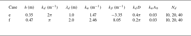


 Open access