


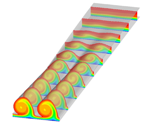



1. Introduction
Accurate prediction and effective control of the hypersonic boundary layer transition from laminar to turbulence are of great significance in the design of thermal protection systems for space vehicles. However, the transition is still an unresolved problem due to its highly nonlinear nature and sensitivity to numerous factors (Mack Reference Mack1984). In high-enthalpy boundary layers, the transition process is even more complicated due to the so-called ‘high-temperature (real-gas) effects’ (see Anderson Reference Anderson2006). Specifically, the high temperature behind shocks and in the boundary layer excites molecular vibrational/electronic energy and causes chemical dissociation and even ionization. These thermal and chemical processes invalidate the calorically perfect gas (CPG) assumption. Consequently, new physical models are required to simulate the thermochemical non-equilibrium (TCNE) flow (Gupta, Yos & Thompson Reference Gupta, Yos and Thompson1990). These TCNE effects inevitably influence the boundary layer transition process.
For practical configurations, multiple flow instabilities exist in different regions, including the leading-edge instability, streamwise instability, centrifugal instability, cross-flow instability and so on (Reed & Saric Reference Reed and Saric1989). Here the cross-flow is a secondary flow within the boundary layer due to the imbalance between the pressure gradient and centrifugal force perpendicular to the potential flow. The cross-flow profile is subject to an inviscid instability because of the existence of inflection points (Mack Reference Mack1984). The cross-flow instability is vital in many different three-dimensional boundary layers, such as the flows over swept wings, yawed cones and asymmetric bodies, making it attractive to many researchers.
The frequency of the most unstable cross-flow mode is generally much lower than those of the streamwise instability modes, such as the Tollmien–Schlichting mode and the second mode (Mack Reference Mack1984). The mode of zero frequency is called the stationary cross-flow mode, while the unsteady one is the travelling cross-flow mode. Poll (Reference Poll1985) observed both stationary and travelling cross-flow disturbances in a swept-cylinder experiment. They have different behaviours in the receptivity mechanism and disturbance evolution. For incompressible boundary layers, both theoretical and experimental researches reveal that the stationary cross-flow mode is more receptive to surface roughness and low-amplitude free-stream turbulence, while the travelling one is more receptive to the free-stream turbulence at high amplitude (Schrader, Brandt & Henningson Reference Schrader, Brandt and Henningson2009; Kurian, Fransson & Alfredsson Reference Kurian, Fransson and Alfredsson2011). Experimental measurements of the receptivity coefficients were reported by Borodulin et al. (Reference Borodulin, Ivanov, Kachanov and Roschektaev2013). When the mode disturbance at small amplitude is excited, it experiences linear and nonlinear evolution further downstream. Substantial experimental efforts were made in this area by Bippes and co-workers (see the review of Bippes Reference Bippes1999) at DLR, as well as Saric and co-workers (see the review of Saric, Reed & White Reference Saric, Reed and White2003) at ASU in the 1980s and 1990s. Müller & Bippes (Reference Müller and Bippes1989) observed the saturation of cross-flow vortex due to nonlinear effects downstream of the linear growth region. Furthermore, Kohama, Saric & Hoos (Reference Kohama, Saric and Hoos1991) (also Poll Reference Poll1985) reported the existence of high-frequency waves prior to transition in their swept-wing experiments. The frequencies of these waves are an order of magnitude higher than that of the most unstable travelling wave. They are attributed to the secondary instability of stationary cross-flow vortices where the distorted base flow has very strong and inflectional shear layers. The growth rates of the secondary instability modes are much larger than those of the primary modes, resulting in ‘explosive growth’ of disturbances and then rapid breakdown to turbulence. Detailed secondary instability measurements of stationary cross-flow vortices were provided by White & Saric (Reference White and Saric2005) for a swept-wing model. A type-I mode, which lives on the outer side of the upwelling zone (with the inner side underneath the vortex) of the vortex, was the highest-amplitude mode in nearly all cases. In comparison, a type-II mode was clearly detected only in the case with the highest free-stream Reynolds number, located on top of the vortex. Here the classification of unstable secondary instability modes is based on their production mechanisms (Malik et al. Reference Malik, Li, Choudhari and Chang1999). Type-I, or  $z$, modes are mainly produced by the spanwise gradients of the streamwise flow (i.e. $\partial U/\partial z$), while type-II, or $y$, modes are primarily driven by the wall-normal gradients (i.e. $\partial U/\partial y$). Recently, high-resolution experimental techniques were used by Serpieri & Kotsonis (Reference Serpieri and Kotsonis2016) to identify and quantify the type-I, type-II and low-frequency type-III modes. The last was located at the inner side of the upwelling region and resulted from the interaction between stationary and travelling cross-flow vortices.
A number of numerical techniques were also successfully applied to investigate the cross-flow instability. Malik, Li & Chang (Reference Malik, Li and Chang1994) utilized the nonlinear parabolized stability equations (NPSE) method to calculate the nonlinear evolution of stationary cross-flow vortices in a swept Hiemenz flow. The typical phenomena reported in the experiment, such as half-mushroom structures and vortex doubling, were captured and further analysed. Haynes & Reed (Reference Haynes and Reed2000) performed a detailed comparison between the results from the ASU experiment and linear/nonlinear instability solvers. Linear stability theory (LST) and NPSE were shown to reasonably predict the linear growth and nonlinear saturation of stationary cross-flow disturbance. Different from the streamwise marching procedure in NPSE, Koch et al. (Reference Koch, Bertolotti, Stolte and Hein2000) regarded the saturated cross-flow vortex as a nonlinear equilibrium solution of the system, and directly solved the equations. In following research, Koch (Reference Koch2002) (also Wassermann & Kloker Reference Wassermann and Kloker2002) confirmed that the primary and secondary cross-flow instabilities were both convective. This physical behaviour supports the reasonability of the streamwise marching procedure in PSE. Based on the base flow distorted by the cross-flow vortices, various numerical tools can be employed to calculate their secondary instabilities. These tools include the classic Floquet-based secondary instability theory (SIT) (Janke & Balakumar Reference Janke and Balakumar2000; Koch et al. Reference Koch, Bertolotti, Stolte and Hein2000), biglobal stability analyses (Malik et al. Reference Malik, Li, Choudhari and Chang1999; Theofilis Reference Theofilis2011) and direct numerical simulations (DNS) (Högberg & Henningson Reference Högberg and Henningson1998; Wassermann & Kloker Reference Wassermann and Kloker2003). Bonfigli & Kloker (Reference Bonfigli and Kloker2007) performed comparisons between the secondary instability results from DNS and SIT. The growth rate from SIT was found to be sensitive to the distorted base flow. When the base flow was from DNS, SIT gave a basically consistent growth rate. Their results also confirmed the accuracy of the extended Gaster transformation (Malik et al. Reference Malik, Li, Choudhari and Chang1999; Koch et al. Reference Koch, Bertolotti, Stolte and Hein2000), which converted the temporal growth rate of secondary instability mode to the spatial growth rate. Consequently, the  $N$ factor envelope of secondary instability modes was obtained for transition prediction. As another approach to obtain an accurate mean flow, Groot et al. (Reference Groot, Serpieri, Pinna and Kotsonis2018) conducted their biglobal analyses with the base flow directly from high-resolution experimental measurements. High-frequency type-I and type-II modes were found ultimately responsible for the turbulent breakdown. Using biglobal analyses, Li et al. (Reference Li, Choudhari, Chang and White2010, Reference Li, Choudhari, Duan and Chang2014) investigated the secondary instability of stationary and travelling cross-flow vortices. In their case, SIT somewhat overestimated the growth rate as it neglected the flow non-parallelism.
The cross-flow instability in hypersonic flows has received increasing attention in recent years, especially with the implementation of the Hypersonic International Flight Research Experimentation (HIFiRE) project (see Kimmel et al. Reference Kimmel, Adamczak, Borg, Jewell, Juliano, Stanfield and Berger2019). Two configurations, HIFiRE-1 (yawed circular cone) and HIFiRE-5 (elliptical cone), were specially designed for transition study. The boundary layers over these two models are subject to strong cross-flow instability. For the yawed circular cone, Kocian et al. (Reference Kocian, Moyes, Reed, Craig, Saric, Schneider and Edelman2019) reviewed elaborately the combined experimental and computational efforts on the cases at free-stream Mach numbers of around 6. The experimental facilities included two quiet wind tunnels, and the numerical techniques were NPSE and biglobal analyses. The results from experiments and computations were satisfactorily cross-validated with each other. Furthermore, it was suggested that different from the streamwise instability where the new second mode appeared and dominated in hypersonic flows, the cross-flow instability displayed some fundamental similarities between the cases of low- and high-speed flows. In other words, the cross-flow instability mechanisms were insensitive to the Mach number. Nevertheless, some quantitative differences were also reported. One important finding was that the growth of secondary instability modes in their cases was not as ‘explosive’ and was even somewhat saturated downstream (see Craig & Saric Reference Craig and Saric2016). Another finding was that the frequency of the secondary instability mode could be close to that of the second mode, so there could be a possible new type of modal interaction (Li et al. Reference Li, Choudhari, Paredes and Duan2016). The PSE and biglobal analyses were adopted by Moyes et al. (Reference Moyes, Paredes, Kocian and Reed2017) to investigate different secondary instability modes according to the experimental set-up. Unstable travelling cross-flow mode and the second mode were also recognized. Furthermore, the low- and high-frequency disturbances in the experiment by Craig & Saric (Reference Craig and Saric2016) were identified as travelling cross-flow mode and type-I mode, while in the experiment by Ward, Henderson & Schneider (Reference Ward, Henderson and Schneider2015) the second mode and type-II mode were also identified. The biglobal analyses results of Li et al. (Reference Li, Choudhari, Paredes and Duan2016) showed that only one mode of secondary cross-flow instability reached a comparable  $N$ factor with the second mode along the geometry considered.
Paredes et al. (Reference Paredes, Gosse, Theofilis and Kimmel2016) performed biglobal stability analyses of the HIFiRE-5 elliptical cone flows at a free-stream Mach number of 7.45. They identified four types of instabilities: the second, attachment-line, cross-flow and centreline (classified as a shear-layer instability) modes. The centreline modes were the strongest candidates leading to transition, while the cross-flow mode existed over most of the cone surface away from symmetry planes. On the HIFiRE-5b flight geometry, Moyes et al. (Reference Moyes, Kocian, Mullen and Reed2018) found that when stationary cross-flow vortices saturated, both type-I and type-II modes grew, but the second mode quickly decayed. Furthermore, they noticed a correlation between the neutral point of secondary instability and the transition onset. Therefore, the combination of NPSE and biglobal analyses could be used for transition prediction. In reverse, the initial disturbance amplitude could be determined using experimentally measured transition onset. Some DNS results for the HIFiRE-5 configuration were reported by Dinzl & Candler (Reference Dinzl and Candler2017) for the evolution of stationary cross-flow vortices. Recently, combined NPSE, SIT and DNS investigations were performed by Xu et al. (Reference Xu, Chen, Liu, Dong and Fu2019) and Chen et al. (Reference Chen, Dong, Chen, Yuan and Xu2021a) for the flow over a Mach-6 swept parabola. The SIT analyses identified several secondary instability modes. For the DNS results, the type-I mode was found crucial to the breakdown, and the roles of other modes were insignificant. Vortical structures were observed along with the growth of the type-I mode, which had two counter-rotating tubes stretched along the spanwise direction. Again, no intrinsic differences were found from low-speed flows in terms of principal secondary instability modes and the formation of coherent structures. Similar flow cases were also simulated by Cerminara & Sandham (Reference Cerminara and Sandham2020) using DNS for swept and unswept cases with emphasis on the mechanisms of receptivity and breakdown.
High-temperature effects cannot be neglected in flows with high free-stream enthalpy. Malik & Anderson (Reference Malik and Anderson1991) extended LST to include high-temperature gas models. Their results for Mach-10 and Mach-15 flat-plate boundary layers demonstrated a destabilizing effect on the second-mode growth. Subsequent research also mainly focused on the streamwise instability. The LST results were capable of reproducing the transition trends concerning the second mode in high-enthalpy experiments (Johnson, Seipp & Candler Reference Johnson, Seipp and Candler1998; MacLean et al. Reference MacLean, Mundy, Wadhams, Holden, Johnson and Candler2007). Furthermore, two influence paths were concluded for the second-mode growth. On the one hand, the second mode could become destabilized at a higher frequency as the TCNE boundary layer was cooler and thinner than the CPG flow. On the other hand, the second mode could be stabilized due to the energy relaxation and endothermic reactions that the disturbance experienced (Bertolotti Reference Bertolotti1998; Johnson et al. Reference Johnson, Seipp and Candler1998; Bitter & Shepherd Reference Bitter and Shepherd2015). The relative strength of these two competing effects could be estimated based on their Damköhler numbers (the ratio of the thermochemical process time scales to the flow time scale). Miró Miró et al. (Reference Miró Miró, Beyak, Pinna and Reed2019) provided a comprehensive comparison among the LST results using different high-temperature gas models. In addition to LST, linear PSE was developed by Chang, Vinh & Malik (Reference Chang, Vinh and Malik1997) for chemically non-equilibrium flows. This method was also embedded in the software LASTRAC of NASA (Kline, Chang & Li Reference Kline, Chang and Li2018) and VESTA of VKI (Zanus, Miró Miró & Pinna Reference Zanus, Miró Miró and Pinna2019). Utilizing these tools, the transition  $N$ factors of high-enthalpy flows were obtained after correlating with the experiment results (Germain & Hornung Reference Germain and Hornung1997; Malik Reference Malik2003; Grossir, Pinna & Chazot Reference Grossir, Pinna and Chazot2019). Recently, the NPSE and SIT methods were extended to include TCNE models for two-dimensional high-enthalpy boundary layers (Chen, Wang & Fu Reference Chen, Wang and Fu2021c). The fundamental resonance was found dominant in the secondary instability of the second mode. In addition, TCNE effects led to a larger maximum secondary-instability growth rate and corresponding azimuthal (spanwise) wavenumber. To drop most of the assumptions on flow perturbations, the DNS method was also developed to account for non-equilibrium effects (Stemmer Reference Stemmer2005; Prakash et al. Reference Prakash, Parsons, Wang and Zhong2011; Marxen et al. Reference Marxen, Magin, Shaqfeh and Iaccarino2013; Di Renzo, Fu & Urzay Reference Di Renzo, Fu and Urzay2020). The first DNS study from laminar all the way to turbulence in high-enthalpy flows was reported recently by Di Renzo & Urzay (Reference Di Renzo and Urzay2021). The main emphasis was on the flow downstream of the secondary instability region. Transitional and turbulent perturbations, as well as coherent structures, were investigated in detail.
Compared with the streamwise instability, the cross-flow instability in high-enthalpy flows has received relatively less attention. Although previous researchers suggested that the cross-flow instability mechanism was insensitive to the Mach number, the free-stream Mach numbers of their cases were limited to less than 10, and the flows were simulated under the CPG assumption. Therefore, investigations of flows at higher free-stream Mach numbers are thus required to explore the effects of TCNE. A case of a swept-wing boundary layer flow at Mach 13 was studied by Kline et al. (Reference Kline, Chang and Li2018), where the chemical non-equilibrium effects were found to stabilize the linear growth of stationary cross-flow mode on an adiabatic wall. Nevertheless, the reasons for this stabilization effect on the cross-flow mode were not clear. More importantly, the nonlinear interaction and the secondary instability of cross-flow vortices have not been explored. These are the focus of the present study. The stability analysis tools have been proven effective in previous cross-flow instability studies for hypersonic flows. They are thus employed in this study to provide systematic stability analyses for hypersonic and high-enthalpy flows.
The article is organized as follows. Section 2 describes the flow conditions and governing equations for TCNE flows. Section 3 provides the numerical methods adopted for laminar base flow calculations and instability analyses. The laminar flow and linear cross-flow instability results are studied in §§ 4 and 5. The secondary instability characteristics are discussed in § 6, and finally, the work is summarized in § 7.
2. Problem description and governing equations
The three-dimensional boundary layer over a swept wing of infinite span is considered herein. The swept wing is modelled by a swept parabolic body, which was widely adopted in previous investigations concerning cross-flow instability (see Mack & Schmid Reference Mack and Schmid2010; Xu et al. Reference Xu, Chen, Liu, Dong and Fu2019; Xi et al. Reference Xi, Ren, Wang and Fu2021). The geometry is described as
 \begin{equation} y^2 = 2 r_0 x \quad \text{and} \quad r_0 = 0.01\,{\rm m}, \end{equation}
where  $r_0$ is the radius of curvature at the leading edge. A schematic of the geometry and computational domain is provided in figure 1, where $x$,
$x$,  $y$ and $z$ are the Cartesian coordinates with the spanwise $z$ direction along the stagnation line. The sweep angle $\varLambda$ results in a non-zero spanwise velocity $W_\infty = Q_\infty \sin \varLambda$ at zero angles of attack, where $Q_\infty$ is the free-stream velocity. In terms of stability analyses, a local body-fitted coordinate $(s$–
$(s$– $\eta$– $z)$ is defined as sketched, where $s$ denotes the streamwise direction along the surface with its origin at the stagnation line and $\eta$ is the wall-normal coordinate.
Schematic of the geometry and computational domain, as well as the coordinate systems. Here  $x$,
$x$,  $y$ and $z$ are the Cartesian coordinates, and $s$,
$s$,  $\eta$ and $z$ are the local body-fitted coordinates.

The flow conditions of the benchmark case are listed in table 1, where the subscript  $\infty$ denotes free-stream values, and $T_w$ is the wall temperature. The free-stream conditions correspond to an altitude of 28 km. At such a high $Ma_\infty$, the flow temperature increases considerably behind shocks and towards the wall, where the vibrational energy and chemical dissociation become significant. A good approximation considered is the five-species model of air ( ${\rm N_2}$, ${\rm O_2}$, ${\rm NO}$, ${\rm N}$, ${\rm O}$) (Anderson Reference Anderson2006). Additional conservation equations of species mass and vibrational energy are needed as compared with CPG flows. The two-temperature model of Park (Reference Park1990) is adopted, which includes a translational/rotational temperature $T$ and a vibrational temperature $T_v$. The resulting Navier–Stokes equations for the TCNE flow take the following forms.
(i) Continuity equation:
(2.2a)(ii) Momentum equation: \begin{equation} \frac{\partial \rho}{\partial t} + \boldsymbol{\nabla} \boldsymbol{\cdot} \left(\rho \boldsymbol{u}\right) = 0. \end{equation}(2.2b)(iii) Energy equation:\begin{equation} \rho \left(\frac{\partial \boldsymbol{u}}{\partial t} + \boldsymbol{u} \boldsymbol{\cdot} \boldsymbol{\nabla} \boldsymbol{u}\right) ={-}\boldsymbol{\nabla} p + \boldsymbol{\nabla} \boldsymbol{\cdot} \left[\mu \left( {\boldsymbol{\nabla} \boldsymbol{u} + \boldsymbol{\nabla} {{\boldsymbol{u}}^{\rm T}}} \right) \right] - \frac{2}{3} \boldsymbol{\nabla} \left( \mu {\boldsymbol{\nabla} \boldsymbol{\cdot} \boldsymbol{u}} \right). \end{equation}(2.2c)(iv) Species continuity equation (species index$$\begin{gather} \rho c_{p,{t-r}} \left(\frac{\partial T}{\partial t} + \boldsymbol{u} \boldsymbol{\cdot} \boldsymbol{\nabla} T \right)- \left(\frac{\partial p}{\partial t} + \boldsymbol{u} \boldsymbol{\cdot} \boldsymbol{\nabla} p \right) = \mu \left[ \boldsymbol{\nabla} \boldsymbol{u} \boldsymbol{:} \left( {\boldsymbol{\nabla} \boldsymbol{u} + \boldsymbol{\nabla} {{\boldsymbol{u}}^{\rm T}}} \right) - \frac{2}{3} \left( {\boldsymbol{\nabla} \boldsymbol{\cdot} \boldsymbol{u}} \right)^2 \right]\nonumber\\ +\,\boldsymbol{\nabla} \boldsymbol{\cdot} \left(\kappa_{t-r} \boldsymbol{\nabla} T\right) + \sum_{m,n} \left(\rho D_{mn} c_{p,{t-r},m} \boldsymbol{\nabla} T \boldsymbol{\cdot} \boldsymbol{\nabla} Y_n\right) - Q_{t-v} - \sum_m \left(h_m \dot{\omega}_m\right). \end{gather}$$$s\in [2,5]$):
(2.2d)(v) Vibrational energy equation:\begin{equation} \rho \left(\frac{\partial Y_s}{\partial t} + \boldsymbol{u} \boldsymbol{\cdot} \boldsymbol{\nabla} Y_s\right) = \boldsymbol{\nabla} \boldsymbol{\cdot} \left(\sum_m {\rho D_{sm} \boldsymbol{\nabla} Y_m}\right) + \dot{\omega}_s. \end{equation}(2.2e)(vi) Equation of state:\begin{equation} \rho c_{vib} \left(\frac{\partial T_v}{\partial t} + \boldsymbol{u} \boldsymbol{\cdot} \boldsymbol{\nabla} T_v \right) = \boldsymbol{\nabla} \boldsymbol{\cdot} \left( \kappa_v \boldsymbol{\nabla} T_v\right) + \sum_{m,n} \left(\rho D_{mn} c_{{vib},m} \boldsymbol{\nabla} {T_v} \boldsymbol{\cdot} \boldsymbol{\nabla} {Y_n} \right) + Q_{t-v}. \end{equation}(2.2f)\begin{equation} p = \rho R T, \quad R = \sum_m \left(Y_m R_m\right). \end{equation}
\begin{equation} \frac{\partial \rho}{\partial t} + \boldsymbol{\nabla} \boldsymbol{\cdot} \left(\rho \boldsymbol{u}\right) = 0. \end{equation}(2.2b)(iii) Energy equation:\begin{equation} \rho \left(\frac{\partial \boldsymbol{u}}{\partial t} + \boldsymbol{u} \boldsymbol{\cdot} \boldsymbol{\nabla} \boldsymbol{u}\right) ={-}\boldsymbol{\nabla} p + \boldsymbol{\nabla} \boldsymbol{\cdot} \left[\mu \left( {\boldsymbol{\nabla} \boldsymbol{u} + \boldsymbol{\nabla} {{\boldsymbol{u}}^{\rm T}}} \right) \right] - \frac{2}{3} \boldsymbol{\nabla} \left( \mu {\boldsymbol{\nabla} \boldsymbol{\cdot} \boldsymbol{u}} \right). \end{equation}(2.2c)(iv) Species continuity equation (species index$$\begin{gather} \rho c_{p,{t-r}} \left(\frac{\partial T}{\partial t} + \boldsymbol{u} \boldsymbol{\cdot} \boldsymbol{\nabla} T \right)- \left(\frac{\partial p}{\partial t} + \boldsymbol{u} \boldsymbol{\cdot} \boldsymbol{\nabla} p \right) = \mu \left[ \boldsymbol{\nabla} \boldsymbol{u} \boldsymbol{:} \left( {\boldsymbol{\nabla} \boldsymbol{u} + \boldsymbol{\nabla} {{\boldsymbol{u}}^{\rm T}}} \right) - \frac{2}{3} \left( {\boldsymbol{\nabla} \boldsymbol{\cdot} \boldsymbol{u}} \right)^2 \right]\nonumber\\ +\,\boldsymbol{\nabla} \boldsymbol{\cdot} \left(\kappa_{t-r} \boldsymbol{\nabla} T\right) + \sum_{m,n} \left(\rho D_{mn} c_{p,{t-r},m} \boldsymbol{\nabla} T \boldsymbol{\cdot} \boldsymbol{\nabla} Y_n\right) - Q_{t-v} - \sum_m \left(h_m \dot{\omega}_m\right). \end{gather}$$$s\in [2,5]$):
(2.2d)(v) Vibrational energy equation:\begin{equation} \rho \left(\frac{\partial Y_s}{\partial t} + \boldsymbol{u} \boldsymbol{\cdot} \boldsymbol{\nabla} Y_s\right) = \boldsymbol{\nabla} \boldsymbol{\cdot} \left(\sum_m {\rho D_{sm} \boldsymbol{\nabla} Y_m}\right) + \dot{\omega}_s. \end{equation}(2.2e)(vi) Equation of state:\begin{equation} \rho c_{vib} \left(\frac{\partial T_v}{\partial t} + \boldsymbol{u} \boldsymbol{\cdot} \boldsymbol{\nabla} T_v \right) = \boldsymbol{\nabla} \boldsymbol{\cdot} \left( \kappa_v \boldsymbol{\nabla} T_v\right) + \sum_{m,n} \left(\rho D_{mn} c_{{vib},m} \boldsymbol{\nabla} {T_v} \boldsymbol{\cdot} \boldsymbol{\nabla} {Y_n} \right) + Q_{t-v}. \end{equation}(2.2f)\begin{equation} p = \rho R T, \quad R = \sum_m \left(Y_m R_m\right). \end{equation}


Here  $\rho$ and $p$ are the density and pressure; $\boldsymbol {u} = [u,v,w]^\mathrm {T}$ is the velocity vector; $c_{p,{t-r}}$ and $c_{vib}=\partial e_v/\partial T_v$ are the translational–rotational and vibrational components of specific heat, respectively, where $e_v$ denotes the specific vibrational energy; the species mass fraction $Y_s=\rho _s/\rho$ and $R_s$ is the species gas constant; $h_s$ denotes the species specific enthalpy; and the species vibrational energy is calculated using the characteristic vibrational temperature (Miró Miró et al. Reference Miró Miró, Pinna, Beyak, Barbante and Reed2018).
Flow conditions of Mach-16 flow over a swept parabola.

The mixture's viscosity  $\mu$ and thermal conductivity $\kappa _{t-r}$ and $\kappa _v$ are calculated through the relations from Gupta et al. (Reference Gupta, Yos and Thompson1990), which are as accurate as the solution of the first-order Chapman–Enskog approximation in the absence of ions (Bottin et al. Reference Bottin, Abeele, Magin and Rini2006). The molecular collision integrals required in the relations are evaluated from the curve fits of Capitelli et al. (Reference Capitelli, Gorse, Longo and Giordano2000). The mass diffusion coefficient $\rho D_{sm}$ is associated with $\mu$ through a constant Schmidt number $Sc=0.5$. Miró Miró et al. (Reference Miró Miró, Pinna, Beyak, Barbante and Reed2018, Reference Miró Miró, Beyak, Pinna and Reed2019) concluded that the use of different mass-diffusion models or a moderate variation of $Sc$ had small influences on the boundary layer instabilities. The source terms $Q_{t-v}$ and $\dot {\omega }_s$ describe the finite-rate energy relaxation and chemical reactions, respectively. The energy relaxation between transitional and vibrational components is modelled using the Landau–Teller equation (Park Reference Park1990). Five chemical reactions among the five species are considered here:
 \begin{equation} \left. \begin{aligned}
& R_1: \quad {\text{N}_2} + M \quad\leftrightarrow \quad
2{\text{N}} + M, \\ & R_2: \quad {\text{O}_2} + M
\quad\leftrightarrow \quad 2{\text{O}} + M, \\ & R_3: \quad
{\text{NO}} + M \quad\leftrightarrow \ \ \, {\text{N}} +
{\text{O}} + M, \\ & R_4: \quad {\text{N}_2} + {\text{O}}
\quad\leftrightarrow \quad {\text{NO}} + {\text{N}}, \\ &
R_5: \quad {\text{NO}} + {\text{O}} \quad\leftrightarrow
\ \ \, {{\text{O}_2}} + {\text{N}},
\end{aligned} \right\}
\end{equation}
\begin{equation} \left. \begin{aligned}
& R_1: \quad {\text{N}_2} + M \quad\leftrightarrow \quad
2{\text{N}} + M, \\ & R_2: \quad {\text{O}_2} + M
\quad\leftrightarrow \quad 2{\text{O}} + M, \\ & R_3: \quad
{\text{NO}} + M \quad\leftrightarrow \ \ \, {\text{N}} +
{\text{O}} + M, \\ & R_4: \quad {\text{N}_2} + {\text{O}}
\quad\leftrightarrow \quad {\text{NO}} + {\text{N}}, \\ &
R_5: \quad {\text{NO}} + {\text{O}} \quad\leftrightarrow
\ \ \, {{\text{O}_2}} + {\text{N}},
\end{aligned} \right\}
\end{equation}
where  $M$ is a third body. The chemical equilibrium constants are calculated based on the species Gibbs free energy fitted by McBride, Zehe & Gordon (Reference McBride, Zehe and Gordon2002). The forward reaction constants are from the relations of Park, Jaffe & Partridge (Reference Park, Jaffe and Partridge2001).
The ten basic variables of (2.2) are  ${\boldsymbol q} = [\rho,u,v,w,T,Y_s,T_v]$ with $s\in [2,5]$. Hence (2.2) is expressed in an operator form as
 \begin{equation} \mathscr{N}\left({\boldsymbol q}\right) = \boldsymbol{S}\left({\boldsymbol q}\right), \end{equation}
where the operator  $\mathscr {N}$ includes unsteady, convection and diffusion terms, while $\boldsymbol {S}$ denotes the TCNE source term related to $\dot {\omega }_s$ and $Q_{t-v}$. The combination of $\rho$ and four $Y_s$, rather than five $\rho _s$, is selected as the basic variables here because once $\boldsymbol {S}$ is set to $\boldsymbol {0}$, $Y_s$ and $T_v$ are constants throughout the flow field under homogeneous boundary conditions, then (2.2) reduces to the same form as that for CPG flows: $\mathscr {N}({\boldsymbol q}) = \boldsymbol {0}$.
3. Numerical methods
3.1. Laminar flow solver
A steady laminar flow is required prior to stability analyses. In this work, (2.2) is solved in Cartesian coordinates through a fifth-order shock-fitting solver developed by Chen & Fu (Reference Chen and Fu2020). Two implicit time-marching schemes are utilized for efficiency increase, including GMRES (generalized minimal residual) and line relaxation methods. As the swept body is of infinite span, the flow is assumed to be uniform in the spanwise direction. The boundary conditions at the wall are no-slip, isothermal or adiabatic, and non-catalytic, i.e.  $(\partial Y_s/\partial \eta )_w=0$. In the far field, the boundary is located at the shock, and the post-shock parameters are obtained from the Rankine–Hugoniot relation. A symmetry condition is imposed at the boundary of $s=0$. A non-reflecting boundary condition is adopted for the outflow boundary based on characteristic variables.
Sufficient grid points of 401 are used in the wall-normal direction to ensure grid independence (see supplementary material available at https://doi.org/10.1017/jfm.2022.607 for details). In the streamwise direction, the grid density required for a converged laminar flow is lower than that for NPSE calculations, so it is determined by the latter. At most, around 40 points are distributed within one streamwise wavelength of disturbance mode.
3.2. Linear instability theory and parabolized stability analysis
Here LST and PSE are used to efficiently calculate the linear and nonlinear growth of the cross-flow disturbance. Their frameworks are briefly described below as widely used techniques (see Herbert Reference Herbert1997). The variable  $\boldsymbol {q}$ is decomposed into a steady laminar part $\bar {\boldsymbol q}$ and a disturbed part $\tilde {\boldsymbol q}$. Here $\bar {\boldsymbol q} = [ {\bar {\rho },\bar {U},\bar {V},\bar {W},\bar {T},\bar {Y}_s,\bar {T}_v} ]$ is the laminar flow solution, and $\tilde {\boldsymbol q} = [{\tilde {\rho },\tilde {u},\tilde {v},\tilde {w},\tilde {T},\tilde {Y}_s,\tilde {T}_v}]$ is the disturbance. The disturbance governing equation is written as
 \begin{equation}
\mathscr{N} \left(\bar{\boldsymbol q} + \tilde{\boldsymbol
q}\right) - \mathscr{N} \left(\bar{\boldsymbol q}\right) =
\boldsymbol{S}\left(\bar{\boldsymbol q} +
\tilde{\boldsymbol q}\right) -
\boldsymbol{S}\left(\bar{\boldsymbol q}\right).
\end{equation}
\begin{equation}
\mathscr{N} \left(\bar{\boldsymbol q} + \tilde{\boldsymbol
q}\right) - \mathscr{N} \left(\bar{\boldsymbol q}\right) =
\boldsymbol{S}\left(\bar{\boldsymbol q} +
\tilde{\boldsymbol q}\right) -
\boldsymbol{S}\left(\bar{\boldsymbol q}\right).
\end{equation}
The expanded matrix form of (3.1) in the ( $s$–
$s$– $\eta$– $z$) coordinates is
 $$\begin{gather}
{{\boldsymbol{\mathsf{F}}}} \frac{\partial
\tilde{\boldsymbol q}}{\partial t} +
\frac{{{\boldsymbol{\mathsf{A}}}}}{h_1} \frac{\partial
\tilde{\boldsymbol q}}{\partial s} +
{{\boldsymbol{\mathsf{B}}}} \frac{\partial
\tilde{\boldsymbol q}}{\partial \eta} +
{{\boldsymbol{\mathsf{C}}}} \frac{\partial
\tilde{\boldsymbol q}}{\partial z} +
{{\boldsymbol{\mathsf{D}}}} \tilde{\boldsymbol q} =
\frac{{{\boldsymbol{\mathsf{H}}}}_{ss}}{h_1^2}
\frac{\partial^2 \tilde{\boldsymbol q}}{\partial s^2} +
{{\boldsymbol{\mathsf{H}}}}_{\eta\eta} \frac{\partial^2
\tilde{\boldsymbol q}}{\partial \eta^2} \nonumber\\ +\,
{{\boldsymbol{\mathsf{H}}}}_{zz} \frac{\partial^2
\tilde{\boldsymbol q}}{\partial z^2} +
\frac{{{\boldsymbol{\mathsf{H}}}}_{s\eta}}{h_1}
\frac{\partial^2 \tilde{\boldsymbol q}}{\partial s \partial
\eta} + \frac{{{\boldsymbol{\mathsf{H}}}}_{sz}}{h_1}
\frac{\partial^2 \tilde{\boldsymbol q}}{\partial s \partial
z} + {{\boldsymbol{\mathsf{H}}}}_{\eta z} \frac{\partial^2
\tilde{\boldsymbol q}}{\partial \eta \partial z} +
\boldsymbol{N}.
\end{gather}$$
$$\begin{gather}
{{\boldsymbol{\mathsf{F}}}} \frac{\partial
\tilde{\boldsymbol q}}{\partial t} +
\frac{{{\boldsymbol{\mathsf{A}}}}}{h_1} \frac{\partial
\tilde{\boldsymbol q}}{\partial s} +
{{\boldsymbol{\mathsf{B}}}} \frac{\partial
\tilde{\boldsymbol q}}{\partial \eta} +
{{\boldsymbol{\mathsf{C}}}} \frac{\partial
\tilde{\boldsymbol q}}{\partial z} +
{{\boldsymbol{\mathsf{D}}}} \tilde{\boldsymbol q} =
\frac{{{\boldsymbol{\mathsf{H}}}}_{ss}}{h_1^2}
\frac{\partial^2 \tilde{\boldsymbol q}}{\partial s^2} +
{{\boldsymbol{\mathsf{H}}}}_{\eta\eta} \frac{\partial^2
\tilde{\boldsymbol q}}{\partial \eta^2} \nonumber\\ +\,
{{\boldsymbol{\mathsf{H}}}}_{zz} \frac{\partial^2
\tilde{\boldsymbol q}}{\partial z^2} +
\frac{{{\boldsymbol{\mathsf{H}}}}_{s\eta}}{h_1}
\frac{\partial^2 \tilde{\boldsymbol q}}{\partial s \partial
\eta} + \frac{{{\boldsymbol{\mathsf{H}}}}_{sz}}{h_1}
\frac{\partial^2 \tilde{\boldsymbol q}}{\partial s \partial
z} + {{\boldsymbol{\mathsf{H}}}}_{\eta z} \frac{\partial^2
\tilde{\boldsymbol q}}{\partial \eta \partial z} +
\boldsymbol{N}.
\end{gather}$$
Here  $h_1=1+\kappa _0 \eta$ is the Lamé coefficient related to the streamwise curvature $\kappa _0$; matrices ${{\boldsymbol{\mathsf{F}}}}$, ${{\boldsymbol{\mathsf{A}}}}$, ${{\boldsymbol{\mathsf{B}}}}$, ${{\boldsymbol{\mathsf{C}}}}$, ${{\boldsymbol{\mathsf{D}}}}$ and ${{\boldsymbol{\mathsf{H}}}}$ are all $10 \times 10$ matrices just dependent on $\bar {\boldsymbol q}$; and $\boldsymbol {N}$ represents the nonlinear term. The expressions of these matrix coefficients are very elaborate, especially in TCNE flows, and the software MAPLE is thus employed to ensure correctness. The following Fourier decomposition of a disturbance is introduced:
 \begin{equation} \tilde{\boldsymbol{q}} \left( {s,\eta,z,t} \right) = { \sum_{m={-}M_{max}}^{M_{max}}} {\sum_{n={-}N_{max}}^{N_{max}}} {\hat{\boldsymbol{q}}_{mn} \left( {s,\eta} \right)\exp \left[ {\mathrm{i} \left(\int_{s_0}^s {\alpha_{mn} \left( s \right)\,\mathrm{d} s} + n \beta z - m \omega t \right)} \right]}, \end{equation}
where  $M_{max}$ and $N_{max}$ represent one-half of the number of modes kept in the truncated Fourier series; $s_0$ is the computational onset; $\omega$ and $\beta$ are the specified circular frequency and spanwise wavenumber, respectively; $\alpha _{mn}=\alpha _{mn,r}+\mathrm {i}\alpha _{mn,i}$ is the complex streamwise wavenumber; and $\hat {\boldsymbol {q}}_{mn}$ stands for the shape function. A phase velocity is defined as $c_{mn,r} = {m\omega }/{[\alpha _{mn,r}^2+(n\beta )^2]^{1/2}}$. For brevity, a notation ( $m$,
$m$,  $n$) is introduced for the mode with a circular frequency of $m\omega$ and a spanwise wavenumber of $n\beta$. Mode (0, 0) is also called mean flow distortion, as a modification to the laminar flow after temporal and spanwise average.
The PSE for each mode takes the following form:
 \begin{align}
\hat{{{\boldsymbol{\mathsf{A}}}}}_{mn} \frac{\partial
\hat{\boldsymbol q}_{mn}}{\partial s} ={-}\left(
\hat{{{\boldsymbol{\mathsf{D}}}}}_{mn} {\hat{\boldsymbol
q}}_{mn} + \hat{{{\boldsymbol{\mathsf{B}}}}}_{mn}
\frac{\partial \hat{\boldsymbol q}_{mn}}{\partial \eta} +
\hat{{{\boldsymbol{\mathsf{C}}}}}_{mn} \frac{\partial^2
\hat{\boldsymbol q}_{mn}}{\partial \eta^2} \right) +
\hat{\boldsymbol N}_{mn} \exp {\left(-\mathrm{i}
\int_{s_0}^{s} \alpha_{mn}\,\mathrm{d} s \right)},
\end{align}
\begin{align}
\hat{{{\boldsymbol{\mathsf{A}}}}}_{mn} \frac{\partial
\hat{\boldsymbol q}_{mn}}{\partial s} ={-}\left(
\hat{{{\boldsymbol{\mathsf{D}}}}}_{mn} {\hat{\boldsymbol
q}}_{mn} + \hat{{{\boldsymbol{\mathsf{B}}}}}_{mn}
\frac{\partial \hat{\boldsymbol q}_{mn}}{\partial \eta} +
\hat{{{\boldsymbol{\mathsf{C}}}}}_{mn} \frac{\partial^2
\hat{\boldsymbol q}_{mn}}{\partial \eta^2} \right) +
\hat{\boldsymbol N}_{mn} \exp {\left(-\mathrm{i}
\int_{s_0}^{s} \alpha_{mn}\,\mathrm{d} s \right)},
\end{align}
where the matrix coefficients are functions of  $\alpha _{mn}$, $m\omega$, $n\beta$ and the matrices in (3.2), and $\hat {\boldsymbol {N}}_{mn}$ is the Fourier component of $\boldsymbol {N}$ and acts as a nonlinear forcing term. For LST, the nonlinear term is neglected and the flow is further assumed to be locally parallel, i.e. $\partial /\partial s = 0$. Hence the base wall-normal velocity is also assumed zero from the continuity equation. As a result, an eigenvalue problem is established for each Fourier mode (Malik Reference Malik1990). For PSE analysis, (3.4) is solved through a streamwise marching procedure. The auxiliary condition adopted to determine $\alpha _{mn}$ is based on the disturbance kinetic energy. The wall-normal discretization uses the Chebyshev collocation point method and the streamwise one uses the Euler scheme. In addition, a relaxation factor is introduced to improve numerical robustness at large amplitudes of harmonic waves (Zhao et al. Reference Zhao, Zhang, Liu and Luo2016). The disturbance boundary conditions at the wall are consistent with those for laminar flow:
 \begin{align}
\text{At }\eta=0:\enspace \hat{u}_{mn} = \hat{v}_{mn} =
\hat{w}_{mn} = \frac{\partial \hat{Y}_{s,mn}}{\partial
\eta} = 0,\enspace \left\{\begin{array}{@{}ll} \hat{T}_{mn} =
\hat{T}_{v,mn} = 0, & \text{if isothermal},\\
\dfrac{\partial \hat{T}_{mn}}{\partial \eta} =
\dfrac{\partial \hat{T}_{v,mn}}{\partial \eta} = 0, &
\text{if adiabatic}. \end{array} \right.
\end{align}
\begin{align}
\text{At }\eta=0:\enspace \hat{u}_{mn} = \hat{v}_{mn} =
\hat{w}_{mn} = \frac{\partial \hat{Y}_{s,mn}}{\partial
\eta} = 0,\enspace \left\{\begin{array}{@{}ll} \hat{T}_{mn} =
\hat{T}_{v,mn} = 0, & \text{if isothermal},\\
\dfrac{\partial \hat{T}_{mn}}{\partial \eta} =
\dfrac{\partial \hat{T}_{v,mn}}{\partial \eta} = 0, &
\text{if adiabatic}. \end{array} \right.
\end{align}
The  $\hat {\rho }_{mn}$ at the wall is solved through the disturbed continuity equation. For the boundary conditions at the shock, the disturbed Rankine–Hugoniot relation is solved to account for the shock–disturbance interaction (Chang et al. Reference Chang, Vinh and Malik1997).
The present PSE solver for TCNE flows has been verified with the DNS data in the authors’ previous works (see Chen, Wang & Fu Reference Chen, Wang and Fu2021b,Reference Chen, Wang and Fuc). Comparisons with the existing results of cross-flow instability cases are provided in the supplementary material.
3.3. Secondary instability analysis
Large-amplitude cross-flow vortices are subject to various types of high-frequency instabilities. The SIT can be used to obtain the disturbance characteristics by solving the instability equation on the distorted base flow. For stationary cross-flow vortices, the NPSE solution is written as
 \begin{equation} \tilde{\boldsymbol q}_{NPSE} \left( {s,\eta,z} \right) = \sum_{n} {A_{0n} \hat{\boldsymbol{q}}_{0n} \exp \left[ {{\mathrm i} n \left(\int_{s_0}^s {\alpha_r\,\mathrm{d} s} + \beta z \right)} \right]}, \end{equation}
where  $A_{0n}$ is the mode's amplitude and $\alpha _r$ stands for the real part of the fundamental wavenumber. Therefore, the distorted base flow is $\bar {\boldsymbol {q}}^\prime = \bar {\boldsymbol {q}} + \tilde {\boldsymbol q}_{NPSE}$, and the secondary instability disturbance to be solved is $\tilde {\boldsymbol q}_{{sd}}$. The exponent in (3.6) depends on two coordinates, so a coordinate transformation is introduced to make the exponent one-coordinate-dependent. The wave front $z_r=z_r(s_r)$ is
 \begin{equation} z_r = \int_{s_0}^{s_r} {\tan \theta_2\,\mathrm{d} s} + z_0, \quad \tan \theta_2 ={-}\frac{\alpha_r}{\beta}, \end{equation}
where  $\theta _2$ is the slope angle and $z_0$ is a reference point. Physically, the tangent line indicates the direction of the cross-flow vortex axis, and thus a local vortex-oriented coordinate $(s_2$– $\eta _2$– $z_2)$, with its origin at $(s=s_r,\eta =0,z=z_r)$, can then be defined as
 \begin{equation} \left. \begin{aligned} s_2 & = \left(z - z_r\right) \sin \theta_2 + \left(s - s_r\right) \cos \theta_2,\\ z_2 & = \left(z - z_r\right) \cos \theta_2 - \left(s - s_r\right) \sin \theta_2,\\ \eta_2 & = \eta . \end{aligned} \right\} \end{equation}
A schematic of this vortex-oriented coordinate is provided in figure 2. A locally parallel flow is further assumed in SIT, such that at a given location  $s=s_r$, the $s$-derivatives of $A_{0n} \hat {\boldsymbol {q}}_{0n}$ are much smaller than the $\eta$-derivatives, so the $s$-dependence of $A_{0n}$, $\alpha _r$ and $\hat {\boldsymbol {q}}_{0n}$ is neglected in a small region near $s_r$ (Koch et al. Reference Koch, Bertolotti, Stolte and Hein2000; Bonfigli & Kloker Reference Bonfigli and Kloker2007). This is reasonable because strong secondary instability usually occurs where the cross-flow vortices are saturated (see § 6). Consequently, the disturbance in (3.6) near $s=s_r$ is rewritten as
 \begin{equation} \tilde{\boldsymbol q}_{NPSE} \left( {\eta_2,z_2} \right) = \sum_{n} {A_{0n} \hat{\boldsymbol{q}}_{0n} \left( {\eta_2} \right) \exp \left( {{\mathrm i} n \beta_2 z_2} \right)}, \end{equation}
where  $\beta _2=\beta /\cos \theta _2$ is the $z_2$-direction wavenumber. As a result of the locally-parallel-flow assumption, $\tilde {\boldsymbol q}_{NPSE}$ is explicitly independent of $s_2$ and periodic in the $z_2$ direction.
Definition of the vortex-oriented coordinates.

The velocities in the vortex-oriented coordinates are
 \begin{equation} u_2 = w \sin \theta_2 + u \cos \theta_2, \quad w_2 = w \cos \theta_2 - u \sin \theta_2, \quad v_2 = v. \end{equation}
Therefore, the variable in SIT is  ${\boldsymbol q}_2 = [\rho,u_2,v_2,w_2,T,Y_s,T_v]$, and the base flow distorted by the stationary cross-flow vortex is
 \begin{equation} \bar{\boldsymbol{q}}_2^\prime \left( {\eta_2,z_2} \right) = \bar{\boldsymbol{q}}_2\left(\eta_2\right) + \sum_{n} {A_{0n} \hat{\boldsymbol{q}}_{2,0n} \left(\eta_2\right) \exp \left( {\mathrm i} n \beta_2 z_2 \right)}. \end{equation}
Similarly, the disturbance to be solved is replaced as  $\tilde {\boldsymbol q}_{2,{ sd}}$, and the governing equation is
 \begin{equation} \mathscr{N}\left(\bar{\boldsymbol{q}}_2^\prime + \tilde{\boldsymbol q}_{2,{ sd}}\right) - \mathscr{N}\left(\bar{\boldsymbol{q}}_2^\prime\right) = \boldsymbol{S}\left(\bar{\boldsymbol{q}}_2^\prime + \tilde{\boldsymbol q}_{2,{ sd}}\right) - \boldsymbol{S}\left(\bar{\boldsymbol{q}}_2^\prime\right), \end{equation}
which can be expanded into a similar form to (3.2).
Equation (3.12) is solved through the Floquet theory (see Herbert Reference Herbert1988), so a temporal-mode solution is written as
 \begin{equation} \tilde{\boldsymbol q}_{2,{ sd}} = \varepsilon \left\{\sum_{n={-}N_{sd}}^{N_{sd}} {\hat{\boldsymbol q}_{2,n} \left(\eta_2\right) \exp \left[ {\mathrm{i}\left(n + \sigma_d\right) \beta_2 z_2} \right]}\right\} \exp \left({\omega_s t + \mathrm{i} \alpha_s s_2}\right), \end{equation}
where  $\varepsilon$ is the mode amplitude, $\omega _s = \omega _{s,r} + \mathrm {i} \omega _{s,i}$ the temporal characteristic exponent, $\omega _{s,r}$ the mode growth rate and $\omega _{s,i}$ the shift in the circular frequency. Also, $\sigma _d$ denotes the detuning parameter and $N_{sd}$ is the truncated orders. The corresponding phase velocity is defined as $c_{s,r}=-\omega _{s,i}/\alpha _s$. After substituting (3.11) and (3.13) into (3.12) and neglecting $O(\varepsilon ^2)$ terms, a complex eigenvalue problem is obtained:
 \begin{equation} \boldsymbol{\mathcal{A}} \hat{\boldsymbol Q} = \omega_s \boldsymbol{\mathcal{B}} \hat{\boldsymbol Q}. \end{equation}
Here  $\hat {\boldsymbol Q}$ is the global eigenvector containing all $\hat {\boldsymbol q}_{2,n}$. Matrices $\boldsymbol{\mathcal{A}}$ and $\boldsymbol{\mathcal {B}}$ are global matrices with dimensions of $[10N_y\times (2N_{sd}+1)]^2$. The boundary conditions for $\hat {\boldsymbol q}_{2,n}$ at the wall are
 \begin{equation} \text{At }\eta=0:\quad \hat{u}_{2,n} = \hat{v}_{2,n} = \hat{w}_{2,n} = \hat{T}_{n} = \hat{T}_{v,n} = \hat{Y}_{s,n} = 0. \end{equation}
The main consideration is that the frequency of the secondary cross-flow instability mode is usually high (of the order of 100 kHz; see § 6.4), so  $\hat {T}_{n}$, $\hat {T}_{v,n}$ and $\hat {Y}_{s,n}$ are forced to vanish at the wall owing to the thermal inertia of the solid body (Malik Reference Malik1990; Bitter & Shepherd Reference Bitter and Shepherd2015). The Dirichlet conditions in (3.15) are also used at the far-field boundary because $\hat {\boldsymbol q}_{2,n}$ quickly decays outside the boundary layer. The eigenvalues and eigenvectors of the large-scale matrices are solved through the same algorithm as that in LST. More details can be found in Koch et al. (Reference Koch, Bertolotti, Stolte and Hein2000) and Ren & Fu (Reference Ren and Fu2015).
4. Laminar flow results
The laminar flow field is investigated first. The flow is also calculated under the CPG assumption for comparison to clarify the effect of TCNE. Instead of Sutherland's law, the same air composition and transport models as described in § 2 are adopted for consistency. Figure 3(a) provides the laminar temperature contours in the TCNE and CPG benchmark cases around the nose region of the parabola. A noticeable difference is that the temperature in the TCNE case is much lower than that in the CPG case due to strong thermochemical processes downstream of the shock. The difference is most obvious downstream of the normal shock at  $y=0$, and the distributions of $\bar {T}$ and $\bar {T}_v$ along the streamline at $y=0$ are plotted in figure 3(b). In the CPG case, $\bar {T}$ slowly increases downstream until a sudden drop at $x>-0.23\,\textrm {mm}$ due to the specified low $T_w$. In comparison, $\bar {T}$ in the TCNE case quickly decreases downstream of the shock, and is at most 2268 K lower than that of the CPG case. As a result, the shock stand-off distance is 32 % smaller at $y=0$. The decrease of temperature in the TCNE case is accompanied by the rise of the vibrational energy and mass fractions of NO, O and N. Vibrational temperature $\bar {T}_v$ rapidly increases to over 4500 K and tends to vibrational equilibrium further downstream towards the wall. Moreover, large fractions of NO and O are produced, as shown in figure 3(c), and the minimum mass fractions of ${\rm N_2}$ and ${\rm O_2}$ are 0.737 and 0.114, respectively. Figure 4 gives the contours of $\bar {T}_v$ and $\bar {Y}_{O_2}$ around the nose region. Away from the stagnation line, $\bar {T}_v$ along with $\bar {T}$ decrease due to the fluid acceleration. Vibrational temperature $\bar {T}_v$ decreases more slowly and is higher than $\bar {T}$ in the displayed range. The dissociation of ${\rm O_2}$ mainly occurs near the wall due to local high temperature and the chemical non-equilibrium effect.
(a) Laminar temperature contours around the nose region, and the streamwise distribution of (b) temperatures and (c) species mass fractions (TCNE only) along the streamline at  $y=0$ in the TCNE and CPG benchmark cases.

Laminar flow contours around the nose region of the parabola in the TCNE benchmark case: (a) vibrational temperature and (b) mass fraction of oxygen.

The potential-flow direction is required in the calculation to obtain the cross-flow velocity. Actually, the flow outside the boundary layer is not irrotational, as will be discussed later. As  $\bar {W}$ is uniform in the inviscid-flow region, the boundary layer edge $(\eta =\delta _N)$ is determined from the profile of $\bar {W}$ with $\bar {W}(\delta _N)=0.995W_\infty$. The angle of the potential streamline is $\theta _e = \arctan (\bar {W}_e/\bar {U}_e)$, where the subscript $e$ denotes the boundary-layer-edge value at $\delta _N$. As a result, the potential-flow velocity $\bar {U}_{pl}$ and cross-flow velocity $\bar {U}_{cf}$ are
 \begin{equation} \left. \begin{aligned} \bar{U}_{pl} & = \bar{U} \cos \theta_e + \bar{W} \sin \theta_e,\\ \bar{U}_{cf} & ={-}\bar{U} \sin \theta_e + \bar{W} \cos \theta_e. \end{aligned} \right\} \end{equation}
Here  $\bar {U}_{cf}$ is basically negative under the present coordinates. The streamwise distribution of the quantities at the wall and the boundary layer edge is plotted in figure 5. The coincidence of the two wall-pressure curves in the TCNE and CPG cases indicates that the surface pressure distribution is insensitive to TCNE effects, which is basically determined by the flow outside the boundary layer. In comparison with the CPG case, $\theta _e$ in the TCNE case is roughly $2^{\circ }{-}4^{\circ }$ larger due to a smaller $\bar {U}_e$. This leads to a larger pressure gradient perpendicular to the potential-flow direction, i.e. $(\partial p_e/\partial x)\cos \theta _e$, within the boundary layer, which tends to increase the cross-flow velocity. Due to the entropy layer produced by the strong bow shock, $T_e$ is much higher than $T_\infty$, as shown in figure 5(b). As a result, $Ma_e$ is much lower than the free-stream value, different from the flows over a sharp leading edge. In both the TCNE and CPG cases, $Ma_e$ continuously increases with $s$ and is close to 5 at $s=1\,\textrm {m}$. Meanwhile, $Ma_e$ in the TCNE case is generally 0.18–0.45 higher, owing to the lower $T_e$.
Streamwise distribution of (a) wall pressure and flow direction at the boundary layer edge and of (b) edge temperature and Mach number in the TCNE and CPG cases.

The boundary layer profiles are plotted in figure 6 at two  $s$ of 0.1 and 0.5 m. As can be seen, the $\bar {U}_{pl}$ profile is less sensitive to the TCNE effects, and $\delta _N$ in the TCNE case is only slightly smaller, though the temperature is hundreds of kelvins lower. This is related to the increase of $\bar {R}$ due to the production of atoms. From ( 2.2f), the production of $\bar {R}$ and $\bar {T}$ happens to be almost unchanged by TCNE, so the density profile (not shown here) and thus the boundary layer thickness only experience slight variations. From figure 6(b), $T_w$ is lower than $T_e$, which is commonly considered, in the stability theory, as a ‘highly cooled wall’ case (Bitter & Shepherd Reference Bitter and Shepherd2015). The effects of wall cooling are discussed in § 5.2. Besides, the difference between $\bar {T}$ and $\bar {T}_v$ indicates that the flow is still in thermal non-equilibrium inside and outside the boundary layer. For chemical species, it is observed that there are still reactions outside the boundary layer due to the high temperature in the inviscid-flow region. Within the boundary layer, the mass fractions of ${\rm O_2}$ and NO are nearly unchanged in the wall-normal direction. Meanwhile, the species mass fractions at the wall vary slowly in the streamwise direction, and the TCNE effects are retained far downstream.
Boundary layer profiles at different  $s$ in the TCNE and CPG cases: (a) velocity in the potential-flow direction, (b) temperature and vibrational temperature (TCNE only) and (c) species mass fractions (TCNE only). Only $\delta _N$ in the TCNE case is labelled for clarity.

The streamwise distribution of  $U_{{cf},max}$, defined as the maximum $|\bar {U}_{cf}|$ in the wall-normal direction inside the boundary layer, is given in figure 7(a). For both cases, $U_{{cf},max}$ quickly increases from zero to the maximums at $s\approx 0.1\,\textrm {m}$, and gradually decreases further downstream. The peak of $U_{{cf},max}$ in the TCNE case is 6 % higher, but it also drops more quickly. The cross-flow Reynolds number, $Re_{{cf},e}=\rho _e U_{{cf},max} \delta _N/\mu _e$, is evaluated to be 324 at $s=0.1\,\textrm {m}$. The profiles of $\bar {U}_{cf}$ at different streamwise locations are depicted in figure 7(b,c). The curve shapes are similar at different $s$ except for the increasing boundary layer thickness. Meanwhile, $|\bar {U}_{cf}|$ tends to increase outside the boundary layer in both the TCNE and CPG cases, which means that the flow outside the boundary layer is rotational, and the velocity curl is mainly from $\partial \bar {U}_{cf}/\partial \eta$. This can be interpreted through the Crocco theorem, which, for CPG flows, is written as
 \begin{equation} \bar{T} \boldsymbol{\nabla} \bar{S} = \boldsymbol{\nabla} \bar{H} - \bar{\boldsymbol U} \times \left(\boldsymbol{\nabla} \times \bar{\boldsymbol U}\right), \end{equation}
where  $S$ and $H$ are the entropy and total enthalpy. As $\bar {H}$ is uniform outside the boundary layer crossing the shock, the curl of $\bar {\boldsymbol U}$ originates from the entropy gradient due to the curved bow shock.
(a) Streamwise distribution of the maximum cross-flow velocity, and the cross-flow velocity profiles at different  $s$ in (b) TCNE and (c) CPG cases. The four values of $s$ in (b,c) are labelled in (a) as dashed lines.

5. Linear instability results
5.1. Benchmark case results
The LST calculation is performed to determine the dominant disturbance mode. The contours of the disturbance growth rate and phase velocity in the benchmark TCNE and CPG cases are provided in figure 8 with different frequencies  $f$ and spanwise wavelengths $\lambda _z=2{\rm \pi} /\beta$. It is worth mentioning that the growth rate $-\alpha _i$ is measured in the $s$ direction. If measured in the potential-flow direction (or the cross-flow vortex orientation), then the corresponding growth rate is $-\alpha _i \cos \theta _e$ (or $-\alpha _i \cos \theta _2$). As can be seen, both stationary and travelling cross-flow modes have large growth rates, while no unstable streamwise instability modes are observed. The most unstable cross-flow mode is travelling, consistent with that in lower-speed flows (see e.g. Choudhari et al. Reference Choudhari, Li, Chang, Carpenter, Streett, Malik and Duan2013). At $s=0.2\,\textrm {m}$ in the TCNE case, the most unstable mode has $f$ of 6 kHz and $\lambda _z$ of 22 mm. The maximum phase velocity $c_r/Q_\infty$ of unstable cross-flow mode is 0.165, which is much smaller than those of Mack modes. Moreover, it is interesting to see that as marked by the blue dotted lines, the most unstable modes at each $\lambda _z$ (larger than 22 mm) all have roughly the same $c_r/Q_\infty$ of 0.0165, which is around one-tenth of the maximum $c_r/Q_\infty$ of unstable modes. This relation also holds at $s=0.8\,\textrm {m}$ and in the CPG case, though the corresponding phase velocity varies from case to case. Therefore, it seems to indicate some intrinsic similarities among the travelling cross-flow modes of different spanwise wavelengths. Downstream to $s=0.8\,\textrm {m}$, the unstable region is approximately twice as large in terms of spanwise wavelength and half in terms of frequency, compared with that at 0.2 m. Meanwhile, the maximum growth rate at $s=0.8\,\textrm {m}$ is only one third. In terms of gas models, the cross-flow mode in the TCNE case is shown to be more unstable than that in the CPG case. The ratios of the maximum growth rates between the two cases are 1.59 at $s=0.2\,\textrm {m}$ and 1.39 at $s=0.8\,\textrm {m}$.
Growth rate contours  $(-\alpha _i)$ [ $\textrm {m}^{-1}$] with frequencies and spanwise wavelengths: (a) TCNE and ${s=0.2\,\textrm {m}}$, (b) CPG and $s=0.2\,\textrm {m}$, (c) TCNE and $s=0.8\,\textrm {m}$ and (d) CPG and $s=0.8\,\textrm {m}$. The contours of phase velocities are also plotted as dashed lines. The level in red labelled ‘mc’ is the maximum $c_r/Q_\infty$ and the one in blue labelled ‘mg’ is the value of the most unstable mode.

Figure 9 plots the integrated  $N$ factors for the stationary and travelling cross-flow modes with fixed frequency and wavelength. The disturbances of $\lambda _z=40\,\textrm {mm}$ all have the largest $N$ factors at the end of the computational domain at $s=1.2\,\textrm {m}$. Although the most unstable mode in figure 8 is a travelling mode, its maximum $N$ factor at a fixed frequency is no higher than that of the stationary mode in both TCNE and CPG cases. Previous receptivity researches revealed that a stationary cross-flow mode was more receptive in flight conditions because of surface imperfections and low-amplitude free-stream disturbance (Kurian et al. Reference Kurian, Fransson and Alfredsson2011). In addition, the stationary mode here has an $N$ factor comparable with that of the travelling mode. Therefore, it is conjectured that the stationary cross-flow mode is more likely to dominate the disturbance linear growth regime in the present case. Furthermore, it is observed that TCNE has a significant destabilizing effect on both stationary and travelling cross-flow modes. In comparison with the CPG case, the maximum $N$ factors are lifted by 1.8–3.0 for the disturbance of the selected spanwise wavelengths. A parametric study is performed as discussed below to explain this destabilization effect of TCNE.
Streamwise distribution of the cross-flow mode  $N$ factors: (a) TCNE and stationary, (b) CPG and stationary, (c) TCNE and travelling and (d) CPG and travelling. The notation in each legend denotes the mode with [ $\,f$ in kHz, $\lambda _z$ in mm].

5.2. Effects of wall temperature and TCNE
Previous works suggested that TCNE influenced the primary instability mainly by modifying the laminar boundary layer profiles. For the second mode, both TCNE and wall cooling (decreasing  $T_w$) had a destabilization effect as they both decreased the flow temperature (Bitter & Shepherd Reference Bitter and Shepherd2015; Miró Miró et al. Reference Miró Miró, Beyak, Pinna and Reed2020). For the cross-flow mode, however, the effects of TCNE and wall cooling are somewhat the opposite. Contrary to the destabilization effect by TCNE as shown in figure 9, Arnal (Reference Arnal1996) found that wall cooling stabilized the cross-flow mode, the same as the first mode which is also an inflectional instability. To explain this opposite effect, we turn to focus on the parameter $T_w/T_e$ instead of $T_w$ alone, because $T_w$ usually appears in the non-dimensional form of $T_w/T_e$ in the stability equations (Mack Reference Mack1984). For wall cooling, $T_e$ is unchanged and $T_w$ decreases, so $T_w/T_e$ decreases. For the TCNE case here, $T_w$ is set equal to the CPG case but $T_e$ is lower (see figure 5), so $T_w/T_e$ does not decrease but increases. In this sense, TCNE is equivalent to wall heating in terms of $T_w/T_e$. Therefore, the results from the TCNE and wall-cooling cases both suggest that higher $T_w/T_e$ destabilizes the cross-flow mode and vice versa.
For verification, two more cases with different  $T_w$ and $T_\infty$, respectively, are calculated under the CPG model. The first case, termed the ‘hot-wall-CPG’ case, employs a higher $T_w$ of 2500 K. The second case only changes $T_\infty$ to 160 K, and also $p_\infty$ to keep $R_\infty$ unchanged, which is termed the ‘cold-fs-CPG’ case. Figure 10 gives comparisons of the laminar temperature profiles and the $N$ factors of stationary cross-flow modes. Only the mode with $\lambda _z=40\,\textrm {mm}$ is displayed, which has the largest $N$ factor in the domain for all three cases. In comparison with the benchmark case, $\bar {T}$ in the hot-wall-CPG case is higher, and $T_e$ is roughly unchanged. As a result, the maximum $N$ factor is larger, which confirms the stabilizing effect of wall cooling and also $T_w/T_e$ decreases. Comparisons between the benchmark and cold-fs-CPG cases are analysed in the same way. With $T_\infty$ decreased, $T_e$ is reduced by 780 K at $s=0.20\,\textrm {m}$ and 640 K at 0.80 m. Consequently, the stationary cross-flow mode is destabilized with the larger $T_w/T_e$. Therefore, it is concluded that increasing $T_w/T_e$, whether through increasing $T_w$ or decreasing $T_e$, destabilizes the cross-flow mode. Hence the lower $T_e$ in the TCNE case tends to increase the growth rate at the same $T_w$.
(a) Laminar temperature profiles at  $s=0.8\,\textrm {m}$ and (b) the $N$ factors of the stationary cross-flow modes ( $\lambda _z=40\,\textrm {mm}$) in the hot-wall-CPG, cold-fs-CPG and benchmark (b.m.) CPG cases.

We take a step further by calculating two more cases with adiabatic-wall conditions, termed ‘adia-TCNE’ and ‘adia-CPG’ cases, respectively. This condition results in the theoretically maximum  $T_w$ without external heat sources, and hence the maximum growth rate of the cross-flow mode. As shown in figure 11(a), $T_w$ in the adia-CPG case slowly decreases with $s$ and is close to the theoretical value away from the stagnation line. In comparison, $T_w$ in the adia-TCNE case is approximately 5000 K lower due to the intense energy relaxation and chemical reactions. Figure 11(b,c) gives the profiles of temperatures and mass fractions. In the adia-TCNE case, the flow is close to thermal equilibrium inside the boundary layer. The $\bar {Y}_{O_2}$ is less than 1 % at the wall, most of which dissociates into O. In terms of the $N$ factor shown in figure 12, the adiabatic-wall condition strongly destabilizes the cross-flow mode as expected, compared with the benchmark cases. As $T_w$ rises by over six times, this destabilization is more evident in the CPG case where the maximum $N$ factor is nearly doubled. For a comparison between the adia-TCNE and adia-CPG cases, the ratios $T_w/T_e$ from figure 11 are 2.80 and 4.36, respectively, i.e. $T_w/T_e$ in the adia-TCNE is smaller. However, different from the trend above, the $N$ factor in the adia-TCNE case is still larger, though the $N$-factor difference is narrowed due to the $T_w$ increase. Therefore, $T_w/T_e$ is not the only factor in determining whether TCNE is stabilizing or destabilizing as there are also energy relaxation and reactions inside the boundary layer. In the following, we turn to analyse the governing base flow and disturbance equations with two objectives. One is to provide more physical interpretations of the connection between the $T_w/T_e$ increase and the destabilization of cross-flow modes. The other is to find a parameter that works for both CPG and TCNE flows, and can correctly predict the stabilizing or destabilizing trend of cross-flow modes.
(a) Streamwise distribution of the wall temperatures, and the boundary layer profiles at  $s=0.8\,\textrm {m}$ of (b) temperature and (c) species mass fractions (TCNE only) in the adia-TCNE and adia-CPG cases.

Curves of  $N$ factor of the stationary cross-flow modes with different spanwise wavelengths in (a) the adia-TCNE case and (b) the adia-CPG case. The $N$ factors of mode [0, 40] in the benchmark CPG and TCNE cases are also plotted for reference.

Basically, the amplitude of the cross-flow velocity  $|\bar {U}_{cf}|$ is key to the growth rate of the cross-flow mode. The increase of $|\bar {U}_{cf}|$ is destabilizing with other factors unchanged (Reed & Saric Reference Reed and Saric1989). Meanwhile, from the momentum equation (2.2b), $\bar {U}_{cf}$ is primarily affected by the acceleration term $(\partial p_e/\partial x)\cos \theta _e/\bar {\rho }$ (see figure 5), which is related to the pressure gradient and the density. Figure 13(a) provides the cross-flow velocity profiles at $s=0.4\,\textrm {m}$ in all the six cases mentioned above. From the four CPG cases (the first four lines), a clear trend is observed that $|\bar {U}_{cf}|$ increases rapidly with the rise of $T_w/T_e$. This is reasonable because the rise of $T_w$ (the reduction of $T_e$ can be analysed in the same way) decreases $\bar {\rho }~(\sim 1/\bar {T})$ in the boundary layer. As a result, $(\partial p_e/\partial x)\cos \theta _e/\bar {\rho }$ increases, and thus $|\bar {U}_{cf}|$ rises. In short, for CPG flows, the increase of $T_w/T_e$ leads to a larger $|\bar {U}_{cf}|$, and hence a more destabilized cross-flow mode.
Profiles of (a) cross-flow velocity normalized by the free-stream velocity and (b) cross-flow Mach number in different CPG and TCNE cases at  $s=0.4\,\textrm {m}$. The numbers in parentheses in the inset are the corresponding values of $T_w/T_e$.

In the TCNE flows, the rise of  $T_w/T_e$ also results in an increase in $|\bar {U}_{cf}|$. Nevertheless, $|\bar {U}_{cf}|$ in the two TCNE cases are no higher than their CPG counterparts (b.m.-CPG and adia-CPG cases), contrary to the destabilization of TCNE effects shown above. As the cross-flow instability is an inflectional instability, the inviscid disturbance equations are adopted below to help locate critical parameters. After applying the LST assumptions, the governing inviscid equations are written as
 \begin{equation}
\left. \begin{aligned} & \mathrm{i} \left({ \alpha \bar{U}
+ \beta \bar{W} - \omega }\right) \hat{\rho} + \bar{\rho}
\left({ \mathrm{i} \alpha \hat{u} + \mathrm{i} \beta
\hat{v} + \mathrm{D}_\eta \hat{v}}\right) + \left({
\mathrm{D}_\eta \bar{\rho} }\right)\hat{v} = 0,\\ &
\mathrm{i} \bar{\rho} \left({ \alpha \bar{U} + \beta
\bar{W} - \omega }\right) \hat{u} + \bar{\rho} \left(
\mathrm{D}_\eta \bar{U} \right) \hat{v} + \mathrm{i} \alpha
\hat{p} = 0,\\ & \mathrm{i} \bar{\rho} \left({ \alpha
\bar{U} + \beta \bar{W} - \omega }\right) \hat{v} +
\mathrm{D}_\eta \hat{p} = 0,\\ & \mathrm{i} \bar{\rho}
\left({ \alpha \bar{U} + \beta \bar{W} - \omega }\right)
\hat{w} + \bar{\rho} \left( \mathrm{D}_\eta \bar{W} \right)
\hat{v} + \mathrm{i} \beta \hat{p} = 0,\\ & \bar{\rho}
\bar{c}_{p,t-r} \left[ {\mathrm{i} \left({ \alpha \bar{U} +
\beta \bar{W} - \omega }\right) \hat{T} + \left({
\mathrm{D}_\eta \bar{T} }\right) \hat{v}} \right] \\ &
\quad- \mathrm{i} \left({ \alpha \bar{U} + \beta \bar{W} -
\omega }\right) \hat{p} ={-} \left[ \sum_m \left( \bar{h}_m \hat{\omega}_m+ \hat{h}_m \bar{\omega}_m \right) + \hat{Q}_{t-v} \right],\\
& \mathrm{i} \bar{\rho} \left({ \alpha \bar{U}
+ \beta \bar{W} - \omega }\right) \hat{Y}_s + \bar{\rho}
\left({ \mathrm{D}_\eta \bar{Y}_s }\right) \hat{v} =
\hat{\omega}_s,\\
&\quad \bar{\rho} \bar{c}_{\textit{vib}} \left[
{\mathrm{i} \left({ \alpha \bar{U} + \beta \bar{W} - \omega
}\right) \hat{T}_v + \left({ \mathrm{D}_\eta \bar{T}_v
}\right) \hat{v}} \right] = \hat{Q}_{t-v},\\
& {\hat p} = \bar{R}\bar{T} \hat{\rho} + \bar{\rho}\bar{R} \hat{T} +
\bar{\rho}\bar{T} \sum_m {R_m \hat{Y}_m}, \end{aligned}
\right\}
\end{equation}
\begin{equation}
\left. \begin{aligned} & \mathrm{i} \left({ \alpha \bar{U}
+ \beta \bar{W} - \omega }\right) \hat{\rho} + \bar{\rho}
\left({ \mathrm{i} \alpha \hat{u} + \mathrm{i} \beta
\hat{v} + \mathrm{D}_\eta \hat{v}}\right) + \left({
\mathrm{D}_\eta \bar{\rho} }\right)\hat{v} = 0,\\ &
\mathrm{i} \bar{\rho} \left({ \alpha \bar{U} + \beta
\bar{W} - \omega }\right) \hat{u} + \bar{\rho} \left(
\mathrm{D}_\eta \bar{U} \right) \hat{v} + \mathrm{i} \alpha
\hat{p} = 0,\\ & \mathrm{i} \bar{\rho} \left({ \alpha
\bar{U} + \beta \bar{W} - \omega }\right) \hat{v} +
\mathrm{D}_\eta \hat{p} = 0,\\ & \mathrm{i} \bar{\rho}
\left({ \alpha \bar{U} + \beta \bar{W} - \omega }\right)
\hat{w} + \bar{\rho} \left( \mathrm{D}_\eta \bar{W} \right)
\hat{v} + \mathrm{i} \beta \hat{p} = 0,\\ & \bar{\rho}
\bar{c}_{p,t-r} \left[ {\mathrm{i} \left({ \alpha \bar{U} +
\beta \bar{W} - \omega }\right) \hat{T} + \left({
\mathrm{D}_\eta \bar{T} }\right) \hat{v}} \right] \\ &
\quad- \mathrm{i} \left({ \alpha \bar{U} + \beta \bar{W} -
\omega }\right) \hat{p} ={-} \left[ \sum_m \left( \bar{h}_m \hat{\omega}_m+ \hat{h}_m \bar{\omega}_m \right) + \hat{Q}_{t-v} \right],\\
& \mathrm{i} \bar{\rho} \left({ \alpha \bar{U}
+ \beta \bar{W} - \omega }\right) \hat{Y}_s + \bar{\rho}
\left({ \mathrm{D}_\eta \bar{Y}_s }\right) \hat{v} =
\hat{\omega}_s,\\
&\quad \bar{\rho} \bar{c}_{\textit{vib}} \left[
{\mathrm{i} \left({ \alpha \bar{U} + \beta \bar{W} - \omega
}\right) \hat{T}_v + \left({ \mathrm{D}_\eta \bar{T}_v
}\right) \hat{v}} \right] = \hat{Q}_{t-v},\\
& {\hat p} = \bar{R}\bar{T} \hat{\rho} + \bar{\rho}\bar{R} \hat{T} +
\bar{\rho}\bar{T} \sum_m {R_m \hat{Y}_m}, \end{aligned}
\right\}
\end{equation}
where  $\mathrm {D}_\eta =\mathrm {d}/\mathrm {d}\eta$ and $\hat {\omega }_s$ and $\hat {Q}_{t-v}$ are the linearized disturbances of $\dot {\omega }_s$ and $Q_{t-v}$. The applicability of (5.1) in describing the disturbance structure is further discussed in § 5.3. Following the procedures of Mack (Reference Mack1984), a second-order ordinary differential equation for $\hat {p}$ is finally arrived at from (5.1) as
 \begin{equation} \mathrm{D}_\eta^2 \hat{p} - \mathrm{D}_\eta ( \ln {\textit{Ma}}_r^2 ) \mathrm{D}_\eta \hat{p} - ( \alpha^2 + \beta^2 ) ( 1 - {\textit{Ma}}_r^2 ) \hat{p} = \hat{f}_S, \end{equation}
where  $\hat {f}_S$ is a function of $\hat {\omega }_s$ and $\hat {Q}_{t-v}$, and is absent in CPG flows. Moreover, $\hat {f}_S$ was shown to have minor effects on the second-mode instability (Bitter & Shepherd Reference Bitter and Shepherd2015; Chen et al. Reference Chen, Wang and Fu2021b). The most important parameter in (5.2) is the well-known relative Mach number of disturbance:
 \begin{equation} {\textit{Ma}}_r = \frac{\alpha \bar{U} + \beta \bar{W} - \omega}{\sqrt{\alpha^2 + \beta^2} \; a_f}, \quad a_f^2 = \frac{\bar{c}_{p,t-r}}{\bar{c}_{v,t-r}} \bar{R} \bar{T}, \end{equation}
where  $a_f$ is the frozen speed of sound. Relative Mach number ${\textit {Ma}}_r$ is known to play a decisive role in the Mack mode instability (Mack Reference Mack1984). Its imaginary part is proportional to the growth rate and its real part, in the special case here for the stationary cross-flow mode, is simplified as
 \begin{equation} \mathrm{Re} \left({\textit{Ma}}_r\right)|_{\omega=0} = \frac{\alpha_r \bar{U} + \beta \bar{W}}{\beta_2 a_f} = \frac{\bar{W}_2}{a_f}, \end{equation}
where  $\bar {W}_2$ is the velocity perpendicular to the vortex orientation, as defined in (3.10a–c). Note that $\bar {W}_2$ is close to but slightly different from $\bar {U}_{cf}$ due to the small difference between $\theta _e$ and $\theta _2$. As $\bar {W}_2$ is not fixed for different $\lambda _z$, we replace $\bar {W}_2$ in (5.4) by $\bar {U}_{cf}$, and the resulting modified ${\textit {Ma}}_r$ is
 \begin{equation} {\textit{Ma}}_r^\prime = \frac{|\bar{U}_{cf}|}{a_f} \equiv {\textit{Ma}}_{cf}, \end{equation}
where  ${\textit {Ma}}_{cf}$ is the cross-flow Mach number. The absolute value of $\bar {U}_{cf}$ is used here as being convenient for practical use. In comparison with ${\textit {Ma}}_r$, ${\textit {Ma}}_{cf}$ is fully determined by the laminar flow, so it can be evaluated prior to LST calculations. In short, the above derivation indicates that $\bar {U}_{cf}/a_f$ is more essential than $\bar {U}_{cf}$ for the cross-flow mode in compressible flows. Next, the relation is checked between ${\textit {Ma}}_{cf}$ and the growth rate of the cross-flow mode.
Figure 13(b) gives the profiles of  ${\textit {Ma}}_{cf}$ in the six cases. The ${\textit {Ma}}_{cf}$ in the TCNE cases increase relative to those in the CPG cases. This is owing to the temperature decrease inside the boundary layer by the TCNE effects and thus a decrease of $a_f$. Furthermore, figure 14 provides the streamwise distribution of ${\textit {Ma}}_{{cf},max}$ (the maximum ${\textit {Ma}}_{cf}$ inside the boundary layer) and the growth rates of the stationary mode with $\lambda _z=40\,\textrm {mm}$. This mode has the largest $N$ factor in all six cases. Note that the growth rate displayed is $-\alpha _i \cos \theta _e$, i.e. measured in the potential-flow direction. This is more reasonable than $-\alpha _i$ here, as it is defined in the same coordinate as that for $\bar {U}_{cf}$. As can be seen, there is basically a positive correlation between ${\textit {Ma}}_{{cf},max}$ and $-\alpha _i \cos \theta _e$ for all six cases here, including both TCNE and CPG flows with $T_w$ and $T_e$ variations. A larger ${\textit {Ma}}_{cf}$ tends to destabilize the stationary cross-flow mode, and the correlation between ${\textit {Ma}}_r$ and $-\alpha _i \cos \theta _e$ is nearly the same. A slight reverse is observed between the adia-TCNE and adia-CPG cases, so a single parameter ${\textit {Ma}}_{cf}$ cannot rule out all the effects from viscosity, wall boundary conditions and thermochemical processes. Nevertheless, it works better than ${\bar {U}_{cf}}$ alone in predicting the stabilizing or destabilizing trend of stationary cross-flow mode.
Distribution of (a) the maximum cross-flow Mach number and (b) the growth rates of stationary cross-flow modes ( $\lambda _z=40\,\textrm {mm}$) in different CPG and TCNE cases.

5.3. Disturbance structure
In this subsection, the shape function of the cross-flow mode is analysed to see its basic characteristics. Furthermore, we aim to seek some analytical relations from (5.1) that help understand the disturbance structure.
Figure 15 displays the shape function of the stationary mode with  $\lambda _z=40\,\textrm {mm}$ in the TCNE benchmark case. All the disturbance components are normalized by $\hat {p}/p_\infty$ at the wall. The maximum $|\hat {p}|$ is located in the middle of the boundary layer, different from the first and second modes whose peaks are at the wall. The real part of $\hat {p}$ dominates over the imaginary part throughout the boundary layer, so that the phase of $\hat {p}$ is nearly constant. The amplitudes of $\hat {u}_{cf}$ and $\hat {v}$ are of the same order, while both are an order of magnitude smaller than that of $|\hat {u}_{pl}|$. The components $\hat {T}$ and $\hat {T}_v$ have two peak amplitudes, and $|\hat {T}|$ is several times larger. The $|\hat {Y}_{O_2}|$ is low near the wall, while being relatively high even outside the boundary layer.
Shape functions of the stationary cross-flow mode with  $\lambda _z=40\,\textrm {mm}$ at $s=0.8\,\textrm {m}$ in the TCNE benchmark case: (a) pressure, (b) velocity in the potential-flow direction, (c) cross-flow velocity, (d) wall-normal velocity, (e) temperature, ( f) vibrational temperature and (g) mass fraction. The dotted lines denote the boundary layer edge.

From (5.1), the inviscid solution of disturbance components is written as
 \begin{equation} \left. \begin{aligned} \hat{p}_{inv} & = \bar{\rho} \bar{W}_2 \left(\dfrac{\mathrm{D}_\eta \bar{W}_2}{\mathrm{D}_\eta \bar{U}_2} \hat{u}_2 - \hat{w}_2\right),\\ \hat{u}_{2,inv} & ={-}\dfrac{\mathrm{i}}{\beta_2 \bar{W}_2} \left(\mathrm{D}_\eta \bar{U}_2\right) \hat{v}, \end{aligned} \right\} \quad \left. \begin{aligned} \hat{T}_{inv} & ={-}\dfrac{\mathrm{i}}{\beta_2 \bar{W}_2} \left(\mathrm{D}_\eta \bar{T}\right) \hat{v},\\ \hat{T}_{v,inv} & ={-}\dfrac{\mathrm{i}}{\beta_2 \bar{W}_2} \left(\mathrm{D}_\eta \bar{T}_v\right) \hat{v},\\ \hat{Y}_{O_2,inv} & ={-}\dfrac{\mathrm{i}}{\beta_2 \bar{W}_2} \left(\mathrm{D}_\eta \bar{Y}_{O_2}\right) \hat{v}, \end{aligned} \right\} \end{equation}
where the subscript ‘ $inv$’ denotes the solution from inviscid equations, $\bar {U}_2$ is the velocity parallel to the vortex orientation (see (3.10a–c)) and its disturbance $\hat {u}_2 = \hat {u} \cos \theta _2 + \hat {w} \sin \theta _2$. Note that the disturbances of the pressure-related term in the energy equation and the non-equilibrium source terms are dismissed (Klentzman & Tumin Reference Klentzman and Tumin2013; Chen et al. Reference Chen, Wang and Fu2021b). As can be seen, $\hat {p}_{inv}$ is proportional to $\bar {W}_2$ and depends only on the velocity disturbances $\hat {u}_2$ and $\hat {w}_2$. Velocity $\hat {u}_{2,inv}$ is proportional to $\hat {v}$ but independent of $\hat {w}_2$ due to the spanwise uniformity of the laminar flow; the amplitude of $\hat {u}_{2,inv}$ is inversely proportional to $\bar {W}_2$. Furthermore, the expression of $\hat {u}_{2,inv}$ bears a strong resemblance to that in the lift-up mechanism in transitional or turbulent flows in the presence of streamwise vortices (Ellingsen & Palm Reference Ellingsen and Palm1975). Also, $\hat {T}_{inv}$, $\hat {T}_{v,inv}$ and $\hat {Y}_{O_2,inv}$ have similar forms to $\hat {u}_{2,inv}$.
As verification of the inviscid solution, figure 16 provides a comparison between those in figure 15 and from (5.6). The  $\beta _2$ and velocity disturbances used on the right-hand side of (5.6) are from the viscous solution. In figure 16(a), $\hat {u}_{2,inv}$ matches the viscous solution remarkably well except near $\eta _s$ where $\bar {W}_2(\eta _s)=0$. So $\eta _s$ is a singularity point for the inviscid solution where the viscous effects cannot be neglected. In fact, $\mathrm {Re}({\textit {Ma}}_r)$ in (5.4) is also zero at $\eta _s$. Therefore, the singularity point $\eta _s$ satisfies the definition of the location of a critical layer ( $\mathrm {Re}({\textit {Ma}}_r)=0$), as that for the first and second modes (Mack Reference Mack1984). Away from $\eta _s$, $\hat {u}_2$ is determined by the inviscid convective term in the wall-normal direction, or specifically, the product of the wall-normal velocity disturbance and the laminar flow gradient. Good agreement is also observed in figure 16(b) between $\hat {p}$ and $\hat {p}_{inv}$ except near $\eta _s$ and the wall. Besides, the peak amplitude of $\hat {p}$ is located near $\eta _s$ and also the generalized inflection point (GIP) to be discussed later. Same as $\hat {u}_2$, (5.6) well predicts the distribution of $\hat {T}$, $\hat {T}_v$ and $\hat {Y}_{O_2}$ except near $\eta _s$. As a result, the amplitude difference between $\hat {T}$ and $\hat {T}_v$ is found mainly owing to the difference in the laminar flow gradient. Moreover, the large amplitude of $\hat {Y}_{O_2}$ outside the boundary layer is due to the large gradient of the laminar mass fraction there. Equation (5.6) also works well in the adia-TCNE case versus the previously discussed TCNE benchmark case.
Shape functions of the stationary cross-flow mode and the inviscid solution from (5.6): (a) vortex-oriented velocity, (b) pressure, (c) temperature, (d) vibrational temperature and (e) mass fraction. The location of the GIP is plotted in ( f).

The location of the GIP for the cross-flow mode  $\eta _{GIP}$ is defined as
 \begin{equation} G\left(\eta_{GIP}\right) = 0, \quad G = \frac{\partial}{\partial \eta} \left(\bar{\rho} \frac{\partial \bar{W}_2}{\partial \eta}\right). \end{equation}
The distribution of  $G$ is plotted in figure 16( f). It is observed that $\eta _{GIP}$ is very close to $\eta _s$ with relative difference less than 1 %. In other words, the GIP can be regarded as the singularity point in the inviscid solution. This is consistent with the criterion used in the inflection-point method introduced by Oliviero et al. (Reference Oliviero, Kocian, Moyes and Reed2015), based on which the spatial marching path in NPSE is obtained for the stationary cross-flow mode over complex configurations.
6. Nonlinear saturation and secondary instability
6.1. Cross-flow vortex saturation
The nonlinear evolution of the cross-flow disturbance is calculated using NPSE in the TCNE benchmark case. The initial disturbance is the stationary cross-flow mode (0, 1) from LST with  $\lambda _z=40\,\textrm {mm}$, which experiences the strongest linear growth in the computational domain (see figure 9a). The amplitude of mode ( $m$,
$m$,  $n$) is measured by its maximum streamwise ( $s$) velocity $\hat {u}_{max}$, normalized by $Q_\infty$. The initial amplitude of mode (0, 1) is set to 0.1 % at $s=0.07\,\textrm {m}$ to simulate the natural transition process. Downstream of the numerical onset, mean flow distortion and the modes with higher spanwise wavenumbers, (0, $n$) where $n=2,3,\ldots$, are generated due to nonlinear interactions. Here $M_{max}$ and $N_{max}$ in (3.3) are set to 0 and 32, respectively, so up to 33 modes, along with their conjugates, are considered. Their streamwise development in amplitude is plotted in figure 17(a). The linear evolution of mode (0, 1) from linear PSE is also plotted for reference. As can be seen, mode (0, 1) from NPSE follows the linear growth downstream until it reaches an amplitude of 12 % at $s=0.57\,\textrm {m}$, and then begins to saturate. Modes of higher spanwise wavenumbers undergo similar processes of evolution. They also saturate or even gradually decay further downstream. The maximum amplitudes of modes (0, $n$) with $n>16$ are all less than ${\times 10^{-4}}$ in the domain. They seem to be negligible in the NPSE calculation, but are still included for later SIT computations. This is because the required $N_{sd}$ in SIT is quite large (see § 6.2), and the SIT result is sensitive to the base flow accuracy (Bonfigli & Kloker Reference Bonfigli and Kloker2007).
Streamwise development of (a) mode amplitudes and (b) contours of  $\bar {u}_2^\prime$ in the $z_2$– $\eta _2$ plane. Note that the contours in (b) are originally plotted in the $(s_2$– $\eta _2$– $z_2)$ coordinates (compressed in the $s_2$ direction for clarity) and then transformed back to the $(s$–
$(s$– $\eta$– $z)$ coordinates to be consistent with (a). Therefore, the streamwise location in (b) is based on $s$, and the ten stations displayed are evenly distributed ranging from $s_{(1)}=0.33\,\textrm {m}$ to $s_{(10)}=1.20\,\textrm {m}$.

Figure 17(b) gives a view of how the stationary cross-flow vortex develops downstream. The contours of  $\bar {u}_2^\prime$ (see (3.11)) in the $z_2$– $\eta _2$ plane are displayed at ten evenly distributed locations, and the spanwise range shown covers two spanwise wavelengths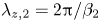 $\lambda _{z,2}=2{\rm \pi} /\beta _2$. At the first three locations, mode (0, 1) dominates the disturbance, and its amplitude still follows the linear growth. Co-rotating clockwise vortices are formed as viewed facing downstream, leading to the upwash and downwash of fluids. Further downstream, the rapid growth of other modes results in the classic co-rotating rollover (or half-mushroom-like) structures in the cross-flow vortices. However, the rollover structures are somewhat degenerated at the last two locations because of the modes’ decay. Compared with the laminar flow, the stationary cross-flow vortices strongly promote the exchange of momentum, mass and energy between the fluids at different $\eta$.
6.2. Preparatory analysis
The development of the stationary cross-flow vortex itself does not directly lead to turbulence. Instead, high- and low-frequency waves induced by the cross-flow vortex play important roles. Here the secondary instability of stationary cross-flow vortex is analysed using SIT, based on the distorted mean flow in figure 17. Previous studies suggested that the characteristics of secondary cross-flow instability modes were tightly related to the distribution of mean-flow gradients (Malik et al. Reference Malik, Li, Choudhari and Chang1999). Thereby, the gradient contours of streamwise momentum  $\bar {\rho }^\prime \bar {u}_2^\prime$ in the wall-normal ( $\eta _2$) and spanwise ( $z_2$) directions are depicted in figure 18 at different $s$. At $s=0.5\,\textrm {m}$, the wall-normal shear mainly concentrates near the wall, and its magnitude is much larger than the spanwise shear. Further downstream, the spanwise shear rapidly increases with the growth of harmonic waves. Its two positive extrema are located at the downwash and the inner side of the upwash regions, while the negative extremum lies at the outer side of the upwash region. For the wall-normal shear, an additional peak appears on top of the vortex at $s=0.8\,\textrm {m}$. However, this peak is weakened further downstream due to the increase of vortex thickness, as shown in figure 18(c).
Contours of the gradients of streamwise ( $s_2$) momentum in the (a–c) wall-normal and (d–f) spanwise directions. Three streamwise locations are $s$ of (a,d) 0.5 m, (b,e) 0.8 m and (c, f) 1.1 m. The white dotted lines are the contours of the base streamwise velocity as in figure 17(b).

Next, a convergence study is conducted to determine the required  $N_{sd}$ (see (3.13)) for SIT. Also, an examination is required on whether $N_{max}=32$ is adequate to ensure an accurate base flow. The details of these two parts are provided in the supplementary material. The conclusion is that $N_{sd}=18$ and $N_{max}=32$ are adequate and adopted for later calculations; $\sigma _d$ is set to 0 and no distinctions are made between the fundamental, subharmonic and detuned modes.
6.3. Energy budget analysis
The classification of unstable secondary instability modes into type I ( $z$), type II ( $y$) or other types is based on their production mechanisms through the energy budget analysis (Malik et al. Reference Malik, Li, Choudhari and Chang1999), so a definition of the disturbance energy is required first. In incompressible flows, the disturbance energy is usually measured by the disturbance kinetic energy:
 \begin{equation} 2 \tilde{E}_{k} = \bar{\rho} {\left| \tilde{\boldsymbol u} \right|^2} = \tilde{\boldsymbol q}^{\mathrm{H}} {{\boldsymbol{\mathsf{M}}}}_k \tilde{\boldsymbol q}, \end{equation}
where  $\tilde {\boldsymbol q}$ is defined in § 3.2, the superscript $\mathrm {H}$ represents a conjugate transpose and ${{\boldsymbol{\mathsf{M}}}}_k$ is the energy-norm matrix. For hypersonic flows, however, the density and temperature disturbances can have large amplitudes (see figure 15), but they are not reflected in (6.1). Therefore, a question is raised as to how to define an appropriate energy norm for hypersonic and TCNE flows. To take into account the contribution from each component of $\tilde {\boldsymbol q}$, following the physically based derivation by Chu (Reference Chu1965), we use the following form of energy norm for TCNE flows (see Franko Reference Franko2011; Chen, Wang & Fu Reference Chen, Wang and Fu2022):
 $$\begin{align} 2 \tilde{E}_q &=
\bar{\rho} {\left| \tilde{\boldsymbol u} \right|^2} +
\frac{\bar{T} R}{\bar{\rho}} \left|\tilde{\rho}\right|^2 +
\bar{\rho} \bar{T} \sum_{s,m} {R_{Y,sm} \tilde{Y}_s^{\dagger}
\tilde{Y}_m} + \bar{T} \sum _m R_m
\left(\tilde{\rho}^{\dagger} \tilde{Y}_m + \tilde{\rho}
\tilde{Y}_m^{\dagger}\right) \nonumber\\ &\quad + \frac{\bar{\rho}
\bar{c}_{v,t-r}}{\bar{T}} \left|\tilde{T}\right|^2 +
\frac{\bar{\rho} \bar{c}_{vib}}{\bar{T}}
\left|\tilde{T}_v\right|^2 = \tilde{\boldsymbol
q}^{\mathrm{H}} {{\boldsymbol{\mathsf{M}}}}_q \tilde{\boldsymbol q} ,
\end{align}$$
$$\begin{align} 2 \tilde{E}_q &=
\bar{\rho} {\left| \tilde{\boldsymbol u} \right|^2} +
\frac{\bar{T} R}{\bar{\rho}} \left|\tilde{\rho}\right|^2 +
\bar{\rho} \bar{T} \sum_{s,m} {R_{Y,sm} \tilde{Y}_s^{\dagger}
\tilde{Y}_m} + \bar{T} \sum _m R_m
\left(\tilde{\rho}^{\dagger} \tilde{Y}_m + \tilde{\rho}
\tilde{Y}_m^{\dagger}\right) \nonumber\\ &\quad + \frac{\bar{\rho}
\bar{c}_{v,t-r}}{\bar{T}} \left|\tilde{T}\right|^2 +
\frac{\bar{\rho} \bar{c}_{vib}}{\bar{T}}
\left|\tilde{T}_v\right|^2 = \tilde{\boldsymbol
q}^{\mathrm{H}} {{\boldsymbol{\mathsf{M}}}}_q \tilde{\boldsymbol q} ,
\end{align}$$
where  ${\dagger}$ denotes the complex conjugate and ${R_{Y,sm}}$ is a species-related coefficient matrix. For CPG flows, (6.2) reduces to the same form as that widely used in the transient growth analysis (Hanifi, Schmid & Henningson Reference Hanifi, Schmid and Henningson1996). The subscripts ‘ $k$’ and ‘ $q$’ are used below to distinguish the energy-related terms based on $\tilde {E}_{k}$ and $\tilde {E}_{q}$, respectively.
The governing equation of the disturbance energy norm is obtained after left-multiplying  $\tilde {\boldsymbol q}^{\mathrm {H}} {{\boldsymbol{\mathsf{M}}}} {{\boldsymbol{\mathsf{F}}}}^{-1}$ to (3.2), where ${{\boldsymbol{\mathsf{M}}}}$ is either ${{\boldsymbol{\mathsf{M}}}}_k$ or ${{\boldsymbol{\mathsf{M}}}}_q$. For SIT, the base flow and the disturbance are replaced with $\bar {\boldsymbol q}_2^\prime$ and $\tilde {\boldsymbol q}_{2,{ sd}}$, respectively (see § 3.3). The resulting classified energy-norm equation in SIT is written as
 \begin{equation} \frac{\mathrm{D} \tilde{E}_{sd}}{\mathrm{D} t} = \mathcal{P}_y + \mathcal{P}_z + \varXi + \varPi + \mathcal{V} + \mathcal{S}, \end{equation}
where  $\tilde {E}_{sd}$ is the energy norm of $\tilde {\boldsymbol q}_{2,{ sd}}$. Terms $\mathcal {P}_y$ and $\mathcal {P}_z$ are the production terms due to the wall-normal and spanwise gradients, respectively. Term $\varXi$ is the production term due to the streamwise gradients and is negligible under the parallel-flow assumption. Term $\varPi$ represents the diffusion and dilatation work contributions by the pressure disturbance. Term $\mathcal {V}$ denotes the viscous diffusion and dissipation terms related to $\mu$, $\kappa _{t-r}$, $\kappa _{v}$ and $D_{sm}$. Term $\mathcal {S}$ is the energy transfer term due to the disturbance of TCNE source terms. Detailed expressions of these terms can be found in Chen et al. (Reference Chen, Wang and Fu2022). If $\tilde {E}_{sd}$ takes the form of $\tilde {E}_{{ sd},k}$ in (6.1), the production terms are expressed as
 \begin{equation} \mathcal{P}_{y,k} ={-}\mathrm{Re} \left( \bar{\rho}^\prime \tilde{u}_{2,{ sd}}^{\dagger} \tilde{v}_{2,{ sd}} \frac{\partial \bar{U}_2^\prime}{\partial \eta_2} \right), \quad \mathcal{P}_{z,k} ={-}\mathrm{Re} \left( \bar{\rho}^\prime \tilde{u}_{2,{ sd}}^{\dagger} \tilde{w}_{2,{ sd}} \frac{\partial \bar{U}_2^\prime}{\partial z_2} \right), \end{equation}
where  $\mathrm {Re}({\cdot })$ denotes the real part of complex variables. If $\tilde {E}_{sd}$ is $\tilde {E}_{{ sd},q}$ in (6.2), then $\mathcal {P}_{y,q}$ and $\mathcal {P}_{z,q}$ contain extra terms related to the gradients of $\bar {\rho }^\prime$, $\bar {T}^\prime$, $\bar {T}_v^\prime$ and $\bar {Y}_s^\prime$. After a spatial integration in the $\eta _2$– $z_2$ plane, the growth rate of a secondary instability mode is decomposed as (Malik et al. Reference Malik, Li, Choudhari and Chang1999; Xu et al. Reference Xu, Chen, Liu, Dong and Fu2019)
 \begin{equation} \omega_{s,r} = \sigma_{P_y} + \sigma_{P_z} + \sigma_{\varXi} + \sigma_{\varPi} + \sigma_{V} + \sigma_{S}, \end{equation}
where  $\sigma _{\phi }$ is the growth-rate contribution from the term $\phi$ ( $\mathcal {P}$, $\mathcal {V}$ or others):
 \begin{equation} \sigma_{\phi} = \frac{2}{E_I} \int_{0}^{2{\rm \pi}/\beta_2} { \int_{0}^{\infty} {\phi\,\mathrm{d} \eta_2}\,\mathrm{d}z_2 }, \quad E_I = \int_{0}^{2{\rm \pi}/\beta_2} { \int_{0}^{\infty} {\tilde{E}_{sd}\,\mathrm{d} \eta_2}\,\mathrm{d}z_2}. \end{equation}
Consequently, the contribution from each term on the right-hand side of (6.3) to the disturbance growth rate is quantified.
We now compare the results based on the two energy norms in (6.1) and (6.2). Figure 19 provides the decomposed growth rate with different frequencies for three representative secondary instability modes at  $s=1.0\,\textrm {m}$. The shapes of these modes are further discussed in § 6.4. For all the modes here, $\mathcal {P}_y$, $\mathcal {P}_z$ and $\mathcal {V}$ are the main three contributing terms, while the other three terms are insignificant to the growth rate. One can see that $\mathcal {V}$ always has a negative contribution to the mode's growth, and this stabilizing effect tends to be stronger with a frequency increase. In comparison, the two production terms support the growth of modes, but they also have negative contributions within some frequency ranges. In general, the decomposed growth rates based on the two energy norms differ only slightly, though the differences slowly increase with frequency. In fact, though $|\tilde {T}_{sd}|$ is an order of magnitude larger than $|\tilde {u}_{2, sd}|$ for the modes in figure 19, the term ${\bar {\rho }^\prime \bar {c}_{v,t-r}^\prime }/{\bar {T}^\prime } |\tilde {T}_{sd}|^2/2$ (denoted as ET) in (6.2) is smaller than $\bar {\rho }^\prime {|\tilde {\boldsymbol u}_{2,{ sd}}|^2}/2$ (termed as EU), as shown in figure 19(d). Term EU makes up roughly 50 %–80 % of $\tilde {E}_{sd}$ after a spanwise average for all the unstable secondary instability modes here. Thereby, it is concluded that the energy-norm choice between (6.1) and (6.2) does not change the classification of secondary instability modes based on the energy budget analysis. The energy norm in (6.2) is employed for later use. For the modes in figure 19(a,b), $\sigma _{P_z}$ is dominant while $\sigma _{P_y}$ is negative, so these two modes are classified as type-I modes. However, a difficulty is encountered for the mode in figure 19(c) in that neither $\sigma _{P_y}$ nor $\sigma _{P_z}$ shows a clear dominance on the mode's growth. It seems that the mode classification is not unique based on the production terms, but physically there is no mode switch. The mode that received comparable contribution from $\sigma _{P_y}$ and $\sigma _{P_z}$ was termed as a $y$/
$y$/ $z$ mode by Li et al. (Reference Li, Choudhari, Duan and Chang2014). More discussions on the mode classification are provided in § 6.4.
Contribution from different terms in (6.5) to the disturbance growth rates for (a) type-I-1, (b) type-I-2 and (c) type-IV-1 modes at  $s=1.0\,\textrm {m}$ based on the two energy norms in (6.1) (subscript ‘ $k$’) and (6.2) (subscript ‘ $q$’). The mode names used are discussed in § 6.4. (d) Profiles of the spanwise-averaged components of $\tilde {E}_{{ sd},q}$ normalized by the maximum energy norm (type-IV-1 mode at $f=197\,\textrm {kHz}$).

6.4. Characteristics of various modes
For an overview of the results at  $s=1.0\,\textrm {m}$ in the TCNE benchmark case, the growth rates, phase velocities and spatial distributions of the unstable secondary instability modes are plotted in figure 20. There are minor differences among the contours of $|\tilde {u}_{2,{ sd}}|$, $|\tilde {T}_{{ sd}}|$ and $\tilde {E}_{sd}$ normalized by their maximums. Hence the contours of $|\tilde {u}_{2,{ sd}}|/\max |\tilde {u}_{2,{ sd}}|$ are used to exhibit the modes’ spatial distribution.
(a) Growth rates and (b) phase velocities of secondary instability modes at  $s=1.0\,\textrm {m}$ in the TCNE benchmark case, as well as (c) contours of their normalized streamwise ( $s_2$) velocity amplitudes of the most unstable one. The white dotted lines are the contours of the base streamwise velocity as in figure 17(b).

Same as those in lower-speed flows, the frequency ranges of secondary instability modes are an order of magnitude larger than that of the primary instability (see figure 8), and the maximum frequency is as high as 425 kHz. These unstable modes are classified into the type-I or type-II modes as discussed in § 6.3. In addition, a new series of type-IV modes are defined here, which receive combined contribution from  $\mathcal {P}_y$ and $\mathcal {P}_z$, and have unique distributions rarely reported before, as is discussed at length later. Correspondingly, the three modes in figure 19 are named type-I-1, type-I-2 and type-IV-1 modes, respectively. As can be seen, the low-frequency type-I-1 mode has the highest maximum growth rate and the lowest phase velocity at $s=1.0\,\textrm {m}$. Its frequency at the largest growth rate is 65 kHz, which is only a half or a third of those of other modes. Besides, the type-I-1 mode locates at the outer side of the upwash region of the vortex, where the spanwise shear is the negative extremum (see figure 18). This is consistent with the classic distribution of type-I modes observed in lower-speed flows (White & Saric Reference White and Saric2005; Craig & Saric Reference Craig and Saric2016). In comparison, the type-I-2 mode locates at an upper region with a much lower growth rate. The spatial distribution of this mode looks similar to that of the traditional type-II mode, but the energy budget analysis in figure 19(b) demonstrates its classification as a type-I mode. The type-II1 mode is found on top of the vortex, where the wall-normal shear is much stronger than the spanwise shear. This is also a classic location for type-II modes (Malik et al. Reference Malik, Li, Choudhari and Chang1999). The two type-II-2 modes displayed have wide unstable frequency ranges and high phase velocities. Moreover, they are located near the trough of the vortex, similar to the location of the modes reported by Koch et al. (Reference Koch, Bertolotti, Stolte and Hein2000) as a type-III mode, and by Xu et al. (Reference Xu, Chen, Liu, Dong and Fu2019) as a new $y$ mode.
In addition, another class of modes, termed type-IV modes, are found at higher frequencies. The three type-IV modes shown all have relatively large growth rates and are located at the downwash region of the vortex. In the following, the energy budget analysis is employed to study the contribution from  $\mathcal {P}_y$ and $\mathcal {P}_z$ to the type-IV-2 mode, dominating the linear growth regime of the secondary instability (shown in figure 24 later). Figure 21 gives the growth rate decomposition and the spatial distributions of $\tilde {E}_{sd}$, $\mathcal {P}_{y}$ and $\mathcal {P}_{z}$ (normalized by $\max _{y,z} \tilde {E}_q$ and $\omega _{s,r}$) at a sequence of streamwise locations. One important observation is that $\sigma _{P_y}$ and $\sigma _{P_z}$ alternately dominate the mode growth at different $s$. Specifically, $\sigma _{P_y}$ is dominant upstream of 0.75 m, and $\mathcal {P}_{y}$ mainly concentrates on top of the vortex. Further downstream, $\sigma _{P_y}$ decreases and $\sigma _{P_z}$ grows to be dominant. Term $\mathcal {P}_{z}$ is mainly located at the downwash region of the vortex, in connection with local high spanwise shear as shown in figure 18(e, f). The hot zone of $\mathcal {P}_{z}$ gradually rotates clockwise as viewed facing upstream and moves to the right-hand side of the vortex at $s>0.90\,\textrm {m}$. Meanwhile, $\sigma _{P_z}$ also drops further downstream, leading to the rapid decrease of $\omega _{s,r}$. Meanwhile, $\sigma _{P_y}$ slowly increases and surpasses $\sigma _{P_z}$ at $s=1.10\,\textrm {m}$, which is mainly contributed by the production term near the trough of the vortex. In short, the type-IV-2 mode is located primarily in the downwash region of the cross-flow vortex (contributed by $\sigma _{P_z}$), and also has distributions on top or trough of the vortex (contributed by $\sigma _{P_y}$) at different streamwise locations, which is essentially different from the type-I or type-II modes. Many more unstable modes are also found in figure 20, but are not discussed in detail here because of their relatively low growth rates.
Streamwise development of the type-IV-2 mode at  $s$ of (a) 0.70 m, (b) 0.80 m, (c) 0.90 m, (d) 1.00 m and (e) 1.10 m. (i) The growth rate decomposition, and (ii)–(iv) the contours of the normalized disturbance energy, wall-normal and spanwise production terms, respectively.

The streamwise evolutions of the secondary instability modes in figure 20 are further investigated to provide a comprehensive knowledge of their characteristics for this flow. Moyes et al. (Reference Moyes, Kocian, Mullen and Reed2018) pointed out the correlation between the transition onset and the neutral point of secondary cross-flow instability in the HIFiRE-5b flow case. Downstream of the neutral point, various unstable modes appear, and their growth rates and shapes are plotted in figure 22 at  $s=0.65\,\textrm {m}$, 0.75 m, 0.90 m and 1.10 m. Here $s=0.75\,\textrm {m}$ is near the location where all Fourier modes in NPSE reach their largest amplitudes (see figure 17a). The evolution of four representative modes, namely type-II1, type-IV-1, type-I-1 and type-IV-2 modes, is tracked, while the growth rates of other modes are also plotted. The type-II1 mode rides on top of the vortex, and reaches its highest growth rate at $s=0.81\,\textrm {m}$. Further downstream, its growth rate decreases, and the mode is stable downstream of $s=1.10\,\textrm {m}$. This stabilization is accompanied by the weakening of the wall-normal shear, as reflected in figure 18. The streamwise evolution of the type-IV-2 mode has been discussed in relation to figure 21. It is the most unstable one at $s=0.65\,\textrm {m}$ and 0.75 m, but further downstream its growth rate also quickly decreases and the frequency shifts to a lower range. The type-IV-1 mode has a similar distribution pattern to the type-IV-2 mode. Its growth rate surpasses that of the type-IV-2 mode at $s=0.90\,\textrm {m}$ and then drops. In comparison, the type-I-1 mode is destabilized to be the most unstable mode downstream at $s=1.0\,\textrm {m}$ owing to local strong spanwise shear. Its frequency is below 200 kHz, and it is located at the outer side of the upwash region of the vortex. Furthermore, the orientation of its concentration area is nearly perpendicular to the wall at $s=1.1\,\textrm {m}$ owing to the increase of the vortex thickness.
Streamwise development of the secondary instability modes at  $s$ of (a) 0.65 m, (b) 0.75 m, (c) 0.90 m and (d) 1.10 m. (i) The growth rate, and the normalized streamwise velocity amplitudes of (ii) type-II1, (iii) type-IV-1 and (iv) type-I-1 modes. The colourbar is the same as that in figure 20.

It is worth mentioning that Groot et al. (Reference Groot, Serpieri, Pinna and Kotsonis2018) (their figure 8) found two unstable modes of secondary cross-flow instability that had similar distribution to the type-IV modes in the present case (specifically, figures 21b(ii) and 22a(iii)) in their biglobal analyses on an incompressible flow. These modes were not analysed in detail in their study because they did not have the largest growth rate. Nevertheless, their results support the findings of the present paper. In fact, as is shown in § 6.5, the growth rates of the type-IV modes are not the largest in the CPG case, but they are largely destabilized in the TCNE cases.
The phase information of modes is missing in figure 22. Hence (3.13) is used to reproduce the three-dimensional ( $s_2$– $\eta _2$– $z_2$) distribution of $\tilde {u}_{2, sd}$, which is applicable under the locally-parallel-flow assumption. Figure 23 illustrates the spatial structures of $\tilde {u}_{2, sd}$ of the four modes near $s=0.90\,\textrm {m}$. The temporal sequence ( $t$–
$t$– $\eta _2$– $z_2$) of $\tilde {u}_{2, sd}$ at a fixed $s_2$ exhibits the same structures except in the opposite ( $-t$) direction. Alternating inclined strips are observed for $\tilde {u}_{2, sd}$ of the type-I mode, which is quite similar to those documented in the low-speed experiments through a proper orthogonal decomposition (Groot et al. Reference Groot, Serpieri, Pinna and Kotsonis2018). Also, the streamwise wavelength ( $2{\rm \pi} /\alpha _s$) of the type-I mode is several times larger than that of the other three modes. For the type-II1 mode, inclined curved strips are observed on the top of the vortex. Their orientation is consistent with the base-flow streamlines. In comparison, the two type-IV modes exhibit aligned-arrow and inclined-dumbbell shapes in the downwash region of the vortex.
Isosurfaces of the normalized streamwise velocity ( $\mathrm {Re}(\tilde {u}_{2, sd})/\max |\tilde {u}_{2, sd}|=\pm 0.2$) for the modes near $s=0.9\,\textrm {m}$: (a) type-I-1, (b) type-II1, (c) type-IV-1 and (d) type-IV-2 modes. The black solid lines are the contours of the base streamwise velocity and the red dash-dotted lines the contours of $|\tilde {u}_{2, sd}|/\max |\tilde {u}_{2, sd}|$ at 0.2.

Next, we focus on the accumulative growth ( $N$ factors) of these secondary instability modes in the streamwise direction to find the spatially dominant one. There are generally two approaches to obtain the spatial growth rate. The first is to solve the spatial-mode version of (3.13), i.e. solve for the complex $\alpha _s$ at a given real $\omega _s$. The second is to use the extended Gaster transformation (see Koch et al. Reference Koch, Bertolotti, Stolte and Hein2000), where the temporal growth rate is transformed to a spatial one through a group velocity. Comparisons show that the growth rate differences of the type-I-1, type-II1 and type-IV modes by these two methods are less than 2 % at $s=1.0\,\textrm {m}$, so the extended Gaster transformation also works in this high-enthalpy flow. Nevertheless, small differences exist so the spatial-mode calculation is performed in the following to obtain the disturbance $N$ factors. Figure 24 gives the $N$ factor distribution of the four modes in figure 22 at the frequencies related to their maximum growth rates. The $N$ factor envelopes within specific frequency bands are also plotted. The type-IV-2 mode is observed to have the largest $N$ factor with the onset at $s=0.59\,\textrm {m}$. The $N$ factors of the type-IV-1 and type-II1 modes are close to each other, and the $N$ factor of the type-I-1 mode is the lowest within the computational domain. In short, the present results highlight the vital role of the type-IV modes. This is the first report, to the authors’ knowledge, wherein a secondary instability mode, located at the downwash region of the stationary cross-flow vortex, has the largest $N$ factor in hypersonic boundary layers.
Streamwise distribution of the  $N$ factors for the four secondary instability modes in the TCNE benchmark case (a) at the frequencies related to their local maximum growth rates and (b) within specific frequency bands with $\Delta f=10\,\textrm {kHz}$.

It is important to note that the type-IV-2 mode might not necessarily dominate the secondary instability region, because the initial amplitudes of different modes can significantly differ under specific conditions. Similar phenomena exist in some lower-speed flows in that the type-II mode was not observed in experiments or DNS results though its growth rate was comparable with that of the type-I mode from SIT (Bonfigli & Kloker Reference Bonfigli and Kloker2007; Craig & Saric Reference Craig and Saric2016; Chen et al. Reference Chen, Dong, Chen, Yuan and Xu2021a). This might be attributed to the higher receptivity coefficient of the type-I mode in those cases. Therefore, a receptivity analysis is required in the future, in combination with SIT, to determine the initial amplitudes and subsequent growth of different modes.
Finally, as the type-IV modes were rarely reported before, a parameter study of wall temperatures and gas models is performed to examine their effects. Note that for flows with different parameters, the difference in the primary instability makes it hard to isolate the effects of the parameters on the secondary instability. Therefore, we make a direct comparison between the secondary instability results of the most unstable stationary cross-flow vortex with the same initial amplitude of the primary disturbance. This is designed to study the most likely change under the same free-stream perturbation conditions. Therefore, the change in secondary instability characteristics results from the combined effects of the differences in the laminar flow, vortex saturation amplitude, the streamwise location of the saturation region (thus local Reynolds number and boundary layer thickness), and so on.
6.5. Effects of wall temperature and TCNE
As a parameter study, the nonlinear evolution and secondary instability of the stationary cross-flow vortices in the adia-TCNE and adia-CPG cases are also calculated. In the NPSE calculation, the spanwise wavelengths of mode (0, 1) in the two cases are both selected to be 40 mm with the neutral point (also the computational onset) at  $s=0.04\,\textrm {m}$, based on the results in figure 12. The initial amplitudes of mode (0, 1) are set to 0.1 % as well. The streamwise development of the mode amplitudes is plotted in figure 25. As can be seen, the amplitude evolution in the two adiabatic-wall cases bears a strong resemblance to that in figure 17(a) except for the higher growth rates upstream of the saturation region due to $T_w$ increase. Mode (0, 1) begins to saturate at $s=0.39\,\textrm {m}$ and 0.47 m in the adia-TCNE and adia-CPG cases, respectively.
Streamwise development of the mode amplitudes in (a) adia-TCNE and (b) adia-CPG cases.

The contours of  $\bar {T}^\prime$ in the adia-CPG case are depicted in figure 26(a) at $s=0.45\,\textrm {m}$ and 0.60 m. These two locations are upstream and downstream where all Fourier modes reach their maximum amplitudes, respectively. In the same way, the contours of $\bar {T}^\prime$, $\bar {T}_v^\prime$ and $\bar {Y}_{O_2}^\prime$ in the adia-TCNE case are provided in figure 26(b–d) at $s=0.40\,\textrm {m}$ and 0.55 m. The laminar counterpart is also provided for comparison. The local velocity vectors $[\bar {w}_2^\prime,\bar {v}_2^\prime ]$ are displayed to help identify the fluid motion due to cross-flow vortex. From the $\bar {T}^\prime$ contours, high-temperature regions are observed in the two cases near the wall between the stems of two adjacent vortices. The maximum temperature in the adia-TCNE case is 16.5 % higher than the laminar $T_w$ at $s=0.55\,\textrm {m}$, while in the adia-CPG case the difference is less than 1 %. This is because the mixing of fluids leads to the energy absorbed by the energy relaxation and chemical reactions being released again. In addition, the temperature near the stem of the rollover structure is reduced in the adia-TCNE case, but in the adia-CPG case the stem is a high-temperature region. This difference is explained from the contours of $\bar {T}_v^\prime$ and $\bar {Y}_{O}^\prime$, whose maximums are at the stem of the rollover. This is associated with the local low speed and thus low Damköhler number, so the flow is closer to thermochemical equilibrium and the temperature is reduced. The rollover structures are clearly recognized from the contours of $\bar {T}_v^\prime$ and $\bar {Y}_{O}^\prime$. This indicates the overall and thus more structurally analogous influence of the cross-flow vortices on essential variables.
(a) Contours of the temperature at  $s$ of (i) 0.45 m and (ii) 0.60 m in the adia-CPG case. Contours of (b) temperature, (c) vibrational temperature and (d) mass fraction at $s$ of (i) 0.40 m and (ii) 0.55 m in the adia-TCNE case.

Next, the secondary cross-flow instability in the adia-TCNE case is calculated. The growth rates and shape functions of the unstable modes from SIT are plotted in figure 27 at  $s=0.45\,\textrm {m}$. As can be seen, the most unstable four modes are the same as those in the TCNE benchmark case: type-I-1, type-II1, type-IV-1 and type-IV-2 modes. The two type-IV modes have the largest growth rate and they are located at the downwash region of the cross-flow vortex. In addition, the type-IV-1 mode has a distribution at the trough of the vortex, which is contributed by $\mathcal {P}_{y}$ as discussed in § 6.4. Subsequently, the $N$ factor envelopes of the type-I-1, type-II1 and type-IV-2 modes are calculated within specific frequency bands, as shown in figure 28. Again, the type-IV mode has the largest $N$ factor in the computational domain, while the type-I-1 mode has the lowest. Therefore, the type-IV mode has the largest $N$ factors in both the benchmark TCNE and adia-TCNE cases.
(a) Growth rates of unstable secondary instability modes with different frequencies at  $s=0.45\,\textrm {m}$ in the adia-TCNE case. (b) Contours of their normalized streamwise velocities at the frequencies corresponding to the largest growth rates.

Streamwise distribution of the  $N$ factors for the three secondary instability modes in the adia-TCNE case within specific frequency bands with $\Delta f=10\,\textrm {kHz}$.

A further quantitative comparison indicates two moderate influences due to  $T_w$ increase. The first is that both the type-II1 and type-IV modes are somewhat stabilized in comparison with that in figure 24. The second is the frequency increase of the type-I-1 mode relative to the type-II1 and type-IV modes. These two influences can both be associated with the change of the boundary layer thickness. Specifically, previous investigations suggested that with an increase of ${\textit {Re}}_\infty$, a thinner boundary layer leads to the destabilization and frequency increase of the type-II mode. The former effect was through the strengthening of the wall-normal shear (see Malik et al. Reference Malik, Li, Choudhari and Chang1999; White & Saric Reference White and Saric2005). In the present case, the increase of $T_w$ leads to a thicker boundary layer, but the secondary instability region moves upstream due to the stronger primary instability, decreasing the local boundary layer thickness. As the outcome of these two competing effects, the type-II1 and also the type-IV modes are slightly stabilized, and the frequency of the type-I-1 mode rises.
For the adia-CPG case, the secondary instability modes of the stationary cross-flow vortices in figure 25(b) are also analysed to examine the effect of TCNE. Figure 29 provides the growth rates of the unstable modes at  $s=0.50\,\textrm {m}$ and 0.60 m. The growth rate results are found to be significantly different from the TCNE benchmark and adia-TCNE cases, indicating the essential influence of TCNE on the secondary cross-flow instability. We also notice that the results in figure 29(a) are quite similar to figure 12 in Xu et al. (Reference Xu, Chen, Liu, Dong and Fu2019) for a Mach-6 swept-parabola case with an adiabatic-wall condition. Both identify a dominant type-I mode, a low-frequency type-III mode (following that in the reference) and low-growth-rate type-II modes. Also, the frequency of the type-I mode is comparable to that of the type-II modes, which reflects the insensitivity of cross-flow instability to free-stream Mach number. In addition, the type-IV mode is observed in the present CPG case, which is located at the downwash region and trough of the vortex. The frequency relation between the type-IV mode and the others also indicates that the type-IV mode is not the harmonic of either type-I or type-II modes, as noted by Groot et al. (Reference Groot, Serpieri, Pinna and Kotsonis2018). Further downstream to $s=0.60\,\textrm {m}$, the growth rates of the type-I and type-III modes decrease, while the those of the type-II1 and type-IV modes increase. The distribution of the type-I modes moves towards the top of the vortex, which also reflects the strengthening of the wall-normal shear.
Growth rates of the secondary instability modes with different frequencies at (a) 0.50 m and (b) 0.60 m in the adia-CPG case.

The comparison between the adia-CPG case and the two TCNE cases indicates that the type-IV modes are heavily destabilized by the TCNE effects, and the type-I modes are stabilized. Also, the frequency of the type-I mode is largely reduced by TCNE, relative to those of the type-II and type-IV modes. These changes are also consistent with the trends concerning the variation of the boundary layer thickness, as discussed above. The local thinner boundary layer in the TCNE cases is due to the temperature decrease and the destabilization of the primary instability (so the secondary instability region moves upstream). Furthermore, the destabilization of the type-IV modes is strongly related to the spanwise gradients of the base flow, as shown in figure 30. In the adia-CPG case, the two positive peaks of the spanwise shear are also located at the downwash region and the inner side of the upwash region, as discussed in relation to figure 18, but the peak amplitude in the downwash side is much lower than the other. In comparison, in the adia-TCNE case, the spanwise shear in the downwash region of the vortex is also of large amplitude. Therefore, the stronger downwash of fluids in the TCNE cases promotes the growth of the type-IV modes located in this region.
Contours of the spanwise gradients of streamwise momentum in (a–c) adia-CPG and (d–f) adia-TCNE cases. Three streamwise locations are (a,d) 0.45 m, (b,e) 0.55 m and (c, f) 0.60 m. The contour levels for all the panels are the same.

7. Conclusions
In this work, the cross-flow primary and secondary instabilities in hypersonic high-enthalpy boundary layers are analysed using LST, NPSE and SIT with TCNE effects. The flow over a swept parabola is calculated at  ${\textit {Ma}}_\infty$ of 16 under the TCNE and CPG models. The entropy layer induced by the strong bow shock leads to a high-temperature region and thus strong TCNE effects outside the boundary layer. Thereby, $T_e$ is reduced in the TCNE case, and ${\textit {Ma}}_e$ is generally 0.18–0.45 higher than that in the CPG case.
The results from LST identify unstable stationary and travelling cross-flow modes. The most unstable one is travelling, but its  $N$ factor at a fixed frequency is no higher than that of the stationary mode. The TCNE is shown to have a destabilizing effect on the cross-flow mode under the non-catalytic wall boundary condition, lifting the maximum $N$ factors by 1.8–3.0 within the computational domain as compared with the CPG case. With an adiabatic-wall condition, the difference of the maximum $N$ factors is narrowed, but the TCNE effect is still slightly destabilizing. To explain this effect, a parameter study is performed and two important non-dimensional parameters are summarized. One is the temperature ratio $T_w/T_e$ and the other is the cross-flow Mach number ${\textit {Ma}}_{cf}=|\bar {U}_{cf}|/a_f$. Increases of the two tend to destabilize the cross-flow mode, while the latter is more essential and works better for both TCNE and CPG cases. Therefore, the TCNE effects have three influences on the growth rate of the cross-flow mode. The first is to decrease the temperature and thus $a_f$ inside the boundary layer, which is destabilizing. The second is to decrease $T_e$, which is also destabilizing. The third is to decrease $T_w$ if $T_w$ is not fixed, which is stabilizing. The second effect is quite obvious for the cases with strong entropy layers and thus high $T_e$, such as the present parabola case. The third effect is most obvious under an adiabatic-wall condition. The simple relation (5.6) derived from the inviscid disturbance equations well predicts the disturbance shape functions except near the singularity point where $\bar {W}_2$ (the velocity perpendicular to the cross-flow vortex axis) is zero. This singularity point is also found very close to the GIP based on $\bar {W}_2$.
Using NPSE, the classic co-rotating rollover structures are observed in the saturated stationary cross-flow vortices. Compared with the laminar flow, the cross-flow vortices strongly promote the exchange of momentum, mass and energy between the fluids at different wall-normal heights. The SIT is employed to find the unstable secondary instability modes of cross-flow vortices. Two kinds of disturbance energy norms are used in the energy budget analysis to classify the modes. The first form only considers the disturbance kinetic energy, while the second form additionally takes into account the contribution from  $\hat {\rho }$, $\hat {T}$, $\hat {T}_v$ and $\hat {Y}_s$. Nevertheless, the difference of the growth-rate decomposition between the two is negligible. The traditional type-I ( $z$) and type-II ( $y$) modes are recognized. In the adia-CPG case, the type-I mode has the largest growth rate. However, the newly defined type-IV modes are observed to have the largest $N$ factors in the TCNE benchmark and adia-TCNE cases. Energy budget analysis indicates that the type-IV modes are located at the downwash region of the vortex and receive a combined contribution from the wall-normal (on top and trough of the vortex) and spanwise (in the downwash region) production terms. As compared with the CPG case, the destabilization of the type-IV modes in the TCNE cases is attributed to the stronger spanwise shear at the downwash region, as well as the thinner boundary layer due to the temperature decrease and the destabilized primary instability. Moreover, the type-IV modes are slightly stabilized with wall temperature increase.
Future efforts, including receptivity, DNS and experimental researches, are expected to further clarify the roles of different secondary instability modes downstream towards turbulence.
Supplementary material
Supplementary material is available at https://doi.org/10.1017/jfm.2022.607.
Acknowledgements
The authors are grateful for the insightful comments from the reviewers.
Funding
This work was supported by the National Key Research and Development Plan of China through project no. 2019YFA0405201 and the National Key Project (grant GJXM92579). The authors are also grateful for the support from NSFC grants 92052103 and 12172195. J.R. acknowledges the support of the Alexander von Humboldt foundation.
Declaration of interests
The authors report no conflict of interest.
Data availability statement
The data that support the findings of this study are available from the corresponding author upon reasonable request.


 Open access

