


1. Introduction
A classical branching Brownian motion (BBM) in $\mathbb{R}$
can be constructed as follows. Initially there is a single particle at the origin of the real line and this particle moves as a one-dimensional standard Brownian motion denoted by
$\mathbb{R}$
can be constructed as follows. Initially there is a single particle at the origin of the real line and this particle moves as a one-dimensional standard Brownian motion denoted by $B = \{B(t),\, t\geq 0 \}$
. After an independent exponential time with parameter 1, the initial particle dies and gives birth to L offspring, where L is a positive integer-valued random variable with distribution
$B = \{B(t),\, t\geq 0 \}$
. After an independent exponential time with parameter 1, the initial particle dies and gives birth to L offspring, where L is a positive integer-valued random variable with distribution $\{p_k\colon k\geq 1 \}$
. Here we assume that the expected number of offspring is two (i.e.
$\{p_k\colon k\geq 1 \}$
. Here we assume that the expected number of offspring is two (i.e. $\sum_{k=1}^{\infty} kp_k = 2$
) and the variance of the offspring distribution is finite (i.e.
$\sum_{k=1}^{\infty} kp_k = 2$
) and the variance of the offspring distribution is finite (i.e. $\sum_{k=1}^{\infty} k(k-1)p_k \lt \infty$
). Each offspring starts from its creation position and evolves independently, according to the same law as its parent. We denote the collection of particles alive at time t as
$\sum_{k=1}^{\infty} k(k-1)p_k \lt \infty$
). Each offspring starts from its creation position and evolves independently, according to the same law as its parent. We denote the collection of particles alive at time t as $N_t$
. For any
$N_t$
. For any $u\in N_t$
and
$u\in N_t$
and $s\le t$
, let
$s\le t$
, let $X_u(s)$
be the position at time s of particle u or its ancestor alive at that time.
$X_u(s)$
be the position at time s of particle u or its ancestor alive at that time.
In [Reference McKean19], McKean established a connection between BBM and the Fisher–Kolmogorov–Petrovskii–Piskounov (F-KPP) equation
 \begin{equation*} \frac{\partial u}{\partial t} = \frac{1}{2} \frac{\partial^2 u}{\partial x^2} + \sum_{k=1}^{\infty} p_k u^k - u.\end{equation*}
The F-KPP equation has received entensive attention using both analytic techniques [Reference Fisher8, Reference Kolmogorov, Petrovskii and Piskounov13] and probabilistic methods [Reference Bramson6, Reference Bramson7, Reference Harris11, Reference Kyprianou14, Reference McKean19].
Let’s recall some classical results on BBM and the F-KPP equation. Define $\mathbf{M}_t \,:\!=\, \max\{X_u(t)\colon u\in N_t \}$
. Bramson [Reference Bramson6] established that
$\mathbf{M}_t \,:\!=\, \max\{X_u(t)\colon u\in N_t \}$
. Bramson [Reference Bramson6] established that
 \begin{equation*} \lim_{t\to\infty}\mathbb{P}(\mathbf{M}_t - m_t \le z)=\lim_{t\to \infty} u(t,m_t+z)=w(z),\quad z\in \mathbb{R} ,\end{equation*}
where $m_t\,:\!=\, \sqrt{2} t-({3}/({2\sqrt{2}}))\log t$
and w solves the ordinary differential equation
$m_t\,:\!=\, \sqrt{2} t-({3}/({2\sqrt{2}}))\log t$
and w solves the ordinary differential equation $\frac{1}{2}w''+\sqrt{2}w'+\sum_{k=1}^{\infty} p_k w^k - w=0$
. Such a solution w is known as the traveling wave solution. Lalley and Sellke [Reference Lalley and Sellke15] provided the following representation of w for dyadic BBM:
$\frac{1}{2}w''+\sqrt{2}w'+\sum_{k=1}^{\infty} p_k w^k - w=0$
. Such a solution w is known as the traveling wave solution. Lalley and Sellke [Reference Lalley and Sellke15] provided the following representation of w for dyadic BBM:
 \begin{equation} w(z)\,:\!=\,\mathbb{E}\Big[\!\exp\!\Big\{{-}C_*{\mathrm{e}}^{-\sqrt{2}z}Z_{\infty}\Big\}\Big],\end{equation}
where $C_*$
is a positive constant and
$C_*$
is a positive constant and $Z_{\infty}$
is the limit of the derivative martingale of BBM. Specifically, define
$Z_{\infty}$
is the limit of the derivative martingale of BBM. Specifically, define
 \begin{equation*} Z_t = \sum_{u\in N_t} \big(\sqrt{2}t - X_u(t)\big){\mathrm{e}}^{\sqrt{2}(X_u(t)-\sqrt{2}t) };\end{equation*}
then $Z_t$
serves as the derivative martingale of the BBM. We denote by
$Z_t$
serves as the derivative martingale of the BBM. We denote by $Z_{\infty}$
the limit of
$Z_{\infty}$
the limit of $Z_t$
$Z_t$ $\mathbb{P}_x$
-almost surely (a.s.), as established in [Reference Kyprianou14, Reference Lalley and Sellke15]. It was also conjectured in [Reference Lalley and Sellke15] that the empirical (time-averaged) distribution of maximal displacement converges almost surely, that is,
$\mathbb{P}_x$
-almost surely (a.s.), as established in [Reference Kyprianou14, Reference Lalley and Sellke15]. It was also conjectured in [Reference Lalley and Sellke15] that the empirical (time-averaged) distribution of maximal displacement converges almost surely, that is,
 \begin{equation} \lim_{T\to\infty} \frac{1}{T} \int_0^T \mathbf{1}_{\{\mathbf{M}_s - m_s \leq x\}}\,\mathrm{d}s = \exp\!\big\{{-}C_* Z_{\infty}{\mathrm{e}}^{-\sqrt{2}x}\big\}, \quad \mbox{a.s.}\end{equation}
This conjecture was later confirmed in [Reference Arguin, Bovier and Kistler3].
In this paper, we consider the similar problem of BBM with absorption, where the particle is killed when it hits the absorbing barrier. The process can be defined as follows. Initially there is a single particle at $x>0$
and this particle evolves as the classical BBM with branching rate 1. We also assume that the number of offspring L has distribution
$x>0$
and this particle evolves as the classical BBM with branching rate 1. We also assume that the number of offspring L has distribution $\{p_k,\,k\geq 1\}$
with
$\{p_k,\,k\geq 1\}$
with $\mathbb{E} L = 2$
and
$\mathbb{E} L = 2$
and $\mathbb{E} L^2 \lt \infty$
. In addition, we add an absorbing barrier at the line
$\mathbb{E} L^2 \lt \infty$
. In addition, we add an absorbing barrier at the line $\{(y,t)\colon y= \rho t \}$
for some
$\{(y,t)\colon y= \rho t \}$
for some $\rho\in\mathbb{R}$
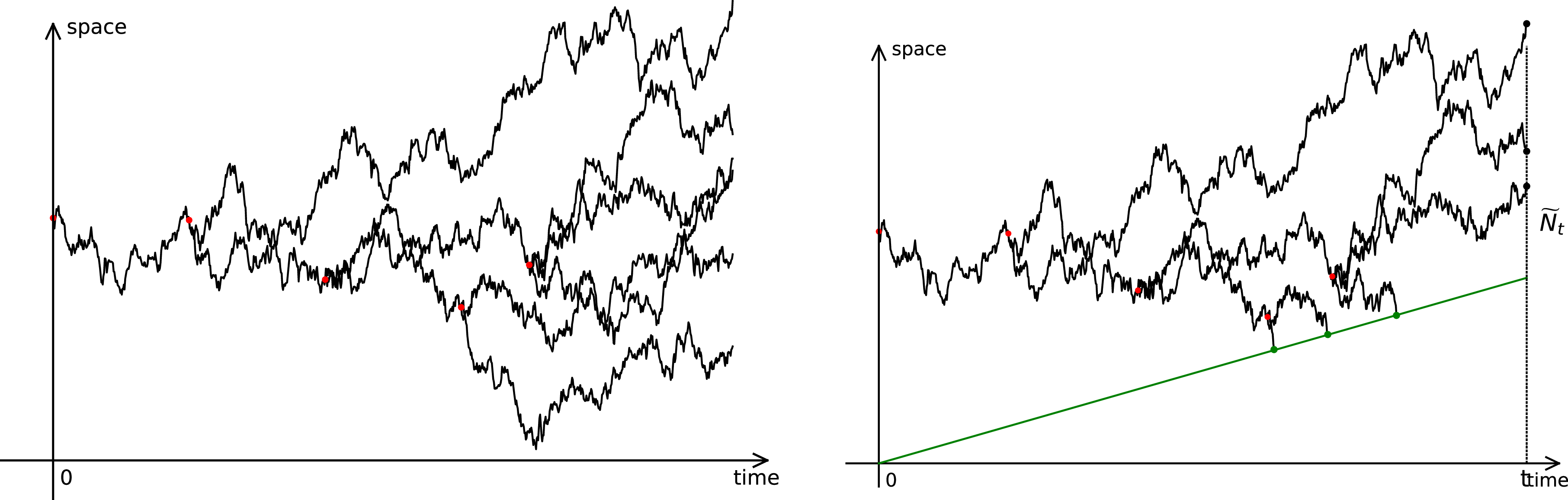
, i.e. particles hitting the barrier are instantly killed without producing offspring (see Figure 1).
$\rho\in\mathbb{R}$
, i.e. particles hitting the barrier are instantly killed without producing offspring (see Figure 1).
BBM and BBM with absorption.
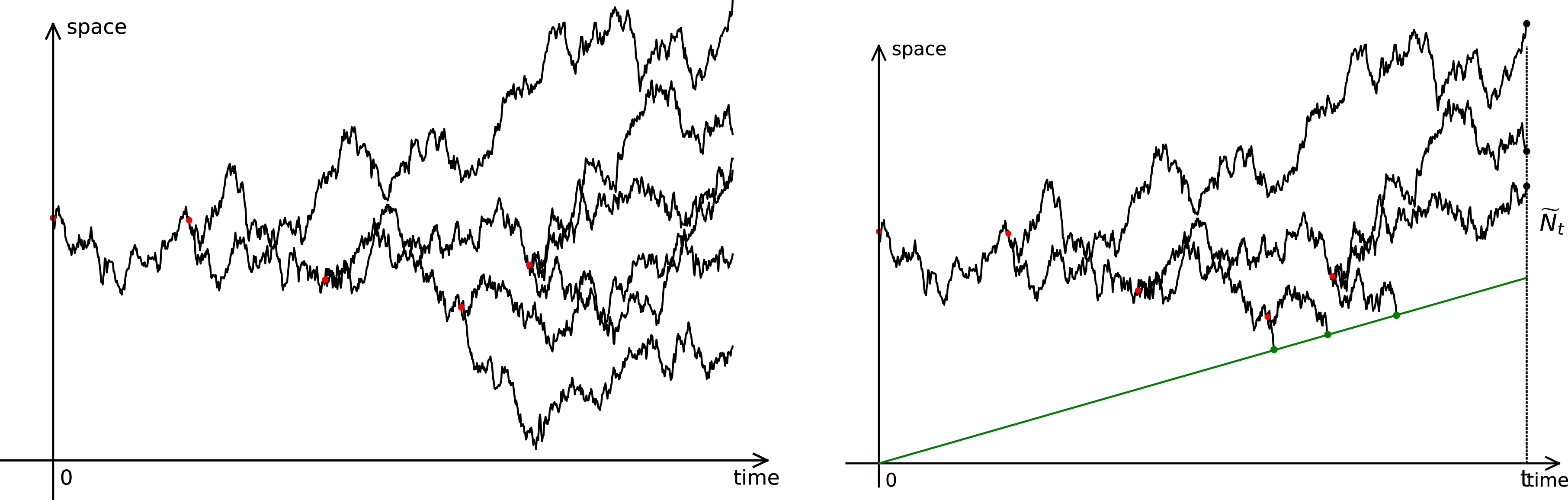
Figure 1 Long description
The image contains two line graphs side by side. Both graphs plot space on the y-axis against time on the x-axis. The left graph illustrates the branching and movement trajectories of particles in branching Brownian motion. The right graph includes an additional diagonal line emanating from zero and particles are absorbed upon hitting this line.
We use $\widetilde{N}_t$
to denote the set of the particles of the BBM with absorption that are still alive at time t. For any particle
$\widetilde{N}_t$
to denote the set of the particles of the BBM with absorption that are still alive at time t. For any particle $u\in \widetilde{N}_t$
and any time
$u\in \widetilde{N}_t$
and any time $s\leq t$
, we continue to use
$s\leq t$
, we continue to use $X_u(s)$
to represent the position of either particle u itself or its ancestor at time s. The extinction time of the BBM with absorption is defined as
$X_u(s)$
to represent the position of either particle u itself or its ancestor at time s. The extinction time of the BBM with absorption is defined as $\zeta\,:\!=\,\inf\{t>0\colon \widetilde{N}_t = \emptyset \}$
. Additionally, we define
$\zeta\,:\!=\,\inf\{t>0\colon \widetilde{N}_t = \emptyset \}$
. Additionally, we define $\widetilde{\mathbf{M}}_t$
as the maximum position among all particles
$\widetilde{\mathbf{M}}_t$
as the maximum position among all particles $u\in\widetilde{N}_t$
. The law of the BBM with absorption, starting from a single particle at position x, is denoted by
$u\in\widetilde{N}_t$
. The law of the BBM with absorption, starting from a single particle at position x, is denoted by $\mathbb{P}_x$
, and its expectation is denoted by
$\mathbb{P}_x$
, and its expectation is denoted by $\mathbb{E} _x$
.
$\mathbb{E} _x$
.
The asymptotic behavior of BBM with absorption has been extensively studied in the literature. Kesten [Reference Kesten12] demonstrated that the process dies out almost surely when $\rho \ge \sqrt{2}$
, while there is a positive probability of survival, i.e.
$\rho \ge \sqrt{2}$
, while there is a positive probability of survival, i.e. $\mathbb{P}_x(\zeta=\infty)>0$
, when
$\mathbb{P}_x(\zeta=\infty)>0$
, when $\rho \lt \sqrt{2}$
. Therefore,
$\rho \lt \sqrt{2}$
. Therefore, $\rho = \sqrt{2}$
is the critical drift separating the supercritical case
$\rho = \sqrt{2}$
is the critical drift separating the supercritical case $\rho \lt \sqrt{2}$
and the subcritical
$\rho \lt \sqrt{2}$
and the subcritical $\rho \gt \sqrt{2}$
. In the subcritical case, [Reference Harris and Harris9] provided the large-time asymptotic behavior for the survival probability. In the critical case, [Reference Kesten12] obtained upper and lower bounds on the survival probability, which were subsequently improved in [Reference Berestycki, Berestycki and Schweinsberg5, Reference Maillard and Schweinsberg18] further enhanced these results and investigated the behavior conditioned to survive. For BBM with absorption in the near-critical case, [Reference Berestycki, Berestycki and Schweinsberg4] and [Reference Liu16] are good references. In the supercritical case, [Reference Harris, Harris and Kyprianou10] studied properties of the right-most particle and the one-sided F-KPP traveling wave solution using probabilistic methods in the case of binary branching, specifically proving that
$\rho \gt \sqrt{2}$
. In the subcritical case, [Reference Harris and Harris9] provided the large-time asymptotic behavior for the survival probability. In the critical case, [Reference Kesten12] obtained upper and lower bounds on the survival probability, which were subsequently improved in [Reference Berestycki, Berestycki and Schweinsberg5, Reference Maillard and Schweinsberg18] further enhanced these results and investigated the behavior conditioned to survive. For BBM with absorption in the near-critical case, [Reference Berestycki, Berestycki and Schweinsberg4] and [Reference Liu16] are good references. In the supercritical case, [Reference Harris, Harris and Kyprianou10] studied properties of the right-most particle and the one-sided F-KPP traveling wave solution using probabilistic methods in the case of binary branching, specifically proving that $\lim_{t\to \infty} ({\widetilde{\mathbf{M}}_t}/{t})=\sqrt{2}$
on
$\lim_{t\to \infty} ({\widetilde{\mathbf{M}}_t}/{t})=\sqrt{2}$
on $\{\zeta=\infty\}$
,
$\{\zeta=\infty\}$
, $\mathbb{P}_x$
-a.s. and
$\mathbb{P}_x$
-a.s. and $g(x) \,:\!=\, \mathbb{P}_x(\zeta<\infty)$
is the unique solution to the one-side F-KPP traveling wave solution
$g(x) \,:\!=\, \mathbb{P}_x(\zeta<\infty)$
is the unique solution to the one-side F-KPP traveling wave solution
 \begin{equation*} \begin{cases} \dfrac{1}{2}g''-\rho g'+ g^2 -g = 0, \quad x>0, \\ g(0+)=1, g(\infty)=0. \end{cases} \end{equation*}
Louidor and Saglietti [Reference Louidor and Saglietti17] showed that the number of particles inside any fixed set, normalized by the mean population size, converges to an explicit limit almost surely. In this paper, we focus on the supercritical case, i.e. we always assume $\rho < \sqrt{2}$
.
$\rho < \sqrt{2}$
.
In [Reference Yang and Zhu20], we studied the maximal displacement and the extremal process of BBM with absorption. More precisely, we established the following result:
 \begin{equation*} \lim_{t\to \infty} \mathbb{P}_x(\widetilde{\mathbf{M}}_t - m_t\leq z) = \mathbb{E} _x\big(\!\exp\!\big\{{-}C_*\widetilde{Z}_{\infty}{\mathrm{e}}^{-\sqrt{2}z}\big\}\big),\end{equation*}
where $\widetilde{Z}_{\infty}$
is defined as the limit of
$\widetilde{Z}_{\infty}$
is defined as the limit of $\widetilde{Z}_t$
and
$\widetilde{Z}_t$
and $\widetilde{Z}_t \,:\!=\, \sum_{u\in \widetilde{N}_t} (\sqrt{2}t-X_u(t)){\mathrm{e}}^{\sqrt{2}(X_u(t)-\sqrt{2}t) }$
. It’s important to note that
$\widetilde{Z}_t \,:\!=\, \sum_{u\in \widetilde{N}_t} (\sqrt{2}t-X_u(t)){\mathrm{e}}^{\sqrt{2}(X_u(t)-\sqrt{2}t) }$
. It’s important to note that $\{\widetilde{Z}_t, t\geq 0, \mathbb{P}_x \}$
is not a martingale. However, according to [Reference Yang and Zhu20, Theorem 2.1], the limit
$\{\widetilde{Z}_t, t\geq 0, \mathbb{P}_x \}$
is not a martingale. However, according to [Reference Yang and Zhu20, Theorem 2.1], the limit $\widetilde{Z}_{\infty} \,:\!=\, \lim_{t\rightarrow\infty} \widetilde{Z}_t$
exists
$\widetilde{Z}_{\infty} \,:\!=\, \lim_{t\rightarrow\infty} \widetilde{Z}_t$
exists $\mathbb{P}_x$
-a.s. for any
$\mathbb{P}_x$
-a.s. for any $x>0$
and
$x>0$
and $\rho \lt \sqrt{2}$
. Similar to (1.2), our paper focuses on the empirical distribution function of the maximum of branching Brownian motion with absorption. We prove that the limit of this empirical distribution converges almost surely to a Gumbel distribution with a random shift. Here’s the statement of the main result.
$\rho \lt \sqrt{2}$
. Similar to (1.2), our paper focuses on the empirical distribution function of the maximum of branching Brownian motion with absorption. We prove that the limit of this empirical distribution converges almost surely to a Gumbel distribution with a random shift. Here’s the statement of the main result.
Theorem 1.1. (Ergodic theorem.) For any $x>0$
,
$x>0$
, $\rho<\sqrt{2}$
, and
$\rho<\sqrt{2}$
, and $z\in\mathbb{R}$
, we have
$z\in\mathbb{R}$
, we have
 \begin{equation} \lim_{T\uparrow\infty}\frac{1}{T}\int_0^T\mathbf{1}_{\{\widetilde{\mathbf{M}}_t -m_t \leq z\}}\,\mathrm{d}t = \exp\!\big\{{-}C_*\widetilde{Z}_{\infty}{\mathrm{e}}^{-\sqrt{2}z}\big\}, \quad \mathbb{P}_x\mbox{-a.s.}, \end{equation}
where the positive constant $C_*$
is given by (1.1).
$C_*$
is given by (1.1).
2. Proof of Theorem 1.1
We can put a BBM and a BBM with absorption in the same probability space. More precisely, we can construct a BBM as described in Section 1. By considering only the particles that are never killed by the line $\{(y,t)\colon y=\rho t\}$
, we obtain a BBM with absorption. Therefore,
$\{(y,t)\colon y=\rho t\}$
, we obtain a BBM with absorption. Therefore,
 \begin{equation} \widetilde{N}_t = \{u\in N_t\colon \text{for all}\ s\leq t, X_u(s) \gt \rho s \}.\end{equation}
Furthermore, for $s\leq t$
, we define
$s\leq t$
, we define
 \begin{equation} \widetilde{N}_t^s \,:\!=\, \{u\in N_t\colon \text{there exists}\ v\in \widetilde{N}_s\ \mbox{such that}\ u>v\},\end{equation}
where $u>v$
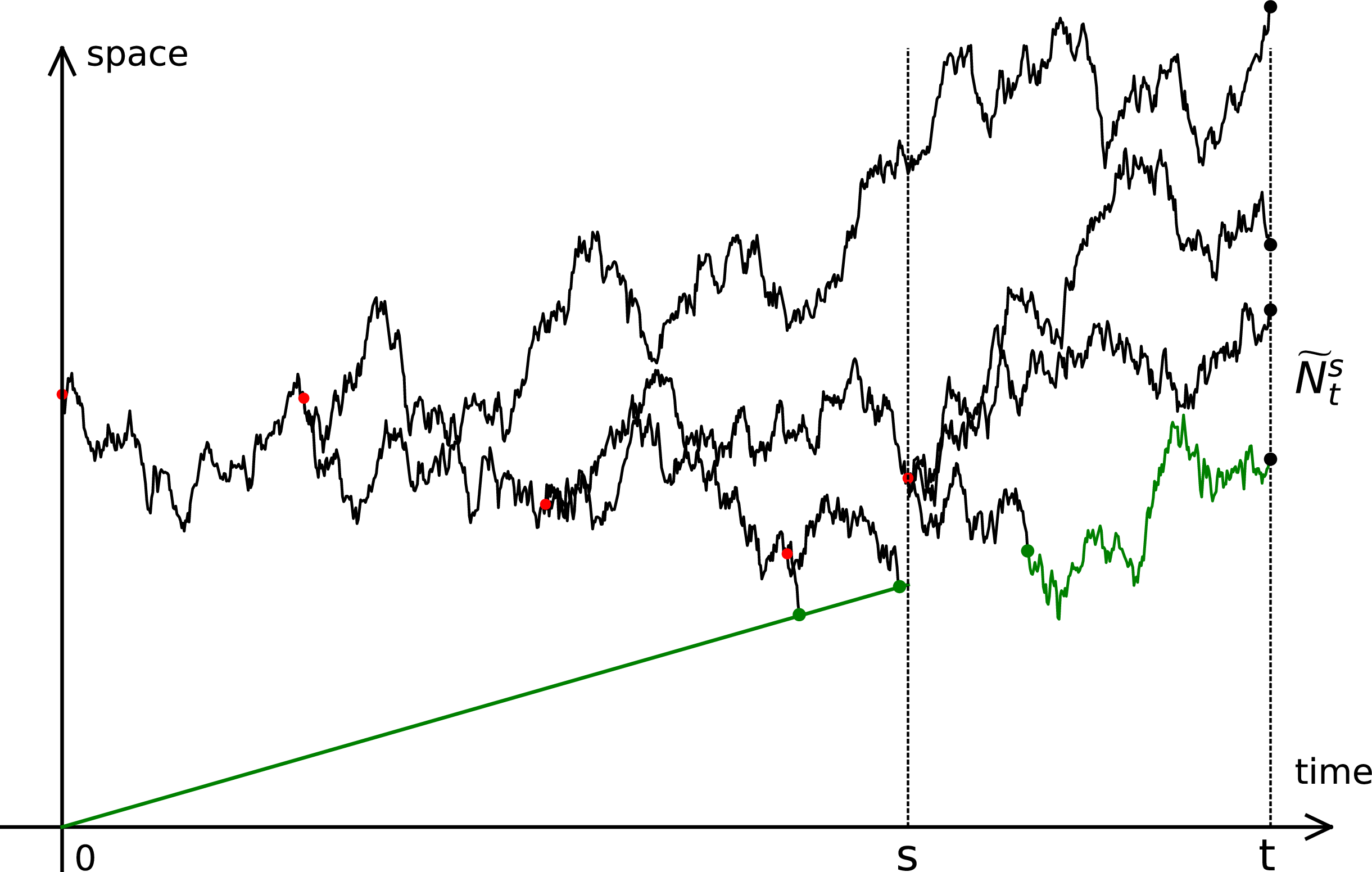
indicates that u is a descendant of v (see Figure 2). Notice that the set
$u>v$
indicates that u is a descendant of v (see Figure 2). Notice that the set $\widetilde{N}^s_t$
contains all the particles alive at time t that do not hit the line segment
$\widetilde{N}^s_t$
contains all the particles alive at time t that do not hit the line segment $\{(y,r)\colon y =\rho r,\, 0\leq r\leq s \}$
. For convenience, define
$\{(y,r)\colon y =\rho r,\, 0\leq r\leq s \}$
. For convenience, define $M_t \,:\!=\, \max\{X_u(t)\colon u\in N_t \} - m_t$
and
$M_t \,:\!=\, \max\{X_u(t)\colon u\in N_t \} - m_t$
and $\widetilde{M}_t \,:\!=\, \max\{X_u(t)\colon u\in \widetilde{N}_t \} - m_t$
. Then
$\widetilde{M}_t \,:\!=\, \max\{X_u(t)\colon u\in \widetilde{N}_t \} - m_t$
. Then $M_t = \mathbf{M}_t - m_t$
and
$M_t = \mathbf{M}_t - m_t$
and $\widetilde{M}_t = \widetilde{\mathbf{M}}_t - m_t$
. Similarly, define
$\widetilde{M}_t = \widetilde{\mathbf{M}}_t - m_t$
. Similarly, define
 \begin{equation} \widetilde{M}_t^s \,:\!=\, \max\{X_u(t)\colon u\in \widetilde{N}^s_t\} - m_t.\end{equation}
The truncated absorption barrier.
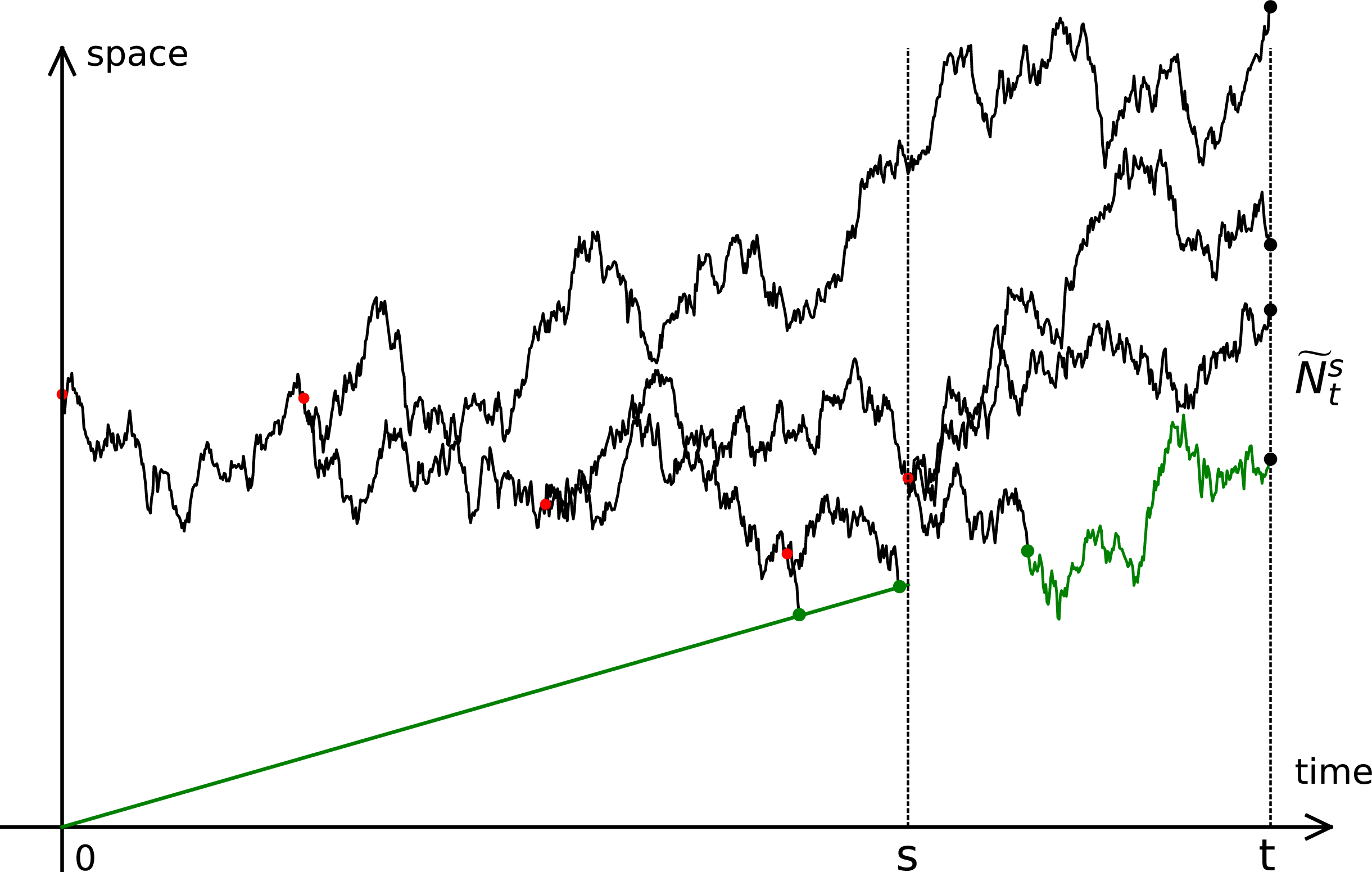
Figure 2 Long description
The graph illustrates branching Brownian motion with the truncated absorption barrier. The x-axis represents time, while the y-axis represents space. The absorption barrier is a segment that exists only up to some fixed time s. The particles are absorbed upon hitting this segment.
In the proof of Theorem 1.1, we need the following two lemmas, whose proofs are postponed to Sections 3 and 4. First, as in [Reference Arguin, Bovier and Kistler3], we consider the time $R_T>0$
. However, in this paper, we require that there exists some
$R_T>0$
. However, in this paper, we require that there exists some $l>0$
such that
$l>0$
such that $R_T/T^{l}\uparrow \infty$
and
$R_T/T^{l}\uparrow \infty$
and $R_T/\sqrt{T}\downarrow 0$
as
$R_T/\sqrt{T}\downarrow 0$
as $T\uparrow\infty$
. We truncate the absorption barrier at time
$T\uparrow\infty$
. We truncate the absorption barrier at time $R_T$
and will show that the empirical distribution of
$R_T$
and will show that the empirical distribution of $\widetilde{M}_t^{R_T}$
converges almost surely.
$\widetilde{M}_t^{R_T}$
converges almost surely.
Lemma 2.1. Let $R_T/T^l \uparrow\infty$
as
$R_T/T^l \uparrow\infty$
as $T\uparrow\infty$
for some
$T\uparrow\infty$
for some $l>0$
but with
$l>0$
but with $R_T = o(\sqrt{T})$
. Then, for any
$R_T = o(\sqrt{T})$
. Then, for any $x>0$
and
$x>0$
and $z\in\mathbb{R}$
,
$z\in\mathbb{R}$
,
 \begin{equation} \lim_{T\uparrow\infty}\frac{1}{T}\int_0^T\mathbf{1}_{\{\widetilde{M}_t^{R_T}\leq z\}}\,\mathrm{d}t = \exp\!\big\{{-}C_*\widetilde{Z}_{\infty}{\mathrm{e}}^{-\sqrt{2}z}\big\}, \quad \mathbb{P}_x\mbox{-a.s.} \end{equation}
Remark 2.1. In [Reference Yang and Zhu20], the absorption barrier was truncated at time s and the set $\widetilde{N}_t^s$
was used to approximate
$\widetilde{N}_t^s$
was used to approximate $\widetilde{N}_t$
. Following a similar approach, we can show that
$\widetilde{N}_t$
. Following a similar approach, we can show that
 \begin{equation*} \lim_{T\uparrow\infty}\frac{1}{T}\int_0^T\mathbf{1}_{\{\widetilde{M}_t^{s}\leq z\}}\,\mathrm{d}t = \exp\!\big\{{-}C_*\widetilde{Z}_{\infty}^s{\mathrm{e}}^{-\sqrt{2}z}\big\}, \quad \mathbb{P}_x\mbox{-a.s.}, \end{equation*}
where $\widetilde{Z}_{\infty}^s = \lim_{t\uparrow\infty}\sum_{u\in\widetilde{N}_t^s}(\sqrt{2}t-X_u(t)){\mathrm{e}}^{\sqrt{2}(X_u(t)-\sqrt{2}t)}$
and
$\widetilde{Z}_{\infty}^s = \lim_{t\uparrow\infty}\sum_{u\in\widetilde{N}_t^s}(\sqrt{2}t-X_u(t)){\mathrm{e}}^{\sqrt{2}(X_u(t)-\sqrt{2}t)}$
and $\lim_{s\uparrow\infty}\widetilde{Z}_{\infty}^s = \widetilde{Z}_{\infty}$
. Consequently,
$\lim_{s\uparrow\infty}\widetilde{Z}_{\infty}^s = \widetilde{Z}_{\infty}$
. Consequently,
 \begin{equation*} \lim_{s\uparrow\infty}\lim_{T\uparrow\infty}\frac{1}{T}\int_0^T\mathbf{1}_{\{\widetilde{M}_t^{s}\leq z\}}\,\mathrm{d}t = \exp\!\big\{{-}C_*\widetilde{Z}_{\infty}{\mathrm{e}}^{-\sqrt{2}z}\big\}, \quad \mathbb{P}_x\mbox{-a.s.} \end{equation*}
However, establishing Theorem 1.1 by interchanging the order of limits presents difficulties. To circumvent this, we replace the fixed truncation time s with a T-dependent quantity $R_T$
. Since
$R_T$
. Since $\widetilde{M}_t \leq \widetilde{M}^{R_T}_t$
, it follows that
$\widetilde{M}_t \leq \widetilde{M}^{R_T}_t$
, it follows that
 \begin{equation*} \liminf_{T\uparrow\infty}\frac{1}{T}\int_0^T\mathbf{1}_{\{\widetilde{M}_t\leq z\}}\,\mathrm{d}t \geq \exp\!\big\{{-}C_*\widetilde{Z}_{\infty}{\mathrm{e}}^{-\sqrt{2}z}\big\}, \quad \mathbb{P}_x\mbox{-a.s.} \end{equation*}
Next, we consider the difference between $\widetilde{M}_t$
and
$\widetilde{M}_t$
and $\widetilde{M}_t^{R_T}$
. For
$\widetilde{M}_t^{R_T}$
. For $s<t$
, define
$s<t$
, define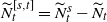 $\widetilde{N}_t^{[s,t]} = \widetilde{N}_t^s - \widetilde{N}_t$
, which represents the set of particles at time t whose ancestors are not absorbed before time s but hit the absorption barrier between time s and t. Define
$\widetilde{N}_t^{[s,t]} = \widetilde{N}_t^s - \widetilde{N}_t$
, which represents the set of particles at time t whose ancestors are not absorbed before time s but hit the absorption barrier between time s and t. Define
 \begin{equation*} \widetilde{M}_t^{[s,t]} \,:\!=\, \max\big\{X_u(t)\colon u\in\widetilde{N}_t^{[s,t]}\big\} - m_t.\end{equation*}
The following lemma provides the convergence of the empirical distribution of $\widetilde{M}_t^{[s,t]}$
.
$\widetilde{M}_t^{[s,t]}$
.
Lemma 2.2. For $\varepsilon>0$
and
$\varepsilon>0$
and $R_T$
as in Lemma 2.1,
$R_T$
as in Lemma 2.1,
 \begin{equation} \limsup_{T\uparrow\infty}\frac{1}{T}\int_{\varepsilon T}^T\mathbf{1}_{\{\widetilde{M}_t^{[R_T,t]} \gt z\}}\,\mathrm{d}t = 0, \quad \mathbb{P}_x\mbox{-a.s.} \end{equation}
Remark 2.2. This lemma shows that the particles whose ancestors were absorbed during the interval $[R_T,t]$
do not contribute to the maximum. Moreover, it serves as the key to establishing the converse direction of equation (1.3).
$[R_T,t]$
do not contribute to the maximum. Moreover, it serves as the key to establishing the converse direction of equation (1.3).
Proof of Theorem
1.1. Note that $\widetilde{N}_t \subset \widetilde{N}_t^{R_T}$
. Hence,
$\widetilde{N}_t \subset \widetilde{N}_t^{R_T}$
. Hence, $\widetilde{M}_t \leq \widetilde{M}^{R_T}_t$
and then
$\widetilde{M}_t \leq \widetilde{M}^{R_T}_t$
and then $\mathbf{1}_{\{\widetilde{M}_t \leq z\}} \geq \mathbf{1}_{\{\widetilde{M}^{R_T}_t \leq z\}}$
. By Lemma 2.1,
$\mathbf{1}_{\{\widetilde{M}_t \leq z\}} \geq \mathbf{1}_{\{\widetilde{M}^{R_T}_t \leq z\}}$
. By Lemma 2.1,
 \begin{equation*} \liminf_{T\uparrow\infty}\frac{1}{T}\int_0^T\mathbf{1}_{\{\widetilde{M}_t\leq z\}}\,\mathrm{d}t \geq \exp\!\big\{{-}C_*\widetilde{Z}_{\infty}{\mathrm{e}}^{-\sqrt{2}z}\big\}, \quad \mathbb{P}_x\mbox{-a.s.} \end{equation*}
Since $\mathbf{1}_{\{\widetilde{M}_t\leq z\}} + \mathbf{1}_{\{\widetilde{M}_t \gt z\}} = 1$
, we have
$\mathbf{1}_{\{\widetilde{M}_t\leq z\}} + \mathbf{1}_{\{\widetilde{M}_t \gt z\}} = 1$
, we have
 \begin{equation*} \limsup_{T\uparrow\infty}\frac{1}{T}\int_0^T\mathbf{1}_{\{\widetilde{M}_t \gt z\}}\,\mathrm{d}t \leq 1-\exp\!\big\{{-}C_*\widetilde{Z}_{\infty}{\mathrm{e}}^{-\sqrt{2}z}\big\}, \quad \mathbb{P}_x\mbox{-a.s.} \end{equation*}
To prove Theorem 1.1, it suffices to show that
 \begin{equation} \liminf_{T\uparrow\infty}\frac{1}{T}\int_0^T\mathbf{1}_{\{\widetilde{M}_t \gt z\}}\,\mathrm{d}t \geq 1-\exp\!\big\{{-}C_*\widetilde{Z}_{\infty}{\mathrm{e}}^{-\sqrt{2}z}\big\}, \quad \mathbb{P}_x\mbox{-a.s.} \end{equation}
Since $\widetilde{M}_t^s = \max\big\{\widetilde{M}_t,\widetilde{M}_t^{[s,t]}\big\}$
, we have
$\widetilde{M}_t^s = \max\big\{\widetilde{M}_t,\widetilde{M}_t^{[s,t]}\big\}$
, we have $\mathbf{1}_{\{\widetilde{M}_t^s \gt z\}} \leq \mathbf{1}_{\{\widetilde{M}_t \gt z\}} + \mathbf{1}_{\{\widetilde{M}_t^{[s,t]} \gt z\}}$
, that is,
$\mathbf{1}_{\{\widetilde{M}_t^s \gt z\}} \leq \mathbf{1}_{\{\widetilde{M}_t \gt z\}} + \mathbf{1}_{\{\widetilde{M}_t^{[s,t]} \gt z\}}$
, that is, $\mathbf{1}_{\{\widetilde{M}_t \gt z\}} \geq \mathbf{1}_{\{\widetilde{M}_t^s \gt z\}} - \mathbf{1}_{\{\widetilde{M}_t^{[s,t]} \gt z\}}$
. For
$\mathbf{1}_{\{\widetilde{M}_t \gt z\}} \geq \mathbf{1}_{\{\widetilde{M}_t^s \gt z\}} - \mathbf{1}_{\{\widetilde{M}_t^{[s,t]} \gt z\}}$
. For $s=R_T$
, we have
$s=R_T$
, we have
 \begin{equation} \liminf_{T\uparrow\infty}\frac{1}{T}\int_{\varepsilon T}^T\mathbf{1}_{\{\widetilde{M}_t \gt z\}}\,\mathrm{d}t \geq \liminf_{T\uparrow\infty}\frac{1}{T}\int_{\varepsilon T}^T\mathbf{1}_{\big\{\widetilde{M}_t^{R_T} \gt z\big\}}\,\mathrm{d}t - \limsup_{T\uparrow\infty}\frac{1}{T}\int_{\varepsilon T}^T\mathbf{1}_{\big\{\widetilde{M}_t^{[R_T,t]} \gt z\big\}}\,\mathrm{d}t. \end{equation}
For any $\varepsilon>0$
, by (2.7) and Lemma 2.2,
$\varepsilon>0$
, by (2.7) and Lemma 2.2,
 \begin{equation*} \liminf_{T\uparrow\infty}\frac{1}{T}\int_0^T\mathbf{1}_{\{\widetilde{M}_t \gt z\}}\,\mathrm{d}t \geq \liminf_{T\uparrow\infty}\frac{1}{T}\int_{\varepsilon T}^T\mathbf{1}_{\{\widetilde{M}_t \gt z\}}\,\mathrm{d}t \geq \liminf_{T\uparrow\infty}\frac{1}{T}\int_{\varepsilon T}^T\mathbf{1}_{\big\{\widetilde{M}_t^{R_T} \gt z\big\}}\,\mathrm{d}t. \end{equation*}
Therefore,
 \begin{align*} \liminf_{T\uparrow\infty}\frac{1}{T}\int_0^T\mathbf{1}_{\{\widetilde{M}_t \gt z\}}\,\mathrm{d}t & \geq \liminf_{T\uparrow\infty}\bigg(\frac{1}{T}\int_{0}^T\mathbf{1}_{\big\{\widetilde{M}_t^{R_T} \gt z\big\}}\,\mathrm{d}t - \frac{1}{T}\int_{0}^{\varepsilon T}\mathbf{1}_{\big\{\widetilde{M}_t^{R_T} \gt z\big\}}\,\mathrm{d}t\bigg) \\ & \geq \liminf_{T\uparrow\infty}\frac{1}{T}\int_{0}^T\mathbf{1}_{\big\{\widetilde{M}_t^{R_T} \gt z\big\}}\,\mathrm{d}t - \varepsilon \\ & \geq 1 - \exp\!\big\{{-}C_*\widetilde{Z}_{\infty}{\mathrm{e}}^{-\sqrt{2}z}\big\} - \varepsilon, \end{align*}
where the last inequality follows from Lemma 2.1. Let $\varepsilon \downarrow 0$
, then the inequality (2.6) holds. This completes the proof.
$\varepsilon \downarrow 0$
, then the inequality (2.6) holds. This completes the proof.
3. Proof of Lemma 2.1
In this section we prove Lemma 2.1, which states that for any $x>0$
and
$x>0$
and $z\in\mathbb{R}$
,
$z\in\mathbb{R}$
,
 \begin{equation*} \lim_{T\uparrow\infty}\frac{1}{T}\int_0^T\mathbf{1}_{\big\{\widetilde{M}_t^{R_T}\leq z\big\}}\,\mathrm{d}t = \exp\!\big\{{-}C_*\widetilde{Z}_{\infty}{\mathrm{e}}^{-\sqrt{2}z}\big\}, \quad \mathbb{P}_x\mbox{-a.s.}\end{equation*}
Let $\mathcal{D} = [d,D]$
with
$\mathcal{D} = [d,D]$
with $-\infty < d < D < \infty$
, which is a compact set. Similarly to [Reference Arguin, Bovier and Kistler3], this lemma follows from the following two lemmas.
$-\infty < d < D < \infty$
, which is a compact set. Similarly to [Reference Arguin, Bovier and Kistler3], this lemma follows from the following two lemmas.
Lemma 3.1. For $\varepsilon>0$
and
$\varepsilon>0$
and $R_T$
as in Lemma 2.1, and for any
$R_T$
as in Lemma 2.1, and for any $s\in [\varepsilon,1]$
,
$s\in [\varepsilon,1]$
,
 \begin{equation*} \lim_{T\uparrow\infty}\mathbb{P}_x\big[\widetilde{M}^{R_T}_{T\cdot s}\in\mathcal{D}\mid\mathcal{F}_{R_T}\big] = \int_{\mathcal{D}}\mathrm{d}\big(\!\exp\!\big\{{-}C_*\widetilde{Z}_{\infty}{\mathrm{e}}^{-\sqrt{2}z}\big\}\big), \quad \mathbb{P}_x\mbox{-a.s.} \end{equation*}
Lemma 3.2. For $\varepsilon>0$
and
$\varepsilon>0$
and $R_T$
as in Lemma 2.1,
$R_T$
as in Lemma 2.1,
 \begin{equation*} \lim_{T\uparrow\infty}\frac{1}{T}\int_{\varepsilon T}^T\Big(\mathbf{1}_{\big\{\widetilde{M}^{R_T}_t \in \mathcal{D}\big\}} - \mathbb{P}_x\big[\widetilde{M}^{R_T}_{t}\in\mathcal{D}\mid\mathcal{F}_{R_T}\big]\Big)\,\mathrm{d}t = 0, \quad \mathbb{P}_x\mbox{-a.s.} \end{equation*}
Proof of Lemma 3.1. First, we write
 \begin{equation*} \mathbb{P}_x\big[\widetilde{M}^{R_T}_{T\cdot s}\in\mathcal{D}\mid\mathcal{F}_{R_T}\big] = \mathbb{P}_x\big[\widetilde{M}^{R_T}_{T\cdot s} \leq D\mid\mathcal{F}_{R_T}\big] - \mathbb{P}_x\big[\widetilde{M}^{R_T}_{T\cdot s} \leq d\mid\mathcal{F}_{R_T}\big]. \end{equation*}
We only need to show the almost-sure convergence of the first term. Recalling the definitions in (2.1), (2.2), and (2.3), then
 \begin{align*} \mathbb{P}_x\big[\widetilde{M}^{R_T}_{T\cdot s} \leq D\mid\mathcal{F}_{R_T}\big] & = \prod_{u\in\widetilde{N}_{R_T}}\mathbb{P}_x\big[X_u(R_T) + M_{T\cdot s - R_T}(u) + m_{T\cdot s - R_T} \leq D + m_{T\cdot s}\mid\mathcal{F}_{R_T}\big] \\ & = \prod_{u\in\widetilde{N}_{R_T}}\big(1 - \mathbb{P}_x\big[M_{T\cdot s - R_T}(u) \gt D - X_u(R_T) + \sqrt{2}R_T + o_T(1)\mid\mathcal{F}_{R_T}\big]\big) \end{align*}
where, given $\mathcal{F}_{R_T}$
,
$\mathcal{F}_{R_T}$
, $\{M_{T\cdot s - R_T}(u), u\in \widetilde{N}_{R_T}\}$
are independent and have the same distribution as
$\{M_{T\cdot s - R_T}(u), u\in \widetilde{N}_{R_T}\}$
are independent and have the same distribution as $\{M_{T\cdot s - R_T}, \mathbb{P}_0\}$
. Note that
$\{M_{T\cdot s - R_T}, \mathbb{P}_0\}$
. Note that $o_T(1)\rightarrow 0$
as
$o_T(1)\rightarrow 0$
as $T\rightarrow \infty$
. After time
$T\rightarrow \infty$
. After time $R_T$
, there is no absorption barrier when
$R_T$
, there is no absorption barrier when $\widetilde{M}^{R_T}_{T\cdot s}$
is considered. Therefore, we can use a similar argument to [Reference Arguin, Bovier and Kistler3]. By [Reference Lalley and Sellke15, (20), p. 1055],
$\widetilde{M}^{R_T}_{T\cdot s}$
is considered. Therefore, we can use a similar argument to [Reference Arguin, Bovier and Kistler3]. By [Reference Lalley and Sellke15, (20), p. 1055],
 \begin{equation} \lim_{R_T\rightarrow\infty}\min_{u\in N_{R_T}}\big(\sqrt{2}R_T - X_u(R_T)\big) = +\infty \quad \mbox{a.s.} \end{equation}
Let $f(D, R_T) \,:\!=\, D - X_u(R_T) + \sqrt{2}R_T + o_T(1)$
. By [Reference Arguin, Bovier and Kistler3, Lemma 4], we have
$f(D, R_T) \,:\!=\, D - X_u(R_T) + \sqrt{2}R_T + o_T(1)$
. By [Reference Arguin, Bovier and Kistler3, Lemma 4], we have
 \begin{equation*} \mathbb{P}_x\big[M_{T\cdot s - R_T}(u) \gt f(D, R_T)\mid\mathcal{F}_{R_T}\big] = C_*(1+o_r(1))(1+o_T(1))\,f(D, R_T){\mathrm{e}}^{-\sqrt{2} f(D, R_T) }, \end{equation*}
and by (3.1) this probability tends to zero uniformly for $u\in\widetilde{N}_{R_T}$
as
$u\in\widetilde{N}_{R_T}$
as $T\rightarrow\infty$
. Hence,
$T\rightarrow\infty$
. Hence,
 \begin{align*} \mathbb{P}_x\big[\widetilde{M}^{R_T}_{T\cdot s} \leq D\mid\mathcal{F}_{R_T}\big] & = \exp\!\Bigg(\sum_{u\in\widetilde{N}_{R_T}}\log\big(1 - \mathbb{P}_x\big[M_{T\cdot s - R_T}(u) \gt f(D, R_T)\mid\mathcal{F}_{R_T}\big]\big)\Bigg) \\ & = \exp\!\Bigg({-}\sum_{u\in\widetilde{N}_{R_T}}C_*(1+o_r(1))(1+o_T(1))^2\,f(D,R_T){\mathrm{e}}^{-\sqrt{2}f(D,R_T)}\Bigg). \end{align*}
By the results on the additive martingale of BBM and the ‘derivative martingale’ of BBM with absorption given in [Reference Kyprianou14, Theorem 1(ii)] and [Reference Yang and Zhu20, Theorem 2.1], respectively, we have
 \begin{equation*} \lim_{T\uparrow\infty}\sum_{u\in\widetilde{N}_{R_T}}D{\mathrm{e}}^{-\sqrt{2}\big(\sqrt{2}R_T-X_u(R_T)\big)} \leq \lim_{T\uparrow\infty}\sum_{u\in N_{R_T}}D{\mathrm{e}}^{-\sqrt{2}\big(\sqrt{2}R_T-X_u(R_T)\big)} = 0 \end{equation*}
and
 \begin{equation*} \lim_{T\uparrow\infty}\sum_{u\in\widetilde{N}_{R_T}}\big(\sqrt{2}R_T-X_u(R_T)\big){\mathrm{e}}^{-\sqrt{2}(\sqrt{2}R_T-X_u(R_T))} = \widetilde{Z}_{\infty}. \end{equation*}
Therefore, we get
 \begin{align*} \lim_{T\uparrow\infty}\mathbb{P}_x\big[\widetilde{M}^{R_T}_{T\cdot s} \leq D\mid\mathcal{F}_{R_T}\big] & = \exp\!\Bigg({-}C_*(1+o_r(1))\lim_{T\uparrow\infty}\sum_{u\in\widetilde{N}_{R_T}}f(D,R_T){\mathrm{e}}^{-\sqrt{2}f(D,R_T)}\Bigg) \\ & = \exp\!\big({-}C_*(1+o_r(1)){\mathrm{e}}^{-\sqrt{2}D}\widetilde{Z}_{\infty}\big). \end{align*}
Letting $r\uparrow\infty$
yields
$r\uparrow\infty$
yields $\lim_{T\uparrow\infty}\mathbb{P}_x\big[\widetilde{M}^{R_T}_{T\cdot s} \leq D\mid\mathcal{F}_{R_T}\big] = \exp\!\big({-}C_*{\mathrm{e}}^{-\sqrt{2}D}\widetilde{Z}_{\infty}\big)$
. This completes the proof of Lemma 3.1.
$\lim_{T\uparrow\infty}\mathbb{P}_x\big[\widetilde{M}^{R_T}_{T\cdot s} \leq D\mid\mathcal{F}_{R_T}\big] = \exp\!\big({-}C_*{\mathrm{e}}^{-\sqrt{2}D}\widetilde{Z}_{\infty}\big)$
. This completes the proof of Lemma 3.1.
Proof of Lemma
3.2. Since, after time $R_T$
, the particle behaves as a branching Brownian motion, most of the proof of [Reference Arguin, Bovier and Kistler3, Theorem 3] is valid for Lemma 3.2. Now we provide the details.
$R_T$
, the particle behaves as a branching Brownian motion, most of the proof of [Reference Arguin, Bovier and Kistler3, Theorem 3] is valid for Lemma 3.2. Now we provide the details.
Fix $x>0$
. For
$x>0$
. For $\gamma>0$
,
$\gamma>0$
, $0\leq s \leq t$
, define
$0\leq s \leq t$
, define $F_{\gamma,t}(s) \,:\!=\, x + ({s}/{t})m_t - \min\{s^{\gamma}, (t-s)^{\gamma} \}$
. Choose
$F_{\gamma,t}(s) \,:\!=\, x + ({s}/{t})m_t - \min\{s^{\gamma}, (t-s)^{\gamma} \}$
. Choose $0<\alpha<\frac12<\beta<1$
. We say that a particle
$0<\alpha<\frac12<\beta<1$
. We say that a particle $u\in N_t$
is localized in the time t-tube during the interval
$u\in N_t$
is localized in the time t-tube during the interval $(r,t-r)$
if and only if
$(r,t-r)$
if and only if $F_{\beta,t}(s) \leq X_u(s) \leq F_{\alpha,t}(s)$
for all
$F_{\beta,t}(s) \leq X_u(s) \leq F_{\alpha,t}(s)$
for all $s\in (r,t-r)$
. Otherwise, we say that it is not localized. By [Reference Arguin, Bovier and Kistler3, Proposition 6], for given
$s\in (r,t-r)$
. Otherwise, we say that it is not localized. By [Reference Arguin, Bovier and Kistler3, Proposition 6], for given $\mathcal{D}=[d,D]$
there exist
$\mathcal{D}=[d,D]$
there exist $r_0, \delta>0$
depending on
$r_0, \delta>0$
depending on $\alpha$
,
$\alpha$
, $\beta$
, and
$\beta$
, and $\mathcal{D}$
such that, for
$\mathcal{D}$
such that, for $r\geq r_0$
,
$r\geq r_0$
,
 \begin{multline} \sup\nolimits_{t\geq 3r}\mathbb{P}_x[\text{there exists}\ u\in N_t\colon X_u(t) - m_t\in\mathcal{D} \mbox{ but }\textit{u} \ \textrm{is} \ \textit{not localized} \ \textrm{during } (r,t-r)] \\ \leq \exp\{-r^{\delta}\}. \end{multline}
Choose $r_T = (20\ln T)^{1/\delta}$
. For any
$r_T = (20\ln T)^{1/\delta}$
. For any $t\in (R_T,T)$
, define
$t\in (R_T,T)$
, define
 \begin{equation*} \widetilde{M}_{t,\mathrm{loc}}^{R_T} \,:\!=\, \max\big\{X_u(t)\colon u\in\widetilde{N}_t^{R_T},\, u\ \text{is} \textit{ localized} \mbox{ during } (r_T,t-r_T) \big\} - m_t. \end{equation*}
Then, we have
 \begin{align*} & \mathbb{P}_x\big(\big\{\widetilde{M}_{t}^{R_T}\in\mathcal{D}\big\} \setminus \big\{\widetilde{M}_{t,\mathrm{loc}}^{R_T}\in\mathcal{D}\big\}\big) \\ & \quad \leq \mathbb{P}_x\big[\text{there exists}\ u\in\widetilde{N}_t^{R_T}\colon X_u(t) - m_t\in\mathcal{D} \mbox{ but}\, \textit{u}\, \mbox{is}\, \textit{not localized}\, \mbox{during } (r_T,t-r_T) \big] \\ & \quad \leq \mathbb{P}_x[\text{there exists}\ u\in N_t\colon X_u(t) - m_t \in \mathcal{D} \mbox{ but}\, \textit{u}\, \mbox{is}\, \textit{not localized}\, \mbox{during } (r_T,t-r_T)]. \end{align*}
Hence, (3.2) implies that $\mathbb{P}_x\big(\big\{\widetilde{M}_{t}^{R_T}\in\mathcal{D}\big\} \setminus \big\{\widetilde{M}_{t,\mathrm{loc}}^{R_T}\in\mathcal{D}\big\}\big) \leq {1}/{T^{20}}$
. Since
$\mathbb{P}_x\big(\big\{\widetilde{M}_{t}^{R_T}\in\mathcal{D}\big\} \setminus \big\{\widetilde{M}_{t,\mathrm{loc}}^{R_T}\in\mathcal{D}\big\}\big) \leq {1}/{T^{20}}$
. Since $\big\{\widetilde{M}_{t}^{R_T}\geq D\big\} \cap \big\{\widetilde{M}_{t,\mathrm{loc}}^{R_T}\in\mathcal{D}\big\} \neq \emptyset$
, the inequality
$\big\{\widetilde{M}_{t}^{R_T}\geq D\big\} \cap \big\{\widetilde{M}_{t,\mathrm{loc}}^{R_T}\in\mathcal{D}\big\} \neq \emptyset$
, the inequality $\mathbb{P}_x\big(\widetilde{M}_{t}^{R_T}\in\mathcal{D}\big) - \mathbb{P}_x\big(\widetilde{M}_{t,loc}^{R_T} \in \mathcal{D}\big) \geq 0$
is not true. The same issue exists in [Reference Arguin, Bovier and Kistler3, (4.11)]. However, we have the following claim, with a slight modification from [Reference Arguin, Bovier and Kistler1, Theorems 2.3 and 2.5].
$\mathbb{P}_x\big(\widetilde{M}_{t}^{R_T}\in\mathcal{D}\big) - \mathbb{P}_x\big(\widetilde{M}_{t,loc}^{R_T} \in \mathcal{D}\big) \geq 0$
is not true. The same issue exists in [Reference Arguin, Bovier and Kistler3, (4.11)]. However, we have the following claim, with a slight modification from [Reference Arguin, Bovier and Kistler1, Theorems 2.3 and 2.5].
Claim A. There exist $r_0, \delta>0$
depending on
$r_0, \delta>0$
depending on $\alpha$
,
$\alpha$
, $\beta$
, and D such that, for
$\beta$
, and D such that, for $r\geq r_0$
,
$r\geq r_0$
,
 \begin{multline} \sup\nolimits_{t\geq 3r}\mathbb{P}_x[\text{there exists}\ u\in N_t\colon X_u(t) - m_t \geq D \mbox{ but}\, \textit{u}\, \mbox{is}\, \text{not localized}\, \mbox{during } (r,t-r)] \\ \leq \exp\{-r^{\delta}\}. \end{multline}
We prove this claim in Appendix A.
Therefore,
 \begin{align*} & \mathbb{P}_x\big(\big\{\widetilde{M}_{t,\mathrm{loc}}^{R_T}\in\mathcal{D}\big\} \setminus \big\{\widetilde{M}_{t}^{R_T}\in\mathcal{D}\big\}\big) \\ & \quad \leq \mathbb{P}_x[\text{there exists}\ u\in N_t\colon X_u(t) - m_t \geq D \mbox{ but}\, \textit{u}\, \mbox{is}\, \textit{not localized}\, \mbox{during } (r_T,t-r_T)] \\ & \quad \leq {1}/{T^{20}}. \end{align*}
Let
 \begin{align*} \text{Rest}_{\varepsilon,\mathcal{D}}(T) & \,:\!=\, \frac{1}{T}\int_{\varepsilon T}^T\bigg(\mathbf{1}_{\big\{\widetilde{M}^{R_T}_t\in\mathcal{D}\big\}} - \mathbb{P}_x\big[\widetilde{M}^{R_T}_{t}\in\mathcal{D}\mid\mathcal{F}_{R_T}\big]\bigg)\,\mathrm{d}t, \\ \text{Rest}_{\varepsilon,\mathcal{D}}^{\mathrm{loc}}(T) & \,:\!=\, \frac{1}{T}\int_{\varepsilon T}^T\bigg(\mathbf{1}_{\big\{\widetilde{M}^{R_T}_{t,\mathrm{loc}}\in\mathcal{D}\big\}} - \mathbb{P}_x\big[\widetilde{M}^{R_T}_{t,\mathrm{loc}}\in\mathcal{D}\mid\mathcal{F}_{R_T}\big]\bigg)\,\mathrm{d}t. \end{align*}
Using an argument similar to that in the proof of [Reference Arguin, Bovier and Kistler3, Lemma 7], we have
 \begin{equation} \lim_{T\uparrow\infty}\big(\text{Rest}_{\varepsilon,\mathcal{D}}(T) - \text{Rest}_{\varepsilon,\mathcal{D}}^{\mathrm{loc}}(T)\big) = 0, \quad \mathbb{P}_x\mbox{-a.s.} \end{equation}
For completeness, we give the details here. We have
 \begin{align*} \text{Rest}_{\varepsilon,\mathcal{D}}(T) - \text{Rest}_{\varepsilon,\mathcal{D}}^{\mathrm{loc}}(T) & = \frac{1}{T}\int_{\varepsilon T}^T\big(\mathbf{1}_{\big\{\widetilde{M}^{R_T}_t\in\mathcal{D}\big\}} - \mathbf{1}_{\big\{\widetilde{M}^{R_T}_{t,\mathrm{loc}}\in\mathcal{D}\big\}}\big)\,\mathrm{d}t \\ & \quad - \frac{1}{T}\int_{\varepsilon T}^T\big(\mathbb{P}_x\big[\widetilde{M}^{R_T}_{t}\in\mathcal{D} \mid \mathcal{F}_{R_T}\big] - \mathbb{P}_x\big[\widetilde{M}^{R_T}_{t,\mathrm{loc}}\in\mathcal{D} \mid \mathcal{F}_{R_T}\big]\big)\,\mathrm{d}t \\ & \,=\!:\, \mathrm{I}_{T,\varepsilon} - \mathrm{II}_{T,\varepsilon}. \end{align*}
Notice that
 \begin{align*} & \mathbb{E}_x\bigg|\frac{1}{T}\int_{\varepsilon T}^T\bigg(\mathbf{1}_{\big\{\widetilde{M}^{R_T}_t\in\mathcal{D}\big\}} - \mathbf{1}_{\big\{\widetilde{M}^{R_T}_{t,\mathrm{loc}}\in\mathcal{D}\big\}}\bigg)\,\mathrm{d}t\bigg| \\ & \leq \frac{1}{T}\int_{\varepsilon T}^T\mathbb{E}_x\big|\mathbf{1}_{\big\{\widetilde{M}^{R_T}_t\in\mathcal{D}\big\}} - \mathbf{1}_{\big\{\widetilde{M}^{R_T}_{t,\mathrm{loc}}\in\mathcal{D}\big\}}\big|\,\mathrm{d}t \\ & \leq \frac{1}{T}\int_{\varepsilon T}^T\big[\mathbb{P}_x\big(\big\{\widetilde{M}_{t}^{R_T}\in\mathcal{D}\big\} \setminus \big\{\widetilde{M}_{t,\mathrm{loc}}^{R_T}\in\mathcal{D}\big\}\big) + \mathbb{P}_x\big(\big\{\widetilde{M}_{t,\mathrm{loc}}^{R_T}\in\mathcal{D}\big\} \setminus \big\{\widetilde{M}_{t}^{R_T}\in\mathcal{D}\big\}\big)\big]\,\mathrm{d}t \leq \frac{2}{T^{20}}. \end{align*}
Then, it follows from Markov’s inequality that
 \begin{equation*} \mathbb{P}(|\mathrm{I}_{T,\varepsilon}| \gt \delta) \leq \frac{1}{\delta}\mathbb{E}_x\bigg|\frac{1}{T}\int_{\varepsilon T}^T\bigg( \mathbf{1}_{\big\{\widetilde{M}^{R_T}_t\in\mathcal{D}\big\}} - \mathbf{1}_{\big\{\widetilde{M}^{R_T}_{t,\mathrm{loc}}\in\mathcal{D}\big\}}\bigg)\,\mathrm{d}t\bigg| \leq \frac{2}{\delta T^{20}}, \end{equation*}
which is summable over T (noticing that we may take $T\in\mathbb{N}$
). Hence, by the Borel–Cantelli lemma,
$T\in\mathbb{N}$
). Hence, by the Borel–Cantelli lemma, $\mathbb{P}(\{|\mathrm{I}_{T,\varepsilon}| \gt \delta\} \mbox{ infinitely often}) = 0$
. Since this holds for every
$\mathbb{P}(\{|\mathrm{I}_{T,\varepsilon}| \gt \delta\} \mbox{ infinitely often}) = 0$
. Since this holds for every $\delta>0$
, it follows that
$\delta>0$
, it follows that $\lim_{T\uparrow\infty}\mathrm{I}_{T,\varepsilon} = 0$ $\mathbb{P}$
-a.s. The proof of
$\mathbb{P}$
-a.s. The proof of $\lim_{T\uparrow\infty}\mathrm{II}_{T,\varepsilon} = 0$
is analogous. Equation (3.4) is therefore established. Then, it suffices to prove that
$\lim_{T\uparrow\infty}\mathrm{II}_{T,\varepsilon} = 0$
is analogous. Equation (3.4) is therefore established. Then, it suffices to prove that $\lim_{T\uparrow\infty}\text{Rest}_{\varepsilon,\mathcal{D}}^{\mathrm{loc}}(T) = 0$
,
$\lim_{T\uparrow\infty}\text{Rest}_{\varepsilon,\mathcal{D}}^{\mathrm{loc}}(T) = 0$
, $\mathbb{P}_x$
-a.s.
$\mathbb{P}_x$
-a.s.
Define
 \begin{equation*} X_t^{\{D\}} \,:\!=\, \mathbf{1}_{\big\{\widetilde{M}^{R_T}_{t,\mathrm{loc}} \leq D\big\}} - \mathbb{P}_x\big[\widetilde{M}^{R_T}_{t,\mathrm{loc}} \leq D \mid \mathcal{F}_{R_T}\big], \qquad \widehat{C}_T(t,t') \,:\!=\, \mathbb{E}_x\big[X_t^{\{D\}}\cdot X_{t'}^{\{D\}}\big]. \end{equation*}
Then, we have
 \begin{align*} \text{Rest}_{\varepsilon,\mathcal{D}}^{\mathrm{loc}}(T) = \frac{1}{T}\int_{\varepsilon T}^T X_s^{\{D\}}\,\mathrm{d}s - \frac{1}{T}\int_{\varepsilon T}^T X_s^{\{d\}}\,\mathrm{d}s. \end{align*}
By [Reference Arguin, Bovier and Kistler3, Theorem 8], we only need to verify that both integrals satisfy the assumptions of this theorem. Once this is done, we can conclude that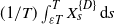 $({1}/{T})\int_{\varepsilon T}^T X_s^{\{D\}}\,\mathrm{d}s$
and
$({1}/{T})\int_{\varepsilon T}^T X_s^{\{D\}}\,\mathrm{d}s$
and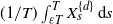 $({1}/{T})\int_{\varepsilon T}^T X_s^{\{d\}}\,\mathrm{d}s$
converge to 0 as
$({1}/{T})\int_{\varepsilon T}^T X_s^{\{d\}}\,\mathrm{d}s$
converge to 0 as $T\to\infty$
. By definition,
$T\to\infty$
. By definition, $|X_s^{\{D\}}|\leq 2$
almost surely for all
$|X_s^{\{D\}}|\leq 2$
almost surely for all $s>0$
, and
$s>0$
, and $\mathbb{E}[X_s^{\{D\}}] = 0$
. Hence, it is enough to check that
$\mathbb{E}[X_s^{\{D\}}] = 0$
. Hence, it is enough to check that
 \begin{equation*} \sum_{T=1}^{\infty}\frac{1}{T}\mathbb{E}\bigg[\bigg|\frac{1}{T}\int_{\varepsilon T}^T X_s^{\{D\}}\,\mathrm{d}s\bigg|^2\bigg] \lt \infty. \end{equation*}
Following the computations in [Reference Arguin, Bovier and Kistler3, (4.28) and (4.29)], we obtain
 \begin{align} & \sum_{T=1}^{\infty}\frac{1}{T}\mathbb{E}\bigg[\bigg|\frac{1}{T}\int_{\varepsilon T}^T X_s^{\{D\}}\,\mathrm{d}s\bigg|^2\bigg] \nonumber\\ & \qquad = 2\sum_{T=1}^{\infty}\frac{1}{T^3}\int_{\varepsilon T}^T\mathrm{d}s\int_s^T\mathrm{d}s'\widehat{C}_T(s,s') \nonumber\\ & \qquad = 2\sum_{T=1}^{\infty}\frac{1}{T^3}\int_{\varepsilon T}^T\mathrm{d}s\int_s^{s+T^{\xi}}\mathrm{d}s' \widehat{C}_T(s,s') + 2\sum_{T=1}^{\infty}\frac{1}{T^3}\int_{\varepsilon T}^T\mathrm{d}s\int_{s+T^{\xi}}^T\mathrm{d}s'\widehat{C}_T(s,s'), \end{align}
where $\xi\in(0,1)$
is a fixed constant. The first term in (3.5) is bounded by
$\xi\in(0,1)$
is a fixed constant. The first term in (3.5) is bounded by $2\sum_{T=1}^{\infty}({1}/{T^3})T\cdot T^{\xi}\cdot 1$
, which is finite. It remains to show that the second term in (3.5) is also finite. For this, it suffices to verify the validity of [Reference Arguin, Bovier and Kistler3, Theorem 9] for this
$2\sum_{T=1}^{\infty}({1}/{T^3})T\cdot T^{\xi}\cdot 1$
, which is finite. It remains to show that the second term in (3.5) is also finite. For this, it suffices to verify the validity of [Reference Arguin, Bovier and Kistler3, Theorem 9] for this $\widehat{C}_T(t,t')$
.
$\widehat{C}_T(t,t')$
.
Theorem 9 of [Reference Arguin, Bovier and Kistler3] provides a key estimate, whose proof occupies a substantial portion of the original paper. In our setting, due to the definition of $\widetilde{N}^{R_T}_{t}$
, the absorption barrier exists only until time
$\widetilde{N}^{R_T}_{t}$
, the absorption barrier exists only until time $R_T$
. Therefore, the majority of the proof in [Reference Arguin, Bovier and Kistler3, Theorem 9] remains valid for our choice of
$R_T$
. Therefore, the majority of the proof in [Reference Arguin, Bovier and Kistler3, Theorem 9] remains valid for our choice of $\widehat{C}_T(t,t')$
. Below we outline only the parts that differ from their argument and explain why the estimate still holds for our
$\widehat{C}_T(t,t')$
. Below we outline only the parts that differ from their argument and explain why the estimate still holds for our $\widehat{C}_T(t,t')$
. Define
$\widehat{C}_T(t,t')$
. Define
 \begin{align*} \hat{c}_T(I,J) & \,:\!=\, \mathbb{P}_x\big[\widetilde{M}^{R_T}_{I,\mathrm{loc}} \leq D,\, \widetilde{M}^{R_T}_{J,\mathrm{loc}} \leq D \mid \mathcal{F}_{R_T}\big] \\ & \quad - \mathbb{P}_x\big[\widetilde{M}^{R_T}_{I,\mathrm{loc}} \leq D \mid \mathcal{F}_{R_T}\big] \mathbb{P}_x\big[\widetilde{M}^{R_T}_{J,\mathrm{loc}} \leq D \mid \mathcal{F}_{R_T}\big], \end{align*}
where we use I and J to denote the two times t,t
′, respectively. Then $\widehat{C}_T(I,J) \,:\!=\, \mathbb{E}_x\hat{c}_T(I,J)$
. Let
$\widehat{C}_T(I,J) \,:\!=\, \mathbb{E}_x\hat{c}_T(I,J)$
. Let $I_T\,:\!=\, I-R_T$
and
$I_T\,:\!=\, I-R_T$
and $J_T\,:\!=\, J-R_T$
. Given
$J_T\,:\!=\, J-R_T$
. Given $X_u(R_T)$
, denote by
$X_u(R_T)$
, denote by $M^{R_T,u}_{I_T,\mathrm{loc}}$
the maximum shifted by
$M^{R_T,u}_{I_T,\mathrm{loc}}$
the maximum shifted by $m_{I_T}$
of the positions of all particles
$m_{I_T}$
of the positions of all particles $v\in N_{I_T}$
whose paths satisfy
$v\in N_{I_T}$
whose paths satisfy
 \begin{align*} X_v(s) & \geq \sqrt{2}R_T-X_u(R_T) + \frac{s}{I} m_I - \min\{(R_T+s)^{\beta},(I-R_T-s)^{\beta}\}, \\ X_v(s) & \leq \sqrt{2}R_T-X_u(R_T) + \frac{s}{I} m_I - \min\{(R_T+s)^{\alpha},(I-R_T-s)^{\alpha}\} \end{align*}
for all $s\in [0,I_T-r_T]$
, the ‘shifted’ I-tube. Similar to [Reference Arguin, Bovier and Kistler3, (5.4)], we know that
$s\in [0,I_T-r_T]$
, the ‘shifted’ I-tube. Similar to [Reference Arguin, Bovier and Kistler3, (5.4)], we know that
 \begin{multline*} \mathbb{P}_x\big[\widetilde{M}^{R_T}_{I,\mathrm{loc}} \leq D,\,\widetilde{M}^{R_T}_{J,\mathrm{loc}} \leq D \mid \mathcal{F}_{R_T}\big] \\ = \prod_{u\in\widetilde{\star}}\mathbb{P}_x\Big(M^{R_T,u}_{I_T,\mathrm{loc}} \leq D + \sqrt{2}R_T - X_u(R_T),\, M^{R_T,u}_{J_T,\mathrm{loc}} \leq D + \sqrt{2}R_T - X_u(R_T) \mid X_u(R_T)\Big), \end{multline*}
where $\widetilde{\star}$
denotes the set of particles
$\widetilde{\star}$
denotes the set of particles $u\in\widetilde{N}_{R_T}$
whose paths are localized in the intersection of the I-tube and J-tube during the interval
$u\in\widetilde{N}_{R_T}$
whose paths are localized in the intersection of the I-tube and J-tube during the interval $(r_T,R_T)$
. Because the required control can be reduced to restrictions on the localized positions at time
$(r_T,R_T)$
. Because the required control can be reduced to restrictions on the localized positions at time $R_T$
, we introduce the set
$R_T$
, we introduce the set
 \begin{equation*} \widetilde{\Delta} \,:\!=\, \big\{u\in\widetilde{N}_{R_T} \colon \sqrt{2}R_T-X_u(R_T) \in (R_T^{\alpha}+\Omega_T,R_T^{\beta}+\Omega_T)\big\}, \end{equation*}
where $\Omega_T$
denotes a term that is negligible in the relevant asymptotics (its precise form may vary from one occurrence to another). Then, we obtain that
$\Omega_T$
denotes a term that is negligible in the relevant asymptotics (its precise form may vary from one occurrence to another). Then, we obtain that
 \begin{multline*} \mathbb{P}_x\big[\widetilde{M}^{R_T}_{I,\mathrm{loc}} \leq D,\,\widetilde{M}^{R_T}_{J,\mathrm{loc}} \leq D \mid \mathcal{F}_{R_T}\big] \\ \leq \prod_{u\in\widetilde{\Delta}}\mathbb{P}_x\Big(M^{R_T,u}_{I_T,\mathrm{loc}} \leq D + \sqrt{2}R_T - X_u(R_T),\, M^{R_T,u}_{J_T,\mathrm{loc}} \leq D + \sqrt{2}R_T - X_u(R_T) \mid X_u(R_T)\Big). \end{multline*}
Compared with $M_{\mathrm{loc}}(I)$
in [Reference Arguin, Bovier and Kistler3], our
$M_{\mathrm{loc}}(I)$
in [Reference Arguin, Bovier and Kistler3], our $\widetilde{M}^{R_T}_{I,\mathrm{loc}}$
has an additional restriction before time
$\widetilde{M}^{R_T}_{I,\mathrm{loc}}$
has an additional restriction before time $R_T$
, namely that the particles have not been absorbed. Consequently,
$R_T$
, namely that the particles have not been absorbed. Consequently, $\widetilde{\Delta}$
is a subset of
$\widetilde{\Delta}$
is a subset of $\Delta$
as defined in [Reference Arguin, Bovier and Kistler3]. Furthermore, [Reference Arguin, Bovier and Kistler3, Proposition 10] remains valid for our
$\Delta$
as defined in [Reference Arguin, Bovier and Kistler3]. Furthermore, [Reference Arguin, Bovier and Kistler3, Proposition 10] remains valid for our $\hat{c}_T(I,J)$
, and [Reference Arguin, Bovier and Kistler3, (5.11)] also serves as an upper bound for this
$\hat{c}_T(I,J)$
, and [Reference Arguin, Bovier and Kistler3, (5.11)] also serves as an upper bound for this $\hat{c}_T(I,J)$
. (Although [Reference Arguin, Bovier and Kistler3, (5.15)] should be
$\hat{c}_T(I,J)$
. (Although [Reference Arguin, Bovier and Kistler3, (5.15)] should be $-a-a^2\leq \ln(1-a) \leq -a$ $\big(0\leq a\leq \frac12\big)$
, [Reference Arguin, Bovier and Kistler3, (5.11)] is still true due to the inequality
$\big(0\leq a\leq \frac12\big)$
, [Reference Arguin, Bovier and Kistler3, (5.11)] is still true due to the inequality $-a\leq-a+a^2/2$
.) The results of [Reference Arguin, Bovier and Kistler3] thus imply Lemma 3.2.
$-a\leq-a+a^2/2$
.) The results of [Reference Arguin, Bovier and Kistler3] thus imply Lemma 3.2.
Now we turn to the proof of Lemma 2.1; the argument is similar to that in [Reference Arguin, Bovier and Kistler3].
Proof of Lemma
2.1. For any compact interval $\mathcal{D} = [d,D]$
with
$\mathcal{D} = [d,D]$
with $-\infty < d < D < \infty$
, we will show that
$-\infty < d < D < \infty$
, we will show that
 \begin{equation} \lim_{T\uparrow\infty}\frac{1}{T}\int_0^T\mathbf{1}_{\big\{\widetilde{M}_t^{R_T}\in\mathcal{D}\big\}}\,\mathrm{d}t = \int_{\mathcal{D}}\mathrm{d}\big(\!\exp\!\big\{{-}C_*\widetilde{Z}_{\infty}{\mathrm{e}}^{-\sqrt{2}z}\big\}\big), \quad \mathbb{P}_x\mbox{-a.s.} \end{equation}
Note that
 \begin{align*} \frac{1}{T}\int_0^T\mathbf{1}_{\big\{\widetilde{M}_t^{R_T}\in\mathcal{D}\big\}}\,\mathrm{d}t & = \frac{1}{T}\int_0^{\varepsilon T}\mathbf{1}_{\big\{\widetilde{M}_t^{R_T}\in\mathcal{D}\big\}}\,\mathrm{d}t + \frac{1}{T}\int_{\varepsilon T}^T\mathbf{1}_{\big\{\widetilde{M}_t^{R_T}\in\mathcal{D}\big\}}\,\mathrm{d}t \\ & = \frac{1}{T}\int_0^{\varepsilon T}\mathbf{1}_{\big\{\widetilde{M}_t^{R_T}\in\mathcal{D}\big\}}\, \mathrm{d}t + \frac{1}{T}\int_{\varepsilon T}^T\mathbb{P}_x \big[\widetilde{M}^{R_T}_{t}\in\mathcal{D} \mid \mathcal{F}_{R_T}\big]\,\mathrm{d}t \\ & \quad + \frac{1}{T}\int_{\varepsilon T}^T \bigg( \mathbf{1}_{\big\{\widetilde{M}^{R_T}_t\in\mathcal{D}\big\}} - \mathbb{P}_x\big[\widetilde{M}^{R_T}_{t}\in\mathcal{D} \mid \mathcal{F}_{R_T}\big]\bigg)\,\mathrm{d}t. \end{align*}
By Lemma 3.1 and the dominated convergence theorem,
 \begin{align*} \lim_{\varepsilon\downarrow0}\lim_{T\uparrow\infty}\frac{1}{T}\int_{\varepsilon T}^T \mathbb{P}_x\big[\widetilde{M}^{R_T}_{t}\in\mathcal{D} \mid \mathcal{F}_{R_T}\big]\,\mathrm{d}t & = \lim_{\varepsilon\downarrow0}\lim_{T\uparrow\infty}\int_{\varepsilon}^1 \mathbb{P}_x\big[\widetilde{M}^{R_T}_{T\cdot s}\in\mathcal{D} \mid \mathcal{F}_{R_T}\big]\,\mathrm{d}s \\ & = \lim_{\varepsilon\downarrow0}\int_{\varepsilon}^1\lim_{T\uparrow\infty} \mathbb{P}_x\big[\widetilde{M}^{R_T}_{T\cdot s}\in\mathcal{D} \mid \mathcal{F}_{R_T}\big]\,\mathrm{d}s \\ & = \int_{\mathcal{D}}\mathrm{d}\big(\!\exp\!\big\{{-}C_*\widetilde{Z}_{\infty}{\mathrm{e}}^{-\sqrt{2}z}\big\}\big), \quad \mathbb{P}_x\mbox{-a.s.} \end{align*}
Combining this with Lemma 3.2 and $\lim_{\varepsilon\downarrow0}\lim_{T\uparrow\infty}\frac{1}{T}\int_0^{\varepsilon T} \mathbf{1}_{\big\{\widetilde{M}_t^{R_T}\in\mathcal{D}\big\}}\,\mathrm{d}t = 0$
, we get (3.6).
$\lim_{\varepsilon\downarrow0}\lim_{T\uparrow\infty}\frac{1}{T}\int_0^{\varepsilon T} \mathbf{1}_{\big\{\widetilde{M}_t^{R_T}\in\mathcal{D}\big\}}\,\mathrm{d}t = 0$
, we get (3.6).
Note that
 \begin{align*} \lim_{D\rightarrow\infty}\int_{(D,\infty)}\mathrm{d}\Big(\!\exp\!\Big\{{-}C_*\widetilde{Z}_{\infty}{\mathrm{e}}^{-\sqrt{2}z}\Big\}\Big) = \lim_{D\rightarrow\infty}\Big(1 - \exp\!\Big\{{-}C_*\widetilde{Z}_{\infty}{\mathrm{e}}^{-\sqrt{2}D}\Big\}\Big) & = 0, \\ \lim_{D\rightarrow\infty}\lim_{T\uparrow\infty}\frac{1}{T}\int_0^T\mathbf{1}_{\big\{\widetilde{M}_t^{R_T}>D\big\}}\,\mathrm{d}t \leq \lim_{D\rightarrow\infty}\lim_{T\uparrow\infty}\frac{1}{T}\int_0^T\mathbf{1}_{\{\widetilde{M}_t \gt D\}}\,\mathrm{d}t & = 0, \quad \mathbb{P}_x\mbox{-a.s.} \end{align*}
Combining these with (3.6), we get that
 \begin{equation*} \lim_{T\uparrow\infty}\frac{1}{T}\int_0^T\mathbf{1}_{\big\{\widetilde{M}_t^{R_T}\geq d\big\}}\,\mathrm{d}t = 1 - \exp\!\big\{{-}C_*\widetilde{Z}_{\infty}{\mathrm{e}}^{-\sqrt{2}d}\big\}, \quad \mathbb{P}_x\mbox{-a.s.} \end{equation*}
Hence, (2.4) holds. This completes the proof.
4. Proof of Lemma 2.2
Proof of Lemma
2.2. For any $u\in N_t$
, define
$u\in N_t$
, define $\underline{\tau}(u) \,:\!=\, \inf\{s\in [0,t]\colon X_u(s) \leq \rho s \}$
, and
$\underline{\tau}(u) \,:\!=\, \inf\{s\in [0,t]\colon X_u(s) \leq \rho s \}$
, and $\inf\emptyset$
is defined as
$\inf\emptyset$
is defined as $+\infty$
. Then
$+\infty$
. Then $\underline{\tau}(u)$
represents the time when the particle u or its ancestor first hits the absorption barrier. Then
$\underline{\tau}(u)$
represents the time when the particle u or its ancestor first hits the absorption barrier. Then $\widetilde{N}_t^{[s,t]} = \{u\in N_t\colon \underline{\tau}(u) \in [s,t]\}$
. Similarly, for
$\widetilde{N}_t^{[s,t]} = \{u\in N_t\colon \underline{\tau}(u) \in [s,t]\}$
. Similarly, for $0<s<s'<t$
, define
$0<s<s'<t$
, define $\widetilde{N}_t^{[s,s']} = \{u\in N_t\colon \underline{\tau}(u) \in [s,s']\}$
, and let
$\widetilde{N}_t^{[s,s']} = \{u\in N_t\colon \underline{\tau}(u) \in [s,s']\}$
, and let $\widetilde{M}_t^{[s,s']} = \max\big\{X_u(t)\colon u\in\widetilde{N}_t^{[s,s']}\big\} - m_t$
.
$\widetilde{M}_t^{[s,s']} = \max\big\{X_u(t)\colon u\in\widetilde{N}_t^{[s,s']}\big\} - m_t$
.
Let $p\in (0,1)$
. Notice that
$p\in (0,1)$
. Notice that $\widetilde{N}_t^{[R_T,t]}=\widetilde{N}_t^{[R_T,pt]}\cup\widetilde{N}_t^{[pt,t]}$
. Therefore,
$\widetilde{N}_t^{[R_T,t]}=\widetilde{N}_t^{[R_T,pt]}\cup\widetilde{N}_t^{[pt,t]}$
. Therefore,
 \begin{equation*} \widetilde{M}_t^{[R_T,t]} \leq \max\big\{\widetilde{M}_t^{[R_T,pt]},\,\widetilde{M}_t^{[pt,t]}\big\}, \end{equation*}
and moreover
 \begin{equation} \mathbf{1}_{\big\{\widetilde{M}_t^{[R_T,t]} \gt z\big\}} \leq \mathbf{1}_{\big\{\widetilde{M}_t^{[R_T,pt]} \gt z\big\}} + \mathbf{1}_{\big\{\widetilde{M}_t^{[pt,t]} \gt z\big\}}. \end{equation}
The proof of [Reference Yang and Zhu20, Lemma 4.3] gave an upper bound for both $\mathbb{P}_x(\widetilde{M}_t^{[pt,t]} \gt z)$
and
$\mathbb{P}_x(\widetilde{M}_t^{[pt,t]} \gt z)$
and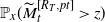 $\mathbb{P}_x(\widetilde{M}_t^{[R_T,pt]} \gt z)$
. In [Reference Yang and Zhu20, Lemma 4.3], let
$\mathbb{P}_x(\widetilde{M}_t^{[R_T,pt]} \gt z)$
. In [Reference Yang and Zhu20, Lemma 4.3], let $A=-z$
; then
$A=-z$
; then $I = \mathbb{P}_x(\widetilde{M}_t^{[pt,t]} \gt z)$
and
$I = \mathbb{P}_x(\widetilde{M}_t^{[pt,t]} \gt z)$
and $\mathit{II} = \mathbb{P}_x(\widetilde{M}_t^{[R_T,pt]} \gt z)$
. By the proof of [Reference Yang and Zhu20, Lemma 4.3], we have
$\mathit{II} = \mathbb{P}_x(\widetilde{M}_t^{[R_T,pt]} \gt z)$
. By the proof of [Reference Yang and Zhu20, Lemma 4.3], we have
 \begin{align*} I = \mathbb{P}_x\big(\widetilde{M}_t^{[pt,t]} \gt z\big) & \leq \frac{C}{p^{{3}/{2}}}\int_{pt}^{\infty}{\mathrm{e}}^{-({\rho}/{\sqrt{2}} - 1)^2r}\,\mathrm{d}r, \\ \mathit{II} = \mathbb{P}_x\big(\widetilde{M}_t^{[R_T,pt]} \gt z\big) & \leq C\Pi_x\bigg[\underline{\tau}_{0}^{\sqrt{2}-\rho} \mathbf{1}_{\big\{\underline{\tau}_{0}^{\sqrt{2}-\rho}\geq R_T\big\}}\bigg] \\ & = C\int_{R_T}^{\infty}\frac{rx}{\sqrt{2\pi r^3}\,}\exp\!\bigg\{{-}\frac{(x-(\sqrt{2}-\rho)r)^2}{2r}\bigg\}\, \mathrm{d}r, \end{align*}
where the positive constant C changes line by line and depends only on x, $\rho$
, and z. Here,
$\rho$
, and z. Here, $\{B_t, \Pi_x\}$
is a standard Brownian motion starting from x, and
$\{B_t, \Pi_x\}$
is a standard Brownian motion starting from x, and $\underline{\tau}_{0}^{\sqrt{2}-\rho} \,:\!=\, \inf\{s\geq 0\colon B_s \leq (\sqrt{2}-\rho)s\}$
.
$\underline{\tau}_{0}^{\sqrt{2}-\rho} \,:\!=\, \inf\{s\geq 0\colon B_s \leq (\sqrt{2}-\rho)s\}$
.
For any $\delta>0$
, by Markov’s inequality and Fubini’s theorem,
$\delta>0$
, by Markov’s inequality and Fubini’s theorem,
 \begin{align*} \mathbb{P}_x\bigg(\frac{1}{T}\int_{\varepsilon T}^T\mathbf{1}_{\big\{\widetilde{M}_t^{[pt,t]} \gt z\big\}}\,\mathrm{d}t \geq \delta\bigg) & \leq \frac{1}{\delta}\frac{1}{T}\int_{\varepsilon T}^T\mathbb{P}\big(\widetilde{M}_t^{[pt,t]} \gt z\big)\, \mathrm{d}t \\ & \leq \frac{C}{\delta Tp^{3/2}}\int_{\varepsilon T}^T\int_{pt}^{\infty}{\mathrm{e}}^{-({\rho}/{\sqrt{2}}-1)^2r}\,\mathrm{d}r\, \mathrm{d}t \\ & \leq \frac{C}{\delta Tp^{5/2}}{\mathrm{e}}^{-({\rho}/{\sqrt{2}}-1)^2p\varepsilon T}, \end{align*}
which is summable over $T\in\mathbb{N}$
. Therefore, by the Borel–Cantelli lemma,
$T\in\mathbb{N}$
. Therefore, by the Borel–Cantelli lemma,
 \begin{equation*} \mathbb{P}_x\bigg[\bigg\{\frac{1}{T}\int_{\varepsilon T}^T\mathbf{1}_{\big\{\widetilde{M}_t^{[pt,t]} \gt z\big\}}\,\mathrm{d}t \geq \delta\bigg\} \mbox{ infinitely often}\bigg] = 0. \end{equation*}
Hence,
 \begin{equation} \limsup_{T\uparrow\infty}\frac{1}{T}\int_{\varepsilon T}^T\mathbf{1}_{\big\{\widetilde{M}_t^{[pt,t]} \gt z\big\}}\,\mathrm{d}t = 0, \quad \mathbb{P}_x\mbox{-a.s.} \end{equation}
Using the same argument as above,
 \begin{align*} \mathbb{P}_x\bigg(\frac{1}{T}\int_{\varepsilon T}^T\mathbf{1}_{\big\{\widetilde{M}_t^{[R_T,pt]} \gt z\big\}}\,\mathrm{d}t \geq \delta\bigg) & \leq \frac{C}{\delta T}\int_{\varepsilon T}^T\int_{R_T}^{\infty}\frac{rx}{\sqrt{2\pi r^3}\,} \exp\!\bigg\{{-}\frac{(x-(\sqrt{2}-\rho)r)^2}{2r}\bigg\}\,\mathrm{d}r\,\mathrm{d}t \\ & \leq \frac{C}{\delta}\int_{R_T}^{\infty}\frac{x}{\sqrt{2\pi r}} \exp\!\bigg\{{-}\frac{(\sqrt{2}-\rho)^2}{2}r + (\sqrt{2}-\rho)x\bigg\}\,\mathrm{d}r, \end{align*}
which is summable in $T\in\mathbb{N}$
when
$T\in\mathbb{N}$
when $R_T/T^l\rightarrow\infty$
as
$R_T/T^l\rightarrow\infty$
as $T\rightarrow\infty$
for some
$T\rightarrow\infty$
for some $l>0$
. Therefore,
$l>0$
. Therefore,
 \begin{equation} \limsup_{T\uparrow\infty}\frac{1}{T}\int_{\varepsilon T}^T\mathbf{1}_{\big\{\widetilde{M}_t^{[R_T,pt]} \gt z\big\}}\,\mathrm{d}t = 0, \quad \mathbb{P}_x\mbox{-a.s.} \end{equation}
By (4.1), (4.2), and (4.3), we get (2.5). This completes the proof.
Appendix A. Proof of Claim A
Proof. The results in [Reference Arguin, Bovier and Kistler1] already imply this claim, and it can be directly derived with only minor modifications. According to [Reference Arguin, Bovier and Kistler1, (5.5), (5.54), (5.62), and (5.63)], (3.2) holds for any compact interval $\mathcal{D}$
. However, we require (3.2) to remain valid when the compact interval
$\mathcal{D}$
. However, we require (3.2) to remain valid when the compact interval $\mathcal{D}$
is replaced by
$\mathcal{D}$
is replaced by $[D,\infty)$
. With a slight modification, the proof given in [Reference Arguin, Bovier and Kistler1] continues to apply.
$[D,\infty)$
. With a slight modification, the proof given in [Reference Arguin, Bovier and Kistler1] continues to apply.
For any $x\in \mathbb{R} $
,
$x\in \mathbb{R} $
, $t>r>0$
, and interval
$t>r>0$
, and interval $\mathcal{A}$
, define
$\mathcal{A}$
, define $\mathrm{P}(x,t,r,\mathcal{A}) = \mathbb{P}_x[\text{there exists}$ $u\in N_t\colon X_u(t) - m_t\in\mathcal{A}$
but u is not localized during
$u\in N_t\colon X_u(t) - m_t\in\mathcal{A}$
but u is not localized during $(r,t-r)]$
. Let
$(r,t-r)]$
. Let $\mathcal{D}_b = [b,b+1]$
and
$\mathcal{D}_b = [b,b+1]$
and $\theta\in(0,\alpha)$
. We write
$\theta\in(0,\alpha)$
. We write $\lfloor s \rfloor$
for the largest integer less than or equal to s. The key proof strategy of this claim is to decompose
$\lfloor s \rfloor$
for the largest integer less than or equal to s. The key proof strategy of this claim is to decompose $[D,\infty)$
as
$[D,\infty)$
as $[D,\infty) \subset \big(\bigcup_{b=\lfloor D\rfloor}^{\lfloor r^{\theta}\rfloor}\mathcal{D}_b\big) \cup [r^{\theta},\infty)$
, and then apply the result from [Reference Arguin, Bovier and Kistler1] to
$[D,\infty) \subset \big(\bigcup_{b=\lfloor D\rfloor}^{\lfloor r^{\theta}\rfloor}\mathcal{D}_b\big) \cup [r^{\theta},\infty)$
, and then apply the result from [Reference Arguin, Bovier and Kistler1] to $\mathrm{P}(x,t,r,\mathcal{D}_b)$
. First, we will show that there exist
$\mathrm{P}(x,t,r,\mathcal{D}_b)$
. First, we will show that there exist $r_1,\delta_1>0$
depending on
$r_1,\delta_1>0$
depending on $\alpha$
,
$\alpha$
, $\beta$
, and D such that, for
$\beta$
, and D such that, for $r\geq r_1$
and
$r\geq r_1$
and $b\in[\lfloor D \rfloor,r^{\theta}]$
, the following holds:
$b\in[\lfloor D \rfloor,r^{\theta}]$
, the following holds:
 \begin{equation} \sup\nolimits_{t\geq 3r}\mathrm{P}(x,t,r,\mathcal{D}_b) \leq \exp\{-r^{\delta_1} \}. \end{equation}
To prove (A.1), we repeat the proof of [Reference Arguin, Bovier and Kistler1, Theorems 2.3 and 2.5, pp. 1668–74] when the compact set $\mathcal{D}$
is replaced by
$\mathcal{D}$
is replaced by $\mathcal{D}_b = [b,b+1]$
.
$\mathcal{D}_b = [b,b+1]$
.
When $\mathcal{D}_b = [b,b+1]$
, we have
$\mathcal{D}_b = [b,b+1]$
, we have $\overline{D} = b+1$
and
$\overline{D} = b+1$
and $\underline{D} = b$
in [Reference Arguin, Bovier and Kistler1, (5.20)]. Notice that for
$\underline{D} = b$
in [Reference Arguin, Bovier and Kistler1, (5.20)]. Notice that for $b\geq D$
, [Reference Arguin, Bovier and Kistler1, (5.25)] implies that
$b\geq D$
, [Reference Arguin, Bovier and Kistler1, (5.25)] implies that ${\mathrm{e}}^t\Pi[B_t\in m_t+\mathcal{D}_b] \leq \kappa t{\mathrm{e}}^{-\sqrt{2}D}$
. The upper bound of this probability does not depend on b. In [Reference Arguin, Bovier and Kistler1, line 5, p. 1670], we need to choose r large enough that
${\mathrm{e}}^t\Pi[B_t\in m_t+\mathcal{D}_b] \leq \kappa t{\mathrm{e}}^{-\sqrt{2}D}$
. The upper bound of this probability does not depend on b. In [Reference Arguin, Bovier and Kistler1, line 5, p. 1670], we need to choose r large enough that $\underline{F}\leq 0$
on
$\underline{F}\leq 0$
on $[r,t-r]$
, where
$[r,t-r]$
, where $\underline{F}$
is given by [Reference Arguin, Bovier and Kistler1, (5.32)]. For any
$\underline{F}$
is given by [Reference Arguin, Bovier and Kistler1, (5.32)]. For any $\delta,t>0$
, define
$\delta,t>0$
, define $f_{t,\delta}(s) = \min\{s^{\delta},(t-s)^{\delta}\}$
for
$f_{t,\delta}(s) = \min\{s^{\delta},(t-s)^{\delta}\}$
for $0\leq s \leq t$
. For
$0\leq s \leq t$
. For $b < r^{\theta} < r^{\alpha}$
and any
$b < r^{\theta} < r^{\alpha}$
and any $s\in [r,t-r]$
,
$s\in [r,t-r]$
,
 \begin{equation*} \underline{F}(s) = b\frac{t-s}{t} - f_{t,\alpha}(s) \leq b - r^{\alpha} \lt 0, \end{equation*}
which satisfies the condition. The remaining proof of [Reference Arguin, Bovier and Kistler1, Theorem 2.3] remains unchanged.
In the proof of [Reference Arguin, Bovier and Kistler1, Theorem 2.5], for sufficiently large r we have
 \begin{equation*} \mathrm{diam}(\mathcal{D}) = |\overline{D}| + |\underline{D}| \leq 2b+1 \leq 3r^{\theta}. \end{equation*}
Notice that $0<\theta<\alpha<\frac{1}{2}<\beta<1$
, and let
$0<\theta<\alpha<\frac{1}{2}<\beta<1$
, and let $0<a<1$
be such that
$0<a<1$
be such that $2a\beta-1>0$
. We can find
$2a\beta-1>0$
. We can find $\widetilde{r} = \widetilde{r}(\alpha,\beta,\theta,D,a)$
such that for
$\widetilde{r} = \widetilde{r}(\alpha,\beta,\theta,D,a)$
such that for $r\geq \widetilde{r}$
the following holds:
$r\geq \widetilde{r}$
the following holds: $3r^{\theta} - f_{t,\alpha}(s) \leq 0$
and
$3r^{\theta} - f_{t,\alpha}(s) \leq 0$
and $3r^{\theta} - f_{t,\beta}(s) \leq -f_{t,a\beta}(s)$
for all
$3r^{\theta} - f_{t,\beta}(s) \leq -f_{t,a\beta}(s)$
for all $r\leq s\leq t-r$
. Therefore, the proof of [Reference Arguin, Bovier and Kistler1, Theorem 2.5] is also valid and (A.1) holds for
$r\leq s\leq t-r$
. Therefore, the proof of [Reference Arguin, Bovier and Kistler1, Theorem 2.5] is also valid and (A.1) holds for $b\in [D,r^{\theta}]$
.
$b\in [D,r^{\theta}]$
.
By [Reference Arguin, Bovier and Kistler2, Corollary 10], for sufficiently large r and $t\geq 3r$
we have
$t\geq 3r$
we have
 \begin{equation} \mathrm{P}(x,t,r,[r^{\theta},\infty)) \leq \mathbb{P}_x[M_t \geq m_t + r^{\theta}] \leq Cr^{\theta}{\mathrm{e}}^{-\sqrt{2}r^{\theta}+1} \end{equation}
for some constant $C>0$
. Therefore, combining (A.1) with (A.2), we get that
$C>0$
. Therefore, combining (A.1) with (A.2), we get that
 \begin{align*} \sup\nolimits_{t\geq 3r}\mathrm{P}(x,t,r,[D,\infty)) & \leq \sum_{b = \lfloor D \rfloor}^{\lfloor r^{\theta}\rfloor}\mathrm{P}(x,t,r,\mathcal{D}_b) + \mathrm{P}(x,t,r,[r^{\theta},\infty)) \\ & \leq (|D|+r^{\theta}){\mathrm{e}}^{-r^{\delta_1}} + Cr^{\theta}{\mathrm{e}}^{-\sqrt{2}r^{\theta}+1}. \end{align*}
Choosing $\delta \lt \min\{\delta_1,\theta\}$
, there exists a sufficiently large
$\delta \lt \min\{\delta_1,\theta\}$
, there exists a sufficiently large $r_0$
such that (3.3) holds for
$r_0$
such that (3.3) holds for $r\geq r_0$
. This completes the proof.
$r\geq r_0$
. This completes the proof.
Acknowledgements
We thank Professor Xinxin Chen for many constructive suggestions, and, in particular, for providing the proof strategy of Claim A. We also thank the referee for very helpful comments on the first version of this paper.
Funding information
The research of this project is supported by the National Key R&D Program of China (No. 2020YFA0712900). The research of F. Yang is supported by China Postdoctoral Science Foundation (No. 2023TQ0033) and Postdoctoral Fellowship Program of CPSF (No. GZB20230068).
Competing interests
There were no competing interests to declare which arose during the preparation or publication process of this article.