


1. Introduction
Stellarators offer a promising path to realising controlled thermonuclear fusion as steady-state magnetic plasma confinement schemes (Boozer Reference Boozer2021). Their benefits arise from the freedom in the three-dimensional shaping of the magnetic field, away from the constraining requirement of axisymmetry (Wesson & Campbell Reference Wesson and Campbell2011), which is at the heart of the tokamak concept. However, this increase in the complexity of the magnetic field shaping and the loss of symmetry require careful tailoring, in particular, to prevent prompt collisionless losses of particles. The latter is commonly achieved through numerical optimisation, by seeking properties such as quasisymmetry (Boozer Reference Boozer1983; Nührenberg & Zille Reference Nührenberg and Zille1988; Rodriguez et al. Reference Rodriguez, Helander and Bhattacharjee2020) or, more generally, omnigeneity (Hall & McNamara Reference Hall and McNamara1975; Bernardin, Moses & Tataronis Reference Bernardin, Moses and Tataronis1986; Cary & Shasharina Reference Cary and Shasharina1997; Landreman & Catto Reference Landreman and Catto2012; Dudt et al. Reference Dudt, Goodman, Conlin, Panici and Kolemen2024), alongside other additional requirements (aspect ratio, magnetohydrodynamic (MHD) stability, coil complexity, etc.). The problem of finding stellarator designs is therefore a multi-objective optimisation problem in a high-dimensional optimisation space, with multiple minima and in which evaluation of each point (i.e. computation of three-dimensional isotropic pressure, ideal magnetohydrostatic (MHS) equilibrium) is time consuming. While this method has been successfully applied to produce attractive stellarator designs (Nührenberg & Zille Reference Nührenberg and Zille1988; Anderson et al. Reference Anderson, Almagri, Anderson, Matthews, Talmadge and Shohet1995; Zarnstorff et al. Reference Zarnstorff2001; Ku & Boozer Reference Ku and Boozer2010; Landreman & Paul Reference Landreman and Paul2022), it is a daunting (if not impossible) task to conduct an exhaustive solution space scan (Landreman Reference Landreman2019; Giuliani, Rodríguez & Spivak Reference Giuliani, Rodríguez and Spivak2024).
To alleviate some of this burden, and gain additional insight into what that vast space of stellarators may look like, analytic insight can be gained through the near-axis expansion (NAE) (Mercier Reference Mercier1964; Solov’ev & Shafranov Reference Solov’ev and Shafranov1970; Lortz & Nührenberg Reference Lortz and Nührenberg1976; Garren & Boozer Reference Garren and Boozer1991b ; Landreman & Sengupta Reference Landreman and Sengupta2019; Rodríguez et al. Reference Rodríguez, Plunk and Jorge2025). This is an asymptotic description of the field in the distance from its centre (the magnetic axis), which constitutes a simple consistent model of stellarator fields. This approach has the benefit of reducing the MHS equilibrium problem, alongside omnigeneity conditions, to a reduced set of parameters and functions (Garren & Boozer Reference Garren and Boozer1991a ; Landreman, Sengupta & Plunk Reference Landreman, Sengupta and Plunk2019; Plunk et al. Reference Plunk, Landreman and Helander2019; Rodríguez et al. Reference Rodríguez, Plunk and Jorge2025) related through algebraic and ordinary differential equations that may be numerically solved orders of magnitude faster than their global counterparts (Landreman et al. Reference Landreman, Sengupta and Plunk2019; Panici et al. Reference Panici, Conlin, Dudt, Unalmis and Kolemen2023). This has enabled more exhaustive exploration of the space of stellarators (Landreman Reference Landreman2022a; Rodriguez, Sengupta & Bhattacharjee Reference Rodriguez, Sengupta and Bhattacharjee2023; Giuliani et al. Reference Giuliani, Rodríguez and Spivak2024). Besides this practical difference, NAE theory has also been shown to be a natural lens through which to understand the space of optimised stellarators, particularly quasisymmetric ones (Landreman & Sengupta Reference Landreman and Sengupta2019; Rodríguez et al. Reference Rodríguez, Sengupta and Bhattacharjee2022b , Reference Rodriguez, Sengupta and Bhattacharjee2023).
The NAE theory offers a sensible path to searching for candidate stellarator configurations with desirable confinement properties. However, the theory is still fundamentally an asymptotic theory: the solutions it finds are only valid in some volume near the axis. The further away, the less reliable the description becomes, and thus global MHS solutions are still required to fully characterise the stellarator equilibrium. It is natural, however, to employ the near-axis construction as a starting point for higher-fidelity field construction, and thus it is necessary to devise a way of connecting global equilibrium solutions to the near-axis ones. The current standard method evaluates the NAE field at a finite distance from the axis, constructs the corresponding flux surface and uses it as an input to conventional nested flux surface global (fixed-boundary) MHS codes (Hirshman & Whitson Reference Hirshman and Whitson1983; Dudt et al. Reference Dudt, Conlin, Panici, Unalmis, Kim and Kolemen2022; Hindenlang, Plunk & Maj Reference Hindenlang, Plunk and Maj2025). Although this procedure has proved effective, there is a blatant fault to it: the NAE is being used to inform the global solution at a point where it is least valid (far from the axis). The result is that many of the features curated into the NAE fields are lost when building the equilibria, especially at lower aspect ratios.
This paper introduces a new method of finding global three-dimensional (3-D) MHS equilibrium solutions, in the equilibrium solver DESC, which are intimately connected to NAE theory. We do so by constraining the global solution’s near-axis behaviour directly, using information from the NAE where it is most valid. This way of connecting the asymptotic behaviour to global equilibrium will preserve any near-axis property studied, understood or optimised for within the near-axis framework. While we do so, we leave freedom to the global MHS solver to mould the solution far from the axis, where the NAE loses accuracy. This results in global MHS solutions with near-axis behaviour consistent with the NAE, and far-from-axis behaviour consistent with solving the global MHS equilibrium equations.
The paper is organised as follows. Section 2 presents both formulations of the equilibrium problem as they are done in the NAE and DESC, in order to link them to each other. Section 3 will then use this connection to derive, order by order up to second order in the distance from the axis, the geometric constraints on the DESC equilibrium which enforce the NAE behaviour. Section 4.1 then presents some examples of the constrained equilibria, which are also used to verify the correct enforcement of the NAE behaviour in the global equilibrium.
2. Connecting the near-axis description
The goal of the paper is simple: we aim to construct global equilibria given some prescribed near-axis behaviour. To do so, we first need to understand how to deal with the equilibrium problem.
2.1. The equilibrium problem
We define an equilibrium solution as a magnetic field with nested flux surfaces that satisfies the MHS equilibrium equation
 $\boldsymbol{j}\times \boldsymbol{B}=\boldsymbol{\nabla }p$
, where
$\boldsymbol{j}\times \boldsymbol{B}=\boldsymbol{\nabla }p$
, where
 $\boldsymbol{j}=\mu _0^{-1}\boldsymbol{\nabla }\times \boldsymbol{B}$
is the plasma current density,
$\boldsymbol{j}=\mu _0^{-1}\boldsymbol{\nabla }\times \boldsymbol{B}$
is the plasma current density,
 $p$
is the plasma pressure, and
$p$
is the plasma pressure, and
 $\mu_0$
is the vacuum permeability. The magnetic field must, of course, be a solenoidal vector field,
$\mu_0$
is the vacuum permeability. The magnetic field must, of course, be a solenoidal vector field,
 $\boldsymbol{\nabla }\boldsymbol{\cdot }\boldsymbol{B}=0$
, and we define a toroidal magnetic flux
$\boldsymbol{\nabla }\boldsymbol{\cdot }\boldsymbol{B}=0$
, and we define a toroidal magnetic flux
 $2\pi \psi$
whose level sets define nested flux surfaces satisfying
$2\pi \psi$
whose level sets define nested flux surfaces satisfying
 $\boldsymbol{B}\boldsymbol{\cdot }\boldsymbol{\nabla }\psi =0$
. Both the global equilibrium solver and the near-axis description attempt the construction of equilibrium fields of this form.
$\boldsymbol{B}\boldsymbol{\cdot }\boldsymbol{\nabla }\psi =0$
. Both the global equilibrium solver and the near-axis description attempt the construction of equilibrium fields of this form.
Within this set of equations, we confer on the latter two a more prominent role. That is, we prioritise the magnetic field being solenoidal and having nested flux surfaces, which we impose on the field in an exact form. This is done by adopting the inverse-coordinate form of the problem (Bauer, Betancourt & Garabedian Reference Bauer, Betancourt and Garabedian1978; Hirshman & Whitson Reference Hirshman and Whitson1983). Instead of describing the magnetic field
 $\boldsymbol{B}$
explicitly as a function of space, we instead focus on describing the magnetic flux surfaces on which the field lives, as well as the form in which field lines wrap over them.
$\boldsymbol{B}$
explicitly as a function of space, we instead focus on describing the magnetic flux surfaces on which the field lives, as well as the form in which field lines wrap over them.
To construct such a description, we start by writing the magnetic field in its Clebsch form (D’haeseleer et al. Reference D’haeseleer, Hitchon, Callen and Shohet2012)
 \begin{equation} \boldsymbol{B}=\boldsymbol{\nabla }\psi \times (\boldsymbol{\nabla }\vartheta -\iota \boldsymbol{\nabla }\varphi ), \end{equation}
where
 $\vartheta$
and
$\vartheta$
and
 $\varphi$
are poloidal and toroidal angles (in straight field line coordinates with non-vanishing Jacobian), and
$\varphi$
are poloidal and toroidal angles (in straight field line coordinates with non-vanishing Jacobian), and
 $\iota$
(a function of
$\iota$
(a function of
 $\psi$
) is the rotational transform. A field written in this form satisfies both field requirements exactly. Defining a position vector
$\psi$
) is the rotational transform. A field written in this form satisfies both field requirements exactly. Defining a position vector
 $\boldsymbol{x}=\boldsymbol{x}(\psi ,\vartheta ,\varphi )$
, and taking that set of straight field line coordinates as our set of independent coordinates, the magnetic field may then be expressed as
$\boldsymbol{x}=\boldsymbol{x}(\psi ,\vartheta ,\varphi )$
, and taking that set of straight field line coordinates as our set of independent coordinates, the magnetic field may then be expressed as
 \begin{equation} \boldsymbol{B}=\mathcal{J}_\vartheta ^{-1}\left (\frac {\partial \boldsymbol{x}}{\partial \varphi }+\iota \frac {\partial \boldsymbol{x}}{\partial \vartheta }\right )\!, \end{equation}
where
 $\mathcal{J}_\vartheta =\partial _\psi \boldsymbol{x}\times \partial _\vartheta \boldsymbol{x}\boldsymbol{\cdot }\partial _\varphi \boldsymbol{x}$
is the Jacobian of the straight field line coordinate system. Full knowledge of flux surfaces in straight field line coordinates (i.e.
$\mathcal{J}_\vartheta =\partial _\psi \boldsymbol{x}\times \partial _\vartheta \boldsymbol{x}\boldsymbol{\cdot }\partial _\varphi \boldsymbol{x}$
is the Jacobian of the straight field line coordinate system. Full knowledge of flux surfaces in straight field line coordinates (i.e.
 $\boldsymbol{x}$
), along with the rotational transform, uniquely defines the magnetic field. Alternatively, one could provide information about the average toroidal current rather than the rotational transform (see Appendix A).
$\boldsymbol{x}$
), along with the rotational transform, uniquely defines the magnetic field. Alternatively, one could provide information about the average toroidal current rather than the rotational transform (see Appendix A).
The central task is then to find a function
 $\boldsymbol{x}(\psi ,\vartheta ,\varphi )$
, which we may represent in a multitude of ways. The NAE, in its inverse-coordinate form pioneered by Garren & Boozer (Reference Garren and Boozer1991c
), takes as a reference of this
$\boldsymbol{x}(\psi ,\vartheta ,\varphi )$
, which we may represent in a multitude of ways. The NAE, in its inverse-coordinate form pioneered by Garren & Boozer (Reference Garren and Boozer1991c
), takes as a reference of this
 $\boldsymbol{x}$
the magnetic axis. This is a natural choice given that the NAE is concerned with providing a consistent asymptotic description of the field near the magnetic axis (i.e.
$\boldsymbol{x}$
the magnetic axis. This is a natural choice given that the NAE is concerned with providing a consistent asymptotic description of the field near the magnetic axis (i.e.
 $\psi =0$
). Explicitly,
$\psi =0$
). Explicitly,
 \begin{equation} \boldsymbol{x}(\psi ,\vartheta ,\varphi )=\boldsymbol{r}_0+X(\psi ,\vartheta ,\varphi )\hat {\boldsymbol \kappa }+Y(\psi ,\vartheta ,\varphi )\hat {\boldsymbol \tau }+Z(\psi ,\vartheta ,\varphi )\hat {\boldsymbol{t}}, \end{equation}
where
 $\boldsymbol{r}_0$
describes the magnetic axis, and the vector triad
$\boldsymbol{r}_0$
describes the magnetic axis, and the vector triad
 $\{\hat {\boldsymbol \kappa },\hat {\boldsymbol \tau },\hat {\boldsymbol{t}}\}$
corresponds to the Frenet–Serret basis (Frenet Reference Frenet1852; Animov Reference Animov2001) (namely, the normal, binormal and tangent vectors defined with respect to the magnetic axis). Here, we specialise to regular magnetic axes with no, or only few, isolated flattening points (i.e. vanishing curvature points) in which such a frame (or its signed version (Carroll, Köse & Sterling Reference Carroll, Köse and Sterling2013; Plunk et al. Reference Plunk, Landreman and Helander2019; Camacho Mata & Plunk Reference Camacho Mata and Plunk2023; Rodríguez et al. Reference Rodríguez, Plunk and Jorge2025)) exists. This is enough to describe the asymptotic behaviour of all optimised configurations; namely, quasisymmetric and quasi-isodynamic ones (Gori, Lotz & Nührenberg Reference Gori, Lotz and Nührenberg1997; Plunk et al. Reference Plunk, Landreman and Helander2019). In the NAE, then, finding a magnetic field corresponds to finding an asymptotic form of the functions
$\{\hat {\boldsymbol \kappa },\hat {\boldsymbol \tau },\hat {\boldsymbol{t}}\}$
corresponds to the Frenet–Serret basis (Frenet Reference Frenet1852; Animov Reference Animov2001) (namely, the normal, binormal and tangent vectors defined with respect to the magnetic axis). Here, we specialise to regular magnetic axes with no, or only few, isolated flattening points (i.e. vanishing curvature points) in which such a frame (or its signed version (Carroll, Köse & Sterling Reference Carroll, Köse and Sterling2013; Plunk et al. Reference Plunk, Landreman and Helander2019; Camacho Mata & Plunk Reference Camacho Mata and Plunk2023; Rodríguez et al. Reference Rodríguez, Plunk and Jorge2025)) exists. This is enough to describe the asymptotic behaviour of all optimised configurations; namely, quasisymmetric and quasi-isodynamic ones (Gori, Lotz & Nührenberg Reference Gori, Lotz and Nührenberg1997; Plunk et al. Reference Plunk, Landreman and Helander2019). In the NAE, then, finding a magnetic field corresponds to finding an asymptotic form of the functions
 $X,\,Y$
and
$X,\,Y$
and
 $Z$
, which describe the shape of flux surfaces, alongside the rotational transform and the axis shape. This description is performed in a special class of straight field line coordinates, Boozer coordinates
$Z$
, which describe the shape of flux surfaces, alongside the rotational transform and the axis shape. This description is performed in a special class of straight field line coordinates, Boozer coordinates
 $\{\psi ,\vartheta _{B},\varphi _{B}\}$
, which eases the treatment of optimised stellarators due to the simple involvement of
$\{\psi ,\vartheta _{B},\varphi _{B}\}$
, which eases the treatment of optimised stellarators due to the simple involvement of
 $|\boldsymbol{B}|$
(Boozer Reference Boozer1981), which imposes additional constraints in the construction.
$|\boldsymbol{B}|$
(Boozer Reference Boozer1981), which imposes additional constraints in the construction.
In the case of the global equilibrium description, the numerical solver DESC, which we shall focus on, describes flux surfaces not with respect to the axis (unlike new developments (Hindenlang et al. Reference Hindenlang, Plunk and Maj2025)), but in cylindrical coordinates so that
 \begin{equation} \boldsymbol{x}_{\mathrm{DESC}}=R \hat {\boldsymbol{R}} + Z \hat {\boldsymbol{Z}}. \end{equation}
It is then the task of the solver to find the appropriate
 $R$
and
$R$
and
 $Z$
functions as a function of
$Z$
functions as a function of
 $\{\psi ,\,\vartheta ,\,\varphi \}$
. Given that the description is in cylindrical coordinates, the toroidal angle is naturally chosen to be the cylindrical one,
$\{\psi ,\,\vartheta ,\,\varphi \}$
. Given that the description is in cylindrical coordinates, the toroidal angle is naturally chosen to be the cylindrical one,
 $\phi$
.Footnote
1
Because we insist on this specific form of the toroidal angle, it requires a very particular choice of the poloidal angle
$\phi$
.Footnote
1
Because we insist on this specific form of the toroidal angle, it requires a very particular choice of the poloidal angle
 $\vartheta$
in order to guarantee the coordinate system to be a straight field line coordinate system. This coordinate system is known as PEST coordinates
$\vartheta$
in order to guarantee the coordinate system to be a straight field line coordinate system. This coordinate system is known as PEST coordinates
 $\{\psi ,\vartheta _{\mathrm{PEST}},\phi \}$
. However, the global solver does not know at the starting point what
$\{\psi ,\vartheta _{\mathrm{PEST}},\phi \}$
. However, the global solver does not know at the starting point what
 $\vartheta _{\mathrm{PEST}}$
is, as this depends on the final magnetic field solution. Hence, in practice, the solver must introduce a stream function
$\vartheta _{\mathrm{PEST}}$
is, as this depends on the final magnetic field solution. Hence, in practice, the solver must introduce a stream function
 $\lambda$
such that
$\lambda$
such that
 $\vartheta _{\mathrm{PEST}}=\theta +\lambda$
, where
$\vartheta _{\mathrm{PEST}}=\theta +\lambda$
, where
 $\theta$
can be any arbitrary poloidal angle used by the equilibrium solver. In that case, the magnetic field, as in (2.2) is written as
$\theta$
can be any arbitrary poloidal angle used by the equilibrium solver. In that case, the magnetic field, as in (2.2) is written as
 \begin{equation} \boldsymbol{B}=\mathcal{J}_\theta ^{-1}\left [(1+\partial _\theta \lambda )\frac {\partial \boldsymbol{x}}{\partial \phi }+(\iota -\partial _\phi \lambda )\frac {\partial \boldsymbol{x}}{\partial \theta }\right ]\!. \end{equation}
Where now the Jacobian is of the computational coordinates
 $\mathcal{J}_\theta =\partial _\psi \boldsymbol{x}\times \partial _\theta \boldsymbol{x}\boldsymbol{\cdot }\partial _\varphi \boldsymbol{x}\!$
. In the case of the global solver then, a magnetic field is uniquely described by finding functions
$\mathcal{J}_\theta =\partial _\psi \boldsymbol{x}\times \partial _\theta \boldsymbol{x}\boldsymbol{\cdot }\partial _\varphi \boldsymbol{x}\!$
. In the case of the global solver then, a magnetic field is uniquely described by finding functions
 $R,\,Z$
and
$R,\,Z$
and
 $\lambda$
as a function of
$\lambda$
as a function of
 $\{\psi ,\,\theta ,\,\phi \}$
.
$\{\psi ,\,\theta ,\,\phi \}$
.
So far, we have only represented a magnetic field but have not yet solved the equilibrium. We must still find a consistent set of flux surfaces
 $\boldsymbol{x}$
(described in appropriate coordinates), such that the resulting magnetic field is in equilibrium. We must deform flux surfaces until the field comes to equilibrium; i.e. it minimises the force residual
$\boldsymbol{x}$
(described in appropriate coordinates), such that the resulting magnetic field is in equilibrium. We must deform flux surfaces until the field comes to equilibrium; i.e. it minimises the force residual
 $\boldsymbol{F}=\boldsymbol{j}\times \boldsymbol{B}-\boldsymbol{\nabla }p$
for a prescribed function
$\boldsymbol{F}=\boldsymbol{j}\times \boldsymbol{B}-\boldsymbol{\nabla }p$
for a prescribed function
 $p(\psi )$
. In the context of the NAE, the consistent construction of flux surfaces and Boozer coordinates can be carried out systematically by setting
$p(\psi )$
. In the context of the NAE, the consistent construction of flux surfaces and Boozer coordinates can be carried out systematically by setting
 $\boldsymbol{F} = \boldsymbol{0}$
order by order, and detailed descriptions of how to do this may be found in Landreman & Sengupta (Reference Landreman and Sengupta2019) and Rodríguez et al. (Reference Rodríguez, Plunk and Jorge2025). We content ourselves with knowing that, at the end of the day, we will be able to have an asymptotic form of a
$\boldsymbol{F} = \boldsymbol{0}$
order by order, and detailed descriptions of how to do this may be found in Landreman & Sengupta (Reference Landreman and Sengupta2019) and Rodríguez et al. (Reference Rodríguez, Plunk and Jorge2025). We content ourselves with knowing that, at the end of the day, we will be able to have an asymptotic form of a
 $X,Y,Z$
rotational transform and the axis shape.
$X,Y,Z$
rotational transform and the axis shape.
The equilibrium solver DESC seeks equilibria by numerically and iteratively minimising the force residual
 $\boldsymbol{F}$
directly. Note that this is not the only existing practical approach, with the important case of the VMEC code approaching the problem by minimising energy (Hirshman & Whitson Reference Hirshman and Whitson1983). To be more explicit about the force residual, consider first the covariant form of the magnetic field
$\boldsymbol{F}$
directly. Note that this is not the only existing practical approach, with the important case of the VMEC code approaching the problem by minimising energy (Hirshman & Whitson Reference Hirshman and Whitson1983). To be more explicit about the force residual, consider first the covariant form of the magnetic field
 \begin{equation} \boldsymbol{B}=B_\theta \boldsymbol{\nabla }\theta +B_\phi \boldsymbol{\nabla }\phi +B_\psi \boldsymbol{\nabla }\psi . \end{equation}
There might appear to be new information in the problem, but all of the covariant components in (2.6) can be directly computed from the geometry by simply leveraging the dual relations (D’haeseleer et al. Reference D’haeseleer, Hitchon, Callen and Shohet2012, (2.3.12)–(2.3.13))
 $\boldsymbol{\nabla }q_i=\epsilon _{ijk}\partial _{q_j}\boldsymbol{x}\times \partial _{q_k}\boldsymbol{x}$
and (2.5a
). With this, the force residual is (see Panici et al. (Reference Panici, Conlin, Dudt, Unalmis and Kolemen2023) as well)
$\boldsymbol{\nabla }q_i=\epsilon _{ijk}\partial _{q_j}\boldsymbol{x}\times \partial _{q_k}\boldsymbol{x}$
and (2.5a
). With this, the force residual is (see Panici et al. (Reference Panici, Conlin, Dudt, Unalmis and Kolemen2023) as well)
 \begin{align} \boldsymbol{F}&=\left [\mathcal{J}_\theta ^{-1}\mu _0^{-1}(\partial _\phi B_\psi -\partial _\psi B_\phi )(1+\partial _\theta \lambda )-\mathcal{J}_\theta ^{-1}\mu _0^{-1}(\iota -\partial _\phi \lambda )(\partial _\psi B_\theta -\partial _\theta B_\psi )-p'\right ]\boldsymbol{\nabla }\psi \nonumber \\& \quad -\mathcal{J}_\theta ^{-1}\mu _0^{-1}(\partial _\theta B_\phi -\partial _\phi B_\theta )((1+\partial _\theta \lambda )\boldsymbol{\nabla }\theta -(\iota -\partial _\phi \lambda )\boldsymbol{\nabla }\phi ). \end{align}
The
 $\boldsymbol{\nabla }\psi$
component can be interpreted as the radial force balance equation, with the helical component representing
$\boldsymbol{\nabla }\psi$
component can be interpreted as the radial force balance equation, with the helical component representing
 $\boldsymbol{j}\boldsymbol{\cdot }\boldsymbol{\nabla }\psi$
. Thus, the global solver is set to find
$\boldsymbol{j}\boldsymbol{\cdot }\boldsymbol{\nabla }\psi$
. Thus, the global solver is set to find
 $\{R,\,Z,\,\lambda \}$
as a function of
$\{R,\,Z,\,\lambda \}$
as a function of
 $\{\psi ,\theta ,\phi \}$
that make (2.7) vanish.
$\{\psi ,\theta ,\phi \}$
that make (2.7) vanish.
The near-axis and global treatments of the problem thus have a key difference not only in the coordinate representation used, but also in their treatment of boundary conditions. One must provide certain inputs to the equilibrium problem to describe different equilibria. In the NAE case, this prescription occurs outwards; that is, one must provide the shape of the axis, and then, order by order, some features of the flux surfaces away from it. Which features must be provided depends on the type of stellarator under consideration, and the order of the expansion of interest (see Landreman & Sengupta Reference Landreman and Sengupta2019; Rodríguez et al. Reference Rodríguez, Plunk and Jorge2025). The global solution fundamentally attempts the opposite: one specifies the shape of the boundary, and the solution is constructed inwards (what is known as a fixed-boundary solution). This is most straightforwardly understood by imagining a vacuum field in the form of Laplace’s equation. From this difference it should be clear that there is not a one-to-one correspondence between the two approaches. A finite truncated near-axis construction does not, in principle, uniquely describe a global field solution, but rather simply constrains its core behaviour. We are now in a position to connect both.
2.2. Near-axis expansion in DESC
In the NAE we learned that the description of flux surfaces
 $\boldsymbol{x}(\psi ,\vartheta _B,\varphi _B)$
is given by
$\boldsymbol{x}(\psi ,\vartheta _B,\varphi _B)$
is given by
 $\{X,Y,Z\}$
, (2.3). The forms of
$\{X,Y,Z\}$
, (2.3). The forms of
 $\{X,Y,Z\}$
are particularly simple, as may be directly appreciated by considering their Taylor–Fourier expansion (Garren & Boozer Reference Garren and Boozer1991c
; Landreman & Sengupta Reference Landreman and Sengupta2019)
$\{X,Y,Z\}$
are particularly simple, as may be directly appreciated by considering their Taylor–Fourier expansion (Garren & Boozer Reference Garren and Boozer1991c
; Landreman & Sengupta Reference Landreman and Sengupta2019)
 \begin{equation} f(\psi ,\theta _{B},\varphi _{B})=\sum _{l=0}^\infty r^l\sum _{m=0}^l{}^{\prime }\left (f_{lm}^C(\varphi _{B})\cos m\vartheta _{B}+f_{lm}^S(\varphi _B)\sin m\vartheta _{B}\right )\!, \end{equation}
where
 $r=\sqrt {2\psi /\bar {B}}$
is a pseudo-radial coordinate,
$r=\sqrt {2\psi /\bar {B}}$
is a pseudo-radial coordinate,
 $\bar {B}$
is a representative normalisation value of the magnetic field and the sum
$\bar {B}$
is a representative normalisation value of the magnetic field and the sum
 $\sum '$
denotes sum over even or odd orders depending on the parity of
$\sum '$
denotes sum over even or odd orders depending on the parity of
 $l$
. Because the poloidal dependence grows in a controlled manner linked to the powers of
$l$
. Because the poloidal dependence grows in a controlled manner linked to the powers of
 $r$
, the flux surfaces gain complexity order by order; they start by being elliptical, then acquire triangularity, and so on.
$r$
, the flux surfaces gain complexity order by order; they start by being elliptical, then acquire triangularity, and so on.
To impose this asymptotic form of the field on the global equilibrium solver, we must be able to relate this asymptotic description to the representation in DESC, and constrain the latter according to the former. The structure in (2.8) is a consequence of maintaining the field description singularity free close to the magnetic axis (
 $\psi =0$
) (Kuo-Petravic & Boozer Reference Kuo-Petravic and Boozer1987; Garren & Boozer Reference Garren and Boozer1991b
; Landreman & Sengupta Reference Landreman and Sengupta2018). This requirement was indeed observed in the implementation of DESC, where the global solver employs a Zernike basis to represent
$\psi =0$
) (Kuo-Petravic & Boozer Reference Kuo-Petravic and Boozer1987; Garren & Boozer Reference Garren and Boozer1991b
; Landreman & Sengupta Reference Landreman and Sengupta2018). This requirement was indeed observed in the implementation of DESC, where the global solver employs a Zernike basis to represent
 $\{R,Z,\lambda \}$
, crucially coupling the powers of DESC’s chosen pseudo-radial coordinate
$\{R,Z,\lambda \}$
, crucially coupling the powers of DESC’s chosen pseudo-radial coordinate
 $\rho =\sqrt {\psi /\psi _{\mathrm{edge}}}$
to the poloidal modes
$\rho =\sqrt {\psi /\psi _{\mathrm{edge}}}$
to the poloidal modes
 $\theta$
. This makes the treatment in DESC close to the form used in the near-axis description.
$\theta$
. This makes the treatment in DESC close to the form used in the near-axis description.
To make that connection, however, we must consider the differences carefully. One is the use of different re-scaled pseudo-radial coordinates; we may relate
 $\rho$
to the NAE
$\rho$
to the NAE
 $r$
by
$r$
by
 $\rho =r\sqrt {\bar {B}/2\psi _{\mathrm{edge}}}$
. The second point of difference is the use of a different poloidal angle. While the near-axis description uses the poloidal Boozer angle,
$\rho =r\sqrt {\bar {B}/2\psi _{\mathrm{edge}}}$
. The second point of difference is the use of a different poloidal angle. While the near-axis description uses the poloidal Boozer angle,
 $\vartheta _{B}$
, the global equilibrium is described in a general poloidal angle
$\vartheta _{B}$
, the global equilibrium is described in a general poloidal angle
 $\theta$
. The simplest comparison between the two descriptions is then made when
$\theta$
. The simplest comparison between the two descriptions is then made when
 $\theta$
is forced to match the Boozer angle, at least to leading order near the axis. When imposing the near-axis constraints on
$\theta$
is forced to match the Boozer angle, at least to leading order near the axis. When imposing the near-axis constraints on
 $\theta$
as if it were Boozer coordinates, the solver is forced to use a very particular form of
$\theta$
as if it were Boozer coordinates, the solver is forced to use a very particular form of
 $\lambda$
, and thus can be overly constraining. Defining
$\lambda$
, and thus can be overly constraining. Defining
 $\nu =\varphi _{B}-\phi$
as the function that maps the Boozer toroidal angle to the cylindrical one, our choice of
$\nu =\varphi _{B}-\phi$
as the function that maps the Boozer toroidal angle to the cylindrical one, our choice of
 $\theta$
dictates that
$\theta$
dictates that
 \begin{gather} \lambda =-\iota \nu . \end{gather}
This simplest choice of poloidal angle could be modified to accommodate a more general and efficient
 $\theta$
. Details about how this would be incorporated are shown in Appendix B, but we shall nevertheless consider the simplest scenario in the main body of the paper, which should suffice as a proof of principle.
$\theta$
. Details about how this would be incorporated are shown in Appendix B, but we shall nevertheless consider the simplest scenario in the main body of the paper, which should suffice as a proof of principle.
With the coordinates in place, what remains from the comparison is the different radial–poloidal structure of the NAE expansion and the Zernike basis. In the equilibrium solver a generic function is written as (ignoring the toroidal coordinate for now)
 \begin{equation} f(\rho ,\theta )=\sum _{l=0}^\infty \sum _{m=-l}^l{}^{\prime }f_{lm}\mathcal{Z}_l^m(\rho ,\theta ), \end{equation}
where the
 $\sum ^{\prime }$
again denotes a sum over the same parity as
$\sum ^{\prime }$
again denotes a sum over the same parity as
 $l$
, and the Zernike polynomials are
$l$
, and the Zernike polynomials are
 \begin{equation} \mathcal{Z}_l^m(\rho ,\theta )=\mathcal{R}_l^{|m|}\begin{cases} \cos (m\theta ) & m\geqslant 0, \\ \sin (|m|\theta ) & m\lt 0, \end{cases} \end{equation}
where the radial parts are the shifted Jacobi polynomials, given as
 \begin{equation} \mathcal{R}_l^{|m|}=\sum _{k=0}^{(l-|m|)/2}\frac {(-1)^k(l-k)!}{k!\left ((({l+m})/{2})-k\right )!\left ((({l-m})/{2})-k\right )!}\rho ^{l-2k}. \end{equation}
The coefficients
 $\{f_{lm}\}$
for
$\{f_{lm}\}$
for
 $\{R,Z,\lambda \}$
are the set which DESC solves for in order to construct the equilibrium field. To make a one-to-one connection to the NAE, (2.8), we need to unravel this sum and pick the different powers of
$\{R,Z,\lambda \}$
are the set which DESC solves for in order to construct the equilibrium field. To make a one-to-one connection to the NAE, (2.8), we need to unravel this sum and pick the different powers of
 $\rho$
. Generally, a function
$\rho$
. Generally, a function
 $f$
defined by
$f$
defined by
 $f_{lm}$
coefficients can be written in terms of the equivalent near-axis coefficients as
$f_{lm}$
coefficients can be written in terms of the equivalent near-axis coefficients as
 \begin{equation} f_{l|m|}^{C/S}=\left (\frac {\rho }{r}\right )^l\times \begin{cases} \begin{aligned} &(-1)^{l/2}\sum _{k=l/2}^\infty \Bigg [ (-1)^k\binom {k+l/2}{l}\\&\hspace {1in} \times \binom {l}{(l-|m|)/2}f_{2k,m}\Bigg ]\quad |m| \mathrm{\,is\,even} ,\\ &(-1)^{(l+1)/2}\sum _{k=(l+1)/2}^\infty \Bigg [(-1)^k\binom {k+(l-1)/2}{l}\\&\hspace {1in}\times \binom {l}{(l-|m|)/2}f_{2k-1,m}\Bigg ] \quad |m| \mathrm{\,is\,odd}, \\ \end{aligned} \end{cases} \end{equation}
and the sign of
 $m$
has been taken to represent, as is the case in the DESC notation, the sine or cosine terms
$m$
has been taken to represent, as is the case in the DESC notation, the sine or cosine terms
 $S/C$
(negative and positive respectively).Footnote
2
The above only holds for
$S/C$
(negative and positive respectively).Footnote
2
The above only holds for
 $l\geqslant |m|$
, and
$l\geqslant |m|$
, and
 $m$
sharing the same parity as
$m$
sharing the same parity as
 $l$
. Otherwise, the contribution will be zero. Note how, for large
$l$
. Otherwise, the contribution will be zero. Note how, for large
 $k$
at constant
$k$
at constant
 $l$
and
$l$
and
 $m$
, the factor in front of the Zernike components goes like
$m$
, the factor in front of the Zernike components goes like
 $\sim k^l$
. This shows the exponential contribution from the higher-order Zernike modes, which must therefore be conveniently truncated. See details on the derivation in Appendix C. Thus, imposing the near-axis behaviour constitutes imposing constraints on linear combinations of the DESC degrees of freedom.
$\sim k^l$
. This shows the exponential contribution from the higher-order Zernike modes, which must therefore be conveniently truncated. See details on the derivation in Appendix C. Thus, imposing the near-axis behaviour constitutes imposing constraints on linear combinations of the DESC degrees of freedom.
As a final remark, we note that what have been referred to as coefficients
 $f_{lm}$
so far are generally functions of
$f_{lm}$
so far are generally functions of
 $\phi$
. In the pseudo-spectral representation of DESC, we may then treat the toroidal dependence with a Fourier series in
$\phi$
. In the pseudo-spectral representation of DESC, we may then treat the toroidal dependence with a Fourier series in
 $\phi$
, with the
$\phi$
, with the
 $n$
Fourier components corresponding to
$n$
Fourier components corresponding to
 $f_{lmn}$
, with
$f_{lmn}$
, with
 $n\geqslant 0$
representing cosines, and
$n\geqslant 0$
representing cosines, and
 $n\lt 0$
sines.
$n\lt 0$
sines.
3. Constraining the global equilibrium
Equations (2.13) define a linear mapping between the Zernike and the NAE basis. If the latter is specified, then, the above constitutes a constraint on a linear combination of Zernike components. It might thus seem that there is nothing else that needs to be done in order to bridge the NAE and the global equilibrium solver. However, it is not the full story.
As discussed earlier, the description of flux surfaces, the central element in the description of the field, assumed a different form in the standard near-axis approach to equilibrium versus how the solver DESC treats the problem, (2.3) and (2.4). The latter employs a cylindrical geometry in real space
 $R(\rho ,\theta ,\phi )$
and
$R(\rho ,\theta ,\phi )$
and
 $Z(\rho ,\theta ,\phi )$
, where
$Z(\rho ,\theta ,\phi )$
, where
 $\phi$
must be the geometric cylindrical angle. This we may refer to as a description in the ‘laboratory frame’ (independent of the field). The description in the NAE, instead, is intimately linked to the form of the field itself, as surfaces are described with respect to the magnetic axis in its Frenet–Serret frame, and in Boozer coordinates. This implies that shapes described in the NAE need to be appropriately transformed into the ‘laboratory frame’ in order to impose the constraint on the field appropriately.
$\phi$
must be the geometric cylindrical angle. This we may refer to as a description in the ‘laboratory frame’ (independent of the field). The description in the NAE, instead, is intimately linked to the form of the field itself, as surfaces are described with respect to the magnetic axis in its Frenet–Serret frame, and in Boozer coordinates. This implies that shapes described in the NAE need to be appropriately transformed into the ‘laboratory frame’ in order to impose the constraint on the field appropriately.
3.1. Zeroth order: the magnetic axis
To leading order in the near-axis description, flux surfaces reduce to a single closed curve at the origin (
 $\psi =0$
):Footnote
3
the magnetic axis. In practice, such a closed curve is described as a set of Fourier harmonics (in
$\psi =0$
):Footnote
3
the magnetic axis. In practice, such a closed curve is described as a set of Fourier harmonics (in
 $\phi$
) in cylindrical coordinates
$\phi$
) in cylindrical coordinates
 $\{R,\,Z\}$
. That is,
$\{R,\,Z\}$
. That is,
 \begin{align} R(\phi ) & =R_0+\sum _{n=1}^N \left(R_{n}^C\cos n\phi +R_{n}^S\sin n\phi \right)\!,\\[-12pt]\nonumber \end{align}
 \begin{align} Z(\phi ) & =\sum _{n=1}^N \left(Z_{n}^C\cos n\phi +Z_n^S\sin n\phi \right)\!,\end{align}
where the Fourier coefficients are constant. This form of describing the axis is natural to NAE codes (such as pyQSC), and equilibrium codes (such as DESC). Following the discussion on the Zernike basis, using (C2), the relevant constraints for the Zernike modes are then
 \begin{align} R_{n}^{C/S}=\sum _{k=0}^\infty (-1)^k R_{2k,0,\pm |n|},\\[-10pt]\nonumber\end{align}
 \begin{align} Z_{n}^{C/S}=\sum _{k=0}^\infty (-1)^k Z_{2k,0,\pm |n|}.\end{align}
We shall thus have
 $2(2N+1)$
constraints to impose onto the Zernike harmonics in order to constrain the magnetic axis to match that of the NAE. No further geometric consideration is needed here.
$2(2N+1)$
constraints to impose onto the Zernike harmonics in order to constrain the magnetic axis to match that of the NAE. No further geometric consideration is needed here.
3.2. First order: elliptical surfaces
At first order things start to become more interesting, and we need to explicitly transform the constraints into cylindrical coordinates (the language of DESC) using the information in our magnetic-axis frame. This includes transforming the Boozer toroidal angle to the cylindrical angle
 $\phi$
. This transformation is routinely performed numerically by codes like pyQSC to represent near-axis magnetic fields in the laboratory frame, and was previously explored in Landreman & Sengupta (Reference Landreman and Sengupta2018). Here, we present an alternative simple geometric treatment of the problem.
$\phi$
. This transformation is routinely performed numerically by codes like pyQSC to represent near-axis magnetic fields in the laboratory frame, and was previously explored in Landreman & Sengupta (Reference Landreman and Sengupta2018). Here, we present an alternative simple geometric treatment of the problem.
Start by defining the flux surface as
 $\boldsymbol{x}=\boldsymbol{r}_0+\boldsymbol{x}_1$
, where
$\boldsymbol{x}=\boldsymbol{r}_0+\boldsymbol{x}_1$
, where
 $\boldsymbol{x}_1\propto \rho$
and thus is in the asymptotic sense small. That is, we construct flux surfaces near the axis through a small displacement
$\boldsymbol{x}_1\propto \rho$
and thus is in the asymptotic sense small. That is, we construct flux surfaces near the axis through a small displacement
 $\boldsymbol{x}_1$
from it, which is a function of
$\boldsymbol{x}_1$
from it, which is a function of
 $\rho ,\,\theta$
and
$\rho ,\,\theta$
and
 $\phi$
. Our task is to find
$\phi$
. Our task is to find
 $R$
and
$R$
and
 $Z$
corresponding to these points. Start with
$Z$
corresponding to these points. Start with
 $R$
, the major radius, and consider the projection of the problem to a constant
$R$
, the major radius, and consider the projection of the problem to a constant
 $Z$
plane, which we define as the
$Z$
plane, which we define as the
 $\pi$
plane (see the diagram in figure 1). Define a point on the magnetic axis by
$\pi$
plane (see the diagram in figure 1). Define a point on the magnetic axis by
 $R_0$
(the radial distance to a point along the axis), and
$R_0$
(the radial distance to a point along the axis), and
 $\phi _0$
(the cylindrical angle of said point). The displacement
$\phi _0$
(the cylindrical angle of said point). The displacement
 $\boldsymbol{x}_1$
is then a function of that point (see figure 1), whose projection normal to
$\boldsymbol{x}_1$
is then a function of that point (see figure 1), whose projection normal to
 $z$
we define to be
$z$
we define to be
 $\boldsymbol{x}_1^\pi$
. Define
$\boldsymbol{x}_1^\pi$
. Define
 $\phi _1$
to be the angle that
$\phi _1$
to be the angle that
 $\boldsymbol{x}_1^\pi$
makes with
$\boldsymbol{x}_1^\pi$
makes with
 $\hat {\boldsymbol{R}}_0$
, which satisfies
$\hat {\boldsymbol{R}}_0$
, which satisfies
 $\cos \phi _1=\hat {\boldsymbol{R}}_0\times\boldsymbol{x}_1^\pi /|\boldsymbol{x}_1^\pi |$
. Here,
$\cos \phi _1=\hat {\boldsymbol{R}}_0\times\boldsymbol{x}_1^\pi /|\boldsymbol{x}_1^\pi |$
. Here,
 $\hat {\boldsymbol{R}}_0$
corresponds to the radial vector direction evaluated at the axis; that is,
$\hat {\boldsymbol{R}}_0$
corresponds to the radial vector direction evaluated at the axis; that is,
 $\hat {\boldsymbol{R}}_0=\hat {\boldsymbol{R}}(\phi =\phi _0$
). We then define
$\hat {\boldsymbol{R}}_0=\hat {\boldsymbol{R}}(\phi =\phi _0$
). We then define
 $\delta \phi$
to be the angle which, when added to
$\delta \phi$
to be the angle which, when added to
 $\phi _0$
, results in the cylindrical toroidal angle of the point on the flux surface
$\phi _0$
, results in the cylindrical toroidal angle of the point on the flux surface
 $\boldsymbol{x}_0+\boldsymbol{x}_1$
.
$\boldsymbol{x}_0+\boldsymbol{x}_1$
.
Diagram illustrating the key element for the geometric transformation at first order. Schematic diagram showing the position of a point on the surface (at radial distance
 $R$
and angle
$R$
and angle
 $\phi _0+\delta \phi$
), in reference to other quantities. These include the position along the magnetic axis (radial position
$\phi _0+\delta \phi$
), in reference to other quantities. These include the position along the magnetic axis (radial position
 $R_0$
and angle
$R_0$
and angle
 $\phi _0$
), and
$\phi _0$
), and
 $\rho \boldsymbol{x}_1$
from the axis to the point, projected onto the
$\rho \boldsymbol{x}_1$
from the axis to the point, projected onto the
 $R,\,\phi _c$
plane (superindex
$R,\,\phi _c$
plane (superindex
 $\pi$
).
$\pi$
).

Application of the sine rule gives
 \begin{equation} \delta \phi \approx \frac {x_1^\phi }{R_0}, \end{equation}
where
 $x_1^\phi =|\boldsymbol{x}_1^\pi |\sin \phi _1$
and only the leading piece in
$x_1^\phi =|\boldsymbol{x}_1^\pi |\sin \phi _1$
and only the leading piece in
 $\rho$
is being kept (so,
$\rho$
is being kept (so,
 $R \approx R_0$
) and
$R \approx R_0$
) and
 $\delta \phi \ll 1$
has been assumed. We define
$\delta \phi \ll 1$
has been assumed. We define
 $x_1^j=\boldsymbol{x}_1\boldsymbol{\cdot }\hat {j}$
for
$x_1^j=\boldsymbol{x}_1\boldsymbol{\cdot }\hat {j}$
for
 $j=R,\,\phi ,\,z$
as the projections of
$j=R,\,\phi ,\,z$
as the projections of
 $\boldsymbol{x}_1$
along the cylindrical basis vectors, which when expressed in terms of the Frenet–Serret frame of the axis will involve various projections of the triad
$\boldsymbol{x}_1$
along the cylindrical basis vectors, which when expressed in terms of the Frenet–Serret frame of the axis will involve various projections of the triad
 $\{\hat {\boldsymbol \kappa },\hat {\boldsymbol \tau },\hat {\boldsymbol{t}}\}$
.
$\{\hat {\boldsymbol \kappa },\hat {\boldsymbol \tau },\hat {\boldsymbol{t}}\}$
.
Applying the cosine rule, and defining
 $R-R_0=\delta R$
, we find that to leading order in
$R-R_0=\delta R$
, we find that to leading order in
 $\rho$
 \begin{equation} \delta R\approx x_1^R. \end{equation}
Therefore, the radial position as a function of the geometric angle at the point on the surface,Footnote 4 is given as
 \begin{equation} R(\phi )\approx R_0(\phi -\delta \phi )+\delta R(\phi -\delta \phi )\approx R_0(\phi )+\left [\delta R(\phi )-\delta \phi \partial _\phi R_0\right ]+O(\rho ^2), \end{equation}
where all the quantities in brackets are evaluated at
 $\phi$
, and
$\phi$
, and
 $R_0$
is a known function (from the shape of the magnetic axis). The quantity in square brackets is what will become the constraint on the Zernike basis, and in the asymptotic sense is correct to
$R_0$
is a known function (from the shape of the magnetic axis). The quantity in square brackets is what will become the constraint on the Zernike basis, and in the asymptotic sense is correct to
 $O(\rho )$
.
$O(\rho )$
.
Then, plugging in our expressions for
 $\delta \phi$
and
$\delta \phi$
and
 $\delta R$
, the first-order
$\delta R$
, the first-order
 $\rho$
terms in
$\rho$
terms in
 $R$
are
$R$
are
 \begin{equation} R_1=x_1^R-x_1^\phi \frac {\partial _\phi R_0}{R_0}. \end{equation}
This form preserves the simple
 $\theta$
-harmonic content of
$\theta$
-harmonic content of
 $\boldsymbol{x}_1$
, which from the near axis has the simple form
$\boldsymbol{x}_1$
, which from the near axis has the simple form
 $\boldsymbol{x}_1=\cos \theta (X_1^c\hat {\boldsymbol \kappa }+Y_1^c\hat {\boldsymbol \tau })+\sin \theta (X_1^s \hat {\boldsymbol \kappa } + Y_1^s\hat {\boldsymbol \tau } )$
. Thus, (3.6) can be written as
$\boldsymbol{x}_1=\cos \theta (X_1^c\hat {\boldsymbol \kappa }+Y_1^c\hat {\boldsymbol \tau })+\sin \theta (X_1^s \hat {\boldsymbol \kappa } + Y_1^s\hat {\boldsymbol \tau } )$
. Thus, (3.6) can be written as
 $R_1=\mathcal{R}_{1,1}(\phi )\cos \theta +\mathcal{R}_{1,-1}(\phi )\sin \theta$
, where the form of the coefficients follows directly from (3.6) and the form of
$R_1=\mathcal{R}_{1,1}(\phi )\cos \theta +\mathcal{R}_{1,-1}(\phi )\sin \theta$
, where the form of the coefficients follows directly from (3.6) and the form of
 $\boldsymbol{x}_1$
(these are derived explicitly in Appendix D). The subscripts in
$\boldsymbol{x}_1$
(these are derived explicitly in Appendix D). The subscripts in
 $\mathcal{R}_{nm}$
refer to the radial and poloidal orders of the term, respectively. To evaluate these we need the projections of the axis normal and binormal onto the cylindrical basis, information which is known in the context of the NAE (numerically calculated by codes like pyQSC).
$\mathcal{R}_{nm}$
refer to the radial and poloidal orders of the term, respectively. To evaluate these we need the projections of the axis normal and binormal onto the cylindrical basis, information which is known in the context of the NAE (numerically calculated by codes like pyQSC).
For
 $Z$
, analogously, we get
$Z$
, analogously, we get
 \begin{equation} Z_1 = x_1^z-x_1^\phi \frac {\partial _\phi Z_0}{R_0}, \end{equation}
where
 $Z_0(\phi )$
is the
$Z_0(\phi )$
is the
 $Z$
of the magnetic axis that is known fully as a function of
$Z$
of the magnetic axis that is known fully as a function of
 $\phi$
. Once again, one may collect terms to construct
$\phi$
. Once again, one may collect terms to construct
 $Z_1=\mathcal{Z}_{1,1}(\phi )\cos \theta +\mathcal{Z}_{1,-1}(\phi )\sin \theta$
.
$Z_1=\mathcal{Z}_{1,1}(\phi )\cos \theta +\mathcal{Z}_{1,-1}(\phi )\sin \theta$
.
Using (C4), we may (using DESC notation) write
 \begin{align} \frac {r}{\rho }\mathcal{R}_{1,1,n} &= -\sum _{k=1}^M(-1)^kkR_{2k-1,1,n},\\[-10pt]\nonumber\end{align}
 \begin{align} \frac {r}{\rho }\mathcal{R}_{1,-1,n} & = -\sum _{k=1}^M(-1)^kkR_{2k-1,-1,n},\end{align}
for all
 $n\in [-N,N]$
representing Fourier components in
$n\in [-N,N]$
representing Fourier components in
 $\phi$
, and the negative sign corresponds to the sine
$\phi$
, and the negative sign corresponds to the sine
 $\phi$
components. The left-hand sides represent the NAE components, which may be obtained through the NAE, and thus serve as constraints on the DESC Fourier–Zernike mode amplitudes, which appear on the right-hand side. The constraints for
$\phi$
components. The left-hand sides represent the NAE components, which may be obtained through the NAE, and thus serve as constraints on the DESC Fourier–Zernike mode amplitudes, which appear on the right-hand side. The constraints for
 $Z$
have exactly the same form but with
$Z$
have exactly the same form but with
 $\mathcal{Z}$
.
$\mathcal{Z}$
.
3.2.1. Straight field line angle
Recall that, in order to complete the description of a field in DESC, it is important to find the streamfunction
 $\lambda$
that transforms the angle
$\lambda$
that transforms the angle
 $\theta$
to the PEST poloidal coordinate. In the approach here, and given that the near-axis expressions in Boozer coordinates are being used as constraints, we have (at least asymptotically)
$\theta$
to the PEST poloidal coordinate. In the approach here, and given that the near-axis expressions in Boozer coordinates are being used as constraints, we have (at least asymptotically)
 $\theta =\vartheta _B$
, and thus
$\theta =\vartheta _B$
, and thus
 $\lambda =-\iota \nu$
, (2.9). Hence, by constraining
$\lambda =-\iota \nu$
, (2.9). Hence, by constraining
 $R$
and
$R$
and
 $Z$
as above, and in order for DESC to find an equilibrium,
$Z$
as above, and in order for DESC to find an equilibrium,
 $\lambda$
is in practice constrained.
$\lambda$
is in practice constrained.
To find what this
 $\lambda$
is expected to be, we need to find
$\lambda$
is expected to be, we need to find
 $\phi$
, the cylindrical angle, as a function of
$\phi$
, the cylindrical angle, as a function of
 $\phi _{B}$
and
$\phi _{B}$
and
 $\vartheta _{B}$
within the NAE. We may write
$\vartheta _{B}$
within the NAE. We may write
 $\phi =\phi ^{(0)}(\varphi _B)+r\phi ^{(1)}(\vartheta _B,\varphi _B)+\cdots$
, in which the leading-order expression is (Landreman & Sengupta Reference Landreman and Sengupta2019 (A20))
$\phi =\phi ^{(0)}(\varphi _B)+r\phi ^{(1)}(\vartheta _B,\varphi _B)+\cdots$
, in which the leading-order expression is (Landreman & Sengupta Reference Landreman and Sengupta2019 (A20))
 \begin{equation} \lambda ^{(0)}=-\iota _0\int _0^\phi \left (\frac {B_0}{G_0}\frac {\mathrm{d}\ell }{\mathrm{d}\phi }-1\right )\mathrm{d}\phi ', \end{equation}
where
 $\ell$
is the length along the magnetic axis,
$\ell$
is the length along the magnetic axis,
 $B_0$
the magnetic field magnitude,
$B_0$
the magnetic field magnitude,
 $G_0$
the poloidal Boozer current and
$G_0$
the poloidal Boozer current and
 $\iota _0$
the rotational transform, all the zero subscripts indicating evaluation on axis.
$\iota _0$
the rotational transform, all the zero subscripts indicating evaluation on axis.
The first correction
 $\phi ^{(1)}$
is directly related to
$\phi ^{(1)}$
is directly related to
 $\delta \phi$
in (3.3), so that
$\delta \phi$
in (3.3), so that
 $\nu ^{(1)}=-\delta \phi _1=-x_1^\phi /R_0$
, parametrised with the cylindrical angle on axis. Parametrised in terms of the standard cylindrical angle it would read
$\nu ^{(1)}=-\delta \phi _1=-x_1^\phi /R_0$
, parametrised with the cylindrical angle on axis. Parametrised in terms of the standard cylindrical angle it would read
 \begin{equation} \lambda ^{(1)}=\iota _0\frac {x_1^\phi }{R_0}\left (1-\frac {\lambda ^{(0)}{}'}{\iota _0}\right )\!, \end{equation}
where the prime denotes a toroidal derivative.
3.2.2. Interpretation of the first-order transformation
The above might appear to be a purely formal artefact resulting from the change of frame, but it has a straightforward geometric interpretation. The expressions in (3.6) and (3.7) show the difference in describing the shape of cross-sections in the near-axis frame (cutting flux surfaces normal to the magnetic axis) and the ‘laboratory frame’ (where the cuts are made at constant cylindrical toroidal angle). The elliptical cross-sections that live in the plane normal to the axis will generally have some inclination with respect to the cylindrical basis, by virtue of the axis being non-planar. Hence, a cut in the laboratory frame introduces an additional projection.
Definition of the slant angle
 $\alpha$
. Diagram showing the definition of the angle
$\alpha$
. Diagram showing the definition of the angle
 $\alpha$
measuring the inclination of the magnetic axis at the origin (
$\alpha$
measuring the inclination of the magnetic axis at the origin (
 $\phi =0$
) with the ‘laboratory’ cylindrical coordinate system. The symbols have their usual meaning.
$\phi =0$
) with the ‘laboratory’ cylindrical coordinate system. The symbols have their usual meaning.

Take as an illustrating example the cross-section at a stellarator-symmetric point (Dewar & Hudson Reference Dewar and Hudson1998), which corresponds to an up–down-symmetric ellipse in the plane normal to the magnetic axis. Because under the map
 $(\phi ,\theta )\rightarrow (-\phi ,-\theta )$
it must be the case that
$(\phi ,\theta )\rightarrow (-\phi ,-\theta )$
it must be the case that
 $R,Z\rightarrow R,-Z$
, it follows that
$R,Z\rightarrow R,-Z$
, it follows that
 $R$
and
$R$
and
 $Z$
must be even and odd functions, respectively. In particular, this means that
$Z$
must be even and odd functions, respectively. In particular, this means that
 $\partial _\phi R_0=0=\partial _\phi ^2 Z_0$
at
$\partial _\phi R_0=0=\partial _\phi ^2 Z_0$
at
 $\phi =0$
. Define a slant angle
$\phi =0$
. Define a slant angle
 $\alpha$
as the angle that the plane normal to the magnetic axis makes with respect to the cylindrical toroidal angle; i.e. the magnetic axis is rotated about
$\alpha$
as the angle that the plane normal to the magnetic axis makes with respect to the cylindrical toroidal angle; i.e. the magnetic axis is rotated about
 $\hat {R}$
by an angle
$\hat {R}$
by an angle
 $\alpha$
(see figure 2). Then we may write the components of
$\alpha$
(see figure 2). Then we may write the components of
 $\hat {\boldsymbol \tau }$
as
$\hat {\boldsymbol \tau }$
as
 $\tau ^z=\cos \alpha$
and
$\tau ^z=\cos \alpha$
and
 $\tau ^\phi =\sin \alpha$
, and because of the symmetry,
$\tau ^\phi =\sin \alpha$
, and because of the symmetry,
 $\hat {\kappa }=-\hat {R}$
. The transformation in (3.6) and (3.7) then reduces to a scaling of the ellipse in the binormal (
$\hat {\kappa }=-\hat {R}$
. The transformation in (3.6) and (3.7) then reduces to a scaling of the ellipse in the binormal (
 $Y$
) direction
$Y$
) direction
 \begin{align} \bar {Y}_1=Y_{1}\bigg (\tau ^z-\underbrace {\frac {\partial _\phi Z_0}{R_0}}_{-\tau ^\phi /\tau ^z}\tau ^\phi \bigg )=\frac {Y_{1}}{\cos \alpha }. \end{align}
Due to the inclination of the axis, the ellipticity of the cross-section changes (see an example in figure 3), becoming stretched in the binormal direction. Away from this point of stellarator symmetry, the axis also presents an inclination with respect to the radial coordinate, leading to an additional reshaping of the elliptical shape.
Geometric deformation of cross-sections from the near-axis to the laboratory frame. Example of the change in the cross-sections due to the geometric effects of going from the frame of the axis (broken lines) to the laboratory frame (solid line). These correspond to the cross-sections of the ‘precise QH’ stellarator configuration from Landreman & Paul (Reference Landreman and Paul2022) at one of its stellarator-symmetric points. The left corresponds to the cross-section evaluated at
 $r=0.01$
, while the shape to the right is at
$r=0.01$
, while the shape to the right is at
 $r=0.05$
. The shape to the left shows the enhancement of elongation in the vertical direction due to the inclination of the axis, and the right the change of triangularity but immutability of the centre of the cross-section.
$r=0.05$
. The shape to the left shows the enhancement of elongation in the vertical direction due to the inclination of the axis, and the right the change of triangularity but immutability of the centre of the cross-section.

3.3. Second order: triangular surfaces
The same approach detailed in the previous section for the first order can be extended to higher orders following the same geometric construction as that in figure 1. The details of how to proceed to second order are presented in Appendix E. Second order is perhaps the highest order of interest, given that near-axis constructions are hardly performed beyond it (Garren & Boozer Reference Garren and Boozer1991a ; Landreman & Sengupta Reference Landreman and Sengupta2019; Rodríguez et al. Reference Rodríguez, Plunk and Jorge2025).
The derivation at second order proceeds by writing
 $\boldsymbol{x}=\boldsymbol{r}_0+\rho \boldsymbol{x}_1+\rho ^2\boldsymbol{x}_2$
, where
$\boldsymbol{x}=\boldsymbol{r}_0+\rho \boldsymbol{x}_1+\rho ^2\boldsymbol{x}_2$
, where
 $\boldsymbol{x}_2=X_2\hat {\boldsymbol \kappa }+Y_2\hat {\boldsymbol \tau }+Z_2\hat {\boldsymbol{t}}$
. Using the same considerations as in figure 1
$\boldsymbol{x}_2=X_2\hat {\boldsymbol \kappa }+Y_2\hat {\boldsymbol \tau }+Z_2\hat {\boldsymbol{t}}$
. Using the same considerations as in figure 1
 \begin{align} R_2 & =-\frac {1}{2}\partial _\phi ^2R_0\left (\frac {x_1^\phi }{R_0}\right )^2-\left (\frac {x_2^\phi }{R_0}-\frac {x_1^Rx_1^\phi }{R_0^2}\right )\partial _\phi R_0\nonumber \\[5pt]& \quad -\frac {x_1^\phi }{R_0}\partial _\phi \left (x_1^R-\frac {x_1^\phi }{R_0}\partial _\phi R_0\right ) +\left (x_2^R+\frac {(x_1^\phi )^2}{2R_0}\right )\!,\\[-5pt]\nonumber \end{align}
 \begin{align} Z_2 &=-\frac {1}{2}\partial _\phi ^2 Z_0\left (\frac {x_1^\phi }{R_0}\right )^2-\left (\frac {x_2^\phi }{R_0}-\frac {x_1^Rx_1^\phi }{R_0^2}\right )\partial _\phi Z_0-\frac {x_1^\phi }{R_0}\partial _\phi \left ( x_1^z-\frac {x_1^{\phi }}{R_0}\partial _\phi Z_0\right )+x_2^z,\end{align}
where we may express their poloidal harmonic content
 $R_2=R_{2,0}+R_2^c\cos 2\theta +R_2^s\sin 2\theta$
(and similarly for
$R_2=R_{2,0}+R_2^c\cos 2\theta +R_2^s\sin 2\theta$
(and similarly for
 $Z$
) by appropriate use of multiple angle formulae. Note that the complexity has significantly increased in going to higher order, which will tend to make higher harmonic toroidal content proliferate.
$Z$
) by appropriate use of multiple angle formulae. Note that the complexity has significantly increased in going to higher order, which will tend to make higher harmonic toroidal content proliferate.
Once we have these geometric transformations, we may then impose them as constraints on the Zernike basis, by simply considering the general expression in (2.13) to write
 \begin{align} f_{2,0}^{\mathrm{NAE}}=-\left (\frac {\rho }{r}\right )^2\sum _{k=1}^\infty (-1)^kk(k+1)f_{2k,0}, \end{align}
 \begin{align} f_{2,\pm 2}^{\mathrm{NAE}}=-\left (\frac {\rho }{r}\right )^2\frac {1}{2}\sum _{k=1}^\infty (-1)^kk(k+1)f_{2k,\pm 2}, \end{align}
where the latter corresponds to the cosine piece for the + sign and the sine for −.
3.3.1. Interpretation of the second-order transformation
To illustrate the geometric meaning of this transformation, let us consider again the shape of the cross-section at the stellarator-symmetric point. At second order, the cross-section gains shaping beyond ellipticity (Landreman Reference Landreman2021; Rodríguez Reference Rodríguez2023). First, it acquires some level of triangularity,
 $\delta$
, a measure of left–right asymmetry of the cross-section, defined as the distance between the vertical turning points of the cross-section with respect to the centre along the symmetry line of the cross-section. In the near-axis description
$\delta$
, a measure of left–right asymmetry of the cross-section, defined as the distance between the vertical turning points of the cross-section with respect to the centre along the symmetry line of the cross-section. In the near-axis description
 \begin{equation} \delta =2\left (\frac {Y_{2s}}{Y_{1s}}-\frac {X_{2c}}{X_{1c}}\right )\!, \end{equation}
where
 $Y$
and
$Y$
and
 $X$
are along the normal and binormal, but an equivalent definition could be adapted to the shape with respect to the laboratory frame, with
$X$
are along the normal and binormal, but an equivalent definition could be adapted to the shape with respect to the laboratory frame, with
 $Z$
instead of
$Z$
instead of
 $Y$
and
$Y$
and
 $R$
instead of
$R$
instead of
 $X$
.
$X$
.
The other important ingredient is the Shafranov shift, the relative displacement of the centres of the cross-sections from one surface to the next. Following Rodríguez (Reference Rodríguez2023), in the normal direction (in this case the radial one as well)
 \begin{equation} \Delta _X=X_{20}+X_{2c}. \end{equation}
The transformations in (3.12a ) and (3.12b ) for the stellarator-symmetric cross-section read
 \begin{align} R_2=(X_{20}+\varLambda )+(X_{2c}-\varLambda )\cos 2\theta , \end{align}
 \begin{align} Z_2 = Y_{20}\tilde {\tau }+ \left (Y_{2s}\tilde {\tau }-\tau ^\phi Y_{1s}\left [\frac {Y_{1c}'}{2R_0}\tilde {\tau }+\frac {X_{1c}}{2R_0}\left (\kappa _Z'-(\kappa _R+\kappa _\phi ')\frac {Z_0'}{R_0}\right )\right ]\right )\sin 2\theta , \end{align}
where
 $\tilde {\tau }=1/\tau ^z$
and
$\tilde {\tau }=1/\tau ^z$
and
 $\varLambda =Y_{1s}^2\tau ^\phi [R_0(\tau ^\phi -2\tau _R')+\tau ^zR_0'']/4R_0^2$
. From the top equation, we may read the Shafranov shift
$\varLambda =Y_{1s}^2\tau ^\phi [R_0(\tau ^\phi -2\tau _R')+\tau ^zR_0'']/4R_0^2$
. From the top equation, we may read the Shafranov shift
 $\Delta _R$
, which the transformation leaves unchanged, i.e.
$\Delta _R$
, which the transformation leaves unchanged, i.e.
 $\Delta _X=\Delta _R$
. The triangularity, however, does change (see Rodríguez Reference Rodríguez2024) provided
$\Delta _X=\Delta _R$
. The triangularity, however, does change (see Rodríguez Reference Rodríguez2024) provided
 $\alpha \neq 0$
and there is a rotation of the elliptical cross-section about the axis and across the stellarator-symmetric point. An example of this is illustrated in figure 3. There is as a result an offset in the value of triangularity when going from the axis to the laboratory frame. However, changing triangularity in the Frenet frame at second order directly affects triangularity in the laboratory frame linearly.
$\alpha \neq 0$
and there is a rotation of the elliptical cross-section about the axis and across the stellarator-symmetric point. An example of this is illustrated in figure 3. There is as a result an offset in the value of triangularity when going from the axis to the laboratory frame. However, changing triangularity in the Frenet frame at second order directly affects triangularity in the laboratory frame linearly.
4. Implementation of near-axis constraints
From the previous section, we know the constraints the Fourier–Zernike coefficients representing the equilibrium in DESC must be subject to in order to match a prescribed near-axis behaviour. We now detail how such constraints are enforced during an equilibrium solve. To do so, we must start by being more precise with how DESC treats the typical fixed-boundary equilibrium problem. Using the Fourier–Zernike coefficients
 $\boldsymbol{y}=(R_{lmn}, Z_{lmn}, \lambda _{lmn})$
as degrees of freedom, it treats the problem as a constrained optimisation problem in which the cost function is the MHS force balance error, (2.7),
$\boldsymbol{y}=(R_{lmn}, Z_{lmn}, \lambda _{lmn})$
as degrees of freedom, it treats the problem as a constrained optimisation problem in which the cost function is the MHS force balance error, (2.7),
 \begin{equation} \boldsymbol{y}_{\mathrm{opt}} = \underset {\boldsymbol{y}}{\arg \min } \,\boldsymbol{F}(\boldsymbol{y}), \end{equation}
subject to some imposed linear constraints
 $\boldsymbol{A} \boldsymbol{y} = \boldsymbol{b}$
. Let us take
$\boldsymbol{A} \boldsymbol{y} = \boldsymbol{b}$
. Let us take
 $N_c$
to be the number of coefficients,
$N_c$
to be the number of coefficients,
 $M_c$
the number of truly independent constraints and take the function
$M_c$
the number of truly independent constraints and take the function
 $\boldsymbol{F}$
to be evaluated on a
$\boldsymbol{F}$
to be evaluated on a
 $\{\rho ,\theta ,\phi \}$
grid.
$\{\rho ,\theta ,\phi \}$
grid.
Depending on the chosen constraints, the equilibrium problem solved addresses different formulations of the problem (Conlin et al. Reference Conlin, Kim, Dudt, Panici and Kolemen2024). In the traditional fixed-boundary formulation, one constrains linear combinations of
 $R$
and
$R$
and
 $Z$
coefficients to match the shape of a boundary at
$Z$
coefficients to match the shape of a boundary at
 $\rho =1$
. In the near-axis scenario, we constrain a different combination of coefficients to enforce a particular form of the solution near the axis, as described in the previous sections. Once the linear
$\rho =1$
. In the near-axis scenario, we constrain a different combination of coefficients to enforce a particular form of the solution near the axis, as described in the previous sections. Once the linear
 $M_c\times N_c$
constraint matrix
$M_c\times N_c$
constraint matrix
 $\boldsymbol{A}$
is in place, a
$\boldsymbol{A}$
is in place, a
 $N_c\times (N_c-M_c)$
auxiliary matrix
$N_c\times (N_c-M_c)$
auxiliary matrix
 $\boldsymbol{Z}$
is defined such that
$\boldsymbol{Z}$
is defined such that
 $\boldsymbol{A} \boldsymbol{Z}\boldsymbol{v}=0\,\forall \,\boldsymbol{v}\in \mathbb{R}^{N_c-M_c}$
. Any coefficient vector
$\boldsymbol{A} \boldsymbol{Z}\boldsymbol{v}=0\,\forall \,\boldsymbol{v}\in \mathbb{R}^{N_c-M_c}$
. Any coefficient vector
 $\boldsymbol{y}$
that satisfies the constraint may then be written as
$\boldsymbol{y}$
that satisfies the constraint may then be written as
 $\boldsymbol{y}_{\mathrm{opt}} = \boldsymbol{y}_p +\boldsymbol{Z}\boldsymbol{v}$
, where
$\boldsymbol{y}_{\mathrm{opt}} = \boldsymbol{y}_p +\boldsymbol{Z}\boldsymbol{v}$
, where
 $\boldsymbol{y}_p$
is a particular solution of
$\boldsymbol{y}_p$
is a particular solution of
 $\boldsymbol{A}\boldsymbol{y}_p=\boldsymbol{b}$
. This way, optimisation may be performed unconstrained in the
$\boldsymbol{A}\boldsymbol{y}_p=\boldsymbol{b}$
. This way, optimisation may be performed unconstrained in the
 $N_c-M_c$
-dimensional space of
$N_c-M_c$
-dimensional space of
 $\boldsymbol{v}$
. This method is known as the feasible direction method (Nocedal & Wright Reference Nocedal and Wright1999, § 12), and is used in DESC to impose constraints.
$\boldsymbol{v}$
. This method is known as the feasible direction method (Nocedal & Wright Reference Nocedal and Wright1999, § 12), and is used in DESC to impose constraints.
We thus know how to impose the constraints within DESC. We use the pyQSC (Landreman Reference Landreman2022b
) and pyQIC (Jorge et al. Reference Jorge, Plunk, Drevlak, Landreman, Lobsien, Camacho Mata and Helander2022) codes to feed the pertinent near-axis information into (3.8) and (3.13). We shall choose to impose constraints on
 $R$
and
$R$
and
 $Z$
(and potentially also
$Z$
(and potentially also
 $\lambda$
) to the wanted order in
$\lambda$
) to the wanted order in
 $\rho$
. We shall consider the implications of imposing different combinations in the following section. Alongside these near-axis constraints additional ones may also be imposed to regularise the solution, including the total enclosed toroidal flux (to limit the aspect ratio of the equilibrium), plasma pressure and net toroidal current, which we shall take to vanish for simplicity in the remainder of the text (this is in no way necessary, and the discussion below holds for arbitrary profiles).
$\rho$
. We shall consider the implications of imposing different combinations in the following section. Alongside these near-axis constraints additional ones may also be imposed to regularise the solution, including the total enclosed toroidal flux (to limit the aspect ratio of the equilibrium), plasma pressure and net toroidal current, which we shall take to vanish for simplicity in the remainder of the text (this is in no way necessary, and the discussion below holds for arbitrary profiles).
In addition to the constraints, we also use the near-axis solution to provide an initial guess of the equilibrium to DESC by evaluating the near-axis field at a finite radius (Landreman & Sengupta Reference Landreman and Sengupta2019) (appropriately translated into the Fourier–Zernike basis). As formulated, DESC is then run to solve for the NAE-constrained equilibrium, by minimising force balance under the mentioned constraints. As a final sanity check, the near-axis constraints are relaxed at a final step and the equilibrium re-solved as a fixed-surface solve. We do so to check that the resulting field is truly an equilibrium.
It is interesting to note that the NAE-constrained method imposes fewer constraints on the problem than the fixed-boundary method, thus leading the resulting equilibrium problem to be ‘under-constrained’ in this sense. The conventional fixed-boundary condition yields
 $2(2M+1)(2N+1)$
constraints on the problem (where
$2(2M+1)(2N+1)$
constraints on the problem (where
 $M$
and
$M$
and
 $N$
are the maximum poloidal and toroidal resolutions of the equilibrium). The near-axis constraints on
$N$
are the maximum poloidal and toroidal resolutions of the equilibrium). The near-axis constraints on
 $R$
and
$R$
and
 $Z$
up to first order (i.e. including the axis and
$Z$
up to first order (i.e. including the axis and
 $\mathcal{O}(\rho )$
) yield only
$\mathcal{O}(\rho )$
) yield only
 $12N+6$
constraints, while constraining
$12N+6$
constraints, while constraining
 $R$
and
$R$
and
 $Z$
up to second order (i.e. including the axis and
$Z$
up to second order (i.e. including the axis and
 $\mathcal{O}(\rho )$
and
$\mathcal{O}(\rho )$
and
 $\mathcal{O}(\rho ^2)$
) yields only
$\mathcal{O}(\rho ^2)$
) yields only
 $24N+12$
constraints.Footnote
5
Clearly, for any realistic resolution (
$24N+12$
constraints.Footnote
5
Clearly, for any realistic resolution (
 $M=N\geqslant 2$
) the NAE-constrained problem has less constraints (and thus, more degrees of freedom) than the corresponding fixed-boundary problem. At the resolutions used in this work, the
$M=N\geqslant 2$
) the NAE-constrained problem has less constraints (and thus, more degrees of freedom) than the corresponding fixed-boundary problem. At the resolutions used in this work, the
 $\mathcal{O}(\rho )$
NAE constraints number
$\mathcal{O}(\rho )$
NAE constraints number
 ${\sim}7$
times less than the fixed boundary, while the
${\sim}7$
times less than the fixed boundary, while the
 $\mathcal{O}(\rho ^2)$
constraints number
$\mathcal{O}(\rho ^2)$
constraints number
 ${\sim}3$
times less. This poses no issues, as the force minimisation procedure will simply descend to the nearest minimum, and the final fixed-boundary solve carried out ensures that the solutions are still equilibria in the traditional sense. Indeed, this extra freedom may be useful to the optimiser in reducing force error, and in exploring the applications of the method to stellarator optimisation in future work.
${\sim}3$
times less. This poses no issues, as the force minimisation procedure will simply descend to the nearest minimum, and the final fixed-boundary solve carried out ensures that the solutions are still equilibria in the traditional sense. Indeed, this extra freedom may be useful to the optimiser in reducing force error, and in exploring the applications of the method to stellarator optimisation in future work.
4.1. Verification tests between global solutions and NAE
Before proceeding to test the above, we introduce a number of measures to assess the correct behaviour of the constrained equilibrium. Because of the final step in the construction above, we shall achieve equilibrium to the desired level of accuracy, but the relaxation of the near-axis constraints may lead to deviations from its expected asymptotic behaviour if something went wrong. That is why it is fitting to check certain aspects of the field at the final step and compare those with the near-axis expectation. Depending on the order in the expansion in
 $\rho$
considered, different quantities may be considered.
$\rho$
considered, different quantities may be considered.
To make the comparison as impartial as possible, we do not compare field quantities that correspond to the shape of flux surfaces which we are directly enforcing by the constraint, but rather, derived ones. We define the average discrepancies between on-axis quantities as
 \begin{equation} \unicode{x0394} f_0 = \left \langle \frac {\left |f_0^{\mathrm{DESC}} - f_0^{\mathrm{NAE}}\right |}{f^{\mathrm{NAE}}_0}\right \rangle _{\phi }, \end{equation}
where
 $\langle \ldots \rangle _\phi =\int _0^{2\pi }\ldots \mathrm{d}\phi /(2\pi )$
. The
$\langle \ldots \rangle _\phi =\int _0^{2\pi }\ldots \mathrm{d}\phi /(2\pi )$
. The
 $\mathtt {DESC}$
quantities are defined as
$\mathtt {DESC}$
quantities are defined as
 $f_0^{\mathrm{DESC}}=f^{\mathrm{DESC}}(\rho =0)$
.
$f_0^{\mathrm{DESC}}=f^{\mathrm{DESC}}(\rho =0)$
.
For assessment of the first-order constrained fields, we consider
 $f = \iota ,\,B_0$
and
$f = \iota ,\,B_0$
and
 $\lambda$
. In a correctly constrained equilibrium we expect
$\lambda$
. In a correctly constrained equilibrium we expect
 $\unicode{x0394} \iota _0\rightarrow 0$
, as the rotational transform on axis is fully determined by the elliptical cross-sections about the axis (Mercier Reference Mercier1964; Landreman & Sengupta Reference Landreman and Sengupta2018). However, we must be careful here, because this is only correct when
$\unicode{x0394} \iota _0\rightarrow 0$
, as the rotational transform on axis is fully determined by the elliptical cross-sections about the axis (Mercier Reference Mercier1964; Landreman & Sengupta Reference Landreman and Sengupta2018). However, we must be careful here, because this is only correct when
 $\boldsymbol{j}\boldsymbol{\cdot }\boldsymbol{\nabla }\psi =0$
exactly. Because DESC only achieves this approximately, as part of the optimisation program, the rotational transform will have some dependence on higher-order shaping of
$\boldsymbol{j}\boldsymbol{\cdot }\boldsymbol{\nabla }\psi =0$
exactly. Because DESC only achieves this approximately, as part of the optimisation program, the rotational transform will have some dependence on higher-order shaping of
 $R_2$
and
$R_2$
and
 $Z_2$
(see Appendix A). Hence,
$Z_2$
(see Appendix A). Hence,
 $\unicode{x0394} \iota _0$
shall provide both a measure of the correct implementation of the constraints, as well as the compatibility with a global solution with
$\unicode{x0394} \iota _0$
shall provide both a measure of the correct implementation of the constraints, as well as the compatibility with a global solution with
 $\boldsymbol{j}\boldsymbol{\cdot }\boldsymbol{\nabla }\psi =0$
. This potential dependence on higher orders does not apply to the magnetic field on axis, which the modulation of the ellipse areas at first-order controls. The third measure is a check on the behaviour of the
$\boldsymbol{j}\boldsymbol{\cdot }\boldsymbol{\nabla }\psi =0$
. This potential dependence on higher orders does not apply to the magnetic field on axis, which the modulation of the ellipse areas at first-order controls. The third measure is a check on the behaviour of the
 $\theta$
coordinate in DESC, which by the constraints on the shaping, and in order to satisfy force balance, should tend towards becoming a Boozer coordinate. As shown in § 3.2.1, this asymptotic behaviour should manifest in the streamfunction, and in particular on the on-axis value, (3.9). We expect these normalised quantities then to be small in a successful implementation. To compare the verification errors with something, we shall present the NAE-constrained equilibrium errors alongside the errors found when constructing the global equilibrium not through the near-axis constraint, but when proceeding in the standard finite radius near-axis fixed-boundary equilibrium fashion (Landreman & Sengupta Reference Landreman and Sengupta2019).
$\theta$
coordinate in DESC, which by the constraints on the shaping, and in order to satisfy force balance, should tend towards becoming a Boozer coordinate. As shown in § 3.2.1, this asymptotic behaviour should manifest in the streamfunction, and in particular on the on-axis value, (3.9). We expect these normalised quantities then to be small in a successful implementation. To compare the verification errors with something, we shall present the NAE-constrained equilibrium errors alongside the errors found when constructing the global equilibrium not through the near-axis constraint, but when proceeding in the standard finite radius near-axis fixed-boundary equilibrium fashion (Landreman & Sengupta Reference Landreman and Sengupta2019).
At second order, we add the comparison of
 $f=V''$
, the so-called vacuum well of the configuration (Greene Reference Greene1998; Landreman & Jorge Reference Landreman and Jorge2020). This quantity reflects an important aspect of the MHD stability of the magnetic field, and it directly involves the second-order NAE. If a NAE was designed to be stable, we would like the global construction to preserve this curated feature, and thus it is natural to look at
$f=V''$
, the so-called vacuum well of the configuration (Greene Reference Greene1998; Landreman & Jorge Reference Landreman and Jorge2020). This quantity reflects an important aspect of the MHD stability of the magnetic field, and it directly involves the second-order NAE. If a NAE was designed to be stable, we would like the global construction to preserve this curated feature, and thus it is natural to look at
 $\unicode{x0394} V_0''$
.
$\unicode{x0394} V_0''$
.
In addition to these scalar measures, we shall also consider an additional quantitative diagnostic away from the magnetic axis: the scaling of the magnetic field magnitude deviations from the ideal near-axis behaviour with
 $\rho$
. In particular, we shall look at the radial dependence of the quasisymmetry error (as measured by the normalised Boozer
$\rho$
. In particular, we shall look at the radial dependence of the quasisymmetry error (as measured by the normalised Boozer
 $f_B$
metric (Rodríguez et al. Reference Rodríguez, Paul and Bhattacharjee2022a
; Dudt et al. Reference Dudt, Conlin, Panici and Kolemen2023))Footnote
6
for quasisymmetric configurations, which we expect to scale (ideally) as
$f_B$
metric (Rodríguez et al. Reference Rodríguez, Paul and Bhattacharjee2022a
; Dudt et al. Reference Dudt, Conlin, Panici and Kolemen2023))Footnote
6
for quasisymmetric configurations, which we expect to scale (ideally) as
 $\mathcal{O}(\rho ^2)$
for the first-order constrained problem, and
$\mathcal{O}(\rho ^2)$
for the first-order constrained problem, and
 $O(\rho ^3)$
when constrained to second order. Note that this scaling will only be observed if the field is sufficiently quasisymmetric at second order, as one must generally allow for some deviations from exact quasisymmetric at second order (Garren & Boozer Reference Garren and Boozer1991a
; Landreman & Sengupta Reference Landreman and Sengupta2019).
$O(\rho ^3)$
when constrained to second order. Note that this scaling will only be observed if the field is sufficiently quasisymmetric at second order, as one must generally allow for some deviations from exact quasisymmetric at second order (Garren & Boozer Reference Garren and Boozer1991a
; Landreman & Sengupta Reference Landreman and Sengupta2019).
5. Near-axis-constrained equilibria
In this section we present a number of numerical examples of equilibria solutions constrained through different orders, which we use both as a benchmark and source of discussion.
5.1. First-order constraint
We first consider the equilibrium solutions imposing the near-axis constraints of both zeroth and first order; namely, (3.2) and (3.8). We present three equilibria representing different classes of optimised (omnigenous) stellarators for the benchmark: a quasi-axisymmetric (QA) and a quasi-helically symmetric (QH) configuration (near-axis constructions of the configurations presented in Landreman & Paul (Reference Landreman and Paul2022), which we refer to as ‘precise QA’ and ‘precise QH’, respectively), and a quasi-isodynamic (QI) configuration (the single field-period vacuum field described in § 8.2 of Plunk et al. Reference Plunk, Landreman and Helander2019). In all cases, we are considering stellarator-symmetric vacuum fields, although note that the constraints derived are equally valid for non-symmetric equilibria.
We start by summarising some of the key verification quantities in table 1 and figure 4.Footnote
7
From the comparison of cross-sections, it is clear that the NAE-constrained solutions match the NAE axis and elliptical shapes to leading order, which is not true of the fixed-boundary cases, especially for the QH and QI equilibria. These configurations are more strongly shaped than their QA counterpart, which results in a more limited radius of validity of the NAE. As a result, using the finite radius built surface as a boundary condition leads to an equilibrium that significantly departs from the original near-axis behaviour. Note that the fields are being constructed at a rather low aspect ratio, which enhances this effect. This discrepancy is also apparent in the rotational transform and the behaviour of
 $|\boldsymbol{B}|$
. The constrained equilibria correctly capture the on-axis rotational transform orders of magnitude better, and in the quasisymmetric fields the symmetry breaking error
$|\boldsymbol{B}|$
. The constrained equilibria correctly capture the on-axis rotational transform orders of magnitude better, and in the quasisymmetric fields the symmetry breaking error
 $f_{B}$
(Garren & Boozer Reference Garren and Boozer1991a
; Rodríguez et al. Reference Rodríguez, Paul and Bhattacharjee2022a
; Dudt et al. Reference Dudt, Conlin, Panici and Kolemen2023) shows the correct scaling
$f_{B}$
(Garren & Boozer Reference Garren and Boozer1991a
; Rodríguez et al. Reference Rodríguez, Paul and Bhattacharjee2022a
; Dudt et al. Reference Dudt, Conlin, Panici and Kolemen2023) shows the correct scaling
 $\sim \rho ^2$
. In the case of the QI configuration, the sign of a correct behaviour of
$\sim \rho ^2$
. In the case of the QI configuration, the sign of a correct behaviour of
 $|\boldsymbol{B}|$
near the axis is shown by looking at its value on axis. Note that away from the axis, the global solver completes the equilibrium solution, e.g. in the case of rotational transform, introducing a small global shear.
$|\boldsymbol{B}|$
near the axis is shown by looking at its value on axis. Note that away from the axis, the global solver completes the equilibrium solution, e.g. in the case of rotational transform, introducing a small global shear.
Although the accuracy achieved in a quantity such as
 $\iota _0$
is orders of magnitude better than the conventional fixed-boundary case, which would need an extremely high (
$\iota _0$
is orders of magnitude better than the conventional fixed-boundary case, which would need an extremely high (
 $R_0/a\gt 160$
) aspect ratio to match it (as shown in Landreman et al. (Reference Landreman, Sengupta and Plunk2019), see also Appendix G),
$R_0/a\gt 160$
) aspect ratio to match it (as shown in Landreman et al. (Reference Landreman, Sengupta and Plunk2019), see also Appendix G),
 $\unicode{x0394} \iota _0$
is not down to machine precision. The imperfect force balance achieved in the equilibrium solution is likely the culprit. As indicated above, unless
$\unicode{x0394} \iota _0$
is not down to machine precision. The imperfect force balance achieved in the equilibrium solution is likely the culprit. As indicated above, unless
 $\boldsymbol{j}\boldsymbol{\cdot }\boldsymbol{\nabla }\psi =0$
exactly, then the rotational transform will depend on second-order shaping, which not being constrained, will affect the precision of the agreement with the NAE. The larger and more complex the higher-order shaping tends to be, the easier it is for this discrepancy to be larger. This explains the relatively worse performance of the QI equilibrium, whose increased shaping can be seen in the heightened difficulty in representing the QI NAE behaviour with the cylindrical toroidal angle, as explained in Appendix F. Despite these limitations, the accuracy is practically sufficient to show that the global equilibrium behaves like the NAE near axis.
$\boldsymbol{j}\boldsymbol{\cdot }\boldsymbol{\nabla }\psi =0$
exactly, then the rotational transform will depend on second-order shaping, which not being constrained, will affect the precision of the agreement with the NAE. The larger and more complex the higher-order shaping tends to be, the easier it is for this discrepancy to be larger. This explains the relatively worse performance of the QI equilibrium, whose increased shaping can be seen in the heightened difficulty in representing the QI NAE behaviour with the cylindrical toroidal angle, as explained in Appendix F. Despite these limitations, the accuracy is practically sufficient to show that the global equilibrium behaves like the NAE near axis.
Quantitative verification of equilibrium field. Table including the verification measures introduced in § 4.1 comparing the near-axis-constrained (NAE) and the fixed-boundary (Surf) equilibria. The first column shows the aspect ratio of the equilibria considered. As expected, the near-axis-constrained solution performs significantly better than the fixed-boundary one.

Verification of first-order NAE-constrained equilibria. The figure shows a comparison of DESC first-order NAE-constrained equilibrium solutions (in red) against DESC near-axis fixed-boundary solutions (in green) and the ideal near-axis field (broken line). From left to right the configurations correspond to the precise QA, precise QH and QI introduced in the text. (Top) Cross-sections at
 $\phi =0$
. (Middle) Rotational transform profile showing the correct matching of the NAE-constrained field. (Bottom) The left plots show the Boozer quasisymmetry metric for the QS solutions (measure of
$\phi =0$
. (Middle) Rotational transform profile showing the correct matching of the NAE-constrained field. (Bottom) The left plots show the Boozer quasisymmetry metric for the QS solutions (measure of
 $|\boldsymbol{B}|$
error). The expected quadratic scaling is observed in the NAE-constrained equilibria. The right plot shows the on-axis magnetic field strength for the QI solution (for which
$|\boldsymbol{B}|$
error). The expected quadratic scaling is observed in the NAE-constrained equilibria. The right plot shows the on-axis magnetic field strength for the QI solution (for which
 $f_B$
is not a meaningful measure).The QA and QI global equilibria were solved in DESC at radial (
$f_B$
is not a meaningful measure).The QA and QI global equilibria were solved in DESC at radial (
 $L$
), poloidal (
$L$
), poloidal (
 $M$
) and toroidal (
$M$
) and toroidal (
 $N$
) spectral resolutions of
$N$
) spectral resolutions of
 $L=9,\,M=9,\,N=24$
, and the near axis using pyQSC and pyQIC. The QH equilibrium was solved at a higher resolution of
$L=9,\,M=9,\,N=24$
, and the near axis using pyQSC and pyQIC. The QH equilibrium was solved at a higher resolution of
 $L=10,\,M=10,\,N=24$
, which was necessary to achieve good force balance for the fixed-surface solution.
$L=10,\,M=10,\,N=24$
, which was necessary to achieve good force balance for the fixed-surface solution.

5.2. Second-order constraint
Let us now repeat the construction, but this time using near-axis constructions to second order. We use for that purpose the near-axis versions of the four highly quasisymmetric equilibria in Landreman & Paul (Reference Landreman and Paul2022). Besides precise QA and QH, which we shall now construct to second order, we also consider NAE models of the other two, namely ‘precise QA + well’ and ‘precise QH + well’ configurations (Landreman & Paul Reference Landreman and Paul2022). We now construct NAE-constrained equilibria in DESC, constraining the
 $\mathcal{O}(\rho ^2)$
 $R$
and
$R$
and
 $Z$
behaviour of the NAE solution. We shall also fix in this case the on-axis
$Z$
behaviour of the NAE solution. We shall also fix in this case the on-axis
 $\lambda$
, which was found to help the equilibrium solve while not being overconstraining. We shall be particularly fixated with the DESC solution retaining some of the higher-order features of the equilibrium. Specifically, we place renewed focus on the scaling of the quasisymmetric error and the magnetic well
$\lambda$
, which was found to help the equilibrium solve while not being overconstraining. We shall be particularly fixated with the DESC solution retaining some of the higher-order features of the equilibrium. Specifically, we place renewed focus on the scaling of the quasisymmetric error and the magnetic well
 $V''$
(Landreman & Jorge Reference Landreman and Jorge2020). The latter is particularly important, as MHD stability is often found to be at odds with other physics and engineering objectives in stellarator optimisation (Rodríguez Reference Rodríguez2023; Conlin et al. Reference Conlin, Kim, Dudt, Panici and Kolemen2024), but with this constraint one may enforce some measure of stability on the MHS equilibrium solution.
$V''$
(Landreman & Jorge Reference Landreman and Jorge2020). The latter is particularly important, as MHD stability is often found to be at odds with other physics and engineering objectives in stellarator optimisation (Rodríguez Reference Rodríguez2023; Conlin et al. Reference Conlin, Kim, Dudt, Panici and Kolemen2024), but with this constraint one may enforce some measure of stability on the MHS equilibrium solution.
Verification of second-order NAE-constrained equilibria. The figure shows a comparison of DESC second-order NAE-constrained equilibrium solutions (in red) against DESC fixed-boundary solutions (in green) and the ideal near-axis field (broken line). The plots correspond to the equilibria introduced in the text, the ‘precise QA’ and ‘precise QA + well’ on the left, the ‘precise QH’ and ‘precise QH + well’ on the right. (Top) Cross-sections at
 $\phi =0$
. (Middle upper) Rotational transform profile showing the correct matching of the NAE-constrained field. (Middle lower) Boozer quasisymmetry metric for the QS solutions (measure of
$\phi =0$
. (Middle upper) Rotational transform profile showing the correct matching of the NAE-constrained field. (Middle lower) Boozer quasisymmetry metric for the QS solutions (measure of
 $|\boldsymbol{B}|$
error). The NAE-constrained equilibria generally adhere closely to the expected cubic scaling. (Bottom) Magnetic well parameter, where the NAE-constrained solutions are closer to the NAE value on axis, which in the ‘QA + well’ case corresponds to stability. Each global equilibrium was solved in DESC at radial (
$|\boldsymbol{B}|$
error). The NAE-constrained equilibria generally adhere closely to the expected cubic scaling. (Bottom) Magnetic well parameter, where the NAE-constrained solutions are closer to the NAE value on axis, which in the ‘QA + well’ case corresponds to stability. Each global equilibrium was solved in DESC at radial (
 $L$
), poloidal (
$L$
), poloidal (
 $M$
) and toroidal (
$M$
) and toroidal (
 $N$
) spectral resolutions of
$N$
) spectral resolutions of
 $L=15,\,M=10,\,N=25$
, and the near-axis solutions using pyQSC.
$L=15,\,M=10,\,N=25$
, and the near-axis solutions using pyQSC.

The results for the second order are given in figure 5 and summarised quantitatively in table 2. Once again, the flux surfaces and rotational transform near the axis are better matched by the NAE-constrained equilibrium than by the fixed surface. The Boozer quasisymmetry error (
 $f_{B}$
) (Garren & Boozer Reference Garren and Boozer1991a
; Dudt et al. Reference Dudt, Conlin, Panici and Kolemen2023; Rodríguez et al. Reference Rodríguez, Paul and Bhattacharjee2022a
) scales like
$f_{B}$
) (Garren & Boozer Reference Garren and Boozer1991a
; Dudt et al. Reference Dudt, Conlin, Panici and Kolemen2023; Rodríguez et al. Reference Rodríguez, Paul and Bhattacharjee2022a
) scales like
 $\mathcal{O}(\rho ^3)$
, as expected for a second-order NAE field, highly quasisymmetric at second order (Landreman & Sengupta Reference Landreman and Sengupta2019). Finally, and most importantly, the magnetic well parameter is matched to the NAE solution to a good degree. See Appendix G for another example which obtains stability.
$\mathcal{O}(\rho ^3)$
, as expected for a second-order NAE field, highly quasisymmetric at second order (Landreman & Sengupta Reference Landreman and Sengupta2019). Finally, and most importantly, the magnetic well parameter is matched to the NAE solution to a good degree. See Appendix G for another example which obtains stability.
Table with quantitative verification of equilibrium field. Table including the verification measures introduced in § 4.1 comparing the near-axis-constrained (NAE) and the fixed-boundary (Surf) equilibria. The first column shows the aspect ratio of the equilibria considered. As expected, the near-axis-constrained solution performs significantly better than the fixed-boundary one.

6. Discussion and conclusions
In this work, we present a natural way to use the NAE to obtain global 3-D MHS equilibria that preserve the near-axis properties. We do so by constructing geometric constraints for the Fourier–Zernike coefficients as used by the DESC code to solve for global equilibria. The procedure successfully reproduces the properties of near-axis fields and provides valid global equilibria, as shown through a variety of examples. In particular, it performs significantly better than the conventional fixed-boundary approach, especially at low aspect ratios. This difference is particularly successful in preserving the MHD-stability-linked magnetic well property of the fields close to the axis, a particular sore point of the typical global construction approach.
The work presented in this paper opens the door to many applications. While the NAE-constrained global solutions obtained from these methods do not necessarily match the NAE far from axis, they do offer an excellent initial condition for conventional stellarator optimisation, where at least part of the solution matches the desirable quantities from the NAE. This is a more desirable starting point in optimisation space than starting from a poor fixed-boundary equilibrium (which may result from a fixed-boundary solve using a low aspect ratio surface from the NAE, that may not even be physical due to breakdown of the NAE theory, as shown in Appendix G). Because the NAE constraints defined in this paper do not define a unique equilibrium (i.e. the final equilibrium depends on the initial state), these constraints offer the flexibility to find solutions with similar behaviour to the NAE near the axis and different desired behaviour near the boundary. This could be exploited to achieve certain off-axis properties. Further investigation is warranted into the use of these near-axis constraints to aid in stellarator optimisation, either as initial guesses or as constraints during optimisation.
Future work also includes the implementation of the alternative constraint formulation outlined in Appendix B, which may further improve the match between the NAE and the NAE-constrained equilibria for fixed spectral resolution. Additionally, the adoption of a generalised toroidal angle in DESC would allow for the use of the Boozer toroidal angle directly as the computational angle, which would render the constraint simpler to implement and more exact as well, by eliminating the need for fitting of the NAE behaviour to the cylindrical toroidal angle.
Acknowledgements
The authors would like to thank Matt Landreman and Rogerio Jorge for fruitful discussions.
Editor Paolo Ricci thanks the referees for their advice in evaluating this article.
Funding
This work is funded through the SciDAC program by the US Department of Energy, Office of Fusion Energy Science and Office of Advanced Scientific Computing Research under contract numbers DE-AC02-09CH11466, DE-SC0022005, and by the Simons Foundation/SFARI (560651). The United States Government retains a non-exclusive, paid-up, irrevocable, world-wide licence to publish or reproduce the published form of this manuscript, or allow others to do so, for United States Government purposes. E.R. was partially supported by a grant by Alexander-von-Humboldt-Stiftung, Bonn, Germany, through a postdoctoral research fellowship.
Declaration of interests
The authors report no conflict of interest.
Data availability
The data and scripts that support these findings are freely available on Princeton Data Commons (Rodriguez Urretavizcaya & Panici Reference Urretavizcaya and Eduardo2025) with DOI https://doi.org/10.34770/q6xz-xr24.
Appendix A. Plasma current formulation of equilibrium
In this appendix we briefly present the alternative plasma current formulation of the inverse-coordinate representation problem, to show that the knowledge of flux surface geometry and toroidal current profile (instead of rotational transform) is enough to uniquely specify the magnetic field.
Let us start by writing the covariant components of the magnetic field explicitly in terms of the geometry of flux surfaces. Taking projections of
 $\boldsymbol{B}$
in (2.2) and (2.6)
$\boldsymbol{B}$
in (2.2) and (2.6)
 \begin{align} B_\vartheta =\mathcal{J}_\vartheta ^{-1}(g_{\phi \vartheta }+\iota g_{\vartheta \vartheta }), \end{align}
 \begin{align} B_\phi =\mathcal{J}_\vartheta ^{-1}(g_{\phi \phi }+\iota g_{\vartheta \vartheta }), \end{align}
where the metric elements are defined to be
 $g_{q_iq_j}\stackrel {\boldsymbol{\cdot }}{=}\partial _{q_i}\boldsymbol{x}\boldsymbol{\cdot }\partial _{q_j}\boldsymbol{x}$
, and
$g_{q_iq_j}\stackrel {\boldsymbol{\cdot }}{=}\partial _{q_i}\boldsymbol{x}\boldsymbol{\cdot }\partial _{q_j}\boldsymbol{x}$
, and
 $\{q_i\}$
represent some straight field line coordinates.
$\{q_i\}$
represent some straight field line coordinates.
Now compute the net toroidal current
 $I(\psi )$
 \begin{equation} I(\psi )=\int _\psi \boldsymbol{j}\boldsymbol{\cdot }\boldsymbol{\nabla }\phi \,\mathrm{d}^3\boldsymbol{r}, \end{equation}
integrating through the volume bounded by flux surface
 $\psi$
. Writing
$\psi$
. Writing
 $\boldsymbol{j}$
in terms of the covariant representation of
$\boldsymbol{j}$
in terms of the covariant representation of
 $\boldsymbol{B}$
, it is straightforward to show from the above that
$\boldsymbol{B}$
, it is straightforward to show from the above that
 $\mu _0I=\langle B_\vartheta \rangle _{\vartheta \phi }$
, where
$\mu _0I=\langle B_\vartheta \rangle _{\vartheta \phi }$
, where
 $\langle \ldots \rangle _{\vartheta \phi }$
denotes an average over
$\langle \ldots \rangle _{\vartheta \phi }$
denotes an average over
 $\vartheta$
and
$\vartheta$
and
 $\phi$
. Using the form for
$\phi$
. Using the form for
 $B_\vartheta$
in (A1a
)
$B_\vartheta$
in (A1a
)
 \begin{equation} \iota =\frac {\mu _0I - \langle \mathcal{J}_\vartheta ^{-1}g_{\vartheta \phi }\rangle _{\vartheta \phi }}{\langle \mathcal{J}_\vartheta ^{-1}g_{\vartheta \vartheta }\rangle _{\vartheta \phi }}. \end{equation}
Thus, if one knows the geometry of flux surfaces and the current profile
 $I$
, one may easily compute the rotational transform, and therefore the magnetic field
$I$
, one may easily compute the rotational transform, and therefore the magnetic field
 $\boldsymbol{B}$
.
$\boldsymbol{B}$
.
In the case of a more general coordinate system that is not necessarily a straight field line one, we may write
 \begin{equation} \iota =\frac {\mu _0 I-\langle \mathcal{J}_\theta ^{-1}[(1+\partial _\theta \lambda )g_{\theta \phi }-g_{\theta \theta }\partial _{\phi }\lambda ]\rangle _{\theta \phi }}{\langle \mathcal{J}_\theta ^{-1}g_{\theta \theta }\rangle _{\theta \phi }}. \end{equation}
In a vacuum field, these expressions for
 $I=0$
may be used to learn about the limiting behaviour of the rotational transform on axis. In the limit
$I=0$
may be used to learn about the limiting behaviour of the rotational transform on axis. In the limit
 $\varrho \rightarrow 0$
, following the NAE and using the cylindrical coordinate system, the metric components
$\varrho \rightarrow 0$
, following the NAE and using the cylindrical coordinate system, the metric components
 $g_{\theta \theta }\sim r^2(\partial _\theta R_1^2+\partial _\theta Z_1^2)$
and
$g_{\theta \theta }\sim r^2(\partial _\theta R_1^2+\partial _\theta Z_1^2)$
and
 $g_{\theta \phi }\sim r(R_0'\partial _\theta R_1+Z_0'\partial _\theta Z_1)$
appear to make
$g_{\theta \phi }\sim r(R_0'\partial _\theta R_1+Z_0'\partial _\theta Z_1)$
appear to make
 $\iota (0)$
a function of the leading flux surface shaping. However, upon averaging over
$\iota (0)$
a function of the leading flux surface shaping. However, upon averaging over
 $\theta$
this leading contribution in the numerator vanishes (leaving an order-
$\theta$
this leading contribution in the numerator vanishes (leaving an order-
 $\rho ^2$
term that is of the same order as the denominator). Thus, we are left with an explicit dependence of the rotational transform on axis on second-order quantities. If
$\rho ^2$
term that is of the same order as the denominator). Thus, we are left with an explicit dependence of the rotational transform on axis on second-order quantities. If
 $\boldsymbol{j}\boldsymbol{\cdot }\boldsymbol{\nabla }\psi =0$
(and not just
$\boldsymbol{j}\boldsymbol{\cdot }\boldsymbol{\nabla }\psi =0$
(and not just
 $\langle \boldsymbol{j}\boldsymbol{\cdot }\boldsymbol{\nabla }\psi \rangle _\psi =0$
, the flux surface average where
$\langle \boldsymbol{j}\boldsymbol{\cdot }\boldsymbol{\nabla }\psi \rangle _\psi =0$
, the flux surface average where
 $\langle \boldsymbol{j}\boldsymbol{\cdot }\boldsymbol{\nabla }\psi \rangle _\psi =\iint \boldsymbol{j}\boldsymbol{\cdot }\boldsymbol{\nabla }\psi \sqrt {g}d\theta d\phi$
which always holds true for a magnetic field with flux surfaces), then the rotational transform on axis becomes an expression that only depends on
$\langle \boldsymbol{j}\boldsymbol{\cdot }\boldsymbol{\nabla }\psi \rangle _\psi =\iint \boldsymbol{j}\boldsymbol{\cdot }\boldsymbol{\nabla }\psi \sqrt {g}d\theta d\phi$
which always holds true for a magnetic field with flux surfaces), then the rotational transform on axis becomes an expression that only depends on
 $R_1$
,
$R_1$
,
 $Z_1$
and
$Z_1$
and
 $\lambda _1$
once again, as one would expect from Mercier (Mercier Reference Mercier1964).
$\lambda _1$
once again, as one would expect from Mercier (Mercier Reference Mercier1964).
Appendix B. Imposing the constraint on a general
 $\theta _{\mathtt {DESC}}$

As we have noted in the text, both formally and in practice, imposing the constraints from the NAE directly into DESC using the Boozer poloidal angle has the benefit of simplicity, but forces the numerical solver to use
 $\theta _B$
as its poloidal coordinate. Although there is no inconsistency in doing so, in practice it can prove excessively restrictive. Representing the numerical solution in Boozer coordinates is generally not the most efficient. To leverage the freedom in choice of poloidal angle, we must then impose the near-axis constraints in an angle-agnostic way.
$\theta _B$
as its poloidal coordinate. Although there is no inconsistency in doing so, in practice it can prove excessively restrictive. Representing the numerical solution in Boozer coordinates is generally not the most efficient. To leverage the freedom in choice of poloidal angle, we must then impose the near-axis constraints in an angle-agnostic way.
Write
 \begin{equation} \theta _B=\theta _{\mathtt {PEST}}+\iota \nu =\theta _{\mathtt {DESC}}+\iota \nu +\lambda , \end{equation}
where
 $\iota$
and
$\iota$
and
 $\nu$
are functions defined within the near-axis framework, and
$\nu$
are functions defined within the near-axis framework, and
 $\lambda$
is the streamfunction that DESC solves for. This mapping between the Boozer and DESC poloidal angles can be expanded to yield
$\lambda$
is the streamfunction that DESC solves for. This mapping between the Boozer and DESC poloidal angles can be expanded to yield
 \begin{align} \theta _B\approx \theta _{\mathtt {DESC}}+(\iota _0\nu _0+\lambda _0)+r\left (\iota _0\nu _{1c}+\frac {\rho }{r}\lambda _{1c}\right )\cos \theta _{\mathtt {DESC}}+\nonumber \\ +r\left (\iota _0\nu _{1s}+\frac {\rho }{r}\lambda _{1s}\right )\sin \theta _{\mathtt {DESC}}+\ldots. \end{align}
To treat the distinction between the Boozer and DESC poloidal angles perturbatively, we shall choose
 $\lambda _0=-\iota _0\nu _0$
on axis. Imposing such a constraint in DESC is straightforward, and in practice appears not to be excessively constraining.
$\lambda _0=-\iota _0\nu _0$
on axis. Imposing such a constraint in DESC is straightforward, and in practice appears not to be excessively constraining.
The description of flux surfaces
 $R$
and
$R$
and
 $Z$
in the NAE can with this expression for
$Z$
in the NAE can with this expression for
 $\theta _B$
be expressed in terms of the DESC poloidal angle. Note that doing so implies changing the constraints introduced previously in the paper by terms that involve
$\theta _B$
be expressed in terms of the DESC poloidal angle. Note that doing so implies changing the constraints introduced previously in the paper by terms that involve
 $\lambda$
explicitly. Because we make the poloidal angle transformation within the near-axis framework, the constraints on DESC variables are, to second order, still linear, thus the current framework in DESC may be exploited.
$\lambda$
explicitly. Because we make the poloidal angle transformation within the near-axis framework, the constraints on DESC variables are, to second order, still linear, thus the current framework in DESC may be exploited.
Let us be more explicit in the construction of the constraints, and take
 $R$
as our reference. Write the near-axis expression
$R$
as our reference. Write the near-axis expression
 \begin{align} R & =R_0+r(R_{1c}\cos \theta _B+R_{1s}\sin \theta _B)+ \nonumber \\&\quad +r^2(R_{20}+R_{2c}\cos 2\theta _B+R_{2s}\sin 2\theta _B)+O(r^3). \end{align}
Substituting (B2) into this, and collecting the leading-order terms
 \begin{align} R\approx & R_0+r\left (R_{1c}\cos \theta _{\mathtt {DESC}}+R_{1s}\sin \theta _{\mathtt {DESC}}\right )\\[-10pt]\nonumber \end{align}
 \begin{align} & + r^2\left [R_{20}-\frac {1}{2}R_{1c}\left (\iota _0\nu _{1s}+\frac {\rho }{r}\lambda _{1s}\right )+\frac {1}{2}R_{1s}\left (\iota _0\nu _{1c}+\frac {\rho }{r}\lambda _{1c}\right )\right ]\\[-10pt]\nonumber \end{align}
 \begin{align} & + r^2\left [R_{2c}+\frac {1}{2}R_{1c}\left (\iota _0\nu _{1s}+\frac {\rho }{r}\lambda _{1s}\right )+\frac {1}{2}R_{1s}\left (\iota _0\nu _{1c}+\frac {\rho }{r}\lambda _{1c}\right )\right ]\cos 2\theta _{\mathtt {DESC}}\\[-10pt]\nonumber \end{align}
 \begin{align} & + r^2\left [R_{2s}-\frac {1}{2}R_{1c}\left (\iota _0\nu _{1c}+\frac {\rho }{r}\lambda _{1c}\right )+\frac {1}{2}R_{1s}\left (\iota _0\nu _{1s}+\frac {\rho }{r}\lambda _{1s}\right )\right ]\sin 2\theta _{\mathtt {DESC}}. \end{align}
Thus at second order, the constraints on the poloidal modes of
 $R$
will simply be modified from the straightforward Boozer constraint as
$R$
will simply be modified from the straightforward Boozer constraint as
 \begin{align} \tilde {R}_{20}=R_{20}-\frac {\iota _0}{2}\left (R_{1c}\nu _{1s}-R_{1s}\nu _{1c}\right )-\frac {\rho }{2r}\left (R_{1c}\lambda _{1s}-R_{1s}\lambda _{1c}\right ),\\[-10pt]\nonumber \end{align}
 \begin{align} \tilde {R}_{2c}=R_{2c}+\frac {\iota _0}{2}\left (R_{1c}\nu _{1s}+R_{1s}\nu _{1c}\right )+\frac {\rho }{2r}\left (R_{1c}\lambda _{1s}+R_{1s}\lambda _{1c}\right ),\\[-10pt]\nonumber \end{align}
 \begin{align} \tilde {R}_{2s}=R_{2s}-\frac {\iota _0}{2}\left (R_{1c}\nu _{1c}-R_{1s}\nu _{1s}\right )-\frac {\rho }{2r}\left (R_{1c}\lambda _{1c}-R_{1s}\lambda _{1s}\right ). \end{align}
To explicitly construct the constraints in DESC, we must then resolve these in
 $\phi$
. Resolving the near-axis quantities in Fourier space is numerically straightforward. However, the product with
$\phi$
. Resolving the near-axis quantities in Fourier space is numerically straightforward. However, the product with
 $\lambda$
, which is part of the solution of DESC, is trickier. In general, the product of two functions of
$\lambda$
, which is part of the solution of DESC, is trickier. In general, the product of two functions of
 $\phi$
will involve a convolution, and thus quite a large number of terms involving different modes in
$\phi$
will involve a convolution, and thus quite a large number of terms involving different modes in
 $\lambda$
.
$\lambda$
.
Let us start by being explicit about the construction of
 $\lambda _1$
, which using the Zernike basis in DESC is
$\lambda _1$
, which using the Zernike basis in DESC is
 \begin{align} \lambda _{1c,n}=-\sum _{k=1}^M(-1)^k k\lambda _{2k-1,1,n},\nonumber \\[5pt] \lambda _{1s,n}=-\sum _{k=1}^M(-1)^k k\lambda _{2k-1,1,-n}. \end{align}
Now, consider what happens with a product of two real finite Fourier series in
 $\phi$
. Call them
$\phi$
. Call them
 $f(\phi )$
and
$f(\phi )$
and
 $g(\phi )$
, and let both of them include sine and cosine modes of up to
$g(\phi )$
, and let both of them include sine and cosine modes of up to
 $N$
. Their product may be written in terms of convolutions of their coefficients as
$N$
. Their product may be written in terms of convolutions of their coefficients as
 \begin{align} f(\phi )g(\phi ) & =f_{0}g_{0}+\frac {1}{2}\sum _{k=1}^N\left (f_kg_k+f_{-k}g_{-k}\right ) \nonumber \\& \quad +\frac {1}{2}\left [\sum _{k=0}^{N-n}\left (f_{n+k}g_k+f_{-(n+k)}g_{-k}+f_{k}g_{m-k}+f_{-k}g_{-(n+k)}\right )\right .\nonumber \\& \qquad\qquad\qquad\left .+\sum _{k=0}^n\left (f_{n-k}g_{k}-f_{-(n-k)}g_{-k}\right )\right ]\cos n\phi \nonumber \\ & \quad +\frac {1}{2}\left [\sum _{k=0}^{N-n}\left (-f_{n+k}g_{-k}+f_{-(n+k)}g_{k}+f_{k}g_{-(m-k)}-f_{-k}g_{n+k}\right )\right .\nonumber \\ & \qquad\qquad\qquad\left .+\sum _{k=0}^n\left (f_{n-k}g_{-k}-f_{-(n-k)}g_{k}\right )\right ]\sin n\phi , \end{align}
where we should take coefficients with
 $|n|\gt N$
to vanish.
$|n|\gt N$
to vanish.
Appendix C. Unravelling the Zernike basis
In this appendix we detail how one is to transform the representation of a function
 $f$
in the Zernike basis,
$f$
in the Zernike basis,
 $f_{ml}$
in (2.10), into the Taylor–Fourier basis of the NAE,
$f_{ml}$
in (2.10), into the Taylor–Fourier basis of the NAE,
 $f_{nm}^{C/S}$
in (2.8).
$f_{nm}^{C/S}$
in (2.8).
C.1. Zeroth-order connection
Let us start with the constraint on those modes that are
 $\rho$
-independent. In (2.8), this corresponds to the coefficient
$\rho$
-independent. In (2.8), this corresponds to the coefficient
 $f_{00}^C$
, but in (2.10) this is a linear combination of even modes
$f_{00}^C$
, but in (2.10) this is a linear combination of even modes
 $f_{lm}$
.
$f_{lm}$
.
Evaluating
 $f(\rho =0,\theta )$
, and using the Jacobi polynomial
$f(\rho =0,\theta )$
, and using the Jacobi polynomial
 \begin{equation} \mathcal{R}_{l}^0(\rho =0)=\frac {(-1)^{l/2}({l}/{2})!}{0!0!({l}/{2})!} = (-1)^{l/2}, \end{equation}
for even
 $l$
$l$
 \begin{equation} f_{00}^C=\sum _{k=0}^\infty (-1)^kf_{2k,0}. \end{equation}
C.2. First-order connection
Let us consider now
 $f_{11}^C$
, which is a coefficient multiplying
$f_{11}^C$
, which is a coefficient multiplying
 $\cos \theta$
and a single power of
$\cos \theta$
and a single power of
 $\rho$
. To select terms that satisfy the latter, it is convenient to evaluate
$\rho$
. To select terms that satisfy the latter, it is convenient to evaluate
 $\mathrm{d}\mathcal{R}_l^m/\mathrm{d}\rho$
and evaluate it at
$\mathrm{d}\mathcal{R}_l^m/\mathrm{d}\rho$
and evaluate it at
 $\rho =0$
, noting that only the
$\rho =0$
, noting that only the
 $m=\pm 1$
modes will have the desired
$m=\pm 1$
modes will have the desired
 $\cos \theta$
or
$\cos \theta$
or
 $\sin \theta$
mode. Doing so
$\sin \theta$
mode. Doing so
 \begin{equation} \left .\frac {\mathrm{d}\mathcal{R}_l^{|\pm 1|}}{\mathrm{d}\rho }\right |_{\rho =0}=(-1)^{(({l-1})/{2})}\frac {l+1}{2}. \end{equation}
Then, we simply write
 \begin{align} f_{11}^C=-\frac {\rho }{r}\sum _{k=1}^\infty (-1)^k k f_{2k-1,1}, \end{align}
 \begin{align} f_{11}^S=-\frac {\rho }{r}\sum _{k=1}^\infty (-1)^k k f_{2k-1,-1}. \end{align}
This puts on the table an important element, which is that the contribution from higher-order Zernike modes is amplified. This could become problematic as the amplification of higher orders may lead to noise enhancement, however, this has not yet been observed in practice.
C.3. Generalised connection
This approach can be generalised to any order easily. Taking the
 $j$
th derivative with
$j$
th derivative with
 $0\lt j\lt m\lt l$
, and evaluating at
$0\lt j\lt m\lt l$
, and evaluating at
 $\rho =0$
 \begin{equation} \left .\frac {\mathrm{d}^{j}\mathcal{R}_l^m}{\mathrm{d}\rho ^{j}}\right |_{\rho =0}=(-1)^{(({l-j})/{2})}\frac {\left (({l+j})/{2}\right )!j!}{\left (({l-j})/{2}\right )!\left (({j+|m|})/{2}\right )!\left (({j-|m|})/{2}\right )!}. \end{equation}
Accounting for the artificial
 $j!$
that arises from computing the derivatives with respect to
$j!$
that arises from computing the derivatives with respect to
 $\rho$
, we may write the following expression for
$\rho$
, we may write the following expression for
 $f_{lm}^{C/S}$
:
$f_{lm}^{C/S}$
:
 \begin{equation} f_{l|m|}^{C/S}=\left (\frac {\rho }{r}\right )^l\times \begin{cases} \begin{aligned}(-1)^{l/2}\sum _{k=l/2}^\infty (-1)^k\binom {k+l/2}{l}\binom {l}{(l-|m|)/2}f_{2k,m} \quad |m| \mathrm{\,is\,even}, \\(-1)^{(l+1)/2}\sum _{k=(l+1)/2}^\infty (-1)^k\binom {k+(l-1)/2}{l}\binom {l}{(l-|m|)/2}f_{2k-1,m} \\ \qquad |m| \mathrm{\,is\,odd}, \\ \end{aligned} \end{cases} \end{equation}
and the sign of
 $m$
(positive or negative) represents the cosine or sine (respectively) near-axis component. The above only holds for
$m$
(positive or negative) represents the cosine or sine (respectively) near-axis component. The above only holds for
 $l\geqslant |m|$
, and
$l\geqslant |m|$
, and
 $m$
sharing the same parity as
$m$
sharing the same parity as
 $l$
. Otherwise, the contribution will be zero. Note that the ratio
$l$
. Otherwise, the contribution will be zero. Note that the ratio
 $\rho /r$
is a constant.
$\rho /r$
is a constant.
Appendix D. First-order coefficients’ derivation
In this section we explicitly calculate what the first-order NAE coefficients for
 $R,Z$
are. A similarly explicit derivation is carried out for the second-order coefficients, however, it is tedious and will not be written out in this work. We recall (3.6) and (3.7) here
$R,Z$
are. A similarly explicit derivation is carried out for the second-order coefficients, however, it is tedious and will not be written out in this work. We recall (3.6) and (3.7) here
 \begin{align} R_1&=x_1^R-x_1^\phi \frac {\partial _\phi R_0}{R_0} ,\\[-10pt]\nonumber\end{align}
 \begin{align} Z_1&= x_1^z-x_1^\phi \frac {\partial _\phi Z_0}{R_0}, \end{align}
where
 $R_0(\phi ),\,Z_0(\phi )$
are the
$R_0(\phi ),\,Z_0(\phi )$
are the
 $R,\,Z$
of the magnetic axis that are known fully as a function of
$R,\,Z$
of the magnetic axis that are known fully as a function of
 $\phi$
within the NAE. These equations yield a simple form of the first-order geometric behaviour, which can be written as
$\phi$
within the NAE. These equations yield a simple form of the first-order geometric behaviour, which can be written as
 \begin{align} R_1&=\mathcal{R}_{1,1}(\phi )\cos \theta +\mathcal{R}_{1,-1}(\phi )\sin \theta ,\\[-10pt]\nonumber\end{align}
 \begin{align} Z_1&=\mathcal{Z}_{1,1}(\phi )\cos \theta +\mathcal{Z}_{1,-1}(\phi )\sin \theta .\end{align}
The coefficients
 $\mathcal{R}_{1,1}, \mathcal{R}_{1,-1}, \mathcal{Z}_{1,1}, \mathcal{Z}_{1,-1}$
are calculated by recalling the form of
$\mathcal{R}_{1,1}, \mathcal{R}_{1,-1}, \mathcal{Z}_{1,1}, \mathcal{Z}_{1,-1}$
are calculated by recalling the form of
 $\boldsymbol{x}_1$
from the NAE
$\boldsymbol{x}_1$
from the NAE
 \begin{equation} \boldsymbol{x}_1=\cos \theta (X_{1c}\hat {\kappa }+Y_{1c}\hat {\tau })+\sin \theta (X_{1s} \hat {\kappa } + Y_{1s}\hat {\tau } ). \end{equation}
The coefficients
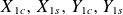 $X_{1c}, X_{1s}, Y_{1c}, Y_{1s}$
are outputs of the NAE expansion at first order.Footnote
8
The Frenet–Serret basis vectors are also known, as well as their cylindrical projections, which we denote
$X_{1c}, X_{1s}, Y_{1c}, Y_{1s}$
are outputs of the NAE expansion at first order.Footnote
8
The Frenet–Serret basis vectors are also known, as well as their cylindrical projections, which we denote
 $y^j$
for
$y^j$
for
 $y \in \{\hat {\kappa }, \hat {\tau }, \hat {b_0}\}$
and
$y \in \{\hat {\kappa }, \hat {\tau }, \hat {b_0}\}$
and
 $j \in \{R, \phi , Z\}$
denoting the cylindrical basis vector along which that Frenet–Serret basis vector is projected. With these defined, all that remains is to write the explicit forms of the projections of
$j \in \{R, \phi , Z\}$
denoting the cylindrical basis vector along which that Frenet–Serret basis vector is projected. With these defined, all that remains is to write the explicit forms of the projections of
 $\boldsymbol{x}_1$
and collect the terms attached to the
$\boldsymbol{x}_1$
and collect the terms attached to the
 $\cos \theta$
and
$\cos \theta$
and
 $\sin \theta$
terms. Writing the projections of
$\sin \theta$
terms. Writing the projections of
 $\boldsymbol{x}_1$
explicitly
$\boldsymbol{x}_1$
explicitly
 \begin{align} x_1^R &= \boldsymbol{x}_1 \boldsymbol{\cdot }\hat {R} = \cos \theta \left ( X_1^c \kappa ^R + Y_1^c \tau ^R \right ) + \sin \theta \left ( Y_1^s \tau ^R + X_1^s \kappa ^R \right )\! ,\\[-10pt]\nonumber\end{align}
 \begin{align} x_1^\phi &= \boldsymbol{x}_1 \boldsymbol{\cdot }\hat {\phi } = \cos \theta \left ( X_1^c \kappa ^{\phi } + Y_1^c \tau ^{\phi } \right ) + \sin \theta \left ( Y_1^s \tau ^{\phi } + X_1^s \kappa ^{\phi } \right )\! ,\\[-10pt]\nonumber\end{align}
 \begin{align} x_1^z &= \boldsymbol{x}_1 \boldsymbol{\cdot }\hat {Z} = \cos \theta \left ( X_1^c \kappa ^{Z} + Y_1^c \tau ^{Z} \right ) + \sin \theta \left ( Y_1^s \tau ^{Z} + X_1^s \kappa ^{Z} \right )\! .\end{align}
Plugging the above into the expressions for
 $R_1$
yields
$R_1$
yields
 \begin{align} R_1&=\mathcal{R}_{1,1}(\phi )\cos \theta +\mathcal{R}_{1,-1}(\phi )\sin \theta ,\\[-10pt]\nonumber\end{align}
 \begin{align} &=\left [X_1^c \left (\kappa ^R - \kappa ^{\phi } \frac {\partial _{\phi }R_0}{R_0}\right ) + Y_1^c \left ( \tau ^R - \tau ^{\phi }\frac {\partial _{\phi }R_0}{R_0}\right ) \right ]\cos \theta ,\\[-10pt]\nonumber\end{align}
 \begin{align} &+ \left [Y_1^s \left (\tau ^R - \tau ^\phi \frac {\partial _{\phi }R_0}{R_0}\right ) + X_1^s \left (\kappa ^R - \kappa ^\phi \frac {\partial _{\phi }R_0}{R_0}\right ) \right ] \sin \theta .\end{align}
Where we identify the terms multiplying
 $\cos \theta$
as
$\cos \theta$
as
 $\mathcal{R}_{1,1}(\phi )$
and those multiplying
$\mathcal{R}_{1,1}(\phi )$
and those multiplying
 $\sin \theta$
as
$\sin \theta$
as
 $\mathcal{R}_{1,-1}(\phi )$
. The same may be carried out for
$\mathcal{R}_{1,-1}(\phi )$
. The same may be carried out for
 $Z_1$
, yielding
$Z_1$
, yielding
 \begin{align} Z_1&=\mathcal{Z}_{1,1}(\phi )\cos \theta +\mathcal{Z}_{1,-1}(\phi )\sin \theta ,\\[-10pt]\nonumber\end{align}
 \begin{align} &=\left [X_1^c \left (\kappa ^Z - \kappa ^{\phi } \frac {\partial _{\phi }Z_0}{R_0}\right ) + Y_1^c \left ( \tau ^Z - \tau ^{\phi }\frac {\partial _{\phi }Z_0}{R_0}\right ) \right ]\cos \theta ,\\[-10pt]\nonumber\end{align}
 \begin{align} &+ \left [Y_1^s \left (\tau ^Z - \tau ^\phi \frac {\partial _{\phi }Z_0}{R_0}\right ) + X_1^s \left (\kappa ^Z - \kappa ^\phi \frac {\partial _{\phi }Z_0}{R_0}\right ) \right ] \sin \theta ,\end{align}
where again one may identify
 $\mathcal{Z}_{1,1}(\phi )$
and
$\mathcal{Z}_{1,1}(\phi )$
and
 $\mathcal{Z}_{1,-1}(\phi )$
by matching coefficients. With these quantities known as a function of the cylindrical toroidal angle
$\mathcal{Z}_{1,-1}(\phi )$
by matching coefficients. With these quantities known as a function of the cylindrical toroidal angle
 $\phi$
, the final step to arrive at the coefficients we may use to constrain the DESC Fourier–Zernike coefficients to enforce the first-order behaviour to match the NAE is to Fourier transform these quantities in
$\phi$
, the final step to arrive at the coefficients we may use to constrain the DESC Fourier–Zernike coefficients to enforce the first-order behaviour to match the NAE is to Fourier transform these quantities in
 $\phi$
to finally yield
$\phi$
to finally yield
 $\mathcal{R}_{1,1,n}, \mathcal{R}_{1,-1,n}, \mathcal{Z}_{1,1,n}, \mathcal{Z}_{1,-1,n}$
, which are then used in (3.8).
$\mathcal{R}_{1,1,n}, \mathcal{R}_{1,-1,n}, \mathcal{Z}_{1,1,n}, \mathcal{Z}_{1,-1,n}$
, which are then used in (3.8).
Appendix E. Second-order flux surface description
In this appendix we detail the derivation of the constraints related to the second-order near-axis behaviour. Let in that case
 $\boldsymbol{x}=\boldsymbol{r}_0+\rho \boldsymbol{x}_1+\rho ^2\boldsymbol{x}_2$
, where
$\boldsymbol{x}=\boldsymbol{r}_0+\rho \boldsymbol{x}_1+\rho ^2\boldsymbol{x}_2$
, where
 $\boldsymbol{x}_2=X_2\hat {\boldsymbol \kappa }+Y_2\hat {\boldsymbol \tau }+Z_2\hat {\boldsymbol{t}}$
, and consider an additional triangle defined by
$\boldsymbol{x}_2=X_2\hat {\boldsymbol \kappa }+Y_2\hat {\boldsymbol \tau }+Z_2\hat {\boldsymbol{t}}$
, and consider an additional triangle defined by
 $\boldsymbol{x}_1$
and
$\boldsymbol{x}_1$
and
 $\boldsymbol{x}_2$
. We summarise the relevant geometry in the diagram in figure 6, an extension of figure 1.
$\boldsymbol{x}_2$
. We summarise the relevant geometry in the diagram in figure 6, an extension of figure 1.
Diagram illustrating the key element for the geometric transformation at second order. Schematic diagram showing the position of a point on the surface (at radial distance
 $R$
and angle
$R$
and angle
 $\phi _0+\delta \phi$
), in reference to other quantities. These include the position along the magnetic axis (radial position
$\phi _0+\delta \phi$
), in reference to other quantities. These include the position along the magnetic axis (radial position
 $R_0$
and angle
$R_0$
and angle
 $\phi _0$
), and
$\phi _0$
), and
 $\rho \boldsymbol{x}_1$
and
$\rho \boldsymbol{x}_1$
and
 $\rho \boldsymbol{x}_2$
from the axis to the point, projected onto the
$\rho \boldsymbol{x}_2$
from the axis to the point, projected onto the
 $R,\,\phi _c$
plane (superindex
$R,\,\phi _c$
plane (superindex
 $\pi$
). The diagram to the right is a zoom-in of the triangle formed by
$\pi$
). The diagram to the right is a zoom-in of the triangle formed by
 $\{\boldsymbol{x}_1^\pi ,\boldsymbol{x}_2^\pi ,\bar {\boldsymbol{x}}\}$
.
$\{\boldsymbol{x}_1^\pi ,\boldsymbol{x}_2^\pi ,\bar {\boldsymbol{x}}\}$
.

The construction then follows identical geometric arguments to those used in the main text for the first-order construction. Define an angle
 $\phi _2$
as the angle between
$\phi _2$
as the angle between
 $\boldsymbol{x}_2^\pi$
and
$\boldsymbol{x}_2^\pi$
and
 $\boldsymbol{x}_1^\pi$
(the projection of the respective vectors onto the
$\boldsymbol{x}_1^\pi$
(the projection of the respective vectors onto the
 $Z=0$
plane), the angle
$Z=0$
plane), the angle
 $\delta \phi _2$
as the small angle of the triangle they form, with
$\delta \phi _2$
as the small angle of the triangle they form, with
 $\overline {x}$
the total length of the sum of
$\overline {x}$
the total length of the sum of
 $\boldsymbol{x}_2^\pi$
and
$\boldsymbol{x}_2^\pi$
and
 $\boldsymbol{x}_1^\pi$
. Using the sine and cosine rules
$\boldsymbol{x}_1^\pi$
. Using the sine and cosine rules
 \begin{align} \delta \phi _2\approx \frac {x_2^\pi }{x_1^\pi }\sin \phi _2, \end{align}
 \begin{align} \overline {x}-x_1^\pi \approx x_2^\pi \cos \phi _2, \end{align}
which are completely analogous to the expressions in § 3.2. Now we must consider this
 $\overline {\boldsymbol{x}}$
piece together with
$\overline {\boldsymbol{x}}$
piece together with
 $R_0$
. Define
$R_0$
. Define
 $\delta \phi$
to be the angle subtended by
$\delta \phi$
to be the angle subtended by
 $\overline {x}$
(see figure 6), and define an auxiliary angle
$\overline {x}$
(see figure 6), and define an auxiliary angle
 $\overline {\delta \phi }$
so that
$\overline {\delta \phi }$
so that
 $\overline {\delta \phi }=\delta \phi -\delta \phi _0$
, where
$\overline {\delta \phi }=\delta \phi -\delta \phi _0$
, where
 $\delta \phi _0=x_1^\phi /R_0$
is the angle correction derived at first order; that is, this barred
$\delta \phi _0=x_1^\phi /R_0$
is the angle correction derived at first order; that is, this barred
 $\delta \phi$
is the change in the angle die to the change in the angle die to the second order. From the sine rule, it follows that
$\delta \phi$
is the change in the angle die to the change in the angle die to the second order. From the sine rule, it follows that
 \begin{equation} \overline {\delta \phi } \approx \frac {x_2^\phi }{R_0}-\frac {x_1^Rx_1^\phi }{R_0^2}. \end{equation}
For the position
 $R$
, we also define a second-order correction
$R$
, we also define a second-order correction
 $\overline {\delta R}=R-R_0=\delta R_0$
, where
$\overline {\delta R}=R-R_0=\delta R_0$
, where
 $\delta R_0=x_1^R$
is the first-order form. Using
$\delta R_0=x_1^R$
is the first-order form. Using
 $\bar {x}$
in (E2), as well as
$\bar {x}$
in (E2), as well as
 $\overline {\delta \phi }$
in (E3), and applying the cosine rule
$\overline {\delta \phi }$
in (E3), and applying the cosine rule
 \begin{equation} \overline {\delta R}\approx x_2^R+\frac {(x_1^\phi )^2}{2R_0}. \end{equation}
Recall that this is not the end of the story, as we must express everything as a function of the cylindrical angle
 $\phi _c$
evaluated at the flux surface point. However, all quantities we know are functions of the position along the magnetic axis. Keeping the next-order correctionFootnote
9
$\phi _c$
evaluated at the flux surface point. However, all quantities we know are functions of the position along the magnetic axis. Keeping the next-order correctionFootnote
9
 \begin{align} R(\phi _c)&\approx R_0(\phi _c-\delta \phi _0+\delta \phi _0\partial _\phi \delta \phi _0-\overline {\delta \phi })+\delta R_0(\phi _c-\delta \phi _0) +\overline {\delta R}(\phi _c)\nonumber \\ &\approx \dots +\rho ^2\left [\frac {(\delta \phi _0)^2}{2}\partial _\phi ^2 R_0-\overline {\delta \phi }\partial _\phi R_0-\delta \phi _0\partial _\phi \delta R_0+\delta \phi _0\partial _\phi R_0\partial _\phi \delta \phi _0+\overline {\delta R}\right ]\!. \end{align}
Thus
 \begin{align} R_2 & =-\frac {1}{2}\partial _\phi ^2R_0\left (\frac {x_1^\phi }{R_0}\right )^2-\left (\frac {x_2^\phi }{R_0}-\frac {x_1^Rx_1^\phi }{R_0^2}\right )\partial _\phi R_0\nonumber \\[5pt]& \quad -\frac {x_1^\phi }{R_0}\partial _\phi \left (x_1^R-\frac {x_1^\phi }{R_0}\partial _\phi R_0\right ) +\left (x_2^R+\frac {(x_1^\phi )^2}{2R_0}\right )\!, \end{align}
which has a simple
 $\theta$
-harmonic form
$\theta$
-harmonic form
 $R_2=R_{2,0}+R_2^c\cos 2\theta +R_2^s\sin 2\theta$
.
$R_2=R_{2,0}+R_2^c\cos 2\theta +R_2^s\sin 2\theta$
.
In the case of
 $Z$
$Z$
 \begin{equation} Z_2=-\frac {1}{2}\partial _\phi ^2 Z_0\left (\frac {x_1^\phi }{R_0}\right )^2-\left (\frac {x_2^\phi }{R_0}-\frac {x_1^Rx_1^\phi }{R_0^2}\right )\partial _\phi Z_0-\frac {x_1^\phi }{R_0}\partial _\phi \left ( x_1^z-\frac {x_1^{\phi }}{R_0}\partial _\phi Z_0\right )+x_2^z. \end{equation}
Once again, we may write the
 $Z$
content as
$Z$
content as
 $Z_2=Z_{2,0}+Z_2^c\cos 2\theta +Z_2^s\sin 2\theta$
, and find the coefficients using some algebraic manipulator.
$Z_2=Z_{2,0}+Z_2^c\cos 2\theta +Z_2^s\sin 2\theta$
, and find the coefficients using some algebraic manipulator.
(Left) Fourier coefficients as a function of toroidal mode number of the
 $O(\rho )$
NAE coefficient
$O(\rho )$
NAE coefficient
 $R_{1,1}$
(top) and order-
$R_{1,1}$
(top) and order-
 $O(\rho )$
coefficient
$O(\rho )$
coefficient
 $R_{2,0}$
(bottom) from (3.8) and (3.13a
) respectively. (Right) Error in the NAE-constrained DESC solution’s rotational transform on axis as a function of the toroidal resolution of the constraint used.
$R_{2,0}$
(bottom) from (3.8) and (3.13a
) respectively. (Right) Error in the NAE-constrained DESC solution’s rotational transform on axis as a function of the toroidal resolution of the constraint used.

Appendix F. Finite-n truncation of NAE constraint
In this appendix we present some details regarding the role of the finite toroidal resolution used to represent the equilibrium in DESC. Given the finite resolution of the DESC solver, the solution is only represented by a finite number of toroidal and poloidal modes,
 $N$
and
$N$
and
 $M$
respectively. When it comes to imposing the near-axis constraints as discussed in this paper, the finite resolution in the toroidal angle is particularly intrusive, as it leads to having to discard part of the Fourier content of the near-axis field. If the high-
$M$
respectively. When it comes to imposing the near-axis constraints as discussed in this paper, the finite resolution in the toroidal angle is particularly intrusive, as it leads to having to discard part of the Fourier content of the near-axis field. If the high-
 $n$
content in the shaping of the near-axis solution is significant, one then expects the constraint to deviate from the full near-axis behaviour. Such high-
$n$
content in the shaping of the near-axis solution is significant, one then expects the constraint to deviate from the full near-axis behaviour. Such high-
 $n$
behaviour could be driven by a significantly shaped axis geometry, but also by the nonlinear nature of the near-axis system of equations. We present an example of the magnitude of the toroidal content of some near-axis shaping coefficients on the left of figure 7.
$n$
behaviour could be driven by a significantly shaped axis geometry, but also by the nonlinear nature of the near-axis system of equations. We present an example of the magnitude of the toroidal content of some near-axis shaping coefficients on the left of figure 7.
Even though any smooth periodic function must have a decaying toroidal spectrum that decays exponentially for sufficiently large
 $n$
(Stein & Shakarchi Reference Stein and Shakarchi2011, Corollary 2.4), they do so at markedly different rates at finite mode number. The slower the decay in
$n$
(Stein & Shakarchi Reference Stein and Shakarchi2011, Corollary 2.4), they do so at markedly different rates at finite mode number. The slower the decay in
 $n$
, the harder it is to represent the near-axis solution in the pseudo-spectral choice of DESC. From the figure it can be appreciated that the decay is particularly slow for the QI field. The hardship in representing QI solutions in cylindrical coordinates is well recognised in the literature, as these configurations feature axes with straight sections that are difficult to represent with
$n$
, the harder it is to represent the near-axis solution in the pseudo-spectral choice of DESC. From the figure it can be appreciated that the decay is particularly slow for the QI field. The hardship in representing QI solutions in cylindrical coordinates is well recognised in the literature, as these configurations feature axes with straight sections that are difficult to represent with
 $\phi$
(Plunk et al. Reference Plunk, Landreman and Helander2019; Rodríguez et al. Reference Rodríguez, Plunk and Jorge2025). In addition, it is also clear that convergence of second-order behaviour is markedly slower. This is to be expected, as additional
$\phi$
(Plunk et al. Reference Plunk, Landreman and Helander2019; Rodríguez et al. Reference Rodríguez, Plunk and Jorge2025). In addition, it is also clear that convergence of second-order behaviour is markedly slower. This is to be expected, as additional
 $\phi$
-derivatives occur every time one moves an order up in the near-axis construction. Allowing an arbitrary computational toroidal angle
$\phi$
-derivatives occur every time one moves an order up in the near-axis construction. Allowing an arbitrary computational toroidal angle
 $\zeta$
could help in condensing the Fourier spectra of these behaviours, as well as adopting alternative representations (Hindenlang et al. Reference Hindenlang, Plunk and Maj2024, Reference Hindenlang, Plunk and Maj2025), however, this solution will not be pursued in this work.
$\zeta$
could help in condensing the Fourier spectra of these behaviours, as well as adopting alternative representations (Hindenlang et al. Reference Hindenlang, Plunk and Maj2024, Reference Hindenlang, Plunk and Maj2025), however, this solution will not be pursued in this work.
To assess the importance of this truncation we perform the following numerical experiment: for a toroidal resolution of
 $N$
, take the lower
$N$
, take the lower
 $n\leqslant N$
 $\mathcal{O}(\rho )$
constraints and perform an equilibrium solve.Footnote
10
The resulting
$\mathcal{O}(\rho )$
constraints and perform an equilibrium solve.Footnote
10
The resulting
 $\unicode{x0394} \iota _0(n)$
is shown on the right of figure 7. The quasisymmetric cases converge quite rapidly (
$\unicode{x0394} \iota _0(n)$
is shown on the right of figure 7. The quasisymmetric cases converge quite rapidly (
 $n\sim 5$
), suggesting in these scenarios this to be a relatively minor problem (at least at first order). In the QI case, the requirement is clearly stronger, exemplifying the complications arising from the poor representation of the field. Note, however, that the saturation of the solution must then come from the approximate form of force balance. In fact, the error does not even behave in a monotonic fashion, although it remains below a more than satisfactory level.
$n\sim 5$
), suggesting in these scenarios this to be a relatively minor problem (at least at first order). In the QI case, the requirement is clearly stronger, exemplifying the complications arising from the poor representation of the field. Note, however, that the saturation of the solution must then come from the approximate form of force balance. In fact, the error does not even behave in a monotonic fashion, although it remains below a more than satisfactory level.
Quantitative measures for precise QH aspect ratio scan. Table including the verification measures introduced in § 4.1 comparing the near-axis-constrained (NAE) and the fixed-boundary (Surf) equilibria of the precise QH (Landreman & Paul Reference Landreman and Paul2022) configuration at different aspect ratios. The first column shows the aspect ratio of the equilibria considered. One can observe that the fixed-boundary error with the NAE decreases with increasing aspect ratio, but still fares worse than the NAE-constrained equilibria.

Appendix G. The NAE constraint at extreme aspect ratios
In this appendix, two cases of the NAE constraint at extreme aspect ratios are presented, showing that the constraint performs well at both very high and very low aspect ratios.
First, the precise QH
 $\mathcal{O}({\rho })$
example from § 5 is solved at two higher aspect ratios,
$\mathcal{O}({\rho })$
example from § 5 is solved at two higher aspect ratios,
 $A\sim 9$
and
$A\sim 9$
and
 $A\sim 90$
, showcasing how high an aspect ratio is required before the fixed-boundary solution agreement with the NAE approaches the level shown in the NAE-constrained equilibria. The NAE surfaces, fixed-surface and NAE-constrained solutions are plotted in figure 8, while the NAE verification quantities are shown in table 3. The fixed-boundary solution errors with respect to the near axis grow smaller as the aspect ratio increases, consistent with previous investigations (Landreman & Sengupta Reference Landreman and Sengupta2019), but still at aspect ratio
$A\sim 90$
, showcasing how high an aspect ratio is required before the fixed-boundary solution agreement with the NAE approaches the level shown in the NAE-constrained equilibria. The NAE surfaces, fixed-surface and NAE-constrained solutions are plotted in figure 8, while the NAE verification quantities are shown in table 3. The fixed-boundary solution errors with respect to the near axis grow smaller as the aspect ratio increases, consistent with previous investigations (Landreman & Sengupta Reference Landreman and Sengupta2019), but still at aspect ratio
 $\sim 90$
fail to match even the smallest aspect ratio (
$\sim 90$
fail to match even the smallest aspect ratio (
 $\sim 4$
) NAE-constrained equilibrium’s errors. The NAE-constrained equilibrium consistently outperforms the fixed-boundary equilibrium at each aspect ratio presented.
$\sim 4$
) NAE-constrained equilibrium’s errors. The NAE-constrained equilibrium consistently outperforms the fixed-boundary equilibrium at each aspect ratio presented.
First-order precise QH aspect ratio scan. The figure shows a comparison of DESC first-order NAE-constrained equilibrium solutions (in red) against DESC near-axis fixed-boundary solutions (in green) and the ideal near-axis field (broken line). From left to right the configurations correspond to precise QH at increasing aspect ratios (corresponding to evaluated boundary radii of
 $r=0.2$
,
$r=0.2$
,
 $r=0.1$
and
$r=0.1$
and
 $r=0.01$
). (Top) Cross-sections at
$r=0.01$
). (Top) Cross-sections at
 $\phi =0$
. (Middle) Rotational transform profile showing the correct matching of the NAE-constrained field. (Bottom) The left plots show the Boozer quasisymmetry metric for the QS solutions (measure of
$\phi =0$
. (Middle) Rotational transform profile showing the correct matching of the NAE-constrained field. (Bottom) The left plots show the Boozer quasisymmetry metric for the QS solutions (measure of
 $|\boldsymbol{B}|$
error). The fixed-boundary equilibria better match the NAE as the aspect ratio is increased, with the sum of QS symmetry breaking modes showing the expected
$|\boldsymbol{B}|$
error). The fixed-boundary equilibria better match the NAE as the aspect ratio is increased, with the sum of QS symmetry breaking modes showing the expected
 $\sim A^{-2}$
scaling (most evident when comparing the bottom middle and right plots), although the NAE-constrained equilibria remain a better match at each aspect ratio. The QH equilibria were solved at a resolution of
$\sim A^{-2}$
scaling (most evident when comparing the bottom middle and right plots), although the NAE-constrained equilibria remain a better match at each aspect ratio. The QH equilibria were solved at a resolution of
 $L=10,\,M=10,\,N=24$
.
$L=10,\,M=10,\,N=24$
.

Second, a finite-beta (beta being the ratio of plasma pressure to magnetic pressure), four field-period QH NAE solution (detailed in Section 5.4 of Landreman (Reference Landreman2022a ) and obtainable from pyQSC as ‘2022 QH nfp4 Mercier’) is presented as demonstration of two capabilities: the performance of the NAE constraint at aspect ratios where the NAE begins to break down, and obtaining Mercier stability (Mercier Reference Mercier1962, Reference Mercier1974; Greene & Johnson Reference Greene and Johnson1962; Bauer, Betancourt & Garabedian Reference Bauer, Betancourt and Garabedian2012; Freidberg Reference Freidberg2014) near axis without optimisation.
As detailed in the literature (Landreman Reference Landreman2021), there exist various NAE metrics used to assess the expansion’s regime of validity. One such metric is
 $r_c$
, defined as the radius at which the
$r_c$
, defined as the radius at which the
 $\mathcal{O}(\rho ^2)$
NAE surfaces begin to exhibit pathological behaviour such as self-intersection (and thus the region where the NAE second-order solution begins to break down). One expects the NAE solution to no longer accurately approximate the global equilibrium when evaluated near this radius.
$\mathcal{O}(\rho ^2)$
NAE surfaces begin to exhibit pathological behaviour such as self-intersection (and thus the region where the NAE second-order solution begins to break down). One expects the NAE solution to no longer accurately approximate the global equilibrium when evaluated near this radius.
The chosen QH configuration in this appendix has
 $r_c\sim 0.1\,\text{m}$
and we evaluate the NAE surfaces at an aspect ratio corresponding to
$r_c\sim 0.1\,\text{m}$
and we evaluate the NAE surfaces at an aspect ratio corresponding to
 $r \sim 0.1\,\text{m}$
, thus evaluating the NAE where it is clearly no longer a good approximation to the global equilibrium. We use the same second-order NAE constraints, resolutions and procedure as described in § 5.2, and show the results for the fixed-surface and fixed-NAE equilibria in figure 9. The results show that the NAE-constrained equilibrium, while closely adhering to the NAE solution near axis, allows large deviations of the flux surface geometry away from the axis in order to satisfy force balance (much larger deviations than seen in figure 5), in line with the second-order NAE surfaces not being an accurate approximation of a global equilibrium solution at this radius, as predicted by
$r \sim 0.1\,\text{m}$
, thus evaluating the NAE where it is clearly no longer a good approximation to the global equilibrium. We use the same second-order NAE constraints, resolutions and procedure as described in § 5.2, and show the results for the fixed-surface and fixed-NAE equilibria in figure 9. The results show that the NAE-constrained equilibrium, while closely adhering to the NAE solution near axis, allows large deviations of the flux surface geometry away from the axis in order to satisfy force balance (much larger deviations than seen in figure 5), in line with the second-order NAE surfaces not being an accurate approximation of a global equilibrium solution at this radius, as predicted by
 $r_c$
. The NAE-constrained solution also retains a stable magnetic well (across the entirety of the volume, and matching the NAE on axis) as well as Mercier stability near the core (adhering closely to that computed by the NAE solution (Landreman & Jorge Reference Landreman and Jorge2020) near the core). The fixed-surface solution, in contrast, has an on-axis iota that is off by almost 50 % compared with the NAE, as well as on-axis instability in both the magnetic well and Mercier metrics. This shows both an example of the NAE constraint retaining near-axis Mercier stability in a global equilibrium without optimisation, and its ability to perform well even at aspect ratios where the NAE is clearly no longer a good approximation of the global solution.
$r_c$
. The NAE-constrained solution also retains a stable magnetic well (across the entirety of the volume, and matching the NAE on axis) as well as Mercier stability near the core (adhering closely to that computed by the NAE solution (Landreman & Jorge Reference Landreman and Jorge2020) near the core). The fixed-surface solution, in contrast, has an on-axis iota that is off by almost 50 % compared with the NAE, as well as on-axis instability in both the magnetic well and Mercier metrics. This shows both an example of the NAE constraint retaining near-axis Mercier stability in a global equilibrium without optimisation, and its ability to perform well even at aspect ratios where the NAE is clearly no longer a good approximation of the global solution.
Verification of Mercier stability in second-order NAE-constrained equilibrium with pressure. The figure shows a comparison of DESC second-order NAE-constrained equilibrium solution (in red) against DESC fixed-boundary solutions (in green) and the ideal near-axis field (broken line) for a QH finite-beta NAE solution which exhibits on-axis Mercier stability. (Left) Cross-sections at
 $\phi =0$
. (Middle upper) Rotational transform profile showing the correct matching of the NAE-constrained field. (Middle lower) Boozer quasisymmetry metric for the QS solutions (measure of
$\phi =0$
. (Middle upper) Rotational transform profile showing the correct matching of the NAE-constrained field. (Middle lower) Boozer quasisymmetry metric for the QS solutions (measure of
 $|\boldsymbol{B}|$
error). The NAE-constrained equilibrium adheres closely to the expected cubic scaling. (Right upper) Magnetic well parameter, where the NAE-constrained solution matches the (stable) NAE value on-axis. (Right lower) The Mercier stability parameter, where the DESC NAE-constrained equilibrium follows the expected (stable) value as computed from the NAE solution near axis. The equilibrium was solved in DESC at radial (
$|\boldsymbol{B}|$
error). The NAE-constrained equilibrium adheres closely to the expected cubic scaling. (Right upper) Magnetic well parameter, where the NAE-constrained solution matches the (stable) NAE value on-axis. (Right lower) The Mercier stability parameter, where the DESC NAE-constrained equilibrium follows the expected (stable) value as computed from the NAE solution near axis. The equilibrium was solved in DESC at radial (
 $L$
), poloidal (
$L$
), poloidal (
 $M$
) and toroidal (
$M$
) and toroidal (
 $N$
) spectral resolutions of
$N$
) spectral resolutions of
 $L=15,\,M=10,\,N=25$
, and the near-axis solution using pyQSC.
$L=15,\,M=10,\,N=25$
, and the near-axis solution using pyQSC.


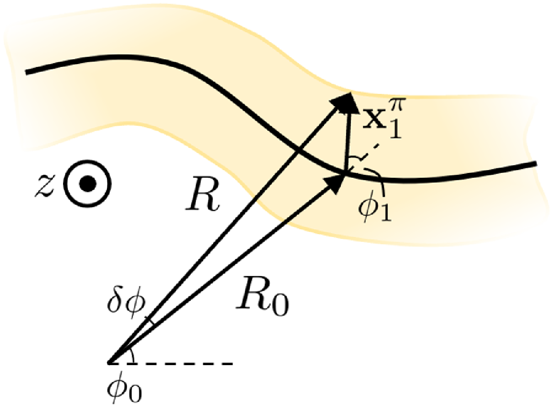


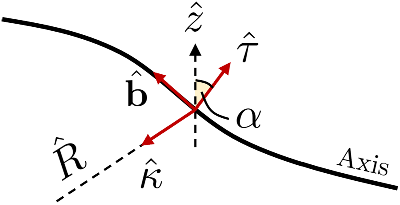


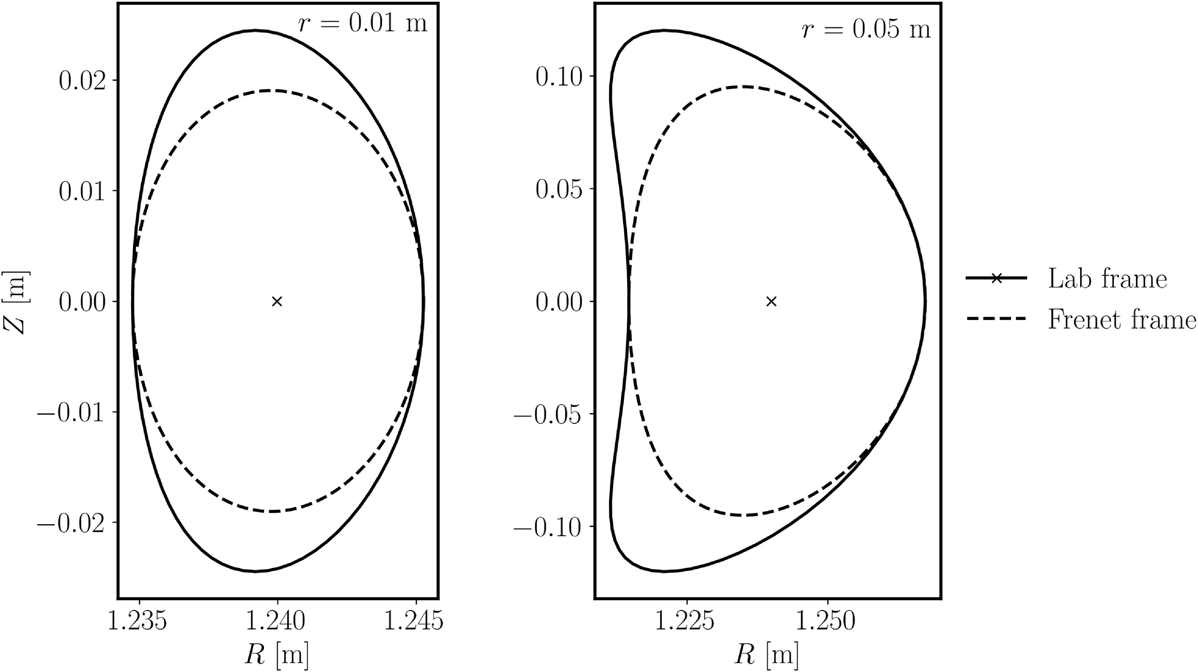


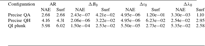
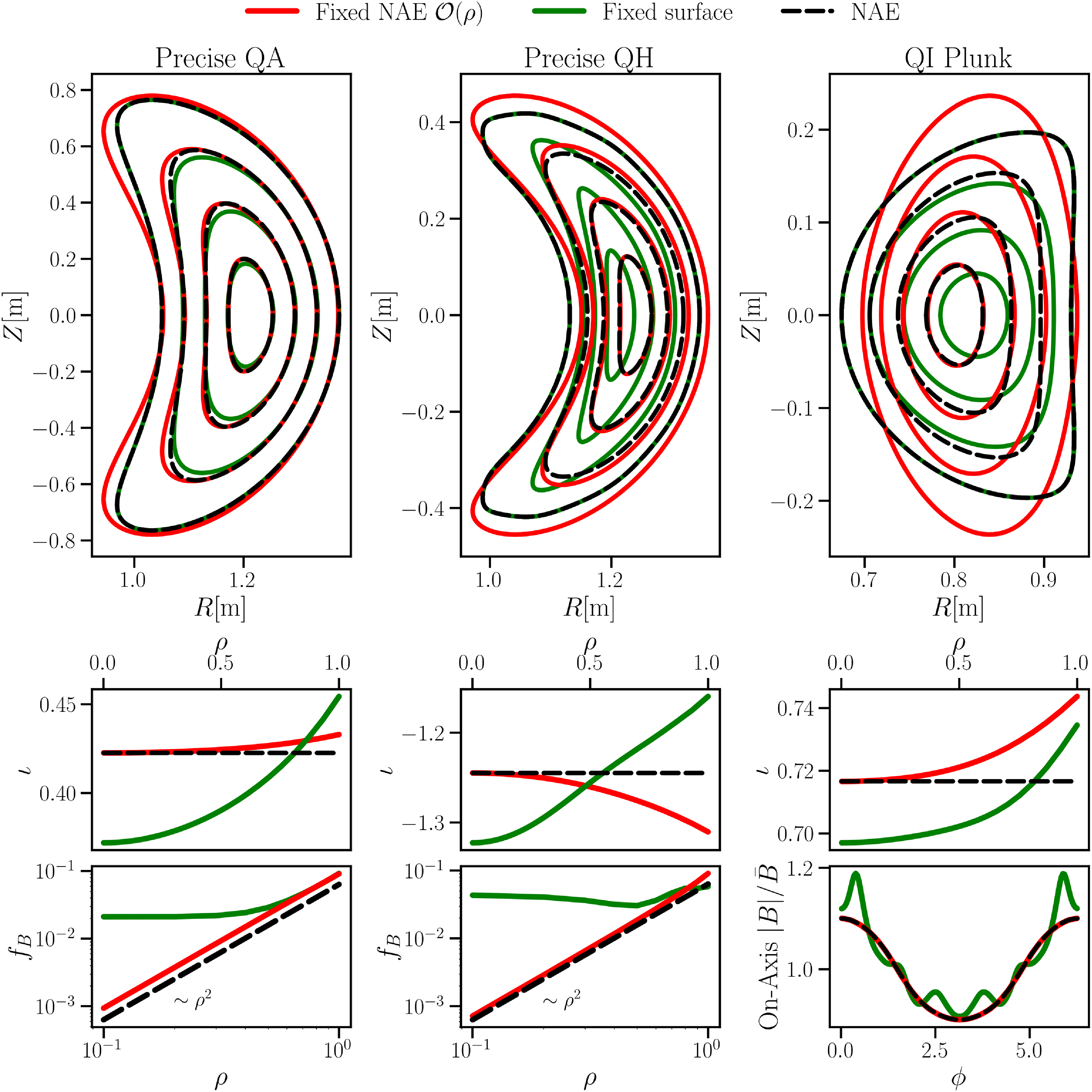


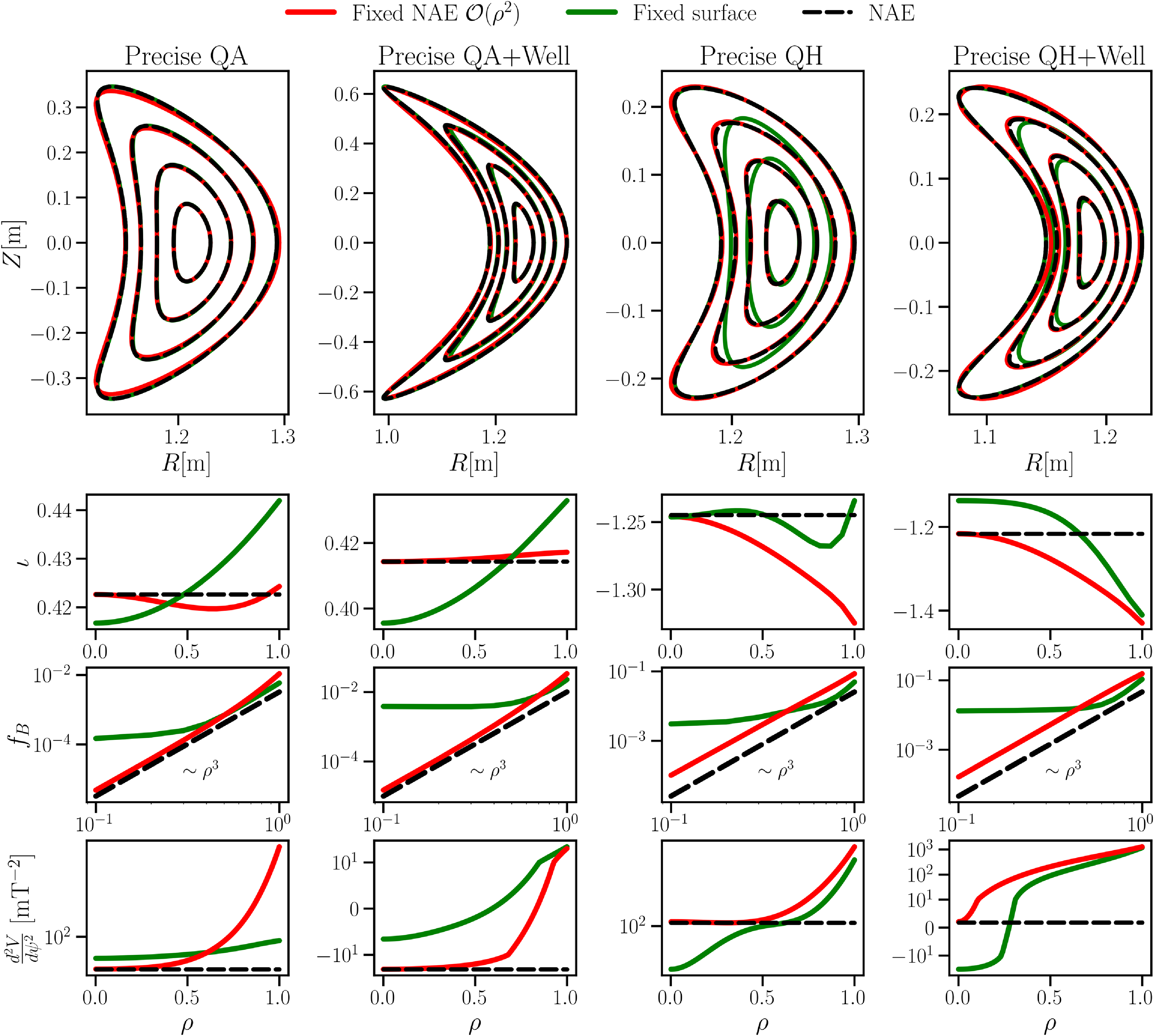


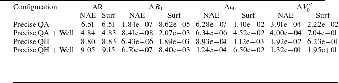
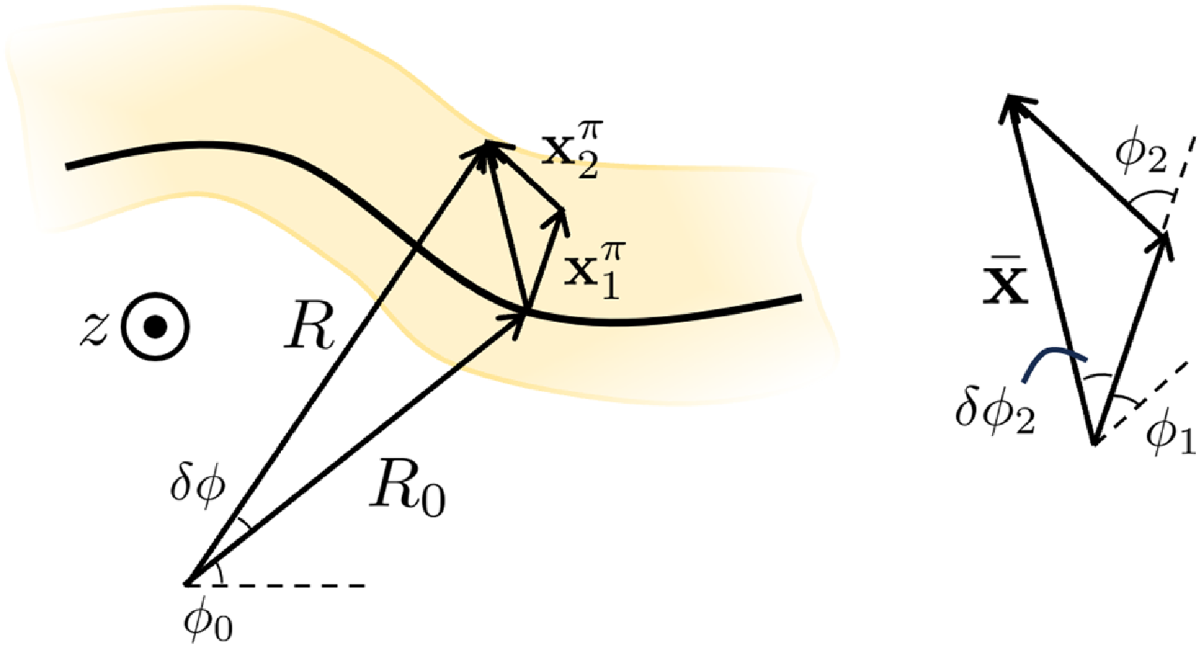


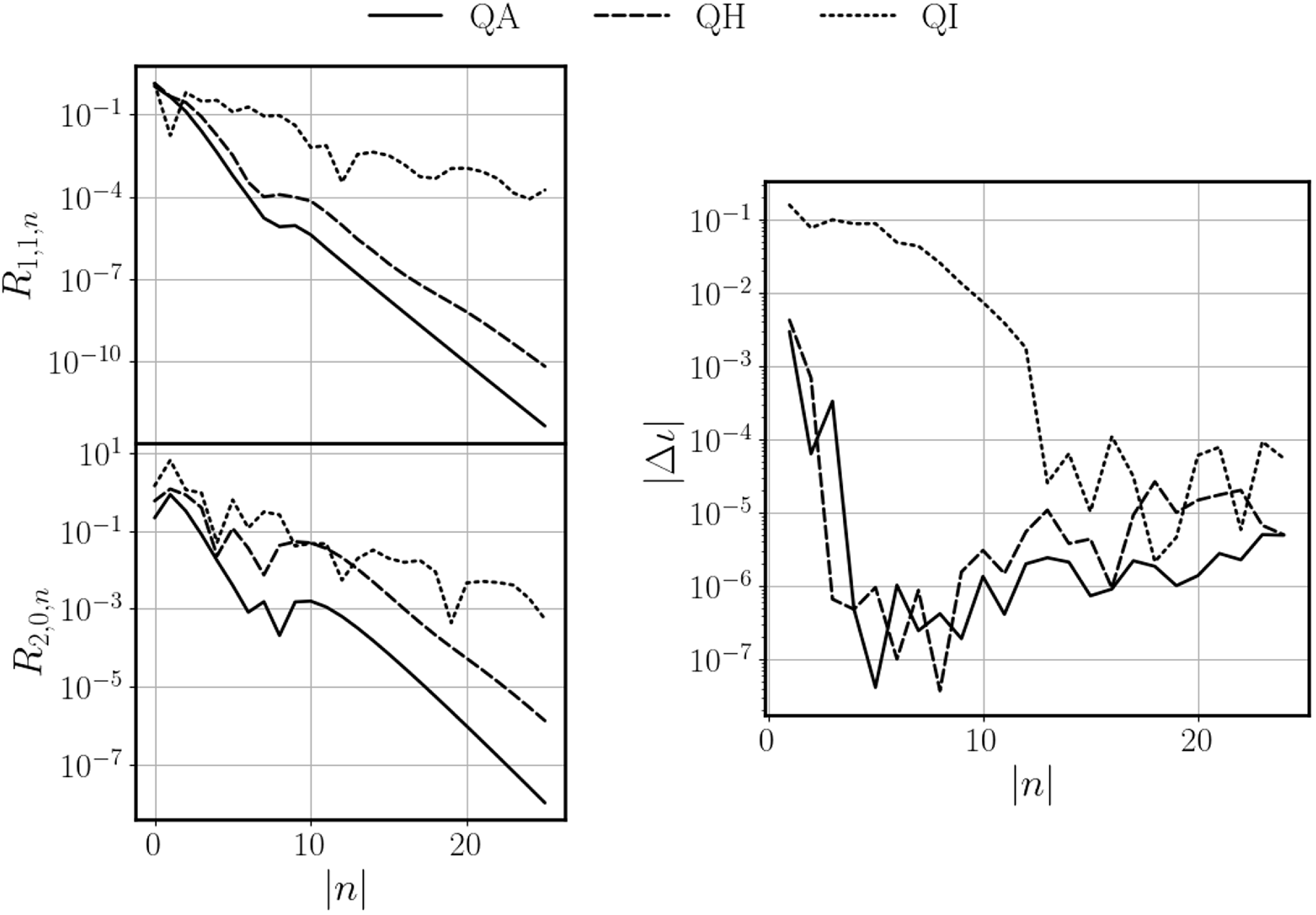


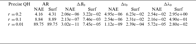
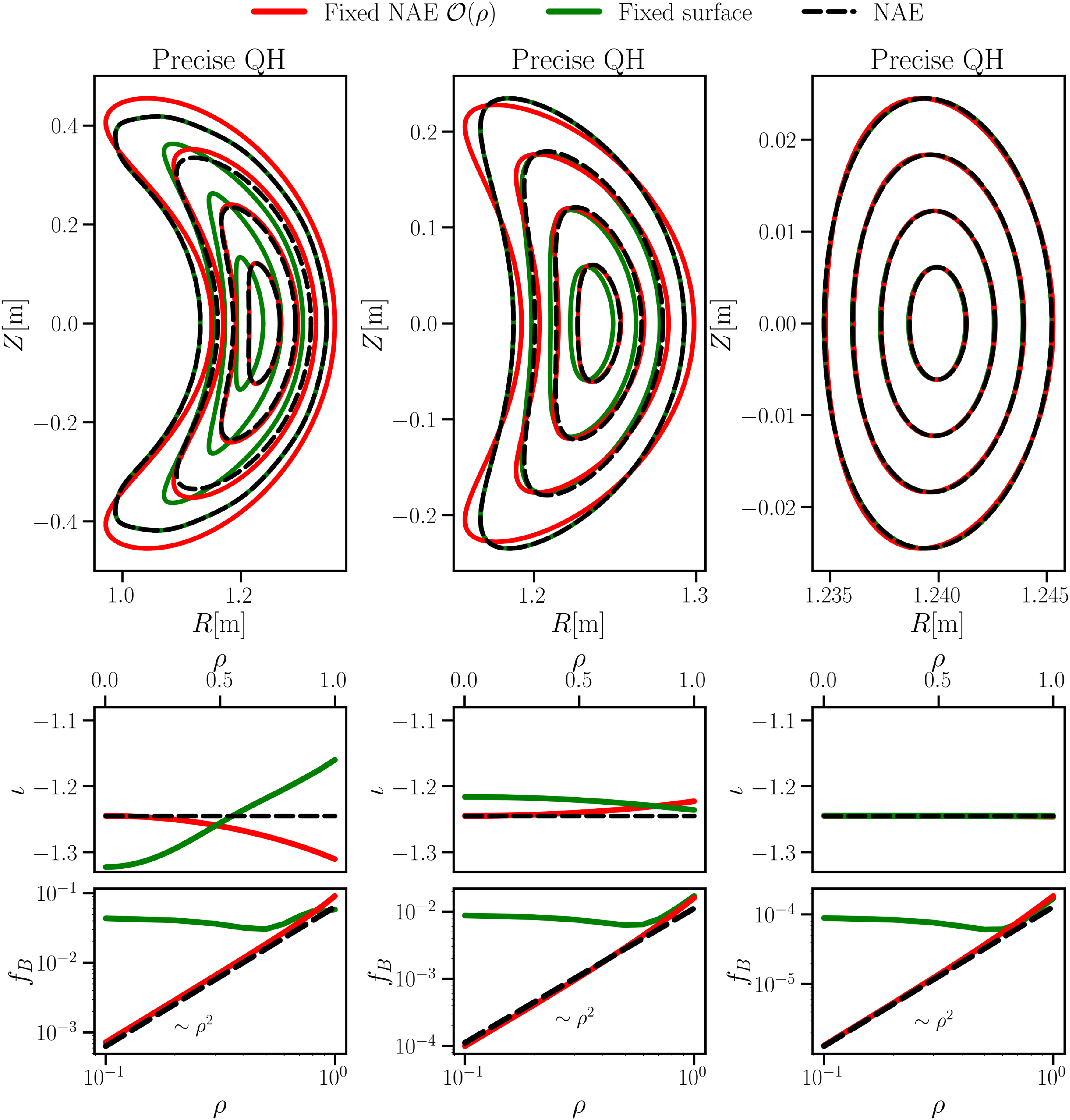


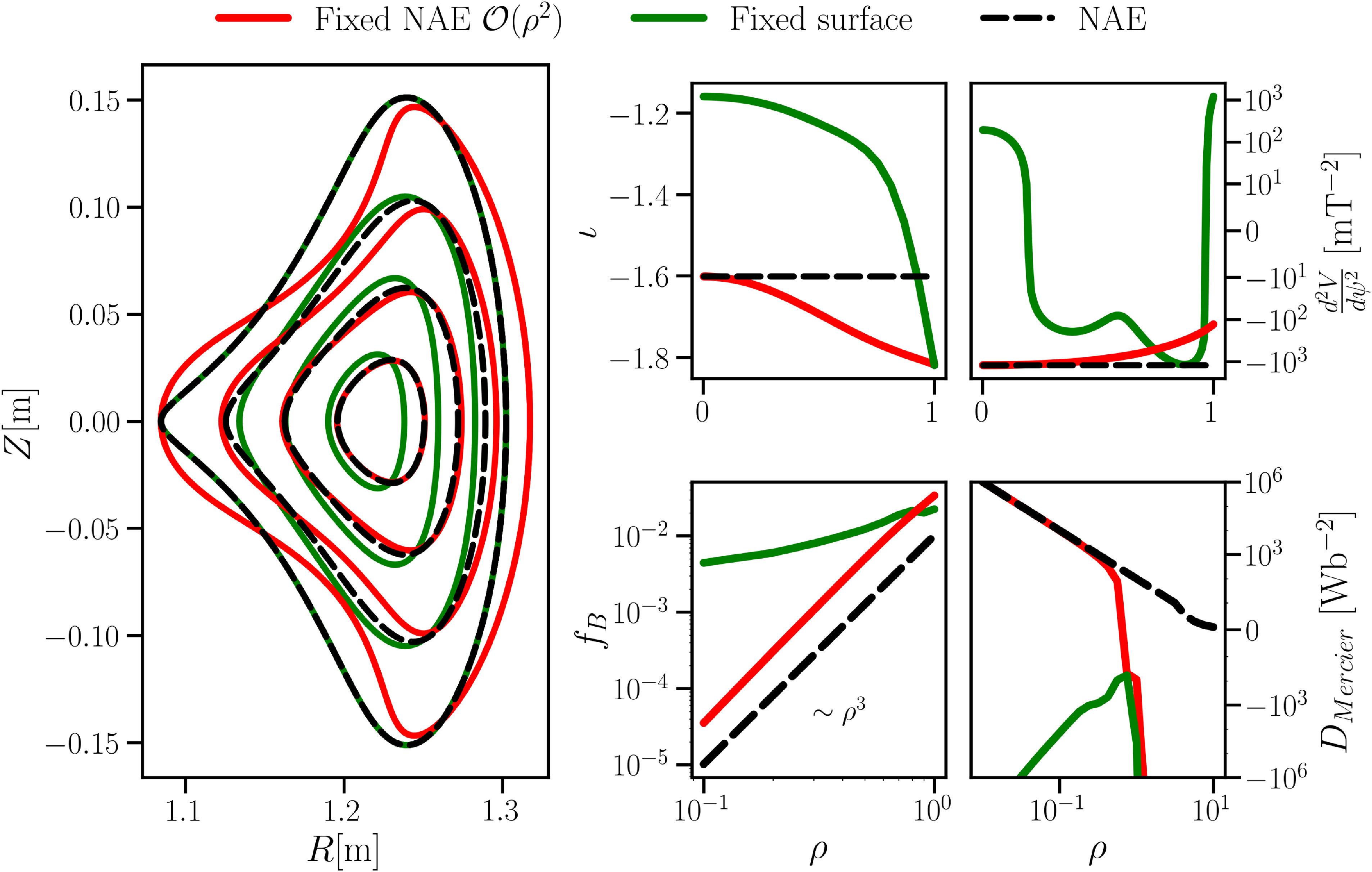


 Open access