


1. Introduction
The ubiquity of unsteady phenomena in nature is well-established, particularly in the context of the accelerating motion of organisms within fluid environments. These organisms, such as flyers and swimmers, exhibit behaviours characterized by the acceleration and morphing of wings, fins and bodies (Mountcastle & Combes Reference Mountcastle and Combes2013; Lucas et al. Reference Lucas, Johnson, Beaulieu, Cathcart, Tirrell, Colin, Gemmell, Dabiri and Costello2014; Chin & Lentink Reference Chin and Lentink2016; Triantafyllou, Weymouth & Miao Reference Triantafyllou, Weymouth and Miao2016) and, particularly, morphing provides additional benefits. For example, insects enhance their flapping efficiency through the passive deformation of their wings (Ho et al. Reference Ho, Nassef, Pornsinsirirak, Tai and Ho2003; Kang et al. Reference Kang, Aono, Cesnik and Shyy2011; Kang & Shyy Reference Kang and Shyy2013), birds coordinate flight efficiency (Johansson, Wolf & Hedenström Reference Johansson, Wolf and Hedenström2010; Taylor et al. Reference Taylor, Carruthers, Hubel and Walker2012) and disturbance resistance (Reynolds, Thomas & Taylor Reference Reynolds, Thomas and Taylor2014; Harvey et al. Reference Harvey, Baliga, Lavoie and Altshuler2019; Cheney et al. Reference Cheney, Stevenson, Durston, Song, Usherwood, Bomphrey and Windsor2020) through active wing morphing, and marine swimmers utilize fin flexibility to enhance propulsion efficiency or to gain high acceleration during manoeuvres (Triantafyllou et al. Reference Triantafyllou, Weymouth and Miao2016; Hang et al. Reference Hang, Heydari, Costello and Kanso2022; Jimenez et al. Reference Jimenez, Lucas, Long and Tytell2023). Direct simulations or experiments provide detailed insights into these phenomena; however, due to the inherent complexity of modelling, the generality of the derived fluid dynamic laws remains limited (Ho et al. Reference Ho, Nassef, Pornsinsirirak, Tai and Ho2003; Kang et al. Reference Kang, Aono, Cesnik and Shyy2011; Ramananarivo, Godoy-Diana & Thiria Reference Ramananarivo, Godoy-Diana and Thiria2011; Kang & Shyy Reference Kang and Shyy2013). Therefore, researchers tend to abstract moving appendages as plates in model problems to reveal universal fluid dynamic laws (Kim & Gharib Reference Kim and Gharib2011b ; Fernando & Rival Reference Fernando and Rival2016b ; Reijtenbagh et al. Reference Reijtenbagh, Tummers and Westerweel2023a ; Li et al. Reference Li, Chen, Xiang, Liu and Wang2024).
Considering that any unsteady motion (neglecting rotation) can be approximated by superposing small intervals of uniformly accelerated motions (Kaiser, Kriegseis & Rival Reference Kaiser, Kriegseis and Rival2020; Li et al. Reference Li, Xiang, Qin, Liu and Wang2022) and reconfigurable plates abstract the geometry of wings and fins (Kim & Gharib Reference Kim and Gharib2011a , Reference Kim and Gharibb ), accelerating reconfigurable circular plates, which incorporate both acceleration and shape deformation, are adopted as a fundamental model to investigate the unsteady fluid-dynamic forces and flow field for biological propulsion and disturbance resistance.
The influence of acceleration on the force evolution of rigid circular plates is first discussed, which has been extensively investigated (Fernando & Rival Reference Fernando and Rival2016b
; Reijtenbagh et al. Reference Reijtenbagh, Tummers and Westerweel2023a
; Li et al. Reference Li, Chen, Xiang, Liu and Wang2024). The force evolution exhibits a distinct ‘peak-and-valley’ pattern: during the acceleration process, the force increases with velocity, peaks at the end of acceleration and then gradually decreases to a valley as acceleration ceases, before slowly rising until stabilizing. The instantaneous force decreasing to a minimum before increasing again to reach a steady value is known as the ‘drag trough’ phenomenon (Fernando & Rival Reference Fernando and Rival2016a
). Two dynamic parameters govern the force scaling for such plates: the Reynolds number,
 $ Re = \rho _{\!f} U_c D/\mu$
, and the acceleration number,
$ Re = \rho _{\!f} U_c D/\mu$
, and the acceleration number,
 $ a^* = a D/U_c^2$
, where
$ a^* = a D/U_c^2$
, where
 $ D$
,
$ D$
,
 $ a$
and
$ a$
and
 $ U_c$
are the characteristic length, acceleration and velocity of the translating plate, respectively, and
$ U_c$
are the characteristic length, acceleration and velocity of the translating plate, respectively, and
 $ \rho _{\!f}$
and
$ \rho _{\!f}$
and
 $ \mu$
are the density and dynamic viscosity of the fluid. For rigid circular plates, the force evolution exhibits Reynolds number independence within the range of
$ \mu$
are the density and dynamic viscosity of the fluid. For rigid circular plates, the force evolution exhibits Reynolds number independence within the range of
 $ 50\,000 \leqslant Re \leqslant 350\,000$
when the dimensionless travel distance is less than
$ 50\,000 \leqslant Re \leqslant 350\,000$
when the dimensionless travel distance is less than
 $6$
(Fernando & Rival Reference Fernando and Rival2016b
). Additionally, an
$6$
(Fernando & Rival Reference Fernando and Rival2016b
). Additionally, an
 $ a^*$
dependence exists, indicating that for the same
$ a^*$
dependence exists, indicating that for the same
 $ a^*$
conditions, the instantaneous force evolution follows a consistent pattern regardless of variations in actual characteristic acceleration
$ a^*$
conditions, the instantaneous force evolution follows a consistent pattern regardless of variations in actual characteristic acceleration
 $ a$
and velocity
$ a$
and velocity
 $ U_c$
(Fernando & Rival Reference Fernando and Rival2016b
; Li et al. Reference Li, Xiang, Qin, Liu and Wang2022).
$ U_c$
(Fernando & Rival Reference Fernando and Rival2016b
; Li et al. Reference Li, Xiang, Qin, Liu and Wang2022).
Two perspectives are commonly used to explain the unsteady mechanisms of force generation during the acceleration of a rigid flat plate from rest: the quasisteady view (Fernando & Rival Reference Fernando and Rival2016a , Reference Fernando and Rivalb ; Reijtenbagh et al. Reference Reijtenbagh, Tummers and Westerweel2023a ; Liu & Sun Reference Liu and Sun2024; Li et al. Reference Li, Chen, Xiang, Liu and Wang2024) and the impulse-based view (Kim & Gharib Reference Kim and Gharib2011a ; Li et al. Reference Li, Xiang, Qin, Liu and Wang2022). The quasisteady view, which is primarily focused on predictive modelling, decomposes the instantaneous force into a steady-state force, added-mass force and history force (Stokes Reference Stokes1851; Basset Reference Basset1888; Oseen Reference Oseen1927; Odar & Hamilton Reference Odar and Hamilton1964). While powerful, accurately modelling these terms in viscous, separated flows is challenging, as simple potential-flow models often fail (Grift et al. Reference Grift, Vijayaragavan, Tummers and Westerweel2019; Fernando, Weymouth & Rival Reference Fernando, Weymouth and Rival2020; Li et al. Reference Li, Xiang, Qin, Liu and Wang2022). This has led to an ongoing debate about the best approach: some researchers propose a variable added-mass coefficient to account for real fluid effects (Odar & Hamilton Reference Odar and Hamilton1964; McPhaden & Rival Reference McPhaden and Rival2018; Galler, Weymouth & Rival Reference Galler, Weymouth and Rival2021), while others introduce a complex history force term to capture the history of the wake, with recent work proposing new scaling laws based on this concept (Reijtenbagh et al. Reference Reijtenbagh, Tummers and Westerweel2023a ; Li et al. Reference Li, Chen, Xiang, Liu and Wang2024). In contrast, the impulse-based perspective offers a more direct link to the physical mechanisms by focusing on the evolution of the vorticity field, particularly through the vorticity moment theorem (Wu Reference Wu1981; Graham et al. Reference Graham, Pitt Ford and Babinsky2017; Kaiser et al. Reference Kaiser, Kriegseis and Rival2020). This approach posits that the force is governed by the growth of vorticity, which can be conceptually separated into added-mass vorticity and the shed vorticity that forms the wake (Corkery Reference Corkery2019). The dynamics of this shed vorticity, typically modelled as a growing vortex ring, are considered central to explaining the force history. For instance, the phenomenon of Reynolds number independence has been linked to the timing of vortex ring pinch-off (Fernando & Rival Reference Fernando and Rival2016b ), and recent models have successfully predicted instantaneous forces by tracking the details of vortex ring growth (Li et al. Reference Li, Xiang, Qin, Liu and Wang2022; Reijtenbagh et al. Reference Reijtenbagh, Tummers and Westerweel2023a ). In essence, while the quasisteady framework provides a structure for force prediction, the impulse-based view excels at providing a mechanistic explanation rooted in the observable dynamics of the wake.
Another key characteristic of accelerating reconfigurable circular plates is reconfiguration. As a standard model for morphing problems, the study of reconfigurable flat plates has previously focused primarily on steady-state conditions, where the free stream velocity is kept constant. A well-known initial study in this area is Vogel’s work (Vogel Reference Vogel1989), in which he measured the drag of leaves in a steady wind field as a function of wind speed and found that, contrary to the commonly assumed quadratic force-speed relationship, deformable leaves exhibit a power law with an exponent of
 $4/3$
in the relationship between force and wind speed. This phenomenon inspired a series of subsequent studies, particularly scaling analyses of the exponent (De Langre Reference De Langre2008). Notable works include Alben et al. (Reference Alben, Shelley and Zhang2002, Reference Alben, Shelley and Zhang2004), who used soap film experiments in two-dimensional (2-D) flow fields to measure one-dimensional (1-D) fibres, modelled based on beam theory, and defined a dimensionless length that physically represents the ratio of fluid dynamics to elastic force. Schouveiler & Boudaoud (Reference Schouveiler and Boudaoud2006) investigated the plate reconfiguration based on cone shapes, Gosselin et al. (Reference Gosselin, De Langre and Machado-Almeida2010) analysed rectangular plates and, more recently, Baskaran, Hutin & Mulleners (Reference Baskaran, Hutin and Mulleners2023) studied bioinspired flexible disks, each discovering similar power law phenomena. However, in all these configurations, force decreases compared with rigid plates due to deformation-induced area reduction and streamlining (Gosselin et al. Reference Gosselin, De Langre and Machado-Almeida2010; Baskaran et al. Reference Baskaran, Hutin and Mulleners2023).
$4/3$
in the relationship between force and wind speed. This phenomenon inspired a series of subsequent studies, particularly scaling analyses of the exponent (De Langre Reference De Langre2008). Notable works include Alben et al. (Reference Alben, Shelley and Zhang2002, Reference Alben, Shelley and Zhang2004), who used soap film experiments in two-dimensional (2-D) flow fields to measure one-dimensional (1-D) fibres, modelled based on beam theory, and defined a dimensionless length that physically represents the ratio of fluid dynamics to elastic force. Schouveiler & Boudaoud (Reference Schouveiler and Boudaoud2006) investigated the plate reconfiguration based on cone shapes, Gosselin et al. (Reference Gosselin, De Langre and Machado-Almeida2010) analysed rectangular plates and, more recently, Baskaran, Hutin & Mulleners (Reference Baskaran, Hutin and Mulleners2023) studied bioinspired flexible disks, each discovering similar power law phenomena. However, in all these configurations, force decreases compared with rigid plates due to deformation-induced area reduction and streamlining (Gosselin et al. Reference Gosselin, De Langre and Machado-Almeida2010; Baskaran et al. Reference Baskaran, Hutin and Mulleners2023).
Thus, an important question arises: Is the force exerted by an accelerating reconfigurable circular plate smaller than that of a rigid plate? If so, how can previous studies justify the benefits of flexibility in enhancing propulsion and manoeuvrability? If not, what is the underlying flow mechanism responsible for the force enhancement? Limited studies in this area include Kim & Gharib (Reference Kim and Gharib2011b ), who observed that a flexible plate generates lower forces after acceleration compared with a rigid plate but larger forces after the initial peak, attributing this behaviour to the slow development of the vortex structure. And, Joshi & Bhattacharya (Reference Joshi and Bhattacharya2022) investigated the unsteady force response of an accelerating flat plate with controlled spanwise bending and found that unsteady drag increased when the plate bent towards the incoming flow, as the growth of circulation was faster and the tip vortices remained closer to the plate during the bend-down motion. Nevertheless, while the hydrodynamics of rigid accelerating bodies (Lorite-Díez et al. Reference Lorite-Díez, Jiménez-González, Gutiérrez-Montes and Martínez-Bazán2018; Reijtenbagh et al. Reference Reijtenbagh, Tummers and Westerweel2023a ; Liu & Sun Reference Liu and Sun2024) and flexible bodies in steady flow (Vogel Reference Vogel1989; Alben, Shelley & Zhang Reference Alben, Shelley and Zhang2002; Schouveiler & Eloy Reference Schouveiler and Eloy2013; Baskaran et al. Reference Baskaran, Hutin and Mulleners2023) are increasingly understood, a systematic understanding of the governing dimensionless parameters and the key flow mechanisms for passive reconfiguration, accelerating bodies remains elusive. This motivates a deeper investigation, particularly one that leverages an impulse-based view to connect the force evolution directly to the underlying vortex dynamics.
The purpose of this study is thus to investigate the temporal evolution of force to analyse dimensionless number dependence and explore the underlying mechanism using a vortex-based low-order force model within the Reynolds number range
 $ 3.12\times 10^4 \leqslant Re \leqslant 10.8\times 10^4$
and bending stiffness range
$ 3.12\times 10^4 \leqslant Re \leqslant 10.8\times 10^4$
and bending stiffness range
 $ 4.19\times 10^{-4} \leqslant EI \leqslant 26.8$
N m (defined in § 2.2). A high-resolution force transducer and time-resolved particle image velocimetry (PIV) are the primary research methods. The article is organized as follows: § 2 introduces the experimental methods; § 3 presents the force evolution laws; § 4 discusses the flow patterns; § 5 examines the mechanisms behind the force evolution. Concluding remarks are provided in § 6.
$ 4.19\times 10^{-4} \leqslant EI \leqslant 26.8$
N m (defined in § 2.2). A high-resolution force transducer and time-resolved particle image velocimetry (PIV) are the primary research methods. The article is organized as follows: § 2 introduces the experimental methods; § 3 presents the force evolution laws; § 4 discusses the flow patterns; § 5 examines the mechanisms behind the force evolution. Concluding remarks are provided in § 6.
2. Methods
2.1. Experimental set-up
The experiments were conducted in a towing tank with a cross-sectional area of 1 m
 $\times$
1.3 m and a towing length of 2.8 m at Shanghai Jiao Tong University, as shown in figure 1 and also referenced in Li et al. (Reference Li, Xiang, Qin, Liu and Wang2022, Reference Li, Chen, Xiang, Liu and Wang2024). The tank was filled with water (
$\times$
1.3 m and a towing length of 2.8 m at Shanghai Jiao Tong University, as shown in figure 1 and also referenced in Li et al. (Reference Li, Xiang, Qin, Liu and Wang2022, Reference Li, Chen, Xiang, Liu and Wang2024). The tank was filled with water (
 $\rho _{\!f} = 1.0 \times 10^3$
kg m−
$\rho _{\!f} = 1.0 \times 10^3$
kg m−
 $^3$
) to a depth of 1.2 m. The plate with
$^3$
) to a depth of 1.2 m. The plate with
 $D = 0.10$
m was towed along the
$D = 0.10$
m was towed along the
 $x$
-axis by mounting it perpendicular to a horizontal cylindrical rod of the L-shaped sting, positioned
$x$
-axis by mounting it perpendicular to a horizontal cylindrical rod of the L-shaped sting, positioned
 $5D$
away from the free surface to minimize its influence (Grift et al. Reference Grift, Vijayaragavan, Tummers and Westerweel2019; Joshi & Bhattacharya Reference Joshi and Bhattacharya2022). An aluminium bar is attached to the plate through its centre to control the bending of the reconfigurable plates, resulting in symmetric deformation about the midplane. This set-up preserves left–right symmetry, mimicking the bilateral coordination seen in bird or insect wings and fish fins. The vertical strut of the sting has a streamlined,
$5D$
away from the free surface to minimize its influence (Grift et al. Reference Grift, Vijayaragavan, Tummers and Westerweel2019; Joshi & Bhattacharya Reference Joshi and Bhattacharya2022). An aluminium bar is attached to the plate through its centre to control the bending of the reconfigurable plates, resulting in symmetric deformation about the midplane. This set-up preserves left–right symmetry, mimicking the bilateral coordination seen in bird or insect wings and fish fins. The vertical strut of the sting has a streamlined,
 $0.3D \times 0.05D$
rectangular cross-section with
$0.3D \times 0.05D$
rectangular cross-section with
 $0.02D$
rounded corners to minimize its wake influence. The horizontal rod, with a nominal length of
$0.02D$
rounded corners to minimize its wake influence. The horizontal rod, with a nominal length of
 $4D$
, has a square cross-section with a width of
$4D$
, has a square cross-section with a width of
 $0.1D$
and features
$0.1D$
and features
 $0.02D$
rounded edges to further reduce flow disturbance. The horizontal rod length was carefully selected to avoid both short and excessive lengths: a short rod length would cause the wake from the vertical part of the L-shaped sting to interfere with the vortex ring formation, while a long rod, acting as a cantilever beam, would result in strong mechanical vibrations. Further details on the influence of the L-shaped sting on the flow and force measurements are provided in Appendix A1. The motion of the plate is driven by a closed-loop stepper motor system, which consists of a stepper motor (Times Brilliant 110HCY220AL3S-TK0) and a servo driver (Just Motion Control 3HSS2208H-110). The blockage ratios for the plate (
$0.02D$
rounded edges to further reduce flow disturbance. The horizontal rod length was carefully selected to avoid both short and excessive lengths: a short rod length would cause the wake from the vertical part of the L-shaped sting to interfere with the vortex ring formation, while a long rod, acting as a cantilever beam, would result in strong mechanical vibrations. Further details on the influence of the L-shaped sting on the flow and force measurements are provided in Appendix A1. The motion of the plate is driven by a closed-loop stepper motor system, which consists of a stepper motor (Times Brilliant 110HCY220AL3S-TK0) and a servo driver (Just Motion Control 3HSS2208H-110). The blockage ratios for the plate (
 $0.8\,\%$
) and the L-shaped sting (
$0.8\,\%$
) and the L-shaped sting (
 $0.01\,\%$
) were sufficiently small to minimize wall effects (Gosselin et al. Reference Gosselin, De Langre and Machado-Almeida2010; Fernando & Rival Reference Fernando and Rival2016a
).
$0.01\,\%$
) were sufficiently small to minimize wall effects (Gosselin et al. Reference Gosselin, De Langre and Machado-Almeida2010; Fernando & Rival Reference Fernando and Rival2016a
).
Schematic representation of the experimental configuration. (a) Side view of the set-up, with the L-shaped sting holding the plate, moving from left to right at the set velocity
 $U(t)$
. The complementary metal-oxide-semiconductor (CMOS) cameras are positioned at the bottom, and the horizontal laser light sheet is illuminated from the left-hand side. (b) Top view illustrating the field of view (FOV) of
$U(t)$
. The complementary metal-oxide-semiconductor (CMOS) cameras are positioned at the bottom, and the horizontal laser light sheet is illuminated from the left-hand side. (b) Top view illustrating the field of view (FOV) of
 $3.65D \times 2.28D$
for PIV, see later in § 2.4. To measure the flow field structure corresponding to different formation times, the starting point (SP) of the plate’s motion is varied, with a spacing of
$3.65D \times 2.28D$
for PIV, see later in § 2.4. To measure the flow field structure corresponding to different formation times, the starting point (SP) of the plate’s motion is varied, with a spacing of
 $3D$
between SPs, and SP3 located
$3D$
between SPs, and SP3 located
 $5D$
from the wall. (c) A zoomed-in view of PIV. An aluminium bar is attached to the plate passing through its centre, controlling the bending. The bending direction is defined as the chordwise direction (
$5D$
from the wall. (c) A zoomed-in view of PIV. An aluminium bar is attached to the plate passing through its centre, controlling the bending. The bending direction is defined as the chordwise direction (
 $\theta = 0^\circ$
), the perpendicular direction as the spanwise direction (
$\theta = 0^\circ$
), the perpendicular direction as the spanwise direction (
 $\theta = 90^\circ$
) and the intermediate direction as the diagonal direction (
$\theta = 90^\circ$
) and the intermediate direction as the diagonal direction (
 $\theta = 45^\circ$
).
$\theta = 45^\circ$
).

2.2. Experimental parameters
The primary features of the accelerating reconfigurable circular plates lie in their acceleration, reconfiguration and circular geometry. Correspondingly, the key parameters include the plate’s kinematics, flexibility and shape. To simplify the problem while maintaining the focus of this study, the plate shape was fixed as a circular plate, while the kinematic and flexibility parameters were systematically varied. This section introduces the configurations of kinematic settings and flexibility parameters.
Each plate was rectilinearly accelerated from rest at a constant acceleration
 $ a$
to a final towing velocity
$ a$
to a final towing velocity
 $ U_c$
. The corresponding dimensionless kinematic parameters are the acceleration number,
$ U_c$
. The corresponding dimensionless kinematic parameters are the acceleration number,
 $ a^*$
, and the Reynolds number,
$ a^*$
, and the Reynolds number,
 $ Re$
. The kinematic set-ups in previous studies are summarized in table 1. For this study, considering the dynamic viscosity of water,
$ Re$
. The kinematic set-ups in previous studies are summarized in table 1. For this study, considering the dynamic viscosity of water,
 $ \mu = 1.002 \times 10^{-3} \, \mathrm{Pa \boldsymbol\,s}$
and the characteristic velocity
$ \mu = 1.002 \times 10^{-3} \, \mathrm{Pa \boldsymbol\,s}$
and the characteristic velocity
 $U_c$
as the maximum translating velocity of the plate, we kept
$U_c$
as the maximum translating velocity of the plate, we kept
 $ a^* = 0.25$
constant and varied
$ a^* = 0.25$
constant and varied
 $ Re$
from
$ Re$
from
 $ 3.12 \times 10^4$
to
$ 3.12 \times 10^4$
to
 $ 10.8 \times 10^4$
. To facilitate the analysis, we introduced the dimensionless travel distance, also known as the formation time (Gharib, Rambod & Shariff Reference Gharib, Rambod and Shariff1998; Yang, Jia & Yin Reference Yang, Jia and Yin2012), defined as
$ 10.8 \times 10^4$
. To facilitate the analysis, we introduced the dimensionless travel distance, also known as the formation time (Gharib, Rambod & Shariff Reference Gharib, Rambod and Shariff1998; Yang, Jia & Yin Reference Yang, Jia and Yin2012), defined as
 $t^* = ({1}/{D}) \int _0^t U(t) \, \mathrm{d}t$
, where
$t^* = ({1}/{D}) \int _0^t U(t) \, \mathrm{d}t$
, where
 $ U(t)$
is the instantaneous velocity. Formation time has been verified as a suitable parameter for describing the evolution of forces and flow fields during the acceleration phase (Kim & Gharib Reference Kim and Gharib2011b
; Fernando & Rival Reference Fernando and Rival2016b
; Li et al. Reference Li, Xiang, Qin, Liu and Wang2022; Reijtenbagh et al. Reference Reijtenbagh, Tummers and Westerweel2023a
). To provide a temporal reference for the acceleration phase, we define the dimensionless acceleration time,
$ U(t)$
is the instantaneous velocity. Formation time has been verified as a suitable parameter for describing the evolution of forces and flow fields during the acceleration phase (Kim & Gharib Reference Kim and Gharib2011b
; Fernando & Rival Reference Fernando and Rival2016b
; Li et al. Reference Li, Xiang, Qin, Liu and Wang2022; Reijtenbagh et al. Reference Reijtenbagh, Tummers and Westerweel2023a
). To provide a temporal reference for the acceleration phase, we define the dimensionless acceleration time,
 $t_a^*$
, as the formation number at the moment acceleration ceases (
$t_a^*$
, as the formation number at the moment acceleration ceases (
 $t_a$
). For the constant acceleration profile used in this study,
$t_a$
). For the constant acceleration profile used in this study,
 $t_a^*$
simplifies to a direct function of the acceleration number,
$t_a^*$
simplifies to a direct function of the acceleration number,
 $a^*=aD/U_c^2$
:
$a^*=aD/U_c^2$
:
 \begin{equation} t_a^* = \frac {at_a^2}{2D} = \frac {U_c^2}{2aD} = \frac {1}{2a^*}. \end{equation}
This value is reported in the captions of the relevant figures to denote the duration of the acceleration phase.
Summary of previous investigations into the accelerating plates. Note that the shorter side of the rectangle was used as the characteristic length in Kim & Gharib (Reference Kim and Gharib2011b ), whereas the longer side was used in Reynolds et al. (Reference Reynolds, Thomas and Taylor2014) and Grift et al. (Reference Grift, Vijayaragavan, Tummers and Westerweel2019).

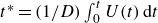
The actual kinematics were verified using two independent methods. First, a nine-axis offline accelerometer data logger (WT901SDCL) mounted on the linear guide was employed, and velocity and displacement profiles were obtained by integrating the recorded acceleration data. Second, a high-speed CMOS camera captured the positions of the plate and the L-shaped sting connection point (i.e. the centre of the circular plate) at various time instants, and differential analysis of these positions was conducted to derive the velocity. Each method was repeated 10 times to ensure reliability. A comparative analysis of the conformity between theoretical and actual velocity profiles under two distinct conditions,
 $ a^* = 0.25, Re = 4 \times 10^4$
and
$ a^* = 0.25, Re = 4 \times 10^4$
and
 $ a^* = 2.0, Re = 8 \times 10^4$
, is shown in figure 2. For measurements based on image data, displacement serves as the raw data, while velocity is derived through differentiation. However, acceleration is not further calculated by differentiation due to the typically unacceptable errors introduced by double differentiation, where Rick Chartrand’s algorithm for numerical differentiation of noisy data will be considered in future research (Chartrand Reference Chartrand2011). The uncertainty associated with the instantaneous velocity is 1.2 % for the accelerometer and 4.6 % for image acquisition under
$ a^* = 2.0, Re = 8 \times 10^4$
, is shown in figure 2. For measurements based on image data, displacement serves as the raw data, while velocity is derived through differentiation. However, acceleration is not further calculated by differentiation due to the typically unacceptable errors introduced by double differentiation, where Rick Chartrand’s algorithm for numerical differentiation of noisy data will be considered in future research (Chartrand Reference Chartrand2011). The uncertainty associated with the instantaneous velocity is 1.2 % for the accelerometer and 4.6 % for image acquisition under
 $ a^* = 0.25, Re = 4 \times 10^4$
, and 0.7 % and 5.3 %, respectively, under
$ a^* = 0.25, Re = 4 \times 10^4$
, and 0.7 % and 5.3 %, respectively, under
 $ a^* = 1.0, Re = 8 \times 10^4$
during the constant velocity stage. The larger error in the image-based measurements is attributed to more pronounced oscillations of the plate mounted at the bottom. In contrast, the accelerometer, mounted on the linear guider (as shown in figure 1), is unaffected by oscillations of the cantilever beam caused by the L-shaped sting.
$ a^* = 1.0, Re = 8 \times 10^4$
during the constant velocity stage. The larger error in the image-based measurements is attributed to more pronounced oscillations of the plate mounted at the bottom. In contrast, the accelerometer, mounted on the linear guider (as shown in figure 1), is unaffected by oscillations of the cantilever beam caused by the L-shaped sting.
The kinematics validation under the conditions of
 $ a^* = 0.25, \, Re = 4 \times 10^4$
in (a–c) and
$ a^* = 0.25, \, Re = 4 \times 10^4$
in (a–c) and
 $ a^* = 1.0, \, Re = 8 \times 10^4$
in (d–f) is presented. The acceleration calibration is shown in (a) and (d), the velocity calibration in (b) and (e), and the displacement calibration in (c) and (f). The black dashed lines represent the theoretical values, the red solid lines are based on accelerometer data and the blue solid lines are based on image data.
$ a^* = 1.0, \, Re = 8 \times 10^4$
in (d–f) is presented. The acceleration calibration is shown in (a) and (d), the velocity calibration in (b) and (e), and the displacement calibration in (c) and (f). The black dashed lines represent the theoretical values, the red solid lines are based on accelerometer data and the blue solid lines are based on image data.

Polycarbonate sheets are utilized to fabricate plates with varying degrees of flexibility. These sheets have a density of
 $ \rho _m = 1.194 \times 10^3 \, \mathrm{kg\,m^{- 3}}$
, a Young’s modulus
$ \rho _m = 1.194 \times 10^3 \, \mathrm{kg\,m^{- 3}}$
, a Young’s modulus
 $ E = 2220 \, \mathrm{MPa}$
, and a Poisson’s ratio
$ E = 2220 \, \mathrm{MPa}$
, and a Poisson’s ratio
 $ \hat {\nu } = 0.370$
. The plates differ in thickness
$ \hat {\nu } = 0.370$
. The plates differ in thickness
 $ h$
, and assuming 1-D deformation of a beam-type plate, the bending stiffness is calculated using the formula (Landau et al. Reference Landau, Pitaevskii, Kosevich and Lifshitz2012)
$ h$
, and assuming 1-D deformation of a beam-type plate, the bending stiffness is calculated using the formula (Landau et al. Reference Landau, Pitaevskii, Kosevich and Lifshitz2012)
 \begin{equation} \textit{EI} = \frac {E h^3}{12 (1 - \hat {\nu }^2)}. \end{equation}
The flexibility parameters are summarized in table 2. An uncertainty analysis for the bending stiffness,
 ${\textit{EI}}$
, was conducted. The uncertainty arises primarily from Young’s Modulus (
${\textit{EI}}$
, was conducted. The uncertainty arises primarily from Young’s Modulus (
 $E$
) and plate thickness (
$E$
) and plate thickness (
 $h$
) (2.2). A conservative relative uncertainty of
$h$
) (2.2). A conservative relative uncertainty of
 $\sigma _E / E = 5.0\,\%$
was adopted for
$\sigma _E / E = 5.0\,\%$
was adopted for
 $E$
to account for batch-to-batch variations in the commercial-grade polycarbonate (Callister & Rethwisch Reference Callister and Rethwisch1999). To quantify thickness variability, each plate was measured at 16 points in a radial and azimuthal pattern using a thickness gauge (SANLIANG 325-308, 0.001 mm resolution). The results (table 2) show excellent material uniformity, with thickness variability (
$E$
to account for batch-to-batch variations in the commercial-grade polycarbonate (Callister & Rethwisch Reference Callister and Rethwisch1999). To quantify thickness variability, each plate was measured at 16 points in a radial and azimuthal pattern using a thickness gauge (SANLIANG 325-308, 0.001 mm resolution). The results (table 2) show excellent material uniformity, with thickness variability (
 $\sigma _h / h_{\textit{avg}}$
) below 2 %. Subsequent calculations used the measured mean thickness,
$\sigma _h / h_{\textit{avg}}$
) below 2 %. Subsequent calculations used the measured mean thickness,
 $h_{\textit{avg}}$
, for improved accuracy. The total relative uncertainty in
$h_{\textit{avg}}$
, for improved accuracy. The total relative uncertainty in
 ${\textit{EI}}$
was estimated via error propagation (Taylor Reference Taylor2022):
${\textit{EI}}$
was estimated via error propagation (Taylor Reference Taylor2022):
 \begin{equation} \left (\frac {\sigma _{\textit{EI}}}{\textit{EI}}\right )^2 \approx \left (\frac {\sigma _E}{E}\right )^2 + \left (3 \frac {\sigma _h}{h_{\textit{avg}}}\right )^2. \end{equation}
This yields a maximum uncertainty of approximately 7.1 % for the thinnest plate, which has the largest thickness variability (1.7 %). The uncertainty from Young’s modulus (5.0 %) is a primary contributor, being comparable to or greater than the contribution from thickness (
 $0.23\,\% \leqslant 3\sigma _h/h_{\textit{avg}} \leqslant 5.1\,\%$
). Henceforth, plates are referred to by their nominal thickness,
$0.23\,\% \leqslant 3\sigma _h/h_{\textit{avg}} \leqslant 5.1\,\%$
). Henceforth, plates are referred to by their nominal thickness,
 $h_{\textit{nom}}$
(e.g. ‘the 0.30 mm plate’), for brevity. All calculations, however, use the measured mean thickness,
$h_{\textit{nom}}$
(e.g. ‘the 0.30 mm plate’), for brevity. All calculations, however, use the measured mean thickness,
 $h_{\textit{avg}}$
, from table 2.
$h_{\textit{avg}}$
, from table 2.
Flexibility parameters of the polycarbonate plates. Here
 $h_{\textit{nom}}$
is the nominal thickness, while the mean thickness (
$h_{\textit{nom}}$
is the nominal thickness, while the mean thickness (
 $h_{\textit{avg}}$
) and its relative variability (
$h_{\textit{avg}}$
) and its relative variability (
 $\sigma _h/h_{\textit{avg}}$
) were determined from 16-point measurements. The bending stiffness (
$\sigma _h/h_{\textit{avg}}$
) were determined from 16-point measurements. The bending stiffness (
 ${\textit{EI}}$
) was calculated using the measured
${\textit{EI}}$
) was calculated using the measured
 $h_{\textit{avg}}$
. The total relative uncertainty shown in the final column,
$h_{\textit{avg}}$
. The total relative uncertainty shown in the final column,
 $\sigma _{\textit{EI}}/EI$
, results from propagating the uncertainties from two sources: the estimated uncertainty in Young’s Modulus and the measured variability in thickness, as detailed in (2.3).
$\sigma _{\textit{EI}}/EI$
, results from propagating the uncertainties from two sources: the estimated uncertainty in Young’s Modulus and the measured variability in thickness, as detailed in (2.3).

The flexible plate undergoes deformation due to its inability to resist the hydrodynamic forces during translation. To track this deformation, the chordwise plane crossing the centre of the circular plate was illuminated by the laser sheet. The deformation was recorded using the high-speed CMOS camera. A threshold-based image segmentation method (Suzuki et al. Reference Suzuki1985) was employed to extract the plate deformation. Due to the deformation, the projected area of the plate is given by
 \begin{equation} S_p = 2 \int _0^{D/2} 2 \sqrt {\left (\frac {D}{2}\right )^2 - l^2} \cos \theta \, \mathrm{d}l, \end{equation}
where
 $ l$
is the curvilinear coordinate along the radius from the centre towards the tip in the chordwise plane and can be expressed as
$ l$
is the curvilinear coordinate along the radius from the centre towards the tip in the chordwise plane and can be expressed as
 \begin{equation} l = \int _0^l \mathrm{d}l = \int _0^z \frac {\mathrm{d}l}{\mathrm{d}z} \mathrm{d}z = \int _0^z \sqrt {k^2 + 1} \, \mathrm{d}z, \end{equation}
and
 $ \theta$
is the angle between the plate and the vertical
$ \theta$
is the angle between the plate and the vertical
 $z$
axis. The cosine of the angle is defined as
$z$
axis. The cosine of the angle is defined as
 \begin{equation} \cos \theta = \frac {1}{\sqrt {k^2 + 1}}, \end{equation}
where
 $ k$
is the slope of the curvilinear line. The dimensionless projected area is defined as
$ k$
is the slope of the curvilinear line. The dimensionless projected area is defined as
 \begin{equation} S_p^* = \frac {S_p}{S}, \end{equation}
where
 $S = \pi D^2/4$
is considered the wetted area of the plate.
$S = \pi D^2/4$
is considered the wetted area of the plate.
Furthermore, the velocities of the plate centre
 $U_{{\textit{centre}}}$
and tip
$U_{{\textit{centre}}}$
and tip
 $U_{{\textit{tip}}}$
can be determined based on the displacement differences of the corresponding points at successive time frames.
$U_{{\textit{tip}}}$
can be determined based on the displacement differences of the corresponding points at successive time frames.
Shape tracing and kinematics of the flexible plate (
 $h_{\textit{nom}}=0.30\,\mathrm{mm}$
) for
$h_{\textit{nom}}=0.30\,\mathrm{mm}$
) for
 $a^*=0.25$
(
$a^*=0.25$
(
 $t_a^*=2.0$
) and
$t_a^*=2.0$
) and
 ${\textit{Re}}=7\times 10^4$
. (a,c) Raw images of the plate deformation in the chordwise and spanwise planes, respectively. In these images, the thick bright line is the plate’s centreline directly illuminated by the laser, while the thinner lines are the illuminated contours of the plate. The non-smooth appearance of the contour is an artefact of the multi-sub-FOV method used for image acquisition (§ 2.4), but it does not affect the accurate extraction of the centreline profile. (b,d) Corresponding traced profiles, showing a C-shaped deformation chordwise while the spanwise profile remains straight. (e) Evolution of the dimensionless projected area,
${\textit{Re}}=7\times 10^4$
. (a,c) Raw images of the plate deformation in the chordwise and spanwise planes, respectively. In these images, the thick bright line is the plate’s centreline directly illuminated by the laser, while the thinner lines are the illuminated contours of the plate. The non-smooth appearance of the contour is an artefact of the multi-sub-FOV method used for image acquisition (§ 2.4), but it does not affect the accurate extraction of the centreline profile. (b,d) Corresponding traced profiles, showing a C-shaped deformation chordwise while the spanwise profile remains straight. (e) Evolution of the dimensionless projected area,
 $S_p^*$
, with formation time. (f) Instantaneous velocities of the plate centre (
$S_p^*$
, with formation time. (f) Instantaneous velocities of the plate centre (
 $U_{{\textit{centre}}}$
) and tip (
$U_{{\textit{centre}}}$
) and tip (
 $U_{{\textit{tip}}}$
).
$U_{{\textit{tip}}}$
).

As a representative example, figure 3 shows the deformation of a flexible plate (
 $h_{\textit{nom}}=0.30\,\mathrm{mm}$
at
$h_{\textit{nom}}=0.30\,\mathrm{mm}$
at
 $a^* = 0.25$
and
$a^* = 0.25$
and
 ${\textit{Re}} = 7 \times 10^4$
). The plate exhibits a symmetric, C-shaped bending profile in the chordwise direction (figure 3
a), which contrasts with the multifold patterns reported by Schouveiler & Eloy (Reference Schouveiler and Eloy2013). This confirms that the central support constrains deformation to the intended beam-like mode (§ 2.1). The quantified profiles further show a clear C-shape chordwise while the spanwise section remains straight, confirming the suppression of multifold deformation (figure 3
b,d). Based on the traced geometries, the dimensionless projected area
${\textit{Re}} = 7 \times 10^4$
). The plate exhibits a symmetric, C-shaped bending profile in the chordwise direction (figure 3
a), which contrasts with the multifold patterns reported by Schouveiler & Eloy (Reference Schouveiler and Eloy2013). This confirms that the central support constrains deformation to the intended beam-like mode (§ 2.1). The quantified profiles further show a clear C-shape chordwise while the spanwise section remains straight, confirming the suppression of multifold deformation (figure 3
b,d). Based on the traced geometries, the dimensionless projected area
 $ S_p^*$
(figure 3
e), as well as the velocities of the plate centre and tip (figure 3
f), are calculated. To assess the run-to-run variability of the deformation, the shape tracking experiment was repeated five times. For this representative case, the run-to-run relative standard deviation of the projected area (
$ S_p^*$
(figure 3
e), as well as the velocities of the plate centre and tip (figure 3
f), are calculated. To assess the run-to-run variability of the deformation, the shape tracking experiment was repeated five times. For this representative case, the run-to-run relative standard deviation of the projected area (
 $S_p^*$
) is less than
$S_p^*$
) is less than
 $0.01\,\%$
, while for the centre and tip velocities it is
$0.01\,\%$
, while for the centre and tip velocities it is
 $0.8\,\%$
and
$0.8\,\%$
and
 $1.9\,\%$
, respectively. The low variability in
$1.9\,\%$
, respectively. The low variability in
 $S_p^*$
is expected, as its integral calculation smooths noise from the position data. Conversely, the higher velocity variability results from numerical differentiation, which is known to amplify noise. The slightly greater variation at the tip is attributed to its unconstrained free-end condition. These low deviations confirm the high repeatability of the measurements. Across all cases considered (table 3), the maximum relative standard deviation for
$S_p^*$
is expected, as its integral calculation smooths noise from the position data. Conversely, the higher velocity variability results from numerical differentiation, which is known to amplify noise. The slightly greater variation at the tip is attributed to its unconstrained free-end condition. These low deviations confirm the high repeatability of the measurements. Across all cases considered (table 3), the maximum relative standard deviation for
 $S_p^*$
did not exceed 0.13 %. This quantitative evidence of low standard deviation confirms that the plate’s motion is repeatable, dominated by large-scale fluid–structure reconfiguration rather than random vibrations.
$S_p^*$
did not exceed 0.13 %. This quantitative evidence of low standard deviation confirms that the plate’s motion is repeatable, dominated by large-scale fluid–structure reconfiguration rather than random vibrations.
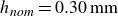
Nomenclature used in the study. ‘R-’ denotes rigid plates with
 ${\textit{EI}}^* = 2.66 \times 10^{-1}$
, ‘F-’ represents flexible plates with
${\textit{EI}}^* = 2.66 \times 10^{-1}$
, ‘F-’ represents flexible plates with
 ${\textit{EI}}^* = 1.16 \times 10^{-2}$
and ‘EF-’ indicates extra-flexible plates with
${\textit{EI}}^* = 1.16 \times 10^{-2}$
and ‘EF-’ indicates extra-flexible plates with
 ${\textit{EI}}^* = 1.19 \times 10^{-2}$
. The number following each letter specifies the corresponding Reynolds number. All cases were conducted under the conditions of
${\textit{EI}}^* = 1.19 \times 10^{-2}$
. The number following each letter specifies the corresponding Reynolds number. All cases were conducted under the conditions of
 $a^*=0.25$
(
$a^*=0.25$
(
 $t_{a}^*=2.0$
).
$t_{a}^*=2.0$
).
2.3. Force data acquisition
The hydrodynamic force measurement scheme was adapted from the work of Reynolds et al. (Reference Reynolds, Thomas and Taylor2014), Grift et al. (Reference Grift, Vijayaragavan, Tummers and Westerweel2019) and Fernando & Rival (Reference Fernando and Rival2016a
). A force/torque transducer (ATI Gamma F/T Mux SI-130-10) was installed between the linear guide and the L-shaped sting, as shown in figure 1. The Gamma F/T Mux force transducer has a force range of
 $\pm 130$
N with a resolution of 0.025 N. Data were recorded at a sampling frequency of 7000 Hz in this study. Under static conditions, the natural frequency of the system was approximately
$\pm 130$
N with a resolution of 0.025 N. Data were recorded at a sampling frequency of 7000 Hz in this study. Under static conditions, the natural frequency of the system was approximately
 $48.7 \pm 3.3$
Hz in air and
$48.7 \pm 3.3$
Hz in air and
 $46.7\pm 3.3$
Hz in water. Under dynamic conditions as listed in table 1, the natural frequency was approximately
$46.7\pm 3.3$
Hz in water. Under dynamic conditions as listed in table 1, the natural frequency was approximately
 $50.3 \pm 1.4$
Hz in air and
$50.3 \pm 1.4$
Hz in air and
 $48.0 \pm 1.1$
Hz in water. Based on the kinematics of the plate in this study as mentioned in § 2.2, the time interval corresponding to the plate’s acceleration is
$48.0 \pm 1.1$
Hz in water. Based on the kinematics of the plate in this study as mentioned in § 2.2, the time interval corresponding to the plate’s acceleration is
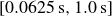 $[0.0625\, \mathrm{s} , 1.0\, \mathrm{s} ]$
or
$[0.0625\, \mathrm{s} , 1.0\, \mathrm{s} ]$
or
 $[1\, \mathrm{Hz} , 16\, \mathrm{Hz}]$
, different from the natural frequency to avoid resonance. A low-pass filter with a 40 Hz cutoff frequency was first applied to remove high-frequency noise. Subsequently, a second-order Savitzky–Golay filter (Savitzky & Golay Reference Savitzky and Golay1964) with a filter window width of
$[1\, \mathrm{Hz} , 16\, \mathrm{Hz}]$
, different from the natural frequency to avoid resonance. A low-pass filter with a 40 Hz cutoff frequency was first applied to remove high-frequency noise. Subsequently, a second-order Savitzky–Golay filter (Savitzky & Golay Reference Savitzky and Golay1964) with a filter window width of
 $\Delta t^* = 0.1$
was used to reduce noise. This window corresponds to an absolute time range of
$\Delta t^* = 0.1$
was used to reduce noise. This window corresponds to an absolute time range of
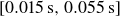 $[0.015\, \mathrm{s}, 0.055\, \mathrm{s}]$
, allowing for 6–20 filter windows during the acceleration phase to retain as much instantaneous force information as possible. The sensitivity of the filter window is quantified in Appendix A2.
$[0.015\, \mathrm{s}, 0.055\, \mathrm{s}]$
, allowing for 6–20 filter windows during the acceleration phase to retain as much instantaneous force information as possible. The sensitivity of the filter window is quantified in Appendix A2.
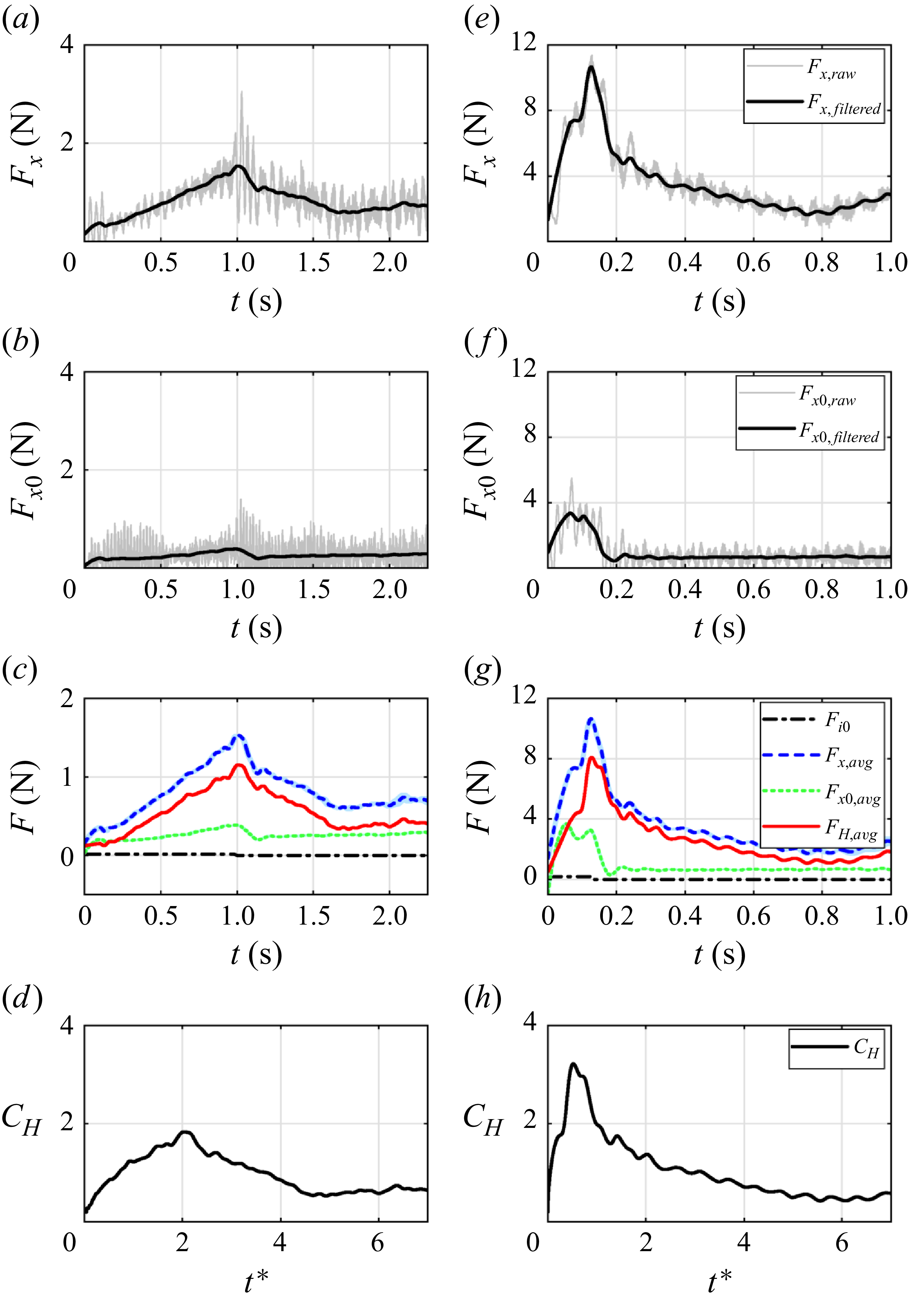
Force data acquisition for a 3.00 mm-thick plate was conducted under the conditions of
 $ a^* = 0.25$
(
$ a^* = 0.25$
(
 $t_a^*=2.0$
),
$t_a^*=2.0$
),
 ${\textit{Re}} = 4 \times 10^4$
in panels (a–d), and under the conditions of
${\textit{Re}} = 4 \times 10^4$
in panels (a–d), and under the conditions of
 $ a^* = 1.0$
(
$ a^* = 1.0$
(
 $t_a^*=0.5$
),
$t_a^*=0.5$
),
 ${\textit{Re}} = 8 \times 10^4$
in panels (e–h). Panels (a) and (e) illustrate the raw force
${\textit{Re}} = 8 \times 10^4$
in panels (e–h). Panels (a) and (e) illustrate the raw force
 $ F_{x,{raw}}$
(grey thin solid lines) obtained from a single measurement on the plate, along with its filtered results
$ F_{x,{raw}}$
(grey thin solid lines) obtained from a single measurement on the plate, along with its filtered results
 $ F_{x,{filtered}}$
(black thin solid lines) as a function of time
$ F_{x,{filtered}}$
(black thin solid lines) as a function of time
 $ t$
. The force measurements without the plate are depicted in panels (b) and (f). The relative standard deviations of
$ t$
. The force measurements without the plate are depicted in panels (b) and (f). The relative standard deviations of
 $ F_{x,{avg}}$
and
$ F_{x,{avg}}$
and
 $ F_{x0,{avg}}$
are 1.0 % and 1.3 %, respectively, relative to the maximum value in panel (c), and 0.9 % and 0.4 % in panel (g) over 10 measurements, indicating excellent repeatability of the data. The resultant hydrodynamic forces
$ F_{x0,{avg}}$
are 1.0 % and 1.3 %, respectively, relative to the maximum value in panel (c), and 0.9 % and 0.4 % in panel (g) over 10 measurements, indicating excellent repeatability of the data. The resultant hydrodynamic forces
 $ F_H$
(red solid line) in panels (c) and (g) are obtained by subtracting
$ F_H$
(red solid line) in panels (c) and (g) are obtained by subtracting
 $ F_{x,{avg}}$
(blue dashed line) from
$ F_{x,{avg}}$
(blue dashed line) from
 $ F_{x0,{avg}}$
(green dotted line) and the inertial force
$ F_{x0,{avg}}$
(green dotted line) and the inertial force
 $ F_{i_0}$
(black dashed–dotted line, accounts for less than 0.1 % of
$ F_{i_0}$
(black dashed–dotted line, accounts for less than 0.1 % of
 $ F_H$
) in both panels (c) and (g). Lastly, the hydrodynamic force coefficients
$ F_H$
) in both panels (c) and (g). Lastly, the hydrodynamic force coefficients
 $ C_H$
are plotted against the dimensionless time
$ C_H$
are plotted against the dimensionless time
 $ t^*$
in panels (d) and (h).
$ t^*$
in panels (d) and (h).
In actual measurements, the force with the plate attached in the
 $x$
-direction
$x$
-direction
 $F_x$
was first measured and filtered as exemplified in figure 4(a,e). Subsequently, the force without the flexible plate in the
$F_x$
was first measured and filtered as exemplified in figure 4(a,e). Subsequently, the force without the flexible plate in the
 $x$
-direction
$x$
-direction
 $F_{x0}$
was measured and filtered as shown in figure 4(b,f). Considering the inertial force
$F_{x0}$
was measured and filtered as shown in figure 4(b,f). Considering the inertial force
 $F_i(t)$
due to the acceleration of the plate itself, the hydrodynamic force can be expressed as
$F_i(t)$
due to the acceleration of the plate itself, the hydrodynamic force can be expressed as
 \begin{equation} F_H(t) = F_x(t) - F_{x0}(t) - F_i(t), \end{equation}
where, due to the bending deformation, the acceleration at different parts of the plate varies. Specifically, since the flexible deformation is directed backwards, during the acceleration phase, the acceleration of each part of the plate is less than that of the plate centre, i.e.
 $\partial U_i / \partial t \leqslant a$
. Therefore, the actual inertial force of the flexible plate is less than its inertial force in the undeformed state, i.e.
$\partial U_i / \partial t \leqslant a$
. Therefore, the actual inertial force of the flexible plate is less than its inertial force in the undeformed state, i.e.
 \begin{equation} F_i(t) = 2 \sum _{i=0}^{N} m_i \frac {\partial U_i}{\partial t} \leqslant F_{i0}(t) = 2 \sum _{i=0}^{N} m_i a(t) = \rho _m S h a(t), \end{equation}
where, the deformation of different segments with mass
 $ m_i$
of the plate was obtained, allowing us to determine the displacement
$ m_i$
of the plate was obtained, allowing us to determine the displacement
 $ x_i$
, velocity
$ x_i$
, velocity
 $ U_i$
and acceleration
$ U_i$
and acceleration
 $ \partial U_i/\partial t$
for each segment;
$ \partial U_i/\partial t$
for each segment;
 $i=0$
is the segment through the centre of the plate and
$i=0$
is the segment through the centre of the plate and
 $i=N$
is the segment of the tip of the plate. As shown in figure 4(c,g),
$i=N$
is the segment of the tip of the plate. As shown in figure 4(c,g),
 $F_{i0}(t)$
accounts for less than 0.1 % of the hydrodynamic force. Thus,
$F_{i0}(t)$
accounts for less than 0.1 % of the hydrodynamic force. Thus,
 $F_{i0}(t)$
can be neglected and the calculation of
$F_{i0}(t)$
can be neglected and the calculation of
 $F_H(t)$
can be approximated as
$F_H(t)$
can be approximated as
 \begin{equation} F_H(t) \approx F_x(t) - F_{x0}(t). \end{equation}
The resulting hydrodynamic force is shown in figure 4(c,g). All data sets were averaged over 10 runs. The relative standard deviation of the hydrodynamic force for each plate is less than 1.3 %. Based on the hydrodynamic force, the classical hydrodynamic force coefficient is defined as
 \begin{equation} C_H = \frac {F_H}{\dfrac {1}{2} \rho _{\!f} U_c^2 S}. \end{equation}
The resulting force coefficient
 $C_H$
is shown in figure 4(d,h). The uncertainty in the hydrodynamic force coefficient,
$C_H$
is shown in figure 4(d,h). The uncertainty in the hydrodynamic force coefficient,
 $C_H$
, was quantified using error propagation. The worst-case scenario was selected based on the physical acceleration (
$C_H$
, was quantified using error propagation. The worst-case scenario was selected based on the physical acceleration (
 $a = a^* U_c^2 / D$
), which is the primary driver of vibrational noise in the measurements. The high-acceleration kinematics validation case (
$a = a^* U_c^2 / D$
), which is the primary driver of vibrational noise in the measurements. The high-acceleration kinematics validation case (
 $a^*=1.0, Re=8 \times 10^4$
), with
$a^*=1.0, Re=8 \times 10^4$
), with
 $a \approx 6.43\,{\rm m\,s}^{-2}$
, was therefore chosen as the most conservative benchmark. Assuming uncorrelated errors, the uncertainty in
$a \approx 6.43\,{\rm m\,s}^{-2}$
, was therefore chosen as the most conservative benchmark. Assuming uncorrelated errors, the uncertainty in
 $C_H$
is propagated from the standard deviations of the measured forces (
$C_H$
is propagated from the standard deviations of the measured forces (
 $\sigma _{F_x}$
and
$\sigma _{F_x}$
and
 $\sigma _{F_{x0}}$
) as
$\sigma _{F_{x0}}$
) as
 \begin{equation} \sigma _{C_H} = \frac {\sqrt {\sigma _{F_x}^2 + \sigma _{F_{x0}}^2}}{\dfrac {1}{2}\rho _{\!f} U_c^2 S}. \end{equation}
Using data from this high-acceleration benchmark case (figure 4), the propagated uncertainty was estimated to be approximately 2.9 %, which confirms the high precision of the force measurements.
Further, the instantaneous force coefficient normalized by the projected area can be defined as
 \begin{equation} C_H^* = \frac {C_H}{S_p^*}. \end{equation}
The
 $C_H$
of the 3.00 mm-thick plate at
$C_H$
of the 3.00 mm-thick plate at
 $a^* = 0.50$
,
$a^* = 0.50$
,
 $1.0$
and
$1.0$
and
 $2.0$
, and
$2.0$
, and
 ${\textit{Re}} = 8 \times 10^4$
was used to compare with results from the previous literature, as shown in figure 5. Within
${\textit{Re}} = 8 \times 10^4$
was used to compare with results from the previous literature, as shown in figure 5. Within
 $t^* \in [0,7]$
, the deviation between the force measurement results of this study and Li et al. (Reference Li, Xiang, Qin, Liu and Wang2022) is 1.1 %, and Fernando et al. (Reference Fernando, Weymouth and Rival2020) is 4.6 %.
$t^* \in [0,7]$
, the deviation between the force measurement results of this study and Li et al. (Reference Li, Xiang, Qin, Liu and Wang2022) is 1.1 %, and Fernando et al. (Reference Fernando, Weymouth and Rival2020) is 4.6 %.
The force data acquisition was validated by comparing the results with previously published data for a rigid plate (
 $h_{\textit{nom}}=3.00 \, \mathrm{mm}$
): (a)
$h_{\textit{nom}}=3.00 \, \mathrm{mm}$
): (a)
 $a^* = 0.5$
(
$a^* = 0.5$
(
 $t_a^*=1.0$
),
$t_a^*=1.0$
),
 ${\textit{Re}}=8\times 10^4$
; (b)
${\textit{Re}}=8\times 10^4$
; (b)
 $a^* = 1.0$
(
$a^* = 1.0$
(
 $t_a^*=0.5$
),
$t_a^*=0.5$
),
 ${\textit{Re}}=8\times 10^4$
; (c)
${\textit{Re}}=8\times 10^4$
; (c)
 $a^* = 2.0$
(
$a^* = 2.0$
(
 $t_a^*=0.25$
),
$t_a^*=0.25$
),
 ${\textit{Re}}=8\times 10^4$
. The green solid lines are adopted from the Fernando et al. (Reference Fernando, Weymouth and Rival2020), blue solid lines are adopted from Li et al. (Reference Li, Xiang, Qin, Liu and Wang2022) and the red solid lines are the force coefficient measured by current set-up. It is important to note that the definition of the drag coefficient in Fernando et al. (Reference Fernando, Weymouth and Rival2020) differs from the definition of the hydrodynamic coefficient used in this study by a factor of
${\textit{Re}}=8\times 10^4$
. The green solid lines are adopted from the Fernando et al. (Reference Fernando, Weymouth and Rival2020), blue solid lines are adopted from Li et al. (Reference Li, Xiang, Qin, Liu and Wang2022) and the red solid lines are the force coefficient measured by current set-up. It is important to note that the definition of the drag coefficient in Fernando et al. (Reference Fernando, Weymouth and Rival2020) differs from the definition of the hydrodynamic coefficient used in this study by a factor of
 $\pi /8$
, and to ensure a fair comparison, the data from Fernando et al. (Reference Fernando, Weymouth and Rival2020) have been adjusted accordingly.
$\pi /8$
, and to ensure a fair comparison, the data from Fernando et al. (Reference Fernando, Weymouth and Rival2020) have been adjusted accordingly.

2.4. Flow field measurement
Two-dimensional, two-velocity-component (2D2C) time-resolved planar PIV was employed to quantitatively capture the flow fields. The 2D2C PIV configuration was deemed sufficient for this study’s primary goal: to uncover the physical mechanisms behind the load-shifting phenomenon. While vortex rings are inherently three-dimensional (3-D), a multislice measurement strategy was implemented to capture the critical wake features. This planar approach is directly compatible with the vorticity moment theorem used for force estimation, which requires only 2-D velocity and vorticity data (§ 5.1).
Multislice measurements were conducted in three representative cross-sectional planes relative to the plate: the chordwise (
 $\theta = 0^\circ$
), diagonal (
$\theta = 0^\circ$
), diagonal (
 $\theta = 45^\circ$
) and spanwise (
$\theta = 45^\circ$
) and spanwise (
 $\theta = 90^\circ$
) sections. In each case, the laser sheet was projected from the left-hand side of the water tank across the plate’s centre, as illustrated in figure 1. A high-speed CMOS camera (Phantom VEO-640) positioned perpendicular to the laser sheet recorded the particle field images. To capture the flow fields of different cross-sections, the plate’s orientation was altered while the laser and camera positions remained fixed. This was accomplished using three separate horizontal rods, each fabricated with a mounting slot milled at a distinct angle (
$\theta = 90^\circ$
) sections. In each case, the laser sheet was projected from the left-hand side of the water tank across the plate’s centre, as illustrated in figure 1. A high-speed CMOS camera (Phantom VEO-640) positioned perpendicular to the laser sheet recorded the particle field images. To capture the flow fields of different cross-sections, the plate’s orientation was altered while the laser and camera positions remained fixed. This was accomplished using three separate horizontal rods, each fabricated with a mounting slot milled at a distinct angle (
 $0^\circ$
,
$0^\circ$
,
 $45^\circ$
or
$45^\circ$
or
 $90^\circ$
). Appendix A3 validates its effectiveness for consistently characterizing the different cross-sections of the wake. Hollow glass beads (spherical, density
$90^\circ$
). Appendix A3 validates its effectiveness for consistently characterizing the different cross-sections of the wake. Hollow glass beads (spherical, density
 $\rho _g = 1.03$
–
$\rho _g = 1.03$
–
 $1.05$
g cm−
$1.05$
g cm−
 $^3$
, diameter
$^3$
, diameter
 $d_g = 20$
–
$d_g = 20$
–
 $60 \, {\unicode{x03BC}} \mathrm{m}$
) served as tracer particles, illuminated by a double-pulsed 527 nm Nd-YLF laser (Beamtech Vlite-Hi-527,
$60 \, {\unicode{x03BC}} \mathrm{m}$
) served as tracer particles, illuminated by a double-pulsed 527 nm Nd-YLF laser (Beamtech Vlite-Hi-527,
 $\geqslant$
30 mJ at 1 kHz).
$\geqslant$
30 mJ at 1 kHz).
To maximize spatial resolution, theoretically, the FOV of over
 $7D$
was divided into three sub-FOVs along the
$7D$
was divided into three sub-FOVs along the
 $x$
-axis: sub-FOV1 (
$x$
-axis: sub-FOV1 (
 $-1D$
to
$-1D$
to
 $2D$
), sub-FOV2 (
$2D$
), sub-FOV2 (
 $2D$
to
$2D$
to
 $5D$
) and sub-FOV3 (
$5D$
) and sub-FOV3 (
 $5D$
to
$5D$
to
 $8D$
), where each sub-FOV was designed to have a theoretical size of
$8D$
), where each sub-FOV was designed to have a theoretical size of
 $3D \times 2D$
. The sub-FOVs were captured by fixing the camera and laser while altering the plate’s SP: SP1 for sub-FOV1, SP2 for sub-FOV2 and SP3 for sub-FOV3. Each sub-FOV was measured five times, with a 60 s interval between runs to avoid flow interference from prior tests. The distance between SP3 and the wall was
$3D \times 2D$
. The sub-FOVs were captured by fixing the camera and laser while altering the plate’s SP: SP1 for sub-FOV1, SP2 for sub-FOV2 and SP3 for sub-FOV3. Each sub-FOV was measured five times, with a 60 s interval between runs to avoid flow interference from prior tests. The distance between SP3 and the wall was
 $5D$
, sufficient to minimize wall effects. This distance was chosen also based on the laser beam waist, which was approximately 1 m from the laser head. As the deviation from this distance increases, the laser sheet thickness also increases, potentially introducing larger PIV errors. In this experiment, the distance between the centre of captured FOV to the laser head was 1.35 m, ensuring good imaging results while maintaining acceptable laser sheet thickness.
$5D$
, sufficient to minimize wall effects. This distance was chosen also based on the laser beam waist, which was approximately 1 m from the laser head. As the deviation from this distance increases, the laser sheet thickness also increases, potentially introducing larger PIV errors. In this experiment, the distance between the centre of captured FOV to the laser head was 1.35 m, ensuring good imaging results while maintaining acceptable laser sheet thickness.
In practice, each sub-FOV spanned
 $3.65D \times 2.28D$
by recorded with 2560
$3.65D \times 2.28D$
by recorded with 2560
 $\times$
1600 pixels (figure 1) and the adjacent windows overlapped and were stitched using interpolation (Li et al. Reference Li, Xiang, Qin, Liu and Wang2022). The sampling frequency for PIV data was 800 Hz, ensuring high temporal resolution. To ensure an optimal time delay (
$\times$
1600 pixels (figure 1) and the adjacent windows overlapped and were stitched using interpolation (Li et al. Reference Li, Xiang, Qin, Liu and Wang2022). The sampling frequency for PIV data was 800 Hz, ensuring high temporal resolution. To ensure an optimal time delay (
 $\Delta t$
) between frames, the maximum particle displacement was restricted to
$\Delta t$
) between frames, the maximum particle displacement was restricted to
 $0.25S_{{IS}}$
, where
$0.25S_{{IS}}$
, where
 $S_{{IS}}$
is the size of the interrogation spot. Using characteristic velocity
$S_{{IS}}$
is the size of the interrogation spot. Using characteristic velocity
 $U_c$
,
$U_c$
,
 $\Delta t$
was computed as
$\Delta t$
was computed as
 $\Delta t = 0.25 S_{{IS}}/2U_c$
, considering the maximum flow velocity magnitude to be approximately twice the plate’s translation velocity (Li et al. Reference Li, Xiang, Qin, Liu and Wang2022).
$\Delta t = 0.25 S_{{IS}}/2U_c$
, considering the maximum flow velocity magnitude to be approximately twice the plate’s translation velocity (Li et al. Reference Li, Xiang, Qin, Liu and Wang2022).
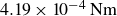
Effect of Reynolds number
 ${\textit{Re}}$
on transient force evolution for plates with
${\textit{Re}}$
on transient force evolution for plates with
 $a^*=0.25$
(
$a^*=0.25$
(
 $t_a^*=2.0$
) and varying bending stiffness: (a)
$t_a^*=2.0$
) and varying bending stiffness: (a)
 $h = 2.00 \, \mathrm{mm}, EI = 1.72\, \mathrm{Nm}$
; (b)
$h = 2.00 \, \mathrm{mm}, EI = 1.72\, \mathrm{Nm}$
; (b)
 $h = 0.30 \, \mathrm{mm}, EI = 5.79\times 10^{-3} \, \mathrm{Nm}$
; (c)
$h = 0.30 \, \mathrm{mm}, EI = 5.79\times 10^{-3} \, \mathrm{Nm}$
; (c)
 $h = 0.125 \, \mathrm{mm}, EI = 4.19\times 10^{-4} \, \mathrm{Nm}$
.
$h = 0.125 \, \mathrm{mm}, EI = 4.19\times 10^{-4} \, \mathrm{Nm}$
.

Image processing was performed using TSI Insight 4G software, following PIV analysis guidelines (Keane & Adrian Reference Keane and Adrian1989). Background subtraction and light intensity normalization (10
 $\times$
10 pixel window) were applied to mitigate measurement bias caused by particle brightness and laser intensity variations. The multipass method was applied with interrogation spot sizes of
$\times$
10 pixel window) were applied to mitigate measurement bias caused by particle brightness and laser intensity variations. The multipass method was applied with interrogation spot sizes of
 $64 \times 64$
pixels (initial pass) and
$64 \times 64$
pixels (initial pass) and
 $32 \times 32$
pixels (final pass), with a 50 % overlap. This yielded
$32 \times 32$
pixels (final pass), with a 50 % overlap. This yielded
 $159 \times 99$
velocity vectors per sub-FOV with a vector spacing of 2.31 mm. Vorticity fields were calculated using second-order finite differences on velocity data from eight neighbouring points.
$159 \times 99$
velocity vectors per sub-FOV with a vector spacing of 2.31 mm. Vorticity fields were calculated using second-order finite differences on velocity data from eight neighbouring points.
Uncertainty in flow measurements was estimated using the peak ratio method (Charonko & Vlachos Reference Charonko and Vlachos2013), incorporated in the Insight 4G software. This global method accounts for errors such as particle density, pixel displacement and preprocessing. For this study, velocity field uncertainty across all runs was less than 1.2 %.
To ensure statistical robustness, five independent runs were conducted for each representative case. The run-to-run variability of the derived flow metrics (discussed in §§ 4 and 5) proved to be minimal, with relative standard deviations for key integral quantities remaining below 4.9 %. Consequently,
 $\pm 1\sigma$
confidence intervals are included in the subsequent time-evolution plots to demonstrate the deterministic nature of the observed flow features. Furthermore, to calculate time derivatives for force estimation (§ 5), the same second-order Savitzky–Golay filter (
$\pm 1\sigma$
confidence intervals are included in the subsequent time-evolution plots to demonstrate the deterministic nature of the observed flow features. Furthermore, to calculate time derivatives for force estimation (§ 5), the same second-order Savitzky–Golay filter (
 $\Delta t^*=0.1$
, consistent with the force filter in Appendix A2) was applied to the PIV-derived time series.
$\Delta t^*=0.1$
, consistent with the force filter in Appendix A2) was applied to the PIV-derived time series.
3. Force
3.1.
Force evolution across different
 ${\textit{Re}}$
and
${\textit{EI}}$
${\textit{Re}}$
and
${\textit{EI}}$


The transient hydrodynamic force coefficients for circular plates with three orders of magnitude in bending stiffness,
 ${\textit{EI}} = 1.72\, \mathrm{Nm}$
,
${\textit{EI}} = 1.72\, \mathrm{Nm}$
,
 $5.79\times 10^{-3} \, \mathrm{Nm}$
and
$5.79\times 10^{-3} \, \mathrm{Nm}$
and
 $4.19\times 10^{-4} \, \mathrm{Nm}$
, under varying Reynolds numbers
$4.19\times 10^{-4} \, \mathrm{Nm}$
, under varying Reynolds numbers
 ${\textit{Re}}$
are shown in figure 6.
${\textit{Re}}$
are shown in figure 6.
For the plate with bending stiffness
 ${\textit{EI}} = 1.72\, \mathrm{Nm}$
(corresponding to a thickness of
${\textit{EI}} = 1.72\, \mathrm{Nm}$
(corresponding to a thickness of
 $h = 2.00 \, \mathrm{mm}$
), which behaves as a rigid plate with negligible deformation, the force curves collapse well across different Reynolds numbers, confirming a clear Reynolds number independence (Fernando & Rival Reference Fernando and Rival2016b
; Li et al. Reference Li, Xiang, Qin, Liu and Wang2022). Furthermore, the force evolution exhibits a distinct peak-and-valley pattern (figure 6
a). During acceleration, the force increases rapidly with
$h = 2.00 \, \mathrm{mm}$
), which behaves as a rigid plate with negligible deformation, the force curves collapse well across different Reynolds numbers, confirming a clear Reynolds number independence (Fernando & Rival Reference Fernando and Rival2016b
; Li et al. Reference Li, Xiang, Qin, Liu and Wang2022). Furthermore, the force evolution exhibits a distinct peak-and-valley pattern (figure 6
a). During acceleration, the force increases rapidly with
 $t^*$
, reaching a peak at
$t^*$
, reaching a peak at
 $t^* = 2$
, followed by a decrease to a minimum at
$t^* = 2$
, followed by a decrease to a minimum at
 $t^* \approx 5.5$
– the so-called ‘drag trough’ (Fernando & Rival Reference Fernando and Rival2016a
) – before rising again.
$t^* \approx 5.5$
– the so-called ‘drag trough’ (Fernando & Rival Reference Fernando and Rival2016a
) – before rising again.
As the bending stiffness decreases to
 ${\textit{EI}} = 5.79\times 10^{-3} \, \mathrm{Nm}$
(corresponding to a plate thickness of
${\textit{EI}} = 5.79\times 10^{-3} \, \mathrm{Nm}$
(corresponding to a plate thickness of
 $h = 0.30 \, \mathrm{mm}$
), the force response exhibits significant changes with increasing Reynolds number, leading to a breakdown of Reynolds number independence (figure 6
b). At
$h = 0.30 \, \mathrm{mm}$
), the force response exhibits significant changes with increasing Reynolds number, leading to a breakdown of Reynolds number independence (figure 6
b). At
 ${\textit{Re}} = 4 \times 10^4$
, the characteristic peak-and-valley pattern persists, with a distinct force peak at
${\textit{Re}} = 4 \times 10^4$
, the characteristic peak-and-valley pattern persists, with a distinct force peak at
 $t^* = 2$
and a trough at
$t^* = 2$
and a trough at
 $t^* \approx 5.5$
. However, compared with the rigid plate, the peak force is reduced, while the trough force is elevated. As
$t^* \approx 5.5$
. However, compared with the rigid plate, the peak force is reduced, while the trough force is elevated. As
 ${\textit{Re}}$
increases, the force peak gradually flattens, and the trough becomes less pronounced. At
${\textit{Re}}$
increases, the force peak gradually flattens, and the trough becomes less pronounced. At
 ${\textit{Re}} = 10 \times 10^4$
, the peak-and-valley pattern disappears entirely, resulting in a smooth and uniform force evolution with no discernible extrema. Notably, the force coefficient at
${\textit{Re}} = 10 \times 10^4$
, the peak-and-valley pattern disappears entirely, resulting in a smooth and uniform force evolution with no discernible extrema. Notably, the force coefficient at
 $t^* \approx 5.5$
initially increases with
$t^* \approx 5.5$
initially increases with
 ${\textit{Re}}$
before declining at higher values. These results indicate that, as the bending stiffness decreases, the unsteady force dynamics lose their Reynolds number independence, underscoring the coupled effects of flexibility and Reynolds number on force evolution.
${\textit{Re}}$
before declining at higher values. These results indicate that, as the bending stiffness decreases, the unsteady force dynamics lose their Reynolds number independence, underscoring the coupled effects of flexibility and Reynolds number on force evolution.
For plates with further reduced bending stiffness to
 ${\textit{EI}} = 4.19\times 10^{-4} \, \mathrm{Nm}$
(corresponding to a thickness of
${\textit{EI}} = 4.19\times 10^{-4} \, \mathrm{Nm}$
(corresponding to a thickness of
 $h = 0.125 \, \mathrm{mm}$
), the force curves remain non-collapsing across Reynolds numbers but exhibit consistent trends: a rapid rise during acceleration followed by stabilization with negligible fluctuations. The peak-and-valley pattern disappears entirely.
$h = 0.125 \, \mathrm{mm}$
), the force curves remain non-collapsing across Reynolds numbers but exhibit consistent trends: a rapid rise during acceleration followed by stabilization with negligible fluctuations. The peak-and-valley pattern disappears entirely.
Overall, these results emphasize the coupled effects of Reynolds number and flexibility on unsteady force dynamics, causing the force evolution on reconfigurable plates to deviate from the Reynolds number independence and peak-and-valley pattern observed in rigid plates.
3.2.
Non-dimensional bending stiffness
${\textit{EI}}^*$
independence of force evolution

The breakdown of Reynolds number scaling stems from its primary focus on fluid dynamics, whereas the reconfigurable plate in this study undergoes deformation that modifies the surrounding flow, resulting in a coupled fluid–structure interaction. To characterize this interaction, a non-dimensional bending stiffness,
 ${\textit{EI}}^*$
, is employed as
${\textit{EI}}^*$
, is employed as
 \begin{equation} {\textit{EI}}^* = \frac {\textit{EI}}{\rho _{\!f} U_c^2 D^3}. \end{equation}
The physical significance of
 ${\textit{EI}}^*$
has been interpreted differently across various studies. From an energy perspective, Schouveiler & Boudaoud (Reference Schouveiler and Boudaoud2006) defined the elastohydrodynamical number, expressed as
${\textit{EI}}^*$
has been interpreted differently across various studies. From an energy perspective, Schouveiler & Boudaoud (Reference Schouveiler and Boudaoud2006) defined the elastohydrodynamical number, expressed as
 $ 1/{\textit{EI}}^*$
, to represent the ratio of flow-induced potential energy to elastic bending energy. Similarly, Alben et al. (Reference Alben, Shelley and Zhang2002, Reference Alben, Shelley and Zhang2004) introduced a parameter equivalent to
$ 1/{\textit{EI}}^*$
, to represent the ratio of flow-induced potential energy to elastic bending energy. Similarly, Alben et al. (Reference Alben, Shelley and Zhang2002, Reference Alben, Shelley and Zhang2004) introduced a parameter equivalent to
 $ \sqrt {1/{\textit{EI}}^*}$
, balancing fluid kinetic energy with elastic potential energy. Alternatively, from a force perspective, De Langre (Reference De Langre2008) and Gosselin et al. (Reference Gosselin, De Langre and Machado-Almeida2010) considered the Cauchy number,
$ \sqrt {1/{\textit{EI}}^*}$
, balancing fluid kinetic energy with elastic potential energy. Alternatively, from a force perspective, De Langre (Reference De Langre2008) and Gosselin et al. (Reference Gosselin, De Langre and Machado-Almeida2010) considered the Cauchy number,
 $Ca$
, expressed as
$Ca$
, expressed as
 $ 1/{\textit{EI}}^*$
, as the ratio of fluid dynamic pressure to plate bending rigidity. In the present study,
$ 1/{\textit{EI}}^*$
, as the ratio of fluid dynamic pressure to plate bending rigidity. In the present study,
 ${\textit{EI}}^*$
is adopted from the perspective of wing flapping aerodynamics (Shyy et al. Reference Shyy, Aono, Chimakurthi, Trizila, Kang, Cesnik and Liu2010; Kang et al. Reference Kang, Aono, Cesnik and Shyy2011), characterizing the balance between elastic bending forces and aerodynamic forces. The derivation of
${\textit{EI}}^*$
is adopted from the perspective of wing flapping aerodynamics (Shyy et al. Reference Shyy, Aono, Chimakurthi, Trizila, Kang, Cesnik and Liu2010; Kang et al. Reference Kang, Aono, Cesnik and Shyy2011), characterizing the balance between elastic bending forces and aerodynamic forces. The derivation of
 ${\textit{EI}}^*$
can be found in the Supplementary material.
${\textit{EI}}^*$
can be found in the Supplementary material.
Three orders of magnitude of
 ${\textit{EI}}^*$
were selected as representative cases (table 3). The corresponding deformation and force data are shown in figure 7. From figure 7, despite variations in
${\textit{EI}}^*$
were selected as representative cases (table 3). The corresponding deformation and force data are shown in figure 7. From figure 7, despite variations in
 ${\textit{EI}}$
and
${\textit{EI}}$
and
 $ Re$
, the deformation (
$ Re$
, the deformation (
 $ S_p^*$
defined in (2.7)) and force evolution (
$ S_p^*$
defined in (2.7)) and force evolution (
 $ C_H$
defined in (2.11) and
$ C_H$
defined in (2.11) and
 $ C_H^*$
defined in (2.13)) collapse onto a single curve as a function of formation time, with only limited deviations under the same
$ C_H^*$
defined in (2.13)) collapse onto a single curve as a function of formation time, with only limited deviations under the same
 ${\textit{EI}}^*$
condition.
${\textit{EI}}^*$
condition.
The deformation behaviour under different
 ${\textit{EI}}^*$
values is presented in figure 7(a,b). For
${\textit{EI}}^*$
values is presented in figure 7(a,b). For
 ${\textit{EI}}^* = 2.66 \times 10^{-1}$
, no deformation is observed, and the plate maintains its projected area as a perfect circle, effectively behaving as rigid. At
${\textit{EI}}^* = 2.66 \times 10^{-1}$
, no deformation is observed, and the plate maintains its projected area as a perfect circle, effectively behaving as rigid. At
 ${\textit{EI}}^* = 1.16 \times 10^{-2}$
, moderate deformation occurs, categorizing the plate as flexible. For
${\textit{EI}}^* = 1.16 \times 10^{-2}$
, moderate deformation occurs, categorizing the plate as flexible. For
 ${\textit{EI}}^* = 1.19 \times 10^{-2}$
, significant deformation reduces the projected area to nearly half its original size, showing the plate as extra flexible.
${\textit{EI}}^* = 1.19 \times 10^{-2}$
, significant deformation reduces the projected area to nearly half its original size, showing the plate as extra flexible.
As for the force evolution, from figure 7(d,g), when
 ${\textit{EI}}^* = 2.66 \times 10^{-1}$
, the instantaneous force evolution follows the so called peak-and-valley pattern as discussed in § 3.1. When
${\textit{EI}}^* = 2.66 \times 10^{-1}$
, the instantaneous force evolution follows the so called peak-and-valley pattern as discussed in § 3.1. When
 ${\textit{EI}}^*$
decreases to
${\textit{EI}}^*$
decreases to
 $ 1.16 \times 10^{-2}$
(figure 7
e,h), the peak-and-valley characteristic weakens: the peak force decreases, the valley force increases and the force stabilizes around the steady drag coefficient after
$ 1.16 \times 10^{-2}$
(figure 7
e,h), the peak-and-valley characteristic weakens: the peak force decreases, the valley force increases and the force stabilizes around the steady drag coefficient after
 $ t^* \approx 4$
. Further reduction of
$ t^* \approx 4$
. Further reduction of
 ${\textit{EI}}^*$
to
${\textit{EI}}^*$
to
 $ 1.19 \times 10^{-2}$
eliminates the peak-valley pattern entirely (figure 7
f,i). The instantaneous force increases during the acceleration phase and stabilizes at
$ 1.19 \times 10^{-2}$
eliminates the peak-valley pattern entirely (figure 7
f,i). The instantaneous force increases during the acceleration phase and stabilizes at
 $ t^* \approx 1.5$
, earlier than the end of acceleration (
$ t^* \approx 1.5$
, earlier than the end of acceleration (
 $ t^* = 2$
). However, regardless of whether
$ t^* = 2$
). However, regardless of whether
 $ C_H$
or
$ C_H$
or
 $ C_H^*$
is considered, the instantaneous force coefficient curves collapse under identical
$ C_H^*$
is considered, the instantaneous force coefficient curves collapse under identical
 ${\textit{EI}}^*$
. This demonstrates that force evolution is primarily governed by
${\textit{EI}}^*$
. This demonstrates that force evolution is primarily governed by
 ${\textit{EI}}^*$
and remains consistent under the same non-dimensional bending stiffness conditions.
${\textit{EI}}^*$
and remains consistent under the same non-dimensional bending stiffness conditions.
Instantaneous
 $ S_p^*$
(a–c),
$ S_p^*$
(a–c),
 $ C_H$
(d–f) and
$ C_H$
(d–f) and
 $ C_H^*$
(g–i) for three orders of magnitude of
$ C_H^*$
(g–i) for three orders of magnitude of
 ${\textit{EI}}^*$
; legend details can be found in table 3.
${\textit{EI}}^*$
; legend details can be found in table 3.

3.3. Load-shifting phenomenon in force evolution
To further investigate the impact of different values of
 ${\textit{EI}}^*$
on the force evolution pattern, the reconfiguration number, originally defined under steady conditions by Gosselin et al. (Reference Gosselin, De Langre and Machado-Almeida2010), is extended to the unsteady accelerating process. The reconfiguration number
${\textit{EI}}^*$
on the force evolution pattern, the reconfiguration number, originally defined under steady conditions by Gosselin et al. (Reference Gosselin, De Langre and Machado-Almeida2010), is extended to the unsteady accelerating process. The reconfiguration number
 $ R(t^*)$
is defined as
$ R(t^*)$
is defined as
 \begin{equation} R(t^*) = \frac {C_{H_{\!f}}(t^*)}{C_{H_r}(t^*)}, \end{equation}
where
 $ C_{H_{\!f}}(t^*)$
and
$ C_{H_{\!f}}(t^*)$
and
 $ C_{H_r}(t^*)$
represent the instantaneous hydrodynamic force coefficients of the flexible/extra-flexible and rigid plates, respectively. This normalization employs the rigid response as a dynamic baseline, thereby removing the inherent time-dependent variations of the accelerating flow and isolating the effect of reconfiguration (Gosselin et al. Reference Gosselin, De Langre and Machado-Almeida2010). A value of
$ C_{H_r}(t^*)$
represent the instantaneous hydrodynamic force coefficients of the flexible/extra-flexible and rigid plates, respectively. This normalization employs the rigid response as a dynamic baseline, thereby removing the inherent time-dependent variations of the accelerating flow and isolating the effect of reconfiguration (Gosselin et al. Reference Gosselin, De Langre and Machado-Almeida2010). A value of
 $R(t^*) \lt 1$
indicates force reduction relative to the rigid case, and
$R(t^*) \lt 1$
indicates force reduction relative to the rigid case, and
 $R(t^*) \gt 1$
indicates enhancement.
$R(t^*) \gt 1$
indicates enhancement.
The reconfiguration number
 $ R$
and the absolute hydrodynamic force coefficient difference
$ R$
and the absolute hydrodynamic force coefficient difference
 $ \Delta C_H$
for the flexible plate (a,b) and extra-flexible plate (c,d). Legend details can be found in table 3.
$ \Delta C_H$
for the flexible plate (a,b) and extra-flexible plate (c,d). Legend details can be found in table 3.

Additionally, to clearly present the results, the absolute hydrodynamic force coefficient difference
 $ \Delta C_H$
is defined as
$ \Delta C_H$
is defined as
 \begin{equation} \Delta C_H(t^*) = C_{H_{\!f}}(t^*) - C_{H_r}(t^*). \end{equation}
A negative value (
 $\Delta C_H \lt 0$
) indicates force reduction, whereas a positive value (
$\Delta C_H \lt 0$
) indicates force reduction, whereas a positive value (
 $\Delta C_H \gt 0$
) represents force enhancement. While
$\Delta C_H \gt 0$
) represents force enhancement. While
 $R(t^*)$
is ideal for assessing the relative impact of reconfiguration,
$R(t^*)$
is ideal for assessing the relative impact of reconfiguration,
 $\Delta C_H(t^*)$
provides a direct measure of the force changes.
$\Delta C_H(t^*)$
provides a direct measure of the force changes.
Results for
 $ R$
and
$ R$
and
 $ \Delta C_H$
for flexible plates with
$ \Delta C_H$
for flexible plates with
 ${\textit{EI}}^* = 1.16 \times 10^{-2}$
and extra-flexible plates with
${\textit{EI}}^* = 1.16 \times 10^{-2}$
and extra-flexible plates with
 ${\textit{EI}}^* = 1.19 \times 10^{-2}$
are shown in figure 8.
${\textit{EI}}^* = 1.19 \times 10^{-2}$
are shown in figure 8.
As shown in figure 8(a,b), during acceleration, the force on the flexible plate is lower than that on the rigid plate (
 $ R \lt 1$
and
$ R \lt 1$
and
 $ \Delta C_H \lt 0$
), with the difference increasing over time and peaking at
$ \Delta C_H \lt 0$
), with the difference increasing over time and peaking at
 $ t^* = 2$
(end of acceleration). Subsequently, the difference diminishes, and the forces equalize at
$ t^* = 2$
(end of acceleration). Subsequently, the difference diminishes, and the forces equalize at
 $ t^* \approx 2.8$
(
$ t^* \approx 2.8$
(
 $ R = 1$
and
$ R = 1$
and
 $ \Delta C_H = 0$
). Beyond this point, the force on the flexible plate exceeds that on the rigid plate (
$ \Delta C_H = 0$
). Beyond this point, the force on the flexible plate exceeds that on the rigid plate (
 $ R \gt 1$
and
$ R \gt 1$
and
 $ \Delta C_H \gt 0$
), with the maximum difference observed at
$ \Delta C_H \gt 0$
), with the maximum difference observed at
 $ t^* = 5.5$
. This pattern of force evolution is herein referred to as ‘load-shifting’. For the extra-flexible plate (figure 8
c,d), the hydrodynamic force coefficient remains consistently lower than that of the rigid plate.
$ t^* = 5.5$
. This pattern of force evolution is herein referred to as ‘load-shifting’. For the extra-flexible plate (figure 8
c,d), the hydrodynamic force coefficient remains consistently lower than that of the rigid plate.
Based on these results, the classification of rigid, flexible and extra-flexible plates can be more clearly defined. A rigid plate is characterized by its force evolution following Reynolds number independence. In contrast, flexible and extra-flexible plates exhibit Reynolds-number-dependent force evolution during acceleration. A flexible plate exhibits load-shifting phenomenon, with its peak force at
 $ t^* = 2$
being lower than that of the rigid plate and its valley force at
$ t^* = 2$
being lower than that of the rigid plate and its valley force at
 $ t^* = 5.5$
being higher. An extra-flexible plate, however, does not exhibit load-shifting phenomenon, as its force evolution remains consistently lower than that of the rigid plate throughout the acceleration process.
$ t^* = 5.5$
being higher. An extra-flexible plate, however, does not exhibit load-shifting phenomenon, as its force evolution remains consistently lower than that of the rigid plate throughout the acceleration process.
Reynolds number scaling is well recognized (Fernando & Rival Reference Fernando and Rival2016a , Reference Fernando and Rivalb ; Grift et al. Reference Grift, Vijayaragavan, Tummers and Westerweel2019; Li et al. Reference Li, Xiang, Qin, Liu and Wang2022, Reference Li, Chen, Xiang, Liu and Wang2024), while load-shifting phenomenon is particularly relevant in biological propulsion, as it indicates that reconfiguration can reduce force variation without altering the mean force (Shyy et al. Reference Shyy, Aono, Chimakurthi, Trizila, Kang, Cesnik and Liu2010; Kim & Gharib Reference Kim and Gharib2011a ). From a gust alleviation perspective, reconfiguration can mitigate instantaneous high loads and reduce force fluctuations, improving biological flight stability and enhancing vegetation survival (Triantafyllou et al. Reference Triantafyllou, Weymouth and Miao2016; Cheney et al. Reference Cheney, Stevenson, Durston, Song, Usherwood, Bomphrey and Windsor2020). Extended discussions on the physical value of load-shifting can be found in the Supplementary material.
Furthermore, when
 ${\textit{EI}}^*$
is large (figure 7
a,d,g), the plate behaves rigidly without deformation. Conversely, when
${\textit{EI}}^*$
is large (figure 7
a,d,g), the plate behaves rigidly without deformation. Conversely, when
 ${\textit{EI}}^*$
is too small, the plate collapses entirely (figure 7
c,f,i), and the instantaneous force remains consistently below the minimum force of the rigid plate (figure 8
c,d). This indicates that both excessively large and small
${\textit{EI}}^*$
is too small, the plate collapses entirely (figure 7
c,f,i), and the instantaneous force remains consistently below the minimum force of the rigid plate (figure 8
c,d). This indicates that both excessively large and small
 ${\textit{EI}}^*$
are suboptimal.
${\textit{EI}}^*$
are suboptimal.
Instantaneous force coefficients at
 $ t^* = 2$
(a) and
$ t^* = 2$
(a) and
 $ t^* = 5.5$
(b) against non-dimensional bending stiffness
$ t^* = 5.5$
(b) against non-dimensional bending stiffness
 ${\textit{EI}}^*$
(or, the Cauchy number,
${\textit{EI}}^*$
(or, the Cauchy number,
 $Ca=1/{\textit{EI}}^*$
), for different bending stiffness
$Ca=1/{\textit{EI}}^*$
), for different bending stiffness
 ${\textit{EI}}$
as listed in table 2 and four Reynolds numbers
${\textit{EI}}$
as listed in table 2 and four Reynolds numbers
 $ Re = 4.0, 6.0, 8.0, 10.0 \times 10^4$
. The boundaries (vertical light grey dashed lines) between extra-flexibility, flexibility and rigidity are identified at two inflection points:
$ Re = 4.0, 6.0, 8.0, 10.0 \times 10^4$
. The boundaries (vertical light grey dashed lines) between extra-flexibility, flexibility and rigidity are identified at two inflection points:
 ${\textit{EI}}^* = 2.28 \times 10^{-3}$
and
${\textit{EI}}^* = 2.28 \times 10^{-3}$
and
 ${\textit{EI}}^* = 0.143$
. The thick grey solid line is the power-law fit from (3.10).
${\textit{EI}}^* = 0.143$
. The thick grey solid line is the power-law fit from (3.10).

3.4.
Load-shifting regime boundaries defined by
${\textit{EI}}^*$

To determine the boundaries of this load-shifting phenomenon, the instantaneous forces were measured for each plate (
 ${\textit{EI}}$
ranging from
${\textit{EI}}$
ranging from
 $ 4.19 \times 10^{-4}$
to
$ 4.19 \times 10^{-4}$
to
 $ 36.2$
Nm) in table 2 at Reynolds numbers
$ 36.2$
Nm) in table 2 at Reynolds numbers
 $ Re = 4.0, 6.0, 8.0, 10.0 \times 10^4$
, covering an
$ Re = 4.0, 6.0, 8.0, 10.0 \times 10^4$
, covering an
 ${\textit{EI}}^*$
range from approximately
${\textit{EI}}^*$
range from approximately
 $ 10^{-4}$
to
$ 10^{-4}$
to
 $ 10^2$
. Force coefficients at
$ 10^2$
. Force coefficients at
 $ t^* = 2$
(peak) and
$ t^* = 2$
(peak) and
 $ t^* = 5.5$
(valley) were extracted and plotted against
$ t^* = 5.5$
(valley) were extracted and plotted against
 ${\textit{EI}}^*$
(figure 9). Variations of the reconfiguration number
${\textit{EI}}^*$
(figure 9). Variations of the reconfiguration number
 $ R$
and force difference
$ R$
and force difference
 $ \Delta C_H$
, referenced to the rigid plate at
$ \Delta C_H$
, referenced to the rigid plate at
 $ t^* = 2$
and
$ t^* = 2$
and
 $ t^* = 5.5$
, are shown in figure 10. As
$ t^* = 5.5$
, are shown in figure 10. As
 ${\textit{EI}}^*$
decreases, both
${\textit{EI}}^*$
decreases, both
 $ R$
and
$ R$
and
 $ \Delta C_H$
at
$ \Delta C_H$
at
 $ t^* = 2$
decline, whereas at
$ t^* = 2$
decline, whereas at
 $ t^* = 5.5$
, they increase and then decrease.
$ t^* = 5.5$
, they increase and then decrease.
Absolute hydrodynamic force coefficient difference
 $ \Delta C_H$
(a,b) as functions of
$ \Delta C_H$
(a,b) as functions of
 ${\textit{EI}}^*$
. Panels (a) and (c) correspond to the results at
${\textit{EI}}^*$
. Panels (a) and (c) correspond to the results at
 $ t^* = 2$
, while panels (b) and (d) correspond to the results at
$ t^* = 2$
, while panels (b) and (d) correspond to the results at
 $ t^* = 5.5$
. Here
$ t^* = 5.5$
. Here
 $ \Delta C_H$
is referenced to the rigid plate values, as detailed in figure 9. The vertical light grey dashed lines indicate the boundaries between extra-flexible, flexible and rigid, identified at
$ \Delta C_H$
is referenced to the rigid plate values, as detailed in figure 9. The vertical light grey dashed lines indicate the boundaries between extra-flexible, flexible and rigid, identified at
 ${\textit{EI}}^* = 2.28 \times 10^{-3}$
and
${\textit{EI}}^* = 2.28 \times 10^{-3}$
and
 ${\textit{EI}}^* = 0.143$
.
${\textit{EI}}^* = 0.143$
.

The load-shifting phenomenon is defined by a peak force reduction (
 $R(t^*=2) \lt 1$
) coupled with a valley force enhancement (
$R(t^*=2) \lt 1$
) coupled with a valley force enhancement (
 $R(t^*=5.5) \gt 1$
). As neither the rigid (
$R(t^*=5.5) \gt 1$
). As neither the rigid (
 $R \approx 1$
) nor the extra-flexible (
$R \approx 1$
) nor the extra-flexible (
 $R(t^*=5.5) \lt 1$
) plates satisfy these conditions, the load-shifting phenomenon is confined to the intermediate
$R(t^*=5.5) \lt 1$
) plates satisfy these conditions, the load-shifting phenomenon is confined to the intermediate
 ${\textit{EI}}^*$
regime. The following analysis seeks to identify the critical transition points,
${\textit{EI}}^*$
regime. The following analysis seeks to identify the critical transition points,
 ${\textit{EI}}_{{{\textit{crit}},1}}^{*}$
and
${\textit{EI}}_{{{\textit{crit}},1}}^{*}$
and
 ${\textit{EI}}_{{{\textit{crit}},2}}^{*}$
, that delineate the boundaries of this flexible regime.
${\textit{EI}}_{{{\textit{crit}},2}}^{*}$
, that delineate the boundaries of this flexible regime.
The flexible-to-rigid transition (
 ${\textit{EI}}_{{{\textit{crit}},2}}^{*}$
). This occurs when the plate’s elastic restoring moment can no longer balance the peak hydrodynamic bending moment, marking the onset of deformation. Since the plate undergoes symmetric beam-like bending (figure 3), the peak hydrodynamic moment can be written as
${\textit{EI}}_{{{\textit{crit}},2}}^{*}$
). This occurs when the plate’s elastic restoring moment can no longer balance the peak hydrodynamic bending moment, marking the onset of deformation. Since the plate undergoes symmetric beam-like bending (figure 3), the peak hydrodynamic moment can be written as
 \begin{equation} M_{{{\textit{hydro}},{\textit{peak}}}} = F_{H,{\textit{half}}}\,{\times}\,L_{{\textit{arm}}}, \end{equation}
where
 $F_{H,{\textit{half}}} = F_{H,{{\textit{peak}}}} /2$
is the hydrodynamic force on half of the plate, and
$F_{H,{\textit{half}}} = F_{H,{{\textit{peak}}}} /2$
is the hydrodynamic force on half of the plate, and
 $L_{{\textit{arm}}} = k_{p}(D/2)$
is the effective moment arm with
$L_{{\textit{arm}}} = k_{p}(D/2)$
is the effective moment arm with
 $k_{p}$
denoting a pressure distribution factor (Batchelor Reference Batchelor2000).
$k_{p}$
denoting a pressure distribution factor (Batchelor Reference Batchelor2000).
The elastic resisting moment of the deforming half-plate,
 $M_{\textit{resist}}$
, follows from plate theory (Landau et al. Reference Landau, Pitaevskii, Kosevich and Lifshitz2012). The moment per unit length scales as
$M_{\textit{resist}}$
, follows from plate theory (Landau et al. Reference Landau, Pitaevskii, Kosevich and Lifshitz2012). The moment per unit length scales as
 $M_l \sim EI/D$
, and integrating over the deforming radius (
$M_l \sim EI/D$
, and integrating over the deforming radius (
 $D/2$
) gives
$D/2$
) gives
 \begin{equation} M_{\textit{resist}} \approx M_l {\times}D/2 \approx EI/2. \end{equation}
Equating
 $ M_{{{\textit{hydro}},{\textit{peak}}}} \approx M_{\textit{resist}}$
yields the predicted critical stiffness:
$ M_{{{\textit{hydro}},{\textit{peak}}}} \approx M_{\textit{resist}}$
yields the predicted critical stiffness:
 \begin{equation} EI_{{{\textit{crit}},2}}^{*} = \frac {\textit{EI}}{\rho _{f}U_{c}^{2}D^{3}} \approx \frac {\pi }{16}k_{p}C_{H,{{\textit{rigid}},{\textit{peak}}}}. \end{equation}
Here,
 $C_{H,{{\textit{rigid}},{\textit{peak}}}}$
denotes the peak force coefficient of a rigid plate, which is primarily governed by
$C_{H,{{\textit{rigid}},{\textit{peak}}}}$
denotes the peak force coefficient of a rigid plate, which is primarily governed by
 $a^*$
(Li et al. Reference Li, Xiang, Qin, Liu and Wang2022, Reference Li, Chen, Xiang, Liu and Wang2024),
$a^*$
(Li et al. Reference Li, Xiang, Qin, Liu and Wang2022, Reference Li, Chen, Xiang, Liu and Wang2024),
 ${\textit{Re}}$
(Liu & Sun Reference Liu and Sun2024) and the plate geometry (Fernando & Rival Reference Fernando and Rival2016a
,
Reference Fernando and Rivalb
; Reijtenbagh et al. Reference Reijtenbagh, Tummers and Westerweel2023a
), while additional factors may also contribute. In this study for
${\textit{Re}}$
(Liu & Sun Reference Liu and Sun2024) and the plate geometry (Fernando & Rival Reference Fernando and Rival2016a
,
Reference Fernando and Rivalb
; Reijtenbagh et al. Reference Reijtenbagh, Tummers and Westerweel2023a
), while additional factors may also contribute. In this study for
 $a^*=0.25$
,
$a^*=0.25$
,
 ${\textit{Re}}\sim 10^4$
and circular plates,
${\textit{Re}}\sim 10^4$
and circular plates,
 $C_{H,{{\textit{rigid}},{\textit{peak}}}} \approx 1.73$
(figure 9). And, assuming a uniform pressure distribution gives
$C_{H,{{\textit{rigid}},{\textit{peak}}}} \approx 1.73$
(figure 9). And, assuming a uniform pressure distribution gives
 $k_p \approx 0.42$
. Substituting into (3.6) yields
$k_p \approx 0.42$
. Substituting into (3.6) yields
 \begin{equation} EI_{{{\textit{crit}},2}}^{*} \approx 0.143. \end{equation}
This theoretical prediction (
 ${\approx} 0.143$
) agrees reasonably with the value reported by Baskaran et al. (Reference Baskaran, Hutin and Mulleners2023) (
${\approx} 0.143$
) agrees reasonably with the value reported by Baskaran et al. (Reference Baskaran, Hutin and Mulleners2023) (
 ${\approx} 0.111$
). The slightly larger value in the present study can be attributed to two main factors. First, the accelerating flow conditions here differ from the steady flow in Baskaran et al. (Reference Baskaran, Hutin and Mulleners2023); under unsteady conditions, added-mass effects amplify the peak force (Li et al. Reference Li, Xiang, Qin, Liu and Wang2022, Reference Li, Chen, Xiang, Liu and Wang2024), thus requiring greater bending stiffness to initiate deformation and shifting the transition to a larger
${\approx} 0.111$
). The slightly larger value in the present study can be attributed to two main factors. First, the accelerating flow conditions here differ from the steady flow in Baskaran et al. (Reference Baskaran, Hutin and Mulleners2023); under unsteady conditions, added-mass effects amplify the peak force (Li et al. Reference Li, Xiang, Qin, Liu and Wang2022, Reference Li, Chen, Xiang, Liu and Wang2024), thus requiring greater bending stiffness to initiate deformation and shifting the transition to a larger
 ${\textit{EI}}^*$
. Second, the discrepancy may also arise from the assumption of a uniform pressure distribution in our calculation. In reality, as the plate tips bend to align with the flow, the local pressure likely decreases (Gosselin et al. Reference Gosselin, De Langre and Machado-Almeida2010), shifting the centre of pressure inward and resulting in a smaller actual value for the pressure distribution factor,
${\textit{EI}}^*$
. Second, the discrepancy may also arise from the assumption of a uniform pressure distribution in our calculation. In reality, as the plate tips bend to align with the flow, the local pressure likely decreases (Gosselin et al. Reference Gosselin, De Langre and Machado-Almeida2010), shifting the centre of pressure inward and resulting in a smaller actual value for the pressure distribution factor,
 $k_p$
.
$k_p$
.
The extra-flexible to flexible transition (
 ${\textit{EI}}_{{{\textit{crit}},1}}^{*}$
). Once
${\textit{EI}}_{{{\textit{crit}},1}}^{*}$
). Once
 ${\textit{EI}}_{{{\textit{crit}},2}}^{*}$
is established, the forces in the extra-flexible/flexible range can be analysed with the 1/3 power law (Alben et al. Reference Alben, Shelley and Zhang2002, Reference Alben, Shelley and Zhang2004; Gosselin et al. Reference Gosselin, De Langre and Machado-Almeida2010). The distinction between extra-flexible and flexible regimes in this study is based on deviations of the force coefficients from those of a rigid plate, particularly at the force valley. From a fluid–structure interaction perspective, both regimes involve significant deformation and can therefore be described within the Vogel exponent framework (Vogel Reference Vogel1989), which underlies the 1/3 power law. In these regimes, the drag force scales with velocity as
${\textit{EI}}_{{{\textit{crit}},2}}^{*}$
is established, the forces in the extra-flexible/flexible range can be analysed with the 1/3 power law (Alben et al. Reference Alben, Shelley and Zhang2002, Reference Alben, Shelley and Zhang2004; Gosselin et al. Reference Gosselin, De Langre and Machado-Almeida2010). The distinction between extra-flexible and flexible regimes in this study is based on deviations of the force coefficients from those of a rigid plate, particularly at the force valley. From a fluid–structure interaction perspective, both regimes involve significant deformation and can therefore be described within the Vogel exponent framework (Vogel Reference Vogel1989), which underlies the 1/3 power law. In these regimes, the drag force scales with velocity as
 $F \propto U^{1 + \mathscr{V}}$
, with Vogel exponent
$F \propto U^{1 + \mathscr{V}}$
, with Vogel exponent
 $\mathscr{V}$
.
$\mathscr{V}$
.
Following Gosselin et al. (Reference Gosselin, De Langre and Machado-Almeida2010) and our experimental observations in small
 ${\textit{EI}}^*$
regime (figures 3 and 7), two features are crucial. First, large deformations align the plate edges with the flow, minimizing their contribution to drag; only the central region near the clamped edge generates appreciable drag. Thus, the chordwise dimension
${\textit{EI}}^*$
regime (figures 3 and 7), two features are crucial. First, large deformations align the plate edges with the flow, minimizing their contribution to drag; only the central region near the clamped edge generates appreciable drag. Thus, the chordwise dimension
 $D$
becomes irrelevant as a characteristic length. Second, the plate undergoes quasi-2-D symmetric beam-like bending without 3-D folding, allowing the drag to be approximated as a 2-D force per spanwise length
$D$
becomes irrelevant as a characteristic length. Second, the plate undergoes quasi-2-D symmetric beam-like bending without 3-D folding, allowing the drag to be approximated as a 2-D force per spanwise length
 $F/D$
, analogous to flexible fibres in soap films (Alben et al. Reference Alben, Shelley and Zhang2002, Reference Alben, Shelley and Zhang2004).
$F/D$
, analogous to flexible fibres in soap films (Alben et al. Reference Alben, Shelley and Zhang2002, Reference Alben, Shelley and Zhang2004).
Accordingly, the governing physical quantities are
 \begin{align} \textit{EI} \, [\mathrm{Nm}], \quad U_c \, [\mathrm{m\,s^{-1}}], \quad \rho _{\!f} \, [\mathrm{kg\,m^{-3}}], \quad F/D \, [\mathrm{N\,m^{-1}}] \end{align}.
Dimensional analysis then yields
 \begin{equation} F \sim D \rho _{f}^{2/3} U_c^{4/3} {\textit{EI}}^{1/3}. \end{equation}
This corresponds to a Vogel exponent of
 $\mathscr{V} = -2/3$
, consistent with the 1/3 power law proposed in Alben et al. (Reference Alben, Shelley and Zhang2002, Reference Alben, Shelley and Zhang2004), where beam bending stiffness (Beer, Johnston & DeWolf Reference Beer, Johnston and DeWolf1999) (with units N m
$\mathscr{V} = -2/3$
, consistent with the 1/3 power law proposed in Alben et al. (Reference Alben, Shelley and Zhang2002, Reference Alben, Shelley and Zhang2004), where beam bending stiffness (Beer, Johnston & DeWolf Reference Beer, Johnston and DeWolf1999) (with units N m
 $^2$
) is used. Despite the unit differences, both studies conform to the same scaling exponent. This relationship can be further simplified in non-dimensional form as
$^2$
) is used. Despite the unit differences, both studies conform to the same scaling exponent. This relationship can be further simplified in non-dimensional form as
 \begin{equation} C_{H} = A {\times}( {\textit{EI}}^* )^{1/3}, \end{equation}
where
 $A$
is derived directly from the values of
$A$
is derived directly from the values of
 $C_{H,{{\textit{rigid}},{\textit{peak}}}}$
. Since
$C_{H,{{\textit{rigid}},{\textit{peak}}}}$
. Since
 $C_{H,{{\textit{rigid}},{\textit{peak}}}}$
is influenced by
$C_{H,{{\textit{rigid}},{\textit{peak}}}}$
is influenced by
 $a^*$
(Li et al. Reference Li, Xiang, Qin, Liu and Wang2022, Reference Li, Chen, Xiang, Liu and Wang2024),
$a^*$
(Li et al. Reference Li, Xiang, Qin, Liu and Wang2022, Reference Li, Chen, Xiang, Liu and Wang2024),
 ${\textit{Re}}$
(Liu & Sun Reference Liu and Sun2024) and plate geometry (Fernando & Rival Reference Fernando and Rival2016a
,
Reference Fernando and Rivalb
; Reijtenbagh et al. Reference Reijtenbagh, Tummers and Westerweel2023a
),
${\textit{Re}}$
(Liu & Sun Reference Liu and Sun2024) and plate geometry (Fernando & Rival Reference Fernando and Rival2016a
,
Reference Fernando and Rivalb
; Reijtenbagh et al. Reference Reijtenbagh, Tummers and Westerweel2023a
),
 $A$
can also be expected to depend on these physical parameters. In this study, using data from figure 9, we obtain
$A$
can also be expected to depend on these physical parameters. In this study, using data from figure 9, we obtain
 $A = 4.56$
, with a regression fit of
$A = 4.56$
, with a regression fit of
 $R^2 = 0.928$
. The fit remains below 0.95 because, near
$R^2 = 0.928$
. The fit remains below 0.95 because, near
 ${\textit{EI}}^* \lesssim {\textit{EI}}^*_{{{\textit{crit}},2}}$
, the deformation is insufficient and the plate tip still contributes to the pressure distribution, violating the model assumptions. Hence, (3.10) is valid primarily below
${\textit{EI}}^* \lesssim {\textit{EI}}^*_{{{\textit{crit}},2}}$
, the deformation is insufficient and the plate tip still contributes to the pressure distribution, violating the model assumptions. Hence, (3.10) is valid primarily below
 ${\textit{EI}}^*_{{{\textit{crit}},2}}$
and is not used to back-calculate
${\textit{EI}}^*_{{{\textit{crit}},2}}$
and is not used to back-calculate
 ${\textit{EI}}^*_{{{\textit{crit}},2}}$
. Nevertheless, when
${\textit{EI}}^*_{{{\textit{crit}},2}}$
. Nevertheless, when
 ${\textit{EI}}^* \ll {\textit{EI}}^*_{{{\textit{crit}},2}}$
, the scaling holds. The intersection of (3.10) with the rigid trough coefficient
${\textit{EI}}^* \ll {\textit{EI}}^*_{{{\textit{crit}},2}}$
, the scaling holds. The intersection of (3.10) with the rigid trough coefficient
 $C_{H,{{\textit{rigid}},trough}} \approx 0.60$
gives
$C_{H,{{\textit{rigid}},trough}} \approx 0.60$
gives
 \begin{equation} {\textit{EI}}^*_{{{\textit{crit}},1}} = ( 0.60/4.56 )^3 \approx 2.28 \times 10^{-3}. \end{equation}
In summary, based on moment balance and the 1/3 power law, the onset of both rigid and extra-flexible regimes is successfully predicted. The load-shifting phenomenon is confined to
 $2.28 \times 10^{-3} \leqslant {\textit{EI}}^* \leqslant 0.143$
, as indicated by the grey dashed lines in figures 9 and 10, where plates in the intermediate flexible regime exhibit load-shifting phenomenon.
$2.28 \times 10^{-3} \leqslant {\textit{EI}}^* \leqslant 0.143$
, as indicated by the grey dashed lines in figures 9 and 10, where plates in the intermediate flexible regime exhibit load-shifting phenomenon.
4. Flow pattern
4.1. Temporal evolution of flow fields
To investigate the temporal evolution of the flow field associated with load-shifting phenomenon, plate ‘F-7’, is taken as a representative case. The non-dimensional vorticity is used to characterize the flow field,
 \begin{equation} \omega ^* = \frac {\omega D}{U_c}, \end{equation}
where
 $ \omega$
is the vorticity.
$ \omega$
is the vorticity.
Figure 11 illustrates the vortex evolution in the chordwise cross-section (
 $\theta = 0^\circ$
). The vorticity supply for vortex ring growth originates from the shear layer at the plate’s edge. As the plate moves, the fluid rolling past its edge forms a vortex ring. During the acceleration phase (
$\theta = 0^\circ$
). The vorticity supply for vortex ring growth originates from the shear layer at the plate’s edge. As the plate moves, the fluid rolling past its edge forms a vortex ring. During the acceleration phase (
 $ t^* \leqslant 2$
), the vortex ring grows continuously. After acceleration ceases, during the constant-speed phase, the vortex ring continues to develop. At
$ t^* \leqslant 2$
), the vortex ring grows continuously. After acceleration ceases, during the constant-speed phase, the vortex ring continues to develop. At
 $ t^* = 3$
, the vortex ring begins to break down as vorticity is axially stretched, with portions of vorticity lagging behind the plate’s motion. At
$ t^* = 3$
, the vortex ring begins to break down as vorticity is axially stretched, with portions of vorticity lagging behind the plate’s motion. At
 $ t^* = 4$
, the concentrated vorticity region undergoes significant breakdown into smaller patches, some of which are transported farther downstream. At
$ t^* = 4$
, the concentrated vorticity region undergoes significant breakdown into smaller patches, some of which are transported farther downstream. At
 $ t^* = 5$
, the breakdown intensifies, and vorticity transport in the wake becomes more pronounced. By
$ t^* = 5$
, the breakdown intensifies, and vorticity transport in the wake becomes more pronounced. By
 $ t^* = 6$
, the vortex ring has completely broken down, and the vorticity fragments become highly dispersed, transitioning from an initial clustered distribution to a dispersed distribution.
$ t^* = 6$
, the vortex ring has completely broken down, and the vorticity fragments become highly dispersed, transitioning from an initial clustered distribution to a dispersed distribution.
In the diagonal (
 $\theta = 45^\circ$
) (figure 12) and spanwise (
$\theta = 45^\circ$
) (figure 12) and spanwise (
 $\theta = 90^\circ$
) (figure 13) cross-sections, vorticity initially rolls up from the edges, forming a distinct vorticity layer that later rolls inward to create a concentrated vorticity region near the central axis. By
$\theta = 90^\circ$
) (figure 13) cross-sections, vorticity initially rolls up from the edges, forming a distinct vorticity layer that later rolls inward to create a concentrated vorticity region near the central axis. By
 $ t^* = 3$
, the vortex begins to break down, and this process becomes more pronounced as
$ t^* = 3$
, the vortex begins to break down, and this process becomes more pronounced as
 $ t^*$
increases. At
$ t^*$
increases. At
 $ t^* = 6$
, the vortex ring has completely broken down, and the concentrated vorticity region transitions into a dispersed state.
$ t^* = 6$
, the vortex ring has completely broken down, and the concentrated vorticity region transitions into a dispersed state.
Evolution of the non-dimensional vorticity
 $\omega ^*$
over non-dimensional time
$\omega ^*$
over non-dimensional time
 $t^*$
for the flexible plate ‘F-7’ in the chordwise cross-section (
$t^*$
for the flexible plate ‘F-7’ in the chordwise cross-section (
 $\theta = 0^\circ$
). The thick black line indicates the deformation and position of the plate. The plate thickness is exaggerated for clarity. The dashed rectangle in panel (a) illustrates the representative integration domain used for calculating circulation (4.2) and other integral quantities ((4.3), (4.4) and (5.14)). The open circles in each panel indicate the locations corresponding to
$\theta = 0^\circ$
). The thick black line indicates the deformation and position of the plate. The plate thickness is exaggerated for clarity. The dashed rectangle in panel (a) illustrates the representative integration domain used for calculating circulation (4.2) and other integral quantities ((4.3), (4.4) and (5.14)). The open circles in each panel indicate the locations corresponding to
 $r_v^*$
(4.3) and
$r_v^*$
(4.3) and
 $z_v^*$
(4.4) within the respective measurement cross-sections.
$z_v^*$
(4.4) within the respective measurement cross-sections.

Evolution of the non-dimensional vorticity
 $\omega ^*$
over non-dimensional time
$\omega ^*$
over non-dimensional time
 $t^*$
for the flexible plate ‘F-7’ in the diagonal cross-section (
$t^*$
for the flexible plate ‘F-7’ in the diagonal cross-section (
 $\theta = 45^\circ$
). Annotations are consistent with those in figure 11.
$\theta = 45^\circ$
). Annotations are consistent with those in figure 11.

Another notable feature of the wake flow behind the flexible plate is its non-axisymmetry. The plate undergoes obvious bending deformation in the chordwise (figure 11) and diagonal cross-sections (figure 12), while limited deformation is observed in the spanwise cross-section (figure 13). Due to the deformation, before breakdown occurs (approximately
 $ t^* \lt 3$
), the evolution of the vorticity distribution differs significantly among the three cross-sections. In the spanwise cross-section, the vorticity distribution exhibits a distinct vortex structure, whereas in the diagonal and chordwise cross-sections, apart from the vortex, a clear vorticity feeding layer is present. Axially, the vortex in the spanwise cross-section lags behind those in the other two cross-sections. Radially, the vorticity in the chordwise cross-section remains roughly parallel to the plate tip, whereas in the diagonal and spanwise cross-sections, it is more concentrated near the symmetry axis. After breakdown, this non-axisymmetry gradually diminishes. Quantitative results related to this non-axisymmetry will be discussed in § 4.2.
$ t^* \lt 3$
), the evolution of the vorticity distribution differs significantly among the three cross-sections. In the spanwise cross-section, the vorticity distribution exhibits a distinct vortex structure, whereas in the diagonal and chordwise cross-sections, apart from the vortex, a clear vorticity feeding layer is present. Axially, the vortex in the spanwise cross-section lags behind those in the other two cross-sections. Radially, the vorticity in the chordwise cross-section remains roughly parallel to the plate tip, whereas in the diagonal and spanwise cross-sections, it is more concentrated near the symmetry axis. After breakdown, this non-axisymmetry gradually diminishes. Quantitative results related to this non-axisymmetry will be discussed in § 4.2.
Evolution of the non-dimensional vorticity
 $\omega ^*$
over non-dimensional time
$\omega ^*$
over non-dimensional time
 $t^*$
for the flexible plate ‘F-7’ in the spanwise cross-section (
$t^*$
for the flexible plate ‘F-7’ in the spanwise cross-section (
 $\theta = 90^\circ$
). Annotations are consistent with those in figure 11.
$\theta = 90^\circ$
). Annotations are consistent with those in figure 11.

Furthermore, a comparison between the flow evolution of extra-flexible, flexible and rigid plates highlights the two key features that characterize the wake of a flexible plate: non-axisymmetry and subsequent vortex breakdown, as detailed in the Supplementary materials. These features are robust; for a given dimensionless stiffness (
 ${\textit{EI}}^* = 1.16 \times 10^{-2}$
), they persist across all tested Reynolds numbers, underscoring that
${\textit{EI}}^* = 1.16 \times 10^{-2}$
), they persist across all tested Reynolds numbers, underscoring that
 ${\textit{EI}}^*$
governs the fundamental flow topology.
${\textit{EI}}^*$
governs the fundamental flow topology.
4.2. Circulation and vorticity distribution
4.2.1. Circulation
To quantify the strength of the shed vorticity, the non-dimensional total circulation,
 ${\varGamma }_v^*$
, is computed by integrating the vorticity,
${\varGamma }_v^*$
, is computed by integrating the vorticity,
 $\omega$
, over the wake region upstream of the plate tip (
$\omega$
, over the wake region upstream of the plate tip (
 $z_{{\textit{tip}}}'$
) as follows:
$z_{{\textit{tip}}}'$
) as follows:
 \begin{equation} {\varGamma }_v^* = \frac {1}{U_cD} \int _0^D \int _{-D}^{z_{{\textit{tip}}}^{\prime}} \omega \, \mathrm{d}z' \, \mathrm{d}r^{\prime}. \end{equation}
The integral is formulated in a cylindrical coordinate system for consistency across the different 2-D measurement planes, where
 $z'$
is the streamwise axial coordinate and
$z'$
is the streamwise axial coordinate and
 $r'$
is the radial coordinate. The integration domain is illustrated for a representative case in the flow fields shown in figures 11, 12 and 13. This circulation is commonly referred to as the total circulation, in contrast to vortex circulation (Gharib et al. Reference Gharib, Rambod and Shariff1998; Fernando & Rival Reference Fernando and Rival2016b
). Due to vortex breakdown, defining the boundary of individual vortex rings for calculating their circulation is challenging. Thus, the total circulation is used to evaluate the overall vorticity strength in the wake. The computed results are shown in figure 14.
$r'$
is the radial coordinate. The integration domain is illustrated for a representative case in the flow fields shown in figures 11, 12 and 13. This circulation is commonly referred to as the total circulation, in contrast to vortex circulation (Gharib et al. Reference Gharib, Rambod and Shariff1998; Fernando & Rival Reference Fernando and Rival2016b
). Due to vortex breakdown, defining the boundary of individual vortex rings for calculating their circulation is challenging. Thus, the total circulation is used to evaluate the overall vorticity strength in the wake. The computed results are shown in figure 14.
The growth of circulation in different cross-sections suggests that, despite differences in non-axisymmetry, the variations in circulation across the different cross-sections of the flexible plate ‘F7’ remain limited. The circulation growth curves in the chordwise and spanwise cross-sections are nearly identical, while the diagonal cross-section exhibits slightly lower values. Similarly, for the rigid plate ‘R5’, where the axisymmetric vortex ring is maintained, the circulation growth curves in all three cross-sections almost overlap. In contrast, the extra-flexible plate ‘EF6’ exhibits differences in circulation growth across the cross-sections due to its non-axisymmetry.
Comparing the circulation among different plates, the flexible plate ‘F7’ exhibits circulation values comparable to those of the rigid plate ‘R5’. This suggests that the total vorticity generated by the flexible plate ‘F7’ is similar to that of the rigid plate ‘R5’, which may be attributed to their similar projected shape and area, as shown in figure 7(a,b). Additionally, the flexible plate ‘F7’ exhibits a longer linear growth phase in circulation, extending up to approximately
 $t^* = 3.8$
, whereas for the rigid plate ‘R5’, the linear growth phase ends at approximately
$t^* = 3.8$
, whereas for the rigid plate ‘R5’, the linear growth phase ends at approximately
 $t^* = 3$
. This prolonged growth phase may be related to the contribution of vortex breakdown. In contrast, the extra-flexible plate ‘EF6’ exhibits significantly lower circulation values than the other two cases. Due to its pronounced bending (figure 7
c), the projected area is nearly halved, leading to a weakened vorticity supply from the plate tip.
$t^* = 3$
. This prolonged growth phase may be related to the contribution of vortex breakdown. In contrast, the extra-flexible plate ‘EF6’ exhibits significantly lower circulation values than the other two cases. Due to its pronounced bending (figure 7
c), the projected area is nearly halved, leading to a weakened vorticity supply from the plate tip.
Comparison of the non-dimensional circulation
 ${\varGamma _v}^*$
over non-dimensional time
${\varGamma _v}^*$
over non-dimensional time
 $t^*$
in the chordwise (red line), diagonal (green line) and spanwise (blue line) cross-sections for plates with three different non-dimensional bending stiffness: (a) ‘R-5’, (b) ‘F-7’ and (c) ‘EF-6’.
$t^*$
in the chordwise (red line), diagonal (green line) and spanwise (blue line) cross-sections for plates with three different non-dimensional bending stiffness: (a) ‘R-5’, (b) ‘F-7’ and (c) ‘EF-6’.

4.2.2. Vorticity distribution
The vorticity distribution can be characterized by
 \begin{equation} r^*_v = \frac {1}{U_cD^2} \int _0^D \int _{-D}^{z_{{\textit{tip}}}^{\prime}} r'\omega \, \mathrm{d}z' \, \mathrm{d}r^{\prime}, \end{equation}
and
 \begin{equation} z^*_v = \frac {1}{U_cD^2} \int _0^D \int _{-D}^{z_{{\textit{tip}}}^{\prime}} z'\omega \, \mathrm{d}z' \, \mathrm{d}r' - z_{\textit{plate}}^{\prime}/D. \end{equation}
Here,
 $r^*_v$
is defined as the radial vorticity distribution index, and
$r^*_v$
is defined as the radial vorticity distribution index, and
 $z^*_v$
is defined as the axial vorticity distribution index. The term
$z^*_v$
is defined as the axial vorticity distribution index. The term
 $z_{{plate}}'$
represents the axial position of the plate centre in cylindrical coordinates, corresponding to the
$z_{{plate}}'$
represents the axial position of the plate centre in cylindrical coordinates, corresponding to the
 $x$
-coordinate in figure 1, and the subtraction accounts for the relative position of the axial vorticity distribution with respect to the plate. The integration domains are identical to those defined in (4.2). While standardly used to locate single vortex cores (Wu, Ma & Zhou Reference Wu, Ma and Zhou2007; Xiang et al. Reference Xiang, Li, Qin and Liu2021), for the complex multicore wakes of flexible/extra-flexible plates (§ 4.1), these indices serve to characterize the global vorticity distribution, thereby quantifying the ring’s 3-D deformation. The computed results are presented in figures 15 and 16.
$x$
-coordinate in figure 1, and the subtraction accounts for the relative position of the axial vorticity distribution with respect to the plate. The integration domains are identical to those defined in (4.2). While standardly used to locate single vortex cores (Wu, Ma & Zhou Reference Wu, Ma and Zhou2007; Xiang et al. Reference Xiang, Li, Qin and Liu2021), for the complex multicore wakes of flexible/extra-flexible plates (§ 4.1), these indices serve to characterize the global vorticity distribution, thereby quantifying the ring’s 3-D deformation. The computed results are presented in figures 15 and 16.
Comparison of the radial vorticity distribution index
 $r^*_v$
over non-dimensional time
$r^*_v$
over non-dimensional time
 $t^*$
in the chordwise (red line), diagonal (green line) and spanwise (blue line) cross-sections for plates with three different non-dimensional bending stiffness: (a) ‘R-5’, (b) ‘F-7’ and (c) ‘EF-6’. To verify that the observed radial redistribution is physical, the signal-to-noise ratio over five runs was analysed. For the flexible plate (‘F-7’), the run-to-run variability (
$t^*$
in the chordwise (red line), diagonal (green line) and spanwise (blue line) cross-sections for plates with three different non-dimensional bending stiffness: (a) ‘R-5’, (b) ‘F-7’ and (c) ‘EF-6’. To verify that the observed radial redistribution is physical, the signal-to-noise ratio over five runs was analysed. For the flexible plate (‘F-7’), the run-to-run variability (
 $\sigma _{r_v^*} \approx 0.01$
) is an order of magnitude smaller than the physical variation during load-shifting (
$\sigma _{r_v^*} \approx 0.01$
) is an order of magnitude smaller than the physical variation during load-shifting (
 $\Delta r_v^* \approx 0.12$
), confirming statistical robustness. Similarly, for the extra-flexible plate (‘EF-6’), despite slightly higher variability due to flow complexity (
$\Delta r_v^* \approx 0.12$
), confirming statistical robustness. Similarly, for the extra-flexible plate (‘EF-6’), despite slightly higher variability due to flow complexity (
 $\sigma _{r_v^*} \approx 0.02$
), the standard deviation remains sufficiently low to clearly distinguish the mean radial trend (
$\sigma _{r_v^*} \approx 0.02$
), the standard deviation remains sufficiently low to clearly distinguish the mean radial trend (
 $\Delta r_v^* \approx 0.26$
) from measurement uncertainty.
$\Delta r_v^* \approx 0.26$
) from measurement uncertainty.

Comparison of the axial vorticity distribution index
 $z^*_v$
over non-dimensional time
$z^*_v$
over non-dimensional time
 $t^*$
in the chordwise (red line), diagonal (green line) and spanwise (blue line) cross-sections for plates with three different non-dimensional bending stiffness: (a) ‘R-5’, (b) ‘F-7’ and (c) ‘EF-6’.
$t^*$
in the chordwise (red line), diagonal (green line) and spanwise (blue line) cross-sections for plates with three different non-dimensional bending stiffness: (a) ‘R-5’, (b) ‘F-7’ and (c) ‘EF-6’.

The wake non-axisymmetry of ‘F7’ is quantitatively reflected in the evolution of
 $r^*_v$
and
$r^*_v$
and
 $z^*_v$
across different cross-sections. Unlike ‘R-5’, where these indices exhibit nearly identical evolution across all three cross-sections (figures 15
a and 16
a), the flexible plate shows distinct variations among them. As shown in figure 15(b), in the chordwise cross-section,
$z^*_v$
across different cross-sections. Unlike ‘R-5’, where these indices exhibit nearly identical evolution across all three cross-sections (figures 15
a and 16
a), the flexible plate shows distinct variations among them. As shown in figure 15(b), in the chordwise cross-section,
 $r^*_v$
remains nearly constant, whereas in the diagonal and spanwise cross-sections, it first decreases and then increases. The maximum difference
$r^*_v$
remains nearly constant, whereas in the diagonal and spanwise cross-sections, it first decreases and then increases. The maximum difference
 $\Delta r^*_v$
occurs between the chordwise and spanwise cross-sections, reaching approximately 0.12 around
$\Delta r^*_v$
occurs between the chordwise and spanwise cross-sections, reaching approximately 0.12 around
 $t^* = 3$
. A similar trend is observed in the axial vorticity index (figure 16
b), where the largest discrepancy
$t^* = 3$
. A similar trend is observed in the axial vorticity index (figure 16
b), where the largest discrepancy
 $\Delta z^*_v$
appears around
$\Delta z^*_v$
appears around
 $t^* = 1.5$
between the chordwise and spanwise cross-sections. These variations highlight the non-axisymmetry in the wake of the flexible plate.
$t^* = 1.5$
between the chordwise and spanwise cross-sections. These variations highlight the non-axisymmetry in the wake of the flexible plate.
Compared with the flexible plate, the extra-flexible plate ‘EF6’ exhibits even stronger non-axisymmetry, with
 $\Delta r^*_v$
exceeding 0.15 and
$\Delta r^*_v$
exceeding 0.15 and
 $\Delta z^*_v$
exceeding 0.32 across different cross-sections. As shown in figure 15, in the chordwise cross-section, the radial vorticity index
$\Delta z^*_v$
exceeding 0.32 across different cross-sections. As shown in figure 15, in the chordwise cross-section, the radial vorticity index
 $r^*_v$
rapidly decreases to approximately
$r^*_v$
rapidly decreases to approximately
 $r^*_v = 0.26$
after the plate’s initial acceleration phase, followed by a secondary increase due to outward vorticity diffusion (as shown in the Supplementary materials), reaching
$r^*_v = 0.26$
after the plate’s initial acceleration phase, followed by a secondary increase due to outward vorticity diffusion (as shown in the Supplementary materials), reaching
 $r^*_v \approx 0.5$
at
$r^*_v \approx 0.5$
at
 $t^* = 7$
. In contrast, in the diagonal and spanwise cross-sections,
$t^* = 7$
. In contrast, in the diagonal and spanwise cross-sections,
 $r^*_v$
decreases after acceleration and remains around 0.3. For the axial vorticity distribution (figure 16), the maximum deviation across chordwise and spanwise cross-section reaches 0.32 at approximately
$r^*_v$
decreases after acceleration and remains around 0.3. For the axial vorticity distribution (figure 16), the maximum deviation across chordwise and spanwise cross-section reaches 0.32 at approximately
 $t^* = 2$
, significantly exceeding the values observed for the flexible plate and indicating stronger wake non-axisymmetry.
$t^* = 2$
, significantly exceeding the values observed for the flexible plate and indicating stronger wake non-axisymmetry.
Schematic of the evolution of the jet elliptic vortex ring (a) and the vortex ring behind the flexible plate (b). The schematic in panel (b) is a data-driven visualization of the vortex ring’s 3-D evolution. Its shape and radial contraction are quantitatively supported by the index in figure 15, while its axial bending and lag are supported by the index in figure 16.

Beyond non-axisymmetry, the initial decrease and subsequent increase in the radial vorticity index for the flexible plates warrant further attention. This flow phenomenon is particularly relevant for the load-shifting force phenomenon of the flexible plate, given its circulation is comparable to that of the rigid plate (figure 14). The redistribution of vorticity in the radial direction plays a crucial role in determining the force contribution of the wake, as further discussed in § 5.3.
Additionally, the absolute slope of the axial vorticity index curve is significantly larger for the flexible plate than for the rigid plate (figure 16), indicating enhanced downstream vorticity transport. This may be attributed to vortex breakdown, which facilitates vorticity propagation downstream, unlike the rigid plate, where a single coherent vortex structure persists. For the extra-flexible plate, vortex shedding resembles aerofoil wake dynamics, resulting in even stronger downstream vorticity transport.
4.3. Vortex ring non-axisymmetric evolution and vortex breakdown
Based on the previous discussion, driven by the reconfiguration of the plate, the evolution of the wake vortices behind the flexible plate can be divided into three stages.
The first stage involves the growth and evolution of a single non-axisymmetric vortex ring, as illustrated in figure 17(b). In this phase, the vorticity distribution index can serve as an indicator of the vortex core position. Morphologically, this vortex ring exhibits distinct characteristics. Radially, the vortex ring radius in the chordwise cross-section exceeds that in the spanwise cross-section, forming an elliptical shape when projected onto the
 $yz$
-plane, with its major axis in the chordwise cross-section and minor axis in the spanwise cross-section, as indicated in figure 15(b). Axially, the vortex core in the chordwise cross-section lags behind that in the spanwise cross-section, leading to a 3-D deformation that mirrors the flexible plate’s shape, as quantified by figure 16(b). As
$yz$
-plane, with its major axis in the chordwise cross-section and minor axis in the spanwise cross-section, as indicated in figure 15(b). Axially, the vortex core in the chordwise cross-section lags behind that in the spanwise cross-section, leading to a 3-D deformation that mirrors the flexible plate’s shape, as quantified by figure 16(b). As
 $t^*$
increases, the major axis radius remains relatively constant, whereas the minor axis radius gradually decreases, resulting in a continuous increase in the vortex ring’s aspect ratio. Additionally, the axial displacement
$t^*$
increases, the major axis radius remains relatively constant, whereas the minor axis radius gradually decreases, resulting in a continuous increase in the vortex ring’s aspect ratio. Additionally, the axial displacement
 $\Delta z^*_r$
between the vortex cores in the spanwise and chordwise cross-sections grows, indicating a progressive enhancement of the vortex ring’s streamwise curvature.
$\Delta z^*_r$
between the vortex cores in the spanwise and chordwise cross-sections grows, indicating a progressive enhancement of the vortex ring’s streamwise curvature.
The second stage is the transition phase. During this period, the single vortex ring structure begins to break down (§ 4.1). In the chordwise cross-section, a second shedding vortex emerges and propagates downstream. Meanwhile, in the spanwise cross-section, the vortex cores approach each other, leading to the annihilation of opposite-signed vorticity, which amplifies disturbances and eventually triggers vortex breakdown.
The third stage is the vortex breakdown phase. At this point, the vortex transitions from a clustered distribution to a dispersed distribution (§ 4.1). This dispersed distribution enhances fluid momentum and energy exchange while also promoting vorticity diffusion. Consequently, in the diagonal and spanwise cross-sections, the vorticity, which was previously concentrated near the symmetry axis due to vortex induction, spreads outward into low-vorticity regions. This redistribution leads to an increase in the radial vorticity index
 $r^*_v$
for
$r^*_v$
for
 $t^*\gt 3$
, by which time vortex breakdown has already occurred. Note that in this study, ‘vortex breakdown’ denotes the rapid disintegration of a coherent vortex ring into a dispersed turbulent state. This usage emphasizes the abrupt loss of vortex coherence, distinct from the classical bubble-type or spiral breakdown observed in strongly swirling flows (Leibovich Reference Leibovich1978; Lucca-Negro & O’Doherty Reference Lucca-Negro and O’Doherty2001).
$t^*\gt 3$
, by which time vortex breakdown has already occurred. Note that in this study, ‘vortex breakdown’ denotes the rapid disintegration of a coherent vortex ring into a dispersed turbulent state. This usage emphasizes the abrupt loss of vortex coherence, distinct from the classical bubble-type or spiral breakdown observed in strongly swirling flows (Leibovich Reference Leibovich1978; Lucca-Negro & O’Doherty Reference Lucca-Negro and O’Doherty2001).
Having outlined the temporal evolution, the following analysis deconstructs the two most critical features of this process: the non-axisymmetric evolution of the vortex ring and its subsequent breakdown. The former is analysed through the principle of vortex self-induction (§ 4.3.1), whereas the latter is characterized using objective, statistical metrics of flow instability (§ 4.3.2).
4.3.1. Vortex ring non-axisymmetric evolution
Given that the projection area of the flexible plate changes slightly (figure 7
b), where the dimensionless projected area remains nearly 1, the observed non-axisymmetric vortex ring growth is thus primarily attributed to the 3-D reconfiguration of the plate rather than variations in its projected area. As the plate deforms into a 3-D shape, the shed vortex ring inherits this curvature. This process can be better understood using the Biot–Savart law. According to the work of Wu (Reference Wu2021), the self-induced velocity of a vortex filament in the binormal direction
 $\boldsymbol{b}$
is given by
$\boldsymbol{b}$
is given by
 \begin{equation} \boldsymbol{v}_b = \frac {{\varGamma _{\!f}}\kappa _{\!f}}{4\pi } \boldsymbol{b} \ln \frac {L_{\!f}}{\epsilon _{\!f}}, \end{equation}
where
 ${\varGamma _{\!f}}$
,
${\varGamma _{\!f}}$
,
 $\kappa _{\!f}$
,
$\kappa _{\!f}$
,
 $L_{\!f}$
and
$L_{\!f}$
and
 $\epsilon _{\!f}$
represent the circulation, curvature, length and vortex core radius of the filament segment, respectively. For a rigid plate, the vortex properties are uniform along the azimuthal direction. Consequently, during its evolution, the vortex ring retains a circular and axisymmetric shape as shown in the Supplementary materials.
$\epsilon _{\!f}$
represent the circulation, curvature, length and vortex core radius of the filament segment, respectively. For a rigid plate, the vortex properties are uniform along the azimuthal direction. Consequently, during its evolution, the vortex ring retains a circular and axisymmetric shape as shown in the Supplementary materials.
In contrast, for flexible plates, plate bending induces 3-D features in the vortex ring. As illustrated in figure 17(b), the vortex ring bends downstream following the plate’s curvature. According to (4.5), the binormal direction
 $\boldsymbol{b}$
in the chordwise cross-section points away from the vortex ring symmetry axis, whereas in the spanwise cross-section, it points towards the symmetry axis. Consequently, under the self-induced effects of curved vortex filaments, the chordwise-axis segments expand outward while the spanwise-axis segments contract inward. Moreover, throughout the evolution, the binormal direction
$\boldsymbol{b}$
in the chordwise cross-section points away from the vortex ring symmetry axis, whereas in the spanwise cross-section, it points towards the symmetry axis. Consequently, under the self-induced effects of curved vortex filaments, the chordwise-axis segments expand outward while the spanwise-axis segments contract inward. Moreover, throughout the evolution, the binormal direction
 $\boldsymbol{b}$
in both the chordwise and spanwise cross-sections remains relatively unchanged, causing a sustained outward motion of the vortex filaments in the chordwise cross-section and an inward contraction in the spanwise cross-section.
$\boldsymbol{b}$
in both the chordwise and spanwise cross-sections remains relatively unchanged, causing a sustained outward motion of the vortex filaments in the chordwise cross-section and an inward contraction in the spanwise cross-section.
A comparison with non-axisymmetric jet vortex rings provides further insight into this process. Unlike plate-induced vortex rings, non-axisymmetric jet vortex rings exhibit the well-known axis-switching phenomenon (Cheng, Lou & Lim Reference Cheng, Lou and Lim2016; Fernando & Rival Reference Fernando and Rival2016a
), where the major and minor axes periodically exchange, as shown in figure 17(a). The binormal direction
 $\boldsymbol{b}$
continuously alternates its orientation relative to the symmetry axis, causing different regions of the filament to expand/contract and accelerate/decelerate in succession. The vortex filament segments with the highest curvature near the major axis propagate faster than the rest of the ring. This forward propagation reduces their curvature while increasing that of the slower-moving regions, eventually leading to a role reversal between the major and minor axes. This process repeats cyclically. In contrast, for flexible plates, axis-switching does not occur – the vortex ring radius in the spanwise plane remains consistently smaller than in the chordwise plane.
$\boldsymbol{b}$
continuously alternates its orientation relative to the symmetry axis, causing different regions of the filament to expand/contract and accelerate/decelerate in succession. The vortex filament segments with the highest curvature near the major axis propagate faster than the rest of the ring. This forward propagation reduces their curvature while increasing that of the slower-moving regions, eventually leading to a role reversal between the major and minor axes. This process repeats cyclically. In contrast, for flexible plates, axis-switching does not occur – the vortex ring radius in the spanwise plane remains consistently smaller than in the chordwise plane.
4.3.2. Vortex breakdown
To understand the mechanism behind the vortex breakdown observed in the flexible plate’s wake, we begin from the premise that the breakdown is triggered by the growth of a 3-D fluid instability (Saffman Reference Saffman1995; Wu et al. Reference Wu, Ma and Zhou2007). A primary mechanism for the amplification of such instabilities in a vortex is the intense, localized stretching of vortex lines (Adrian, Meinhart & Tomkins Reference Adrian, Meinhart and Tomkins2000; Kundu et al. Reference Kundu, Cohen, Dowling and Capecelatro2024). For an incompressible flow, the intensity of out-of-plane vortex-line stretching can be directly measured from 2-D planar PIV data via the in-plane divergence (Kaiser et al. Reference Kaiser, Kriegseis and Rival2020). We therefore utilize the normalized cylindrical divergence,
 $\zeta$
, to evaluate the local intensity of this stretching relative to the in-plane fluid deformation (shear and strain) (Reijtenbagh et al. Reference Reijtenbagh, Westerweel and Van de Water2023b
). A detailed derivation and definition of
$\zeta$
, to evaluate the local intensity of this stretching relative to the in-plane fluid deformation (shear and strain) (Reijtenbagh et al. Reference Reijtenbagh, Westerweel and Van de Water2023b
). A detailed derivation and definition of
 $\zeta$
is provided in Appendix B1.
$\zeta$
is provided in Appendix B1.
The instantaneous fields of normalized divergence
 $\zeta$
and velocity vectors are compared in the chordwise cross-section (
$\zeta$
and velocity vectors are compared in the chordwise cross-section (
 $\theta = 0^\circ$
) in figure 18. For the rigid plate ‘R-5’ (figure 18
a–c), the
$\theta = 0^\circ$
) in figure 18. For the rigid plate ‘R-5’ (figure 18
a–c), the
 $\zeta$
field remains weak and the corresponding velocity vectors illustrate a smooth, stable flow pattern, confirming the wake’s axisymmetry. In contrast, the flexible plate ‘F-7’ (figure 18
d–f) exhibits a dramatic evolution. At
$\zeta$
field remains weak and the corresponding velocity vectors illustrate a smooth, stable flow pattern, confirming the wake’s axisymmetry. In contrast, the flexible plate ‘F-7’ (figure 18
d–f) exhibits a dramatic evolution. At
 $t^*=4$
, strong, spatially organized regions of positive and negative
$t^*=4$
, strong, spatially organized regions of positive and negative
 $\zeta$
emerge, coinciding with the onset of vortex breakdown. The velocity vectors in these regions reveal local sources (diverging vectors), which are unambiguous kinematic signatures of the out-of-plane fluid motion associated with intense vortex stretching. For the extra-flexible plate ‘EF-6’ (figure 18
g–i), the wake shows 3-D shear-layer characteristics from the outset; its
$\zeta$
emerge, coinciding with the onset of vortex breakdown. The velocity vectors in these regions reveal local sources (diverging vectors), which are unambiguous kinematic signatures of the out-of-plane fluid motion associated with intense vortex stretching. For the extra-flexible plate ‘EF-6’ (figure 18
g–i), the wake shows 3-D shear-layer characteristics from the outset; its
 $\zeta$
field is strong early on but lacks the organized structures that signify the single catastrophic breakdown event seen in the flexible case.
$\zeta$
field is strong early on but lacks the organized structures that signify the single catastrophic breakdown event seen in the flexible case.
Although the wake is non-axisymmetric, these qualitative characteristics are consistent across the different measurement planes. The flow fields in the diagonal (
 $\theta =45^\circ$
, figure 19) and spanwise (
$\theta =45^\circ$
, figure 19) and spanwise (
 $\theta =90^\circ$
, figure 20) cross-sections likewise show that the rigid plate remains stable, the flexible plate undergoes a distinct transition to a 3-D breakdown and the extra-flexible plate is inherently 3-D throughout its evolution.
$\theta =90^\circ$
, figure 20) cross-sections likewise show that the rigid plate remains stable, the flexible plate undergoes a distinct transition to a 3-D breakdown and the extra-flexible plate is inherently 3-D throughout its evolution.
Instantaneous fields of the normalized divergence
 $\zeta$
(colour contours) and velocity vectors in the chordwise (
$\zeta$
(colour contours) and velocity vectors in the chordwise (
 $\theta = 0^\circ$
) cross-section for plates with three different non-dimensional bending stiffness: (a–c) for ‘R-5’, (d–f) for ‘F-7’ and (g–i) for ‘EF-6’. The velocity vectors represent the in-plane components (
$\theta = 0^\circ$
) cross-section for plates with three different non-dimensional bending stiffness: (a–c) for ‘R-5’, (d–f) for ‘F-7’ and (g–i) for ‘EF-6’. The velocity vectors represent the in-plane components (
 $u_{z^{\prime }}^{\prime }, u_{r'}$
) in the moving frame of reference. Here
$u_{z^{\prime }}^{\prime }, u_{r'}$
) in the moving frame of reference. Here
 $u_{z^{\prime }}^{\prime }=u_{z^{\prime }}-U(t)$
is the axial velocity component, where
$u_{z^{\prime }}^{\prime }=u_{z^{\prime }}-U(t)$
is the axial velocity component, where
 $u_{z^{\prime }}$
is the instantaneous axial flow velocity in the earth frame and
$u_{z^{\prime }}$
is the instantaneous axial flow velocity in the earth frame and
 $U(t)$
is the instantaneous velocity of the plate. The area enclosed by the green line denotes the region where
$U(t)$
is the instantaneous velocity of the plate. The area enclosed by the green line denotes the region where
 $\psi _0 \lt 0$
within the mask
$\psi _0 \lt 0$
within the mask
 ${\mathcal{H}}_{{\textit{mask}}}$
(Appendix B.2).
${\mathcal{H}}_{{\textit{mask}}}$
(Appendix B.2).

Instantaneous fields of the normalized divergence
 $\zeta$
(colour contours) and velocity vectors in the diagonal (
$\zeta$
(colour contours) and velocity vectors in the diagonal (
 $\theta = 45^\circ$
) cross-section for plates with three different non-dimensional bending stiffness: (a–c) for ‘R-5’, (d–f) for ‘F-7’ and (g–i) for ‘EF-6’. Annotations are consistent with those in figure 18.
$\theta = 45^\circ$
) cross-section for plates with three different non-dimensional bending stiffness: (a–c) for ‘R-5’, (d–f) for ‘F-7’ and (g–i) for ‘EF-6’. Annotations are consistent with those in figure 18.

Instantaneous fields of the normalized divergence
 $\zeta$
(colour contours) and velocity vectors in the spanwise (
$\zeta$
(colour contours) and velocity vectors in the spanwise (
 $\theta = 90^\circ$
) cross-section for plates with three different non-dimensional bending stiffness: (a–c) for ‘R-5’, (d–f) for ‘F-7’ and (g–i) for ‘EF-6’. Annotations are consistent with those in figure 18.
$\theta = 90^\circ$
) cross-section for plates with three different non-dimensional bending stiffness: (a–c) for ‘R-5’, (d–f) for ‘F-7’ and (g–i) for ‘EF-6’. Annotations are consistent with those in figure 18.

Comparison of the r.m.s. of the normalized divergence
 $\zeta _{{\textit{rms}}}$
over non-dimensional time
$\zeta _{{\textit{rms}}}$
over non-dimensional time
 $t^*$
in the chordwise (red line), diagonal (green line) and spanwise (blue line) cross-sections for plates with three different non-dimensional bending stiffness: (a) ‘R-5’, (b) ‘F-7’ and (c) ‘EF-6’.
$t^*$
in the chordwise (red line), diagonal (green line) and spanwise (blue line) cross-sections for plates with three different non-dimensional bending stiffness: (a) ‘R-5’, (b) ‘F-7’ and (c) ‘EF-6’.

To statistically quantify the overall evolution of these 3-D effects, the root-mean-square (r.m.s.) of the
 $\zeta$
field,
$\zeta$
field,
 $\zeta _{{\textit{rms}}}$
, is calculated over the physically relevant regions of the wake (see Appendix B2), as shown in figure 21. The
$\zeta _{{\textit{rms}}}$
, is calculated over the physically relevant regions of the wake (see Appendix B2), as shown in figure 21. The
 $\zeta _{{\textit{rms}}}$
for the rigid plate remains at a low, baseline level, indicating persistent flow stability. A slight increase is observed around
$\zeta _{{\textit{rms}}}$
for the rigid plate remains at a low, baseline level, indicating persistent flow stability. A slight increase is observed around
 $t^* \approx 5$
, which may be attributed to vortex ring transition to turbulence in the later stage of the plate motion (Li et al. Reference Li, Xiang, Qin, Liu and Wang2022; Reijtenbagh et al. Reference Reijtenbagh, Westerweel and Van de Water2023b
). In contrast, the flexible plate’s
$t^* \approx 5$
, which may be attributed to vortex ring transition to turbulence in the later stage of the plate motion (Li et al. Reference Li, Xiang, Qin, Liu and Wang2022; Reijtenbagh et al. Reference Reijtenbagh, Westerweel and Van de Water2023b
). In contrast, the flexible plate’s
 $\zeta _{{\textit{rms}}}$
exhibits a distinct change in slope and a rapid increase starting around
$\zeta _{{\textit{rms}}}$
exhibits a distinct change in slope and a rapid increase starting around
 $t^* \approx 3$
, providing a clear quantitative signature for the transition of the wake from a quasi-2-D state to a fully 3-D, fragmented state. The
$t^* \approx 3$
, providing a clear quantitative signature for the transition of the wake from a quasi-2-D state to a fully 3-D, fragmented state. The
 $\zeta _{{\textit{rms}}}$
for the extra-flexible plate is moderately elevated from the beginning and grows continuously, consistent with its non-transient, 3-D wake. These results lead to the conclusion that the plate’s passive reconfiguration is the root cause of the vortex breakdown. For the flexible plate, plate reconfiguration induces a non-axisymmetric vortex ring (§ 4.3.1) that, under its own self-induced velocity, develops localized regions of intense vortex stretching (high
$\zeta _{{\textit{rms}}}$
for the extra-flexible plate is moderately elevated from the beginning and grows continuously, consistent with its non-transient, 3-D wake. These results lead to the conclusion that the plate’s passive reconfiguration is the root cause of the vortex breakdown. For the flexible plate, plate reconfiguration induces a non-axisymmetric vortex ring (§ 4.3.1) that, under its own self-induced velocity, develops localized regions of intense vortex stretching (high
 $|\zeta |$
), ultimately triggering the catastrophic vortex breakdown. The rigid plate avoids this instability due to its axisymmetry, while the extra-flexible plate’s wake is inherently 3-D and does not undergo a distinct breakdown of a coherent structure.
$|\zeta |$
), ultimately triggering the catastrophic vortex breakdown. The rigid plate avoids this instability due to its axisymmetry, while the extra-flexible plate’s wake is inherently 3-D and does not undergo a distinct breakdown of a coherent structure.
5. Mechanism for the load-shifting phenomenon
5.1. Force estimation based on the vorticity moment theorem
As discussed in § 1, while the classical quasisteady approach, which decomposes the force into quasisteady, added-mass and history components, is powerful, its history force term is challenging to interpret physically for the complex, large-scale separated flows (Fernando & Rival Reference Fernando and Rival2016a , Reference Fernando and Rivalb ; Li et al. Reference Li, Xiang, Qin, Liu and Wang2022; Liu & Sun Reference Liu and Sun2024). Therefore, to achieve this study’s primary objective of directly linking force generation to the observed wake dynamics, the impulse-based framework is adopted. Rooted in the vorticity moment theorem (Wu Reference Wu1981), this approach is ideal as it directly connects the hydrodynamic force to the evolution of the vorticity field (Kim & Gharib Reference Kim and Gharib2011a , Reference Kim and Gharibb ; Kaiser et al. Reference Kaiser, Kriegseis and Rival2020; Li et al. Reference Li, Xiang, Qin, Liu and Wang2022).
According to the vorticity moment theorem (Wu Reference Wu1981), for a 3-D incompressible and viscous flow in an infinite fluid field, which is at rest at infinity, the force on the body can be decomposed into two parts,
 \begin{equation} \boldsymbol{F} = \boldsymbol{F}_I + \boldsymbol{F}_b, \end{equation}
where
 $\boldsymbol{F}_I$
represents the impulsive force and
$\boldsymbol{F}_I$
represents the impulsive force and
 $\boldsymbol{F}_b$
represents the buoyancy force.
$\boldsymbol{F}_b$
represents the buoyancy force.
The second term
 $\boldsymbol{F}_b$
in (5.1) is first discussed and defined as
$\boldsymbol{F}_b$
in (5.1) is first discussed and defined as
 \begin{equation} \boldsymbol{F}_b = \rho _{\!f} \frac {{\rm d}}{\mathrm{d}t} \int _{V_b} \boldsymbol{u} \, \mathrm{d}V, \end{equation}
where
 $\boldsymbol{u}$
is the velocity of the object, and
$\boldsymbol{u}$
is the velocity of the object, and
 $V_b$
is the volume occupied by the body. According to the kinematic set-up, the plate translates in one direction, and this study focuses on the force in the
$V_b$
is the volume occupied by the body. According to the kinematic set-up, the plate translates in one direction, and this study focuses on the force in the
 $x$
-direction. Thus,
$x$
-direction. Thus,
 $\boldsymbol{F}_b$
can be rewritten as
$\boldsymbol{F}_b$
can be rewritten as
 $F_b$
, representing the force in the
$F_b$
, representing the force in the
 $x$
-direction only. As reference in figure 3, the velocity at the tip and the centre of the plate is nearly identical, suggesting that the velocity at all points on the plate can be considered uniform. And although the shape of the plate changes, its volume remains constant, so
$x$
-direction only. As reference in figure 3, the velocity at the tip and the centre of the plate is nearly identical, suggesting that the velocity at all points on the plate can be considered uniform. And although the shape of the plate changes, its volume remains constant, so
 $V_b = Sh$
, where
$V_b = Sh$
, where
 $S$
is the area of the plate and
$S$
is the area of the plate and
 $h$
is its thickness. The force
$h$
is its thickness. The force
 $\boldsymbol{F}_b$
can then be expressed as
$\boldsymbol{F}_b$
can then be expressed as
 \begin{equation} F_b = \rho _{\!f} \frac {\mathrm{d}U(t)}{\mathrm{d}t} V_b = \rho _{\!f} a(t)Sh, \end{equation}
and the corresponding force coefficient is
 \begin{equation} C_b = \frac {F_b}{\dfrac {1}{2} \rho U_c^2 S}. \end{equation}
It is noteworthy that
 $C_b$
only exists during the acceleration phase. In the steady translation phase, where there is no acceleration,
$C_b$
only exists during the acceleration phase. In the steady translation phase, where there is no acceleration,
 $F_b$
becomes zero. For the acceleration phase, substituting further, the final expression can be derived as
$F_b$
becomes zero. For the acceleration phase, substituting further, the final expression can be derived as
 \begin{equation} C_b = 2a^* \frac {h}{D}. \end{equation}
In this study,
 $a^* = 0.25$
is a constant, and the maximum value of
$a^* = 0.25$
is a constant, and the maximum value of
 $h$
is
$h$
is
 $3.00$
mm. Consequently,
$3.00$
mm. Consequently,
 $C_b \leqslant 0.015$
.
$C_b \leqslant 0.015$
.
The first term
 $\boldsymbol{F}_I$
in (5.1) is calculated as
$\boldsymbol{F}_I$
in (5.1) is calculated as
 \begin{equation} \boldsymbol{F}_I = -\frac {\rho _{\!f}}{2} \frac {\mathrm{d} \boldsymbol{I}}{\mathrm{d}t}, \end{equation}
where,
 \begin{equation} \boldsymbol{I} = \int _{V_{\infty }} \boldsymbol{x} \times \boldsymbol{\omega } \, \mathrm{d}V, \end{equation}
is the first moment of the combined fluid-body vorticity field. Here,
 $\boldsymbol{x}$
is the position vector,
$\boldsymbol{x}$
is the position vector,
 $\boldsymbol{\omega }$
is the vorticity and
$\boldsymbol{\omega }$
is the vorticity and
 $V_\infty = V_{\!f} + V_b$
is the volume occupied by the fluid and the body. For the translating plate without rotation in this study, the integration of
$V_\infty = V_{\!f} + V_b$
is the volume occupied by the fluid and the body. For the translating plate without rotation in this study, the integration of
 $V_b$
vanishes (Graham Reference Graham2019), leading to
$V_b$
vanishes (Graham Reference Graham2019), leading to
 \begin{equation} \boldsymbol{I} = \int _{V_{\!f}} \boldsymbol{x} \times \boldsymbol{\omega } \, \mathrm{d}V. \end{equation}
As a widely accepted theory, any object moving in the real viscous fluid can be represented by a vortex sheet located on its surface, which models the viscous boundary layer (Saffman Reference Saffman1995). Referring to Corkery (Reference Corkery2019) and Gehlert (Reference Gehlert2021), the complex viscous flow can be represented as the vortex sheet in the potential flow by superposing two independent components. One contribution arises from the inviscid flow around the plate during translation at an angle of incidence of
 $90^\circ$
, while the other contribution comes from the shed vorticity behind the plate. The former generates an added mass vortex sheet, while the latter induces a circulatory vortex sheet. Thus, the decomposition of (5.8) aligns with the physical interpretation of the vortex sheet,
$90^\circ$
, while the other contribution comes from the shed vorticity behind the plate. The former generates an added mass vortex sheet, while the latter induces a circulatory vortex sheet. Thus, the decomposition of (5.8) aligns with the physical interpretation of the vortex sheet,
 \begin{equation} I = I_a + I_v, \end{equation}
where, as this study focuses on the force in the
 $x$
-direction,
$x$
-direction,
 $\boldsymbol{I}$
can be rewritten as
$\boldsymbol{I}$
can be rewritten as
 $I$
, representing the force in the
$I$
, representing the force in the
 $x$
-direction only;
$x$
-direction only;
 $I_a$
corresponds to the impulse due to the vortex sheet associated with the plate translation, and
$I_a$
corresponds to the impulse due to the vortex sheet associated with the plate translation, and
 $I_v$
corresponds to the impulse due to shed vorticity.
$I_v$
corresponds to the impulse due to shed vorticity.
According to the results of Corkery, Babinsky & Graham (Reference Corkery, Babinsky and Graham2019),
 $I_a$
has the same form in both potential and viscous fluids. Based on this consistency, the added mass model in potential flow can be directly utilized,
$I_a$
has the same form in both potential and viscous fluids. Based on this consistency, the added mass model in potential flow can be directly utilized,
 \begin{equation} C_a \text{ in viscous flow} = C_a \text{ in potential flow}. \end{equation}
Referring to Brennen (Reference Brennen1982), this paper approximates the added mass force of the reconfigurable plate using the added mass force of an elliptical plate. The specific calculation of
 $C_a$
is detailed in Appendix C.
$C_a$
is detailed in Appendix C.
The calculation of
 $I_v$
requires consideration of the shed vorticity in the fluid. In cylindrical coordinates,
$I_v$
requires consideration of the shed vorticity in the fluid. In cylindrical coordinates,
 \begin{equation} I_v = \frac {\rho }{2} \int _{V_{\!f}} r' \omega _\theta \, \mathrm{d}V, \end{equation}
where
 $\omega _\theta$
is the vorticity in the azimuthal direction, and
$\omega _\theta$
is the vorticity in the azimuthal direction, and
 $V_{\!f}$
represents the wake flow where vorticity is shed. Expanding the integration in cylindrical coordinates,
$V_{\!f}$
represents the wake flow where vorticity is shed. Expanding the integration in cylindrical coordinates,
 \begin{equation} I_v = \frac {\rho }{2} \frac {{\rm d}}{\mathrm{d}t} \int _{z'_{-\infty }}^{z'_{+\infty }} \int _{0}^{2\pi } \int _{0}^{r'_\infty } r'^2 \omega _\theta \, \mathrm{d}r' \, \mathrm{d}\theta \, \mathrm{d}z', \end{equation}
where
 $z'$
represents the axial direction in cylindrical coordinates, corresponding to the
$z'$
represents the axial direction in cylindrical coordinates, corresponding to the
 $x$
-axis in the Cartesian coordinate system (see figure 1). For axisymmetric vortex rings, where
$x$
-axis in the Cartesian coordinate system (see figure 1). For axisymmetric vortex rings, where
 $\omega _\theta$
is constant along the azimuth, integrating over
$\omega _\theta$
is constant along the azimuth, integrating over
 $\theta$
yields
$\theta$
yields
 \begin{equation} I_v = \rho \pi \frac {{\rm d}}{\mathrm{d}t} \int _{z'_{-\infty }}^{z'_{+\infty }} \int _{0}^{r'_\infty } r'^2 \omega _\theta \, \mathrm{d}r' \, \mathrm{d}z'. \end{equation}
In this experiment, due to the non-axisymmetric evolution of vortex rings, the assumption that the circulation
 $\omega _\theta$
remains constant along the circumferential direction does not hold. In practice, the impulse can be calculated by averaging the data across multiple cross-sections passing through the centre, as follows:
$\omega _\theta$
remains constant along the circumferential direction does not hold. In practice, the impulse can be calculated by averaging the data across multiple cross-sections passing through the centre, as follows:
 \begin{equation} I_v \approx \frac {1}{N} \sum _{i=1}^{N} \rho \pi \frac {{\rm d}}{\mathrm{d}t} \int _{z'_{-\infty }}^{z'_{+\infty }} \int _{0}^{r'_\infty } r'^2 \omega _{\theta ,i} \, \mathrm{d}r' \, \mathrm{d}z', \end{equation}
where
 $i$
represents the
$i$
represents the
 $i$
th cross-section,
$i$
th cross-section,
 $N$
is the total number of cross-sections, and a higher number of cross-sections improves the accuracy of the impulse calculation. In this study, the global impulse is estimated by averaging data from three representative cross-sections (chordwise, diagonal and spanwise). For a sensitivity analysis regarding the selection of measurement planes, please refer to Appendix A4. The integration domain in each cross-section is identical to that defined in (4.2). Based on this, the force coefficient associated with the shed vorticity can be calculated as
$N$
is the total number of cross-sections, and a higher number of cross-sections improves the accuracy of the impulse calculation. In this study, the global impulse is estimated by averaging data from three representative cross-sections (chordwise, diagonal and spanwise). For a sensitivity analysis regarding the selection of measurement planes, please refer to Appendix A4. The integration domain in each cross-section is identical to that defined in (4.2). Based on this, the force coefficient associated with the shed vorticity can be calculated as
 \begin{equation} C_v = \frac {1}{q_{\infty } S} \frac {\mathrm{d}I_v}{\mathrm{d}t}. \end{equation}
In summary, the total force coefficient can be expressed as
 \begin{equation} C_{H,{\textit{impulse}}} = C_v + C_a + C_b. \end{equation}
As shown in figure 22, the impulse-based calculation (
 $C_{H,{\textit{impulse}}}$
) exhibits strong quantitative agreement with the transducer measurement (
$C_{H,{\textit{impulse}}}$
) exhibits strong quantitative agreement with the transducer measurement (
 $C_{H,{transducer}}$
). For the rigid and flexible plates, the Pearson correlation coefficient (PCC) exceeds 0.94, confirming that the
$C_{H,{transducer}}$
). For the rigid and flexible plates, the Pearson correlation coefficient (PCC) exceeds 0.94, confirming that the
 $C_{H,{\textit{impulse}}}$
accurately captures the temporal evolution trends. Crucially, the relative r.m.s. (RRMSE) within the peak force remains below 6 % for these cases. This high fidelity ensures that the load-shifting characteristics – specifically the reduced peak at
$C_{H,{\textit{impulse}}}$
accurately captures the temporal evolution trends. Crucially, the relative r.m.s. (RRMSE) within the peak force remains below 6 % for these cases. This high fidelity ensures that the load-shifting characteristics – specifically the reduced peak at
 $t^*=2$
and the elevated valley at
$t^*=2$
and the elevated valley at
 $t^*=5.5$
for the flexible plate – are physically resolved. Notably, even for the extra-flexible plate where 3-D asymmetry is intensified, the peak load is captured with a relative error of less than 8 %. This statistical robustness validates the vorticity moment theorem as a reliable framework for force analysis.
$t^*=5.5$
for the flexible plate – are physically resolved. Notably, even for the extra-flexible plate where 3-D asymmetry is intensified, the peak load is captured with a relative error of less than 8 %. This statistical robustness validates the vorticity moment theorem as a reliable framework for force analysis.
Figure 23 further illustrates the force decomposition results based on vorticity moment theorem. As shown in the figure,
 $C_v$
dominates the overall contribution, regardless of whether the plate is rigid, flexible or extra-flexible. Given the strong correlation between
$C_v$
dominates the overall contribution, regardless of whether the plate is rigid, flexible or extra-flexible. Given the strong correlation between
 $C_v$
and the growth and evolution of the vortex ring, these results indicate that, under the parameter set-up in this study, the vorticity evolution serves as the key mechanism driving the force response.
$C_v$
and the growth and evolution of the vortex ring, these results indicate that, under the parameter set-up in this study, the vorticity evolution serves as the key mechanism driving the force response.
Comparison between
 $C_{H,{transducer}}$
measured by the force transducer (red line) and
$C_{H,{transducer}}$
measured by the force transducer (red line) and
 $C_{H,{\textit{impulse}}}$
based on the vorticity moment theorem (green line) for three representative cases: (a) ‘R-5’, (b) ‘F-7’ and (c) ‘EF-6’.
$C_{H,{\textit{impulse}}}$
based on the vorticity moment theorem (green line) for three representative cases: (a) ‘R-5’, (b) ‘F-7’ and (c) ‘EF-6’.

Force decomposition based on the vorticity moment theorem, showing
 $C_{v,i}$
(dash–dotted line),
$C_{v,i}$
(dash–dotted line),
 $C_{a}$
(dotted line) and
$C_{a}$
(dotted line) and
 $C_{b}$
(dashed line) for three different non-dimensional bending stiffness values: (a) ‘R-5’, (b) ‘F-7’ and (c) ‘EF-6’. The force decomposition corresponds to
$C_{b}$
(dashed line) for three different non-dimensional bending stiffness values: (a) ‘R-5’, (b) ‘F-7’ and (c) ‘EF-6’. The force decomposition corresponds to
 $C_{H,{impulse}}$
in figure 22.
$C_{H,{impulse}}$
in figure 22.

5.2. Low-order force model for impulse force from shed vorticity
To analyse the dominant force from shed vorticity, we employ a low-order model that treats the wake as a thin, closed vortex loop (Wu et al. Reference Wu, Ma and Zhou2007; Kim & Gharib Reference Kim and Gharib2011b
; Li et al. Reference Li, Xiang, Qin, Liu and Wang2022). This allows the impulse of the shed vorticity (
 $I_v$
) to be rewritten as
$I_v$
) to be rewritten as
 \begin{equation} I_v \approx \rho {\varGamma }_v S_v ,\end{equation}
where the circulation
 ${\varGamma }_v$
and the vortex loop area
${\varGamma }_v$
and the vortex loop area
 $S_v$
are calculated as
$S_v$
are calculated as
 \begin{equation} {\varGamma }_v = \frac {1}{N} \sum _{i=1}^{N} {\varGamma }_i, \end{equation}
and
 \begin{equation} S_v = \frac {1}{N} \pi \sum _{i=1}^{N} {r_i}^2, \end{equation}
where,
 ${\varGamma }_i$
and
${\varGamma }_i$
and
 $r_i$
are the circulation and radial vorticity distribution in the
$r_i$
are the circulation and radial vorticity distribution in the
 $i$
th cross-section, respectively. Similar to the calculations in (5.14), increasing the number of selected cross-sections improves the accuracy of the results. In this study, flow field data from chordwise, diagonal and spanwise cross-sections, are used to compute the results. The normalized values of
$i$
th cross-section, respectively. Similar to the calculations in (5.14), increasing the number of selected cross-sections improves the accuracy of the results. In this study, flow field data from chordwise, diagonal and spanwise cross-sections, are used to compute the results. The normalized values of
 ${\varGamma }_i$
and
${\varGamma }_i$
and
 $r_i$
for these three cross-sections are shown in figures 14 and 15. By differentiating (5.17), the force coefficient associated with the time derivative of circulation is expressed as
$r_i$
for these three cross-sections are shown in figures 14 and 15. By differentiating (5.17), the force coefficient associated with the time derivative of circulation is expressed as
 \begin{equation} C_{v,{\varGamma }_v} = \frac {1}{\dfrac {1}{2} U_c^2 S} S_v \frac {\mathrm{d}{\varGamma }_v}{\mathrm{d}t}, \end{equation}
and the force coefficient associated with the time derivative of vortex loop area is
 \begin{equation} C_{v,S_v} = \frac {1}{\dfrac {1}{2} U_c^2 S} {\varGamma }_v \frac {\mathrm{d}S_v}{\mathrm{d}t}. \end{equation}
Based on these, the low-order force model for impulse force from shed vorticity can be expressed as
 \begin{equation} C_{v, m} = C_{v,{\varGamma }_v} + C_{v,S_v}, \end{equation}
where
 $C_{v, m}$
represents the force coefficient obtained from the low-order model. The predicted results of
$C_{v, m}$
represents the force coefficient obtained from the low-order model. The predicted results of
 $C_{v, m}$
are presented in figure 24(a–c). Quantitative analysis reveals that for the rigid and flexible plates,
$C_{v, m}$
are presented in figure 24(a–c). Quantitative analysis reveals that for the rigid and flexible plates,
 $C_{v, m}$
exhibits strong alignment with
$C_{v, m}$
exhibits strong alignment with
 $C_{v, i}$
, characterized by PCC
$C_{v, i}$
, characterized by PCC
 ${\gt } 0.75$
and RRMSE
${\gt } 0.75$
and RRMSE
 ${\lt} 20\,\%$
. This statistical agreement confirms that the low-order model effectively captures the key force characteristics in regimes governed by coherent vortex dynamics. More error analysis can be found in Appendix D.
${\lt} 20\,\%$
. This statistical agreement confirms that the low-order model effectively captures the key force characteristics in regimes governed by coherent vortex dynamics. More error analysis can be found in Appendix D.
Figure 24(d–f) further shows the decomposition results of
 $C_{v, m}$
for different
$C_{v, m}$
for different
 ${\textit{EI}}^*$
plates.
${\textit{EI}}^*$
plates.
For rigid plate (figure 24
d), the contribution of
 $C_{v,{\varGamma }_v}$
is dominant, while that of
$C_{v,{\varGamma }_v}$
is dominant, while that of
 $C_{v,S_v}$
is secondary. The contribution from
$C_{v,S_v}$
is secondary. The contribution from
 $C_{v,S_v}$
, which is proportional to the rate of change of the vortex area (
$C_{v,S_v}$
, which is proportional to the rate of change of the vortex area (
 $\mathrm{d}S_v/\mathrm{d}t$
) as defined in (5.21), remains negligible because the radial vorticity distribution stays nearly constant during the motion (figure 15), leading to an area change rate close to zero. In contrast,
$\mathrm{d}S_v/\mathrm{d}t$
) as defined in (5.21), remains negligible because the radial vorticity distribution stays nearly constant during the motion (figure 15), leading to an area change rate close to zero. In contrast,
 $C_{v,{\varGamma }_v}$
governs the overall force evolution, producing the characteristic peak around
$C_{v,{\varGamma }_v}$
governs the overall force evolution, producing the characteristic peak around
 $t^* = 2$
and the subsequent trough near
$t^* = 2$
and the subsequent trough near
 $t^* \approx 5.5$
. This is because
$t^* \approx 5.5$
. This is because
 $C_{v,{\varGamma }_v}$
is proportional to the circulation growth rate (
$C_{v,{\varGamma }_v}$
is proportional to the circulation growth rate (
 $\mathrm{d}{\varGamma }_v/\mathrm{d}t$
) as shown in (5.20), and the circulation undergoes a clear and significant increase over time (figure 14). Therefore, for the rigid plate, the force variation is almost entirely driven by the evolution of vortex circulation – an observation consistent with previous studies (Wu et al. Reference Wu, Ma and Zhou2007; Kim & Gharib Reference Kim and Gharib2011b
; Li et al. Reference Li, Xiang, Qin, Liu and Wang2022).
$\mathrm{d}{\varGamma }_v/\mathrm{d}t$
) as shown in (5.20), and the circulation undergoes a clear and significant increase over time (figure 14). Therefore, for the rigid plate, the force variation is almost entirely driven by the evolution of vortex circulation – an observation consistent with previous studies (Wu et al. Reference Wu, Ma and Zhou2007; Kim & Gharib Reference Kim and Gharib2011b
; Li et al. Reference Li, Xiang, Qin, Liu and Wang2022).
For the flexible plate (figure 24
e), the contribution of
 $C_{v,{\varGamma }_v}$
decreases during the acceleration phase, while
$C_{v,{\varGamma }_v}$
decreases during the acceleration phase, while
 $C_{v,S_v}$
exhibits a negative value in this phase and significantly increases after the acceleration ends. These changes lead to the load-shifting phenomenon observed in the force evolution of the flexible plate, which will be further discussed in § 5.3.
$C_{v,S_v}$
exhibits a negative value in this phase and significantly increases after the acceleration ends. These changes lead to the load-shifting phenomenon observed in the force evolution of the flexible plate, which will be further discussed in § 5.3.
The absence of load-shifting phenomenon for extra-flexible plates can be well explained using figure 24(f). First, the contributions of
 $C_{v,{\varGamma }_v}$
and
$C_{v,{\varGamma }_v}$
and
 $C_{v,S_v}$
for the extra-flexible plate are relatively small, leading to a smaller overall force. Second,
$C_{v,S_v}$
for the extra-flexible plate are relatively small, leading to a smaller overall force. Second,
 $C_{v,{\varGamma }_v}$
and
$C_{v,{\varGamma }_v}$
and
 $C_{v,S_v}$
complement each other, resulting in a relatively stable force evolution without distinct peaks and troughs.
$C_{v,S_v}$
complement each other, resulting in a relatively stable force evolution without distinct peaks and troughs.
Comparison between the impulse-based coefficient
 $C_{v,i}$
(red solid line) and the model-based coefficient
$C_{v,i}$
(red solid line) and the model-based coefficient
 $C_{v,m}$
(green solid line) for three representative cases with varying non-dimensional bending stiffness: (a,d) ‘R-5’, (b,e) ‘F-7’ and (c,f) ‘EF-6’. The values of
$C_{v,m}$
(green solid line) for three representative cases with varying non-dimensional bending stiffness: (a,d) ‘R-5’, (b,e) ‘F-7’ and (c,f) ‘EF-6’. The values of
 $C_{v,i}$
shown here correspond to those presented in figure 23. Panels (d)–(f) further decompose
$C_{v,i}$
shown here correspond to those presented in figure 23. Panels (d)–(f) further decompose
 $C_{v,m}$
into its two components:
$C_{v,m}$
into its two components:
 $C_{v,{\varGamma }_v}$
(green dotted line) and
$C_{v,{\varGamma }_v}$
(green dotted line) and
 $C_{v,S_v}$
(blue dash–dotted line). Quantitative metrics highlight the regime transition for panels (a)–(c): the rigid case shows an excellent fit (PCC
$C_{v,S_v}$
(blue dash–dotted line). Quantitative metrics highlight the regime transition for panels (a)–(c): the rigid case shows an excellent fit (PCC
 $= 0.98$
, RRMSE
$= 0.98$
, RRMSE
 ${\lt} 10\,\%$
); the flexible case maintains reasonable agreement (PCC
${\lt} 10\,\%$
); the flexible case maintains reasonable agreement (PCC
 $= 0.75$
, RRMSE
$= 0.75$
, RRMSE
 ${\lt} 20\,\%$
); whereas the extra-flexible case exhibits deviation (PCC
${\lt} 20\,\%$
); whereas the extra-flexible case exhibits deviation (PCC
 $= 0.68$
, RRMSE
$= 0.68$
, RRMSE
 ${\lt} 36\,\%$
).
${\lt} 36\,\%$
).

5.3. Mechanism for the load-shifting phenomenon
The low-order force model accurately predicts the impulse force generated by shed vorticity. By decomposing the impulse force into its constituent components ((5.20) and (5.21)) and synthesizing these with the evolution of
 ${\varGamma }_v^*$
(figure 14) and
${\varGamma }_v^*$
(figure 14) and
 $r_v^*$
(figure 15), the model provides a mechanistic explanation for the load-shifting phenomenon.
$r_v^*$
(figure 15), the model provides a mechanistic explanation for the load-shifting phenomenon.
The load-shifting phenomenon is characterized by two distinct features when comparing the flexible plate to the rigid one: a reduced force peak at the end of acceleration (
 $t^* = 2$
) and an elevated force valley in the postacceleration phase (
$t^* = 2$
) and an elevated force valley in the postacceleration phase (
 $t^* \approx 5.5$
) (figures 7 and 8). The analysis begins with the full decomposition of the total hydrodynamic force into components from shed vorticity (
$t^* \approx 5.5$
) (figures 7 and 8). The analysis begins with the full decomposition of the total hydrodynamic force into components from shed vorticity (
 $C_v$
), added mass (
$C_v$
), added mass (
 $C_a$
) and buoyancy (
$C_a$
) and buoyancy (
 $C_b$
) (5.16). As shown in figure 23, the force from shed vorticity,
$C_b$
) (5.16). As shown in figure 23, the force from shed vorticity,
 $C_v$
, is the overwhelmingly dominant component. Therefore, to understand the mechanism, the analysis must focus on the composition of
$C_v$
, is the overwhelmingly dominant component. Therefore, to understand the mechanism, the analysis must focus on the composition of
 $C_v$
. To this end, the low-order model is employed (5.22) to further decompose
$C_v$
. To this end, the low-order model is employed (5.22) to further decompose
 $C_v$
into two terms:
$C_v$
into two terms:
 $C_{v,{\varGamma }_v}$
(5.20) and
$C_{v,{\varGamma }_v}$
(5.20) and
 $C_{v,S_v}$
(5.21).
$C_{v,S_v}$
(5.21).
First, the mechanism behind the reduced peak force of the flexible plate is examined. At the force peak (
 $t^* = 2$
), figure 24 shows that both
$t^* = 2$
), figure 24 shows that both
 $C_{v,{\varGamma }_v}$
and
$C_{v,{\varGamma }_v}$
and
 $C_{v,S_v}$
are smaller than those of the rigid plate, with
$C_{v,S_v}$
are smaller than those of the rigid plate, with
 $C_{v,S_v}$
even exhibiting a negative value. According to (5.20), the force component
$C_{v,S_v}$
even exhibiting a negative value. According to (5.20), the force component
 $C_{v,{\varGamma }_v}$
is governed by the product of the vortex loop area
$C_{v,{\varGamma }_v}$
is governed by the product of the vortex loop area
 $S_v$
and the circulation growth rate
$S_v$
and the circulation growth rate
 $\mathrm{d}{\varGamma }_v^*/\mathrm{d}t$
. Although the flexible plate has a slightly higher circulation growth rate (figure 14), its
$\mathrm{d}{\varGamma }_v^*/\mathrm{d}t$
. Although the flexible plate has a slightly higher circulation growth rate (figure 14), its
 $C_{v,{\varGamma }_v}$
is smaller than that of the rigid plate (figure 24
e versus figure 24
d), due to a significantly smaller vortex loop area
$C_{v,{\varGamma }_v}$
is smaller than that of the rigid plate (figure 24
e versus figure 24
d), due to a significantly smaller vortex loop area
 $S_v$
, which scales with
$S_v$
, which scales with
 $(r_v^*)^2$
(figure 15). Similarly, the negative value of
$(r_v^*)^2$
(figure 15). Similarly, the negative value of
 $C_{v,S_v}$
can be explained by the definition in (5.21). With the flexible plate having larger circulation (figure 14), the observed negative
$C_{v,S_v}$
can be explained by the definition in (5.21). With the flexible plate having larger circulation (figure 14), the observed negative
 $C_{v,S_v}$
must result from a decreasing radial vorticity distribution, i.e.
$C_{v,S_v}$
must result from a decreasing radial vorticity distribution, i.e.
 $\mathrm{d}r_v^*/\mathrm{d}t \lt 0$
(figure 15). Together, these results demonstrate that the smaller radial vorticity distribution
$\mathrm{d}r_v^*/\mathrm{d}t \lt 0$
(figure 15). Together, these results demonstrate that the smaller radial vorticity distribution
 $r_v^*$
and its negative temporal change dominate the reduction in peak force. Therefore, the radial vorticity distribution is the key mechanism responsible for the reduced peak force.
$r_v^*$
and its negative temporal change dominate the reduction in peak force. Therefore, the radial vorticity distribution is the key mechanism responsible for the reduced peak force.
Next, the mechanism behind the elevated force valley in the flexible plate is analysed. As shown in figure 24, this postpeak phase (
 $t^* \approx 5.5$
) is dominated by the
$t^* \approx 5.5$
) is dominated by the
 $C_{v,S_v}$
component, which is large and positive for the flexible plate but near-zero for the rigid plate; in contrast, the
$C_{v,S_v}$
component, which is large and positive for the flexible plate but near-zero for the rigid plate; in contrast, the
 $C_{v,\varGamma _v}$
component is small for both cases at this time. According to (5.21), as the total circulation,
$C_{v,\varGamma _v}$
component is small for both cases at this time. According to (5.21), as the total circulation,
 ${\varGamma }_v^*$
, is comparable for both plates (figure 14), the larger
${\varGamma }_v^*$
, is comparable for both plates (figure 14), the larger
 $C_{v,S_v}$
in the flexible case must be caused by a greater vortex area growth rate (
$C_{v,S_v}$
in the flexible case must be caused by a greater vortex area growth rate (
 $\mathrm{d}S_v/\mathrm{d}t$
). Given that the vortex area,
$\mathrm{d}S_v/\mathrm{d}t$
). Given that the vortex area,
 $S_v$
, scales with
$S_v$
, scales with
 $(r_v^*)^2$
, this larger
$(r_v^*)^2$
, this larger
 $\mathrm{d}S_v/\mathrm{d}t$
directly reflects an outward movement of the vortex ring (
$\mathrm{d}S_v/\mathrm{d}t$
directly reflects an outward movement of the vortex ring (
 $\mathrm{d}r_v^*/\mathrm{d}t \gt 0$
), a trend confirmed by the vorticity distribution data in figure 15. Thus, the radial redistribution of vorticity is also the key mechanism responsible for elevating the force in the postpeak valley.
$\mathrm{d}r_v^*/\mathrm{d}t \gt 0$
), a trend confirmed by the vorticity distribution data in figure 15. Thus, the radial redistribution of vorticity is also the key mechanism responsible for elevating the force in the postpeak valley.
In summary, the load-shifting phenomenon – manifested as a reduced peak force at
 $t^* = 2$
and an elevated force valley at
$t^* = 2$
and an elevated force valley at
 $t^* = 5.5$
in the flexible plate – is primarily driven by the radial vorticity distribution (
$t^* = 5.5$
in the flexible plate – is primarily driven by the radial vorticity distribution (
 $r_v^*$
). While the circulation
$r_v^*$
). While the circulation
 ${\varGamma }_v^*$
directly contributes to the overall force magnitude and dominates the formation of the peak at
${\varGamma }_v^*$
directly contributes to the overall force magnitude and dominates the formation of the peak at
 $t^* = 2$
, it does not explain the difference between the flexible and rigid plates. Furthermore, based on the consistency of the vorticity dispersion length across different plates shown in Appendix D, we also rule out the potential impact of vorticity dispersion on load-shifting. Combining the discussion of § 4.3, this analysis further highlights the critical role of structural reconfiguration in shaping the vortex-force interaction through radial redistribution.
$t^* = 2$
, it does not explain the difference between the flexible and rigid plates. Furthermore, based on the consistency of the vorticity dispersion length across different plates shown in Appendix D, we also rule out the potential impact of vorticity dispersion on load-shifting. Combining the discussion of § 4.3, this analysis further highlights the critical role of structural reconfiguration in shaping the vortex-force interaction through radial redistribution.
Figure 25 further illustrates the force decomposition results for varying Reynolds numbers at the fixed
 ${\textit{EI}}^*=1.16\times 10^{-2}$
. Although the overall magnitude of
${\textit{EI}}^*=1.16\times 10^{-2}$
. Although the overall magnitude of
 $C_{v,m}$
remains similar, the relative contributions of
$C_{v,m}$
remains similar, the relative contributions of
 $C_{v,{\varGamma }_v}$
and
$C_{v,{\varGamma }_v}$
and
 $C_{v,S_v}$
vary. As the Reynolds number increases,
$C_{v,S_v}$
vary. As the Reynolds number increases,
 $C_{v,{\varGamma }_v}$
decreases more significantly around
$C_{v,{\varGamma }_v}$
decreases more significantly around
 $t^* = 5.5$
, whereas
$t^* = 5.5$
, whereas
 $C_{v,S_v}$
becomes more dominant. As discussed in the Supplementary materials, this trend likely stems from enhanced vortex breakdown at higher Reynolds numbers, which promotes stronger radial vorticity redistribution and further amplifies the load-shifting behaviour in flexible plates.
$C_{v,S_v}$
becomes more dominant. As discussed in the Supplementary materials, this trend likely stems from enhanced vortex breakdown at higher Reynolds numbers, which promotes stronger radial vorticity redistribution and further amplifies the load-shifting behaviour in flexible plates.
Comparison (a–c) between
 $C_{v,i}$
based on the vorticity moment theorem (red line) and
$C_{v,i}$
based on the vorticity moment theorem (red line) and
 $C_{v,m}$
based on the low-order model (green line), and the decomposition (d–f) of
$C_{v,m}$
based on the low-order model (green line), and the decomposition (d–f) of
 $C_{v,m}$
,
$C_{v,m}$
,
 $C_{v,{\varGamma }_v}$
(green dotted line) and
$C_{v,{\varGamma }_v}$
(green dotted line) and
 $C_{v,S_v}$
(blue dash–dotted line) with non-dimensional bending stiffness
$C_{v,S_v}$
(blue dash–dotted line) with non-dimensional bending stiffness
 ${\textit{EI}}^*=1.18\times 10^{-2}$
but three different Reynolds numbers: (a,d) ‘F-3’ , (b,e) ‘F-7’ and (c, f) ‘F-10’.
${\textit{EI}}^*=1.18\times 10^{-2}$
but three different Reynolds numbers: (a,d) ‘F-3’ , (b,e) ‘F-7’ and (c, f) ‘F-10’.

6. Conclusion
To understand the adaptive strategies in biological propulsion and disturbance-resistance, this study investigates the accelerating reconfigurable circular plate as a canonical model problem. The terms accelerating and reconfigurable model the unsteady motion and shape adaptation of biological propulsors, respectively, while the circular geometry simplifies the analysis without sacrificing key physical insights. Using force measurements and time-resolved PIV, the problem was investigated at a fixed acceleration number (
 $a^*=0.25$
). The study systematically explored a wide parameter space, including Reynolds numbers
$a^*=0.25$
). The study systematically explored a wide parameter space, including Reynolds numbers
 ${\textit{Re}}$
from
${\textit{Re}}$
from
 $3.12\times 10^4$
to
$3.12\times 10^4$
to
 $10.8\times 10^4$
and a dimensional stiffness range of
$10.8\times 10^4$
and a dimensional stiffness range of
 ${\textit{EI}} \in [4.19\times 10^{-4}, 26.8]$
Nm, which corresponds to non-dimensional bending stiffnesses
${\textit{EI}} \in [4.19\times 10^{-4}, 26.8]$
Nm, which corresponds to non-dimensional bending stiffnesses
 ${\textit{EI}}^*$
from
${\textit{EI}}^*$
from
 $4.19 \times 10^{-4}$
to
$4.19 \times 10^{-4}$
to
 $36.2$
(tables 1, 2 and 3).
$36.2$
(tables 1, 2 and 3).
The force evolution of an accelerating reconfigurable plate is characterized by two primary findings: its independence on the non-dimensional bending stiffness,
 ${\textit{EI}}^*$
, and the emergence of a load-shifting phenomenon. Unlike rigid plates, the force on reconfigurable plates varies with
${\textit{EI}}^*$
, and the emergence of a load-shifting phenomenon. Unlike rigid plates, the force on reconfigurable plates varies with
 ${\textit{Re}}$
(figure 6) but collapses for a given
${\textit{Re}}$
(figure 6) but collapses for a given
 ${\textit{EI}}^*$
, confirming dimensionless stiffness as the governing parameter (figure 7). The analysis also reveals a load-shifting phenomenon that smooths the characteristic ‘peak-valley’ force profile of a rigid body by reducing the peak and elevating the trough (figure 8). This behaviour is unique to the intermediate ‘flexible’ regime (
${\textit{EI}}^*$
, confirming dimensionless stiffness as the governing parameter (figure 7). The analysis also reveals a load-shifting phenomenon that smooths the characteristic ‘peak-valley’ force profile of a rigid body by reducing the peak and elevating the trough (figure 8). This behaviour is unique to the intermediate ‘flexible’ regime (
 $2.28 \times 10^{-3} \leqslant {\textit{EI}}^* \leqslant 0.143$
), offering a mechanism to soften force generation without compromising mean force (figure 9).
$2.28 \times 10^{-3} \leqslant {\textit{EI}}^* \leqslant 0.143$
), offering a mechanism to soften force generation without compromising mean force (figure 9).
The flow evolution behind flexible plates is characterized by two dominant features: the formation of a non-axisymmetric vortex ring and its subsequent breakdown. The plate’s reconfiguration induces a curved, 3-D vortex ring whose evolution is governed by self-induction, resulting in a stable non-axisymmetric shape distinct from the axis-switching phenomenon of jet-generated rings (figure 17). This unique evolution further triggers the 3-D instability where self-induced motion leads to intense vortex-line stretching, culminating in the catastrophic breakdown of the coherent vortex structure (figures 18, 19 and 20).
A systematic analysis of the wake dynamics reveals that the load-shifting phenomenon is governed by the radial distribution of vorticity (
 $r_v^*$
). This statement is reached through a three-step analysis. First, force decomposition via the vorticity moment theorem shows that the hydrodynamic force is overwhelmingly dominated by the impulse from shed vorticity,
$r_v^*$
). This statement is reached through a three-step analysis. First, force decomposition via the vorticity moment theorem shows that the hydrodynamic force is overwhelmingly dominated by the impulse from shed vorticity,
 $C_v$
(figure 23). Second, a low-order model decomposes this dominant component into contributions from
$C_v$
(figure 23). Second, a low-order model decomposes this dominant component into contributions from
 $C_{v,\varGamma _v}$
and
$C_{v,\varGamma _v}$
and
 $C_{v,S_v}$
(figure 24). Third, the load-shifting phenomenon (reduced force peak and elevated force valley) is analysed from the initial contraction and subsequent expansion of the flexible plate’s radial vorticity distribution (
$C_{v,S_v}$
(figure 24). Third, the load-shifting phenomenon (reduced force peak and elevated force valley) is analysed from the initial contraction and subsequent expansion of the flexible plate’s radial vorticity distribution (
 $r_v^*$
). While prior studies on biological propulsion have largely focused on vortex strength (
$r_v^*$
). While prior studies on biological propulsion have largely focused on vortex strength (
 ${\varGamma }_v^*$
) to explain force generation (Kim & Gharib Reference Kim and Gharib2011b
; Li et al. Reference Li, Xiang, Qin, Liu and Wang2022), these findings highlight the critical role of vorticity’s spatial distribution in shaping the force evolution of flexible structures.
${\varGamma }_v^*$
) to explain force generation (Kim & Gharib Reference Kim and Gharib2011b
; Li et al. Reference Li, Xiang, Qin, Liu and Wang2022), these findings highlight the critical role of vorticity’s spatial distribution in shaping the force evolution of flexible structures.
In conclusion, this study enhances our understanding of biological propulsion and disturbance-resistance based on a model problem. When high instantaneous forces are needed, organisms may stiffen appendages to maintain shape. During routine locomotion, moderate flexibility redistributes vorticity to avoid large force peaks, maintaining smooth propulsion, reducing fatigue and improving energetic efficiency (Lucas et al. Reference Lucas, Johnson, Beaulieu, Cathcart, Tirrell, Colin, Gemmell, Dabiri and Costello2014). For disturbance resistance – such as in suspension-like wing systems (Cheney et al. Reference Cheney, Stevenson, Durston, Song, Usherwood, Bomphrey and Windsor2020) – adaptable deformation reduces peak forces and force fluctuations, minimizing vibration and improving flight stability.
Future work should expand upon the current findings by exploring a wider range of kinematic and geometric parameters. Key kinematic variables include the acceleration number (
 $a^*$
), reflecting the time-varying nature of biological propulsion (Kang et al. Reference Kang, Aono, Cesnik and Shyy2011). Furthermore, investigating hysteresis and path-dependence – such as through start–stop or reversed acceleration sequences – would elucidate how wake history effects interact with structural reconfiguration to modulate the load-shifting. Additionally, the Reynolds number, particularly the lower regimes (
$a^*$
), reflecting the time-varying nature of biological propulsion (Kang et al. Reference Kang, Aono, Cesnik and Shyy2011). Furthermore, investigating hysteresis and path-dependence – such as through start–stop or reversed acceleration sequences – would elucidate how wake history effects interact with structural reconfiguration to modulate the load-shifting. Additionally, the Reynolds number, particularly the lower regimes (
 $10^2$
–
$10^2$
–
 $10^3$
) relevant to insect flight (Liu & Sun Reference Liu and Sun2024). Geometric variations, such as elliptical plates with low aspect ratios typical of insect wings, also warrant attention to generalize the understanding of load-shifting (Fernando & Rival Reference Fernando and Rival2016a
).
$10^3$
) relevant to insect flight (Liu & Sun Reference Liu and Sun2024). Geometric variations, such as elliptical plates with low aspect ratios typical of insect wings, also warrant attention to generalize the understanding of load-shifting (Fernando & Rival Reference Fernando and Rival2016a
).
While this study focused on a constant acceleration number (
 $a^*=0.25$
) to isolate the effects of reconfiguration, a preliminary investigation confirms that
$a^*=0.25$
) to isolate the effects of reconfiguration, a preliminary investigation confirms that
 $a^*$
is a critical parameter. This analysis shows that the key characteristics of the load-shifting phenomenon persist at higher acceleration numbers (
$a^*$
is a critical parameter. This analysis shows that the key characteristics of the load-shifting phenomenon persist at higher acceleration numbers (
 $a^*=1.0$
), demonstrating the mechanism’s robustness. However, a comparison of the peak force against the
$a^*=1.0$
), demonstrating the mechanism’s robustness. However, a comparison of the peak force against the
 $\sqrt {a^*}$
scaling law proposed for rigid plates by Reijtenbagh et al. (Reference Reijtenbagh, Tummers and Westerweel2023a
) reveals a significant deviation for flexible and extra-flexible plates, even though our rigid plate data is consistent with the scaling. This deviation highlights that the fluid–structure interaction of reconfiguring plates introduces additional physics not captured by rigid-body models. A comprehensive study of the coupled parameter space of
$\sqrt {a^*}$
scaling law proposed for rigid plates by Reijtenbagh et al. (Reference Reijtenbagh, Tummers and Westerweel2023a
) reveals a significant deviation for flexible and extra-flexible plates, even though our rigid plate data is consistent with the scaling. This deviation highlights that the fluid–structure interaction of reconfiguring plates introduces additional physics not captured by rigid-body models. A comprehensive study of the coupled parameter space of
 ${\textit{EI}}^*$
and
${\textit{EI}}^*$
and
 $a^*$
is therefore a critical avenue for future research.
$a^*$
is therefore a critical avenue for future research.
Although the circular plate serves as a canonical model, the fundamental mechanism identified – that passive deformation modulates unsteady forces by altering the wake’s spatiotemporal evolution – is believed to be broadly applicable to many biological and engineering systems (Triantafyllou et al. Reference Triantafyllou, Weymouth and Miao2016; Cheney et al. Reference Cheney, Stevenson, Durston, Song, Usherwood, Bomphrey and Windsor2020). For geometries with lower aspect ratios, such as elliptical or rectangular plates, the interaction between the deforming structure and the wake would be more complex. We hypothesize that while load-shifting would still occur, the optimal non-dimensional stiffness (
 ${\textit{EI}}^*$
) required to achieve it would likely be a function of the aspect ratio. Extending these findings to realistic 3-D wings and fins with non-uniform thickness and curvature is another important next step (Lucas et al. Reference Lucas, Johnson, Beaulieu, Cathcart, Tirrell, Colin, Gemmell, Dabiri and Costello2014). In particular, material gradients-such as the non-uniform stiffness characteristic of insect wings (Combes & Daniel Reference Combes and Daniel2003; Mountcastle & Combes Reference Mountcastle and Combes2013) warrant attention, as they could induce higher-order deformation modes that enable precise passive control over vortex shedding.
${\textit{EI}}^*$
) required to achieve it would likely be a function of the aspect ratio. Extending these findings to realistic 3-D wings and fins with non-uniform thickness and curvature is another important next step (Lucas et al. Reference Lucas, Johnson, Beaulieu, Cathcart, Tirrell, Colin, Gemmell, Dabiri and Costello2014). In particular, material gradients-such as the non-uniform stiffness characteristic of insect wings (Combes & Daniel Reference Combes and Daniel2003; Mountcastle & Combes Reference Mountcastle and Combes2013) warrant attention, as they could induce higher-order deformation modes that enable precise passive control over vortex shedding.
Finally, to fully resolve the instantaneous 3-D vortex topology, including the non-axisymmetric evolution and subsequent breakdown, future work will require advanced 3-D velocimetry techniques. Methods such as tomographic PIV or 3-D particle tracking velocimetry would provide a more complete picture of the complex fluid–structure interaction and further validate the mechanisms proposed in this study.
Supplementary material
Supplementary material is available at https://doi.org/10.1017/jfm.2026.11165
Acknowledgements
The authors acknowledge H. Jiang for experimental support and Y. Wu for discussion.
Funding
This work was supported by the National Natural Science Foundation of China (NSFC) under grant nos. 12202273, 12572324 and 91952302, the China Postdoctoral Science Foundation (grant no. 2018M642007) and Shanghai Jiao Tong University’s ‘Double First-Class’ Project.
Declaration of interests
The authors report no conflict of interest.
Appendix A. Validation of experimental and analytical methodologies
A.1. Influence of the support structure
The L-shaped sting is a necessary component of the experimental set-up, but its presence can potentially influence the flow field and force measurements.
The length of the horizontal rod is the key design parameter for optimizing the L-shaped sting. We evaluated the trade-off between wake interference and structural rigidity. A horizontal rod that is too short allows the vertical strut’s wake to contaminate the flow (wake deficit), whereas an excessively long rod reduces stiffness, leading to potential resonance (frequency contamination). We compared rod lengths of
 $3D$
,
$3D$
,
 $4D$
and
$4D$
and
 $6D$
under a representative condition (
$6D$
under a representative condition (
 $a^* = 1.0$
,
$a^* = 1.0$
,
 $U_c = 0.400\,\mathrm{m\,s^{-1}}, h_{\textit{nom}}=3.00\, \mathrm{mm}$
).
$U_c = 0.400\,\mathrm{m\,s^{-1}}, h_{\textit{nom}}=3.00\, \mathrm{mm}$
).
Figure 26 shows that the
 $6D$
rod exhibits distinct oscillations characteristic of a step response, indicating that its reduced stiffness lowers the natural frequency close to the motion’s excitation spectrum. In contrast, the
$6D$
rod exhibits distinct oscillations characteristic of a step response, indicating that its reduced stiffness lowers the natural frequency close to the motion’s excitation spectrum. In contrast, the
 $4D$
rod maintains a smooth force profile, ensuring a sufficient frequency separation margin (
$4D$
rod maintains a smooth force profile, ensuring a sufficient frequency separation margin (
 $f_n \approx 48$
Hz versus
$f_n \approx 48$
Hz versus
 $f_{\textit{motion}} \leqslant 16$
Hz, calculated in § 2.3) to preclude vibrational noise.
$f_{\textit{motion}} \leqslant 16$
Hz, calculated in § 2.3) to preclude vibrational noise.
Regarding the flow field (figure 27), the
 $3D$
rod produces a clearly asymmetric vortex ring due to the wake deficit from the vertical strut. The
$3D$
rod produces a clearly asymmetric vortex ring due to the wake deficit from the vertical strut. The
 $4D$
and
$4D$
and
 $6D$
configurations, however, yield perfectly symmetric structures, confirming that the wake disturbance is fully dissipated at these lengths.
$6D$
configurations, however, yield perfectly symmetric structures, confirming that the wake disturbance is fully dissipated at these lengths.
The influence of the horizontal rod length on the vortex dynamics is further evaluated in figure 28, which shows the evolution of the non-dimensional circulation
 $\Gamma^*_v$
with
$\Gamma^*_v$
with
 $t^*$
. It is observed that for
$t^*$
. It is observed that for
 $t^*\gt 3$
, the circulation for the
$t^*\gt 3$
, the circulation for the
 $3D$
case is slightly lower than those for the
$3D$
case is slightly lower than those for the
 $4D$
and
$4D$
and
 $6D$
cases, whereas the results for the
$6D$
cases, whereas the results for the
 $4D$
and
$4D$
and
 $6D$
cases almost entirely overlap.
$6D$
cases almost entirely overlap.
Consequently, the
 $4D$
length was adopted as the optimal configuration, effectively eliminating both wake interference and frequency contamination.
$4D$
length was adopted as the optimal configuration, effectively eliminating both wake interference and frequency contamination.
Evaluation of the sting’s influence on force measurements. Evolution of hydrodynamic force coefficient
 $C_H$
over
$C_H$
over
 $t^*$
for a
$t^*$
for a
 $2.9889$
mm-thick circular plate (
$2.9889$
mm-thick circular plate (
 $a^* = 1.0$
,
$a^* = 1.0$
,
 $U_c = 0.400\,\mathrm{m\,s^{- 1}}$
), under different horizontal rod lengths:
$U_c = 0.400\,\mathrm{m\,s^{- 1}}$
), under different horizontal rod lengths:
 $3D$
(red line),
$3D$
(red line),
 $4D$
(green line) and
$4D$
(green line) and
 $6D$
(blue line).
$6D$
(blue line).

Evaluation of the sting’s influence on the wake. Non-dimensional vorticity fields at
 $t^* = 6$
for a
$t^* = 6$
for a
 $3.00$
mm-thick circular plate (
$3.00$
mm-thick circular plate (
 $a^* = 1.0$
,
$a^* = 1.0$
,
 $U_c = 0.400\,\mathrm{m\,s^{- 1}}$
), under different horizontal rod lengths:
$U_c = 0.400\,\mathrm{m\,s^{- 1}}$
), under different horizontal rod lengths:
 $3D$
(a),
$3D$
(a),
 $4D$
(b) and
$4D$
(b) and
 $6D$
(c).
$6D$
(c).

Evaluation of the sting’s influence on vortex dynamics. Evolution of non-dimensional circulation
 ${\varGamma }^*$
over
${\varGamma }^*$
over
 $t^*$
for a
$t^*$
for a
 $3.00$
mm-thick circular plate (
$3.00$
mm-thick circular plate (
 $a^* = 1$
,
$a^* = 1$
,
 $U_c = 0.4\,\mathrm{m\,s^{- 1}}$
), under different horizontal rod lengths:
$U_c = 0.4\,\mathrm{m\,s^{- 1}}$
), under different horizontal rod lengths:
 $3D$
(red line),
$3D$
(red line),
 $4D$
(green line) and
$4D$
(green line) and
 $6D$
(blue line).
$6D$
(blue line).

A.2. Sensitivity to data processing
To ensure the robustness of our conclusions and maintain methodological consistency, we applied the same physically validated filter (second-order Savitzky–Golay, window width
 $\Delta t^*=0.1$
) to all time-resolved signals derived from both the force transducer (
$\Delta t^*=0.1$
) to all time-resolved signals derived from both the force transducer (
 $C_H$
) and PIV measurements (
$C_H$
) and PIV measurements (
 ${\varGamma }_v^*, r_v^*, z_v^*,etc.$
). The choice of
${\varGamma }_v^*, r_v^*, z_v^*,etc.$
). The choice of
 $\Delta t^*=0.1$
is first validated by the excellent agreement with the literature benchmarks shown in figure 5.
$\Delta t^*=0.1$
is first validated by the excellent agreement with the literature benchmarks shown in figure 5.
To quantify the impact of this processing choice on the peak/valley metrics and the inferred regime thresholds, a sensitivity analysis was conducted by varying the filter window size (
 $\Delta t^* \in \{0.05, 0.10, 0.20\}$
). As illustrated in figure 29, doubling or halving the window size results in minimal deviations. Quantitatively, the absolute variations in the peak force coefficient (
$\Delta t^* \in \{0.05, 0.10, 0.20\}$
). As illustrated in figure 29, doubling or halving the window size results in minimal deviations. Quantitatively, the absolute variations in the peak force coefficient (
 $C_{H,{{\textit{peak}}}}$
) are less than 0.01, 0.03 and 0.06 for the ‘R-5’, ‘F-7’ and ‘EF-6’ cases, respectively. Similarly, variations in the valley force (
$C_{H,{{\textit{peak}}}}$
) are less than 0.01, 0.03 and 0.06 for the ‘R-5’, ‘F-7’ and ‘EF-6’ cases, respectively. Similarly, variations in the valley force (
 $C_{H,{valley}}$
) are limited to within 0.05. Given the reference force coefficients for the regime boundaries (
$C_{H,{valley}}$
) are limited to within 0.05. Given the reference force coefficients for the regime boundaries (
 $C_{H} \approx 1.73$
for
$C_{H} \approx 1.73$
for
 ${\textit{EI}}^*_{{{\textit{crit}},2}}$
and
${\textit{EI}}^*_{{{\textit{crit}},2}}$
and
 $0.60$
for
$0.60$
for
 ${\textit{EI}}^*_{{{\textit{crit}},1}}$
, see § 3.4), the corresponding relative variations are less than
${\textit{EI}}^*_{{{\textit{crit}},1}}$
, see § 3.4), the corresponding relative variations are less than
 $3.5\,\%$
and
$3.5\,\%$
and
 $8.3\,\%$
. This confirms that the inferred thresholds are robust to data processing choices.
$8.3\,\%$
. This confirms that the inferred thresholds are robust to data processing choices.
Regarding the PIV data, vector calculation followed standard protocols, yields a velocity field uncertainty of
 ${\lt} 1.2\,\%$
(see § 2.4). For the computation of model-based force coefficients like
${\lt} 1.2\,\%$
(see § 2.4). For the computation of model-based force coefficients like
 $C_{H,{\textit{impulse}}}$
, the same filter (
$C_{H,{\textit{impulse}}}$
, the same filter (
 $\Delta t^*=0.1$
) was applied to the integral quantities prior to time differentiation. This prevents noise amplification while ensuring a rigorous, consistent comparison between modelled and measured forces.
$\Delta t^*=0.1$
) was applied to the integral quantities prior to time differentiation. This prevents noise amplification while ensuring a rigorous, consistent comparison between modelled and measured forces.
Sensitivity analysis of the hydrodynamic force coefficient (
 $C_H$
) under different filtering window widths (
$C_H$
) under different filtering window widths (
 $\Delta t^*$
). Panels show (a) rigid (R-5), (b) flexible (F-7) and (c) extra-flexible (EF-6) cases. The red, green and blue lines correspond to
$\Delta t^*$
). Panels show (a) rigid (R-5), (b) flexible (F-7) and (c) extra-flexible (EF-6) cases. The red, green and blue lines correspond to
 $\Delta t^*=0.05$
(less smoothing),
$\Delta t^*=0.05$
(less smoothing),
 $\Delta t^*=0.10$
(baseline) and
$\Delta t^*=0.10$
(baseline) and
 $\Delta t^*=0.20$
(more smoothing), respectively. Quantitative comparison confirms the robustness of the baseline choice: for the rigid and flexible cases, the RRMSE of the peak/valley force across different windows remains below
$\Delta t^*=0.20$
(more smoothing), respectively. Quantitative comparison confirms the robustness of the baseline choice: for the rigid and flexible cases, the RRMSE of the peak/valley force across different windows remains below
 $3\,\%$
and the overall trend consistency is preserved.
$3\,\%$
and the overall trend consistency is preserved.

A.3. Multirod measurement consistency
To obtain PIV measurements across multiple azimuthal planes (
 $0^\circ$
,
$0^\circ$
,
 $45^\circ$
,
$45^\circ$
,
 $90^\circ$
), three interchangeable horizontal rods were employed. We addressed potential errors arising from separate experimental runs through three specific controls.
$90^\circ$
), three interchangeable horizontal rods were employed. We addressed potential errors arising from separate experimental runs through three specific controls.
First, mechanical backlash was minimized using a unidirectional positioning strategy, where the sting was retracted by 0.1 m before approaching the start position from a consistent forward direction. High-speed imaging confirmed a start-position repeatability within 1 pixel. And, phase consistency is governed by the high repeatability of the velocity profile (see § 2.2), rendering synchronization errors minimal.
Second, to assess systematic bias, we utilized the rigid plate (‘R-5’) as an axisymmetric benchmark. As quantified in the results section (see figures 14
a and 15
a), the wake statistics (
 ${\varGamma }_v^*$
and
${\varGamma }_v^*$
and
 $r_v^*$
) measured across the three independent planes exhibit consistent evolution, with maximum deviations below 0.5 % and 3.1 %. This confirms that the rod exchange introduces no significant systematic bias to the flow statistics.
$r_v^*$
) measured across the three independent planes exhibit consistent evolution, with maximum deviations below 0.5 % and 3.1 %. This confirms that the rod exchange introduces no significant systematic bias to the flow statistics.
Finally, consistent with the flow validation, the force evolution for a flexible plate (
 $h_{\textit{nom}}=0.30\,\mathrm{mm}$
) measured with the three different rods (figure 30) shows negligible variation (RRMSE
$h_{\textit{nom}}=0.30\,\mathrm{mm}$
) measured with the three different rods (figure 30) shows negligible variation (RRMSE
 ${\lt} 1\,\%$
).
${\lt} 1\,\%$
).
Validation of the multirod PIV measurement method. Evolution of the hydrodynamic force coefficient
 $C_H$
over
$C_H$
over
 $t^*$
for a representative flexible plate (
$t^*$
for a representative flexible plate (
 $h_{\textit{nom}}=0.30\,\text{mm}$
) under the kinematic conditions of
$h_{\textit{nom}}=0.30\,\text{mm}$
) under the kinematic conditions of
 $a^*=0.25$
(
$a^*=0.25$
(
 $t_a^*=2.0$
) and
$t_a^*=2.0$
) and
 $U_c=0.700\, \mathrm{m\,s^{- 1}}$
. The comparison shows nearly identical force profiles for the three rods with different mounting slot angles:
$U_c=0.700\, \mathrm{m\,s^{- 1}}$
. The comparison shows nearly identical force profiles for the three rods with different mounting slot angles:
 $0^\circ$
(red line),
$0^\circ$
(red line),
 $45^\circ$
(green line) and
$45^\circ$
(green line) and
 $90^\circ$
(blue line), confirming the repeatability of the method.
$90^\circ$
(blue line), confirming the repeatability of the method.

Sensitivity analysis of
 $C_{H,{\textit{impulse}}}$
evolution over
$C_{H,{\textit{impulse}}}$
evolution over
 $t^*$
using different cross-sectional slice strategies. Panels correspond to (a) ‘R-5’, (b) ‘F-7’ and (c) ‘EF-6’. Quantitative validation against transducer measurements confirms the robustness of the chosen strategy. Here
$t^*$
using different cross-sectional slice strategies. Panels correspond to (a) ‘R-5’, (b) ‘F-7’ and (c) ‘EF-6’. Quantitative validation against transducer measurements confirms the robustness of the chosen strategy. Here
 $C_{H,{\textit{impulse}},2S}$
shows larger deviations (e.g. ‘F-7’ with RRMSE
$C_{H,{\textit{impulse}},2S}$
shows larger deviations (e.g. ‘F-7’ with RRMSE
 $= 21.3\,\%$
). Here
$= 21.3\,\%$
). Here
 $C_{H,{\textit{impulse}},3S}$
significantly reduces error, achieving total RRMSE values of
$C_{H,{\textit{impulse}},3S}$
significantly reduces error, achieving total RRMSE values of
 $11.6\,\%$
(‘R-5’),
$11.6\,\%$
(‘R-5’),
 $10.7\,\%$
(‘F-7’) and
$10.7\,\%$
(‘F-7’) and
 $22.5\,\%$
(‘EF-6’), with strong correlation (PCC
$22.5\,\%$
(‘EF-6’), with strong correlation (PCC
 ${\gt } 0.94$
for ‘R-5’ and ‘F-7’ ; PCC
${\gt } 0.94$
for ‘R-5’ and ‘F-7’ ; PCC
 $= 0.77$
for ‘EF-6’). Here
$= 0.77$
for ‘EF-6’). Here
 $C_{H,{\textit{impulse}},4S}$
offers limited marginal improvement (e.g. ‘F-7’ with RRMSE
$C_{H,{\textit{impulse}},4S}$
offers limited marginal improvement (e.g. ‘F-7’ with RRMSE
 $= 10.4\,\%$
and PCC
$= 10.4\,\%$
and PCC
 $=0.92$
), verifying that the three-slice approximation is sufficient to resolve the key force dynamics.
$=0.92$
), verifying that the three-slice approximation is sufficient to resolve the key force dynamics.

A.4. Sensitivity to measurement plane resolution
The calculation of the impulse force, as detailed in (5.11), relies on the azimuthal integration of the vorticity moment. To quantify the sensitivity of our results to the angular resolution of the measurement planes and local non-axisymmetry, a convergence study was conducted by introducing an additional experimental dataset at an azimuthal angle of
 $\theta =135^\circ$
(defined in figure 1). We evaluated three reconstruction strategies against the independent force transducer measurements:
$\theta =135^\circ$
(defined in figure 1). We evaluated three reconstruction strategies against the independent force transducer measurements:
 $C_{H,{\textit{impulse}},2S}$
, average of orthogonal planes (
$C_{H,{\textit{impulse}},2S}$
, average of orthogonal planes (
 $0^\circ , 90^\circ$
);
$0^\circ , 90^\circ$
);
 $C_{H,{\textit{impulse}},3S}$
, baseline strategy employed in this manuscript (
$C_{H,{\textit{impulse}},3S}$
, baseline strategy employed in this manuscript (
 $0^\circ , 45^\circ , 90^\circ$
);
$0^\circ , 45^\circ , 90^\circ$
);
 $C_{H,{\textit{impulse}},4S}$
, high-resolution reconstruction (
$C_{H,{\textit{impulse}},4S}$
, high-resolution reconstruction (
 $0^\circ , 45^\circ , 90^\circ , 135^\circ$
).
$0^\circ , 45^\circ , 90^\circ , 135^\circ$
).
The analysis reveals a clear convergence trend as shown in figure 31. While
 $C_{H,{\textit{impulse}},2S}$
exhibits higher deviation,
$C_{H,{\textit{impulse}},2S}$
exhibits higher deviation,
 $C_{H,{\textit{impulse}},3S}$
significantly improves accuracy. Crucially, extending the integration to four slices (
$C_{H,{\textit{impulse}},3S}$
significantly improves accuracy. Crucially, extending the integration to four slices (
 $C_{H,{\textit{impulse}},4S}$
) yields only marginal gains in prediction accuracy compared with
$C_{H,{\textit{impulse}},4S}$
) yields only marginal gains in prediction accuracy compared with
 $C_{H,{\textit{impulse}},3S}$
. Therefore, balancing the prediction accuracy with experimental efficiency, the three-slice strategy, capturing the dominant 3-D flow effects successfully and providing a robust estimate of the hydrodynamic force, is chosen.
$C_{H,{\textit{impulse}},3S}$
. Therefore, balancing the prediction accuracy with experimental efficiency, the three-slice strategy, capturing the dominant 3-D flow effects successfully and providing a robust estimate of the hydrodynamic force, is chosen.
Appendix B. Quantification of 3-D flow characteristics
B.1. Normalized divergence (
$\zeta$
)

To quantify the intensity of out-of-plane vortex stretching relative to in-plane deformation, the normalized divergence,
 $\zeta$
, is used, as proposed by Reijtenbagh et al. (Reference Reijtenbagh, Westerweel and Van de Water2023b
). It is defined as the ratio of the planar divergence,
$\zeta$
, is used, as proposed by Reijtenbagh et al. (Reference Reijtenbagh, Westerweel and Van de Water2023b
). It is defined as the ratio of the planar divergence,
 $D_{\textit{div}}$
, to the Frobenius norm of the velocity gradient tensor,
$D_{\textit{div}}$
, to the Frobenius norm of the velocity gradient tensor,
 $\mathcal{N}$
:
$\mathcal{N}$
:
 \begin{equation} \zeta = \frac {D_{\textit{div}}}{\mathcal{N}}. \end{equation}
Based on the continuity equation for incompressible flow (
 $\boldsymbol{\nabla }\boldsymbol{\cdot }\boldsymbol{u}=0$
) in cylindrical coordinates, the planar divergence
$\boldsymbol{\nabla }\boldsymbol{\cdot }\boldsymbol{u}=0$
) in cylindrical coordinates, the planar divergence
 $D_{\textit{div}}$
serves as a direct proxy for the azimuthal velocity gradient (Kaiser et al. Reference Kaiser, Kriegseis and Rival2020):
$D_{\textit{div}}$
serves as a direct proxy for the azimuthal velocity gradient (Kaiser et al. Reference Kaiser, Kriegseis and Rival2020):
 \begin{equation} D_{\textit{div}} = \frac {1}{r^{\prime }}\frac {\partial (r^{\prime }u_{r^{\prime }})}{\partial r^{\prime }}+\frac {\partial u_{z^{\prime }}}{\partial z^{\prime }} = -\frac {1}{r^{\prime }}\frac {\partial u_{\theta }}{\partial \theta }. \end{equation}
The term
 $\partial u_{\theta }/\partial \theta$
signifies the stretching of vortex lines along the azimuthal direction, a mechanism governed by the
$\partial u_{\theta }/\partial \theta$
signifies the stretching of vortex lines along the azimuthal direction, a mechanism governed by the
 $(\boldsymbol{\omega } \boldsymbol{\cdot }\boldsymbol{\nabla })\boldsymbol{u}$
term in the vorticity transport equation (Wu et al. Reference Wu, Ma and Zhou2007). Consequently,
$(\boldsymbol{\omega } \boldsymbol{\cdot }\boldsymbol{\nabla })\boldsymbol{u}$
term in the vorticity transport equation (Wu et al. Reference Wu, Ma and Zhou2007). Consequently,
 $\zeta$
provides a localized, dimensionless metric for analysing 3-D instabilities, where
$\zeta$
provides a localized, dimensionless metric for analysing 3-D instabilities, where
 $\mathcal{N}$
normalizes the stretching against the local shear and strain rate (Adrian et al. Reference Adrian, Meinhart and Tomkins2000).
$\mathcal{N}$
normalizes the stretching against the local shear and strain rate (Adrian et al. Reference Adrian, Meinhart and Tomkins2000).
B.2. The r.m.s. of normalized divergence (
$\zeta _{{\textit{rms}}}$
)

To quantify the overall intensity of 3-D effects, the r.m.s. of the normalized divergence field,
 $\zeta _{{\textit{rms}}}$
, is computed, within a specific domain of interest,
$\zeta _{{\textit{rms}}}$
, is computed, within a specific domain of interest,
 $\mathcal{H}_{{\textit{mask}}}$
,
$\mathcal{H}_{{\textit{mask}}}$
,
 \begin{equation} \zeta _{{\textit{rms}}}(t^{*}) = \sqrt {\frac {1}{A_{\mathcal{H}}}\iint _{\mathcal{H}_{{\textit{mask}}}}\zeta ^{2}\mathrm{d}A}, \end{equation}
where
 $A_{\mathcal{H}}$
denotes the area of the domain. The mask
$A_{\mathcal{H}}$
denotes the area of the domain. The mask
 $\mathcal{H}_{{\textit{mask}}}$
is defined as the union of the primary vortex recirculation region and regions of significant vorticity:
$\mathcal{H}_{{\textit{mask}}}$
is defined as the union of the primary vortex recirculation region and regions of significant vorticity:
 $\mathcal{H}_{{\textit{mask}}} = \{ \boldsymbol{x} \mid \psi _0(\boldsymbol{x}) \lt 0 \} \cup \{ \boldsymbol{x} \mid |\omega (\boldsymbol{x})| \gt \omega _{\textit{threshold}} \}$
. The recirculation region is identified by the negative values of the Stokes stream function in the moving frame,
$\mathcal{H}_{{\textit{mask}}} = \{ \boldsymbol{x} \mid \psi _0(\boldsymbol{x}) \lt 0 \} \cup \{ \boldsymbol{x} \mid |\omega (\boldsymbol{x})| \gt \omega _{\textit{threshold}} \}$
. The recirculation region is identified by the negative values of the Stokes stream function in the moving frame,
 $\psi _{0}$
(Akhmetov Reference Akhmetov2009), calculated as
$\psi _{0}$
(Akhmetov Reference Akhmetov2009), calculated as
 \begin{equation} \psi _{0}(r^{\prime },z^{\prime }) = \int _{0}^{r^{\prime }} \xi u_{z^{\prime }}^{\prime }(\xi ,z^{\prime })\mathrm{d}\xi . \end{equation}
The vorticity threshold,
 $\omega _{\textit{threshold}}$
, is set to twice the mean absolute vorticity of the background noise, determined from baseline PIV measurements with a stationary plate, to ensure the exclusion of measurement noise.
$\omega _{\textit{threshold}}$
, is set to twice the mean absolute vorticity of the background noise, determined from baseline PIV measurements with a stationary plate, to ensure the exclusion of measurement noise.
Appendix C. Calculation of added mass coefficient
$C_A$

The added mass coefficient
 $ C_A$
is calculated using the shape-tracking data to obtain the major and minor axes of the projected shape. The added mass
$ C_A$
is calculated using the shape-tracking data to obtain the major and minor axes of the projected shape. The added mass
 $ m_a$
is approximated using the formula for an elliptical plate,
$ m_a$
is approximated using the formula for an elliptical plate,
 \begin{equation} m_a = K_b a_e^2 \frac {\pi }{6} \rho _{\!f}, \end{equation}
where
 $ K_b$
is a shape factor determined from the approximate aspect ratio of the ellipse (Brennen Reference Brennen1982) and
$ K_b$
is a shape factor determined from the approximate aspect ratio of the ellipse (Brennen Reference Brennen1982) and
 $ a_e$
is the semimajor axis.
$ a_e$
is the semimajor axis.
The impulse due to the vortex sheet associated with the plate translation
 $ I_a$
is given by
$ I_a$
is given by
 \begin{equation} I_a = m_a U. \end{equation}
Considering the time-dependent nature of the added mass, the force can be expressed as
 \begin{equation} F_a = U\frac {\mathrm{d}m_a}{\mathrm{d}t} + m_a \frac {\mathrm{d}U}{\mathrm{d}t}. \end{equation}
The added mass coefficient
 $ C_A$
is then decomposed into two components,
$ C_A$
is then decomposed into two components,
 \begin{equation} C_A = C_{A1} + C_{A2}, \end{equation}
where
 \begin{equation} C_{A1} = \frac {1}{\dfrac {1}{2} \rho _{\!f} U_c^2 S} U \frac {\mathrm{d}m_a}{\mathrm{d}t}, \end{equation}
and
 \begin{equation} C_{A2} = \frac {1}{\dfrac {1}{2} \rho _{\!f} U_c^2 S} m_a \frac {\mathrm{d}U}{\mathrm{d}t}. \end{equation}
Based on the shape tracking data, the evolution of
 $ C_{A1}$
and
$ C_{A1}$
and
 $ C_{A2}$
with respect to the non-dimensional time
$ C_{A2}$
with respect to the non-dimensional time
 $ t^*$
can be obtained. This provides insight into how the added mass effects change over time during the motion.
$ t^*$
can be obtained. This provides insight into how the added mass effects change over time during the motion.
Appendix D. Error analysis of the low-order force model
This appendix provides a systematic analysis of the deviation between
 $C_{v,m}$
and
$C_{v,m}$
and
 $C_{v,i}$
, specifically addressing the error observed in the extra-flexible regime (figure 24). The low-order force model proposed in § 5.2 relies on two fundamental kinematic assumptions: the shed vorticity remains radially compact (‘thin-core’); and the wake rolls up into a single, coherent vortex ring.
$C_{v,i}$
, specifically addressing the error observed in the extra-flexible regime (figure 24). The low-order force model proposed in § 5.2 relies on two fundamental kinematic assumptions: the shed vorticity remains radially compact (‘thin-core’); and the wake rolls up into a single, coherent vortex ring.
For rigid and flexible plates, the model demonstrates good agreement, validating its applicability to coherent vortex structures. However, for the extra-flexible plate (‘EF-6’), the model underperforms. This quantitative divergence necessitates a physical explanation to identify which assumption has been violated.
To assess the first assumption, the spatial spread of the vorticity field using the total vorticity dispersion index,
 $L_v^*$
, is used, defined as the vorticity-weighted standard deviation from the centroid
$L_v^*$
, is used, defined as the vorticity-weighted standard deviation from the centroid
 $(z_v^*, r_v^*)$
(Wu Reference Wu1981; Akhmetov Reference Akhmetov2009). This metric decomposes into axial and radial components as
$(z_v^*, r_v^*)$
(Wu Reference Wu1981; Akhmetov Reference Akhmetov2009). This metric decomposes into axial and radial components as
 $(L_v^*)^2 = (L_{v,z'}^*)^2 + (L_{v,r'}^*)^2$
. The radial dispersion index,
$(L_v^*)^2 = (L_{v,z'}^*)^2 + (L_{v,r'}^*)^2$
. The radial dispersion index,
 $L_{v,r'}^*$
, is the key metric for our justification, directly quantifying the ‘thickness’ of the vortex ring:
$L_{v,r'}^*$
, is the key metric for our justification, directly quantifying the ‘thickness’ of the vortex ring:
 \begin{equation} L_{v,r'}^* = \sqrt {\frac {1}{U_cD^3{\varGamma _v^*}} \int _0^D \int _{-D}^{z_{{\textit{tip}}}'} (r'-r_v)^2 \omega \, \mathrm{d}z' \, \mathrm{d}r'}. \end{equation}
Correspondingly, the axial component,
 $L_{v,z'}^*$
, quantifies the spread of vorticity in the downstream direction:
$L_{v,z'}^*$
, quantifies the spread of vorticity in the downstream direction:
 \begin{equation} L_{v,z'}^* = \sqrt {\frac {1}{U_cD^3{\varGamma _v^*}} \int _0^D \int _{-D}^{z_{{\textit{tip}}}'} (z'-z_v)^2 \omega \, \mathrm{d}z' \, \mathrm{d}r'}. \end{equation}
As shown in figure 32, the axial dispersion
 $L_{v,z'}^*$
varies significantly and grows to large values for flexible plates, reflecting the elongation of the wake. In contrast, the radial index
$L_{v,z'}^*$
varies significantly and grows to large values for flexible plates, reflecting the elongation of the wake. In contrast, the radial index
 $L_{v,r'}^*$
remains consistently low (
$L_{v,r'}^*$
remains consistently low (
 ${\lt } 0.2$
) across all cases, including the extra-flexible plate. This indicates that the vorticity remains radially compact and does not undergo significant diffusion, thereby confirming that the ‘thin-core’ geometric assumption holds true even when the model fails.
${\lt } 0.2$
) across all cases, including the extra-flexible plate. This indicates that the vorticity remains radially compact and does not undergo significant diffusion, thereby confirming that the ‘thin-core’ geometric assumption holds true even when the model fails.
Since the first assumption is valid, the significant prediction error for the extra-flexible plate should arise from the violation of the second assumption. As visualized in the flow fields (in § S3 of the Supplementary materials), the wake of the extra-flexible plate does not form a coherent vortex ring but instead evolves into a continuous, fragmented shear layer. This topological breakdown fundamentally violates the kinematic basis of the single-ring model. Thus, the high error can serve as a diagnostic indicator, quantitatively confirming the transition from a vortex-ring regime to a shear-layer regime.
Evolution of the vorticity dispersion index for the (a,d,g) rigid ‘R-5’, (b,e,h) flexible ‘F-7’ and (c,f,i) extra-flexible ‘EF-6’ plates. The axial component (
 $L_{v,z'}^*$
, dashed lines) varies significantly, indicating anisotropic dispersion. In contrast, the radial component (
$L_{v,z'}^*$
, dashed lines) varies significantly, indicating anisotropic dispersion. In contrast, the radial component (
 $L_{v,r'}^*$
, dotted lines) remains small (
$L_{v,r'}^*$
, dotted lines) remains small (
 ${\lt } 0.2$
) in all cases, supporting the ‘radially thin vortex ring’ assumption.
${\lt } 0.2$
) in all cases, supporting the ‘radially thin vortex ring’ assumption.

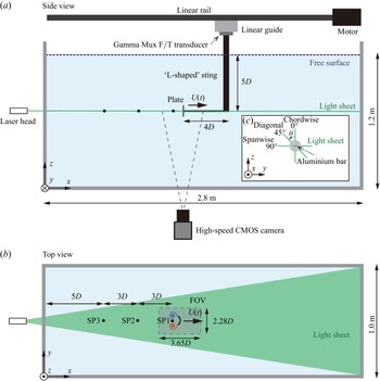


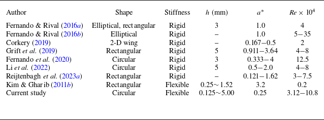
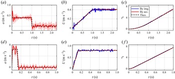


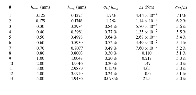


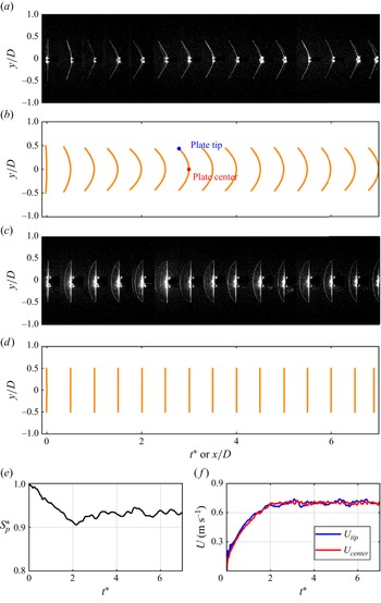


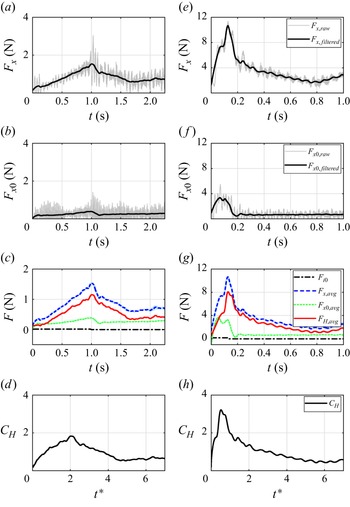


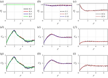


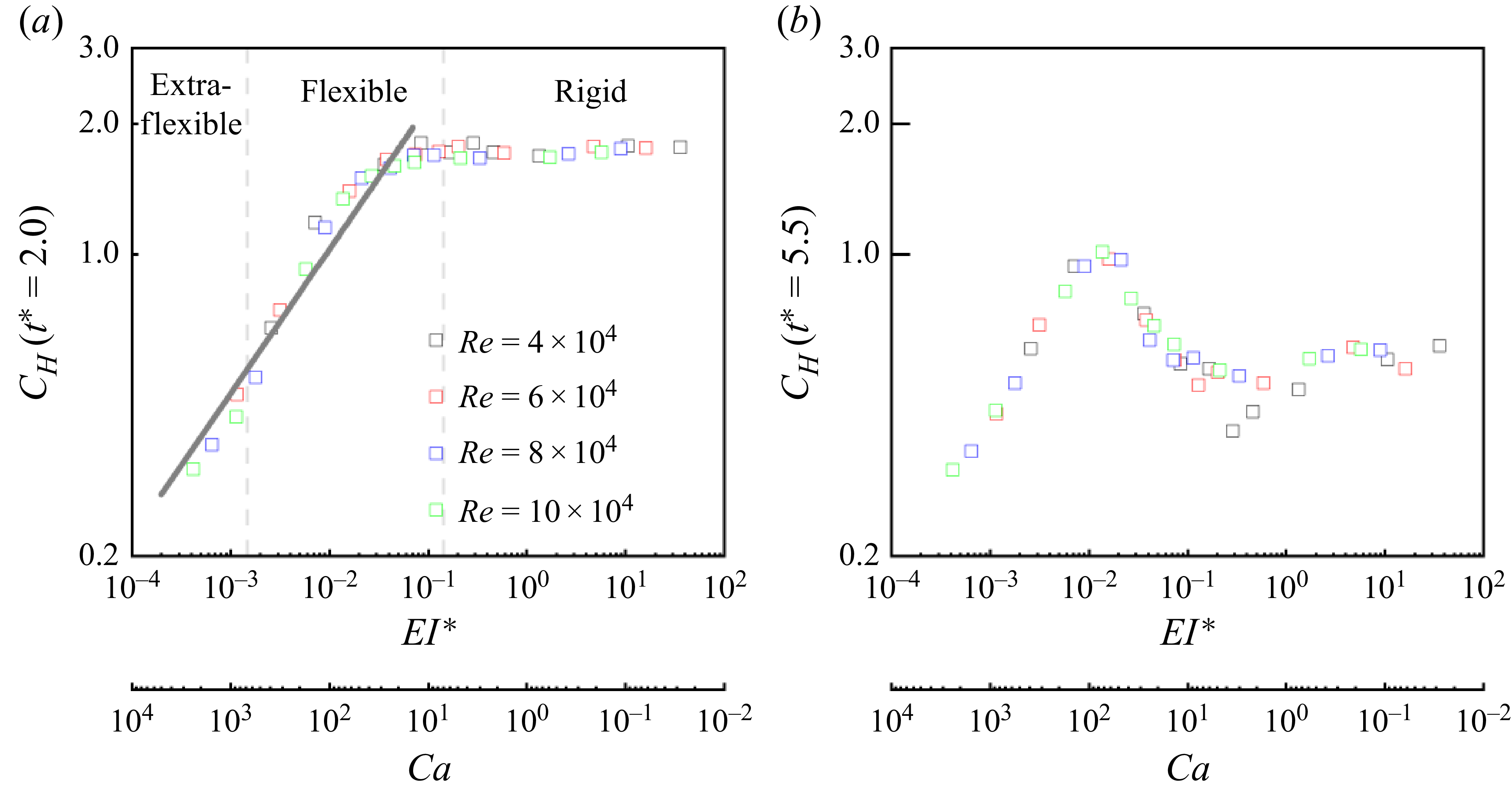


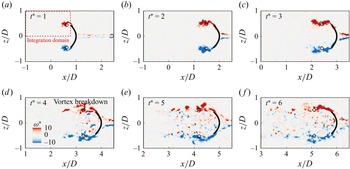


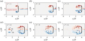


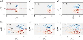


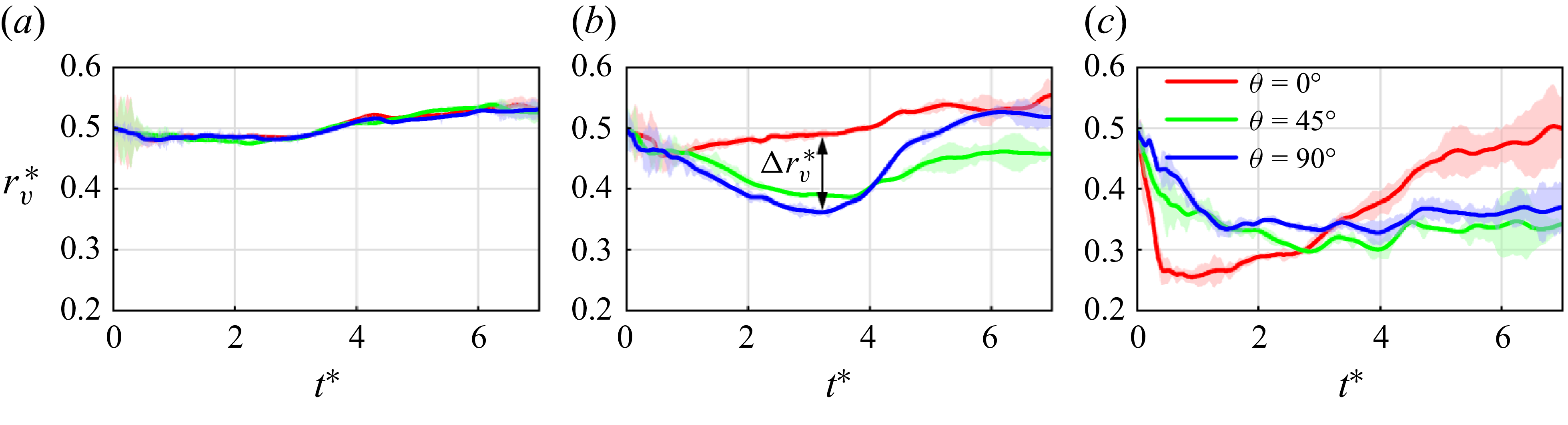


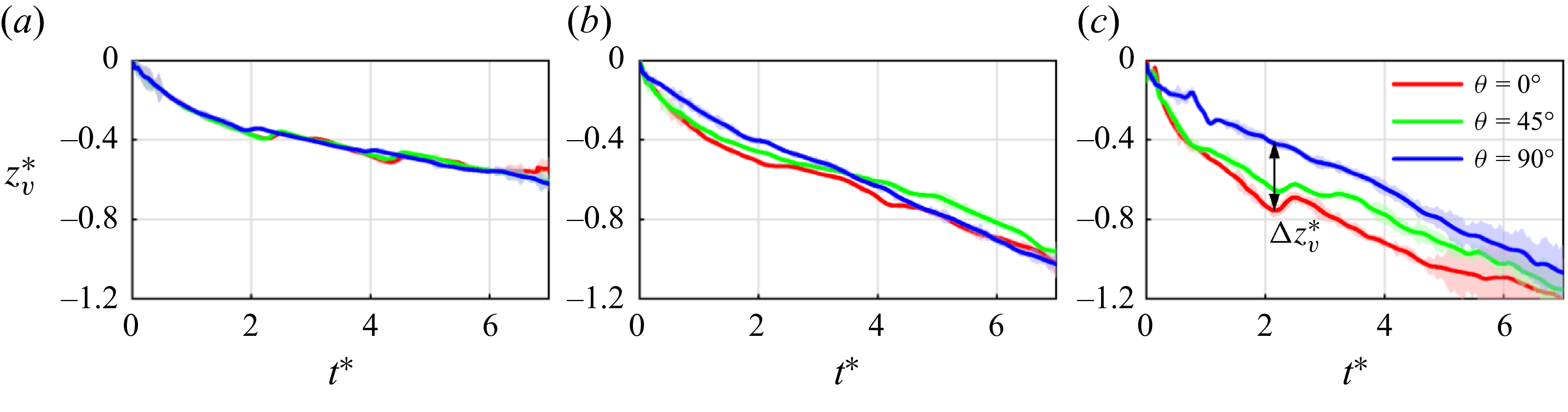


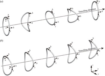
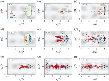


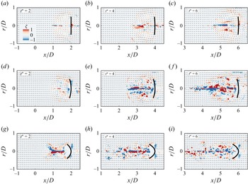


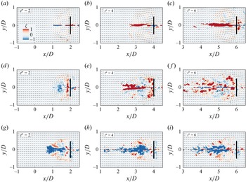


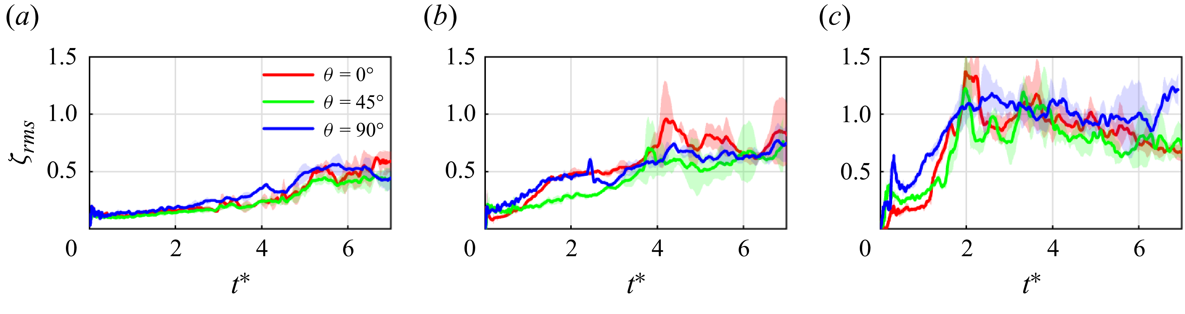


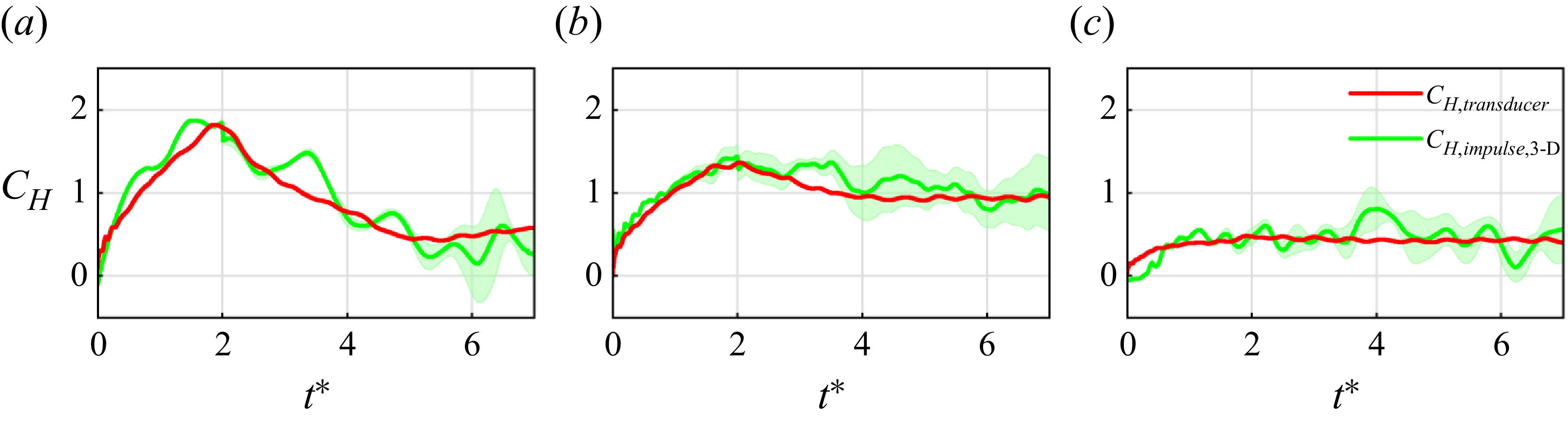


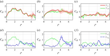


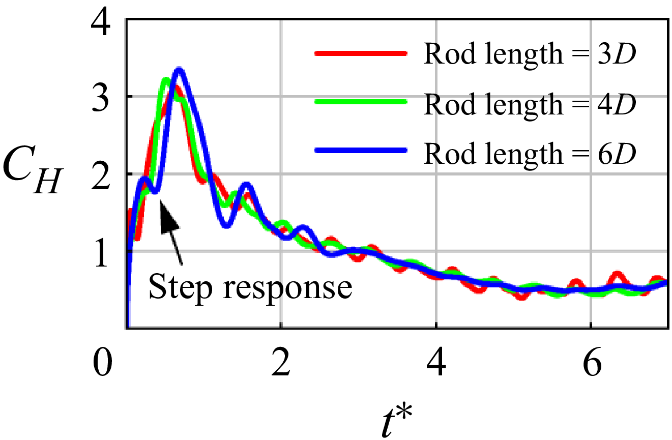


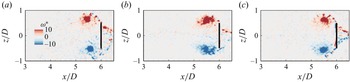


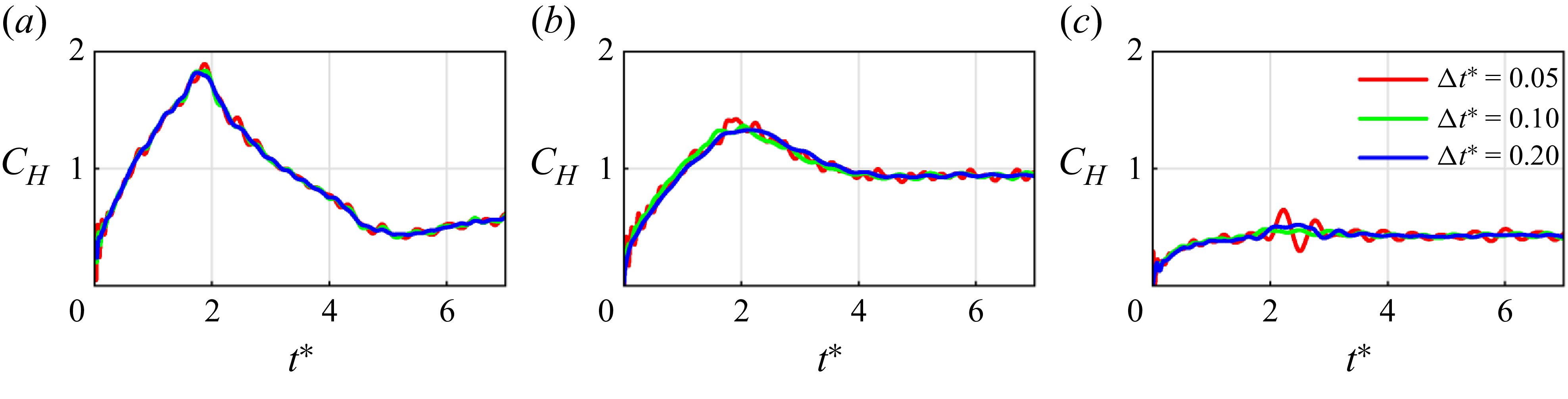


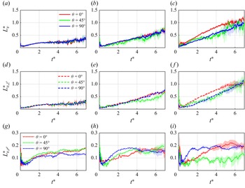


 Open access