


1. Introduction
Radiation pressure acceleration (RPA) of ions has attracted significant attention in the last two decades (Esirkepov et al. Reference Esirkepov, Borghesi, Bulanov, Mourou and Tajima2004; Pegoraro & Bulanov Reference Pegoraro and Bulanov2007; Robinson et al. Reference Robinson, Zepf, Kar, Evans and Bellei2008; Chen et al. Reference Chen, Pukhov, Yu and Sheng2009; Macchi, Veghini & Pegoraro Reference Macchi, Veghini and Pegoraro2009; Chen et al. Reference Chen, Kumar, Pukhov and Yu2011; Palmer et al. Reference Palmer, Dover, Pogorelsky, Babzien, Dudnikova, Ispiriyan, Polyanskiy, Schreiber, Shkolnikov and Yakimenko2011; Dollar et al. Reference Dollar, Zulick, Thomas, Chvykov, Davis, Kalinchenko, Matsuoka, McGuffey, Petrov and Willingale2012; Khudik et al. Reference Khudik, Yi, Siemon and Shvets2014; Eliasson Reference Eliasson2015; Wan et al. Reference Wan, Pai, Zhang, Li, Wu, Hua, Lu, Joshi, Mori and Malka2018; Wang, Khudik & Shvets Reference Wang, Khudik and Shvets2021). The two important characteristics of RPA are the higher laser energy conversion to the ions and the quality of the ion energy spectrum. Due to these reasons the ion beams accelerated by the radiation pressure can have ultrashort pulse duration, and extremely high peak energy needed for applications in many areas (Roth et al. Reference Roth, Cowan, Key, Hatchett, Brown, Fountain, Johnson, Pennington, Snavely and Wilks2001; Borghesi et al. Reference Borghesi, Bulanov, Campbell, Clarke, Esirkepov, Galimberti, Gizzi, MacKinnon, Naumova and Pegoraro2002; Atzeni & Meyer-ter Vehn Reference Atzeni and Meyer-ter Vehn2004; Li et al. Reference Li, Séguin, Frenje, Rygg, Petrasso, Town, Amendt, Hatchett, Landen and Mackinnon2006; Mackinnon et al. Reference Mackinnon, Patel, Borghesi, Clarke, Freeman, Habara, Hatchett, Hey, Hicks and Kar2006; Daido, Nishiuchi & Pirozhkov Reference Daido, Nishiuchi and Pirozhkov2012; Honrubia & Murakami Reference Honrubia and Murakami2015) including ion beam therapy (Malka et al. Reference Malka, Fritzler, Lefebvre, d’Humières, Ferrand, Grillon, Albaret, Meyroneinc, Chambaret and Antonetti2004).
The idea of using plasma as a medium to accelerate charged particles under electromagnetic waves and the use of the photon beams for sailing are not new; they were already being discussed in the 1950s (Veksler Reference Veksler1957; Garwin Reference Garwin1958; Tsu Reference Tsu1959). The proposal to use lasers for interstellar travel was discussed by R. Forward in 1962 (McInnes Reference McInnes1999; Forward Reference Forward1984) and later on reinvented by Marx (Reference Marx1966), who first worked out the equation by considering a simple model of a mirror accelerated by a laser pulse (Marx Reference Marx1966; Forward Reference Forward1984). This line of thought is not in the realm of science fiction, and the photon sail can accelerate the interstellar probe to approximately 20 % of the velocity of light within minutes (Heller & Hippke Reference Heller and Hippke2017). The idea of RPA also has its genesis in the work of Einstein when he studied the reflection of light from a mirror and deduced that the ratio $E/\omega$ , where $E$
 is the electric field and $\omega$
 is the frequency of the light, is an invariant. This invariant was later found out to be the Planck constant ($E=\hbar \omega$
 ), which Einstein subsequently used to explain the photoelectric effect (Pauli Reference Pauli1981). With the availability of ultraintense lasers $I_l \sim 10^{23}\,\textrm {W}\,\textrm {cm}^{-2}$
 , in the near future (xce 2017; cil 2019; vul 2020; eli 2021), the RPA of ions has the potential to produce high-energy ion beams with higher energy conversion efficiency compared with other mechanisms of laser-driven ion acceleration (Forslund & Shonk Reference Forslund and Shonk1970; Silva et al. Reference Silva, Marti, Davies, Fonseca, Ren, Tsung and Mori2004; Haberberger et al. Reference Haberberger, Tochitsky, Fiuza, Gong, Fonseca, Silva, Mori and Joshi2012; Liu et al. Reference Liu, Weng, Li, Yuan, Chen, Mulser, Sheng, Murakami, Yu and Zheng2016). Apart from the technological requirements for the efficient RPA of ions, e.g. the need for the high-contrast, large focal spot size of the ultraintense laser pulse, the issue of the transverse instabilities remains important. The onset of the transverse instabilities limits the effectiveness of the RPA of ions. The onset and physical mechanisms of these transverse instabilities have been recently studied focusing on the intrinsic origin of the instability (Pegoraro & Bulanov Reference Pegoraro and Bulanov2007; Khudik et al. Reference Khudik, Yi, Siemon and Shvets2014; Eliasson Reference Eliasson2015; Wan et al. Reference Wan, Pai, Zhang, Li, Wu, Hua, Lu, Joshi, Mori and Malka2018, Reference Wan, Andriyash, Lu, Mori and Malka2020). Several methods, e.g. tailored electromagnetic pulses with sharp intensities (Pegoraro & Bulanov Reference Pegoraro and Bulanov2007), modulation of the RPA (Bulanov et al. Reference Bulanov, Esirkepov, Pegoraro and Borghesi2009) and the use of surface modulated targets (Chen et al. Reference Chen, Kumar, Pukhov and Yu2011) have been proposed to alleviate the influence of the transverse instabilities on the RPA of ions. Moreover, in the ultrarelativistic regime of the laser plasma interaction, envisaged in eli (2021), cil (2019), xce (2017) and vul (2020), the effect of the radiation reaction (RR) force in the laser-driven electron dynamics has to be taken into account (Chen et al. Reference Chen, Pukhov, Yu and Sheng2010; Macchi et al. Reference Macchi, Tamburini, Pegoraro and Liseykina2011).
In this paper, we study not only the RPA of ions from the density modulated and structured targets, but we also study the influence of the RR force on the development of the transverse instabilities from density modulated and structured targets. This paper is organised as follows: In § 2.1, we discuss the parameters of the particle-in-cell (PIC) simulations, followed by the energy spectra of the accelerated ions in § 2.2. Afterwards, we analyse the Rayleigh–Taylor-like transverse instability (RTI) growth rate for surface modulated targets in § 3.1 and follow-up with the Fourier analysis of the ion density fluctuations in § 3.2. Before we conclude in § 4, we briefly show the results from a simulation run having a laser pulse with spatial Gaussian profile interacting with a target consisting of both density and surface modulations.
2. PIC simulations set-up and results
We first begin by showing the results on the RPA of protons in ultrarelativistic regimes from the density modulated and structured targets. Afterwards, we extend the results to the radiation dominated regime including the effect of the RR force on the RPA of protons from the density modulated and structured targets.
2.1. PIC simulations set-ups and shapes of structured and density modulated targets
For PIC simulations, we use the open source PIC code SMILEI (Derouillat et al. Reference Derouillat, Beck, Pérez, Vinci, Chiaramello, Grassi, Flé, Bouchard, Plotnikov and Aunai2018). We carry out two-dimensional (2-D) in space and three-dimensional (3-D) in velocity simulations employing a simulation box of size $L_x \times L_y = 18\lambda _L \times 10\lambda _L$ , where $\lambda _L = 0.8 \times 10^{-6}\,\textrm {m}$
 is the laser wavelength. Thus, for $\Delta x=\Delta y=0.06\lambda _L$
 , it yields $1800 \times 1000$
 cells in the simulation box. This resolution is comparable or smaller than the previous studies on ion acceleration (Esirkepov et al. Reference Esirkepov, Borghesi, Bulanov, Mourou and Tajima2004; Pegoraro & Bulanov Reference Pegoraro and Bulanov2007; Haberberger et al. Reference Haberberger, Tochitsky, Fiuza, Gong, Fonseca, Silva, Mori and Joshi2012; Zigler et al. Reference Zigler, Eisenman, Botton, Nahum, Schleifer, Baspaly, Pomerantz, Abicht, Branzel and Priebe2013; Wang et al. Reference Wang, Khudik and Shvets2021). The time step of the simulation is $4.19\, \times 10^{-2} \tau _L$
 , where $\tau _L = 2{\rm \pi} /\omega _0 = 2.67$
 fs is the laser period, corresponding to a total of $1.5\times 10^{4}$
 iterations. For the sake of computational efficiency, we take protons instead of high-Z ions. We use 16 particles per cells per species for PIC simulations. The plasma is fully ionised with a maximum density of $n_e = 250\,n_c$
 , where $n_c = \omega _0^2 m_e/4{\rm \pi} e^2= 4.36\times 10^{23}\,\textrm {cm}^{-3}$
 is the non-relativistic critical density for the laser pulse of frequency $\omega _0 = 2.36 \times 10^{15}\,\textrm {s}^{-1}$
 corresponding to the Ti:Sa laser pulse system. Here $e$
 and $m_e$
 are the electronic charge and mass, respectively. Plasma ions are assumed to be cold, however, the plasma electrons have a small temperature, $T_e \sim 10^{-3}\,m_e c^2$
 , where $c$
 the velocity of light in vacuum. We employ a moving window in our PIC simulations. At the onset of the moving window, the circularly polarised laser pulse injection into the simulation is turned off. Consequently, we have a finite laser pulse duration in our simulations. The laser pulse is turned off when the moving window starts in the simulations, effectively limiting the pulse duration. For the flat target, we have pulse duration $t/\tau _L \approx 35$
 fs and for density and surface modulated targets, we have $t/\tau _L \approx 30$
 fs. Since the velocity of the moving window, $\upsilon _\textrm {mov}$
 , closely follows the group velocity of the laser pulse which in turn depends on the laser and plasma parameters, we have different velocities in the range $\upsilon _\textrm {mov}=(0.67-0.84) c$
 of the moving window. The optimum target thickness for the RPA is given by $\xi \simeq a_0$
 , where $\xi = {\rm \pi}n_e d /n_c \lambda _L$
 , $d$
, $d$ is the target thickness and $a_0=e E_0/m_e \omega _0 c$
 is the dimensionless amplitude of the circularly polarised laser pulse (Macchi et al. Reference Macchi, Veghini and Pegoraro2009). For $a_0=150$
 and $n_e = 250\,n_c$
 , we get $d \simeq 0.19\lambda _L$
 . Notwithstanding technological improvements, manufacturing of the structured targets is always challenging. Thus, from the point of view of manufacturing structured targets and limiting the deleterious prepulse effects, thicker targets $(d \ge 1.0 \lambda _L)$
 may be preferred over ultrathin targets ($d \ll 1.0\lambda _L$
 ) for performing experiments.
Since we are interested in studying the physics of competitive mode feeding of the RTI-like transverse instabilities, we exclude other effects occurring due to the spatiotemporal shapes of the laser pulse. Figure 1 shows the targets with different modulations. The profiles in figure 1 are described mathematically as follows: In figure 1(a) the density modulated target with width ($d=1.0\lambda _L$ ) has a spatial density profile, $n(x,y) = n_e a_m [3+\cos (k_m y)]/2$
 , where $n_e=250\,n_c$
 . This yields minimum density $n_{\min } = a_m\,n_{e}$
 . Figure 1(b) describes the rippled plasma density target with the width ($d=1.0\lambda _L$
 ), with the ripples being located in the region, $d + a_m \cos (k_m y) \leq x \leq d + a_m$
 , having the spatial density as $n(x,y) = n_e [a_m\cos (k_my)-a_m]$
 . Figure 1(c) depicts the structured target with rectangular grooves, which are located in the region $d - a_m \leq x \leq d + a_m$
 , and the spatial density profile reads as, $n(x,y) = n_e [a_m\cos (k_my)-a_m]$
 . Finally, figure 1(d) depicts the target with ripples imposed on the left-hand side. The target has ripples localised in the region, $d - a_m \cos (k_m y) \leq x \leq d + a_m$
 , with a constant plasma density $n_e$
 in this case. The targets with a width $d=1.0\lambda _L$
 are located in the region $1.0\lambda _L \leq x \leq 2.0\lambda _L$
 , while the targets with a width $d=2.0\lambda _L$
 are located in $1.0\lambda _L \leq x \leq 3.0\lambda _L$
 in all cases. Parameter $a_m$
 is a dimensionless number showing the modulations in the density, while $k_m$
 is normalised with the laser wavevector $k_L$
 in all cases. We not only change the wavelength of the modulations, $\lambda _m$
 (normalised to $\lambda _L$
 ), but also the amplitude of the modulations $a_m$
 in figure 1(a–d).
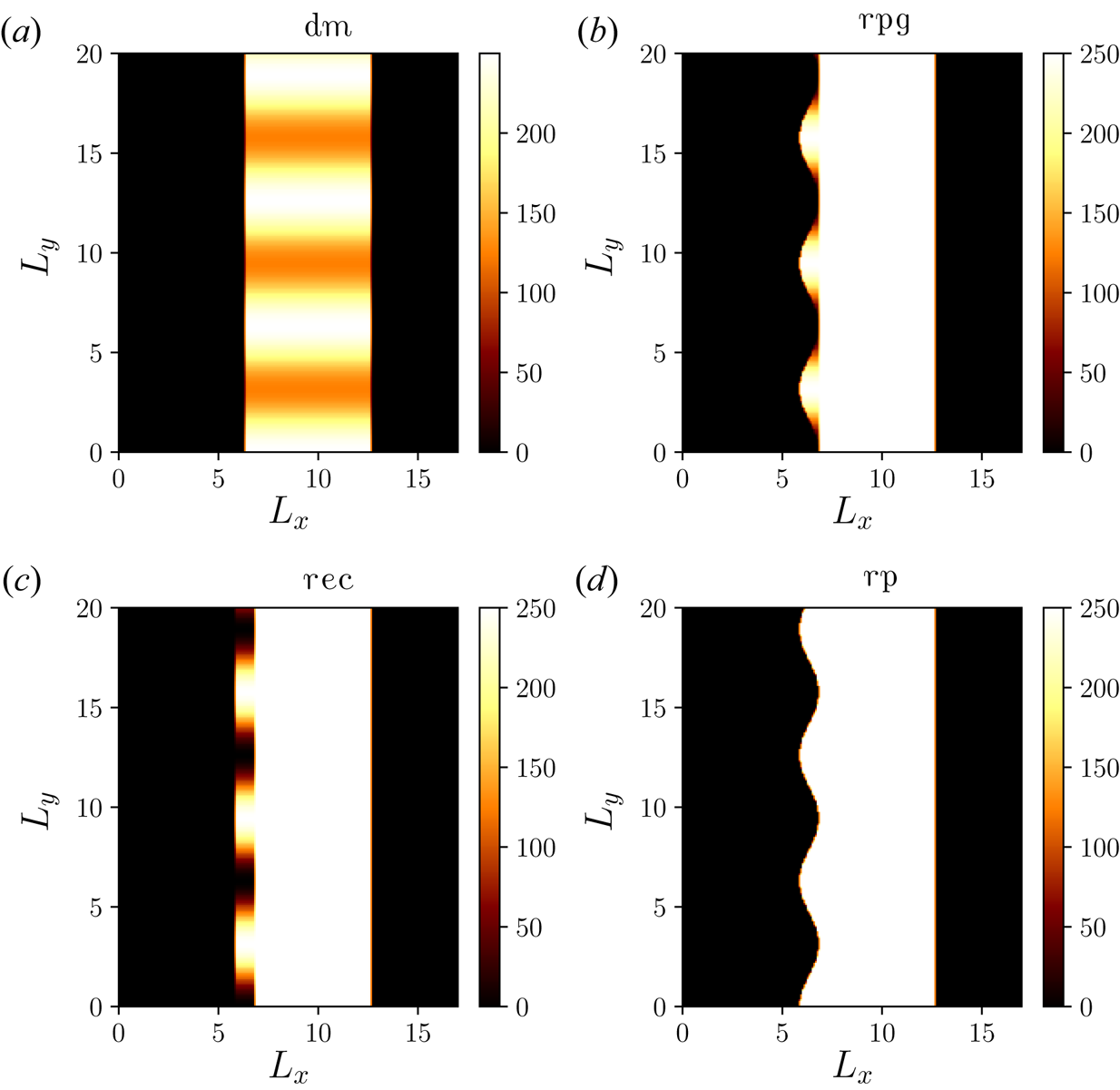
Figure 1. (a) Density modulated target (dm), (b) rippled target with changing plasma density (rpg), (c) surface modulated target with rectangular grooves (rec) and (d) rippled target with constant plasma density (rp). The colourbar denotes the normalised plasma density $n_e/n_c$ .
.
2.2. Energy spectra of ions
Figure 2 shows the energy spectra of different targets. One can immediately see that modulating the target density leads to improvement not only in the quality of the energy spectra captured in the full width at half maximum (FWHM), but in the case of the density modulated target (figure 1a), it also results in higher energy gain with significantly smaller FWHM ($\Delta E/E\sim 12\,\%$ ) in comparison with other modulated targets and remarkably smaller compared with the flat target ($\Delta E/E\sim 26\,\%$
 ) case. The lower number of accelerated ions in the case of the density modulated target can be attributed to both lower target mass in the beginning and also a slight loss (${\sim }4\,\%$
 ) of the target mass in the interaction process (see supplementary material available at https://doi.org/10.1017/S0022377821001070). The maximum energy of protons in figure 2 are slightly smaller than the analytical scalings. The analytical scaling of proton energy, reproduced here again for completeness, reads as $E_k= A m_pc^2(\gamma _f -1), \gamma _f=(1-\beta _f^2)^{-1/2}, \beta _f=[(1+\mathcal {E})^2-1]/[(1+\mathcal {E})^2+1]$ $\textrm{and}\, \mathcal {E}=2 {\rm \pi}(Z/A)(m_e/m_p)\, a_0^2\, \tau / \xi$
 , where $m_p$
 is the proton mass, $\tau$
 is measured in the units of the laser period, $\tau _L$
 , and $Z$
 and $A$
 are the atomic and mass numbers, respectively (Macchi et al. Reference Macchi, Veghini and Pegoraro2009). For the flat target ($\tau =35$
 ) in figure 2, $E_k\sim 1.01$
 GeV while for the density modulated target ($n_e^{\text {max}}=125 n_c, \tau =30$
 ), it yields $E_k\sim 2.05$
 GeV. These values are a bit higher than observed in figure 2. As expected, the lower plasma density for the density modulated target leads to higher proton energy gain, but it alone cannot account for the lower FWHM of the proton energy spectrum observed in figure 2. Since, the modulations in the ion beam spectra are a good evidence of the growth of the RTI (Chen et al. Reference Chen, Pukhov, Yu and Sheng2010; Palmer et al. Reference Palmer, Schreiber, Nagel, Dover, Bellei, Beg, Bott, Clarke, Dangor and Hassan2012; Sgattoni et al. Reference Sgattoni, Sinigardi, Fedeli, Pegoraro and Macchi2015), it is apparent that the use of a density modulated and structured target is efficient in suppressing the long-wavelength modes of the RTI-like interchange instabilities (see movies). We explain this in terms of the competitive feeding of different modes in the RPA of protons later in § 3.2. Figure 3 shows a snapshot from the movies (see also supplementary movies) on the ion density and laser electric field evolutions. One can immediately notice the onset of the RTI-like instabilities for the flat-target case (figure 3b) while the density modulated target (figure 3a) does not show the surface rippling associated with the RTI-like instabilities leading to the breakup of the target at later times.
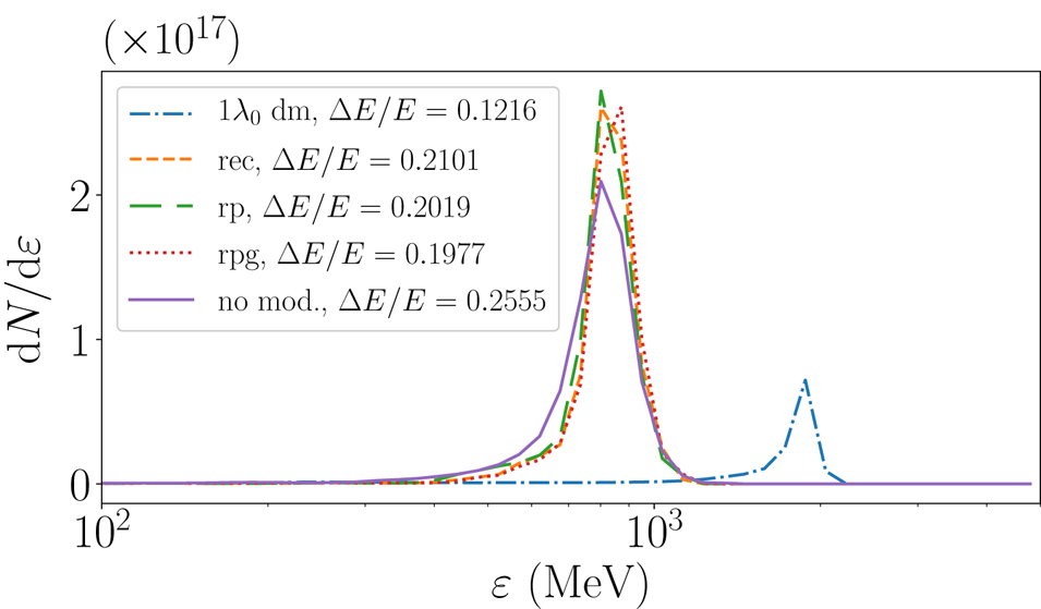
Figure 2. Kinetic energy of ions for different targets from figure 1 with modulation parameters, $k_m=2$ and $a_m=0.25$
 at $t/\tau _L = 440$
 . The other parameters are $a_0=150, n_e=250 n_c$
 and $d=1.0\lambda _L$
 in each case. The $y$
 axis represents the proton numbers, $N$
 per unit length. Moving window velocities are $\upsilon _\textrm {mov} = 0.8\, c$
 for dm target, and $\upsilon _\textrm {mov}=0.75\,c$
 for surface modulated and flat targets.
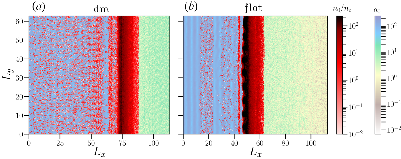
Figure 3. Evolution of the ion density and the normalised laser electric field $a_0$ for (a) a density modulated target ($k_m=2$
 , $a_m=0.25$
 ) and (b) the flat target, for $a_0=150$
 . Both targets have $d=1.0\lambda _L$
 width. The results are shown at $t/\tau _L = 144$
 . The other parameters are the same as in figure 2.
The stronger impact on the proton energy spectrum in the case of the density modulated target (figure 1a) points to the physical mechanism of the RTI-like interchange instability in the RPA regime of involving the coupling of both electron and ion modes (Wan et al. Reference Wan, Pai, Zhang, Li, Wu, Hua, Lu, Joshi, Mori and Malka2018). Not only the choice of the modulation wavevector $k_m=2$ , but also the choice of modulation amplitude $a_m$
 affect the late-time evolution of the ion energy spectrum. Figure 4 captures this dependence showing the evolution of the FWHM dm target for different modulation parameters. We record $E_{\textrm {max}}$
 and its FWHM at every simulation time step. Figure 4 shows these discrete data points (raw-data method) together with the Gaussian fitting (Gaussian fit method) of the simulation results. The difference between the two methods (Gaussian fit and raw data methods) can be attributed to the lack of clear single peak formation in the energy spectra, especially at early- and late-times. We also take into account error propagation of the Gaussian fitting. On defining the energy spread as $V=\Delta E/E$
 , the error in energy spread $\sigma _V$
 can be estimated as $\sigma _V=\sqrt {(\sigma _{\Delta E}/E)^2 + (\sigma _E \Delta E /E^2)^2}$
 , where $\sigma _E$
 and $\sigma _{\Delta E}$
 represent the standard deviations in the energy and the energy spread, respectively, of the ion beam. The oscillations in the energy spectra occur because the FWHM and $E_{\textrm {max}}$
 in figure 4 do not show the same temporal development. The stretching of the oscillations in the ion energy spectra is related to the speed of the target relative to the E-field of the laser, and the amplitude of the energy oscillations is related to the wavevector of the density modulations. For comparison we also plot the FWHM of a flat target in figure 4. One can notice that in the case of the flat target, the FWHM increases with time, while for the density modulated target (figure 4b), it remains lower for a longer duration. On changing the amplitude of the density modulation ($a_m=0.25$
 ) as in figure 4(d), the FWHM remains lower and stable for longer durations but shows the disruption in the ion energy spectrum at later times. Thus, an optimisation in value of modulation parameters is required.
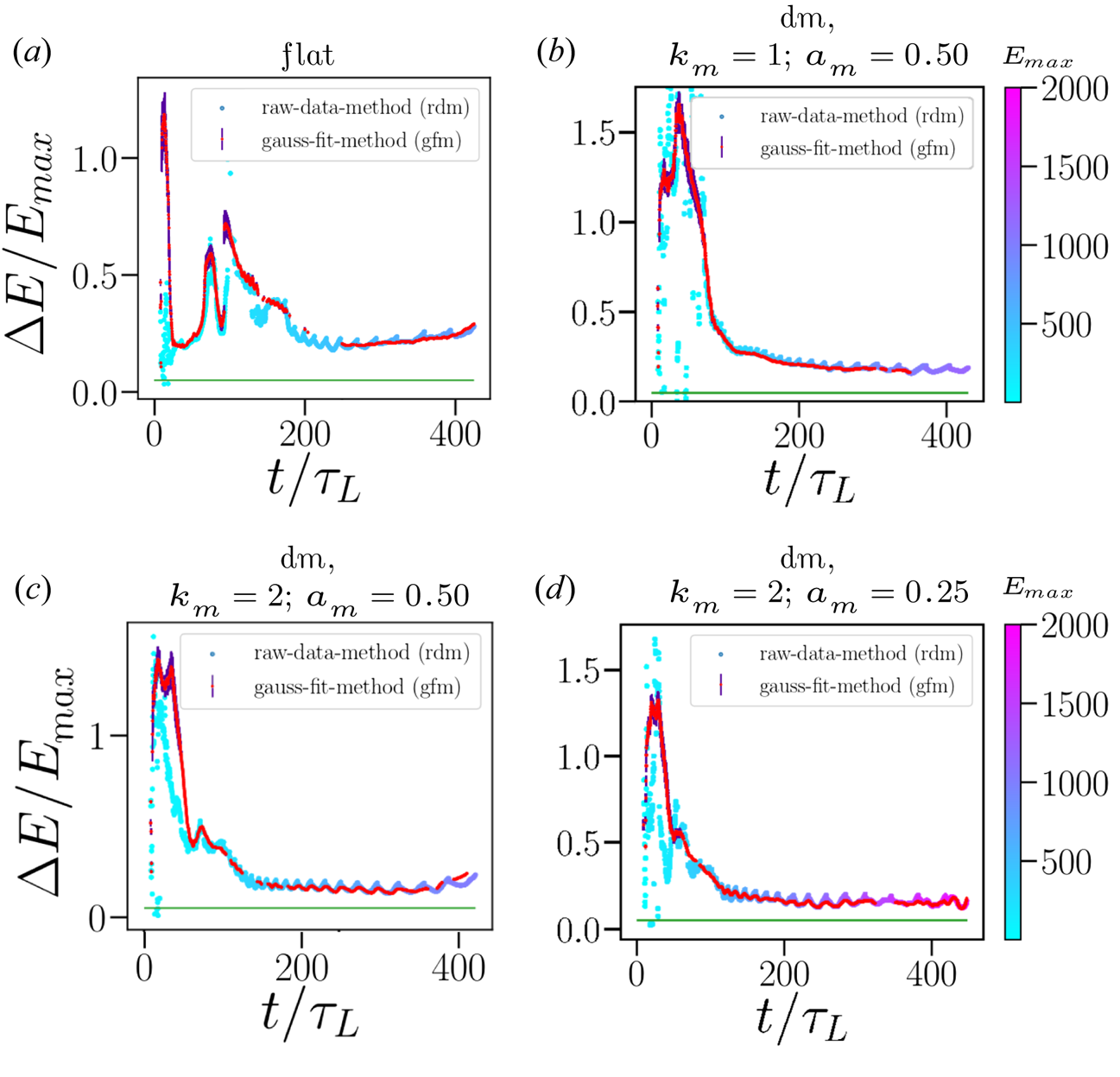
Figure 4. Evolution of the $\Delta E/E_{\textrm {max}}$ with time. The colourbar denotes the $E_{\textrm {max}}$
 (in MeV) in each case. (a) The flat target, (b) dm with $k_m=1$
 , $a_m=0.50$
 , (c) $k_m=2$
 , $a_m=0.50$
 and (d) $k_m=2$
 , $a_m=0.25$
 . The target width is $d=1.0\lambda _L$
 in each case. The green line is the sought limit of $\Delta E/E_{\textrm {max}} = 0.05\, (5\,\%)$
 . The other parameters are the same as in figure 2.
2.3. Parameter maps for the optimised RPA of ions
Figure 5 shows the maps depicting the dependence of the proton energy and its spread on $a_m$ and $k_m$
 for the density modulated targets with different thicknesses. Figure 5(a,b) show the FWHM and maximum ion energies for a density modulated target with the target thicknesses, $d=1.0\lambda _L$
 and $d=2.0\lambda _L$
 , respectively. These maps are generated from the 12 simulation data points interpolated using a cubic interpolation scheme. One can observe a few trends quickly. First, for the thinner target ($d=1.0\lambda _L$
 , figure 5a,b), the optimum range for $a_m$
 extends to $a_m \approx 0.35$
 while the range of $k_m$
 shrinks to $k_m \approx 3$
 . For a thicker target ($d=2.0\lambda _L$
 , figure 5c,d), the preimposed modulations have only a beneficial effect for $a_m \lesssim 0.25$
 and $k_m \in (2,5)$
 . This can be understood based as follows: for a fixed $a_0$
 , the thinner target has lower target mass and consequently lower $\xi$
 , resulting in the dominance of the RPA mechanism and higher ion acceleration energies for the $d=1.0\lambda _L$
 target (compare figures 5b and 5d). Large $a_m$
 and $k_m$
 facilitate stronger absorption of the laser pulse, resulting in the stronger electron heating that can lower the RPA of ions and degrade the FWHM of the ions for a thick target ($d=2.0\lambda _L$
 ), presumably due to the TNSA process playing a role. Further increasing the $a_m$
 for a $d=1.0\lambda _L$
 target, one again reaches the regime of stronger laser penetration and heating of the plasma electrons resulting in lower proton energy gain and degradation in the proton spectrum quality possibly due to the effect of the TNSA process (Andreev et al. Reference Andreev, Kumar, Platonov and Pukhov2011; Zigler et al. Reference Zigler, Eisenman, Botton, Nahum, Schleifer, Baspaly, Pomerantz, Abicht, Branzel and Priebe2013; Ferri et al. Reference Ferri, Thiele, Siminos, Gremillet, Smetanina, Dmitriev, Cantono, Wahlström and Fülöp2020).
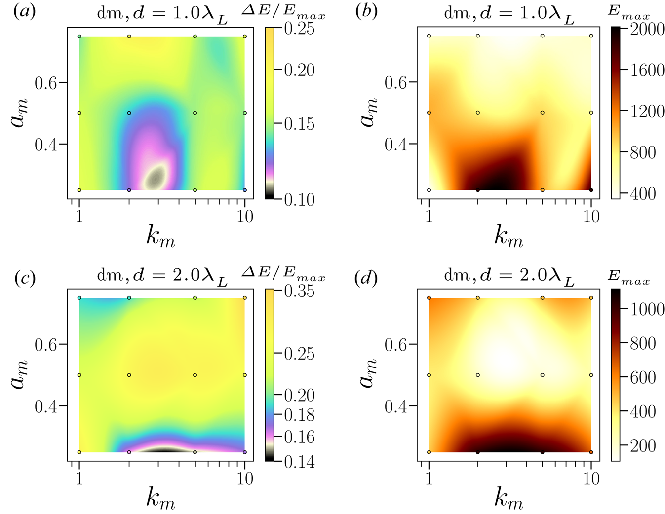
Figure 5. Parameter maps for the ion energy spectra ($\Delta E/E_{\textrm {max}}$ , panels (a,c)) and ion acceleration energies $E_{\textrm {max}}$
 (in MeV, panels (b,d)) with $a_m$
 and $k_m$
 for the density modulated target. Panels (a,b) and (c,d) correspond to the targets with $d=1.0\lambda _L$
 and $d=2.0\lambda _L$
 widths, respectively. Please notice that here and afterwards, unless stated otherwise, $k_m$
 is normalised with the laser wavevector $k_L$
 , while $a_m$
 is a dimensionless number as mention before in § 2.1. The small circles are data points used for the interpolation. The other parameters are same as in figure 2.
Figure 6 shows the same parameter maps for other surface modulation shapes as in figure 1. Here, the parameter maps are generated from 16 simulation data points. First, it can be seen that all maximum energy peaks are roughly identical, i.e. all surface modulated targets have similar values of $E_{{\textrm {max}}}$ , which is smaller compared with the density modulated target as shown in figure 5. The trends for the optimum value of $k_m$
 are similar in the cases of rectangular and rippled grooves, but a nonlinear behaviour for the rippled grooving with varying (rpg) density is observed. In general, a larger value of $a_m$
 , e.g. $a_m \ge 0.2$
 , leads to a smaller FWHM of the ion energy spectra with $k_m$
 being largely centred between $2 < k_m < 5$
 (except for the rpg shape). The corresponding values of $E_{{\textrm {max}}}$
 are essentially following the same pattern as for the corresponding FWHM of the energy spectra. The higher acceleration energies for larger $a_m$
 and $k_m \le 2$
 , can be explained by the locally enhanced electric field and higher absorption of the laser field in different targets. The different behaviour in the three cases exemplify the different evolutions of the RTI-like interchange instabilities due to perturbations fed by different structured targets. To study this we carry out fast Fourier transforms (FFT) of the ion plasma densities and the results are discussed in § 3.2.

Figure 6. Parameter maps for $a_m$ and $k_m$
 for target thickness $d=1.0\lambda _L$
 . The colourbars denote (a,c,e) $\Delta E/E_{\textrm {max}}$
 and (b,d,f) $E_{\textrm {max}}$
 . Panels (a,b), (c,d) and (e,f) show structured targets viz. (a,b) rec, (c,d) rp, (e,f) rpg, respectively. The other parameters are same as in figure 2.
2.4. RR effects on the RPA of ions from density modulated and structured targets
We also performed simulations including the effect of the RR on the RPA of ions from density modulated and structured targets. The SMILEI code includes both Landau–Lifshitz and quantum description of the RR force (Derouillat et al. Reference Derouillat, Beck, Pérez, Vinci, Chiaramello, Grassi, Flé, Bouchard, Plotnikov and Aunai2018). For this we used the same structured and density modulated targets as in § 2.1. Figure 7 shows the results on the ion energy spectra from the structured and density modulated targets for $a_0=250$ . One can see that the use of the density modulated and structured targets results in the lower FWHM of ions compared with a flat target. However, compared with the other structured targets, the biggest reduction occurs in the case of the density modulated target which shows the FWHM of the ion energy spectrum to be ${\sim }15\,\%$
 . For this value of $a_0$
 , one may begin to see the influence of the RR force in laser–plasma interaction. In order to further examine the role of the RR force and the target widths on ion acceleration from the density modulated target, we show in figure 8 and figure 9 the best results with RR ($a_0=250$
 for figure 8 and $a_0=350$
 for figure 9) for the two target widths (panels (a) and (b)). In order to compare the results, we kept $a_m$
 and $k_m$
 same in figures 8(a) and 8(b) ($a_m=0.25$
 and $k_m=2$
 ) and also in figures 9(a) and 9(b) ($a_m=0.5$
 and $k_m=2$
 ). Moreover, we also show the results for $a_0=150$
 for comparison in each respective case, which facilitate the comparison with the respective no radiation reaction force limiting case since RR effects are significantly weaker at $a_0=150$
 . For a target with $d=1.0\lambda _L$
 width (figures 8a and 9b) in each case, the ion energy gain is higher compared with the thicker target $d=2.0\lambda _L$
 (figures 8c and 9d). Also ions gain larger energies for dm (dashed green line) target compared with the flat target (solid red line) in figures 8 and 9. These trends can be explained on the basis of the lower target mass in respective cases, since the lower target mass is expected to result in ions acquiring higher energies in accordance with the scalings of RPA of ions; this is also discussed in § 2.2 (Macchi et al. Reference Macchi, Veghini and Pegoraro2009). Also with the inclusion of the RR force, the density modulated target continues to show the higher ion energy gain and lower FWHM, compared with the flat target case. However, the trend with respect to FWHM of the ion energy spectra shows interesting features. The ion energy spread is lower for the thicker target; the FWHM ${\sim }12\,\%$
 for $d=2.0\lambda _L$
 width at $a_0=250$
 in figure 8(b). But it is smaller for the thinner target ($d=1.0\lambda _L$
 ) case when the RR force is strong, see figure 9. Thus, the thinner target (figure 9a) shows not only higher ion energy (${\sim }2.5$
 GeV) but also lower energy spread (FWHM $=14\,\%$
 ), yielding the best results in the radiation dominated regime. Moreover, the density of the accelerated ion bunch is also higher at higher $a_0$
 in figure 9 compared with figure 8. This highlights the nonlinear role of RR force for the density modulated target.

Figure 7. Kinetic energy of ions for different targets with modulation parameters $k_m=2$ , $a_m=0.25$
 , at $t/\tau _L = 314$
 with RR ($a_0=250$
 ). The target width is $d=1.0\lambda _L$
 in each case. Moving window velocities are $\upsilon _\textrm {mov} = 0.84\, c$
 for dm target, and $\upsilon _\textrm {mov}=0.8\,c$
 for surface modulated and flat targets.

Figure 8. Kinetic energy of ions for different modulations for $k_m=2$ , $a_m=0.25$
 , at (a) $t/\tau _L = 314$
 ($d=1.0\lambda _L$
 target width) and (b) $t/\tau _L = 394$
 ($d=2.0\lambda _L$
 target width) with RR ($a_0=250$
 ). The dm (blue dotted) and no modulation (orange dashed) lines are for $a_0=150$
 . Panel (a), moving window velocities are $\upsilon _\textrm {mov}= 0.80\,c\, (0.75\,c)$
 for flat, and $\upsilon _\textrm {mov} = 0.84\,c\, (0.80\,c)$
 for dm targets at $a_0=250$
 ($a_0=150$
 ). Panel (b), moving window velocities are $\upsilon _\textrm {mov} = 0.75\,c\, (0.75\,c)$
 for flat, and $\upsilon _\textrm {mov} = 0.75\,c \,(0.67\,c)$
 for dm targets at $a_0=250$
 ($a_0=150$
 ).
).

Figure 9. Kinetic energy of ions for different modulations, $k_m=2$ , $a_m=0.50$
 , at (a) $t/\tau _L = 307$
 for $d=1.0\lambda _L$
 target width, (b) $t/\tau _L = 394$
 for $d=2.0\lambda _L$
 target width with RR ($a_0=350$
 ). The dm (blue dotted) and no modulation (orange dashed) lines are for $a_0=150$
 . For $a_0=350$
 , we have $\upsilon _\textrm {mov} = 0.80\,c$
 for flat targets (in both panels); for dm targets, $\upsilon _\textrm {mov} = 0.84\,c$
 and $\upsilon _\textrm {mov} = 0.75\,c$
 in (a,b), respectively. Moving window velocity is same for $a_0=150$
 as in figure 8.
3. Interpretation of the PIC simulation results
First we briefly discuss the theoretical analysis of the RTI-like transverse instability from the surface modulated targets. Afterwards, we carry out the Fourier analysis of the ion density oscillation and discuss the development of the RTI-like transverse instability for density modulated and structured targets including the effect of the RR force.
3.1. Theoretical analysis of the transverse instability from surface modulated targets
To understand the behaviour of the transverse instability development, we calculate the growth rate of the RTI-like transverse instability in the RPA regime of ions for surface modulated targets. We wish to stress that although we follow the analysis of Pegoraro & Bulanov (Reference Pegoraro and Bulanov2007), we analytically also consider the effect of the preimposed density modulation on the development of the RTI-like instabilities, which was not considered before in Pegoraro & Bulanov (Reference Pegoraro and Bulanov2007) and Bulanov et al. (Reference Bulanov, Esirkepov, Pegoraro and Borghesi2009). Bulanov et al. (Reference Bulanov, Esirkepov, Pegoraro and Borghesi2009) considered the effect of modulating the laser field in PIC simulations and theoretically allowing for temporal variation of the target mass density in the transverse direction. This is different from our set-up since we impose modulations which have only spatial dependence. The evolution of these modulations, in feeding different modes of the RTI, is self-consistently simulated in PIC simulations. Most importantly, our emphasis on explaining the competitive feeding of different modes of the RTI was not done in earlier works. Notwithstanding the fact that the analysis is carried out for the surface modulated targets, one can also gain valuable physical insights for the density modulated target. We also do not take into account the variation in the radiation pressure (included in PIC simulations) due to the surface density modulations as studied before in lower $a_0$ and $n_0$
 limits (Eliasson Reference Eliasson2015; Sgattoni et al. Reference Sgattoni, Sinigardi, Fedeli, Pegoraro and Macchi2015). These studies suggest that preimposed surface modulations can lower the growth rate of short-wavelength perturbations of the RTI-like instability, and importantly the growth rate of this instability becomes higher around the laser wavelength due to the plasmonic effects (Eliasson Reference Eliasson2015; Sgattoni et al. Reference Sgattoni, Sinigardi, Fedeli, Pegoraro and Macchi2015). In our simulations (shown later in Fourier transforms), we do not observe these trends. It appears that for our parameters (higher $a_0$
 and $n_e$
 ), plasmonic effects discussed before are not dominant and consequently we can ignore them in the theoretical analysis. We briefly recall here the key points involved in the development of the analytical model to describe the interchange instability development for surface modulated targets. The equation of motion for a thin-foil target driven by the radiation pressure is written as

where $\mathcal {N}=(E^{2}/2{\rm \pi} )(1-{\beta })/(1+{\beta }),\,{\beta }={\upsilon }/c$ is the relativistically invariant pressure, $E$
 is the electric field of the laser pulse, $\epsilon _{i j k}$
 is the Levi-Civita tensor, $\sigma _{0} = n_{0} l_{0}$
 ($n_{0}$
 and $l_{0}$
 are the foil density and thickness, respectively) is the initial surface mass density, $p_{x,y}=m_{i}\, c\, \beta _{x,y}\gamma, \gamma = (1-\beta ^{2})^{-1/2}$
 , $\varphi,\, \zeta,\,\eta$
 is a set of curvilinear coordinate system to describe the evolution of a differential element of the thin foil. So motion of any point $\boldsymbol {r}$
 on the surface of the thin foil is defined as $\boldsymbol {r}[x(\xi,\,\zeta,\,\eta ),\,y(\xi,\,\zeta,\,\eta ),\,z(\xi,\,\zeta,\,\eta )]$
 . The $x$
 and $y$
 components of (3.1) read as (Pegoraro & Bulanov Reference Pegoraro and Bulanov2007; Bulanov et al. Reference Bulanov, Esirkepov, Pegoraro and Borghesi2009)


We investigate the stability of the thin foil in the long-wavelength limit (wavelength of perturbation higher than the thickness of the foil) by extending the approach of Pegoraro & Bulanov (Reference Pegoraro and Bulanov2007) for surface modulated targets. The stability of the thin-foil target against the long-wavelength perturbation is important as long-wavelength perturbations are detrimental and lead to the breaking of the target. We define $\varphi =\omega _{0}(t-x_{0}(t)/c)$ as a new variable. The initial conditions are

where $a_{m}$ denotes the depth of the modulation,Footnote 1 while $k_{m}$
 is the modulation wavevector. We again wish to stress that Pegoraro & Bulanov (Reference Pegoraro and Bulanov2007), Bulanov et al. (Reference Bulanov, Esirkepov, Pegoraro and Borghesi2009) take $y_{0}=\zeta$
 , thus not including the effect of preimposed density modulations on the growth of the RTI-like instabilities. The $x$
 component of the momentum on solving gives

For a constant amplitude pulse $E(\varphi )=E_{0},\, \Delta (\varphi )=\Delta _{0}$ , for $\omega _{0}\,t\ll (\lambda _{0}/\Delta _{0})$
 (early-time), we have $\varphi \approx \omega _{0} t$
 , and for $\omega _{0}\,t\gg (\lambda _{0}/\Delta _{0})$
 (late-time), we have $\varphi ^{3}=(\omega _{0}\,t) \, 6 \lambda _{0}^{2}/\Delta _{0}^{2}(1+ k_{m}^2l_{m}^2/4)$
 . On perturbing the equilibrium as

we get the following equations for the $x$ and $y$
 components (as in Pegoraro & Bulanov (Reference Pegoraro and Bulanov2007) and Bulanov et al. (Reference Bulanov, Esirkepov, Pegoraro and Borghesi2009)):


Assuming a perturbation of the form $\delta x,\,\delta y \sim \exp (\int _{0}^{\varphi }\varGamma (\varphi ^{'})\,\textrm {d}\varphi ^{'}-i q \zeta )$ , and $\partial \varGamma /\partial \varphi \ll \varGamma ^{2}$
 and $\varGamma \gg 1$
 , we get the growth rate of long-wavelength perturbations as $\varGamma = (\Delta (\varphi ) q/2{\rm \pi} )^{1/2}$
 . However, the actual growth of the perturbation for a constant amplitude pulse is written as $\delta x,\delta y \sim e^{\varGamma \varphi -i q \zeta }$
 . On using the relation between the variables $\varphi$
 and $t$
 for early- and late-times, we get the number of e-foldings for early and late-time growths of the perturbation (see also figure 10) as

One may note that the early-time asymptote of the instability shows no dependence on the preimposed modulations. This justifies the assumption of taking the equilibrium solution for a flat target and imposing the modulations in the initial conditions as done in (3.4a–e). From here the role of preimposed density modulations in reducing the growth rate of the RTI-like instabilities is apparent (see figure 10). In the case of no modulation $(k_{m}=0)$ , we recover the same growth of the perturbation as in Pegoraro & Bulanov (Reference Pegoraro and Bulanov2007) and Bulanov et al. (Reference Bulanov, Esirkepov, Pegoraro and Borghesi2009). One may observe that during the early stage, surface modulations do not play any role in the growth of the perturbation. However, for late-time of the instability development, modulations tend to lower the growth of the instability. In fact, for $|k_{m}l_{m}|\gg 4$
 (short-wavelength modulation), the growth of the long-wavelength modes of the instability reads as $N_{e}^{l} \propto t^{1/3}/ (k_{m}l_{m}/2)^{1/6}$
 . This clearly shows reduction in the growth of the short-wavelength perturbation, consistent with the results presented before (Eliasson Reference Eliasson2015; Sgattoni et al. Reference Sgattoni, Sinigardi, Fedeli, Pegoraro and Macchi2015). In the opposite limit $|k_{m}l_{m}|\ll 4$
 (long-wavelength modulation), there is no reduction in the growth rate of the long-wavelength perturbation. However, the introduction of the short-wavelength modulation amounts to selectively feeding the short-wavelength modes of the instability. This selective feeding can suppress the generation of the long-wavelength modes of the instability, which are detrimental for the stability of the target. In the opposite case of the preimposed long-wavelength density modulations, the long-wavelength modes of the instability grow faster to break the target. Consequently, one can expect to get lower energy spread in the ion energy spectra for the preimposed short-wavelength density modulations. Figure 6 qualitatively agrees with this scaling and shows better agreement for the rippled structured target (figure 1d) for which the theoretical analysis is most suited. Other structured targets, except the density modulated target (figure 5), also show similar trends to the theoretical analysis.

Figure 10. Number of e-foldings for the late-time growth of the perturbations (see (3.9)). The reduction in the e-folding is apparent in the case of surface modulations.
3.2. Fourier analysis of the ion density
In order to understand the instability growth and development in the nonlinear stage, we look into the spatial Fourier spectrum of the protons. It is obtained by taking the FFT of the ion density distribution,

where $n(x,y,t)$ is averaged in the $x$
 direction and the FFT is taken along the $y$
 direction. Figure 11 shows temporal evolution of the FFT of proton density oscillations for the density modulated and structured targets. On comparing the figures, one can see the presence of modes at $k/k_L=1, 2,4$
 , signifying the role of density and surface modulations in the RPA of ions. The ion density oscillations with $k/k_L \le 1$
 are detrimental for the stability of the target as they tend to break the target at later times. On comparing with figure 12(a) one can see that there is a significant suppression of the modes at $k/k_L \le 1$
 and, instead, the modes at $k/k_L=1, 2,4$
 are stronger. This is selective feeding of the modes as discussed in § 3.1. Since for a target of thickness $\sim \lambda _L$
 , any transverse instability modes with $k_y/k_L \le 1$
 can break the target easily. The modes at $k/k_L=1, 2,4$
 (shorter wavelengths) are not detrimental for the stability of $\lambda _L$
 thickness target, and one can expect a better RPA of ions for density and surface modulated targets. One can see from figure 11(a) that the density modulated target is most effective at suppressing the long-wavelength modes ($k/k_L \le 1$
 ) compared with other structured targets. Since this reduction is pronounced in the case of density modulated targets, we compare the temporal evolution of FFT of ion density oscillations of a density modulated target with a flat target in figure 12. Figure 12(a,b) shows the temporal evolution of FFT of ion density oscillation for a flat target of widths $d=1.0\lambda _L$
 (figure 12a) and $d=2.0\lambda _L$
 (figure 12b) while figure 12(c,d) shows the corresponding cases for the density modulated targets. One can clearly see that for the flat target (figure 12a,b) the ion density oscillations have wavelengths extending up to $\lambda /\lambda _L \ge 0.25$
 . For the thin target ($d=1.0\lambda _L$
 , figure 12a,c), the dominant mode of the RTI-like transverse instabilities is concentrated around $\lambda /\lambda _L \approx 1$
 , while for the thicker target ($d=2.0\lambda _L$
 , figure 12b,d) the dominant mode of the ion density oscillations is located around $\lambda \le \lambda _L$
 . At later times, the ion density oscillations exhibit oscillations at wavelengths $\lambda \ge 0.5\lambda _L$
 . These longer wavelengths modes are responsible for breaking the target and hence are detrimental for the stable RPA of ions. While for the density modulated target, the appearance of these longer wavelength modes has considerably suppressed, though the thicker target (figure 12d) appears to show the excitation of weaker longer wavelength modes at later times. This further confirms that thinner targets are optimum for RPA of ions. For thicker targets ($d > \lambda _L$
 ), it is difficult to suppress the long-wavelength modes of RTI-like transverse instabilities.
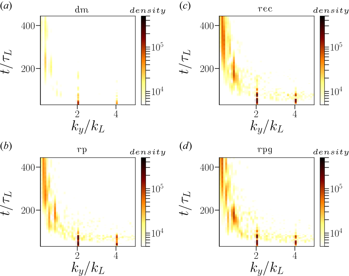
Figure 11. Evolution of the FFT of the ion density oscillations with ($k_y/k_L$ ) for (a) the density modulated target, (b) the rp structured, (c) the rec structured and (d) the rpg structured targets. The modulation parameters are $a_m = 0.25$
 , $k_m = 2$
 and the target width is $d=1.0\lambda _L$
 in each case. The FFT spectra for the flat target is shown in figure 12(a,b). The colorbars represent the density of the FFT spectra, and not the plasma density.
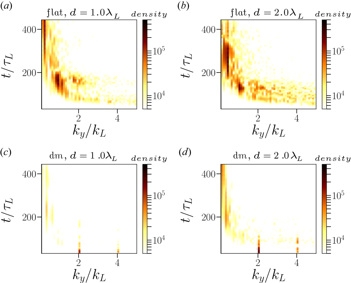
Figure 12. Time development $(t/\tau _L)$ of the FFT of the ion density of a flat target (a,b), and for a density modulated target (c,d) with the normalised wavevector $k_y/k_L$
 . Panels (a,c) and (b,d) are for $d=1.0\lambda _L$
 and $d=2.0\lambda _L$
 target widths in respective cases. The modulation parameters are $a_m = 0.25$
 , $k_m = 2$
 .
.
We follow the same procedure and study the temporal evolution of the FFT of ion density oscillations for density modulated and structured targets for higher $a_0$ cases to see the influence of the RR force on the RPA of ions. In the case of RR force, a significant fraction of the laser energy gets converted into high-energy photons. Consequently the instability that breaks the target becomes only stronger at late-times. Additionally, due to the RR force, bunching of plasma ions is also possible. Since the density modulated targets show better results on the ion acceleration spectra, we compare the cases of a flat target with a density modulated target (corresponding to the best modulation parameters) for $a_0=250$
 and $a_0=350$
 . For the former case, the RR force effects begin to appear in the ion energy spectra. While for the latter case ($a_0=350$
 ), the RR force effects are stronger, but still not requiring us to include the quantum recoil and pair production in PIC simulations. Figure 13 depicts the expected trend as observed before in figure 12. The thinner target ($d=1.0\lambda _L$
 ) shows significant suppression of the long-wavelength mode of the ion density oscillations, while for the thicker target ($d=2.0\lambda _L$
 ) there is indeed an appearance, albeit weaker in magnitude, of the long-wavelength mode. This suggest that eventually the RR force washes out the preimposed modulations in the plasma density and this use of density modulated targets may not be effective for higher $a_0$
 . Indeed this is further confirmed in figure 14 which shows the appearance of strong long-wavelength modes of ion density oscillation being generated at later times. This limits the improvements in the FWHM of ions for the density modulated targets. Though, not shown here, we see similar trends for the other structured targets.

Figure 13. Time development of the FFT of ion density oscillations including RR force for the flat target (a,b) and the density modulated target (c,d) at $a_0=250$ . Panels (a,c) and (b,d) correspond to the target widths of $d=1.0\lambda _L$
 and $d=2.0\lambda _L$
 , respectively. The modulation parameters are $a_m = 0.50, k_m = 2$
 .
.

Figure 14. Time development of the FFT of ion density oscillations including RR force for the flat target (a,b) and the density modulated target (c,d) at $a_0=350$ . Panels (a,c) and (b,d) correspond to the target widths of $d=1.0\lambda _L$
 and $d=2.0\lambda _L$
 , respectively. The modulation parameters are $a_m = 0.50, k_m = 2$
 .
.
Finally, we also carried out 2-D PIC simulations with a laser pulse with Gaussian spatial profile and we recover the same trends as shown before. We show here one simulation run for a target with both density and surface modulations (dm–rpg) and Gaussian shape at the rear end (see figure 15). This target has a spatial density profile, $n(x,y) = n_e a_m [3+\cos (k_m y)]/2$ , and is located between

where $a_c=1.0$ and $b_c=5.0$
 are different dimensionless parameters. The laser pulse has a waist of ${w}=7.0\lambda _L$
 , and $x$
 and $y$
 coordinates of the focus points, $f_x=1.0\lambda _L, f_y=5.0\lambda _L$
 in the simulation box. This combination of density and surface modulations help the target to remain stable in time. The laser pulse can wash out the surface modulations after a while, but as the main target density is also modulated, the laser pulse cannot wash out the density modulations in the early stages (figure 15a). The suppression of long-wavelength modes by competitive feeding is, therefore, most effective for density modulated targets (figure 15c). The Gaussian shape at the rear end of the target in figure 15(b) is necessaryFootnote 2 in order to counter the target breaking caused by the laser pulse with a spatial Gaussian profile (Chen et al. Reference Chen, Pukhov, Yu and Sheng2009). For this simulation, one gets $\Delta E/E_{\textrm {max}} = 17.78\,\%$
 at $t/\tau _L=316$
 with $E_{\textrm {max}}=1.13$
 GeV for a dm target with Gaussian shape at the rear end and $\Delta E/E_{\textrm {max}} = 14.51\,\%$
 at $t/\tau _L=280$
 with $E_{\textrm {max}}=872.33$
 MeV, for an additional surface modulation on top (dm–rpg), incorporated by the cosine term in (3.11) – see figure 16(a). We carried other simulations for different $b_c$
 and $a_c$
 , and the results on the FWHM of the ion energy spectra are depicted in figure 16(b). These results confirm the trends shown before.
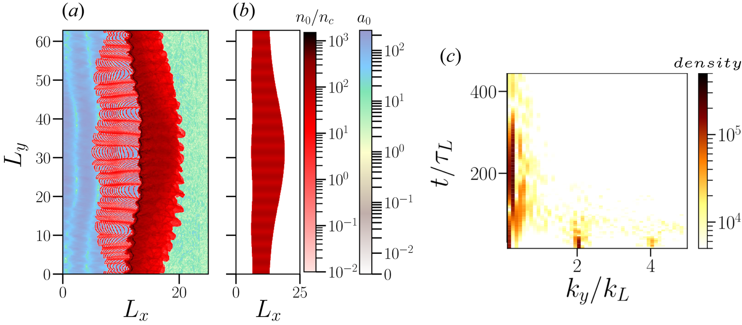
Figure 15. Proton density of a target with dm–rpg. The laser pulse has a spatial Gaussian profile with $a_0=150$ . Panel (a) is at $t/\tau _L=40$
 , while the initial profile at $t/\tau _L=0$
 is shown in (b). (c) Time development of the FFT of the proton density. Modulation parameters are $a_m = 0.25, k_m = 2$
 , and the target widths varies between $d=2.0\lambda _L$
 and $d=1.0\lambda _L$
 (see (3.11)). Moving window velocity is $\upsilon _\textrm {mov} = 0.8\, c$
 .
.
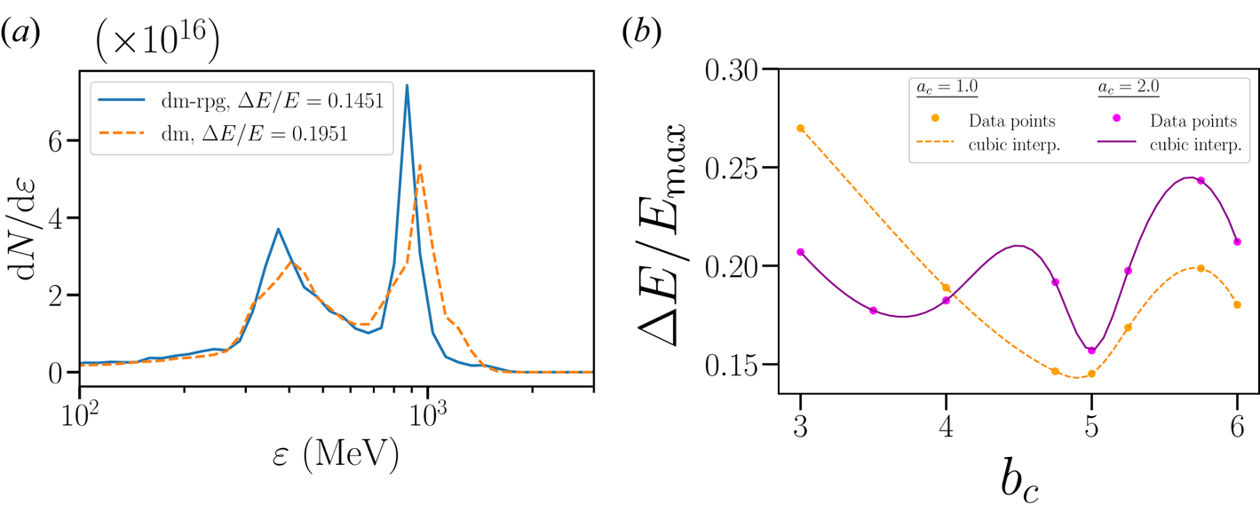
Figure 16. (a) Proton energy spectra corresponding to figure 15(a) at $t/\tau _L =280$ for $a_c=1.0, b_c=5.0$
 . (b) Cubic interpolation of $\Delta E/E_{\textrm {max}}$
 with $b_c$
 and with $a_c=1.0$
 and $a_c=2.0$
 . The other parameters are $a_m = 0.25, k_m = 2, a_0=150$
 .
.
4. Conclusions and discussions
Our 2-D simulation results, especially for the density modulated targets, showing the minimum energy spread ($\Delta E/E_{\textrm {max}} \approx 12\,\%$ ) for 1 GeV protons, are encouraging. Pushing the boundaries of RPA of ions in the radiation dominated regime, one can gain higher proton energies ($E_k \ge 2.0$
 GeV), albeit the FWHM remains stagnant at $\Delta E/E_{\textrm {max}} \sim (12-15)\%$
 . At lower $a_0=250$
 , a thicker target ($d=2.0\lambda _L$
 ) yields better results, while at higher $a_0=350$
 , this trend is reversed with the thinner target ($d=1.0\lambda _L$
 ) showing improved results. Also, the density of accelerated protons is considerably higher at higher $a_0=350$
 . These 2-D simulation results (also with spatial Gaussian laser profile in figure 16) from the density modulated target show substantial enhancements over the flat target case, especially for the FWHM of the proton spectra. This enhancement continues in the radiation dominated regime of proton acceleration. Thus, the improvement in the FWHM for density modulated targets, compared with the flat targets, is robust for the large range of the laser–plasma interaction parameters. The density modulated, as well as structured targets, can be manufactured with newer technological advancements (Klimo et al. Reference Klimo, Psikal, Limpouch, Proska, Novotny, Ceccotti, Floquet and Kawata2011; Fischer & Wegener Reference Fischer and Wegener2013; Cantono et al. Reference Cantono, Permogorov, Ferri, Smetanina, Dmitriev, Persson, Fülöp and Wahlström2021). In particular, it has been shown experimentally that by adjusting the spatial profile of the laser prepulse and introducing a variable delay with the main laser pulse, one can create transient plasma gratings on the surface of the thin-foil target with controllable precision (Monchocé et al. Reference Monchocé, Kahaly, Leblanc, Videau, Combis, Réau, Garzella, D'Oliveira, Martin and Quéré2014). A realistic laser pulse has a long prepulse which ionises the target and creates a preformed plasma in front of the main target. The interaction of prepulse and the rising part of the main laser pulse can also excite, by parametric instabilities, long-wavelength modes of Brillouin instability, which may also have a transverse wavevector associated in a 2-D geometry (Giacone, McKinstrie & Betti Reference Giacone, McKinstrie and Betti1995). This may help in creating the conditions of the density modulated target. For the sake of computational efficiency, we take protons instead of high-Z ions. The results presented here for protons can be recovered for high-$Z$
 ions albeit requiring longer laser pulse durations.
Even though our 2-D simulation results are encouraging, in real experiments 3-D and other physical effects are likely to play a strong role, potentially limiting the ion energy gain and the FWHM of ion energy spectra (Dollar et al. Reference Dollar, Zulick, Thomas, Chvykov, Davis, Kalinchenko, Matsuoka, McGuffey, Petrov and Willingale2012). Some of the geometrical effects related to target bending arising due to the finite laser spot size in a 3-D geometry can be overcome by using the target shapes as studied in figure 15. Further optimisation of the geometry and parameters, for higher ion energy gain in 3-D geometry, can also be undertaken as shown recently (Wang et al. Reference Wang, Khudik and Shvets2021). Nevertheless, results presented here for density modulated targets need to be further explored by taking into account realistic spatiotemporal laser profiles and high-$Z$ targets in 3-D geometry.
Acknowledgements
This work presented here encompasses the bachelor thesis of T.A. Meinhold submitted to the Physics Department of the Heidelberg University.
Editor V. Malka thanks the referees for their advice in evaluating this article.
Supplementary movies
Supplementary movies are available at https://doi.org/10.1017/S0022377821001070.
Declaration of interests
The authors report no conflict of interest.


 Open access