





1. Introduction
Spectral tones are a common feature of both natural and engineering flows, providing valuable insights into the extrinsic and intrinsic, as well as linear and nonlinear, dynamics of fluid systems. These tones appear across a wide range of applications, from engineering systems like turbines and propellers to geophysical flows shaped by planetary motion. While some arise from direct forcing, others emerge intrinsically through hydrodynamic instabilities or resonances. Identifying and distinguishing these spectral features is essential for understanding flow physics, diagnosing instability mechanisms and developing reduced-order models for complex systems.
Fundamental tones either arise from extraneous forcing, or originate from intrinsic flow instabilities or mechanisms. External frequencies are prevalent in many technical applications, such as the blade-passing frequency in rotating machinery like turbines, fans and propellers (Kerwin Reference Kerwin1986; Hansen & Butterfield Reference Hansen and Butterfield1993; Conlisk Reference Conlisk1997; Sandberg & Michelassi Reference Sandberg and Michelassi2022). In geophysical and atmospheric flows, tonal peaks corresponding to semi-diurnal, diurnal and annual frequencies are driven by Earth’s rotation, axial tilt and orbital dynamics relative to the Sun and Moon (Baldwin et al. Reference Baldwin2001; Dijkstra & Burgers Reference Dijkstra and Burgers2002; McWilliams Reference McWilliams2016; Timmermann et al. Reference Timmermann2018). Hydrodynamic instabilities, such as Kelvin–Helmholtz waves in shear-layer flows, represent the second source of fundamental tones. These tones can often be predicted by hydrodynamic stability theory as discrete eigenvalues of the linearised dynamics (Schmid & Henningson Reference Schmid and Henningson2001; Drazin & Reid Reference Drazin and Reid2004). However, even linearly stable flows can exhibit tones when forced near an eigenfrequency, a phenomenon known as linear resonance. Extraneously forced and stable, but non-normal, systems may also undergo pseudoresonance (Trefethen et al. Reference Trefethen, Trefethen, Reddy and Driscoll1993).
Nonlinear tones, on the other hand, arise from the interactions of fundamental or other nonlinear tones. In fluid flows, these originate from the quadratic nonlinearity of the convective term in the Navier–Stokes equations, which generates triadic sum- and difference-frequency and wavenumber interactions (Phillips Reference Phillips1960; Hammack & Henderson Reference Hammack and Henderson1993). Resonant triadic interactions produce peaks at sub-, super- and ultra-harmonic frequencies. They occur in flows with time scales dominated by wave rather than eddy dynamics (Chen et al. Reference Chen, Chen, Eyink and Holm2005; Clark di Leoni & Mininni Reference Clark di Leoni and Mininni2016), and efficiently couple widely disparate time and spatial scales. It is important to distinguish them from non-resonant triadic interactions consisting of compatible frequency or wavenumber triplets that nevertheless do not satisfy the resonant condition. The latter only redistribute energy without producing distinct tones, as seen in the broadband spectrum of isotropic, homogeneous turbulence (Pope Reference Pope2000). While fundamental tones are often straightforward to identify by matching frequencies to known external sources or predictions from linear theory, nonlinear tones are typically identified by matching non-fundamental peaks in power spectra to integer multiples or sums and differences of fundamental frequencies. Since the power spectrum defines energy as the squared magnitude of the signal, it is inherently phase blind. Thus, peaks at sub- and super-harmonic frequencies are a necessary, but not sufficient, condition for confirming nonlinearity (Kim & Powers Reference Kim and Powers1978). The occurrence of ultra-harmonic tones from triadic interactions between different spatial symmetry components adds further complexity to interpreting power spectra alone. The detection of significant nonlinear coupling is therefore predicated on an appropriate measure of the strength of triadic interactions. We will define such a measure, based on statistical correlation, for the analysis of spatio-temporal data.
A well-established tool for identifying triadic interactions in pointwise signals is the bispectrum, along with its normalised counterpart, the bicoherence. The bispectrum is a third-order statistic that correlates two frequency components with their sum, making it useful for detecting triadic frequency interactions that satisfy the zero-sum condition by analysing the phase correlation among the three involved frequencies (see Brillinger (Reference Brillinger1965) for an early review). Building on this, Schmidt (Reference Schmidt2020) proposed bispectral mode decomposition (BMD), which uses an integral measure of bispectral density to identify coherent flow structures associated with triadic interactions. Bispectral mode decomposition achieves this by maximising the integral of the local product of two frequency components and their sum, obtained as the numerical radius of a spectral estimate of the bispectral density matrix. It identifies a single mode pair representing the dominant triad at each point in the bispectrum plane. The method introduced in this work, which we term triadic orthogonal decomposition (TOD), instead maximises the covariance between spectral components, and provides complete, orthogonal bases of convective modes and recipient modes, along with a modal energy budget that quantifies scale-to-scale energy transfer.
While the nonlinear term in the momentum equations can transfer and redistribute kinetic energy, it can neither produce nor remove net energy. The conservation of scale-to-scale kinetic energy transfer has been known at least as far back as the early text of Batchelor (Reference Batchelor1953), and was later expounded on by Kraichnan (Reference Kraichnan1959) in the wavenumber domain. A systematic analysis of spectral energy conservation and transfer was also carried out by Smyth (Reference Smyth1992), which is the foundation for this work. The properties of inter-triad energy conservation are also treated in standard texts, including Lesieur (Reference Lesieur1990), Schmid & Henningson (Reference Schmid and Henningson2001) and others. These properties are directly analogous in the frequency domain. Recent applications of kinetic energy transfer analysis and inter-triad conservation are found in the works of Barthel (Reference Barthel2022) and Freeman, Martinuzzi & Hemmati (Reference Freeman, Martinuzzi and Hemmati2024). The transport of kinetic energy in fluid flows is governed by the dynamical equations for the mean kinetic energy (MKE) and turbulent kinetic energy (TKE). These equations may be partitioned into terms that can be interpreted as distinct mechanisms for energy flow, see e.g. Pope (Reference Pope2000). They include: production, dissipation, advection and the transfer of energy through pressure, viscous diffusion and nonlinear interactions. Depending on the flow, each term represents either a contribution of energy to, or a removal of energy from, the overall kinetic energy budget. In Fourier space, the spectral kinetic energy equation describes the transfer of energy across scales, from frequency to frequency, and wavenumber to wavenumber. One of the pioneering examples of spectral energy-budget analysis of inhomogeneous flows is the work by Lumley (Reference Lumley1964), which investigated the transfer of energy between wavenumbers in wall-bounded turbulence. It proposed the idea of an inverse energy cascade in which energy is transported from smaller to larger scales – a phenomenon now known to be general (Biferale, Musacchio & Toschi Reference Biferale, Musacchio and Toschi2012). Smyth (Reference Smyth1992) later proposed a formalism that enables a systematic examination of the directivity of energy transfer from a donor scale to a recipient scale. Similar observations about energy directivity were also made by Batchelor (Reference Batchelor1953). More recently, the donor–recipient interpretation has been used to study energy transfer in turbulence by Domaradzki & Rogallo (Reference Domaradzki and Rogallo1990), Webber, Handler & Sirovich (Reference Webber, Handler and Sirovich2002), Alexakis et al. (Reference Alexakis, Mininni and Pouquet2005a ), de Wit et al. (Reference de Wit, Aguirre Guzmán, Clercx and Kunnen2022) and Ding, Chung & Illingworth (Reference Ding, Chung and Illingworth2025), as well as in magnetohydrodynamic turbulence by Dar, Verma & Eswaran (Reference Dar, Verma and Eswaran2001) and Alexakis et al. (Reference Alexakis, Mininni and Pouquet2005b ), among others.
Whereas early studies of energy budgets tended to emphasise energy transfer as a local (pointwise) phenomenon, Rempfer & Fasel (Reference Rempfer and Fasel1994) demonstrated that it is possible to incorporate the concept of coherent structures into a framework of modal energy-budget analysis. A comprehensive summary of the methodology and application to a complex bluff-body flow can be found in Hosseini, Martinuzzi & Noack (Reference Hosseini, Martinuzzi and Noack2016). In these works, coherent structures were educed via space-only proper orthogonal decomposition (POD) and employed as the basis for a Galerkin reduced-order model (ROM) of the global energy dynamics. The model thus emphasises the transfer of energy mediated by interactions between structures. Instead of using POD modes, Jin, Symon & Illingworth (Reference Jin, Symon and Illingworth2021) used resolvent modes to compute the convective terms and energy transfers. These modal bases optimally represent the observable dynamics (in the case of POD) or the linear input–output system (in the case of resolvent analysis), with optimality defined in an energy norm. In contrast, TOD by construction explicitly targets individual nonlinear interactions by optimising the covariance between the convective and recipient mode pair for each triad. This feature also makes TOD ideally suited to the analysis of modal energy budgets in the frequency domain. Among the terms in the MKE and TKE budget equations, production, advection and nonlinear transfer are triadic in nature. We show that these triadic energy budgets can be directly recovered from the convective modes and recipient modes of the proposed decomposition.
Instantaneous fluctuating velocities of the three examples considered in § 3 in the $x$
(a,d,g),
$x$
(a,d,g), $y$
(b,e,h) and
$y$
(b,e,h) and $z$
(i) directions: (a,b) cylinder wake; (d,e) wind turbine wake; (g–i) forced isotropic turbulence. Normalised velocity fields (
$z$
(i) directions: (a,b) cylinder wake; (d,e) wind turbine wake; (g–i) forced isotropic turbulence. Normalised velocity fields ( blue, black, red, $q/|\max {\{q\}}|\in [-0.5,0.5 ]$
, with
$q/|\max {\{q\}}|\in [-0.5,0.5 ]$
, with $q$
representing any velocity component) are shown. Area- or volume-integrated power spectra are shown for the cylinder (c), wind turbine (f) and isotropic turbulence (j). In panels (d,e), for clarity the
$q$
representing any velocity component) are shown. Area- or volume-integrated power spectra are shown for the cylinder (c), wind turbine (f) and isotropic turbulence (j). In panels (d,e), for clarity the $x$
- and
$x$
- and $y$
-axes are not drawn to scale. Unless otherwise noted, in what follows, all contours use the same axes limits and colour scales as (a,b) for the cylinder wake, (d,e) for the turbine wake or (g–i) for the isotropic turbulence.
$y$
-axes are not drawn to scale. Unless otherwise noted, in what follows, all contours use the same axes limits and colour scales as (a,b) for the cylinder wake, (d,e) for the turbine wake or (g–i) for the isotropic turbulence.

It is arguably most natural to apply TOD to tonal flows, examples of which were given earlier. Their statistics exhibits a form of sparsity in which the nonlinearity is driven by a subset of all permissible triadic interactions. Indeed, our desire for a systematic approach to studying tonal flows provided the original impetus for this work. The first two applications we present, the wakes of a cylinder and a wind turbine, fall into this category. Their flow fields and power spectra are displayed in the first two rows of figure 1. From visual inspection it is obvious that there are discrete sets of dominant length and time scales, which lock on to each other through the agency of the nonlinear term. Nonetheless, most fluid flows, particularly turbulent ones, are not spectrally sparse. For these flows it is intractable to enumerate all triadic interactions. An archetype of such broadband flows is Kolmogorov turbulence, which provides our third application. Its continuous spectrum is shown in the third row of figure 1. Any description of its dynamics is necessarily incomplete unless all frequencies are considered. Compared with tonal flows, analysing the nonlinearity of broadband flows is thus an acute challenge. However, it is precisely when the number of interactions is large that it becomes imperative to discover patterns in the nonlinearity, whether for physical understanding or model reduction. As our third application demonstrates, for stochastic, broadband flows, TOD yields a ranked decomposition in which each rank in isolation carries clear significance in the context of known physical laws that govern nonlinear interactions – a perhaps surprising finding. The success of TOD in the analysis of both classes of flows, tonal and broadband, as well as laminar and turbulent, testifies to its potential and broad applicability.
The remainder of this paper is organised as follows. First, § 2.1 introduces the governing equations for linear momentum and kinetic energy in the frequency domain and the new orthogonal decomposition. Thereafter, § 2.2 covers the modal energy flow analysis, starting with the theory of the spectral energy budget in § 2.2.1 and inter-triad energy conservation in § 2.2.2, before applying these concepts to modal decomposition in § 2.2.3. Three applications of the decomposition are demonstrated in § 3: the cylinder wake at a Reynolds number of 100 as a canonical example of a nonlinear laminar flow in § 3.1, particle image velocimetry data of a wind turbine wake as an example of a turbulent engineering flow in § 3.2 and three-dimensional numerical simulation data of forced isotropic turbulence as an example of broadband flow in § 3.3. Finally, § 4 discusses our findings and summarises the method.
2. Methods
2.1. Triadic orthogonal decomposition
Throughout this work, we will use the following notational convention: variables which represent scalar-valued functions are italicised, e.g. $q$
; vector-valued functions are italicised and boldface, e.g.
$q$
; vector-valued functions are italicised and boldface, e.g. $\boldsymbol q$
; variables which are spatially discretised vectors are upright and boldface, e.g.
$\boldsymbol q$
; variables which are spatially discretised vectors are upright and boldface, e.g. $\mathbf q$
. We denote the complex conjugate, transpose and Hermitian transpose by the superscripts
$\mathbf q$
. We denote the complex conjugate, transpose and Hermitian transpose by the superscripts $(\boldsymbol{\cdot })^*$
,
$(\boldsymbol{\cdot })^*$
, $(\boldsymbol{\cdot })^{\textrm{T}}$
and
$(\boldsymbol{\cdot })^{\textrm{T}}$
and $(\boldsymbol{\cdot })^{\textrm{H}}$
, respectively. Figure 2 provides a bird’s eye view of the TOD algorithm, which is explained in detail in the following.
$(\boldsymbol{\cdot })^{\textrm{H}}$
, respectively. Figure 2 provides a bird’s eye view of the TOD algorithm, which is explained in detail in the following.
The TOD algorithm. The top row provides a graphical representation of the matrix algebra, while the bottom row illustrates the algorithm using a cylinder wake dataset. In this example, the convective and recipient modes are similar to the convective and recipient fields because the cylinder wake is laminar and periodic. Key equations are referenced by number. SVD stands for the singular value decomposition.

2.1.1. Spectral momentum and kinetic energy equations
The motion of an incompressible Newtonian fluid is governed by the momentum and continuity equations
 \begin{align} \frac {\partial \boldsymbol{u}}{\partial t} &= -(\boldsymbol u\boldsymbol{\cdot }\boldsymbol{\nabla })\boldsymbol u - \boldsymbol{\nabla }\!p + \frac {1}{\textit{Re}}{\nabla} ^2\boldsymbol u, \end{align}
 \begin{align} \boldsymbol{\nabla }\boldsymbol{\cdot }\boldsymbol u&=0, \end{align}
where $\boldsymbol u = [u\;v\;w]^{\textrm{T}}$
is the velocity vector field and
$\boldsymbol u = [u\;v\;w]^{\textrm{T}}$
is the velocity vector field and $p$
is the pressure field. Equation (2.1a
) has been non-dimensionalised by the velocity scale,
$p$
is the pressure field. Equation (2.1a
) has been non-dimensionalised by the velocity scale, $U_\infty$
, the length scale,
$U_\infty$
, the length scale, $L$
and is parameterised by the Reynolds number,
$L$
and is parameterised by the Reynolds number, $Re= {U_\infty L}/{\nu }$
, where
$Re= {U_\infty L}/{\nu }$
, where $\nu$
is the kinematic viscosity. Assuming a time-periodic flow, the flow variables can be expanded as the Fourier series
$\nu$
is the kinematic viscosity. Assuming a time-periodic flow, the flow variables can be expanded as the Fourier series
 \begin{align} \boldsymbol u(\boldsymbol x,t) = \sum _{n=-\infty }^\infty \hat {\boldsymbol u}_n(\boldsymbol x)\textrm{e}^{\textrm{i} 2\pi f_n t} \quad \textrm{and}\quad p(\boldsymbol x,t) = \sum _{n=-\infty }^\infty \hat {p}_n(\boldsymbol x)\textrm{e}^{\textrm{i} 2\pi f_n t}. \end{align}
For each frequency, $f_n$
, we obtain the frequency-domain representation of (2.1a)
$f_n$
, we obtain the frequency-domain representation of (2.1a)
 \begin{align} \textrm{i} 2\pi f_n \hat {\boldsymbol u}_n &= -\left (\widehat {(\boldsymbol u\boldsymbol{\cdot }\boldsymbol{\nabla })\boldsymbol u}\right )_n - \boldsymbol{\nabla }\!\hat {p}_n + \frac {1}{\textit{Re}}{\nabla} ^2\hat {\boldsymbol u}_n = -\sum _{l=-\infty }^\infty \underbrace {(\hat {\boldsymbol u}_{n-l}\boldsymbol{\cdot }\boldsymbol{\nabla })\hat {\boldsymbol u}_l}_{-\boldsymbol{\hat {c}}_{l\rightarrow n}} - \boldsymbol{\nabla }\!\hat {p}_n + \frac {1}{\textit{Re}}{\nabla} ^2\hat {\boldsymbol u}_n , \end{align}
where, in the second step, we have invoked the convolution theorem. This frequency-domain, or spectral, momentum equation lies at the core of our modal momentum transfer analysis. The special role and implications of the components in the convolution sum, $\boldsymbol{\hat {c}}_{l\rightarrow n}$
, are discussed in § 2.1.2.
$\boldsymbol{\hat {c}}_{l\rightarrow n}$
, are discussed in § 2.1.2.
For the often-used notation of triads, $(k,l,n)$
with
$(k,l,n)$
with $k=n-l$
, any two of the frequency components determine the remaining one. For simplicity, we use the pairwise notation
$k=n-l$
, any two of the frequency components determine the remaining one. For simplicity, we use the pairwise notation $(l,n)$
to denote the triplet
$(l,n)$
to denote the triplet $(n-l,l,n)$
in the following. For the case of
$(n-l,l,n)$
in the following. For the case of $n=0$
, (2.3) simplifies to
$n=0$
, (2.3) simplifies to
 \begin{align} 0 &= -(\bar {\boldsymbol u}\boldsymbol{\cdot }\boldsymbol{\nabla })\bar {\boldsymbol u} -\sum _{l\neq 0} \underbrace {(\hat {\boldsymbol u}_{-l}\boldsymbol{\cdot }\boldsymbol{\nabla })\hat {\boldsymbol u}_l}_{-\boldsymbol{\hat {c}}_{l\rightarrow 0}} - \boldsymbol{\nabla }\bar {p} + \frac {1}{\textit{Re}}{\nabla} ^2\bar {\boldsymbol u} \nonumber\\&= -(\bar {\boldsymbol u}\boldsymbol{\cdot }\boldsymbol{\nabla })\bar {\boldsymbol u} - \overline {(\boldsymbol u'\boldsymbol{\cdot }\boldsymbol{\nabla })\boldsymbol u'} - \boldsymbol{\nabla }\bar {p} + \frac {1}{\textit{Re}}{\nabla} ^2\bar {\boldsymbol u}, \end{align}
which are the Reynolds-averaged Navier–Stokes (RANS) equations, with $\boldsymbol u'\equiv \boldsymbol u{-}\bar {\boldsymbol u}$
. The definition of
$\boldsymbol u'\equiv \boldsymbol u{-}\bar {\boldsymbol u}$
. The definition of $\boldsymbol u'$
implies that
$\boldsymbol u'$
implies that $\hat {\boldsymbol u}_l=\widehat {\boldsymbol u'_l}$
for
$\hat {\boldsymbol u}_l=\widehat {\boldsymbol u'_l}$
for $l\neq 0$
, which leads to the second equality in (2.4). Each term in the RANS equations contributes to the deformation of the mean flow,
$l\neq 0$
, which leads to the second equality in (2.4). Each term in the RANS equations contributes to the deformation of the mean flow, $\bar {\boldsymbol u}$
. The term
$\bar {\boldsymbol u}$
. The term $\boldsymbol{\hat {c}}_{l\rightarrow 0}$
, in particular, is responsible for momentum transfer via the Reynolds stress,
$\boldsymbol{\hat {c}}_{l\rightarrow 0}$
, in particular, is responsible for momentum transfer via the Reynolds stress, $\overline {(\boldsymbol u'\boldsymbol{\cdot }\boldsymbol{\nabla })\boldsymbol u'}$
.
$\overline {(\boldsymbol u'\boldsymbol{\cdot }\boldsymbol{\nabla })\boldsymbol u'}$
.
Upon left-multiplying with $\hat {\boldsymbol u}_n^{\textrm{H}}$
, (2.3) can be rewritten as the spectral kinetic energy equation
$\hat {\boldsymbol u}_n^{\textrm{H}}$
, (2.3) can be rewritten as the spectral kinetic energy equation
 \begin{align} \textrm{i} 2\pi f_n\hat {\boldsymbol u}_n^{\textrm{H}}\hat {\boldsymbol u}_n = -\hat {\boldsymbol u}_n^{\textrm{H}}\sum _{l=-\infty }^\infty \underbrace {(\hat {\boldsymbol u}_{n-l}\boldsymbol{\cdot }\boldsymbol{\nabla })\hat {\boldsymbol u}_l}_{-\boldsymbol{\hat {c}}_{l\rightarrow n}} - \boldsymbol{\nabla }\boldsymbol{\cdot }\left(\hat {p}_n\hat {\boldsymbol u}_n^{\textrm{H}}\right) + \frac {1}{\textit{Re}}\hat {\boldsymbol u}_n^{\textrm{H}}{\nabla} ^2\hat {\boldsymbol u}_n. \end{align}
The spectral kinetic energy equation governs the distribution of the kinetic energy, $\hat {E}_n= {1}/{2}(\hat {\boldsymbol u}_n^{\textrm{H}}\hat {\boldsymbol u}_n)$
, and forms the basis for the modal energy flow analysis in § 2.2. A remarkable property of (2.5) regarding the convective term, which is not used here but discussed in detail by Freeman et al. (Reference Freeman, Martinuzzi and Hemmati2024), is that, under certain conditions, the imaginary part of the term can be used to recover the integral power of the velocity, and the real part the integral dissipation.
$\hat {E}_n= {1}/{2}(\hat {\boldsymbol u}_n^{\textrm{H}}\hat {\boldsymbol u}_n)$
, and forms the basis for the modal energy flow analysis in § 2.2. A remarkable property of (2.5) regarding the convective term, which is not used here but discussed in detail by Freeman et al. (Reference Freeman, Martinuzzi and Hemmati2024), is that, under certain conditions, the imaginary part of the term can be used to recover the integral power of the velocity, and the real part the integral dissipation.
A wide variety of open flows exhibit strong convective instability. Examples encompass natural and technical flows, such as bluff-body wakes and boundary layers, as well as exogenously forced flows like plasma-actuated jets. In these flows, the convective term $\boldsymbol{\hat {c}}_{l\rightarrow n}$
becomes dominant in both spectral momentum and kinetic energy equations. In the following, we outline how the spatial structures involved in spectral momentum transfer can be leveraged to identify and understand triadic flow interactions.
$\boldsymbol{\hat {c}}_{l\rightarrow n}$
becomes dominant in both spectral momentum and kinetic energy equations. In the following, we outline how the spatial structures involved in spectral momentum transfer can be leveraged to identify and understand triadic flow interactions.
2.1.2. Recipient–donor framework
The recipient–donor framework (Batchelor Reference Batchelor1953; Smyth Reference Smyth1992) of the momentum equations is a key concept that facilitates the calculation of both the direction and magnitude of modal energy transfer. In (2.3), we introduced the notation
 \begin{equation} \boldsymbol{\hat {c}}_{l\rightarrow n} = -(\hat {\boldsymbol u}_{n-l}\boldsymbol{\cdot }\boldsymbol{\nabla })\hat {\boldsymbol u}_l \end{equation}
to represent the component in the convolution sum associated with the frequency pair $(l,n)$
, or the corresponding triplet
$(l,n)$
, or the corresponding triplet $(n-l,l,n)$
. This notation implicitly denotes the direction of momentum transfer,
$(n-l,l,n)$
. This notation implicitly denotes the direction of momentum transfer, $l\rightarrow n$
, from frequency component
$l\rightarrow n$
, from frequency component $\hat {\boldsymbol u}_l$
to
$\hat {\boldsymbol u}_l$
to $\hat {\boldsymbol u}_n$
. As (2.3) governs the velocity component at frequency
$\hat {\boldsymbol u}_n$
. As (2.3) governs the velocity component at frequency $f_n$
, we denote the component
$f_n$
, we denote the component $\hat {\boldsymbol u}_n$
as the recipient of linear momentum (although contributions can be negative, resulting in a net loss of momentum). We first present an intuitive argument based on the roles of
$\hat {\boldsymbol u}_n$
as the recipient of linear momentum (although contributions can be negative, resulting in a net loss of momentum). We first present an intuitive argument based on the roles of $\hat {\boldsymbol u}_{n-l}$
and
$\hat {\boldsymbol u}_{n-l}$
and $\hat {\boldsymbol u}_l$
in
$\hat {\boldsymbol u}_l$
in $\boldsymbol{\hat {c}}_{l\rightarrow n}$
in the familiar derivation of the momentum equations, which indicates that the velocity component
$\boldsymbol{\hat {c}}_{l\rightarrow n}$
in the familiar derivation of the momentum equations, which indicates that the velocity component $\hat {\boldsymbol u}_{n-l}$
advects
$\hat {\boldsymbol u}_{n-l}$
advects $\hat {\boldsymbol u}_l$
in the direction of, and with a magnitude proportional to, its gradient field,
$\hat {\boldsymbol u}_l$
in the direction of, and with a magnitude proportional to, its gradient field, $\boldsymbol{\nabla }\hat {\boldsymbol u}_l$
. Thus
$\boldsymbol{\nabla }\hat {\boldsymbol u}_l$
. Thus $\hat {\boldsymbol u}_l$
serves as a donor of linear momentum to
$\hat {\boldsymbol u}_l$
serves as a donor of linear momentum to $\hat {\boldsymbol u}_n$
, while
$\hat {\boldsymbol u}_n$
, while $\hat {\boldsymbol u}_{n-l}$
acts as the passive advector. To avoid confusion with the convective field,
$\hat {\boldsymbol u}_{n-l}$
acts as the passive advector. To avoid confusion with the convective field, $\boldsymbol{\hat {c}}_{l\rightarrow n}$
, which ultimately contributes to
$\boldsymbol{\hat {c}}_{l\rightarrow n}$
, which ultimately contributes to $\hat {\boldsymbol u}_n$
and hence frequency
$\hat {\boldsymbol u}_n$
and hence frequency $f_{n}$
, we refer to
$f_{n}$
, we refer to $\hat {\boldsymbol u}_{n-l}$
as the catalyst field, and
$\hat {\boldsymbol u}_{n-l}$
as the catalyst field, and $f_{n-l}$
as the catalyst frequency.
$f_{n-l}$
as the catalyst frequency.
From the derivation and final form of (2.5), which governs the spectral kinetic energy $\hat {E}_n= {1}/{2}(\hat {\boldsymbol u}_n^{\textrm{H}}\hat {\boldsymbol u}_n)$
, it is evident that spectral energy transfer to frequency
$\hat {E}_n= {1}/{2}(\hat {\boldsymbol u}_n^{\textrm{H}}\hat {\boldsymbol u}_n)$
, it is evident that spectral energy transfer to frequency $f_{n}$
results directly from momentum transfer by the convective field,
$f_{n}$
results directly from momentum transfer by the convective field, $\boldsymbol{\hat {c}}_{l\rightarrow n}$
. The donor–recipient interpretation from
$\boldsymbol{\hat {c}}_{l\rightarrow n}$
. The donor–recipient interpretation from $f_{l}$
to
$f_{l}$
to $f_{n}$
therefore directly translates to the transfer of energy, and can, in fact, be derived from the inter-triad energy conservation discussed in § 2.2.2. Specifically, under certain conditions, the energy transfer by triad
$f_{n}$
therefore directly translates to the transfer of energy, and can, in fact, be derived from the inter-triad energy conservation discussed in § 2.2.2. Specifically, under certain conditions, the energy transfer by triad $(n-l,l,n)$
is exactly equal and opposite to that by the triad
$(n-l,l,n)$
is exactly equal and opposite to that by the triad $(l-n,n,l)$
and hence independent of the catalyst component. This second, rigorous motivation of the recipient–donor interpretation is elaborated on in § 2.2.3.
$(l-n,n,l)$
and hence independent of the catalyst component. This second, rigorous motivation of the recipient–donor interpretation is elaborated on in § 2.2.3.
2.1.3. Modal decomposition
The recipient–donor interpretation of the spectral momentum and kinetic energy equations, as summarised in § 2.1.2, establishes the relationship where $\hat {\boldsymbol u}_n$
acts as the recipient of momentum or energy through the action of the convective field,
$\hat {\boldsymbol u}_n$
acts as the recipient of momentum or energy through the action of the convective field, $\boldsymbol{\hat {c}}_{l\rightarrow n}$
. The objective of the decomposition is to identify the flow structures that, on average, contribute most to the momentum transfer. This objective can be framed as an optimisation problem using the calculus of variations, where a pair of jointly optimal modal bases for a given triad,
$\boldsymbol{\hat {c}}_{l\rightarrow n}$
. The objective of the decomposition is to identify the flow structures that, on average, contribute most to the momentum transfer. This objective can be framed as an optimisation problem using the calculus of variations, where a pair of jointly optimal modal bases for a given triad, $(l,n)$
, are computed such that the convective term,
$(l,n)$
, are computed such that the convective term, $\boldsymbol{\hat {c}}_{l\to n}$
, and the recipient,
$\boldsymbol{\hat {c}}_{l\to n}$
, and the recipient, $\boldsymbol{\hat {u}}_{n}$
, are optimally represented in terms of their covariance. The kinetic energy of the convective term and the recipient are measured in the norm
$\boldsymbol{\hat {u}}_{n}$
, are optimally represented in terms of their covariance. The kinetic energy of the convective term and the recipient are measured in the norm $\|\boldsymbol{\cdot }\|$
, induced by the inner product
$\|\boldsymbol{\cdot }\|$
, induced by the inner product
 \begin{equation} \langle {\boldsymbol u_1(\boldsymbol{x}),\boldsymbol u_2(\boldsymbol{x})\rangle } = \int _{\varOmega } \boldsymbol u_2^{\textrm{H}}(\boldsymbol{x}) \boldsymbol u_1(\boldsymbol{x}) \, \textrm{d} \boldsymbol{x}. \end{equation}
The optimal convective–recipient covariance for each donor–recipient pair, $\sigma (l,n)\in \mathbb{R}_{\geq 0}$
, is given by the optimisation problem
$\sigma (l,n)\in \mathbb{R}_{\geq 0}$
, is given by the optimisation problem
 \begin{align} \sigma (l,n) & = \max \frac {{E}\left \{ \langle { \boldsymbol{\hat {c}}_{l\to n}(\boldsymbol{x}),\boldsymbol{\hat {\psi }}_{l\to n}(\boldsymbol{x})\rangle } \langle {\boldsymbol{\hat {u}}_{n}(\boldsymbol{x}'),\boldsymbol{\hat {\phi }}_{n}(\boldsymbol{x}')\rangle }^* \right \}}{ \|{ \boldsymbol{\hat {\psi }}_{l\to n}(\boldsymbol{x})\|} \|{\boldsymbol{\hat {\phi }}_n(\boldsymbol{x}')\|} } \end{align}
 \begin{align} & = \max \frac {{E}\left \{ \left (\int _{\varOmega } \boldsymbol{\hat {\psi }}_{l\to n}^{\textrm{H}}(\boldsymbol{x}) \boldsymbol{\hat {c}}_{l\to n}(\boldsymbol{x}) \, \textrm{d} \boldsymbol{x} \right )\left ( \int _{\varOmega } \boldsymbol{\hat {u}}_{n}^{\textrm{H}}(\boldsymbol{x}') \boldsymbol{\hat {\phi }}_{n}(\boldsymbol{x}') \, \textrm{d} \boldsymbol{x}' \right ) \right \}}{ \|{ \boldsymbol{\hat {\psi }}_{l\to n}(\boldsymbol{x})\|} \|{\boldsymbol{\hat {\phi }}_n(\boldsymbol{x}')\|} } \end{align}
 \begin{align} & = \max \frac {{E}\left \{ \iint _{\varOmega } \boldsymbol{\hat {\psi }}_{l\to n}^{\textrm{H}}(\boldsymbol{x}) \left ( \boldsymbol{\hat {c}}_{l\to n}(\boldsymbol{x}) \boldsymbol{\hat {u}}^{\textrm{H}}_{n}(\boldsymbol{x}') \right ) \boldsymbol{\hat {\phi }}_{n}(\boldsymbol{x}') \, \textrm{d} \boldsymbol{x} \, \textrm{d} \boldsymbol{x}' \right \}}{ \|{ \boldsymbol{\hat {\psi }}_{l\to n}(\boldsymbol{x})\|} \|{\boldsymbol{\hat {\phi }}_n(\boldsymbol{x}')\|} } \end{align}
 \begin{align} & = \max \frac { \iint _{\varOmega } \boldsymbol{\hat {\psi }}_{l\to n}^{\textrm{H}}(\boldsymbol{x}) \boldsymbol{S}(\boldsymbol x,\boldsymbol x';n,l) \boldsymbol{\hat {\phi }}_{n}(\boldsymbol{x}') \, \textrm{d} \boldsymbol{x} \, \textrm{d} \boldsymbol{x}' }{ \|{ \boldsymbol{\hat {\psi }}_{l\to n}(\boldsymbol{x})\|} \|{\boldsymbol{\hat {\phi }}_n(\boldsymbol{x}')\|} }, \end{align}
where
 \begin{align} \boldsymbol{S}(\boldsymbol x,\boldsymbol x';l,n) = {E}\left \{\boldsymbol{\hat {c}}_{l\to n}(\boldsymbol x)\boldsymbol{\hat {u}}^{\textrm{H}}_{n}(\boldsymbol x')\right \} \end{align}
represents the two-point cross-bispectral covariance tensor. This tensor is a Fredholm kernel, and the modes that jointly maximise $\sigma$
can be obtained via the singular value expansion (SVE) of
$\sigma$
can be obtained via the singular value expansion (SVE) of $\boldsymbol{S}$
(Schmidt Reference Schmidt1907), that is
$\boldsymbol{S}$
(Schmidt Reference Schmidt1907), that is
 \begin{align} \boldsymbol{S}(\boldsymbol x,\boldsymbol x';l,n) = \sum _{j=1}^{\infty } \sigma _{\!j} { \boldsymbol{\hat {\psi }}}_{l\to n,j}(\boldsymbol{x})\boldsymbol{\hat {\phi }}^{\textrm{H}}_{n,j}(\boldsymbol{x}'). \end{align}
The reality and non-negativeness of $\sigma$
are guaranteed by the SVE. The convective mode,
$\sigma$
are guaranteed by the SVE. The convective mode, $ \boldsymbol{\hat {\psi }}_{l\to n,j}$
, and recipient mode,
$ \boldsymbol{\hat {\psi }}_{l\to n,j}$
, and recipient mode, $\boldsymbol{\hat {\phi }}_{n,j}$
, are ordered by their associated singular values,
$\boldsymbol{\hat {\phi }}_{n,j}$
, are ordered by their associated singular values, ${\sigma _1}\geqslant {\sigma _2}\geqslant {\cdots} \geqslant 0$
. They are also orthogonal in their respective inner products and have unit energy, that is,
${\sigma _1}\geqslant {\sigma _2}\geqslant {\cdots} \geqslant 0$
. They are also orthogonal in their respective inner products and have unit energy, that is, $\left \langle \boldsymbol{\hat {\psi }}_{l\to n,i}, \boldsymbol{\hat {\psi }}_{l\to n,j}\right \rangle = \left \langle \boldsymbol{\hat {\phi }}_{n,i},\boldsymbol{\hat {\phi }}_{n,j}\right \rangle =\delta _{ij}$
. In practice, that is for discrete data, (2.10) is solved by the singular value decomposition. In the special case where the convective term is identical to the recipient,
$\left \langle \boldsymbol{\hat {\psi }}_{l\to n,i}, \boldsymbol{\hat {\psi }}_{l\to n,j}\right \rangle = \left \langle \boldsymbol{\hat {\phi }}_{n,i},\boldsymbol{\hat {\phi }}_{n,j}\right \rangle =\delta _{ij}$
. In practice, that is for discrete data, (2.10) is solved by the singular value decomposition. In the special case where the convective term is identical to the recipient, $\boldsymbol{\hat {c}}_{l\to n}= \boldsymbol{\hat {u}}_{n}$
, (2.8)–(2.10) reduce to the POD framework by Lumley (Reference Lumley1967, Reference Lumley1970). By defining the expansion coefficients as the projections of the convective term and the recipient onto their respective modal bases (suppressing their dependence on
$\boldsymbol{\hat {c}}_{l\to n}= \boldsymbol{\hat {u}}_{n}$
, (2.8)–(2.10) reduce to the POD framework by Lumley (Reference Lumley1967, Reference Lumley1970). By defining the expansion coefficients as the projections of the convective term and the recipient onto their respective modal bases (suppressing their dependence on $l$
and
$l$
and $n$
for clarity),
$n$
for clarity),
 \begin{align} a_{\!j} = \left \langle \boldsymbol{\hat {u}}_{n},\boldsymbol{\hat {\phi }}_{n,j}\right \rangle \quad \textrm{and} \quad b_{\!j} = \left \langle \boldsymbol{\hat {c}}_{l\to n},\boldsymbol{\hat {\psi }}_{l\to n,j}\right \rangle , \end{align}
we obtain the jointly optimal, ranked decomposition,
 \begin{align} \boldsymbol{\hat {u}}_{n} = \sum _{j= 1}^{\infty } a_{\!j} \boldsymbol{\hat {\phi }}_{n,j} \quad \textrm{and} \quad \boldsymbol{\hat {c}}_{l\to n}= \sum _{j= 1}^{\infty } b_{\!j} \boldsymbol{\hat {\psi }}_{l\to n,j}. \end{align}
The expansion coefficients, $a$
and
$a$
and $b$
, satisfy
$b$
, satisfy
 \begin{equation} {E}\{ b_{\!j} a_k^{*} \} = \sigma _{\!j} \delta _{jk}. \end{equation}
In other words, the coefficients are uncorrelated with one another. Since the coefficients are complex quantities that retain phase information, the covariance between $a_{\!j}$
and
$a_{\!j}$
and $b_{\!j}$
, i.e. the singular value, additionally measures the degree of phase coupling between the projections of the recipient,
$b_{\!j}$
, i.e. the singular value, additionally measures the degree of phase coupling between the projections of the recipient, $\boldsymbol{\hat {u}}_{n}$
, and the convective term,
$\boldsymbol{\hat {u}}_{n}$
, and the convective term, $\boldsymbol{\hat {c}}_{l\to n}$
.
$\boldsymbol{\hat {c}}_{l\to n}$
.
The expansion coefficients are also a convenient means to retrieve the spectral energy distribution of the velocity. From the mutual orthogonality of the modes, it is easily shown that the velocity power spectrum, ${E}\{\|{\hat {\boldsymbol u}_n}\|^2\}$
, is recovered from the sum of the squared recipient mode coefficients
${E}\{\|{\hat {\boldsymbol u}_n}\|^2\}$
, is recovered from the sum of the squared recipient mode coefficients
 \begin{equation} {E}\bigl\{\|{\hat {\boldsymbol u}_n}\|^2\bigr\} = \sum _{j=1}^\infty {E}\bigl\{a_{\!j}a_{\!j}^*\bigr\}. \end{equation}
Equation (2.14) holds for any triad $(l,n)$
and indicates that the total power spectrum can be decomposed into contributions from individual modal ranks. The power spectra previously shown in figure 1 are obtained using this equality.
$(l,n)$
and indicates that the total power spectrum can be decomposed into contributions from individual modal ranks. The power spectra previously shown in figure 1 are obtained using this equality.
To obtain convergent estimates of the bispectral densities, we adapt Welch’s method (Welch Reference Welch1967) in the decomposition framework to construct an ensemble of realisations of the temporal Fourier transform of the data from a single time series consisting of $N_t$
snapshots based on the ergodicity hypothesis for statistically stationary flows. First, the data are segmented into
$N_t$
snapshots based on the ergodicity hypothesis for statistically stationary flows. First, the data are segmented into $N_{\textit{blk}}$
(potentially overlapping by
$N_{\textit{blk}}$
(potentially overlapping by $N_{\textit{ovlp}}$
snapshots) blocks containing
$N_{\textit{ovlp}}$
snapshots) blocks containing $N_{\!f}$
consecutive snapshots separated by time step
$N_{\!f}$
consecutive snapshots separated by time step $\Delta t$
. Each snapshot is represented by a column vector of length
$\Delta t$
. Each snapshot is represented by a column vector of length $N$
, corresponding to the number of spatial degrees of freedom times the number of velocity components, i.e. the dimension of the data. The
$N$
, corresponding to the number of spatial degrees of freedom times the number of velocity components, i.e. the dimension of the data. The $m$
th block is defined as
$m$
th block is defined as
 \begin{align} \mathbf{U}^{(m)} &= \left [ \begin{matrix} \mathbf{u}_{1}^{(m)}& \mathbf{u}_{2}^{(m)} &{\cdots} & \mathbf{u}_{N_{\!f}}^{(m)} \end{matrix}\right ] \in \mathbb{C}^{N\times N_{\!f}}, \end{align}
and its temporal, i.e. row-wise, discrete Fourier transform (DFT) is denoted by
 \begin{align} {\hat {\mathbf{U}}}^{(m)} &= \left [ \begin{matrix} {\hat {\mathbf{u}}}_{1}^{(m)}& {\hat {\mathbf{u}}}_{2}^{(m)} &{\cdots} & {\hat {\mathbf{u}}}_{N_{\!f}}^{(m)} \end{matrix}\right ]. \end{align}
This is the same spectral estimation technique commonly used in spectral proper orthogonal decomposition (SPOD), and readers are referred to Towne, Schmidt & Colonius (Reference Towne, Schmidt and Colonius2018) and Schmidt & Colonius (Reference Schmidt and Colonius2020) for more details and best practices. Next, the data matrices for the recipient and convective terms
 \begin{align} {\hat {\mathbf{U}}}_{n} &= \left [ \begin{matrix} {\hat {\mathbf{u}}}_{n}^{(1)}& {\hat {\mathbf{u}}}_{n}^{(2)} &{\cdots} & {\hat {\mathbf{u}}}_{n}^{(N_{\textit{blk}})} \end{matrix}\right ], \end{align}
 \begin{align} {\hat {\mathbf{C}}}_{l\to n} &= \left [ \begin{matrix} {\hat {\mathbf{c}}}_{l\to n}^{(1)} & {\hat {\mathbf{c}}}_{l\to n}^{(2)} & {\cdots} & {\hat {\mathbf{c}}}_{l\to n}^{(N_{\textit{blk}})} \end{matrix}\right ] \nonumber \\ &= -\left [ \begin{matrix} \left({\hat {\mathbf{u}}}_{n-l}^{(1)}\boldsymbol{\cdot }\boldsymbol{\nabla }\right)\hat {\mathbf{u}}_l^{(1)} & \left(\hat {\mathbf{u}}_{n-l}^{(2)}\boldsymbol{\cdot }\boldsymbol{\nabla }\right)\hat {\mathbf{u}}_l^{(2)} & {\cdots} &\left(\hat {\mathbf{u}}_{n-l}^{(N_{\textit{blk}})}\boldsymbol{\cdot }\boldsymbol{\nabla }\right)\hat {\mathbf{u}}_l^{(N_{\textit{blk}})} \end{matrix}\right ]\!, \end{align}
are assembled from the columns of ${\hat {\mathbf{U}}}^{(m)}$
. Then, the two-point cross-bispectral covariance tensor at triad
${\hat {\mathbf{U}}}^{(m)}$
. Then, the two-point cross-bispectral covariance tensor at triad $(l,n)$
can be approximated as
$(l,n)$
can be approximated as
 \begin{align} {\mathbf{S}}_{l,n} = {\frac {1}{N_{\textit{blk}}}}{\hat {\mathbf{C}}}_{l\to n} {\hat {\mathbf{U}}}_{n}^{\mathrm{H}}. \end{align}
Using this approximation, the infinite-dimensional SVE problem in (2.10) reduces to an $N\times N$
matrix SVD problem
$N\times N$
matrix SVD problem
 \begin{align} {\mathbf{W}}^{1/2}{\mathbf{S}}_{l,n}{\mathbf{W}}^{1/2} &= {\boldsymbol{\tilde {\Psi }}}_{l\to n}{\boldsymbol{\Sigma }}_{l\to n}\boldsymbol{\tilde {\Phi }}_{n}^{\mathrm{H}}, \end{align}
for the convective–recipient covariances, $\boldsymbol{\Sigma }_{l,n}=\textrm{diag}([\sigma _1, \sigma _2, \ldots , \sigma _{N_{\textit{blk}}}])$
, captured by each mode pair. The convective and recipient modes can be recovered as
$\boldsymbol{\Sigma }_{l,n}=\textrm{diag}([\sigma _1, \sigma _2, \ldots , \sigma _{N_{\textit{blk}}}])$
, captured by each mode pair. The convective and recipient modes can be recovered as
 \begin{align} \boldsymbol{\hat {\Psi }}_{l\to n} ={\mathbf{W}}^{-1/2} \boldsymbol{\tilde {\Psi }}_{l\to n} \quad \textrm{and}\quad \boldsymbol{\hat {\Phi }}_{n} = {\mathbf{W}}^{-1/2}\boldsymbol{\tilde {\Phi }}_{n}, \end{align}
respectively, and ${\mathbf {W}}$
is a weight matrix that accounts for the quadrature weights. In practice, there is no need to directly solve this SVD problem as the matrix
${\mathbf {W}}$
is a weight matrix that accounts for the quadrature weights. In practice, there is no need to directly solve this SVD problem as the matrix ${\mathbf{S}}$
is low-rank with a rank of
${\mathbf{S}}$
is low-rank with a rank of $N_{\textit{blk}}\ll N$
. Instead, we first perform the QR decomposition of the weighted convective term data matrix
$N_{\textit{blk}}\ll N$
. Instead, we first perform the QR decomposition of the weighted convective term data matrix
 \begin{align} \frac {1}{N_{\textit{blk}}}{{\mathbf{W}}^{1/2}}{\hat {\mathbf{C}}}_{l\to n} = {\mathbf{C}}_\perp {\mathbf{C}}_\triangle , \end{align}
where ${\mathbf{C}}_\perp \in \mathbb{C}^{N\times N_{\textit{blk}}}$
is orthonormal and
${\mathbf{C}}_\perp \in \mathbb{C}^{N\times N_{\textit{blk}}}$
is orthonormal and ${\mathbf{C}}_\triangle \in \mathbb{C}^{N_{\textit{blk}}\times N_{\textit{blk}}}$
is upper triangular. We then compute the eigenvalue decomposition of the Hermitian matrix
${\mathbf{C}}_\triangle \in \mathbb{C}^{N_{\textit{blk}}\times N_{\textit{blk}}}$
is upper triangular. We then compute the eigenvalue decomposition of the Hermitian matrix ${\mathbf{C}}_\triangle {\hat {\mathbf{U}}}_{n}^{\mathrm{H}} {\mathbf{W}} {\hat {\mathbf{U}}}_{n} {\mathbf{C}}_\triangle ^{\mathrm{H}} \in \mathbb{C}^{N_{\textit{blk}}\times N_{\textit{blk}}}$
such that
${\mathbf{C}}_\triangle {\hat {\mathbf{U}}}_{n}^{\mathrm{H}} {\mathbf{W}} {\hat {\mathbf{U}}}_{n} {\mathbf{C}}_\triangle ^{\mathrm{H}} \in \mathbb{C}^{N_{\textit{blk}}\times N_{\textit{blk}}}$
such that
 \begin{align} \left ({\mathbf{C}}_\triangle {\hat {\mathbf{U}}}_{n}^{\mathrm{H}} {\mathbf{W}} {\hat {\mathbf{U}}}_{n} {\mathbf{C}}_\triangle ^{\mathrm{H}}\right ){\boldsymbol{{\Psi }}_{l\to n}} = {\boldsymbol{{\Psi }}_{l\to n}}\boldsymbol{\Lambda }_{l\to n}. \end{align}
The convective modes, recipient modes and associated singular values can then be recovered as
 \begin{align} \boldsymbol{\hat {\Psi }}_{l\to n}&={\mathbf {W}} ^{-1/2} {\mathbf{C}}_\perp {\boldsymbol{{\Psi }}_{l\to n}}, \end{align}
 \begin{align} \boldsymbol{\hat {\Phi }}_{n}&= {\hat {\mathbf{U}}}_{n} {\mathbf{C}}_\triangle ^{\mathrm{H}} {\boldsymbol{{\Psi }}_{l\to n}} \boldsymbol{\Lambda }_{l\to n}^{-1/2}, \end{align}
 \begin{align} \boldsymbol{\Sigma }_{l\to n} &= \boldsymbol{\Lambda }_{l\to n}^{1/2} , \end{align}
respectively (the implicit dependence of $\boldsymbol{\hat {\Phi }}_{n}$
on
$\boldsymbol{\hat {\Phi }}_{n}$
on $l$
is suppressed for readability). Alternatively, they form the weighted SVD of the sample cross-bispectral covariance matrix
$l$
is suppressed for readability). Alternatively, they form the weighted SVD of the sample cross-bispectral covariance matrix
 \begin{align} {\mathbf{S}}_{l,n} = \boldsymbol{\hat \Psi }_{l\to n} \boldsymbol{\Sigma }_{l\to n} \boldsymbol{\hat \Phi }_{n}^{\mathrm{H}} \quad \mathrm{with}\quad \boldsymbol{\hat \Phi }_{n}^{\mathrm{H}} {\mathbf{W}} \boldsymbol{\hat \Phi }_{n} = \boldsymbol{\hat \Psi }_{l\to n}^{\mathrm{H}} {\mathbf{W}} \boldsymbol{\hat \Psi }_{l\to n} = {\mathbf{I}}. \end{align}
The expansion coefficients associated with the recipient and convective modes are respectively obtained by orthogonal projection
 \begin{equation} {\mathbf{A}}_{l,n} = \boldsymbol{\hat \Phi }_{n}^{\mathrm{H}} {\mathbf{W}} {\hat {\mathbf{U}}}_{n} \quad \mathrm{and}\quad {\mathbf{B}}_{l,n} = \boldsymbol{\hat \Psi }_{l\to n}^{\mathrm{H}} {\mathbf{W}} {\hat {\mathbf{C}}}_{l\to n}, \end{equation}
from which the data matrices may be reconstructed as
 \begin{equation} {\hat {\mathbf{U}}}_{n}=\boldsymbol{\hat \Phi }_{n}{\mathbf{A}}_{l,n} \quad \mathrm{and}\quad {\hat {\mathbf{C}}}_{l\to n}=\boldsymbol{\hat \Psi }_{l\to n}{\mathbf{B}}_{l,n}. \end{equation}
2.1.4. Donor and catalyst modes as an aid to interpretation
Within the momentum equations (2.3), the catalyst and donor spectral components, $\hat {\boldsymbol u}_{n-l}$
and
$\hat {\boldsymbol u}_{n-l}$
and $\hat {\boldsymbol u}_l$
, are subsumed under the convective term,
$\hat {\boldsymbol u}_l$
, are subsumed under the convective term, $\hat {\boldsymbol c}_{l\rightarrow n}$
, and represented collectively by a linear combination of convective modes,
$\hat {\boldsymbol c}_{l\rightarrow n}$
, and represented collectively by a linear combination of convective modes, $\hat {\boldsymbol \psi }_{l\to n}$
. The latter satisfy the properties of optimality (in terms of covariance) and orthonormality as given in § 2.1.3. As a pure post-processing step, and only for the purpose of physical interpretation, it may also be instructive to visualise the coherent structures that occupy the subspaces spanned separately by
$\hat {\boldsymbol \psi }_{l\to n}$
. The latter satisfy the properties of optimality (in terms of covariance) and orthonormality as given in § 2.1.3. As a pure post-processing step, and only for the purpose of physical interpretation, it may also be instructive to visualise the coherent structures that occupy the subspaces spanned separately by $\hat {\boldsymbol u}_{n-l}$
and
$\hat {\boldsymbol u}_{n-l}$
and $\hat {\boldsymbol u}_l$
. We call these structures catalyst modes,
$\hat {\boldsymbol u}_l$
. We call these structures catalyst modes, $\hat {\boldsymbol \xi }_{n-l}$
, and donor modes,
$\hat {\boldsymbol \xi }_{n-l}$
, and donor modes, $\hat {\boldsymbol \xi }_l$
, respectively. Although neither
$\hat {\boldsymbol \xi }_l$
, respectively. Although neither $\hat {\boldsymbol \xi }_{n-l}$
nor
$\hat {\boldsymbol \xi }_{n-l}$
nor $\hat {\boldsymbol \xi }_l$
forms an orthogonal basis, they are linked rigorously to the convective and recipient modes via the expansion coefficients,
$\hat {\boldsymbol \xi }_l$
forms an orthogonal basis, they are linked rigorously to the convective and recipient modes via the expansion coefficients, $a$
and
$a$
and $b$
, in a manner reminiscent of extended POD (Borée Reference Borée2003) and extended SPOD (Towne et al. Reference Towne, Colonius, Jordan, Cavalieri and Brès2015; Karban et al. Reference Karban, Martini, Cavalieri, Lesshafft and Jordan2022). From the expansion (2.12) and the uncorrelatedness property (2.13), we can rewrite the convective mode as
$b$
, in a manner reminiscent of extended POD (Borée Reference Borée2003) and extended SPOD (Towne et al. Reference Towne, Colonius, Jordan, Cavalieri and Brès2015; Karban et al. Reference Karban, Martini, Cavalieri, Lesshafft and Jordan2022). From the expansion (2.12) and the uncorrelatedness property (2.13), we can rewrite the convective mode as
 \begin{equation} \hat {\boldsymbol \psi }_{l\to n,j} = \frac {{E}\bigl\{\hat {\boldsymbol c}_{l\to n}a_{\!j}^*\bigr\}}{\sigma _{\!j}}. \end{equation}
Following the form of this identity, we define the donor mode
 \begin{equation} \hat {\boldsymbol \xi }_{l,j} \equiv \frac {{E}\bigl\{\hat {\boldsymbol u}_l a_{\!j}^*\bigr\}}{\sigma _{\!j}}. \end{equation}
From (2.12), the portion of the recipient field associated with the $j$
th recipient mode is
$j$
th recipient mode is
 \begin{equation} \hat {\boldsymbol u}_{n,j} = a_{\!j}\hat {\boldsymbol \phi }_{n,j}, \end{equation}
and similarly for the convective field and $j$
th convective mode
$j$
th convective mode
 \begin{equation} \hat {\boldsymbol c}_{l\to n,j} = b_{\!j}\hat {\boldsymbol \psi }_{l\to n,j}. \end{equation}
On the pattern of (2.32), we also define the portion of the donor field associated with the $j$
th donor mode
$j$
th donor mode
 \begin{equation} \hat {\boldsymbol u}_{l,j} \equiv b_{\!j}\hat {\boldsymbol \xi }_{l,j}. \end{equation}
A key property is that, for each triad, the donor and convective modes share the same expansion coefficient, $b_{\!j}$
. We can now establish that the donor mode,
$b_{\!j}$
. We can now establish that the donor mode, $\hat {\boldsymbol \xi }_{l,j}$
, represents the only part of the donor field that is correlated with the partial recipient field,
$\hat {\boldsymbol \xi }_{l,j}$
, represents the only part of the donor field that is correlated with the partial recipient field, $\hat {\boldsymbol u}_{n,j}$
. The correlation of the full donor field with the partial recipient field is
$\hat {\boldsymbol u}_{n,j}$
. The correlation of the full donor field with the partial recipient field is

The correlation of the partial donor field with the partial recipient field is
 \begin{equation} {E}\left\{\hat {\boldsymbol u}_{l,j} \hat {\boldsymbol u}_{n,j}^{\textrm{H}}\right\} = {E}\left\{b_{\!j}\hat {\boldsymbol \xi }_{l,j} a_{\!j}^*\hat {\boldsymbol \phi }_{n,j}^{\textrm{H}}\right\} = {E}\left\{b_{\!j} a_{\!j}^*\right\} \hat {\boldsymbol \xi }_{l,j}\hat {\boldsymbol \phi }_{n,j}^{\textrm{H}} = \sigma _{\!j} \hat {\boldsymbol \xi }_{l,j}\hat {\boldsymbol \phi }_{n,j}^{\textrm{H}} = {E}\left\{\hat {\boldsymbol u}_l \hat {\boldsymbol u}_{n,j}^{\textrm{H}}\right\}\!, \end{equation}
which completes the proof. This property of exclusive correlation with the recipient applies also to the catalyst mode, which we define as
 \begin{equation} \hat {\boldsymbol \xi }_{n-l,j} \equiv \frac {{E}\bigl\{\hat {\boldsymbol u}_{n-l} a_{\!j}^*\bigr\}}{\sigma _{\!j}}. \end{equation}
In matrix form, the donor and catalyst modes defined in (2.30) and (2.36) are respectively given by
 \begin{equation} \hat {\boldsymbol \Xi }_l \equiv \frac {1}{N_{\textit{blk}}} \hat {\mathbf{U}}_l {\mathbf{A}}_{l,n}^{\mathrm{H}} \boldsymbol \Sigma _{l\to n}^{-1} \quad \mathrm{and}\quad \hat {\boldsymbol \Xi }_{n-l} \equiv \frac {1}{N_{\textit{blk}}} \hat {\mathbf{U}}_{n-l} {\mathbf{A}}_{l,n}^{\mathrm{H}} \boldsymbol \Sigma _{l\to n}^{-1}. \end{equation}
We emphasise that the donor and catalyst modes, $\hat {\boldsymbol \xi }_{l,j}$
and
$\hat {\boldsymbol \xi }_{l,j}$
and $\hat {\boldsymbol \xi }_{n-l,j}$
, do not form part of the optimisation problem (2.8), and in general cannot be used to reconstruct the convective mode,
$\hat {\boldsymbol \xi }_{n-l,j}$
, do not form part of the optimisation problem (2.8), and in general cannot be used to reconstruct the convective mode, $\hat {\boldsymbol \psi }_{l\to n,j}$
. Rather, the donor and catalyst modes derive significance only from their statistical correlation with the recipient field, as given by (2.34) and (2.35). In principle, it is possible to define
$\hat {\boldsymbol \psi }_{l\to n,j}$
. Rather, the donor and catalyst modes derive significance only from their statistical correlation with the recipient field, as given by (2.34) and (2.35). In principle, it is possible to define $\hat {\boldsymbol \xi }_{l,j}$
and
$\hat {\boldsymbol \xi }_{l,j}$
and $\hat {\boldsymbol \xi }_{n-l,j}$
in terms of
$\hat {\boldsymbol \xi }_{n-l,j}$
in terms of $b_{\!j}^*$
instead, yielding donor and catalyst modes that are correlated with the convective field. However, we are interested in flow structures that are correlated with the physically observable velocity field, i.e. the recipient field. A similar choice is made by Karban et al. (Reference Karban, Martini, Cavalieri, Lesshafft and Jordan2022) in the context of SPOD; expansion coefficients obtained from an optimal decomposition of the observable are utilised to find forcing structures correlated with the observable. By defining donor and catalyst modes, we can now visualise triadic mode interactions in the form of physically interpretable Feynman-type diagrams.
$b_{\!j}^*$
instead, yielding donor and catalyst modes that are correlated with the convective field. However, we are interested in flow structures that are correlated with the physically observable velocity field, i.e. the recipient field. A similar choice is made by Karban et al. (Reference Karban, Martini, Cavalieri, Lesshafft and Jordan2022) in the context of SPOD; expansion coefficients obtained from an optimal decomposition of the observable are utilised to find forcing structures correlated with the observable. By defining donor and catalyst modes, we can now visualise triadic mode interactions in the form of physically interpretable Feynman-type diagrams.
2.1.5. Relationship to other methods
In the literature, several data-driven methods bear similarities to TOD. Here, we briefly outline these methods without delving into extensive detail. The optimisation problem in (2.8) can be interpreted as maximising the covariance between the expansion coefficients, expressed as $ \sigma _{\!j} = \max \, {E}\{ b_{\!j} a_{\!j}^{*} \}$
, suggesting that TOD can be seen as a specialised form of maximum covariance analysis (MCA) (von Storch & Zwiers Reference von Storch and Zwiers1999). The MCA, along with the closely related canonical correlation analysis (CCA) (Hotelling Reference Hotelling1992), identifies bases that are jointly optimal in multivariate statistical terms and is widely applied in data mining. For further details on CCA and its variations, see Thompson (Reference Thompson1984), Hardoon, Szedmak & Shawe-Taylor (Reference Hardoon, Szedmak and Shawe-Taylor2004) and Andrew et al. (Reference Andrew, Arora, Bilmes and Livescu2013).
$ \sigma _{\!j} = \max \, {E}\{ b_{\!j} a_{\!j}^{*} \}$
, suggesting that TOD can be seen as a specialised form of maximum covariance analysis (MCA) (von Storch & Zwiers Reference von Storch and Zwiers1999). The MCA, along with the closely related canonical correlation analysis (CCA) (Hotelling Reference Hotelling1992), identifies bases that are jointly optimal in multivariate statistical terms and is widely applied in data mining. For further details on CCA and its variations, see Thompson (Reference Thompson1984), Hardoon, Szedmak & Shawe-Taylor (Reference Hardoon, Szedmak and Shawe-Taylor2004) and Andrew et al. (Reference Andrew, Arora, Bilmes and Livescu2013).
The TOD and BMD (Schmidt Reference Schmidt2020) methods can be compared as both are bispectral methods that directly consider third-order statistics. As discussed in the introduction (§ 1), BMD maximises the spatial integral of the classical, one-dimensional bispectrum, whereas TOD explicitly distinguishes between convective and recipient terms and maximises their covariance. Despite these differences, both methods yield qualitatively consistent results. A related approach is cross-POD (CPOD; Cavalieri & da Silva Reference Cavalieri and da Silva2021), which, despite its name, maximises a spatial integral rather than a correlation and therefore aligns more closely with BMD. Mathematically, BMD addresses the numerical radius problem, while CPOD solves for the numerical abscissa. The CPOD method could also be adapted to the frequency domain for specialised triad identification.
The variational formulation of TOD in (2.8) suggests connections to classical POD and its various extensions. Balanced POD (Rowley Reference Rowley2005) seeks a pair of bi-orthogonal modal bases that optimally represent the controllability and observability Gramians in a linear input–output system. The TOD method can also be related to frequency-domain POD variants: SPOD (Towne et al. Reference Towne, Schmidt and Colonius2018; Schmidt & Colonius Reference Schmidt and Colonius2020) and cyclostationary SPOD (CS-SPOD; Heidt & Colonius Reference Heidt and Colonius2024b ). While SPOD optimally captures power but assumes frequency independence, it has been recently applied to study modal energy transfer (Nekkanti, Colonius & Schmidt Reference Nekkanti, Colonius and Schmidt2025). The CS-SPOD method extends SPOD by including correlations between frequency components that become triadically linked in the presence of a time-periodic mean flow. An additional, but partially operator-driven extension for analysing triadic interactions is the resolvent-based extended SPOD (Towne et al. Reference Towne, Colonius, Jordan, Cavalieri and Brès2015; Karban et al. Reference Karban, Martini, Cavalieri, Lesshafft and Jordan2022, Reference Karban, Martini, Cavalieri and Jordan2024), which finds modes representing the convective term that share the same expansion coefficients as the usual SPOD modes.
2.2. Modal energy flow analysis
The nonlinear term in the Navier–Stokes equations is conservative (see e.g. Schmid & Henningson Reference Schmid and Henningson2001). Unlike the linear terms, which may inject energy into or siphon energy out of the system, the nonlinear term only redistributes energy. Collectively, the net effect of all nonlinear triadic interactions is thus to conserve energy. Energy is also conserved by individual groups of triads (Kraichnan Reference Kraichnan1959). Based on pairwise triadic conservation, Smyth (Reference Smyth1992) proposed a methodology by which the energy exchanged between two arbitrary frequencies can be systematically quantified. We demonstrate the utility of this method for TOD and identify and quantify energy propagation via mode interactions.
2.2.1. Spectral energy budget
Taking the real part of (2.5) yields the conservation equation for the spectral kinetic energy
 \begin{align} 0 = \mathcal{R}\underbrace {\left \{-\hat {\boldsymbol u}_n^{\textrm{H}}\sum _{l=-\infty }^\infty (\hat {\boldsymbol u}_{n-l}\boldsymbol{\cdot }\boldsymbol{\nabla })\hat {\boldsymbol u}_{l}\right \}}_{\hat {T}_n} + \mathcal{R}\underbrace {\left \{-\boldsymbol{\nabla }\boldsymbol{\cdot }\left(\hat {p}_n\hat {\boldsymbol u}_n^{\textrm{H}}\right)\right \}}_{\hat {F}_n} + \mathcal{R}\underbrace {\left \{\frac {1}{\textit{Re}}\hat {\boldsymbol u}_n^{\textrm{H}}{\nabla} ^2\hat {\boldsymbol u}_n\right \}}_{\hat {D}_n}, \end{align}
which partitions the budget of the kinetic energy at frequency $f_n$
,
$f_n$
, $\hat {E}_n= {1}/{2}(\hat {\boldsymbol u}_n^{\textrm{H}}\hat {\boldsymbol u}_n)$
, into contributions from inter-scale transfer,
$\hat {E}_n= {1}/{2}(\hat {\boldsymbol u}_n^{\textrm{H}}\hat {\boldsymbol u}_n)$
, into contributions from inter-scale transfer, $\hat {T}_n$
, pressure work,
$\hat {T}_n$
, pressure work, $\hat {F}_n$
, and dissipation,
$\hat {F}_n$
, and dissipation, $\hat {D}_n$
. The transfer term may be expressed as the summation over individual triads
$\hat {D}_n$
. The transfer term may be expressed as the summation over individual triads
 \begin{align} \hat {T}_n = \sum _{l=-\infty }^\infty \hat {T}_{l\to n}, \end{align}
where $\hat {T}_{l\to n} \equiv -\hat {\boldsymbol u}_n^{\textrm{H}}(\hat {\boldsymbol u}_{n-l}\boldsymbol{\cdot }\boldsymbol{\nabla })\hat {\boldsymbol u}_{l}$
. The inter-scale transfer can be further partitioned into advection,
$\hat {T}_{l\to n} \equiv -\hat {\boldsymbol u}_n^{\textrm{H}}(\hat {\boldsymbol u}_{n-l}\boldsymbol{\cdot }\boldsymbol{\nabla })\hat {\boldsymbol u}_{l}$
. The inter-scale transfer can be further partitioned into advection, $\hat {A}_n$
, production,
$\hat {A}_n$
, production, $\hat {P}_n$
, and nonlinear transfer,
$\hat {P}_n$
, and nonlinear transfer, $\hat {T}_{{NL},n}$
 \begin{align} \hat {T}_n &= \hat {T}_{n\to n} + \hat {T}_{0\to n} + \sum _{l\ne 0,n}\hat {T}_{l\to n} \end{align}
 \begin{align} &= \underbrace {-\hat {\boldsymbol u}_n^{\textrm{H}}(\bar {\boldsymbol u}\boldsymbol{\cdot }\boldsymbol{\nabla })\hat {\boldsymbol u}_n}_{\hat {A}_n} \underbrace {-\hat {\boldsymbol u}_n^{\textrm{H}}(\hat {\boldsymbol u}_n\boldsymbol{\cdot }\boldsymbol{\nabla })\bar {\boldsymbol u}}_{\hat {P}_n} \underbrace {-\hat {\boldsymbol u}_n^{\textrm{H}}\sum _{l\ne 0,n}(\hat {\boldsymbol u}_{n-l}\boldsymbol{\cdot }\boldsymbol{\nabla })\hat {\boldsymbol u}_{l}}_{\hat {T}_{{NL},n}}. \end{align}
The terms $\hat {A}_n$
and
$\hat {A}_n$
and $\hat {P}_n$
are triads in which one component is the mean flow,
$\hat {P}_n$
are triads in which one component is the mean flow, $\bar {\boldsymbol u}$
. They are, therefore, linear mechanisms with respect to the mean. The budget of
$\bar {\boldsymbol u}$
. They are, therefore, linear mechanisms with respect to the mean. The budget of $\hat {T}_n$
is summarised graphically in the bispectrum in figure 3(a), in which
$\hat {T}_n$
is summarised graphically in the bispectrum in figure 3(a), in which $\hat {A}_n$
and
$\hat {A}_n$
and $\hat {P}_n$
are naturally recovered as special cases of
$\hat {P}_n$
are naturally recovered as special cases of $\hat {T}_{l\to n}$
. Along
$\hat {T}_{l\to n}$
. Along $l=n$
,
$l=n$
, $\hat {T}_{l\to n}=\hat {A}_n$
and is indicated in magenta. Along
$\hat {T}_{l\to n}=\hat {A}_n$
and is indicated in magenta. Along $l=0$
,
$l=0$
, $\hat {T}_{l\to n}=\hat {P}_n$
and is indicated in green. In the remainder of the bispectrum, quadratic nonlinearities are active.
$\hat {T}_{l\to n}=\hat {P}_n$
and is indicated in green. In the remainder of the bispectrum, quadratic nonlinearities are active.
Interpretation guide for inter-scale energy transfer. (a) Schematic of triadic energy transfer, $\hat {T}_{l\to n}$
, in the bispectral plane with the donor frequency,
$\hat {T}_{l\to n}$
, in the bispectral plane with the donor frequency, $f_l$
, as abscissa (blue) and the recipient frequency,
$f_l$
, as abscissa (blue) and the recipient frequency, $f_n$
, as ordinate (red), both normalised by
$f_n$
, as ordinate (red), both normalised by $f_0$
, the fundamental frequency. Only the principal region has to be considered; the grey bottom half-plane contains redundant information. The catalyst frequency,
$f_0$
, the fundamental frequency. Only the principal region has to be considered; the grey bottom half-plane contains redundant information. The catalyst frequency, $f_k=f_{n-l}$
, is indicated as a grey line.
$f_k=f_{n-l}$
, is indicated as a grey line. $\hat {T}_{l\to n}$
is conserved on nested hexagons with dotted lines exemplifying this conservation for
$\hat {T}_{l\to n}$
is conserved on nested hexagons with dotted lines exemplifying this conservation for $f_l=f_n=f_0$
and
$f_l=f_n=f_0$
and $f_l=f_n=2f_0$
. Further indicated are spectral TKE and MKE contributions from linear advection by the mean (magenta), production (green), mean self-advection (orange) and transfer-production difference (teal). The magenta
$f_l=f_n=2f_0$
. Further indicated are spectral TKE and MKE contributions from linear advection by the mean (magenta), production (green), mean self-advection (orange) and transfer-production difference (teal). The magenta $\pm$
symbols denote the property of pairwise conservation about
$\pm$
symbols denote the property of pairwise conservation about $f_l=f_n$
; similarly, the grey
$f_l=f_n$
; similarly, the grey $\pm$
symbols denote conservation about
$\pm$
symbols denote conservation about $f_l=-f_n$
. Panels (b–g) are interpretation aids.
$f_l=-f_n$
. Panels (b–g) are interpretation aids.

For the special case of $n=0$
, (2.38) simplifies to
$n=0$
, (2.38) simplifies to
 \begin{align} 0 &= -\bar {\boldsymbol u}^{\textrm{T}}\left ((\bar {\boldsymbol u}\boldsymbol{\cdot }\boldsymbol{\nabla })\bar {\boldsymbol u}+\sum _{l\neq 0}\mathcal{R}\underbrace {\left \{(\hat {\boldsymbol u}_{-l}\boldsymbol{\cdot }\boldsymbol{\nabla })\hat {\boldsymbol u}_{l}\right \}}_{-\boldsymbol{\hat {c}}_{l\rightarrow 0}}\right ) -\boldsymbol{\nabla }\boldsymbol{\cdot }(\bar {p}\bar {\boldsymbol u}) + \frac {1}{\textit{Re}}\bar {\boldsymbol u}^{\textrm{T}}{\nabla} ^2\bar {\boldsymbol u} \end{align}
 \begin{align} &= \underbrace {-(\bar {\boldsymbol u}\boldsymbol{\cdot }\boldsymbol{\nabla })\frac {1}{2}\bar {\boldsymbol u}^{\textrm{T}}\bar {\boldsymbol u}}_{\bar A} \underbrace {-\boldsymbol{\nabla }\boldsymbol{\cdot }(\overline {\boldsymbol u'(\boldsymbol u')^{\textrm{T}}}\bar {\boldsymbol u})}_{\bar T_{{NL}}} +\underbrace {\overline {\boldsymbol u'(\boldsymbol u')^{\textrm{T}}}\boldsymbol{:}\boldsymbol{\nabla }\bar {\boldsymbol u}}_{-\bar P} \underbrace {-\boldsymbol{\nabla }\boldsymbol{\cdot }(\bar {p}\bar {\boldsymbol u})}_{\bar F} + \underbrace {\frac {1}{\textit{Re}}\bar {\boldsymbol u}^{\textrm{T}}{\nabla} ^2\bar {\boldsymbol u}}_{\bar D}, \end{align}
which is the evolution equation for the MKE, $\bar E= {1}/{2}(\bar {\boldsymbol u}^{\textrm{T}}\bar {\boldsymbol u})$
. The terms labelled
$\bar E= {1}/{2}(\bar {\boldsymbol u}^{\textrm{T}}\bar {\boldsymbol u})$
. The terms labelled $\bar A$
,
$\bar A$
, $\bar T_{{NL}}$
,
$\bar T_{{NL}}$
, $\bar P$
,
$\bar P$
, $\bar F$
and
$\bar F$
and $\bar D$
are the contributions to the MKE from advection, transfer, production, pressure work and dissipation, respectively. The mean production can alternatively be expressed as a summation of the spectral production
$\bar D$
are the contributions to the MKE from advection, transfer, production, pressure work and dissipation, respectively. The mean production can alternatively be expressed as a summation of the spectral production
 \begin{equation} \bar P = \sum _{n\neq 0}\hat {P}_n = -\sum _{n\neq 0}\hat {\boldsymbol u}_n^{\textrm{H}}(\hat {\boldsymbol u}_n\boldsymbol{\cdot }\boldsymbol{\nabla })\bar {\boldsymbol u} = -\overline {\boldsymbol u'(\boldsymbol u')^{\textrm{T}}}\boldsymbol{:}\boldsymbol{\nabla }\bar {\boldsymbol u}, \end{equation}
where we have invoked the general form of Parseval’s theorem to arrive at the last step. The MKE (2.41) is the counterpart to the RANS (2.4). The MKE budget can similarly be inferred from figure 3(a). Specifically, the mean transfer and production, $\bar T_{{NL}}$
and
$\bar T_{{NL}}$
and $\bar P$
, respectively, can be recovered from
$\bar P$
, respectively, can be recovered from $\hat {T}_{l\to n}$
along the
$\hat {T}_{l\to n}$
along the $f_n=0$
and
$f_n=0$
and $f_l=0$
axes. The mean advection,
$f_l=0$
axes. The mean advection, $\bar A=\hat {T}_{0\to 0}$
, is located at the origin. Together, (2.4) and (2.41) describe the deformation of the mean flow in terms of its momentum and energy, respectively. In particular, the convective term,
$\bar A=\hat {T}_{0\to 0}$
, is located at the origin. Together, (2.4) and (2.41) describe the deformation of the mean flow in terms of its momentum and energy, respectively. In particular, the convective term, $\boldsymbol{\hat {c}}_{l\rightarrow 0}$
, and its corresponding convective mode,
$\boldsymbol{\hat {c}}_{l\rightarrow 0}$
, and its corresponding convective mode, $\hat {\boldsymbol \psi }_{l\to 0}$
, for all
$\hat {\boldsymbol \psi }_{l\to 0}$
, for all $l$
conspire to alter the mean flow by removing momentum and energy from the mean.
$l$
conspire to alter the mean flow by removing momentum and energy from the mean.
To aid in the interpretation of the bispectrum, each panel in figure 3(b–g) highlights a distinct concept. Figure 3(b) illustrates the region of the bispectrum plane governed by the spectral momentum equations (SME), $f_n\neq 0$
, and the region governed by the RANS equations,
$f_n\neq 0$
, and the region governed by the RANS equations, $f_n=0$
. Figure 3(c) illustrates the region where energy is permitted to enter or exit the budget, and the region where energy is merely redistributed. Figure 3(d) illustrates prototypical conserved triad pairs, with each pair denoted by a filled and open circle. The pairs are:
$f_n=0$
. Figure 3(c) illustrates the region where energy is permitted to enter or exit the budget, and the region where energy is merely redistributed. Figure 3(d) illustrates prototypical conserved triad pairs, with each pair denoted by a filled and open circle. The pairs are: $(l,n)$
and
$(l,n)$
and $(n,l)$
,
$(n,l)$
, $(n-l,n)$
and
$(n-l,n)$
and $(n,n-l)$
, and
$(n,n-l)$
, and $(-l,n-l)$
and
$(-l,n-l)$
and $(l-n,l)$
. Together they form a six-triad conserved set. Depending on the frequencies
$(l-n,l)$
. Together they form a six-triad conserved set. Depending on the frequencies $f_l$
and
$f_l$
and $f_n$
, neighbouring triads in figure 3(d) may merge into the degenerate sets in figure 3(e). Specifically, for
$f_n$
, neighbouring triads in figure 3(d) may merge into the degenerate sets in figure 3(e). Specifically, for $f_l=f_n$
, the six-triad set degenerates into a four-triad conserved set,
$f_l=f_n$
, the six-triad set degenerates into a four-triad conserved set, $(n,n)$
,
$(n,n)$
, $(0,n)$
,
$(0,n)$
, $(n,0)$
and
$(n,0)$
and $(-n,0)$
, marked by circles; for
$(-n,0)$
, marked by circles; for $f_l=f_n/2$
, the six-triad set instead degenerates into a three-triad conserved set,
$f_l=f_n/2$
, the six-triad set instead degenerates into a three-triad conserved set, $(n/2,n)$
,
$(n/2,n)$
, $(n,n/2)$
and
$(n,n/2)$
and $(-n/2,n/2)$
, marked by squares. Under certain conditions, the triads
$(-n/2,n/2)$
, marked by squares. Under certain conditions, the triads $(n,n)$
and
$(n,n)$
and $(-n/2,n/2)$
, marked by half-filled symbols, each acts as a conserved repeated pair. Finally, figure 3(f) illustrates an arrangement of triads with positive (red) and negative (blue) energy transfers that indicates forward energy transfer from low to high frequencies, or large to small scales, while figure 3(g) indicates backward transfer from high to low frequencies, or small to large scales. We will expand on these concepts in the following sections.
$(-n/2,n/2)$
, marked by half-filled symbols, each acts as a conserved repeated pair. Finally, figure 3(f) illustrates an arrangement of triads with positive (red) and negative (blue) energy transfers that indicates forward energy transfer from low to high frequencies, or large to small scales, while figure 3(g) indicates backward transfer from high to low frequencies, or small to large scales. We will expand on these concepts in the following sections.
2.2.2. Inter-triad conservation of spectral energy
While the nonlinear term in the momentum equations can transfer and redistribute kinetic energy, it can neither produce nor remove net energy. The conservation of scale-to-scale kinetic energy transfer outlined in the following has been known at least as far back as the early text of Batchelor (Reference Batchelor1953). Here, we closely follow the derivation presented by Barthel (Reference Barthel2022). It is common practice to assume that boundary contributions to $\hat {\mathcal T}_{l\to n}$
vanish, typically due to steady, no-slip or periodic boundary conditions. However, for most numerical or experimental flow data where fluid enters and exits through the domain boundaries, these conditions do not hold. Therefore, we include the boundary term in our derivation. The significance of boundary contributions will become clear in the applications discussed in § 3.
$\hat {\mathcal T}_{l\to n}$
vanish, typically due to steady, no-slip or periodic boundary conditions. However, for most numerical or experimental flow data where fluid enters and exits through the domain boundaries, these conditions do not hold. Therefore, we include the boundary term in our derivation. The significance of boundary contributions will become clear in the applications discussed in § 3.
We define the integral energy transfer
 \begin{align} \hat {\mathcal T}_{l\to n} \equiv \int _{\varOmega }\hat {T}_{l\to n}\textrm{d}{\boldsymbol x} = -\int _{\varOmega } \hat {\boldsymbol u}_n^{\textrm{H}}(\hat {\boldsymbol u}_{n-l}\boldsymbol{\cdot }\boldsymbol{\nabla })\hat {\boldsymbol u}_l \textrm{d}{\boldsymbol x} \end{align}
to quantify the energy transferred by the triad $(n-l,l,n)$
. Integration by parts leads to
$(n-l,l,n)$
. Integration by parts leads to
 \begin{align} \hat {\mathcal T}_{l\to n} = \underbrace {- \int _{\varOmega }\boldsymbol{\nabla }\boldsymbol{\cdot }{\left[\left(\hat {\boldsymbol u}_n^{\textrm{H}}\hat {\boldsymbol u}_l\right)\hat {\boldsymbol u}_{n-l}\right]}\textrm{d}{\boldsymbol x} }_{F_{l\to n}} + \underbrace { \int _{\varOmega }\hat {\boldsymbol u}_l^{\textrm{T}}\boldsymbol{\nabla }\boldsymbol{\cdot }{\left(\hat {\boldsymbol u}_n^*\hat {\boldsymbol u}_{n-l}^{\textrm{T}}\right)}\textrm{d}{\boldsymbol x} }_{R_2}. \end{align}
The term $F_{l\to n}$
can be expressed using the divergence theorem as
$F_{l\to n}$
can be expressed using the divergence theorem as
 \begin{align} F_{l\to n} = -\oint _{\partial \varOmega } \left ( \hat {\boldsymbol{u}}_{n}^{\textrm{H}} \hat {\boldsymbol{u}}_{l} \right ) \hat {\boldsymbol{u}}_{n-l} \boldsymbol{\cdot }\boldsymbol{n} \, \textrm{d} l , \end{align}
which can be interpreted as the real part of the total bispectral density flux into the control volume, $\varOmega$
. The term
$\varOmega$
. The term $R_2$
can be expanded using the product rule as
$R_2$
can be expanded using the product rule as
 \begin{align} R_2 = \underbrace { \int _{\varOmega }\hat {\boldsymbol u}_l^{\textrm{T}}\hat {\boldsymbol u}_n^{*}\boldsymbol{\nabla }\boldsymbol{\cdot }{\hat {\boldsymbol u}_{n-l}}\textrm{d}{\boldsymbol x} }_{R_3} + \underbrace { \int _{\varOmega }\hat {\boldsymbol u}_l^{\textrm{T}}(\hat {\boldsymbol u}_{n-l}\boldsymbol{\cdot }\boldsymbol{\nabla })\hat {\boldsymbol u}_n^{*}\textrm{d}{\boldsymbol x} }_{R_4}. \end{align}
The term $R_3$
is zero due to incompressibility,
$R_3$
is zero due to incompressibility, $\boldsymbol{\nabla }\boldsymbol{\cdot }{\hat {\boldsymbol u}}=0$
. For real data, for which
$\boldsymbol{\nabla }\boldsymbol{\cdot }{\hat {\boldsymbol u}}=0$
. For real data, for which $\hat {\boldsymbol{u}}_{l-n}=\hat {\boldsymbol{u}}_{n-l}^*$
by the conjugate symmetry of the Fourier transform, and using the equation
$\hat {\boldsymbol{u}}_{l-n}=\hat {\boldsymbol{u}}_{n-l}^*$
by the conjugate symmetry of the Fourier transform, and using the equation
 \begin{align} \hat {\mathcal T}_{n\to l} = - \int _{\varOmega }\hat {\boldsymbol u}_l^{\textrm{H}}\left(\hat {\boldsymbol u}_{l-n}\boldsymbol{\cdot }\boldsymbol{\nabla }\right)\hat {\boldsymbol u}_n\textrm{d}{\boldsymbol x} = - \int _{\varOmega }\hat {\boldsymbol u}_l^{\textrm{H}}\left(\hat {\boldsymbol u}_{n-l}^{*}\boldsymbol{\cdot }\boldsymbol{\nabla }\right)\hat {\boldsymbol u}_n\textrm{d}{\boldsymbol x} = -R_4^*, \end{align}
we can obtain the pairwise relationships
 \begin{align} \hat {\mathcal T}_{l\to n} + \hat {\mathcal T}_{n\to l}^* &= F_{l \to n} = F_{n \to l}\\[-12pt]\nonumber \end{align}
 \begin{align} \quad \textrm{and}\quad \hat {\mathcal T}_{l\to n}^{\mathcal{R}} + \hat {\mathcal T}_{n\to l}^{\mathcal{R}} &= F_{l \to n}^{\mathcal{R}} = F_{n \to l}^{\mathcal{R}}, \end{align}
where we defined the shorthand $(\boldsymbol{\cdot })^{\mathcal{R}}\equiv \mathcal{R}\{\boldsymbol{\cdot }\}$
. If the flux
$(\boldsymbol{\cdot })^{\mathcal{R}}\equiv \mathcal{R}\{\boldsymbol{\cdot }\}$
. If the flux $F_{l \to n} = F_{n \to l}$
vanishes over the boundary
$F_{l \to n} = F_{n \to l}$
vanishes over the boundary $\partial \varOmega$
, the net real energy transfer is pairwise-conserved,
$\partial \varOmega$
, the net real energy transfer is pairwise-conserved, $\hat {\mathcal T}_{l\to n}^{\mathcal{R}} + \hat {\mathcal T}_{n\to l}^{\mathcal{R}} = 0$
. Three such conserved pairs then form the six-triad conserved set
$\hat {\mathcal T}_{l\to n}^{\mathcal{R}} + \hat {\mathcal T}_{n\to l}^{\mathcal{R}} = 0$
. Three such conserved pairs then form the six-triad conserved set
 \begin{align} \left(\hat {\mathcal T}_{l\to n}^{\mathcal{R}} + \hat {\mathcal T}_{n \to l}^{\mathcal{R}}\right) + \left(\hat {\mathcal T}_{n-l \to n}^{\mathcal{R}} + \hat {\mathcal T}_{n \to n-l}^{\mathcal{R}}\right) + \left(\hat {\mathcal T}_{-l \to n-l}^{\mathcal{R}} + \hat {\mathcal T}_{l-n\to l}^{\mathcal{R}}\right) = 0, \end{align}
involving all permutations of the triplet $(n-l,l,n)$
.
$(n-l,l,n)$
.
From the pairwise conservation expressed in (2.48), we can deduce that two types of triads form degenerate pairs and will have no integral energy transfer if the net flux is zero. The first type satisfies the component-wise equality $(n-l, l, n) = (l-n, n, l)$
, which is equivalent to
$(n-l, l, n) = (l-n, n, l)$
, which is equivalent to $l=n$
and corresponds to the magenta diagonal line in figure 3(a), which indicates spectral advection. Triads on either side of
$l=n$
and corresponds to the magenta diagonal line in figure 3(a), which indicates spectral advection. Triads on either side of $l=n$
conserve energy in a pairwise fashion. The second type satisfies
$l=n$
conserve energy in a pairwise fashion. The second type satisfies $(n-l, l, n) = -(l-n, n, l)$
, equivalent to
$(n-l, l, n) = -(l-n, n, l)$
, equivalent to $l+n=0$
, corresponding to the grey line, which is also the
$l+n=0$
, corresponding to the grey line, which is also the $f_k$
-axis. Triad pairs on either side of
$f_k$
-axis. Triad pairs on either side of $l+n=0$
are similarly conserved. In practice, the degenerate triads along the spectral advection line,
$l+n=0$
are similarly conserved. In practice, the degenerate triads along the spectral advection line, $l=n$
, may exhibit finite integral energy transfer, as the mean component of open flows tends to violate the zero-flux condition.
$l=n$
, may exhibit finite integral energy transfer, as the mean component of open flows tends to violate the zero-flux condition.
It follows from the pairwise and six-triad conservation properties in (2.48) and (2.49) that the sum of all nonlinear transfer terms is zero, i.e.
 \begin{equation} \sum _{n=-\infty }^{\infty } \sum _{\substack {l\ne 0, n}}\hat {\mathcal T}_{l\to n}^{\mathcal{R}} = 0, \end{equation}
provided that the fluxes vanish over the domain boundary as before. Nonlinear energy transfer is thus both locally conserved by a limited set of triads and globally conserved by all triads. A visual interpretation is that the whole bispectral plane is a union of all nested hexagons. This reflects the well-known conservative property of the convective term. In summary, the integral energy transfer satisfies a hierarchy of conservative properties of increasing granularity: from global, to six-triad, to pairwise conservation. Energy is permitted to enter or leave the system only via mean production and linear advection, i.e. the green and magenta lines, respectively, in figure 3(a) (as well as through dissipation and other neglected terms), and is then distributed or scattered over the remainder of the bispectrum plane.
2.2.3. Modal energy budget and directivity
Provided the flux, $F_{l\to n}$
, is negligible, (2.48) is an expression of the conservative nature of spectral energy transfer (Kraichnan Reference Kraichnan1959). The transfer of energy achieved by the triad
$F_{l\to n}$
, is negligible, (2.48) is an expression of the conservative nature of spectral energy transfer (Kraichnan Reference Kraichnan1959). The transfer of energy achieved by the triad $(n-l,l,n)$
is precisely balanced by the triad
$(n-l,l,n)$
is precisely balanced by the triad $(l-n,n,l)$
. This observation motivates the recipient–donor interpretation, see § 2.1.2, of the energy transfer term,
$(l-n,n,l)$
. This observation motivates the recipient–donor interpretation, see § 2.1.2, of the energy transfer term, $\hat {\mathcal T}_{l\to n}$
, in which the frequency components
$\hat {\mathcal T}_{l\to n}$
, in which the frequency components $f_l$
and
$f_l$
and $f_n$
are respectively identified as the donor and recipient of energy, and
$f_n$
are respectively identified as the donor and recipient of energy, and $f_{n-l}$
as the catalyst that neither donates nor receives energy, but merely mediates the transfer. This interpretation reframes the pairwise conservation in (2.48) as the statement that the energy transferred from
$f_{n-l}$
as the catalyst that neither donates nor receives energy, but merely mediates the transfer. This interpretation reframes the pairwise conservation in (2.48) as the statement that the energy transferred from $f_l$
to
$f_l$
to $f_n$
must be equal and opposite to the energy transferred from
$f_n$
must be equal and opposite to the energy transferred from $f_n$
to
$f_n$
to $f_l$
: a physically intuitive result. For any arbitrary donor–recipient pair,
$f_l$
: a physically intuitive result. For any arbitrary donor–recipient pair, $f_l$
and
$f_l$
and $f_n$
, the direction and quantity of the spectral transfer are given by the sign and magnitude, respectively, of
$f_n$
, the direction and quantity of the spectral transfer are given by the sign and magnitude, respectively, of $\hat {\mathcal T}_{l \to n}$
or
$\hat {\mathcal T}_{l \to n}$
or $\hat {\mathcal T}_{n \to l}$
. This allows the inter-scale propagation of energy across all frequencies to be systematically deduced from the convective modes and recipient modes of the decomposition. The notation
$\hat {\mathcal T}_{n \to l}$
. This allows the inter-scale propagation of energy across all frequencies to be systematically deduced from the convective modes and recipient modes of the decomposition. The notation $l\to n$
reflects this understanding. The donor and recipient frequencies are labelled in figure 3(a) in blue and red, respectively. Positive energy transfers in the region
$l\to n$
reflects this understanding. The donor and recipient frequencies are labelled in figure 3(a) in blue and red, respectively. Positive energy transfers in the region $f_n\gt |f_l|$
or, equivalently, negative energy transfers in the region
$f_n\gt |f_l|$
or, equivalently, negative energy transfers in the region $f_n\lt |f_l|$
signal the transport of energy from low to high frequencies, that is, a forward cascade. Conversely, an inverse cascade of energy towards lower frequencies can be readily identified by negative energy transfers in the region
$f_n\lt |f_l|$
signal the transport of energy from low to high frequencies, that is, a forward cascade. Conversely, an inverse cascade of energy towards lower frequencies can be readily identified by negative energy transfers in the region $f_n\gt |f_l|$
or, equivalently, positive energy transfers in the region
$f_n\gt |f_l|$
or, equivalently, positive energy transfers in the region $f_n\lt |f_l|$
.
$f_n\lt |f_l|$
.
Using the bilinearity of the inner product, we can expand the expected total energy transfer, abbreviated as $\hat {\mathcal T}_{l\to n}^{\textit{avg}} \equiv {E} \{\hat {\mathcal T}_{l\to {n}} \}$
in the following, in terms of the convective modes and recipient modes
$\hat {\mathcal T}_{l\to n}^{\textit{avg}} \equiv {E} \{\hat {\mathcal T}_{l\to {n}} \}$
in the following, in terms of the convective modes and recipient modes
 \begin{eqnarray} \notag \hat {\mathcal T}_{l\to n}^{\textit{avg}} &=& {E}\left \{\hat {\mathcal T}_{l\to {n}}\right \} = {E}\left\{\left \langle \boldsymbol{\hat c}_{l\to n},\boldsymbol{\hat u}_n\right\rangle \right \} \\ \notag &=& {E}\left \{\left \langle \sum _{j=1}^\infty b_{\!j} \hat {\boldsymbol \psi }_{l\to n,j}, \sum _{j=1}^\infty a_{\!j} \hat {\boldsymbol \phi }_{n,j}\right \rangle \right \} \\ \notag &=& {E}\underbrace {\left\{\left\langle b_1 \hat {\boldsymbol \psi }_{l\to n,1}, a_1 \hat {\boldsymbol \phi }_{n,1}\right\rangle \right\}}_{\hat {\mathcal T}_{l\to n,1\to 1}} + {E}\underbrace {\left\{\left\langle b_2 \hat {\boldsymbol \psi }_{l\to n,2}, a_1 \hat {\boldsymbol \phi }_{n,1}\right\rangle \right\}}_{\hat {\mathcal T}_{l\to n,2\to 1}} + {E}\underbrace {\left\{\left\langle b_1 \hat {\boldsymbol \psi }_{l\to n,1}, a_2 \hat {\boldsymbol \phi }_{n,2}\right\rangle \right\}}_{\hat {\mathcal T}_{l\to n,1\to 2}} \\ \notag && + {E}\underbrace {\left\{\left\langle b_2 \hat {\boldsymbol \psi }_{l\to n,2}, a_2 \hat {\boldsymbol \phi }_{n,2}\right\rangle \right\}}_{\hat {\mathcal T}_{l\to n,2\to 2}} + \ldots \\ \notag &=& {E}\bigl\{b_1a_1^*\bigr\}\left\langle {\hat {\boldsymbol \psi }_{l\to n,1}, \hat {\boldsymbol \phi }_{n,1}}\right\rangle + {E}\bigl\{b_2a_1^*\bigr\}\left\langle {\hat {\boldsymbol \psi }_{l\to n,2}, \hat {\boldsymbol \phi }_{n,1}}\right\rangle + {E}\bigl\{b_1a_2^*\bigr\}\left\langle {\hat {\boldsymbol \psi }_{l\to n,1}, \hat {\boldsymbol \phi }_{n,2}}\right\rangle \\ \notag && + {E}\bigl\{b_2a_2^*\bigr\}\left\langle {\hat {\boldsymbol \psi }_{l\to n,2}, \hat {\boldsymbol \phi }_{n,2}}\right\rangle + \ldots \\ \notag &=& \sigma _1\left\langle {\hat {\boldsymbol \psi }_{l\to n,1}, \hat {\boldsymbol \phi }_{n,1}}\right\rangle + \sigma _2\left\langle {\hat {\boldsymbol \psi }_{l\to n,2}, \hat {\boldsymbol \phi }_{n,2}}\right\rangle + \ldots \\ &=& \sum _{j=1}^\infty \sigma _{\!j} \left\langle {\hat {\boldsymbol \psi }_{l\to n,j}, \hat {\boldsymbol \phi }_{n,j}}\right\rangle = \sum _{j=1}^\infty {\hat {\mathcal T}^{\textit{avg}}_{l\to n,j}} , \end{eqnarray}
where we have made use of the property that the expansion coefficients are uncorrelated, see (2.13). Each term in the expansion, ${\hat {\mathcal T}^{\textit{avg}}_{l\to n,j}} = \sigma _{\!j} \langle {\hat {\boldsymbol \psi }_{l\to n,j}, \hat {\boldsymbol \phi }_{n,j}}\rangle$
, represents the average integral modal energy transfer from the
${\hat {\mathcal T}^{\textit{avg}}_{l\to n,j}} = \sigma _{\!j} \langle {\hat {\boldsymbol \psi }_{l\to n,j}, \hat {\boldsymbol \phi }_{n,j}}\rangle$
, represents the average integral modal energy transfer from the $j$
th convective mode to the
$j$
th convective mode to the $j$
th recipient mode at frequency
$j$
th recipient mode at frequency $f_n$
. It follows from the uncorrelatedness of the expansion coefficients that, on average, no energy is exchanged between the
$f_n$
. It follows from the uncorrelatedness of the expansion coefficients that, on average, no energy is exchanged between the $i$
th and
$i$
th and $j$
th modes for
$j$
th modes for $i\neq j$
. For brevity, we therefore only use the subscript
$i\neq j$
. For brevity, we therefore only use the subscript $j$
to represent these transfers. An obvious consequence of the expansion (2.51) is that summing the modal transfers,
$j$
to represent these transfers. An obvious consequence of the expansion (2.51) is that summing the modal transfers, $\hat {\mathcal T}^{\textit{avg}}_{l\to n,j}$
, over all
$\hat {\mathcal T}^{\textit{avg}}_{l\to n,j}$
, over all $j$
identically recovers the total transfer,
$j$
identically recovers the total transfer, $\hat {\mathcal T}_{l\to n}^{\textit{avg}}$
. The latter is simply the result of classical Fourier decomposition-based energy transfer analysis, such as the work of Freeman et al. (Reference Freeman, Martinuzzi and Hemmati2024). While the total transfer can be informative (particularly for flows which exhibit a low-rank dynamics), it masks variations in energy transport with the rank,
$\hat {\mathcal T}_{l\to n}^{\textit{avg}}$
. The latter is simply the result of classical Fourier decomposition-based energy transfer analysis, such as the work of Freeman et al. (Reference Freeman, Martinuzzi and Hemmati2024). While the total transfer can be informative (particularly for flows which exhibit a low-rank dynamics), it masks variations in energy transport with the rank, $j$
, that the modal transfer captures. This distinction becomes most salient for turbulent flows, concrete examples of which will be presented in §§ 3.2–3.3.
$j$
, that the modal transfer captures. This distinction becomes most salient for turbulent flows, concrete examples of which will be presented in §§ 3.2–3.3.
In general, the conservation of energy described in § 2.2.2 is satisfied in aggregate for $\hat {\mathcal T}_{l\to {n}}^{\textit{avg}}$
, not for an individual modal transfer,
$\hat {\mathcal T}_{l\to {n}}^{\textit{avg}}$
, not for an individual modal transfer, ${\hat {\mathcal T}}_{l\to n,j}^{\textit{avg}}$
. However,
${\hat {\mathcal T}}_{l\to n,j}^{\textit{avg}}$
. However, $\hat {\mathcal T}_{l\to {n}}^{\textit{avg}}$
will be well represented by
$\hat {\mathcal T}_{l\to {n}}^{\textit{avg}}$
will be well represented by $\hat {\mathcal T}_{l\to n,1}^{\textit{avg}}$
if the singular values,
$\hat {\mathcal T}_{l\to n,1}^{\textit{avg}}$
if the singular values, $\sigma _{\!j}$
, decay rapidly, that is, if the leading mode pair captures the majority of the total convective–recipient covariance. In such a case,
$\sigma _{\!j}$
, decay rapidly, that is, if the leading mode pair captures the majority of the total convective–recipient covariance. In such a case, $\hat {\mathcal T}_{l\to n,1}^{\textit{avg}}$
should approximately be conserved, as we will demonstrate in § 3.
$\hat {\mathcal T}_{l\to n,1}^{\textit{avg}}$
should approximately be conserved, as we will demonstrate in § 3.
We can further relate the magnitude of the expected integral modal transfer, $\hat {\mathcal T}^{\textit{avg}}_{l\to n,j}$
, and that of its real part,
$\hat {\mathcal T}^{\textit{avg}}_{l\to n,j}$
, and that of its real part, $\mathcal{R} \{\hat {\mathcal T}^{\textit{avg}}_{l\to n,j} \}\equiv \hat {\mathcal T}^{\textit{avg},\mathcal{R}}_{l\to n,j}$
, to the mode bispectrum,
$\mathcal{R} \{\hat {\mathcal T}^{\textit{avg}}_{l\to n,j} \}\equiv \hat {\mathcal T}^{\textit{avg},\mathcal{R}}_{l\to n,j}$
, to the mode bispectrum, $\sigma _{\!j}$
, by writing
$\sigma _{\!j}$
, by writing
 \begin{align} \left |\hat {\mathcal T}^{\textit{avg},\mathcal{R}}_{l\to n,j}\right | = \left |\mathcal{R}\left \{\sigma _{\!j}\langle {\hat {\boldsymbol \psi }_{l\to n,j}, \hat {\boldsymbol \phi }_{n,j}}\rangle \right \}\right | = \sigma _{\!j} \underbrace {\left |\mathcal{R}\left \{\langle {\hat {\boldsymbol \psi }_{l\to n,j}, \hat {\boldsymbol \phi }_{n,j}\rangle }\right \}\right |}_{\in [0,1] }, \end{align}
where we have invoked the Cauchy–Schwarz inequality in the last step to obtain the bounds on the inner product of the two (normalised) modes. In other words, the integral modal transfer is proportional to and bounded by the singular value, with the scaling factor given by the degree of spatial alignment between the convective and recipient modes. The upper bound is a physically intuitive property; a weak triadic interaction, which is associated with a small singular value, must transfer energy sparingly.
From expanding the expected integral modal transfer in terms of the recipient and convective modes according to (2.51)
 \begin{equation} {\hat {\mathcal T}}_{l\to n,j}^{\textit{avg}} = \int _\varOmega \sigma _{\!j} \hat {\boldsymbol \phi }_{n,j}^{\textrm{H}} \hat {\boldsymbol \psi }_{l\to n,j} \textrm{d}{\boldsymbol x} = \int _\varOmega {E}\left \{\hat {T}_{l\to n,j}\right \} \textrm{d}{\boldsymbol x}, \end{equation}
it becomes evident that its value is determined by integrating the mode product $\hat {\boldsymbol \phi }_{n,j}^{\textrm{H}} \hat {\boldsymbol \psi }_{l\to n,j}$
, weighted by
$\hat {\boldsymbol \phi }_{n,j}^{\textrm{H}} \hat {\boldsymbol \psi }_{l\to n,j}$
, weighted by $\sigma _{\!j}$
, over the domain of interest,
$\sigma _{\!j}$
, over the domain of interest, $\Omega$
. This motivates the definition of the integrand of
$\Omega$
. This motivates the definition of the integrand of ${\hat {\mathcal T}}_{l\to n,j}^{\textit{avg}}$
 \begin{equation} \hat {\tau }_{l\to n,j} \equiv \sigma _{\!j}\hat {\boldsymbol \phi }_{n,j}^{\textrm{H}} \hat {\boldsymbol \psi }_{l\to n,j} , \end{equation}
as the modal transfer field (or transfer density). We note that $\hat {\tau }_{l\to n,j}$
is a complex quantity. In the discrete case, for the example of two-dimensional data, the transfer field is computed as
$\hat {\tau }_{l\to n,j}$
is a complex quantity. In the discrete case, for the example of two-dimensional data, the transfer field is computed as
 \begin{equation} \hat {\boldsymbol \tau }_{l\to n,j} = \sigma _{\!j} \left [ \left (\hat {\boldsymbol \phi }_{n,j}^{(u)}\right )^* \circ \hat {\boldsymbol \psi }_{l\to n,j}^{(u)} + \left (\hat {\boldsymbol \phi }_{n,j}^{(v)}\right )^* \circ \hat {\boldsymbol \psi }_{l\to n,j}^{(v)} \right ], \end{equation}
where the superscripts $(\boldsymbol{\cdot })^{(u)}$
and
$(\boldsymbol{\cdot })^{(u)}$
and $(\boldsymbol{\cdot })^{(v)}$
respectively denote the
$(\boldsymbol{\cdot })^{(v)}$
respectively denote the $u$
and
$u$
and $v$
components of each mode, and
$v$
components of each mode, and $\circ$
denotes the Hadamard product. The expression extends trivially to the three-dimensional case.
$\circ$
denotes the Hadamard product. The expression extends trivially to the three-dimensional case.
Owing to the conservation properties described in § 2.2.2, the expected integral modal transfer, $\hat {\mathcal T}^{\textit{avg}}_{l\to n,j}$
, has a principal region that spans the sector
$\hat {\mathcal T}^{\textit{avg}}_{l\to n,j}$
, has a principal region that spans the sector $f_n \geqslant |f_l|$
, between the grey and magenta lines in figure 3(a). All other integral transfers can be recovered from the principal region via pairwise conservation. On the other hand, the modes,
$f_n \geqslant |f_l|$
, between the grey and magenta lines in figure 3(a). All other integral transfers can be recovered from the principal region via pairwise conservation. On the other hand, the modes, $\hat {\boldsymbol \psi }_{l\to n,j}$
and
$\hat {\boldsymbol \psi }_{l\to n,j}$
and $\hat {\boldsymbol \phi }_{n,j}$
, and transfer field,
$\hat {\boldsymbol \phi }_{n,j}$
, and transfer field, $\hat {\tau }_{l\to n,j}$
, do not obey conservation, as will become clear in the examples (§ 3). Their principal region is thus the entire top half-plane in figure 3(a).
$\hat {\tau }_{l\to n,j}$
, do not obey conservation, as will become clear in the examples (§ 3). Their principal region is thus the entire top half-plane in figure 3(a).
3. Results
We demonstrate the decomposition and modal energy flow analysis using three different flow cases. The first case involves numerical simulation data of the wake behind a cylinder at $Re=100$
(Chu & Schmidt Reference Chu and Schmidt2023), a canonical example of unsteady laminar flow with well-established nonlinear dynamics. The second case uses particle image velocimetry (PIV) data from a wind turbine wake (Biswas & Buxton Reference Biswas and Buxton2024a
,
Reference Biswas and Buxtonb
), illustrating the application of TOD to turbulent flows, even in the presence of measurement noise. The third case considers a widely used numerical simulation database of forced isotropic turbulence in a three-dimensional periodic box (Perlman et al. Reference Perlman, Burns, Li and Meneveau2007; Li et al. Reference Li, Perlman, Wan, Yang, Meneveau, Burns, Chen, Szalay and Eyink2008). Instantaneous snapshots of the three flows are shown earlier in figure 1, while the corresponding data sizes, flow parameters and spectral estimation settings are summarised in table 1.
$Re=100$
(Chu & Schmidt Reference Chu and Schmidt2023), a canonical example of unsteady laminar flow with well-established nonlinear dynamics. The second case uses particle image velocimetry (PIV) data from a wind turbine wake (Biswas & Buxton Reference Biswas and Buxton2024a
,
Reference Biswas and Buxtonb
), illustrating the application of TOD to turbulent flows, even in the presence of measurement noise. The third case considers a widely used numerical simulation database of forced isotropic turbulence in a three-dimensional periodic box (Perlman et al. Reference Perlman, Burns, Li and Meneveau2007; Li et al. Reference Li, Perlman, Wan, Yang, Meneveau, Burns, Chen, Szalay and Eyink2008). Instantaneous snapshots of the three flows are shown earlier in figure 1, while the corresponding data sizes, flow parameters and spectral estimation settings are summarised in table 1.
Overview of datasets and spectral estimation parameters. The cylinder wake, wind turbine and isotropic turbulence datasets are sourced from Chu & Schmidt (Reference Chu and Schmidt2023), Biswas & Buxton (Reference Biswas and Buxton2024a
,
Reference Biswas and Buxtonb
) and Perlman et al. (Reference Perlman, Burns, Li and Meneveau2007) and Li et al. (Reference Li, Perlman, Wan, Yang, Meneveau, Burns, Chen, Szalay and Eyink2008), respectively. The fundamental frequency, $f_0$
, is not applicable to the isotropic turbulence case.
$f_0$
, is not applicable to the isotropic turbulence case.

For the cylinder and wind turbine wakes, we define a fundamental frequency, $f_0$
, which is used to normalise the frequency axes. This normalisation simplifies the identification of harmonic frequencies, allowing us to refer to them by their integer multiples of
$f_0$
, which is used to normalise the frequency axes. This normalisation simplifies the identification of harmonic frequencies, allowing us to refer to them by their integer multiples of $f_0$
, thus making the bispectral plots easier to interpret. For the cylinder wake, the vortex-shedding frequency is used as the fundamental frequency, and for the wind turbine wake, we use the rotor rotational frequency. For the first example, we systematically present the method’s primary outcomes and illustrate the interpretation of the results. The second example provides a comprehensive analysis, focusing on the physical explanation of a complex technical flow. The dynamical behaviours of both the cylinder and turbine wakes are dominated by their respective harmonic frequencies. The analysis of forced isotropic turbulence extends TOD to a classical broadband flow, whose dynamics does not exhibit sparsity in the frequency domain.
$f_0$
, thus making the bispectral plots easier to interpret. For the cylinder wake, the vortex-shedding frequency is used as the fundamental frequency, and for the wind turbine wake, we use the rotor rotational frequency. For the first example, we systematically present the method’s primary outcomes and illustrate the interpretation of the results. The second example provides a comprehensive analysis, focusing on the physical explanation of a complex technical flow. The dynamical behaviours of both the cylinder and turbine wakes are dominated by their respective harmonic frequencies. The analysis of forced isotropic turbulence extends TOD to a classical broadband flow, whose dynamics does not exhibit sparsity in the frequency domain.
3.1. Cylinder wake
We start with the cylinder wake, a classic example of a canonical unsteady flow characterised by a well-understood nonlinear dynamics and commonly used in reduced-order modelling (Deane et al. Reference Deane, Kevrekidis, Karniadakis and Orszag1991; Ma & Karniadakis Reference Ma and Karniadakis2002; Noack et al. Reference Noack, Afanasiev, Morzyński, Tadmor and Thiele2003; Jin et al. Reference Jin, Symon and Illingworth2021). Specifically, we analyse the flow around a cylinder at a Reynolds number of $Re = 100$
, based on the cylinder diameter and free-stream velocity. The direct numerical simulation (DNS) data for this case is obtained using the polyharmonic splines with polynomial augmentation radial basis function-finite differences implementation of the fractional-step, staggered-grid incompressible Navier–Stokes solver developed by Chu & Schmidt (Reference Chu and Schmidt2023). The cylinder is positioned at the origin with a diameter of 1. The time step in the simulation is adjusted to ensure that a Fourier block of size
$Re = 100$
, based on the cylinder diameter and free-stream velocity. The direct numerical simulation (DNS) data for this case is obtained using the polyharmonic splines with polynomial augmentation radial basis function-finite differences implementation of the fractional-step, staggered-grid incompressible Navier–Stokes solver developed by Chu & Schmidt (Reference Chu and Schmidt2023). The cylinder is positioned at the origin with a diameter of 1. The time step in the simulation is adjusted to ensure that a Fourier block of size $N_{\!f} = 150$
captures multiple complete flow cycles. The fundamental vortex-shedding frequency is
$N_{\!f} = 150$
captures multiple complete flow cycles. The fundamental vortex-shedding frequency is $St_{0} = 0.1673$
(Williamson Reference Williamson1988; Barkley Reference Barkley2006; Jiang & Cheng Reference Jiang and Cheng2017). The flow fields are interpolated onto a Cartesian mesh within the computational domain defined as
$St_{0} = 0.1673$
(Williamson Reference Williamson1988; Barkley Reference Barkley2006; Jiang & Cheng Reference Jiang and Cheng2017). The flow fields are interpolated onto a Cartesian mesh within the computational domain defined as $x, y \in [-5, 29.35] \times [-5, 5]$
. For TOD analysis, velocity gradients are evaluated using fourth-order central finite differences. As demonstrated in Appendix A, the results are insensitive to both the grid spacing and the order of accuracy of the discretisation scheme. In Appendix B, we assess the statistical convergence of our results by repeating the TOD computation using half of the available snapshots, confirming the statistical robustness of TOD.
$x, y \in [-5, 29.35] \times [-5, 5]$
. For TOD analysis, velocity gradients are evaluated using fourth-order central finite differences. As demonstrated in Appendix A, the results are insensitive to both the grid spacing and the order of accuracy of the discretisation scheme. In Appendix B, we assess the statistical convergence of our results by repeating the TOD computation using half of the available snapshots, confirming the statistical robustness of TOD.
The first outcomes of TOD are two bispectral plots: one depicting the mode bispectrum and the other illustrating the modal energy budget. These plots provide a comprehensive overview of the triadic phase coupling and energy transfer across frequencies, respectively, and are presented in § 3.1.1. The second outcome consists of three physically interpretable fields: the recipient modes, convective modes and transfer fields. These fields unveil the coherent spatial structures that underpin triadic interactions, highlighting the regions where spectral momentum and kinetic energy are transferred among triads. Examples of these fields and their interpretation are detailed in § 3.1.2.
The mode bispectrum, along with the recipient and convective mode pairs, is computed via the SVD of the two-point cross-bispectral covariance matrix in (2.10). The modal energy budget, representing the expected total energy transfer in the bispectral plane, and the corresponding transfer fields are computed from the modes according to definitions (2.51) and (2.54), respectively. In both examples in §§ 3.1–3.2, we show that focusing on the leading, or optimal, donor–recipient pair is sufficient.
Scatter plots of the leading mode bispectrum (a) and modal energy budget (b) of the cylinder wake at $Re=100$
. Coloured lines mark linear advection (magenta), mean production (green) and the catalyst frequency axis (grey); see figure 3(a). Energy-conserving pairs involving the fundamental vortex-shedding frequency,
$Re=100$
. Coloured lines mark linear advection (magenta), mean production (green) and the catalyst frequency axis (grey); see figure 3(a). Energy-conserving pairs involving the fundamental vortex-shedding frequency, $f_0$
, are also marked. Numbers and letters indicate figures depicting the corresponding modes.
$f_0$
, are also marked. Numbers and letters indicate figures depicting the corresponding modes.

3.1.1. Mode bispectrum and modal energy budget
To identify the most active triadic interactions, we present the mode bispectrum, which shows the optimal convective–recipient covariance $\sigma _1$
, and the corresponding (real part of the) modal energy transfer
$\sigma _1$
, and the corresponding (real part of the) modal energy transfer $\hat {\mathcal T}_{l\to n,1}$
, in figures 4(a) and 4(b), respectively. In both panels, local maxima occur at integer multiples of the fundamental vortex-shedding frequency, underscoring the importance of these harmonics. Triads with negligible amplitudes are omitted for clarity. Each panel emphasises different aspects of the triadic interactions and should be analysed together for a more comprehensive understanding. The mode bispectrum effectively identifies the triads with the strongest phase coupling but does not provide a quantitative measure of the total energy transfer associated with these triads. Conversely, the modal energy budget quantifies these energy transfers but does not directly indicate the strength of the phase couplings. Interestingly, some triads prominent in the bispectrum, such as
$\hat {\mathcal T}_{l\to n,1}$
, in figures 4(a) and 4(b), respectively. In both panels, local maxima occur at integer multiples of the fundamental vortex-shedding frequency, underscoring the importance of these harmonics. Triads with negligible amplitudes are omitted for clarity. Each panel emphasises different aspects of the triadic interactions and should be analysed together for a more comprehensive understanding. The mode bispectrum effectively identifies the triads with the strongest phase coupling but does not provide a quantitative measure of the total energy transfer associated with these triads. Conversely, the modal energy budget quantifies these energy transfers but does not directly indicate the strength of the phase couplings. Interestingly, some triads prominent in the bispectrum, such as $ (f_l, f_n)/f_0 = (-1,1)$
and
$ (f_l, f_n)/f_0 = (-1,1)$
and $ (2,2)$
, show negligible integral modal energy transfer, suggesting that strong phase coupling can occur alongside zero net energy exchange between the convective modes and the recipient modes in these triads. We highlight that even in the absence of net energy transfer, significant spatial redistribution of kinetic energy may occur, see, e.g. figure 6(k). Therefore, the mode bispectrum and the energy-budget bispectrum should be interpreted together to provide a complete representation of the triadic interactions.
$ (2,2)$
, show negligible integral modal energy transfer, suggesting that strong phase coupling can occur alongside zero net energy exchange between the convective modes and the recipient modes in these triads. We highlight that even in the absence of net energy transfer, significant spatial redistribution of kinetic energy may occur, see, e.g. figure 6(k). Therefore, the mode bispectrum and the energy-budget bispectrum should be interpreted together to provide a complete representation of the triadic interactions.
The most significant triads are observed along the lines $ f_n = 0$
and
$ f_n = 0$
and $ f_n = f_0$
in figure 4(a). The former indicates that the spatial deformation of the mean flow field is primarily driven by the self-interactions between the harmonics and their corresponding conjugates. Meanwhile, the triads along the line
$ f_n = f_0$
in figure 4(a). The former indicates that the spatial deformation of the mean flow field is primarily driven by the self-interactions between the harmonics and their corresponding conjugates. Meanwhile, the triads along the line $ f_n = f_0$
emphasise the triadic activity at the fundamental vortex-shedding frequency. Additionally, the advection of harmonics is evident along the line
$ f_n = f_0$
emphasise the triadic activity at the fundamental vortex-shedding frequency. Additionally, the advection of harmonics is evident along the line $ l = n$
. Other significant triads, such as the sum interaction of the fundamental instability with itself, contributing to the second harmonic (i.e.
$ l = n$
. Other significant triads, such as the sum interaction of the fundamental instability with itself, contributing to the second harmonic (i.e. $ (f_l, f_n)/f_0 = (1, 2)$
), are also well captured.
$ (f_l, f_n)/f_0 = (1, 2)$
), are also well captured.
The residual mode bispectrum, which contains all higher modes (not shown), lacks such structure and is negligible compared with the optimal convective–recipient covariance $\sigma _1$
, with a covariance fraction of
$\sigma _1$
, with a covariance fraction of $ \sum _{j = 2}^7 (\sum _n \sum _l \sigma _{\!j} ) / \sum _{j = 1}^7 (\sum _n \sum _l \sigma _{\!j} ) \approx 10^{-8}$
. This stark separation of singular values indicates that it is sufficient to focus solely on the leading singular value.
$ \sum _{j = 2}^7 (\sum _n \sum _l \sigma _{\!j} ) / \sum _{j = 1}^7 (\sum _n \sum _l \sigma _{\!j} ) \approx 10^{-8}$
. This stark separation of singular values indicates that it is sufficient to focus solely on the leading singular value.
Figure 4(b) provides a detailed analysis of the modal energy budget and its directional characteristics for each triad. As expected, the largest energy transport is observed for the self-advection at the origin, $ (f_l, f_n)/f_0 = (0,0)$
. Additionally, several active triads with significant energy transfer are found along the line
$ (f_l, f_n)/f_0 = (0,0)$
. Additionally, several active triads with significant energy transfer are found along the line $ f_n = f_0$
, where the recipient frequency matches the fundamental frequency (lower orange dotted line). It is evident that this frequency gains energy from the mean flow through production and subsequently contributes to the superharmonic via a forward energy cascade. At the triads
$ f_n = f_0$
, where the recipient frequency matches the fundamental frequency (lower orange dotted line). It is evident that this frequency gains energy from the mean flow through production and subsequently contributes to the superharmonic via a forward energy cascade. At the triads $ (f_l, f_n)/f_0 = (-2,1)$
and
$ (f_l, f_n)/f_0 = (-2,1)$
and $ (3,1)$
, we observe energy being transferred from higher to lower frequencies. While this phenomenon has been termed an inverse energy cascade (Jin et al. Reference Jin, Symon and Illingworth2021), we argue that it is more accurately described as a backscatter, because the two triads are isolated in the modal energy budget. By contrast, the triads
$ (3,1)$
, we observe energy being transferred from higher to lower frequencies. While this phenomenon has been termed an inverse energy cascade (Jin et al. Reference Jin, Symon and Illingworth2021), we argue that it is more accurately described as a backscatter, because the two triads are isolated in the modal energy budget. By contrast, the triads $ (f_l, f_n)/f_0 = \{(0,1), (1,2), (2,3), (3,4)\}$
form a clear sequence of forward energy transfers that can be interpreted as a cascade.
$ (f_l, f_n)/f_0 = \{(0,1), (1,2), (2,3), (3,4)\}$
form a clear sequence of forward energy transfers that can be interpreted as a cascade.
Interestingly, a negative energy budget is present at $ (f_l, f_n)/f_0 = (1, 1)$
, indicating an attenuation of vortex shedding when advected by the mean flow. This phenomenon is further illustrated in figure 6(d): a weak energy increment region appears on the centreline downstream of the cylinder, while the overall transfer field is dominated by two symmetrically positioned, strong energy attenuation lobes along the shear layers. While energy attenuation through self-advection by the mean flow is clearly observed within the cylinder wake, no such effect is evident in the wind turbine wake, as illustrated later in figure 10.
$ (f_l, f_n)/f_0 = (1, 1)$
, indicating an attenuation of vortex shedding when advected by the mean flow. This phenomenon is further illustrated in figure 6(d): a weak energy increment region appears on the centreline downstream of the cylinder, while the overall transfer field is dominated by two symmetrically positioned, strong energy attenuation lobes along the shear layers. While energy attenuation through self-advection by the mean flow is clearly observed within the cylinder wake, no such effect is evident in the wind turbine wake, as illustrated later in figure 10.
When the recipient frequency is the superharmonic (i.e. $ f_n/f_0 = 2$
), it mainly gains energy from the fundamental frequency and contributes to the third harmonic, demonstrating a successive transfer of energy from lower to higher frequencies. A clear forward energy cascade is apparent in the sequence of positive energy transfers above the
$ f_n/f_0 = 2$
), it mainly gains energy from the fundamental frequency and contributes to the third harmonic, demonstrating a successive transfer of energy from lower to higher frequencies. A clear forward energy cascade is apparent in the sequence of positive energy transfers above the $ f_n = f_l$
line, as well as the negative energy transfers below it with matching magnitudes. Furthermore, the modal energy budget is anti-symmetric about the
$ f_n = f_l$
line, as well as the negative energy transfers below it with matching magnitudes. Furthermore, the modal energy budget is anti-symmetric about the $ f_n = f_l$
line in the right quadrant, implying that the amount of energy transferred from the donor to the recipient equals the amount received by the recipient. This confirms that there is no net energy gain or loss during the transfer process. In the left quadrant, the anti-symmetry follows the line
$ f_n = f_l$
line in the right quadrant, implying that the amount of energy transferred from the donor to the recipient equals the amount received by the recipient. This confirms that there is no net energy gain or loss during the transfer process. In the left quadrant, the anti-symmetry follows the line $ f_l + f_n = 0$
. These observations exemplify the property of pairwise conservation described in § 2.2.2 and illustrated in figure 3.
$ f_l + f_n = 0$
. These observations exemplify the property of pairwise conservation described in § 2.2.2 and illustrated in figure 3.
As an example, we highlight three easily identifiable conservation pairs located on the same hexagon. Setting $l=2$
and
$l=2$
and $n=3$
in (2.49) shows that these three conservation pairs constitute the six-triad conserved set
$n=3$
in (2.49) shows that these three conservation pairs constitute the six-triad conserved set
 \begin{align} \underbrace {\left(\hat {\mathcal T}_{2\to 3}^{\mathcal{R}} + \hat {\mathcal T}_{3 \to 2}^{\mathcal{R}}\right)}_{\textrm{pair 3}} + \underbrace {\left(\hat {\mathcal T}_{1 \to 3}^{\mathcal{R}} + \hat {\mathcal T}_{3 \to 1}^{\mathcal{R}}\right)}_{\textrm{pair 2}} + \underbrace {\left(\hat {\mathcal T}_{-1 \to 2}^{\mathcal{R}} + \hat {\mathcal T}_{-2\to 1}^{\mathcal{R}}\right)}_{\textrm{pair 1}} = 0, \end{align}
highlighting how both individual pairs and the six-triad set maintain a zero net energy balance. For $l=0$
and
$l=0$
and $n=3$
, we obtain the degenerate set
$n=3$
, we obtain the degenerate set
 \begin{align} \underbrace {(\hat {\mathcal T}_{0\to 3}^{\mathcal{R}} + \hat {\mathcal T}_{3 \to 0}^{\mathcal{R}})}_{\textrm{pair 3}} + \underbrace {(\hat {\mathcal T}_{3 \to 3}^{\mathcal{R}} + \hat {\mathcal T}_{3 \to 3}^{\mathcal{R}})}_{\substack {\textrm{degenerate pair}\\ \textrm{(mean advection)}}} + \underbrace {(\hat {\mathcal T}_{0 \to 3}^{\mathcal{R}} + \hat {\mathcal T}_{-3\to 0}^{\mathcal{R}})}_{\textrm{pair 1}} = 0, \end{align}
which contains two repeated triads, $\hat {\mathcal T}_{3 \to 3}^{\mathcal{R}}$
and
$\hat {\mathcal T}_{3 \to 3}^{\mathcal{R}}$
and $\hat {\mathcal T}_{0\to 3}^{\mathcal{R}}$
, and therefore only four unique triads. Unlike the triad associated with the advection of the fundamental,
$\hat {\mathcal T}_{0\to 3}^{\mathcal{R}}$
, and therefore only four unique triads. Unlike the triad associated with the advection of the fundamental, $\hat {\mathcal T}_{1\to 1}^{\mathcal{R}}$
, the triad associated with the advection of the third harmonic,
$\hat {\mathcal T}_{1\to 1}^{\mathcal{R}}$
, the triad associated with the advection of the third harmonic, $\hat {\mathcal T}_{3 \to 3}^{\mathcal{R}}$
, has near-zero net energy transfer. This leaves nine triads involving the mean and the first three harmonics with non-zero net energy transfer out of the two sets described by (3.1) and (3.2). When taken together, these nine triads complete the conservation of energy on the hexagon indicated by the dotted line.
$\hat {\mathcal T}_{3 \to 3}^{\mathcal{R}}$
, has near-zero net energy transfer. This leaves nine triads involving the mean and the first three harmonics with non-zero net energy transfer out of the two sets described by (3.1) and (3.2). When taken together, these nine triads complete the conservation of energy on the hexagon indicated by the dotted line.
3.1.2. Recipient modes, convective modes and transfer fields
The leading recipient modes, convective modes and transfer fields for the donor–recipient pair $(f_l,f_n)/f_0=(1,2)$
: (a–e) real parts; (f–j) imaginary parts; (a,b,f,g) streamwise components; (c,d,h,i) transversal components.
$(f_l,f_n)/f_0=(1,2)$
: (a–e) real parts; (f–j) imaginary parts; (a,b,f,g) streamwise components; (c,d,h,i) transversal components.

In addition to the mode bispectrum and the modal energy budget – both evaluated in an integral sense – TOD analysis provides physically interpretable fields, offering deeper insights into the spatial characteristics of triadic interactions. As a representative example, we visualise the recipient modes, convective modes and transfer fields for $ (f_l, f_n)/f_0 = (1, 2)$
in figure 5. The real and imaginary components of the recipient and convective modes display identical flow patterns with a constant streamwise phase shift of approximately
$ (f_l, f_n)/f_0 = (1, 2)$
in figure 5. The real and imaginary components of the recipient and convective modes display identical flow patterns with a constant streamwise phase shift of approximately $\pi /2$
radians, as expected for non-dispersive structures that simply convect downstream. As noted in § 2.1.2, both fields evolve coherently in time at the recipient frequency. The real component of the transfer field shows that an oval region downstream of the cylinder predominantly gains energy. Therefore, in the following analysis, we will focus on the real components of these fields and the streamwise components of the recipient and convective modes.
$\pi /2$
radians, as expected for non-dispersive structures that simply convect downstream. As noted in § 2.1.2, both fields evolve coherently in time at the recipient frequency. The real component of the transfer field shows that an oval region downstream of the cylinder predominantly gains energy. Therefore, in the following analysis, we will focus on the real components of these fields and the streamwise components of the recipient and convective modes.
The real part of the leading streamwise recipient and convective modes, and transfer fields of the cylinder wake for the same recipient frequencies: (a–f) $f_n/f_0=1$
, harmonic; (g–l)
$f_n/f_0=1$
, harmonic; (g–l) $f_n/f_0=2$
, superharmonic.
$f_n/f_0=2$
, superharmonic.

Figure 6 presents the leading modes for two recipient frequencies: the harmonic and superharmonic. The leading recipient modes remain consistent across different donor frequencies, while the convective modes vary for the same recipient frequency. Together, these observations emphasise the collective manner in which triads interact to produce the observed flow structures. It is noteworthy that the transfer fields exhibit distinct compact support, even though the convective and recipient modes are active far downstream of the cylinder, extending beyond the computational domain. This suggests that the most critical triadic interactions occur close to the cylinder, but manifest with varying spatial structures and, consequently, lead to different physical interpretations for each triad. The transfer field associated with mean production for the first harmonic, $ (f_l, f_n)/f_0 = (0,1)$
, is dominated by a compact region of positive energy transfer downstream of the cylinder, which aligns well with findings from experimental structural perturbation analysis (Strykowski & Sreenivasan Reference Strykowski and Sreenivasan1990) and prediction-based wavemaker analysis (Giannetti & Luchini Reference Giannetti and Luchini2007; Marquet, Sipp & Jacquin Reference Marquet, Sipp and Jacquin2008). The latter, a linear approach, identifies regions in the flow with the strongest localised feedback where dominant instability mechanisms are active. Going beyond linear analysis, the transfer fields now identify these regions as the nonlinearly most active. Almost all transfer fields exhibit mixed spatial patterns of positive and negative energy exchange, reflecting the complexity of the nonlinear interaction mechanisms even in the canonical cylinder wake. Two major energy transfer patterns emerge from interactions involving the harmonic or superharmonic: (i) centreline energy increment accompanied by two symmetrically positioned energy attenuation lobes, as in
$ (f_l, f_n)/f_0 = (0,1)$
, is dominated by a compact region of positive energy transfer downstream of the cylinder, which aligns well with findings from experimental structural perturbation analysis (Strykowski & Sreenivasan Reference Strykowski and Sreenivasan1990) and prediction-based wavemaker analysis (Giannetti & Luchini Reference Giannetti and Luchini2007; Marquet, Sipp & Jacquin Reference Marquet, Sipp and Jacquin2008). The latter, a linear approach, identifies regions in the flow with the strongest localised feedback where dominant instability mechanisms are active. Going beyond linear analysis, the transfer fields now identify these regions as the nonlinearly most active. Almost all transfer fields exhibit mixed spatial patterns of positive and negative energy exchange, reflecting the complexity of the nonlinear interaction mechanisms even in the canonical cylinder wake. Two major energy transfer patterns emerge from interactions involving the harmonic or superharmonic: (i) centreline energy increment accompanied by two symmetrically positioned energy attenuation lobes, as in $ (f_l, f_n)/f_0 = \{(-2,1), (1,1), (3,1), (-1,2)\}$
, or (ii) the inverse configuration, as in
$ (f_l, f_n)/f_0 = \{(-2,1), (1,1), (3,1), (-1,2)\}$
, or (ii) the inverse configuration, as in $ (f_l, f_n)/f_0 = \{(-1,1), (2,1), (0,2) \}$
. While Jin et al. (Reference Jin, Symon and Illingworth2021) reported similar patterns when considering the overall nonlinear interactions of the harmonic and subharmonic, TOD uniquely traces these coherent structures back to individual inter-scale transfers. The consistent opposition of these patterns suggests a competitive energy transfer process within specific triads, where the shear layers and the centreline receive opposing contributions. Whereas the self-advection of the harmonic is associated with a negative net energy transfer, that of the superharmonic yields a net transfer of zero. The superharmonic’s distinct, adjacent butterfly-shaped structures of alternating sign indicate that while there is no net energy gain or loss, a process of spatial energy redistribution is occurring, transporting kinetic energy to a more downstream region.
$ (f_l, f_n)/f_0 = \{(-1,1), (2,1), (0,2) \}$
. While Jin et al. (Reference Jin, Symon and Illingworth2021) reported similar patterns when considering the overall nonlinear interactions of the harmonic and subharmonic, TOD uniquely traces these coherent structures back to individual inter-scale transfers. The consistent opposition of these patterns suggests a competitive energy transfer process within specific triads, where the shear layers and the centreline receive opposing contributions. Whereas the self-advection of the harmonic is associated with a negative net energy transfer, that of the superharmonic yields a net transfer of zero. The superharmonic’s distinct, adjacent butterfly-shaped structures of alternating sign indicate that while there is no net energy gain or loss, a process of spatial energy redistribution is occurring, transporting kinetic energy to a more downstream region.
Figure 7 illustrates the leading fields for the three conservative pairs highlighted in figure 4(b) and (3.1). Each pair of transfer fields reveals two distinct structures, but their integral sum remains zero, demonstrating the balanced contributions from both components. This confirms that energy is spatially redistributed through nonlinear interactions within each pair, while the total energy remains conserved. Thus, analysing the entire transfer field structures, rather than just their integral sums, is crucial for fully understanding the physical mechanisms underlying these nonlinear interactions. Pairs 1 and 2 display the flow fields associated with the energy backscatter. Interestingly, the energy transfer fields show a similar pattern when the recipient frequencies are lower than the donor frequency but differ significantly when the recipient frequency is higher. This suggests that similar mechanisms govern the energy transfer from the negative superharmonic and the third harmonic back to the fundamental frequency. The magnitudes of the $(3,1)$
and
$(3,1)$
and $(-2,1)$
energy transfer fields are shown in figure 9 below, illustrating the differences in their respective contributions to the overall transfer.
$(-2,1)$
energy transfer fields are shown in figure 9 below, illustrating the differences in their respective contributions to the overall transfer.

Leading catalyst mode, $\hat {\boldsymbol \xi }_{n-l}$
, donor mode,
$\hat {\boldsymbol \xi }_{n-l}$
, donor mode, $\hat {\boldsymbol \xi }_{l}$
, convective mode,
$\hat {\boldsymbol \xi }_{l}$
, convective mode, $\hat {\boldsymbol \psi }_{l\to n}$
, and recipient mode,
$\hat {\boldsymbol \psi }_{l\to n}$
, and recipient mode, $\hat {\boldsymbol \phi }_{n}$
, of the cylinder wake for the
$\hat {\boldsymbol \phi }_{n}$
, of the cylinder wake for the $(1,3)$
triad. For visual clarity, only the subdomain
$(1,3)$
triad. For visual clarity, only the subdomain $x,y\in [-2,10]\times [-2.5,2.5]$
is displayed. Solid and dash-dotted contour lines correspond to positive and negative fluctuations, respectively. The normalised leading modal energy transfer field,
$x,y\in [-2,10]\times [-2.5,2.5]$
is displayed. Solid and dash-dotted contour lines correspond to positive and negative fluctuations, respectively. The normalised leading modal energy transfer field, $\hat {\tau }_{l\to n}$
, is overlaid, with red and blue corresponding to positive and negative transfers. The integral modal transfer is
$\hat {\tau }_{l\to n}$
, is overlaid, with red and blue corresponding to positive and negative transfers. The integral modal transfer is $\hat {\mathcal T}^{\textit{avg},\mathcal{R}}_{l\to n}=-0.26$
. This backscatter is represented by the blue arrows pointing from the recipient to the donor.
$\hat {\mathcal T}^{\textit{avg},\mathcal{R}}_{l\to n}=-0.26$
. This backscatter is represented by the blue arrows pointing from the recipient to the donor.

To demonstrate the TOD modes in the analysis of spectral momentum and energy transfers, figure 8 shows a schematic of the interactions among the catalyst, donor, convective and recipient modes for a representative triad, $ (f_l, f_n)/f_0 = (3,1)$
. This triad exemplifies the case of energy backscatter (Jin et al. Reference Jin, Symon and Illingworth2021), in which the centreline region of the convective mode is markedly attenuated by the recipient mode. Although the shear-layer region of the convective mode experiences slight energy increments, the net effect is a backscatter of energy from the recipient at higher frequencies to the fundamental donor via triadic interactions. This backscatter reflects the expected long-time-average energy transfer; transient forward transfers are not directly captured. The catalyst mode participates in the interaction but does not explicitly gain or lose energy. Collectively, these TOD modes reveal the coherent spatial structures involved in the triadic interactions and underpin the physical mechanisms driving energy and momentum exchanges.
$ (f_l, f_n)/f_0 = (3,1)$
. This triad exemplifies the case of energy backscatter (Jin et al. Reference Jin, Symon and Illingworth2021), in which the centreline region of the convective mode is markedly attenuated by the recipient mode. Although the shear-layer region of the convective mode experiences slight energy increments, the net effect is a backscatter of energy from the recipient at higher frequencies to the fundamental donor via triadic interactions. This backscatter reflects the expected long-time-average energy transfer; transient forward transfers are not directly captured. The catalyst mode participates in the interaction but does not explicitly gain or lose energy. Collectively, these TOD modes reveal the coherent spatial structures involved in the triadic interactions and underpin the physical mechanisms driving energy and momentum exchanges.
Modal transfer fields between harmonic components in the cylinder wake.

Figure 9 shows the unnormalised transfer fields between harmonics, allowing a direct comparison of the contributions from different donors. Owing to the decay of spectral densities, transfers involving higher-order harmonics exhibit comparatively lower magnitudes. This behaviour is clearly captured in the modal bispectrum presented in figure 4(a). Integrating each transfer field yields the modal energy-budget bispectrum shown in figure 4(b), thereby preserving pairwise conservation. This conservation is not directly evident in the visualisation due to the structural complexity of the transfer fields.
3.2. Wind turbine wake
In the second application, we demonstrate the utility of the new orthogonal decomposition for the identification of dominant triads in experimental data of turbulent flows. We choose the example of the turbulent wake of a model wind turbine from Biswas & Buxton (Reference Biswas and Buxton2024a
,Reference Biswas and Buxton
b
), with a Reynolds number of 40 000 based on the rotor diameter and free-stream velocity. The turbine wake flow exemplifies real-world data of mixed broadband–tonal turbulent flows, whose complex dynamics exhibits both stochastic and deterministic behaviours, in the presence of noise and other measurement artefacts. The data were captured using time-resolved particle image velocimetry (TR-PIV), and correspond to experiment 1A in Biswas & Buxton (Reference Biswas and Buxton2024b
). The field of view of the PIV is aligned with the axis of the turbine tower, and spans $x/D\in [0.5,5]$
and
$x/D\in [0.5,5]$
and $y/D\in [-0.35,0.75]$
in the streamwise and transverse directions, respectively, where
$y/D\in [-0.35,0.75]$
in the streamwise and transverse directions, respectively, where $D$
is the diameter of the rotor. The rotor revolves at a tip speed ratio of
$D$
is the diameter of the rotor. The rotor revolves at a tip speed ratio of $\lambda =\pi St_0\approx 6$
, where
$\lambda =\pi St_0\approx 6$
, where $St_0=f_0D/U_\infty =1.87$
is the rotational frequency and
$St_0=f_0D/U_\infty =1.87$
is the rotational frequency and $U_\infty$
is the free-stream velocity. The time series consists of 5456 snapshots separated by a constant spacing of
$U_\infty$
is the free-stream velocity. The time series consists of 5456 snapshots separated by a constant spacing of $\Delta tU_\infty /D=0.01$
, and spans 102 revolutions. The period of each revolution is given by
$\Delta tU_\infty /D=0.01$
, and spans 102 revolutions. The period of each revolution is given by $TU_\infty /D=1/St_0=0.535$
. The three-bladed rotor also imposes a blade-passing frequency of
$TU_\infty /D=1/St_0=0.535$
. The three-bladed rotor also imposes a blade-passing frequency of $3St_0=5.61$
on the flow. Biswas & Buxton (Reference Biswas and Buxton2024b
) previously analysed this flow using the technique of optimal mode decomposition (OMD; Wynn et al. Reference Wynn, Pearson, Ganapathisubramani and Goulart2013), itself an extension to dynamic mode decomposition (DMD; Schmid Reference Schmid2010). They extracted coherent structures using OMD, then projected the kinetic energy-budget equation onto the dominant structures, finding significant energy transfer among
$3St_0=5.61$
on the flow. Biswas & Buxton (Reference Biswas and Buxton2024b
) previously analysed this flow using the technique of optimal mode decomposition (OMD; Wynn et al. Reference Wynn, Pearson, Ganapathisubramani and Goulart2013), itself an extension to dynamic mode decomposition (DMD; Schmid Reference Schmid2010). They extracted coherent structures using OMD, then projected the kinetic energy-budget equation onto the dominant structures, finding significant energy transfer among $St_0$
,
$St_0$
, $3St_0$
and their harmonic peaks via triadic interactions. The turbine wake is thus ideal for assessing TOD, which, distinct from OMD and DMD, directly and optimally accounts for triads.
$3St_0$
and their harmonic peaks via triadic interactions. The turbine wake is thus ideal for assessing TOD, which, distinct from OMD and DMD, directly and optimally accounts for triads.
For spectral estimation, we choose a block size of $N_{\!f}=321$
, equivalent to six rotational periods, and use a rectangular window (see table 1 for details). As with the cylinder wake in § 3.1, this combination of parameters ensures that the discrete spectral energy distribution of the turbine wake is accurately captured. Velocity gradients are evaluated using fourth-order central finite differences. Confirmation of statistical convergence is reported in Appendix B.
$N_{\!f}=321$
, equivalent to six rotational periods, and use a rectangular window (see table 1 for details). As with the cylinder wake in § 3.1, this combination of parameters ensures that the discrete spectral energy distribution of the turbine wake is accurately captured. Velocity gradients are evaluated using fourth-order central finite differences. Confirmation of statistical convergence is reported in Appendix B.
Mode bispectra (a,c) and modal energy budgets (b,d) of the turbine wake: (a,b) leading modes; (c,d) first suboptimal modes.

Figure 10 shows the mode bispectra and modal energy budgets corresponding to the first and second TOD modes. The leading singular values in figure 10(a), summed over the bispectrum plane, account for a convective–recipient covariance fraction of $(\sum _n\sum _l \sigma _1)/(\sum _{j=1}^{N_b}\sum _n\sum _l \sigma _{\!j}) = 63\,\%$
, thus confirming the large separation between the leading and suboptimal covariances in the turbulent turbine wake in a global sense. Locally, at the dominant triads, there is a comparable degree of rank separation. For
$(\sum _n\sum _l \sigma _1)/(\sum _{j=1}^{N_b}\sum _n\sum _l \sigma _{\!j}) = 63\,\%$
, thus confirming the large separation between the leading and suboptimal covariances in the turbulent turbine wake in a global sense. Locally, at the dominant triads, there is a comparable degree of rank separation. For $(f_l,f_n)/f_0=(0,1)$
and
$(f_l,f_n)/f_0=(0,1)$
and $(1,2)$
, for instance, the ratio
$(1,2)$
, for instance, the ratio $\sigma _1/\sum _{j=1}^{N_b}\sigma _{\!j}=76\,\%$
and 51 %, respectively. Away from these dominant triads, the rank separation tends to be very low. For example,
$\sigma _1/\sum _{j=1}^{N_b}\sigma _{\!j}=76\,\%$
and 51 %, respectively. Away from these dominant triads, the rank separation tends to be very low. For example, $\sigma _1/\sum _{j=1}^{N_b}\sigma _{\!j}=7\,\%$
for the triad
$\sigma _1/\sum _{j=1}^{N_b}\sigma _{\!j}=7\,\%$
for the triad $(f_l,f_n)/f_0=(0.5,1.5)$
. By comparison with the optimal singular values, the first suboptimal singular values in figure 10(c) nearly all display substantially reduced magnitudes, except at non-harmonic frequencies along
$(f_l,f_n)/f_0=(0.5,1.5)$
. By comparison with the optimal singular values, the first suboptimal singular values in figure 10(c) nearly all display substantially reduced magnitudes, except at non-harmonic frequencies along $f_n=f_l$
. This is indicative of negligible nonlinear interactions in the suboptimal modes. The integral modal energy budgets in figures 10(b) and 10(d) for the first and second modes, respectively, bolster this claim. Whereas the leading mode exhibits significant transfer of energy over the entirety of the bispectrum, including mean production (
$f_n=f_l$
. This is indicative of negligible nonlinear interactions in the suboptimal modes. The integral modal energy budgets in figures 10(b) and 10(d) for the first and second modes, respectively, bolster this claim. Whereas the leading mode exhibits significant transfer of energy over the entirety of the bispectrum, including mean production ( $f_l=0$
), linear advection (
$f_l=0$
), linear advection ( $f_n=f_l$
) and nonlinear transfer, the suboptimal mode shows only mean production at low frequencies, and no other sources of significant energy transport. The TOD modes are thus an efficient representation of the triadic linear and nonlinear dynamics of the flow. In particular, the optimal modes encompass a large portion of the physical phenomena of significance. This is attributable to the approximately periodic nature of the vortical motions in the turbine wake, and need not hold true in general. A counterexample will be presented in § 3.3.
$f_n=f_l$
) and nonlinear transfer, the suboptimal mode shows only mean production at low frequencies, and no other sources of significant energy transport. The TOD modes are thus an efficient representation of the triadic linear and nonlinear dynamics of the flow. In particular, the optimal modes encompass a large portion of the physical phenomena of significance. This is attributable to the approximately periodic nature of the vortical motions in the turbine wake, and need not hold true in general. A counterexample will be presented in § 3.3.
The leading mode bispectrum and integral modal energy budget reveal a grid-like pattern of local maxima, which identify triads made up of the rotational frequency, $f_0$
, and its higher harmonics. Unlike the cylinder wake, in the turbine wake, the optimal convective–recipient covariance,
$f_0$
, and its higher harmonics. Unlike the cylinder wake, in the turbine wake, the optimal convective–recipient covariance, $\sigma _1$
, and the optimal real integral modal energy transfer,
$\sigma _1$
, and the optimal real integral modal energy transfer, $\hat {\mathcal T}^{\textit{avg},\mathcal{R}}_{l\to n,1}$
, both display finite values at non-harmonic frequencies, which reflects the turbulent nature of the flow. However, the magnitudes of both statistics at non-harmonic frequencies tend to be small, so we focus on the harmonics. Because the turbine wake exhibits large singular value separation, we expect – and confirm – that the leading modes of these dominant triads approximately recover the conservation principles described in § 2.2.2 and exemplified by the laminar cylinder wake in § 3.1. With the exception of triads along the MKE line,
$\hat {\mathcal T}^{\textit{avg},\mathcal{R}}_{l\to n,1}$
, both display finite values at non-harmonic frequencies, which reflects the turbulent nature of the flow. However, the magnitudes of both statistics at non-harmonic frequencies tend to be small, so we focus on the harmonics. Because the turbine wake exhibits large singular value separation, we expect – and confirm – that the leading modes of these dominant triads approximately recover the conservation principles described in § 2.2.2 and exemplified by the laminar cylinder wake in § 3.1. With the exception of triads along the MKE line, $f_n=0$
, mean production line,
$f_n=0$
, mean production line, $f_l=0$
, and linear advection line,
$f_l=0$
, and linear advection line, $f_n=f_l$
, the modal energy budget largely obeys pairwise conservation, thus facilitating the interpretation of energy flow from
$f_n=f_l$
, the modal energy budget largely obeys pairwise conservation, thus facilitating the interpretation of energy flow from $f_l$
to
$f_l$
to $f_n$
previously introduced in § 2.2.3.
$f_n$
previously introduced in § 2.2.3.
In the leading mode bispectrum in figure 10(a), the most dominant triads are found along the $f_n=0$
axis. Each of these triads corresponds to the convective term
$f_n=0$
axis. Each of these triads corresponds to the convective term $\boldsymbol{\hat {c}}_{l\rightarrow 0}$
within the RANS (2.4). They thus conspire to deform the turbulent mean flow through the action of the Reynolds stress,
$\boldsymbol{\hat {c}}_{l\rightarrow 0}$
within the RANS (2.4). They thus conspire to deform the turbulent mean flow through the action of the Reynolds stress, $\overline {(\boldsymbol u'\boldsymbol{\cdot }\boldsymbol{\nabla })\boldsymbol u'}$
. The diagonal line representing
$\overline {(\boldsymbol u'\boldsymbol{\cdot }\boldsymbol{\nabla })\boldsymbol u'}$
. The diagonal line representing $f_n=f_l$
, or equivalently,
$f_n=f_l$
, or equivalently, $f_k=0$
, also displays active triad interactions. Along this line, the local maxima correspond to the term
$f_k=0$
, also displays active triad interactions. Along this line, the local maxima correspond to the term $\boldsymbol{\hat {c}}_{n\rightarrow n}$
in the spectral momentum (2.3), with
$\boldsymbol{\hat {c}}_{n\rightarrow n}$
in the spectral momentum (2.3), with $f_n$
equal to the harmonic frequencies. These triads arise due to advection of the turbine blade tip vortices by the mean flow. The dominance of these triads in the mode bispectrum reflects the convective nature of the turbine wake. The most active of these triads are
$f_n$
equal to the harmonic frequencies. These triads arise due to advection of the turbine blade tip vortices by the mean flow. The dominance of these triads in the mode bispectrum reflects the convective nature of the turbine wake. The most active of these triads are $(f_l,f_n)/f_0=(1,1)$
and
$(f_l,f_n)/f_0=(1,1)$
and $(3,3)$
. They couple the mean flow to the exogenous forcing, i.e. the rotational and blade-passing frequencies,
$(3,3)$
. They couple the mean flow to the exogenous forcing, i.e. the rotational and blade-passing frequencies, $f_0$
and
$f_0$
and $3f_0$
, respectively. Nonlinear triads, which do not involve the mean flow as one frequency component, are also clearly identified in the mode bispectrum, but are considerably weaker than those that do.
$3f_0$
, respectively. Nonlinear triads, which do not involve the mean flow as one frequency component, are also clearly identified in the mode bispectrum, but are considerably weaker than those that do.
The leading integral modal energy budget in figure 10(b) is generally in good agreement with the energy budget and directivity reported by Biswas & Buxton (Reference Biswas and Buxton2024b
) based on OMD modes. By recognising mean production and linear advection as special cases of triadic energy transfer, the modal budget enables us to directly compare the importance of these linear mechanisms with the nonlinear transfer between specific donor–recipient frequency pairs. The rotational frequency, $f_n/f_0=1$
, receives most of its energy from
$f_n/f_0=1$
, receives most of its energy from $f_l=0$
via mean production,
$f_l=0$
via mean production, $(f_l,f_n)/f_0=(0,1)$
. The second harmonic,
$(f_l,f_n)/f_0=(0,1)$
. The second harmonic, $f_n/f_0=2$
, receives most of its energy from the blade-passing frequency,
$f_n/f_0=2$
, receives most of its energy from the blade-passing frequency, $f_l/f_0=3$
, via the nonlinear transfer
$f_l/f_0=3$
, via the nonlinear transfer $(f_l,f_n)/f_0=(3,2)$
. The blade-passing frequency, in turn, acts mainly as a donor of energy back to the second harmonic via
$(f_l,f_n)/f_0=(3,2)$
. The blade-passing frequency, in turn, acts mainly as a donor of energy back to the second harmonic via $(f_l,f_n)/f_0=(2,3)$
. In Biswas & Buxton (Reference Biswas and Buxton2024b
), it was shown that linear advection is the main contribution to the energy budget of
$(f_l,f_n)/f_0=(2,3)$
. In Biswas & Buxton (Reference Biswas and Buxton2024b
), it was shown that linear advection is the main contribution to the energy budget of $f_n/f_0=3$
, as the net nonlinear transfer to this frequency is comparatively small. Here, we see that the individual nonlinear transfer,
$f_n/f_0=3$
, as the net nonlinear transfer to this frequency is comparatively small. Here, we see that the individual nonlinear transfer, $(f_l,f_n)/f_0=(2,3)$
, in fact dominates. In other words, on a granular level, the overall spectral energy budget at
$(f_l,f_n)/f_0=(2,3)$
, in fact dominates. In other words, on a granular level, the overall spectral energy budget at $f_n/f_0=3$
is strongly dependent on nonlinear interactions.
$f_n/f_0=3$
is strongly dependent on nonlinear interactions.
It should come as no surprise that the modal energy budget of the cylinder wake differs significantly from that of the turbine wake. Whereas the former is characterised by the natural instability of vortex shedding, the latter is forced exogenously by the rotating blades. In the turbine wake, at every harmonic frequency, $f_n/f_0=1,2,\ldots$
, linear advection makes a positive contribution to the energy budget. This observation stands in contrast to the budget of the cylinder wake in figure 4, where linear advection removes energy from
$f_n/f_0=1,2,\ldots$
, linear advection makes a positive contribution to the energy budget. This observation stands in contrast to the budget of the cylinder wake in figure 4, where linear advection removes energy from $f_n/f_0=1$
, and preserves the energy of the higher harmonics. Furthermore, in the cylinder wake, mean production injects energy into all harmonics; contributions to
$f_n/f_0=1$
, and preserves the energy of the higher harmonics. Furthermore, in the cylinder wake, mean production injects energy into all harmonics; contributions to $f_n/f_0=2, 3$
and higher harmonics are modest but exclusively positive. In the turbine wake, on the other hand, the mean flow contributes energy to
$f_n/f_0=2, 3$
and higher harmonics are modest but exclusively positive. In the turbine wake, on the other hand, the mean flow contributes energy to $f_n/f_0=1$
while extracting energy from
$f_n/f_0=1$
while extracting energy from $f_n/f_0=2, 3$
. More generally, nonlinear interactions play a greater role in the overall dynamics of the cylinder wake than they do in the turbine wake.
$f_n/f_0=2, 3$
. More generally, nonlinear interactions play a greater role in the overall dynamics of the cylinder wake than they do in the turbine wake.
The real part of the leading streamwise recipient modes (first, fourth and seventh rows), streamwise convective modes (second, fifth and eighth rows) and transfer fields (third, sixth and ninth rows) of the turbine wake for different donor–recipient pairs, $(f_l/f_0,f_n/f_0)$
: (a)
$(f_l/f_0,f_n/f_0)$
: (a) $(0,1)$
; (b)
$(0,1)$
; (b) $(0,2)$
; (c)
$(0,2)$
; (c) $(0,3)$
; (d)
$(0,3)$
; (d) $(2,3)$
; (e)
$(2,3)$
; (e) $(3,2)$
; (f)
$(3,2)$
; (f) $(3,3)$
; (g)
$(3,3)$
; (g) $(0,0.17)$
; (h)
$(0,0.17)$
; (h) $(0.17,0.17)$
; (i)
$(0.17,0.17)$
; (i) $(0.83,1)$
. Normalised fields (
$(0.83,1)$
. Normalised fields ( blue, black, red, $q/|\max {\{q\}}|\in [-1,1]$
) are shown.
$q/|\max {\{q\}}|\in [-1,1]$
) are shown.

Figure 11(a–c) shows the leading recipient modes, $\hat {\boldsymbol \phi }_{n,1}$
, convective modes,
$\hat {\boldsymbol \phi }_{n,1}$
, convective modes, $\hat {\boldsymbol \psi }_{l\to n,1}$
, and transfer fields,
$\hat {\boldsymbol \psi }_{l\to n,1}$
, and transfer fields, $\hat {\tau }_{l\to n,1}$
, of the three mean production triads,
$\hat {\tau }_{l\to n,1}$
, of the three mean production triads, $(f_l,f_n)/f_0=(0,1)$
,
$(f_l,f_n)/f_0=(0,1)$
, $(0,2)$
and
$(0,2)$
and $(0,3)$
. As an aid to interpretability, to remove experimental artefacts present in the data that are exacerbated by the numerical gradient calculations, we apply a low-pass filter to the streamwise wavenumbers of all modes and transfer fields. In figure 11(a), the streamwise velocity components of the recipient and convective modes for
$(0,3)$
. As an aid to interpretability, to remove experimental artefacts present in the data that are exacerbated by the numerical gradient calculations, we apply a low-pass filter to the streamwise wavenumbers of all modes and transfer fields. In figure 11(a), the streamwise velocity components of the recipient and convective modes for $(f_l,f_n)/f_0=(0,1)$
show tip-vortex structures that are deformed by the tip shear layer. The vortices experience slow spatial decay, extending past the end of the PIV window at five rotor diameters from the turbine. The transfer field instead has compact support, and is localised mainly in the region
$(f_l,f_n)/f_0=(0,1)$
show tip-vortex structures that are deformed by the tip shear layer. The vortices experience slow spatial decay, extending past the end of the PIV window at five rotor diameters from the turbine. The transfer field instead has compact support, and is localised mainly in the region $x/D\lesssim 3$
. The shape of the transfer field is nearly identical to the mean production term computed by Biswas & Buxton (Reference Biswas and Buxton2024b
). While the integral modal transfer of this triad is positive, the spatial modal transfer field reveals that the mean flow donates energy to the rotational frequency,
$x/D\lesssim 3$
. The shape of the transfer field is nearly identical to the mean production term computed by Biswas & Buxton (Reference Biswas and Buxton2024b
). While the integral modal transfer of this triad is positive, the spatial modal transfer field reveals that the mean flow donates energy to the rotational frequency, $f_n/f_0=1$
, only in the initial shear layer,
$f_n/f_0=1$
, only in the initial shear layer, $x/D\lesssim 1.5$
. This is followed by a smaller, inverse contribution for
$x/D\lesssim 1.5$
. This is followed by a smaller, inverse contribution for $x/D\gtrsim 1.5$
, within which energy is extracted from
$x/D\gtrsim 1.5$
, within which energy is extracted from $f_n/f_0=1$
. Biswas & Buxton (Reference Biswas and Buxton2024b
) explained the sign change at
$f_n/f_0=1$
. Biswas & Buxton (Reference Biswas and Buxton2024b
) explained the sign change at $x/D\approx 1.5$
in terms of the changing orientation of the vortex triplet shed from the three-bladed rotor, which results in a sign change in the Reynolds stress term, specifically the streamwise and transverse velocity covariance,
$x/D\approx 1.5$
in terms of the changing orientation of the vortex triplet shed from the three-bladed rotor, which results in a sign change in the Reynolds stress term, specifically the streamwise and transverse velocity covariance, $\overline {\hat {u}\hat {v}}$
. The transfer field,
$\overline {\hat {u}\hat {v}}$
. The transfer field, $\hat {\tau }_{l\to n,1}$
, which forms a low-rank reconstruction of the production, captures this effect. The streamwise component of the recipient mode,
$\hat {\tau }_{l\to n,1}$
, which forms a low-rank reconstruction of the production, captures this effect. The streamwise component of the recipient mode, $\hat {\phi }_{n,1}^{(u)}$
, optimally represents
$\hat {\phi }_{n,1}^{(u)}$
, optimally represents $\hat u$
. The corresponding component of the convective mode,
$\hat u$
. The corresponding component of the convective mode, $\hat {\psi }_{l\to n,1}^{(u)}$
, optimally represents
$\hat {\psi }_{l\to n,1}^{(u)}$
, optimally represents $\hat u{\partial \bar u}/{\partial x} + \hat v{\partial \bar u}/{\partial y}$
. A change in the inclination of the recipient mode, relative to the convective mode, therefore alters the sign of the velocity correlations,
$\hat u{\partial \bar u}/{\partial x} + \hat v{\partial \bar u}/{\partial y}$
. A change in the inclination of the recipient mode, relative to the convective mode, therefore alters the sign of the velocity correlations, $\overline {\hat {u}\hat {u}}$
and
$\overline {\hat {u}\hat {u}}$
and $\overline {\hat {u}\hat {v}}$
, and hence the direction of energy transfer. Figure 11(a) clearly displays this behaviour. For
$\overline {\hat {u}\hat {v}}$
, and hence the direction of energy transfer. Figure 11(a) clearly displays this behaviour. For $x/D\lesssim 1.5$
, the recipient mode is oriented with the convective mode. At
$x/D\lesssim 1.5$
, the recipient mode is oriented with the convective mode. At $x/D\approx 1.5$
, the convective mode roughly maintains its angle, while the recipient mode abruptly reorients itself against the convective mode.
$x/D\approx 1.5$
, the convective mode roughly maintains its angle, while the recipient mode abruptly reorients itself against the convective mode.
The influence of the relative orientation of the modes on energy transfer appears robust at the higher harmonics. For the triad $(f_l,f_n)/f_0=(0,2)$
in figure 11(b), the convective mode once again approximately maintains its inclination throughout the domain. The recipient mode, meanwhile, reorients itself at
$(f_l,f_n)/f_0=(0,2)$
in figure 11(b), the convective mode once again approximately maintains its inclination throughout the domain. The recipient mode, meanwhile, reorients itself at $x/D\approx 2.3$
, which coincides with the location where the transfer field switches from negative to positive. For
$x/D\approx 2.3$
, which coincides with the location where the transfer field switches from negative to positive. For $(f_l,f_n)/f_0=(0,3)$
, the modes are more spatially compact, and the effect is subtle. However, the recipient mode appears to undergo orientation change twice, first at
$(f_l,f_n)/f_0=(0,3)$
, the modes are more spatially compact, and the effect is subtle. However, the recipient mode appears to undergo orientation change twice, first at $x/D\approx 1.7$
, and again at
$x/D\approx 1.7$
, and again at $x/D\approx 2.3$
. Both locations roughly correspond to sign changes in the transfer field.
$x/D\approx 2.3$
. Both locations roughly correspond to sign changes in the transfer field.
Figure 11(d–f) shows the modes and transfer fields of the triads $(f_l,f_n)/f_0=(2,3)$
,
$(f_l,f_n)/f_0=(2,3)$
, $(3,2)$
and
$(3,2)$
and $(3,3)$
. The triads
$(3,3)$
. The triads $(2,3)$
and
$(2,3)$
and $(3,2)$
form a conserved pair in the integral modal energy budget. By way of vortex pairing (Biswas & Buxton 2024b), they transfer energy nonlinearly from
$(3,2)$
form a conserved pair in the integral modal energy budget. By way of vortex pairing (Biswas & Buxton 2024b), they transfer energy nonlinearly from $f/f_0=3$
to
$f/f_0=3$
to $f/f_0=2$
. The backscatter of energy towards the second harmonic, which is not exogenously forced, explains its prominence in the mode bispectrum in figure 10(a). In general, the transfer fields of a conserved triad pair need not have the same spatial distribution (with the opposite sign): the energy transfer is conserved only in an integral sense; see (2.48). In this particular case, however, the transfer fields of
$f/f_0=2$
. The backscatter of energy towards the second harmonic, which is not exogenously forced, explains its prominence in the mode bispectrum in figure 10(a). In general, the transfer fields of a conserved triad pair need not have the same spatial distribution (with the opposite sign): the energy transfer is conserved only in an integral sense; see (2.48). In this particular case, however, the transfer fields of $(2,3)$
and
$(2,3)$
and $(3,2)$
appear nearly identical in shape. The recipient and convective modes of triad
$(3,2)$
appear nearly identical in shape. The recipient and convective modes of triad $(2,3)$
both evolve at the frequency
$(2,3)$
both evolve at the frequency $f_n/f_0=3$
. As a consequence of the dispersion relation of the tip vortices, which couple the temporal and spatial frequencies of a wave, the recipient and convective modes also share the same streamwise wavenumber. This is also true of the modes of triad
$f_n/f_0=3$
. As a consequence of the dispersion relation of the tip vortices, which couple the temporal and spatial frequencies of a wave, the recipient and convective modes also share the same streamwise wavenumber. This is also true of the modes of triad $(3,2)$
. The recipient and convective modes oscillate at the frequency
$(3,2)$
. The recipient and convective modes oscillate at the frequency $f_n/f_0=2$
, and have a lower wavenumber than the modes of triad
$f_n/f_0=2$
, and have a lower wavenumber than the modes of triad $(2,3)$
. For the mean production triads in figure 11(a–c), only the recipient modes are tilted, while the convective modes are roughly aligned with the mean flow. In contrast, for triads
$(2,3)$
. For the mean production triads in figure 11(a–c), only the recipient modes are tilted, while the convective modes are roughly aligned with the mean flow. In contrast, for triads $(2,3)$
and
$(2,3)$
and $(3,2)$
, both recipient and convective modes manifest pronounced tilt. Using (2.36) and (2.30), catalyst and donor modes associated with each triad can be individually visualised. An example is given in figure 12 for the triad
$(3,2)$
, both recipient and convective modes manifest pronounced tilt. Using (2.36) and (2.30), catalyst and donor modes associated with each triad can be individually visualised. An example is given in figure 12 for the triad $(f_l,f_n)/f_0=(3,2)$
. The catalyst mode, convective and recipient modes, and donor mode range respectively over three harmonic frequencies,
$(f_l,f_n)/f_0=(3,2)$
. The catalyst mode, convective and recipient modes, and donor mode range respectively over three harmonic frequencies, $f_{n-l}=-1$
,
$f_{n-l}=-1$
, $f_{n}=2$
and
$f_{n}=2$
and $f_{l}=3$
. We observe that the dominant wavenumber of each mode also scales hierarchically, with the higher-frequency modes possessing larger streamwise and transverse wavenumbers. Superposing the convective mode on the modal transfer field highlights their distinct spatial support: whereas the convective mode has finite amplitude outside the shear layer, the modal transfer field is radially confined within the shear layer.
$f_{l}=3$
. We observe that the dominant wavenumber of each mode also scales hierarchically, with the higher-frequency modes possessing larger streamwise and transverse wavenumbers. Superposing the convective mode on the modal transfer field highlights their distinct spatial support: whereas the convective mode has finite amplitude outside the shear layer, the modal transfer field is radially confined within the shear layer.
Leading catalyst mode, $\hat {\boldsymbol \xi }_{n-l}$
, donor mode,
$\hat {\boldsymbol \xi }_{n-l}$
, donor mode, $\hat {\boldsymbol \xi }_{l}$
, convective mode,
$\hat {\boldsymbol \xi }_{l}$
, convective mode, $\hat {\boldsymbol \psi }_{l\to n}$
, and recipient mode,
$\hat {\boldsymbol \psi }_{l\to n}$
, and recipient mode, $\hat {\boldsymbol \phi }_{n}$
, of the turbine wake for the
$\hat {\boldsymbol \phi }_{n}$
, of the turbine wake for the $(3,2)$
triad. The subdomain
$(3,2)$
triad. The subdomain $x\leq 3$
is displayed. Solid and dash-dotted contour lines correspond to positive and negative fluctuations, respectively. The normalised leading modal energy transfer field,
$x\leq 3$
is displayed. Solid and dash-dotted contour lines correspond to positive and negative fluctuations, respectively. The normalised leading modal energy transfer field, $\hat {\tau }_{l\to n}$
, is overlaid, with red and blue corresponding to positive and negative transfers. The integral modal transfer is a forward transfer of
$\hat {\tau }_{l\to n}$
, is overlaid, with red and blue corresponding to positive and negative transfers. The integral modal transfer is a forward transfer of $\hat {\mathcal T}^{\textit{avg},\mathcal{R}}_{l\to n}=0.00017$
and is represented by the red arrows pointing from donor to recipient.
$\hat {\mathcal T}^{\textit{avg},\mathcal{R}}_{l\to n}=0.00017$
and is represented by the red arrows pointing from donor to recipient.

In addition to tip-vortex modes, low-frequency oscillations attributed to wake meandering (Biswas & Buxton Reference Biswas and Buxton2024b
) are also captured by the leading mode bispectrum and modal energy budget in figure 10(a,b). Triadic interactions involving these wake meandering modes are primarily found in the vicinity of the origin, $(f_l,f_n)/f_0=(0,0)$
, as well as near
$(f_l,f_n)/f_0=(0,0)$
, as well as near $(1,1)$
. The optimal recipient modes, convective modes and modal transfer fields of three such triads,
$(1,1)$
. The optimal recipient modes, convective modes and modal transfer fields of three such triads, $(0,0.17)$
,
$(0,0.17)$
, $(0.17,0.17)$
and
$(0.17,0.17)$
and $(0.83,1)$
, are reported in figure 11(g–i). The length of the dataset limits an accurate determination of the frequency of these structures as well as complete mode convergence, so in the following we focus on qualitatively interpreting the physics. The triads
$(0.83,1)$
, are reported in figure 11(g–i). The length of the dataset limits an accurate determination of the frequency of these structures as well as complete mode convergence, so in the following we focus on qualitatively interpreting the physics. The triads $(0,0.17)$
and
$(0,0.17)$
and $(0.17,0.17)$
represent the linear mechanisms of production and advection, respectively. Their recipient and convective modes are all structurally similar, revealing large-scale waves with a streamwise wavelength of approximately
$(0.17,0.17)$
represent the linear mechanisms of production and advection, respectively. Their recipient and convective modes are all structurally similar, revealing large-scale waves with a streamwise wavelength of approximately $2D$
. The waves are inclined with respect to the rotor plane and oriented with the mean shear. The corresponding modal transfer fields, unlike those associated with the tip-vortex modes in figure 11(a–f), are spatially extended in both the streamwise and transverse directions and supported far downstream of the rotors at
$2D$
. The waves are inclined with respect to the rotor plane and oriented with the mean shear. The corresponding modal transfer fields, unlike those associated with the tip-vortex modes in figure 11(a–f), are spatially extended in both the streamwise and transverse directions and supported far downstream of the rotors at $x=0$
. Because the recipient and convective modes maintain a consistent orientation throughout the domain, there is no clear sign change in the transfer fields. This enables significant energy transfer, particularly for the
$x=0$
. Because the recipient and convective modes maintain a consistent orientation throughout the domain, there is no clear sign change in the transfer fields. This enables significant energy transfer, particularly for the $(0,0.17)$
triad, which draws energy from the mean flow and deposits it into the meandering wake. The production peaks in the region
$(0,0.17)$
triad, which draws energy from the mean flow and deposits it into the meandering wake. The production peaks in the region $2\lesssim x/D \lesssim 3$
. In contrast, the mean advection triad,
$2\lesssim x/D \lesssim 3$
. In contrast, the mean advection triad, $(0.17,0.17)$
, is responsible for dampening the wake meandering.
$(0.17,0.17)$
, is responsible for dampening the wake meandering.
The nonlinear triad $(0.83,1)$
, in which the low-frequency wave acts as the catalyst, possesses a comparatively low convective–recipient covariance in the leading mode bispectrum. Previously, Biswas & Buxton (Reference Biswas and Buxton2024b
) found that the wake meandering mode transfers only a small amount of energy via nonlinear interaction when the transfer is integrated over the domain. As we have emphasised, in general the integral energy transfer is vulnerable to the possibility of spatial cancellation, i.e. a small global transfer could mask large local transfers. The convective–recipient covariance, not being subject to cancellation, is a more direct and robust measure of the strength of triadic interactions. The low covariance of the
$(0.83,1)$
, in which the low-frequency wave acts as the catalyst, possesses a comparatively low convective–recipient covariance in the leading mode bispectrum. Previously, Biswas & Buxton (Reference Biswas and Buxton2024b
) found that the wake meandering mode transfers only a small amount of energy via nonlinear interaction when the transfer is integrated over the domain. As we have emphasised, in general the integral energy transfer is vulnerable to the possibility of spatial cancellation, i.e. a small global transfer could mask large local transfers. The convective–recipient covariance, not being subject to cancellation, is a more direct and robust measure of the strength of triadic interactions. The low covariance of the $(0.83,1)$
triad indicates that the interaction itself is weak. By virtue of the bounds in (2.52), the weak interaction then guarantees a small integral energy transfer. The recipient mode of this triad (figure 11
i) displays the typical tip-vortex structure. The corresponding convective mode shows waves oriented with the mean shear and active primarily downstream of
$(0.83,1)$
triad indicates that the interaction itself is weak. By virtue of the bounds in (2.52), the weak interaction then guarantees a small integral energy transfer. The recipient mode of this triad (figure 11
i) displays the typical tip-vortex structure. The corresponding convective mode shows waves oriented with the mean shear and active primarily downstream of $x/D\approx 1$
, as expected from the spatial support of the catalytic wake meandering. These waves also differ from the tip-vortex convective modes in terms of their spatial evolution. Specifically, whereas the present convective mode is spatially amplified, the convective modes in figure 11(a–f) all experience spatial decay. As a consequence of the spatial growth of the
$x/D\approx 1$
, as expected from the spatial support of the catalytic wake meandering. These waves also differ from the tip-vortex convective modes in terms of their spatial evolution. Specifically, whereas the present convective mode is spatially amplified, the convective modes in figure 11(a–f) all experience spatial decay. As a consequence of the spatial growth of the $(0.83,1)$
convective mode, its corresponding modal transfer field also peaks downstream (in absolute terms), at
$(0.83,1)$
convective mode, its corresponding modal transfer field also peaks downstream (in absolute terms), at $x/D\approx 3$
.
$x/D\approx 3$
.
Same as figure 11 but for the first suboptimal modes.

We also report the first suboptimal TOD modes of the turbine wake in figure 13. The triads included correspond to those in figure 11. Because the suboptimal singular values are small and the interactions weak (see figure 10
c), fully converging the suboptimal modes would require significantly longer data, and the modes should be viewed with caution. Notwithstanding this caveat, we can draw some qualitative inferences. Comparing figures 11 and 13, the recipient and convective modes associated with different modal ranks contain waves with approximately the same spatial scales, suggesting that they implicitly follow the same dispersion relations. The suboptimal modes have greater streamwise extension and are thus less spatially damped than the optimal modes. This phenomenon is clearest in the tip-vortex structures in figures 11(a–f) and 13(a–f). Most notably, the suboptimal recipient and convective modes of the $(0,1)$
triad in figure 13(a) each alternates between spatial decay and growth. The suboptimal convective mode, for instance, is damped for
$(0,1)$
triad in figure 13(a) each alternates between spatial decay and growth. The suboptimal convective mode, for instance, is damped for $x\lesssim 2.5$
, then amplified for
$x\lesssim 2.5$
, then amplified for $x\gtrsim 2.5$
.
$x\gtrsim 2.5$
.
Between ranks one and two, most of the triads preserve the direction of their local energy transfer, that is, the sign of the modal transfer field. This is true of the triads $(0,2)$
,
$(0,2)$
, $(0,3)$
and
$(0,3)$
and $(2,3)$
, which for both modes one and two exhibit negative transfer in the near wake, as well as the triad
$(2,3)$
, which for both modes one and two exhibit negative transfer in the near wake, as well as the triad $(0.17,0.17)$
, which removes energy from the meandering waves in the far wake. Similarly, the triads
$(0.17,0.17)$
, which removes energy from the meandering waves in the far wake. Similarly, the triads $(3,2)$
and
$(3,2)$
and $(3,3)$
consistently contribute energy to the near wake, and the triad
$(3,3)$
consistently contribute energy to the near wake, and the triad $(0,0.17)$
consistently contributes to the far wake. The triads
$(0,0.17)$
consistently contributes to the far wake. The triads $(0,1)$
and
$(0,1)$
and $(0.83,1)$
serve as counterexamples, showing inversions of the energy directivity. In the case of
$(0.83,1)$
serve as counterexamples, showing inversions of the energy directivity. In the case of $(0,1)$
, the inversion is explained by changes in the tilt of the tip vortices. In the recipient mode in figure 11(a), the vortices are initially tilted against the mean shear for small
$(0,1)$
, the inversion is explained by changes in the tilt of the tip vortices. In the recipient mode in figure 11(a), the vortices are initially tilted against the mean shear for small $x$
, then rotates to align themselves with the mean shear further downstream. By comparison, the vortex tilting is reversed in the recipient mode in figure 13(a). Here, the vortices are initially oriented with the mean shear, before rotating to oppose the mean shear for large
$x$
, then rotates to align themselves with the mean shear further downstream. By comparison, the vortex tilting is reversed in the recipient mode in figure 13(a). Here, the vortices are initially oriented with the mean shear, before rotating to oppose the mean shear for large $x$
. An analogous mechanism is hinted at by figure 13(i) in the case of the triad
$x$
. An analogous mechanism is hinted at by figure 13(i) in the case of the triad $(0.83,1)$
. However, the ill-converged modes cannot be interpreted with confidence. For triads involving only the harmonics of
$(0.83,1)$
. However, the ill-converged modes cannot be interpreted with confidence. For triads involving only the harmonics of $f_0$
, i.e. those in figures 11(a–f) and 13(a–f), the suboptimal transfer fields extend to much larger
$f_0$
, i.e. those in figures 11(a–f) and 13(a–f), the suboptimal transfer fields extend to much larger $x$
. The
$x$
. The $(0,1)$
triad, in particular, transfers energy only in the near wake for mode one, but does so in both the near and far wake for mode two. This is in accordance with the differing rates of spatial growth and decay exhibited by the recipient and convective modes. Nonetheless, as the bispectra in figure 10 demonstrate, overall the suboptimal modes make only a minor contribution to the energy transport relative to the leading modes. This is a natural consequence of the low-rank nature of the turbine wake. In § 3.3, we present an application where consideration of the suboptimal modes is essential to fully characterising the flow physics.
$(0,1)$
triad, in particular, transfers energy only in the near wake for mode one, but does so in both the near and far wake for mode two. This is in accordance with the differing rates of spatial growth and decay exhibited by the recipient and convective modes. Nonetheless, as the bispectra in figure 10 demonstrate, overall the suboptimal modes make only a minor contribution to the energy transport relative to the leading modes. This is a natural consequence of the low-rank nature of the turbine wake. In § 3.3, we present an application where consideration of the suboptimal modes is essential to fully characterising the flow physics.
3.3. Forced isotropic turbulence
While TOD finds obvious applications in periodic flows and flows with periodic statistics, it need not be confined to such cases. Our third example is the DNS data of forced isotropic turbulence drawn from the Johns Hopkins Turbulence Database (Perlman et al. Reference Perlman, Burns, Li and Meneveau2007; Li et al. Reference Li, Perlman, Wan, Yang, Meneveau, Burns, Chen, Szalay and Eyink2008). Contrary to the cylinder and turbine wakes in §§ 3.1–3.2, this is an example of a broadband turbulent flow. As the dataset has already been extensively documented, we offer only a brief overview. The simulation was carried out using a pseudo-spectral solver on a triply periodic grid of size $1024^3$
that spans the domain
$1024^3$
that spans the domain $x,y,z\in [0,2\pi ]$
. The Taylor-scale Reynolds number is approximately 418. The time series comprises 5024 snapshots of the velocity field over a duration of about five large-eddy turnover times, saved at a time interval of
$x,y,z\in [0,2\pi ]$
. The Taylor-scale Reynolds number is approximately 418. The time series comprises 5024 snapshots of the velocity field over a duration of about five large-eddy turnover times, saved at a time interval of $\Delta t=0.002$
. Since we are interested in the inertial rather than the dissipation range, for computational tractability we downsample the snapshots onto a grid size of
$\Delta t=0.002$
. Since we are interested in the inertial rather than the dissipation range, for computational tractability we downsample the snapshots onto a grid size of $N_x=N_y=N_z=64$
. To reduce spectral leakage, we use a relatively large block size of
$N_x=N_y=N_z=64$
. To reduce spectral leakage, we use a relatively large block size of $N_{\!f}=2512$
and the Hamming window (see table 1 for details about spectral estimation). Velocity gradients are evaluated using Fourier spectral differentiation. Confirmation of statistical convergence is reported in Appendix B.
$N_{\!f}=2512$
and the Hamming window (see table 1 for details about spectral estimation). Velocity gradients are evaluated using Fourier spectral differentiation. Confirmation of statistical convergence is reported in Appendix B.
Mode bispectra (a,c,e,g) and modal energy budgets (b,d,f,h) of the isotropic turbulence. In panel (a), red dashed lines correspond to the polar angles, $\theta = \tan^{-1}(f_n/f_l)$
, examined in figure 17. In panel (b), circled triads correspond to the modes reported in figure 15. Panels (c–h) display constant-
$\theta = \tan^{-1}(f_n/f_l)$
, examined in figure 17. In panel (b), circled triads correspond to the modes reported in figure 15. Panels (c–h) display constant- $f_n$
sections of the bispectra and budgets: (c,d)
$f_n$
sections of the bispectra and budgets: (c,d) $f_n=0.5$
; (e,f)
$f_n=0.5$
; (e,f) $f_n=1$
; (g,h)
$f_n=1$
; (g,h) $f_n=2$
. The shading of the curves varies from dark to light with higher mode numbers,
$f_n=2$
. The shading of the curves varies from dark to light with higher mode numbers, $j$
. The colours in panels (d,f,h) indicate positive (red) or negative (blue) transfers.
$j$
. The colours in panels (d,f,h) indicate positive (red) or negative (blue) transfers.

Owing to the broadband nature of the flow, we present the leading TOD mode bispectrum and modal energy budget, shown respectively in figure 14(a,b), as continuous contours rather than scatter plots. In figure 14(a), the leading mode bispectrum displays convective–recipient covariances that vary smoothly as a function of frequencies $f_l$
and
$f_l$
and $f_n$
and peak at low frequencies, in agreement with the classical bispectra predicted by Herring (Reference Herring1980) for point signals. For the cylinder and wind turbine wakes, a clear grid pattern emerges in their mode bispectra due to correlation between the tonal components of those flows. For the isotropic turbulence, as anticipated, no such peaks appear. In other words, the nonlinear dynamics is not amenable to a sparse representation by only a small subset of triads. The exceptions are triads involving the zero-frequency component,
$f_n$
and peak at low frequencies, in agreement with the classical bispectra predicted by Herring (Reference Herring1980) for point signals. For the cylinder and wind turbine wakes, a clear grid pattern emerges in their mode bispectra due to correlation between the tonal components of those flows. For the isotropic turbulence, as anticipated, no such peaks appear. In other words, the nonlinear dynamics is not amenable to a sparse representation by only a small subset of triads. The exceptions are triads involving the zero-frequency component, $f_l=0$
(production),
$f_l=0$
(production), $f_n=0$
(transfer–production difference) or
$f_n=0$
(transfer–production difference) or $f_l=f_n$
(linear advection), as well as those in the surrounding region. While these triads appear dominant, they are in fact contaminated by spectral leakage from unresolved low-frequency structures (Lii, Rosenblatt & Van Atta Reference Lii, Rosenblatt and Van Atta1976). Following Herring (Reference Herring1980), slices of the optimal and suboptimal mode bispectra along constant
$f_l=f_n$
(linear advection), as well as those in the surrounding region. While these triads appear dominant, they are in fact contaminated by spectral leakage from unresolved low-frequency structures (Lii, Rosenblatt & Van Atta Reference Lii, Rosenblatt and Van Atta1976). Following Herring (Reference Herring1980), slices of the optimal and suboptimal mode bispectra along constant $f_n$
are presented in figure 14(c,e,g). While the spectra differ in magnitude, qualitatively they follow the same distribution over
$f_n$
are presented in figure 14(c,e,g). While the spectra differ in magnitude, qualitatively they follow the same distribution over $f_l$
. Along each fixed
$f_l$
. Along each fixed $f_n$
, apart from the peaks at
$f_n$
, apart from the peaks at $f_l=0$
and
$f_l=0$
and $f_l=f_n$
, the spectra decay smoothly with
$f_l=f_n$
, the spectra decay smoothly with $|f_l|$
. The gaps between the mode bispectra of different mode numbers are all similar and relatively small, i.e. the statistics of the nonlinear dynamics is not low-rank.
$|f_l|$
. The gaps between the mode bispectra of different mode numbers are all similar and relatively small, i.e. the statistics of the nonlinear dynamics is not low-rank.
The real part of the optimal streamwise recipient modes (first row), streamwise convective modes (second row) and transfer fields (third row) of the isotropic turbulence for different donor–recipient pairs, $(f_l,f_n)$
: (a)
$(f_l,f_n)$
: (a) $(1,0.4)$
; (b)
$(1,0.4)$
; (b) $(-0.4,0.6)$
; (c)
$(-0.4,0.6)$
; (c) $(0.4,1)$
. These triads are highlighted in figure 14(b).
$(0.4,1)$
. These triads are highlighted in figure 14(b).

Representative examples of leading recipient modes, convective modes and modal transfer fields for the triads $(f_l,f_n)=(1,0.4)$
,
$(f_l,f_n)=(1,0.4)$
, $(-0.4,0.6)$
and
$(-0.4,0.6)$
and $(0.4,1)$
are reported in figure 15(a,b,c), respectively. These triads are members of the same conserved set (see figure 3). The modes are arranged in ascending order of recipient frequency,
$(0.4,1)$
are reported in figure 15(a,b,c), respectively. These triads are members of the same conserved set (see figure 3). The modes are arranged in ascending order of recipient frequency, $f_n$
. Accordingly, the recipient modes,
$f_n$
. Accordingly, the recipient modes, $\hat {\boldsymbol \phi }_{n}$
, display the expected increase in average wavenumber with frequency. For the
$\hat {\boldsymbol \phi }_{n}$
, display the expected increase in average wavenumber with frequency. For the $(0.4,1)$
triad, the catalyst and donor modes on the
$(0.4,1)$
triad, the catalyst and donor modes on the $x=0$
plane are reported in figure 16 along with the convective and recipient modes and modal transfer field. Consistent with (2.54), which relates the modes and transfer field, the regions in the convective mode where the velocity fluctuations are highest overlap with the regions of intense local energy transfer. The modes and modal transfer fields in figures 15 and 16 show evidence of inadequate statistical convergence. Given the statistical homogeneities of the turbulence, in the limit of infinite data we expect the mode shapes to converge to sinusoids (Sirovich Reference Sirovich1987; Holmes et al. Reference Holmes, Lumley, Berkooz and Rowley2012). However, like all spectral modal decompositions, TOD requires a careful balance between convergence and frequency resolution. More pertinently, by design TOD excels at identifying spatio-temporally persistent structures and coherent dynamics, as measured by the convective–recipient covariance (2.8). In contrast, triadic interactions in isotropic turbulence are intermittent (Batchelor & Townsend Reference Batchelor and Townsend1949) in space and time, challenging any technique that seeks global motions sustained over long time horizons. Within flows such as isotropic turbulence, TOD inherently highlights long-lived interactions, while de-emphasising transient bursts of momentum and energy transfer. If the goal is to educe short-lived structures associated with localised, transient interactions, TOD may be augmented by defining a finite space–time horizon conditioned on the most intense energy exchanges (Hack & Schmidt Reference Hack and Schmidt2021; Park & Lozano-Durán Reference Park and Lozano-Durán2025). However, this exceeds the scope of our present study. In view of these constraints, in the remainder of this section we focus our analysis on the mode bispectra and modal energy budgets. Although the modes are challenging to converge, the mode bispectra and budgets, which are integral statistics, demonstrate rapid convergence.
$x=0$
plane are reported in figure 16 along with the convective and recipient modes and modal transfer field. Consistent with (2.54), which relates the modes and transfer field, the regions in the convective mode where the velocity fluctuations are highest overlap with the regions of intense local energy transfer. The modes and modal transfer fields in figures 15 and 16 show evidence of inadequate statistical convergence. Given the statistical homogeneities of the turbulence, in the limit of infinite data we expect the mode shapes to converge to sinusoids (Sirovich Reference Sirovich1987; Holmes et al. Reference Holmes, Lumley, Berkooz and Rowley2012). However, like all spectral modal decompositions, TOD requires a careful balance between convergence and frequency resolution. More pertinently, by design TOD excels at identifying spatio-temporally persistent structures and coherent dynamics, as measured by the convective–recipient covariance (2.8). In contrast, triadic interactions in isotropic turbulence are intermittent (Batchelor & Townsend Reference Batchelor and Townsend1949) in space and time, challenging any technique that seeks global motions sustained over long time horizons. Within flows such as isotropic turbulence, TOD inherently highlights long-lived interactions, while de-emphasising transient bursts of momentum and energy transfer. If the goal is to educe short-lived structures associated with localised, transient interactions, TOD may be augmented by defining a finite space–time horizon conditioned on the most intense energy exchanges (Hack & Schmidt Reference Hack and Schmidt2021; Park & Lozano-Durán Reference Park and Lozano-Durán2025). However, this exceeds the scope of our present study. In view of these constraints, in the remainder of this section we focus our analysis on the mode bispectra and modal energy budgets. Although the modes are challenging to converge, the mode bispectra and budgets, which are integral statistics, demonstrate rapid convergence.
Leading catalyst mode, $\hat {\boldsymbol \xi }_{n-l}$
, donor mode,
$\hat {\boldsymbol \xi }_{n-l}$
, donor mode, $\hat {\boldsymbol \xi }_{l}$
, convective mode,
$\hat {\boldsymbol \xi }_{l}$
, convective mode, $\hat {\boldsymbol \psi }_{l\to n}$
, and recipient mode,
$\hat {\boldsymbol \psi }_{l\to n}$
, and recipient mode, $\hat {\boldsymbol \phi }_{n}$
, of the isotropic turbulence case for the
$\hat {\boldsymbol \phi }_{n}$
, of the isotropic turbulence case for the $(0.4,1)$
triad. The
$(0.4,1)$
triad. The $x=0$
plane is shown. Solid and dash-dotted contour lines correspond to positive and negative fluctuations, respectively. The normalised leading modal energy transfer field,
$x=0$
plane is shown. Solid and dash-dotted contour lines correspond to positive and negative fluctuations, respectively. The normalised leading modal energy transfer field, $\hat {\tau }_{l\to n}$
, is overlaid, with red and blue corresponding to positive and negative transfers. The integral modal transfer is a forward transfer of
$\hat {\tau }_{l\to n}$
, is overlaid, with red and blue corresponding to positive and negative transfers. The integral modal transfer is a forward transfer of $\hat {\mathcal T}^{\textit{avg},\mathcal{R}}_{l\to n}=0.69$
and is represented by the red arrows pointing from donor to recipient.
$\hat {\mathcal T}^{\textit{avg},\mathcal{R}}_{l\to n}=0.69$
and is represented by the red arrows pointing from donor to recipient.

It is well known that, at sufficiently high Reynolds numbers, in the inertial subrange the turbulent statistics gains independence from the viscosity (Kolmogorov Reference Kolmogorov1941). For isotropic turbulence, Van Atta (Reference Van Atta1979) and Herring (Reference Herring1980) independently derived a model of the classical bispectrum on the basis of dimensional analysis and the test field model (Kraichnan Reference Kraichnan1971a
), respectively. Related ideas were earlier put forward by von Kármán (Reference von Kármán1948). In accordance with Kolmogorov’s second hypothesis, the model, obtained for spatial Fourier components, depends only on the dissipation rate, $\epsilon$
, and the triad wavenumbers. Following Van Atta (Reference Van Atta1979)’s dimensional arguments, we extend this model to the frequency space. We model the convective–recipient covariance using the ansatz
$\epsilon$
, and the triad wavenumbers. Following Van Atta (Reference Van Atta1979)’s dimensional arguments, we extend this model to the frequency space. We model the convective–recipient covariance using the ansatz
 \begin{equation} \sigma _{\!j}(f_l, f_n) = \epsilon f^m H_{\!j}(\theta ), \end{equation}
where $\epsilon =0.103$
(obtained from the dataset; see Li et al. Reference Li, Perlman, Wan, Yang, Meneveau, Burns, Chen, Szalay and Eyink2008),
$\epsilon =0.103$
(obtained from the dataset; see Li et al. Reference Li, Perlman, Wan, Yang, Meneveau, Burns, Chen, Szalay and Eyink2008), $f^2={f_l^2+f_n^2}$
and
$f^2={f_l^2+f_n^2}$
and $\theta = \tan^{-1}(f_n/f_l)$
parameterise the donor and recipient frequencies in polar coordinates,
$\theta = \tan^{-1}(f_n/f_l)$
parameterise the donor and recipient frequencies in polar coordinates, $H_{\!j}$
is an unknown dimensionless function and
$H_{\!j}$
is an unknown dimensionless function and $m$
is an undetermined constant. From its definition (2.8), the convective–recipient covariance has the dimensions of length squared over time, thus requiring
$m$
is an undetermined constant. From its definition (2.8), the convective–recipient covariance has the dimensions of length squared over time, thus requiring $m=-2$
. Figure 17 displays
$m=-2$
. Figure 17 displays $\sigma _{\!j}$
for several representative polar angles,
$\sigma _{\!j}$
for several representative polar angles, $\theta$
. The dissipation range is not included in the TOD calculations. The frequency ranges of the spectra differ from each other because of the finite bin size in the bispectrum plane. For
$\theta$
. The dissipation range is not included in the TOD calculations. The frequency ranges of the spectra differ from each other because of the finite bin size in the bispectrum plane. For $\theta =30^\circ$
,
$\theta =30^\circ$
, $80^\circ$
and
$80^\circ$
and $130^\circ$
, the slope of the optimal and suboptimal singular values adheres approximately to the theoretical
$130^\circ$
, the slope of the optimal and suboptimal singular values adheres approximately to the theoretical $f^{-2}$
scaling. An exception is
$f^{-2}$
scaling. An exception is $\theta =30^\circ$
in figure 17(a), where the spectra, particularly for large
$\theta =30^\circ$
in figure 17(a), where the spectra, particularly for large $j$
, begin to flatten below
$j$
, begin to flatten below $f\approx 0.7$
. The polar angle
$f\approx 0.7$
. The polar angle $\theta =180^\circ$
in figure 17(d), however, entirely departs from the theoretical scaling. Rather, it appears to scale as
$\theta =180^\circ$
in figure 17(d), however, entirely departs from the theoretical scaling. Rather, it appears to scale as $f^{-1}$
. Triads at or near this angle correspond to
$f^{-1}$
. Triads at or near this angle correspond to $f_n\approx 0$
and consequently suffer from spectral leakage. As is clear from the mode bispectrum in figure 14(a),
$f_n\approx 0$
and consequently suffer from spectral leakage. As is clear from the mode bispectrum in figure 14(a), $\theta \approx 0^\circ$
,
$\theta \approx 0^\circ$
, $45^\circ$
and
$45^\circ$
and $90^\circ$
are similarly contaminated. The same issue was addressed in the work of Lii et al. (Reference Lii, Rosenblatt and Van Atta1976) by considering velocity derivatives as a form of prewhitening. Excluding these angles, however, for the frequencies of interest the simple model in (3.3) offers a good description of the exponential decay of the singular values.
$90^\circ$
are similarly contaminated. The same issue was addressed in the work of Lii et al. (Reference Lii, Rosenblatt and Van Atta1976) by considering velocity derivatives as a form of prewhitening. Excluding these angles, however, for the frequencies of interest the simple model in (3.3) offers a good description of the exponential decay of the singular values.
Mode bispectra of the isotropic turbulence in polar coordinates, $f^2={f_l^2+f_n^2}$
and
$f^2={f_l^2+f_n^2}$
and $\theta = \tan^{-1}(f_n/f_l)$
, at constant
$\theta = \tan^{-1}(f_n/f_l)$
, at constant $\theta$
: (a)
$\theta$
: (a) $\theta =30^\circ$
; (b)
$\theta =30^\circ$
; (b) $\theta =80^\circ$
; (c)
$\theta =80^\circ$
; (c) $\theta =130^\circ$
; (d)
$\theta =130^\circ$
; (d) $\theta =180^\circ$
. The shading of the curves varies from black to grey with higher mode numbers,
$\theta =180^\circ$
. The shading of the curves varies from black to grey with higher mode numbers, $j$
. Green dashed lines (
$j$
. Green dashed lines ( ) mark the theoretical frequency scaling of the mode bispectra, $\sigma _{\!j}\propto f^{-2}$
.
$\sigma _{\!j}\propto f^{-2}$
.

Whereas the leading mode bispectrum is relatively evenly distributed over all triads, the leading modal energy budget in figure 14(b) is strongly dependent on frequency. The positive and negative energy transfers in the regions $f_n\gt |f_l|$
and
$f_n\gt |f_l|$
and $f_n\lt |f_l|$
, respectively, are clear indications (see the schema in figure 3
f) of the classic forward energy cascade from low to high frequencies, and hence from large to small eddies (Richardson Reference Richardson1922; Pope Reference Pope2000). The modal transfers are approximately conserved with respect to the lines
$f_n\lt |f_l|$
, respectively, are clear indications (see the schema in figure 3
f) of the classic forward energy cascade from low to high frequencies, and hence from large to small eddies (Richardson Reference Richardson1922; Pope Reference Pope2000). The modal transfers are approximately conserved with respect to the lines $f_n=\pm f_l$
. For example, the conserved triad pair in figure 15(a,c), which straddles the linear advection line,
$f_n=\pm f_l$
. For example, the conserved triad pair in figure 15(a,c), which straddles the linear advection line, $f_n=f_l$
, exchanges energy in the amounts
$f_n=f_l$
, exchanges energy in the amounts $\hat {\mathcal T}_{1\to 0.4,1}^{\textit{avg},\mathcal{R}}=-0.60$
and
$\hat {\mathcal T}_{1\to 0.4,1}^{\textit{avg},\mathcal{R}}=-0.60$
and $\hat {\mathcal T}_{0.4\to 1,1}^{\textit{avg},\mathcal{R}}=0.69$
, respectively. Here, for notational compactness the subscript
$\hat {\mathcal T}_{0.4\to 1,1}^{\textit{avg},\mathcal{R}}=0.69$
, respectively. Here, for notational compactness the subscript $(\boldsymbol{\cdot })\to (\boldsymbol{\cdot })$
designates frequencies rather than frequency indices. The slight discrepancy between the two modal transfers is to be expected, because the conservation property in (2.48) is strictly satisfied only by the full flow field, rather than by an individual modal rank. The transfer vanishes along
$(\boldsymbol{\cdot })\to (\boldsymbol{\cdot })$
designates frequencies rather than frequency indices. The slight discrepancy between the two modal transfers is to be expected, because the conservation property in (2.48) is strictly satisfied only by the full flow field, rather than by an individual modal rank. The transfer vanishes along $f_n=f_l$
, as shown in figure 14(b) and exemplified in figure 14(d,f,h). As well as being a by-product of triad conservation, the vanishing transfer along the linear advection line makes sense on obvious physical grounds: the flow is non-advective. In § 2.2.3, we surmised that conservation of the integral modal energy transfer,
$f_n=f_l$
, as shown in figure 14(b) and exemplified in figure 14(d,f,h). As well as being a by-product of triad conservation, the vanishing transfer along the linear advection line makes sense on obvious physical grounds: the flow is non-advective. In § 2.2.3, we surmised that conservation of the integral modal energy transfer, ${\hat {\mathcal T}}_{l\to n,j}^{\textit{avg}}$
, might only hold if the nonlinear dynamics is low-rank, because the leading modal transfer would approximate the total transfer,
${\hat {\mathcal T}}_{l\to n,j}^{\textit{avg}}$
, might only hold if the nonlinear dynamics is low-rank, because the leading modal transfer would approximate the total transfer, $\hat {\mathcal T}_{l\to n}^{\textit{avg}}$
. Remarkably, the isotropic turbulence example demonstrates empirically that even in flows that are far from low-rank, the conservation of modal transfer remains robust.
$\hat {\mathcal T}_{l\to n}^{\textit{avg}}$
. Remarkably, the isotropic turbulence example demonstrates empirically that even in flows that are far from low-rank, the conservation of modal transfer remains robust.
The modal budget also displays a clear preference for energy exchanges involving positive donor frequencies, $f_l\gt 0$
. By comparison, negative donor frequencies transfer energy only sparingly, at least in an integral sense. In general, suboptimal TOD modes need not exhibit the same energy dynamics as the leading modes, as the wind turbine example in § 3.2 demonstrates. In this case, however, the modal energy transfers differ among optimal and suboptimal modes in quantity only, while the direction is preserved. Furthermore, the preference for
$f_l\gt 0$
. By comparison, negative donor frequencies transfer energy only sparingly, at least in an integral sense. In general, suboptimal TOD modes need not exhibit the same energy dynamics as the leading modes, as the wind turbine example in § 3.2 demonstrates. In this case, however, the modal energy transfers differ among optimal and suboptimal modes in quantity only, while the direction is preserved. Furthermore, the preference for $f_l\gt 0$
extends to the suboptimal modes. The constant-
$f_l\gt 0$
extends to the suboptimal modes. The constant- $f_n$
slices in figure 14(d,f,h) bear out these behaviours. While triads involving frequency pairs
$f_n$
slices in figure 14(d,f,h) bear out these behaviours. While triads involving frequency pairs $\pm f$
are sometimes considered in aggregate (Jin et al. Reference Jin, Symon and Illingworth2021; Freeman et al. Reference Freeman, Martinuzzi and Hemmati2024; Ding et al. Reference Ding, Chung and Illingworth2025), the pronounced imbalance here between
$\pm f$
are sometimes considered in aggregate (Jin et al. Reference Jin, Symon and Illingworth2021; Freeman et al. Reference Freeman, Martinuzzi and Hemmati2024; Ding et al. Reference Ding, Chung and Illingworth2025), the pronounced imbalance here between $\pm f_l$
suggests positive and negative donor frequencies are deserving of individual attention. We express the preference for positive donor frequencies as
$\pm f_l$
suggests positive and negative donor frequencies are deserving of individual attention. We express the preference for positive donor frequencies as
 \begin{equation} \underbrace {\left|\hat {\mathcal T}_{l\to n,j}^{\textit{avg},\mathcal{R}}\right|}_{(f_{n-l},f_l,f_n)} \gt \underbrace {\left|\hat {\mathcal T}_{-l\to n,j}^{\textit{avg},\mathcal{R}}\right|}_{(f_{n+l},-f_l,f_n)}, \end{equation}
where, without loss of generality, we use the sign convention $f_l,f_n\gt 0$
. For the sake of clarity, we explicitly write out the catalyst frequency,
$f_l,f_n\gt 0$
. For the sake of clarity, we explicitly write out the catalyst frequency, $f_{n-l}$
or
$f_{n-l}$
or $f_{n+l}$
, as part of each triad. Moreover, it is straightforward to verify that
$f_{n+l}$
, as part of each triad. Moreover, it is straightforward to verify that
 \begin{equation} |f_{n+l}| \gt |f_{n-l}|. \end{equation}
That is, $f_{n+l}$
represents a higher-frequency – and smaller-scale – structure than
$f_{n+l}$
represents a higher-frequency – and smaller-scale – structure than $f_{n-l}$
. Noting the reality of the data, the two donor frequencies are mathematically equivalent,
$f_{n-l}$
. Noting the reality of the data, the two donor frequencies are mathematically equivalent, $\hat {\boldsymbol{u}}_{l}=\hat {\boldsymbol{u}}_{-l}^*$
. We thus attribute the imbalance solely to the differing catalyst frequencies. In words, the inequality (3.4) says that a low-frequency, large-scale structure (i.e.
$\hat {\boldsymbol{u}}_{l}=\hat {\boldsymbol{u}}_{-l}^*$
. We thus attribute the imbalance solely to the differing catalyst frequencies. In words, the inequality (3.4) says that a low-frequency, large-scale structure (i.e. $f_{n-l}$
) is a more efficient catalyst or mediator of scale-to-scale modal energy transfer than a high-frequency, small-scale structure. Our result accords with previous wavenumber-domain investigations (Domaradzki & Rogallo Reference Domaradzki and Rogallo1990; Ohkitani & Kida Reference Ohkitani and Kida1992), which have shown that among the compatible catalysts for a given donor–recipient pair (Batchelor Reference Batchelor1953) the small-magnitude catalyst wavenumbers contribute most to the transfer.
$f_{n-l}$
) is a more efficient catalyst or mediator of scale-to-scale modal energy transfer than a high-frequency, small-scale structure. Our result accords with previous wavenumber-domain investigations (Domaradzki & Rogallo Reference Domaradzki and Rogallo1990; Ohkitani & Kida Reference Ohkitani and Kida1992), which have shown that among the compatible catalysts for a given donor–recipient pair (Batchelor Reference Batchelor1953) the small-magnitude catalyst wavenumbers contribute most to the transfer.
It is also noteworthy that no overt preference for $f_l\gt 0$
is visible in the convective–recipient covariances in figure 14(a), implying the expansion coefficients of convective and recipient modes are similarly correlated for
$f_l\gt 0$
is visible in the convective–recipient covariances in figure 14(a), implying the expansion coefficients of convective and recipient modes are similarly correlated for $\pm f_l$
. As (2.51) and (2.52) reveal, the integral modal energy transfer is the covariance scaled by the extent of spatial alignment between the corresponding convective and recipient modes. Consequently, either a large covariance or a close alignment between the mode pair (or both) can lead to a large energy transfer, i.e. energy transfer may be rooted in statistical or geometric origins. Since the covariances for
$\pm f_l$
. As (2.51) and (2.52) reveal, the integral modal energy transfer is the covariance scaled by the extent of spatial alignment between the corresponding convective and recipient modes. Consequently, either a large covariance or a close alignment between the mode pair (or both) can lead to a large energy transfer, i.e. energy transfer may be rooted in statistical or geometric origins. Since the covariances for $\pm f_l$
are comparable, we conclude that low-frequency structures more efficiently catalyse energy transfer because they enable greater geometric alignment between convective and recipient mode structures.
$\pm f_l$
are comparable, we conclude that low-frequency structures more efficiently catalyse energy transfer because they enable greater geometric alignment between convective and recipient mode structures.
The mode bispectra and modal energy budgets also allow us to confront the long-standing debate about the scale-localness of nonlinear interactions from the perspective of spatio-temporal coherent structures. Whereas early models of spectral energy transport in isotropic turbulence (e.g. Kraichnan Reference Kraichnan1959) were essentially local, i.e. assuming energy flow between neighbouring wavenumbers, these models were challenged by later investigators who offered evidence of non-localness, i.e. transfer between distant wavenumbers (Kraichnan Reference Kraichnan1971b
; Deissler Reference Deissler1978, and others). The latter understanding has been variously bolstered or qualified by more recent studies (Domaradzki & Rogallo Reference Domaradzki and Rogallo1990; Waleffe Reference Waleffe1992; Ohkitani & Kida Reference Ohkitani and Kida1992; Zhou Reference Zhou1993a
; Cardesa et al. Reference Cardesa, Vela-Martín, Dong and Jiménez2015, Reference Cardesa, Vela-Martín and Jiménez2017; Johnson Reference Johnson2020; Khurshid, Donzis & Sreenivasan Reference Khurshid, Donzis and Sreenivasan2021; Lozano-Durán & Arranz Reference Lozano-Durán and Arranz2022), with a growing consensus in favour of predominantly local transfer. The seeming simplicity of this question belies ambiguities in how localness ought to be defined and measured (Zhou Reference Zhou1993b
; Kishida et al. Reference Kishida, Araki, Kishiba and Suzuki1999; Eyink Reference Eyink2005; Verma et al. Reference Verma, Ayyer, Debliquy, Kumar and Chandra2005). The classical bispectrum provides one intuitive measure of localness: triads on or near the diagonals, which couple similar frequencies, are local, while those away from the diagonals are non-local (Lii et al. Reference Lii, Rosenblatt and Van Atta1976; Herring Reference Herring1980). Following this interpretation, the leading mode bispectrum and modal energy budget in figure 14(a,b) visually support the presence of non-local interactions, as they display finite values away from the diagonals, $f_n=|f_l|$
. The large magnitude of the mode bispectrum along
$f_n=|f_l|$
. The large magnitude of the mode bispectrum along $f_n=f_l$
also points to strong local interactions, which is consistent with the Kolmogorov picture of a turbulent cascade, although with the available data we cannot rule out leakage as a competing explanation. As we observed previously, the leading mode bispectrum is more evenly distributed throughout the bispectrum plane than the leading modal budget. The convective–recipient covariance, which is not subject to spatial cancellation, thus suggests a greater prevalence of non-localness than the integral modal energy transfer does. That said, in the context of spatio-temporal data, a core advantage of TOD is that it does offer both perspectives – correlation and energy transfer, and links them through (2.51).
$f_n=f_l$
also points to strong local interactions, which is consistent with the Kolmogorov picture of a turbulent cascade, although with the available data we cannot rule out leakage as a competing explanation. As we observed previously, the leading mode bispectrum is more evenly distributed throughout the bispectrum plane than the leading modal budget. The convective–recipient covariance, which is not subject to spatial cancellation, thus suggests a greater prevalence of non-localness than the integral modal energy transfer does. That said, in the context of spatio-temporal data, a core advantage of TOD is that it does offer both perspectives – correlation and energy transfer, and links them through (2.51).
Self-similar-scaled modal energy transfer of the isotropic turbulence: (a) leading mode; (b) all modes. In panel (a), each grey curve corresponds to a fixed $f_{\pm l}$
, while the blue–red curve is the mean over all grey curves. Panel (b) displays the mean for each mode number,
$f_{\pm l}$
, while the blue–red curve is the mean over all grey curves. Panel (b) displays the mean for each mode number, $j$
, with lighter shading representing higher
$j$
, with lighter shading representing higher $j$
. Blue and red segments indicate negative and positive transfers, respectively.
$j$
. Blue and red segments indicate negative and positive transfers, respectively.

Having confirmed in figure 17 that the mode bispectra conform approximately to inertial-range scaling, we can apply a self-similar scaling to the modal energy transfer (Kraichnan Reference Kraichnan1967; Zhou Reference Zhou1993b ) and quantify the degree of localness in the isotropic turbulence. By summing the contributions to the integral transfer from positive and negative donor frequency pairs
 \begin{equation} \hat {\mathcal T}_{\pm l\to n,j}^{\textit{avg},\mathcal{R}} = \hat {\mathcal T}_{l\to n,j}^{\textit{avg},\mathcal{R}} + \hat {\mathcal T}_{-l\to n,j}^{\textit{avg},\mathcal{R}}, \end{equation}
then scaling the sum appropriately by donor and recipient frequencies, we obtain the compact representation in figure 18 of the modal energy budget. Figure 18(a) shows the leading mode. Each of the grey curves corresponds to one (absolute) value of the donor frequency, $f_{\pm l}$
. The mean over all donor frequencies is marked by the blue–red curve and vanishes when the transfer is precisely local,
$f_{\pm l}$
. The mean over all donor frequencies is marked by the blue–red curve and vanishes when the transfer is precisely local, $f_n/|f_{\pm l}|=1$
, as is consistent with figure 14(b). The transfer is negative (blue) for
$f_n/|f_{\pm l}|=1$
, as is consistent with figure 14(b). The transfer is negative (blue) for $f_n/|f_{\pm l}|\lt 1$
and positive (red) for
$f_n/|f_{\pm l}|\lt 1$
and positive (red) for $f_n/|f_{\pm l}|\gt 1$
, signifying a purely forward cascade. Exact conservation of energy would have yielded a profile that is antisymmetric with respect to
$f_n/|f_{\pm l}|\gt 1$
, signifying a purely forward cascade. Exact conservation of energy would have yielded a profile that is antisymmetric with respect to $f_n/|f_{\pm l}|=1$
. While perfect antisymmetry is not realised here for reasons already outlined, the overall shape of the profile is correctly captured. Because the energy transfer is strictly self-preserving only if all three frequencies in a triad are confined to the inertial subrange, the collapse of the grey curves is also incomplete. However, the degree of collapse is comparable to that obtained by Zhou (Reference Zhou1993b
, figure 15), whose simulation benefits from being explicitly constrained to the ideal Kolmogorov inertial-range power spectrum. In the absence of such constraints, the reasonable self-similar collapse exhibited by TOD exemplifies the advantages of considering global spatio-temporal statistics.
$f_n/|f_{\pm l}|=1$
. While perfect antisymmetry is not realised here for reasons already outlined, the overall shape of the profile is correctly captured. Because the energy transfer is strictly self-preserving only if all three frequencies in a triad are confined to the inertial subrange, the collapse of the grey curves is also incomplete. However, the degree of collapse is comparable to that obtained by Zhou (Reference Zhou1993b
, figure 15), whose simulation benefits from being explicitly constrained to the ideal Kolmogorov inertial-range power spectrum. In the absence of such constraints, the reasonable self-similar collapse exhibited by TOD exemplifies the advantages of considering global spatio-temporal statistics.
Figure 18(b) repeats the foregoing for the suboptimal modes. Since the quality of the self-similar collapse does not vary significantly with mode number, we report only the average over all donor frequencies. All leading and suboptimal modes behave consistently and reveal key features of the forward cascade. The transfers are maximised in the immediate vicinity of $f_n/|f_l|=1$
, then decay approximately exponentially (with some distortion due to leakage) as
$f_n/|f_l|=1$
, then decay approximately exponentially (with some distortion due to leakage) as $f_n$
diverges from
$f_n$
diverges from $f_l$
. These results lend further credence to the view that isotropic turbulence is driven predominantly by local energy transfer, with non-local transfer present but playing a subordinate role.
$f_l$
. These results lend further credence to the view that isotropic turbulence is driven predominantly by local energy transfer, with non-local transfer present but playing a subordinate role.
It should not be overlooked that in figure 18(b) all the transfer curves are essentially scaled versions of each other. A novel implication of this is that the spectral transport of energy via nonlinear interactions is not only self-preserving in the full flow field – as is well documented – but also self-preserving within the portion of the flow corresponding to an individual mode number. Given that TOD solves an independent singular value problem for each triad, in general there is no expectation for the decompositions of distinct triads to be related. An analogous, but little remarked, feature also arises in the context of distinct frequencies in SPOD (Schmidt et al. Reference Schmidt, Towne, Rigas, Colonius and Brès2018). The recovery of inter-triad scaling and self-similarity (figures 17 and 18) at each rank is therefore a particularly encouraging finding, as it is evidence that the decomposition does not merely offer an abstract mathematical formalism, but discovers behaviours that are verifiable and physically meaningful. That the decomposition respects such essential characteristics as self-similarity may also confer benefits on model reduction. Compared with classical Galerkin models that employ triad truncation (Kraichnan Reference Kraichnan1973; Waleffe Reference Waleffe1992; Schmid & Henningson Reference Schmid and Henningson2001), which may not conserve the flow topology of the full system (Moffatt Reference Moffatt2014), a nonlinear reduced model based on rank truncation that retains a broad range of triad interactions but only the low-order TOD modes could yield more success.
4. Discussion and summary
In this work, we have developed a novel modal decomposition which distils coherent flow structures that optimally account for triadic interactions. For a given triad, TOD decomposes the convective and recipient terms in the momentum equations into a pair of jointly optimal orthogonal modal bases, ranked in terms of the covariance between the projections onto the respective bases. Maximising the covariance also captures the bispectral statistics that emerge due to prevalent triadic interactions within the flow. By considering a three-wave interaction as the covariance between the convective and recipient terms, we show that the jointly optimal bases are given by the left and right singular vectors of a singular value decomposition of the convective–recipient covariance tensor. The strength of the correlation is given by the singular value, and measures the statistical prevalence of a given triad. The singular values of all triads are presented in the form of a mode bispectrum, providing a succinct indication of active triads. For non-zero recipient frequencies, $f_n\neq 0$
, the convective and recipient mode pair models the inter-scale momentum transfer as governed by the spectral momentum equations. For
$f_n\neq 0$
, the convective and recipient mode pair models the inter-scale momentum transfer as governed by the spectral momentum equations. For $f_n=0$
, the mode pair instead contributes to the Reynolds stresses in the RANS equations, thereby acting on the mean flow.
$f_n=0$
, the mode pair instead contributes to the Reynolds stresses in the RANS equations, thereby acting on the mean flow.
By relating the spectral momentum equations to the spectral kinetic energy equation, we show that a natural consequence of the scale-to-scale modal momentum transfer is the modal energy transfer. The latter is obtained from the singular value and the projection of the convective mode onto the recipient mode. In each triad, the convective and recipient modes of different orders are uncorrelated and, on average, do not exchange energy with each other. We interpret the spatially integrated modal energy transfer as a modal energy budget. This interpretation follows from recognising that the convective term in the kinetic energy equation can be partitioned into spectral TKE contributions from linear advection by the mean, production by the mean and nonlinear transfer, as well as MKE contributions from mean self-advection, production and nonlinear transfer. The relative importance of each of these budget terms to the overall energy dynamics can be directly read off the bispectrum plane. Specifically, MKE budget terms reside on the $f_n=0$
axis, while spectral TKE budget terms are active off that axis. Within the TKE budget, linear advection by the mean resides on the
$f_n=0$
axis, while spectral TKE budget terms are active off that axis. Within the TKE budget, linear advection by the mean resides on the $f_n=f_l$
diagonal, and production by the mean is found on the
$f_n=f_l$
diagonal, and production by the mean is found on the $f_l=0$
axis.
$f_l=0$
axis.
As required by the globally conservative nature of the convective term, the nonlinear energy transfer of individual triads, summed over the bispectrum plane, vanishes. Perhaps lesser known is that triadic energy transfer is conserved also in a pairwise fashion. Since TOD modes form an optimal representation of the recipient and convective fields, under the condition of large separation between the optimal and suboptimal convective–recipient covariances, the integral modal energy transfer is also pairwise conservative. Taking advantage of pairwise conservation, we use the modal energy budget to systematically excavate and quantify the energy donated from an arbitrary frequency, $f_l$
, and received by another arbitrary frequency,
$f_l$
, and received by another arbitrary frequency, $f_n$
, mediated by a catalyst frequency,
$f_n$
, mediated by a catalyst frequency, $f_k=f_n{-}f_l$
. Positive energy transfers (marked red in this work) in the region
$f_k=f_n{-}f_l$
. Positive energy transfers (marked red in this work) in the region $f_n\gt |f_l|$
, or equivalently, negative energy transfers (marked blue) in the region
$f_n\gt |f_l|$
, or equivalently, negative energy transfers (marked blue) in the region $f_n\lt |f_l|$
, indicate a forward cascade of energy from low to high frequencies. Conversely, negative transfers in
$f_n\lt |f_l|$
, indicate a forward cascade of energy from low to high frequencies. Conversely, negative transfers in $f_n\gt |f_l|$
, or equivalently, positive transfers in
$f_n\gt |f_l|$
, or equivalently, positive transfers in $f_n\lt |f_l|$
, signify an inverse cascade of energy from high to low frequencies.
$f_n\lt |f_l|$
, signify an inverse cascade of energy from high to low frequencies.
It must be emphasised that finite correlation between the recipient and convective terms does not imply a causal association between the two. That is, the TOD mode bispectrum and modal energy transfer establish a statistical and energetic link between the donor, recipient and catalyst frequencies, but not a causal link. TOD is therefore not equipped to resolve the questions of which frequency arises first, or which frequency generates which, nor is it obvious that such questions are in fact meaningful. Rather, in this work, a triad interaction is understood as the collective action of all three frequency components that contributes to the momentum and energy dynamics of a flow.
Collectively, the scale-to-scale energy exchanges enabled by all donor–recipient pairs are woven into a network of energy transport. Energy enters and leaves the system through the $f_l=0$
axis and the
$f_l=0$
axis and the $f_n=f_l$
diagonal. These represent respectively production and linear advection by the mean – linear mechanisms that are unrestrained by energy conservation. Once inside the system, energy is scattered over the nonlinear regions of the bispectrum plane, circulating from donor to recipient and bound by a hierarchy of conservative properties.
$f_n=f_l$
diagonal. These represent respectively production and linear advection by the mean – linear mechanisms that are unrestrained by energy conservation. Once inside the system, energy is scattered over the nonlinear regions of the bispectrum plane, circulating from donor to recipient and bound by a hierarchy of conservative properties.
We applied TOD to three examples.
The first example is DNS data of a laminar unsteady cylinder wake, a benchmark problem for canonical convective flows with a well-understood nonlinear dynamics. The leading TOD mode bispectrum reveals that the most dominant triadic interactions occur at integer multiples of the fundamental frequency, confirming that the intrinsic bluff-body vortex-shedding instability mechanism is primarily driven by interactions between the harmonics and their corresponding conjugates. The energy transfer predominantly cascades forward, moving from lower to higher frequencies and thus from larger to smaller spatial scales. This forward energy cascade is evident from the primarily positive energy transfer above the $f_n = f_l$
line and the negative energy transfer below it. Notably, we also observe triads exhibiting the opposite behaviour, indicative of an inverse energy transfer. The associated energy transfer fields suggest that the mechanism responsible for this backscatter is the pronounced energy attenuation region along the wake centreline. The modal energy transfer fields between harmonic components elucidate the complex interaction mechanisms within individual triads.
$f_n = f_l$
line and the negative energy transfer below it. Notably, we also observe triads exhibiting the opposite behaviour, indicative of an inverse energy transfer. The associated energy transfer fields suggest that the mechanism responsible for this backscatter is the pronounced energy attenuation region along the wake centreline. The modal energy transfer fields between harmonic components elucidate the complex interaction mechanisms within individual triads.
Each pair of transfer fields associated with a conserved triad pair reveals two distinct structures whose integral sum is zero, demonstrating the balanced contributions of both components. This indicates that, while energy is spatially redistributed through nonlinear interactions within the computational domain, the total energy is conserved. This finding offers deeper insight, emphasising that a comprehensive analysis of the full structure of the transfer fields, rather than just their integral sums, is essential for fully understanding the physical mechanisms driving these nonlinear interactions.
The second example is TR-PIV data of a turbulent wind turbine wake. This flow is characterised by both deterministic and stochastic components. Moreover, the case is representative of experimental data that are inevitably contaminated by measurement noise. The leading TOD mode bispectrum identifies dominant triads made up of the harmonics of the rotor rotational frequency. Triads with the highest magnitudes are located on the $f_n=0$
axis, indicating a substantial contribution to the mean flow from the Reynolds stress, and on the
$f_n=0$
axis, indicating a substantial contribution to the mean flow from the Reynolds stress, and on the $f_n=f_l$
diagonal, indicating interaction between the mean flow and the rotor tip vortices. Overall, these linear triadic interactions are significantly stronger than the nonlinear triads in the mode bispectrum. In the turbine wake, the optimal convective–recipient covariance captures the majority of the total covariance. The nonlinear triads within the leading modal energy budget thus successfully recover the pairwise conservative property. The modal budget provides clear evidence of production, linear advection and nonlinear transfer between the harmonic frequencies. Production by the mean injects energy into the rotational frequency, but extracts energy from its higher harmonics. Linear advection by the mean injects energy into all harmonics. Negative and positive nonlinear transfers above and below the
$f_n=f_l$
diagonal, indicating interaction between the mean flow and the rotor tip vortices. Overall, these linear triadic interactions are significantly stronger than the nonlinear triads in the mode bispectrum. In the turbine wake, the optimal convective–recipient covariance captures the majority of the total covariance. The nonlinear triads within the leading modal energy budget thus successfully recover the pairwise conservative property. The modal budget provides clear evidence of production, linear advection and nonlinear transfer between the harmonic frequencies. Production by the mean injects energy into the rotational frequency, but extracts energy from its higher harmonics. Linear advection by the mean injects energy into all harmonics. Negative and positive nonlinear transfers above and below the $f_n=f_l$
diagonal, respectively, exemplify an inverse energy cascade. The recipient modes reveal vortex shedding from the rotor tips. Like the cylinder wake, the modal transfer fields have compact support. The streamwise locations of sign changes in the transfer fields are explained in terms of re-orientation of the recipient mode against the convective mode, or vice versa. The transfer field corresponding to the inverse transfer from the third to the second harmonic and the transfer field of the conserved pair appear nearly identical in spatial structure. The optimal TOD mode bispectrum also captures triadic interactions between the mean flow, tip-vortex modes and low-frequency wake meandering modes. Their corresponding recipient and convective modes are long-wavelength coherent structures oriented with the mean shear. The spatial distribution of the modal transfer fields explains the large energy transfer from the mean flow to the far wake. While the optimal modes are damped rapidly downstream of the rotor plane, particularly at higher frequencies, the suboptimal modes experience slower spatial decay and may even be amplified after the initial decay. Most, but notably not all, triads transfer energy in the same direction via the optimal and suboptimal modes, i.e. the sign of the energy transfer is generally rank-independent. Reversals in the energy directivity between ranks, when they occur, are attributed to vortex tilting. As is almost always the case with experimental diagnostics, some information is lost when two-dimensional data are captured from a statistically three-dimensional flow, such as the turbine wake. This inherently limits the terms in the momentum equations that can be modelled using TOD. In particular, out-of-plane velocity and velocity gradients, which contribute to momentum and energy transfer, cannot be captured. That the method nevertheless succeeds in uncovering the nonlinear dynamics of the turbine wake supports its broad applicability to data sets in which the full flow state is only partially observable.
$f_n=f_l$
diagonal, respectively, exemplify an inverse energy cascade. The recipient modes reveal vortex shedding from the rotor tips. Like the cylinder wake, the modal transfer fields have compact support. The streamwise locations of sign changes in the transfer fields are explained in terms of re-orientation of the recipient mode against the convective mode, or vice versa. The transfer field corresponding to the inverse transfer from the third to the second harmonic and the transfer field of the conserved pair appear nearly identical in spatial structure. The optimal TOD mode bispectrum also captures triadic interactions between the mean flow, tip-vortex modes and low-frequency wake meandering modes. Their corresponding recipient and convective modes are long-wavelength coherent structures oriented with the mean shear. The spatial distribution of the modal transfer fields explains the large energy transfer from the mean flow to the far wake. While the optimal modes are damped rapidly downstream of the rotor plane, particularly at higher frequencies, the suboptimal modes experience slower spatial decay and may even be amplified after the initial decay. Most, but notably not all, triads transfer energy in the same direction via the optimal and suboptimal modes, i.e. the sign of the energy transfer is generally rank-independent. Reversals in the energy directivity between ranks, when they occur, are attributed to vortex tilting. As is almost always the case with experimental diagnostics, some information is lost when two-dimensional data are captured from a statistically three-dimensional flow, such as the turbine wake. This inherently limits the terms in the momentum equations that can be modelled using TOD. In particular, out-of-plane velocity and velocity gradients, which contribute to momentum and energy transfer, cannot be captured. That the method nevertheless succeeds in uncovering the nonlinear dynamics of the turbine wake supports its broad applicability to data sets in which the full flow state is only partially observable.
The third example is DNS data of forced isotropic turbulence in a periodic box. Unlike the two previous examples, this is a classical broadband flow that is stochastic and devoid of tonal spectral components. Because of these characteristics, the nonlinear dynamics is not low-rank and instead includes significant contributions from the suboptimal TOD modes, in addition to the optimal. Consistent with the broadband nature of the turbulence, the mode bispectra are smoothly distributed over all frequencies. Using dimensional analysis, we propose and successfully validate an $f^{-2}$
frequency scaling of the convective–recipient covariance over the inertial subrange. The modal energy budgets indicate a purely forward cascade of energy, and conservation of the modal transfer is shown to be robust. For each (absolute) donor–recipient frequency pair, that is, for each
$f^{-2}$
frequency scaling of the convective–recipient covariance over the inertial subrange. The modal energy budgets indicate a purely forward cascade of energy, and conservation of the modal transfer is shown to be robust. For each (absolute) donor–recipient frequency pair, that is, for each $(|f_l|, f_n)$
, the modal energy transfer favours the positive over the negative donor frequency. Equivalently, it favours low-frequency over high-frequency catalysts. Through a geometric interpretation of the modal transfer, we establish that low-frequency catalysts effectively align convective modes with recipient modes, leading to efficient energy flow. We also investigate the scale-localness of triadic interactions in the inertial range using TOD, finding a stronger suggestion of non-localness in the mode bispectra than in the modal energy budgets. From an energy view, we quantify the degree of localness via a self-similar transformation of the integral modal transfer. The transformed modal transfer peaks when the recipient and donor frequencies are comparable, but rapidly decays otherwise, supporting the preponderance of local transfer. Strikingly, TOD of isotropic turbulence reveals that each rank of the decomposition is individually self-similar, and not only self-similar in aggregate as observed in prior studies. This exposes the intimate connection between TOD modes and fundamental nonlinear flow physics.
$(|f_l|, f_n)$
, the modal energy transfer favours the positive over the negative donor frequency. Equivalently, it favours low-frequency over high-frequency catalysts. Through a geometric interpretation of the modal transfer, we establish that low-frequency catalysts effectively align convective modes with recipient modes, leading to efficient energy flow. We also investigate the scale-localness of triadic interactions in the inertial range using TOD, finding a stronger suggestion of non-localness in the mode bispectra than in the modal energy budgets. From an energy view, we quantify the degree of localness via a self-similar transformation of the integral modal transfer. The transformed modal transfer peaks when the recipient and donor frequencies are comparable, but rapidly decays otherwise, supporting the preponderance of local transfer. Strikingly, TOD of isotropic turbulence reveals that each rank of the decomposition is individually self-similar, and not only self-similar in aggregate as observed in prior studies. This exposes the intimate connection between TOD modes and fundamental nonlinear flow physics.
To extract maximal performance from TOD, the following best practices should be adhered to. TOD, much like other frequency-domain methods, benefits greatly from the careful selection of spectral estimation parameters that strikes a good balance between minimising statistical variance and bias. The same recommendations that apply to the standard SPOD algorithm (Towne et al. Reference Towne, Schmidt and Colonius2018; Schmidt & Colonius Reference Schmidt and Colonius2020) based on Welch’s overlapped segment averaging (WOSA; Welch Reference Welch1967) should be followed here. For tonal or broadband–tonal flows characterised by some fundamental frequency or period, the need to resolve harmonic peaks accurately places additional constraints on the segment length, $N_{\!f}\Delta t$
. To centre the peaks in the frequency bins of the DFT and thus avoid spectral leakage, this length should be (close to) an integer multiple of the fundamental period. This renders the data (nearly) periodic within each segment. For periodic data, a rectangular window should be used. More detail on spectral estimation for data with time-periodic statistics can be found in Heidt & Colonius (Reference Heidt and Colonius2024b
). For data with particularly challenging demands on spectral resolution and statistical convergence, TOD may benefit from replacing the standard Welch estimator with a multitaper estimator (Thomson Reference Thomson1982; Riedel & Sidorenko Reference Riedel and Sidorenko1995) by analogy with multitaper SPOD (Schmidt Reference Schmidt2022; Yeung & Schmidt Reference Yeung and Schmidt2024). Other techniques that aim to improve the convergence of SPOD may also be applicable to TOD, including recent algorithms proposed by Blanco et al. (Reference Blanco, Martini, Sasaki and Cavalieri2022), Colanera, Schmidt & Chiatto (Reference Colanera, Schmidt and Chiatto2025), Heidt & Colonius (Reference Heidt and Colonius2024a
) and Yeung & Schmidt (Reference Yeung and Schmidt2024).
$N_{\!f}\Delta t$
. To centre the peaks in the frequency bins of the DFT and thus avoid spectral leakage, this length should be (close to) an integer multiple of the fundamental period. This renders the data (nearly) periodic within each segment. For periodic data, a rectangular window should be used. More detail on spectral estimation for data with time-periodic statistics can be found in Heidt & Colonius (Reference Heidt and Colonius2024b
). For data with particularly challenging demands on spectral resolution and statistical convergence, TOD may benefit from replacing the standard Welch estimator with a multitaper estimator (Thomson Reference Thomson1982; Riedel & Sidorenko Reference Riedel and Sidorenko1995) by analogy with multitaper SPOD (Schmidt Reference Schmidt2022; Yeung & Schmidt Reference Yeung and Schmidt2024). Other techniques that aim to improve the convergence of SPOD may also be applicable to TOD, including recent algorithms proposed by Blanco et al. (Reference Blanco, Martini, Sasaki and Cavalieri2022), Colanera, Schmidt & Chiatto (Reference Colanera, Schmidt and Chiatto2025), Heidt & Colonius (Reference Heidt and Colonius2024a
) and Yeung & Schmidt (Reference Yeung and Schmidt2024).
If primitive variables are not available, as is common with experimental data such as schlieren images, it will not be possible to compute the terms in the momentum equations. For these data sets, we can still apply TOD by forgoing its specialisation to the momentum and kinetic energy equations. For a general observable, $\boldsymbol q(\boldsymbol x,t)$
, we can redefine the cross-bispectral covariance tensor as
$\boldsymbol q(\boldsymbol x,t)$
, we can redefine the cross-bispectral covariance tensor as
 \begin{align} \boldsymbol S(\boldsymbol x,\boldsymbol x') = {E}\left \{\boldsymbol{\hat q}_{(n-l)\circ l}(\boldsymbol x)\boldsymbol{\hat q}^{\textrm{H}}_{n}(\boldsymbol x')\right \} \quad \textrm{for each}\quad (l,n), \end{align}
where $\boldsymbol{\hat q}_{(n-l)\circ l} \equiv \boldsymbol{\hat q}_{n-l}\circ \boldsymbol{\hat q}_l$
. The treatment of nonlinear coupling in (4.1) is closely connected to BMD (Schmidt Reference Schmidt2020), which also uses the term
$\boldsymbol{\hat q}_{(n-l)\circ l} \equiv \boldsymbol{\hat q}_{n-l}\circ \boldsymbol{\hat q}_l$
. The treatment of nonlinear coupling in (4.1) is closely connected to BMD (Schmidt Reference Schmidt2020), which also uses the term $\boldsymbol{\hat q}_{(n-l)\circ l}$
. The SVE of
$\boldsymbol{\hat q}_{(n-l)\circ l}$
. The SVE of $\boldsymbol S$
yields a mode bispectrum and two sets of modal bases, with the same properties as the algorithm in § 2.1.3. Without access to velocity, the modal energy flow analysis in § 2.2 is not possible. Nevertheless, even in this restricted setting, we have confirmed that TOD succeeds in identifying dominant triads, as triad interactions give rise to correlation among frequency components of the observable, which TOD detects.
$\boldsymbol S$
yields a mode bispectrum and two sets of modal bases, with the same properties as the algorithm in § 2.1.3. Without access to velocity, the modal energy flow analysis in § 2.2 is not possible. Nevertheless, even in this restricted setting, we have confirmed that TOD succeeds in identifying dominant triads, as triad interactions give rise to correlation among frequency components of the observable, which TOD detects.
Extensions of TOD to study other types of dynamics may be envisioned. By construction, TOD expansion coefficients are uncorrelated; see (2.13). As we saw in § 2.2.3, a direct consequence is that, on average, no energy is exchanged between leading and suboptimal recipient and convective modes. In turbulent flows with a time-periodic mean flow, each leading TOD mode may be interpreted as a deterministic component of the mean, and the suboptimal modes as the stochastic turbulence. The uncorrelatedness between leading and suboptimal modes thus translates to the uncorrelatedness between the deterministic and stochastic components of the flow. In contrast, the findings of Heidt & Colonius (Reference Heidt and Colonius2024b ) in relation to CS-SPOD formalises the concept that finite correlation can arise between a periodic mean and the underlying turbulent statistics. Momentum and energy transfers between deterministic motions and the turbulent fluctuations about them are well-trodden territory, and are typically considered by subjecting the equations of motion to a triple decomposition (Hussain & Reynolds Reference Hussain and Reynolds1970), producing coupled equations for the deterministic (organised) and stochastic (turbulent) components (Reynolds & Hussain Reference Reynolds and Hussain1972). Recent applications include Oberleithner, Rukes & Soria (Reference Oberleithner, Rukes and Soria2014) and Heidt et al. (Reference Heidt, Colonius, Nekkanti, Schmidt, Maia and Jordan2023) for turbulent jets, and Kinjangi & Foti (Reference Kinjangi and Foti2023) for a turbulent cylinder wake. For the examples in this work, the large separation between the leading and suboptimal convective–recipient covariances in the TOD mode bispectrum demonstrates that the dynamics of each flow is already well described by only the organised motion. In flows where this is not the case, we can easily investigate organised motion–turbulence interactions using TOD by considering the momentum equations for the turbulent component (Reynolds & Hussain Reference Reynolds and Hussain1972, (2.8)), in place of the full momentum (2.1a). This may be accomplished by removing the periodic mean from the recipient frequency and either the donor or the catalyst frequency of each triad. For example, removing the periodic mean from the recipient and catalyst, while keeping it for the donor, extracts the correlation and transfer between a deterministic–stochastic donor–recipient pair.
In addition to the Navier–Stokes equations, TOD can be generalised to other triadically nonlinear phenomena. For instance, it is straightforward to incorporate velocity and magnetic fields into the recipient and convective terms, then apply TOD to study spectral kinetic and magnetic energy transfers in magnetohydrodynamic turbulence.
The TOD method also opens the door to novel ROMs for which the modal bases, rather than being constructed in a linear framework, are instead tailored to triadic interactions and thus optimal in capturing the convective nonlinearity of the Navier–Stokes equations. As suggested by Schmid & Henningson (Reference Schmid and Henningson2001), the dynamical equations of a ROM should preserve the conservative property of the nonlinear term. They showed that the nonlinear part of truncated equations that use conserved sets of triads – like the ones in § 2.2.2 – as building blocks, indeed conserves energy. For data with a large separation between the leading and suboptimal TOD singular values, these conservative principles are also satisfied by the leading TOD modes and transfer fields. The TOD method should therefore facilitate the construction of energy-conserving ROMs. When selecting a truncated set of triads to include in a model, it is crucial to consult the mode bispectrum in addition to the modal energy budget. While the modal budget provides copious physical insights, it is the spatial integral of the transfer field and thus prone to cancellation. A triad with small integral energy transfer can have a large singular value (see figures 4 and 10). In contrast, singular values in the mode bispectrum, which measure covariance, directly convey the statistical significance of each triad.
Acknowledgements
The authors are grateful to N. Biswas and O. Buxton at Imperial College London for generously sharing their wind turbine PIV data. O.T.S. also extends thanks to J. Domaradzki for insightful discussions on triadic interactions.
Funding
O.T.S. acknowledges support from Air Force Office of Scientific Research grant FA9550-22-1-0541 and National Science Foundation grant CBET 2046311. B.Y. gratefully acknowledges support from Office of Naval Research grant N00014-23-1-2457.
Declaration of interests
The authors declare that they have no competing interests.
Data availability statement
A MATLAB implementation of Triadic Orthogonal Decomposition (TOD) is available at https://github.com/FlowPhysicsGroup/Triadic-Orthogonal-Decomposition. The data that support the findings of this study are available from the corresponding author upon reasonable request.
Author contributions
B.Y. and T.C. contributed equally to the conceptualisation, formal analysis, methodology, implementation, validation, visualisation and writing of the manuscript. T.C. conducted the cylinder wake example, while B.Y. carried out the wind turbine wake and the isotropic turbulence examples. O.T.S. provided conceptualisation, methodology, project administration, resources, supervision and writing. All authors discussed the results and contributed to the final manuscript.
Appendix A. Spatial discretisation
Leading TOD mode bispectra (a,b,e,f) and modal energy budgets (c,d,g,h) of the cylinder wake (a–d) and wind turbine wake (e–h): (a,c,e,g) the grid resolution is halved along each spatial direction compared with § 3, while the finite difference scheme is the same as § 3; (b,d,f,h) the grid resolution is the same as § 3, while the order of accuracy is lowered from fourth to second. The colour scales match those in figure 4 for the cylinder case and figure 10 for the turbine case.


In TOD, calculating the convective field, $\hat {{\mathbf{C}}}_{l\to n}$
, requires the evaluation of numerical gradients; see (2.17b). For all the applications we have studied, we find the results to be effectively insensitive to the mesh discretisation and the order of accuracy of the differentiation scheme. As demonstration, we repeat the TOD analyses of the cylinder wake (§ 3.1) and wind turbine wake (§ 3.2), but either doubling the grid spacing (figure 19 left column) or switching from fourth- to second-order central finite difference schemes (figure 19 right column). All results are indistinguishable from those in § 3. We have confirmed that this applies also to the isotropic turbulence case (§ 3.3). Apart from minor visual differences, TOD modes (not shown) are likewise robust. We remind readers that the gradient computation in TOD is merely a post-processing step, and does not require the high accuracies that would be expected of a flow solver, for instance. Nevertheless, other properties of the differentiation scheme, such as numerical dissipation, could have an impact on the results. When applying TOD, the implementation of the gradient operator should therefore always be verified.
$\hat {{\mathbf{C}}}_{l\to n}$
, requires the evaluation of numerical gradients; see (2.17b). For all the applications we have studied, we find the results to be effectively insensitive to the mesh discretisation and the order of accuracy of the differentiation scheme. As demonstration, we repeat the TOD analyses of the cylinder wake (§ 3.1) and wind turbine wake (§ 3.2), but either doubling the grid spacing (figure 19 left column) or switching from fourth- to second-order central finite difference schemes (figure 19 right column). All results are indistinguishable from those in § 3. We have confirmed that this applies also to the isotropic turbulence case (§ 3.3). Apart from minor visual differences, TOD modes (not shown) are likewise robust. We remind readers that the gradient computation in TOD is merely a post-processing step, and does not require the high accuracies that would be expected of a flow solver, for instance. Nevertheless, other properties of the differentiation scheme, such as numerical dissipation, could have an impact on the results. When applying TOD, the implementation of the gradient operator should therefore always be verified.
Appendix B. Statistical convergence
In this appendix, we verify the statistical convergence of our results in § 3 by repeating each TOD analysis using only the first half of the snapshots in each dataset. For the cylinder and wind turbine wakes, spectral estimation parameters are kept unchanged from §§ 3.1 and 3.2, respectively. For the isotropic turbulence example, the truncated dataset is too short to retain the original block size in § 3.3, so the block size is reduced from $N_{\!f}=2512$
to
$N_{\!f}=2512$
to $1256$
. The leading TOD mode bispectra and modal energy budgets for the three truncated datasets are reported in figure 20. As expected, the results for the cylinder flow in figure 20(a,b) are identical to those in figure 4 calculated from the full dataset because the flow is deterministic. For the two turbulent flows, minor numerical differences arise between figures 20(c,d) and 10(a,b) in the turbine case, and between figures 20(e,f) and 14(a,b) in the isotropic turbulence case. For instance, in the turbine wake the
$1256$
. The leading TOD mode bispectra and modal energy budgets for the three truncated datasets are reported in figure 20. As expected, the results for the cylinder flow in figure 20(a,b) are identical to those in figure 4 calculated from the full dataset because the flow is deterministic. For the two turbulent flows, minor numerical differences arise between figures 20(c,d) and 10(a,b) in the turbine case, and between figures 20(e,f) and 14(a,b) in the isotropic turbulence case. For instance, in the turbine wake the $(1,0)$
triad yields a larger modal energy transfer in the truncated data than in the full data. These numerical discrepancies are attributable to intermittency in turbulent flows. Comparison of the mode bispectra, modal budgets, as well as the modes and transfer fields (not shown) shows no qualitative difference that impacts our main physical findings, indicating the statistical robustness of TOD.
$(1,0)$
triad yields a larger modal energy transfer in the truncated data than in the full data. These numerical discrepancies are attributable to intermittency in turbulent flows. Comparison of the mode bispectra, modal budgets, as well as the modes and transfer fields (not shown) shows no qualitative difference that impacts our main physical findings, indicating the statistical robustness of TOD.


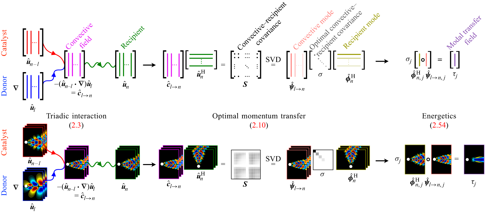
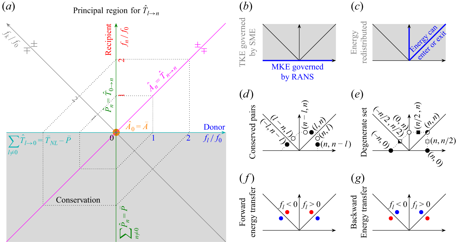


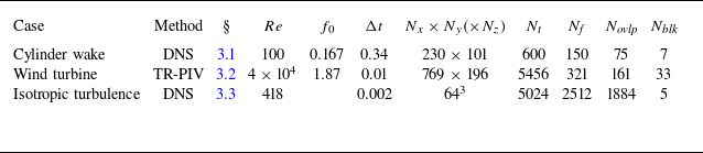

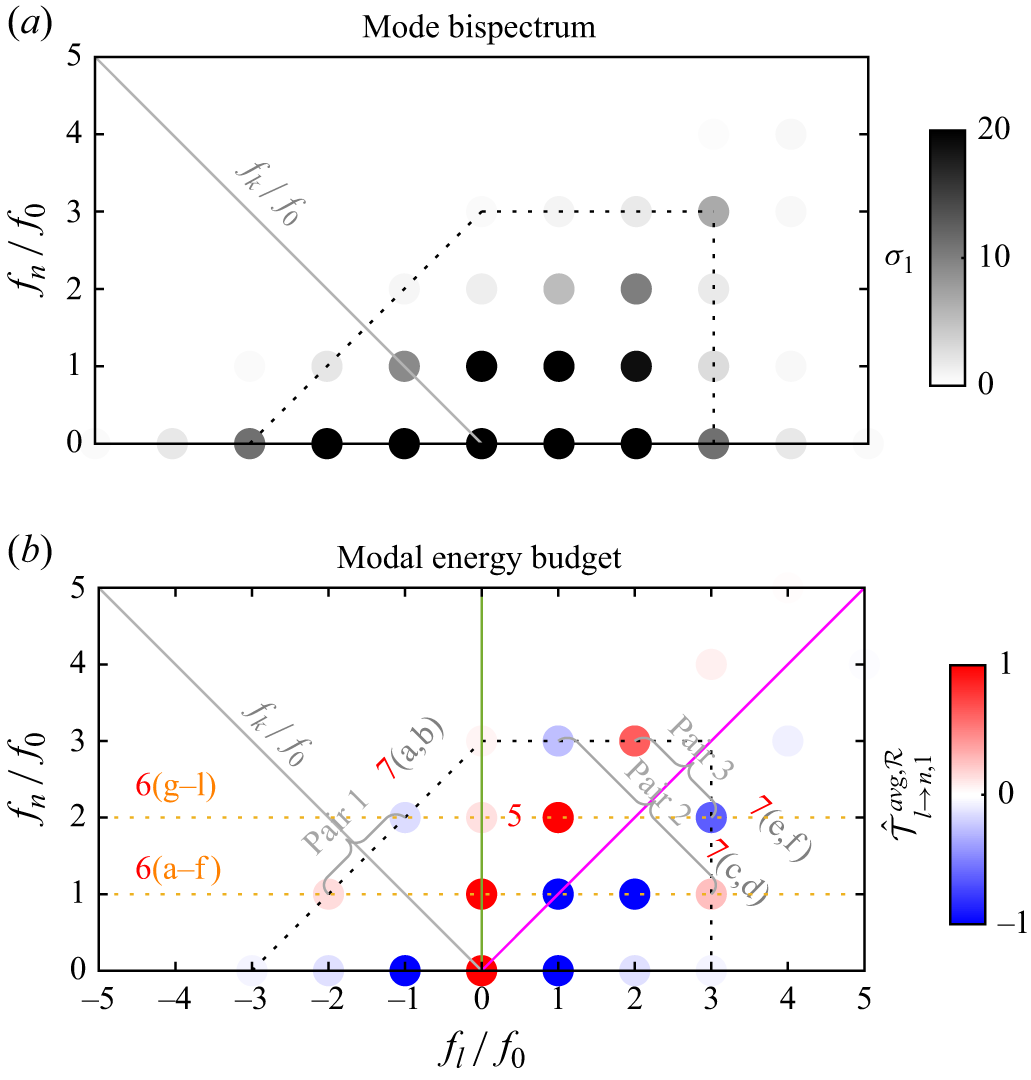


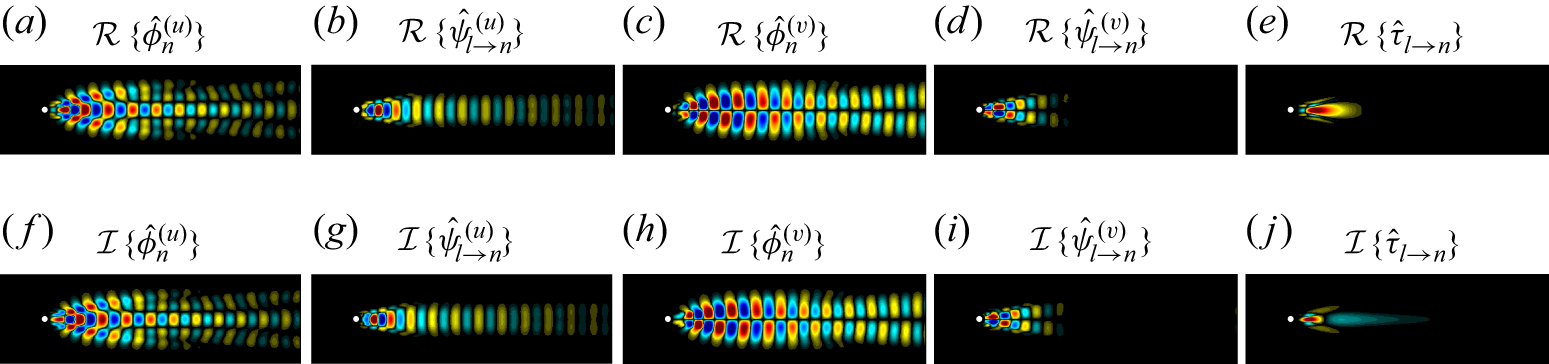


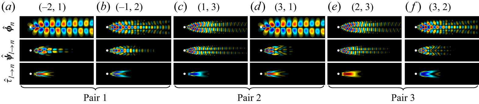
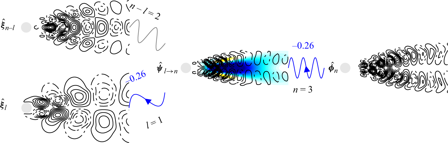


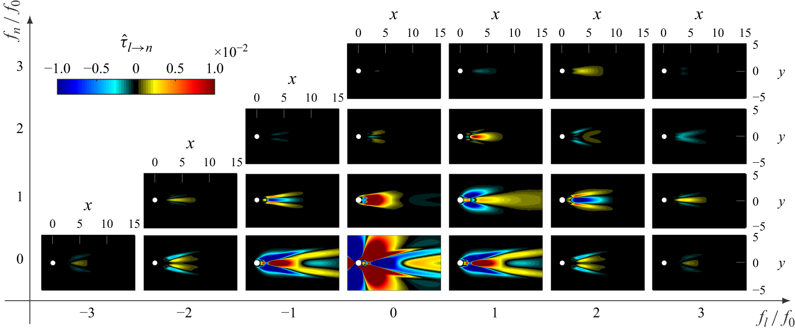
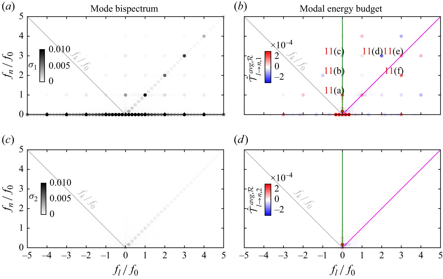


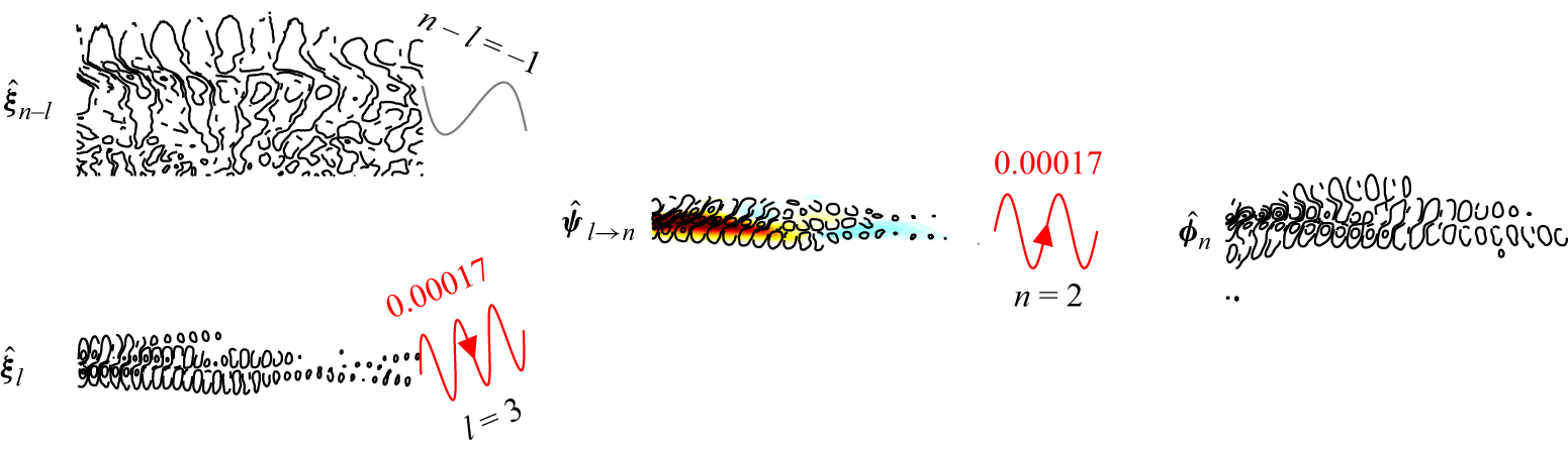


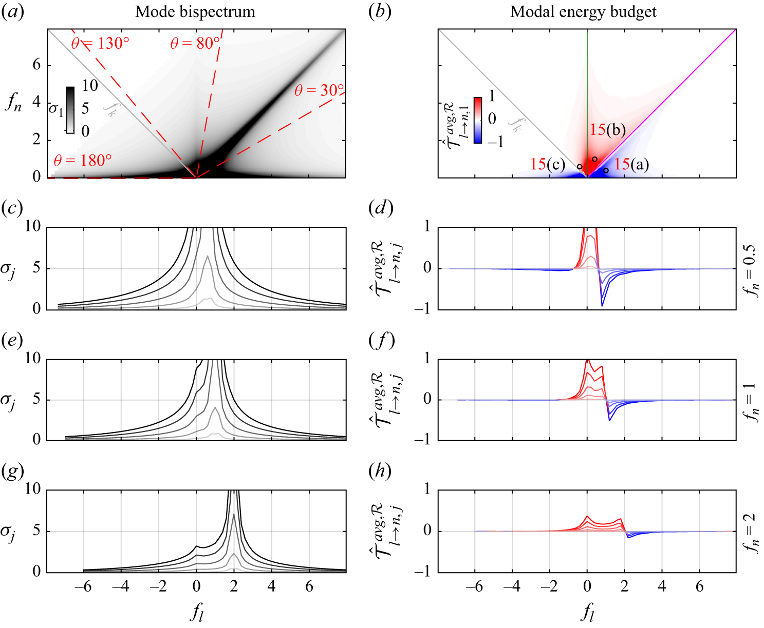


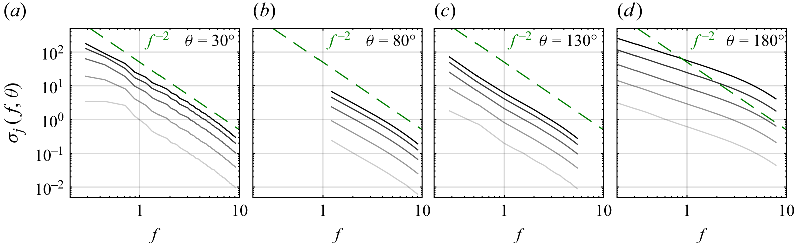


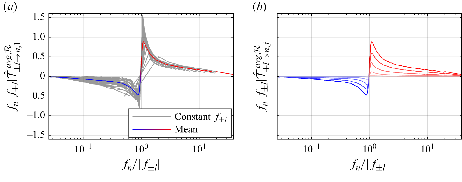


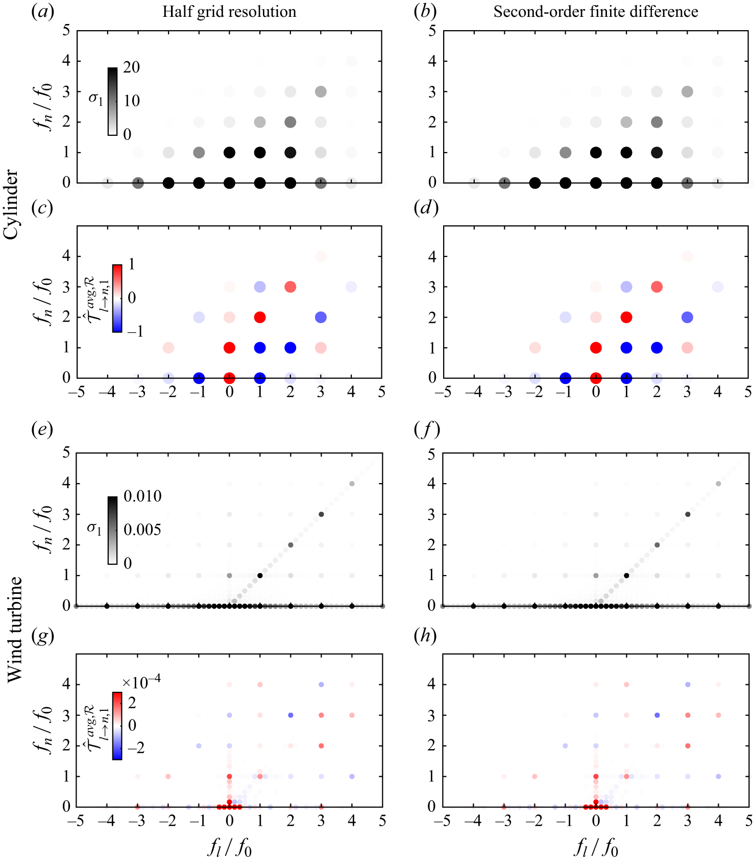


 Open access

