





1. Introduction
The transition from laminar to turbulent flow in boundary layers (BLs) is a key phenomenon in many technical applications, particularly in aerospace engineering. Turbulent BLs exhibit a significantly increased viscous drag and heat flux (Malmuth et al. Reference Malmuth, Fedorov, Shalaev, Cole, Hites, Williams and Khokhlov1998; Fedorov et al. Reference Fedorov, Malmuth, Rasheed and Hornung2001). The latter becomes especially crucial in hypersonic flight, where the higher thermal load demands more robust thermal protection systems – at the expense of overall vehicle performance (Whitehead Reference Whitehead1989). Therefore, understanding and controlling the BL transition process is essential for improving system efficiency and performance. In low-disturbance environments – such as high-altitude flight with smooth surfaces – one key mechanism responsible for BL transition is the amplification of unstable modes (Malik, Zang & Bushnell Reference Malik, Zang and Bushnell1990; Morkovin Reference Morkovin1994). These modes are excited through receptivity processes, in which small environmental disturbances enter the BL and interact with the inherent instabilities (Mack Reference Mack1984; Fedorov Reference Fedorov2015). As a result, the unstable modes begin to grow, initially following the predictions of linear stability theory (LST) before nonlinear effects prevail, leading to the onset of turbulence (Mack Reference Mack1969; Morkovin Reference Morkovin1994; Fedorov Reference Fedorov2015). Linear stability analysis therefore plays a central role for studying the initial phase of BL transition.
Pioneering work on linear boundary layer stability was conducted by Lees & Lin (Reference Lees and Lin1946), who formulated an inviscid stability theory for compressible flows using asymptotic analysis. A foundational contribution in this context was later achieved by the comprehensive numerical investigations of Mack (Reference Mack1969, Reference Mack1984). His results corroborated the earlier predictions of Dunn & Lin (Reference Dunn and Lin1955) and Lees & Reshotko (Reference Lees and Reshotko1962), identifying the emergence of a so-called first mode that becomes unstable from moderate supersonic Mach numbers onward and can be viewed as an extension of the incompressible Tollmien–Schlichting waves to higher flow speeds. While this first mode is primarily viscous at low Mach numbers, its inviscid nature becomes more pronounced with increasing Mach number (Mack Reference Mack1984). In addition, Mack (Reference Mack1963, Reference Mack1964) identified a family of additional instability modes appearing at higher Mach numbers. These higher modes, commonly known as Mack modes, differ in character from the first mode: while the latter is associated with relatively low frequencies and exhibits maximum growth for oblique three-dimensional (3-D) disturbances, the Mack modes are high-frequency acoustic waves of inviscid nature that are most unstable for two-dimensional (2-D) disturbances (Mack Reference Mack1969, Reference Mack1984, Reference Mack1987). They emerge above Mach ${\sim}2.2$
under an adiabatic wall condition (Malmuth et al. Reference Malmuth, Fedorov, Shalaev, Cole, Hites, Williams and Khokhlov1998). The most unstable among these higher modes is the so-called second mode, characterised by the lowest frequency (Mack Reference Mack1984; Reed, Saric & Arnal Reference Reed, Saric and Arnal1996; Malmuth et al. Reference Malmuth, Fedorov, Shalaev, Cole, Hites, Williams and Khokhlov1998), whose existence was already experimentally demonstrated, for example, by Demetriades (Reference Demetriades1974). At Mach numbers above approximately
${\sim}2.2$
under an adiabatic wall condition (Malmuth et al. Reference Malmuth, Fedorov, Shalaev, Cole, Hites, Williams and Khokhlov1998). The most unstable among these higher modes is the so-called second mode, characterised by the lowest frequency (Mack Reference Mack1984; Reed, Saric & Arnal Reference Reed, Saric and Arnal1996; Malmuth et al. Reference Malmuth, Fedorov, Shalaev, Cole, Hites, Williams and Khokhlov1998), whose existence was already experimentally demonstrated, for example, by Demetriades (Reference Demetriades1974). At Mach numbers above approximately $4$
or even lower under wall cooling conditions (Lysenko & Maslov Reference Lysenko and Maslov1984; Malik Reference Malik1989), the second mode becomes the dominant BL instability, surpassing the first mode growth rate.
$4$
or even lower under wall cooling conditions (Lysenko & Maslov Reference Lysenko and Maslov1984; Malik Reference Malik1989), the second mode becomes the dominant BL instability, surpassing the first mode growth rate.
Given the objective of delaying the BL transition, strategies targeting the attenuation of the linear instability modes are of central interest. In this context, the different nature of the first and higher Mack modes proves essential, as it results in the modes responding markedly differently to various control measures. Wall cooling, for instance, has been found to effectively damp the first mode (Lees & Lin Reference Lees and Lin1946), while conversely having an amplifying effect on the second and higher modes (Mack Reference Mack1969, Reference Mack1984). In search of effective damping strategies for the Mack modes, Malmuth et al. (Reference Malmuth, Fedorov, Shalaev, Cole, Hites, Williams and Khokhlov1998) proposed the use of passive porous-wall coatings, assuming that such porous surfaces could absorb the perturbation energy of the high-frequency acoustic modes. Key advantages of porous walls for technical applications are their minimal impact on the mean flow (Fedorov et al. Reference Fedorov, Shiplyuk, Maslov, Burov and Malmuth2003; Tian & Wen Reference Tian and Wen2021). To model the interaction of flow perturbations with acoustic metasurfaces, such as porous linings, an acoustic impedance boundary condition is commonly applied within the framework of LST (Fedorov et al. Reference Fedorov, Malmuth, Rasheed and Hornung2001). In the frequency domain, this condition takes the form $\hat {v}_w=\hat {p}_w/Z$
, relating the amplitudes of the wall-normal velocity perturbations
$\hat {v}_w=\hat {p}_w/Z$
, relating the amplitudes of the wall-normal velocity perturbations $v^{\prime}_w$
and the pressure perturbations
$v^{\prime}_w$
and the pressure perturbations $p^{\prime}_w$
via the complex acoustic surface impedance
$p^{\prime}_w$
via the complex acoustic surface impedance $Z$
(Malmuth et al. Reference Malmuth, Fedorov, Shalaev, Cole, Hites, Williams and Khokhlov1998). The impedance itself is determined by the material and geometrical properties of the wall, the mean flow characteristics (such as Mach number, wall temperature and viscosity), as well as on the wavenumber and frequency of the perturbation (Fedorov et al. Reference Fedorov, Malmuth, Rasheed and Hornung2001).
$Z$
(Malmuth et al. Reference Malmuth, Fedorov, Shalaev, Cole, Hites, Williams and Khokhlov1998). The impedance itself is determined by the material and geometrical properties of the wall, the mean flow characteristics (such as Mach number, wall temperature and viscosity), as well as on the wavenumber and frequency of the perturbation (Fedorov et al. Reference Fedorov, Malmuth, Rasheed and Hornung2001).
Following the foundational work of Malmuth et al. (Reference Malmuth, Fedorov, Shalaev, Cole, Hites, Williams and Khokhlov1998), numerous studies have investigated the influence of acoustic metasurfaces on BL disturbances. It was found that, in contrast to the effect of wall cooling, porous linings induce a slight destabilisation of the first mode, as evidenced both numerically and experimentally (Fedorov et al. Reference Fedorov, Shiplyuk, Maslov, Burov and Malmuth2003; Egorov, Fedorov & Soudakov Reference Egorov, Fedorov and Soudakov2008). By contrast, porous walls can significantly reduce the second-mode instabilities (Malmuth et al. Reference Malmuth, Fedorov, Shalaev, Cole, Hites, Williams and Khokhlov1998; Fedorov et al. Reference Fedorov, Malmuth, Rasheed and Hornung2001, Reference Fedorov, Shiplyuk, Maslov, Burov and Malmuth2003, Reference Fedorov, Kozlov, Shiplyuk, Maslov and Malmuth2006; Egorov et al. Reference Egorov, Fedorov and Soudakov2008; Wagner et al. Reference Wagner, Kuhn, Martinez Schramm and Hannemann2013). To account for the dependence of first-mode destabilisation and higher-mode damping on the specific porous-wall design, several authors, including Brès et al. (Reference Brès, Colonius and Fedorov2010), Tian et al. (Reference Tian, Zhao, Long and Wen2019), Tian et al. (Reference Tian, Liu, Wang, Zhu and Wen2022) and Hammachi et al. (Reference Hammachi, Cardesa, Piot, Montagnac and Deniau2023), have sought to optimise the porous-wall configuration (such as pore depth, density and material composition) to reduce first-mode amplification while maintaining stabilisation of the second and higher modes across a broad frequency range.
In addition to the stabilising and destabilising effects on existing modes, Rienstra (Reference Rienstra2003) further identified the emergence of new instabilities induced by impedance walls. Investigating an inviscid duct flow with constant impedance wall lining, he observed that the so-called surface waves, which are relevant near the wall, can become unstable under specific combinations of Mach number and wall impedance. Rienstra’s theoretical predictions of a hydrodynamic instability over an impedance wall were confirmed experimentally by Aurégan & Leroux (Reference Aurégan and Leroux2008) for a Mach $0.3$
channel flow. Moreover, Brambley (Reference Brambley2013) extended Rienstra’s analysis to a Mach
$0.3$
channel flow. Moreover, Brambley (Reference Brambley2013) extended Rienstra’s analysis to a Mach $0.5$
duct flow by also considering the effects of a thin sheared BL. His studies showed the occurrence of at least one convective instability among up to six possible surface modes when applying an impedance wall modelled either by a Helmholtz resonator or a mass–spring–damper model.
$0.5$
duct flow by also considering the effects of a thin sheared BL. His studies showed the occurrence of at least one convective instability among up to six possible surface modes when applying an impedance wall modelled either by a Helmholtz resonator or a mass–spring–damper model.
In addition to the widely reported stabilising effect of porous walls on the Mack modes, Fedorov et al. (Reference Fedorov, Brès, Inkman and Colonius2011) and Brès et al. (Reference Brès, Inkman, Colonius and Fedorov2013) also identified scenarios in which certain porous-wall configurations can lead to the emergence of a new unstable acoustic mode – highlighting the sensitivity of the effects of porous walls to the specific wall design. Within a temporal stability framework, they investigated the influence of porous walls with rectangular pores on the instabilities in a Mach $6$
BL. They considered the case of strong wall cooling (
$6$
BL. They considered the case of strong wall cooling ( $T_w/T_{\infty } = 1.4$
), for which the first-mode waves are stable. Their study showed that, in addition to the well-known stabilising effect on second-mode instabilities observed for deeper pores, there also exists a particular wall configuration with shallow pores and high porosity that gives rise to a new short-wavelength instability. The newly induced instability, which can exhibit higher growth rates than the conventional second mode, results from a branching behaviour of the dispersion relation and is associated with acoustic resonance within the pores. This phenomenon was also confirmed by means of direct numerical simulation. The non-classical effect observed for porous walls with shallow pores and high porosity aligns with our previous findings for a Mach
$T_w/T_{\infty } = 1.4$
), for which the first-mode waves are stable. Their study showed that, in addition to the well-known stabilising effect on second-mode instabilities observed for deeper pores, there also exists a particular wall configuration with shallow pores and high porosity that gives rise to a new short-wavelength instability. The newly induced instability, which can exhibit higher growth rates than the conventional second mode, results from a branching behaviour of the dispersion relation and is associated with acoustic resonance within the pores. This phenomenon was also confirmed by means of direct numerical simulation. The non-classical effect observed for porous walls with shallow pores and high porosity aligns with our previous findings for a Mach $4.2$
BL over a porous wall with circular pores (De Broeck et al. Reference De Broeck, Görtz, Alter, Hennings de Lara and Oberlack2025). Based on an analytical solution, it was shown that thick porous layers exhibit the well-known behaviour of first-mode destabilisation and second-mode stabilisation, whereas thin porous layers can induce second-mode destabilisation. A marginal second-mode amplification was also observed by Zhao et al. (Reference Zhao, Liu, Wen and Wang2022a
), who designed a piecewise acoustic metasurface aimed at suppressing the first mode across a wide frequency band in a Mach
$4.2$
BL over a porous wall with circular pores (De Broeck et al. Reference De Broeck, Görtz, Alter, Hennings de Lara and Oberlack2025). Based on an analytical solution, it was shown that thick porous layers exhibit the well-known behaviour of first-mode destabilisation and second-mode stabilisation, whereas thin porous layers can induce second-mode destabilisation. A marginal second-mode amplification was also observed by Zhao et al. (Reference Zhao, Liu, Wen and Wang2022a
), who designed a piecewise acoustic metasurface aimed at suppressing the first mode across a wide frequency band in a Mach $4$
BL.
$4$
BL.
All these studies reporting second-mode amplification under specific porous-wall configurations are restricted to particular Mach numbers and typically focus either on individual instability modes or on selected wall parameters. For example, the parameter studies of Fedorov et al. (Reference Fedorov, Brès, Inkman and Colonius2011) and Brès et al. (Reference Brès, Inkman, Colonius and Fedorov2013), which explore variations in porosity and aspect ratio, focus exclusively on 2-D second-mode instabilities. The oblique behaviour and, in particular, the response of the first mode to porous-wall configurations that promote second-mode amplification remain unclear. Additional consideration of the first mode and 3-D disturbances is provided by De Broeck et al. (Reference De Broeck, Görtz, Alter, Hennings de Lara and Oberlack2025), but only for a limited set of discrete porosity values under the assumption of an isothermal BL. To date, a systematic study addressing the diverse effects of porous walls over a broad range of the porous-wall parameters, while accounting for both first- and higher-order modes across a wide Mach number range, is still lacking. This gap motivates the present work. Owing to the large number of governing parameters, however, such a comprehensive parameter study resolving the full wavenumber range over broad porous-wall and Mach number variations becomes computationally highly expensive when based on conventional laminar mean-flow models with an underlying similarity solution. Therefore, in the present work, a simplified exponential mean-flow profile is adopted, which admits an exact solution of the underlying compressible Rayleigh equation. This solution, combined with the evaluation method presented herein, enables the intended comprehensive parameter studies without the occurrence of spurious modes. In view of the model simplifications, the present work is to be understood as a continuation of earlier studies employing simplified boundary-layer profiles, including piecewise linear (Goldstein & Rice Reference Goldstein and Rice1973), exponential (Campos & Serrão Reference Campos and Serrão1998) and hyperbolic tangent profiles (Bower & Liu Reference Bower and Liu1994; Brambley Reference Brambley2013). Given the sensitivity of instability modes to the mean-flow profile, however, the present results should be complemented by subsequent numerical investigations employing more realistic base-flow configurations. The present study provides a foundation for such efforts.
In this work, a regular microstructured porous wall with uniformly spaced cylindrical micro-cavities is considered. The proposed solution framework, however, is not restricted to this specific wall configuration and can be readily extended to alternative impedance models, including those incorporating suction effects, described by the exponential mean-flow profile.
The objective of the present work is to identify distinct porous-wall parameter regimes that lead to different effects on BL stability under insulated-wall conditions. First and foremost, we distinguish the influence of the key wall parameters – porosity and porous layer thickness – on the nature of the destabilised mode, including the wavenumber range and the direction of strongest amplification. Both first- and second-mode disturbances are considered. This enables us to delineate porous-wall parameter configurations that lead to different types of destabilisation. Second, we investigate these phenomena across a wide range of Mach numbers, revealing the occurrence of inviscid instabilities induced by porous walls even in subsonic boundary layers. Third, we examine the question of how porous walls promote the occurrence of supersonic instabilities, given that such instabilities propagating supersonically relative to the free stream are known to play a decisive role in sound radiation (Tam & Hu Reference Tam and Hu1989).
As mentioned, the governing equation in the present work is the compressible Rayleigh equation (CRE), a second-order ordinary differential equation (ODE) describing the amplitude of inviscid normal-mode pressure fluctuations in shear flows. Together with problem-specific boundary conditions (BCs), the CRE gives rise to an eigenvalue problem. To solve this eigenvalue problem, various solution techniques have been employed by different authors for specific shear flow profiles. For the CRE with a BL profile, numerical solutions by means of shooting method are extensively discussed by Mack (Reference Mack1984) and Malik (Reference Malik1989). Alternatively, Türkyilmazoglu (Reference Türkyilmazoglu2006) employed a combination of collocation and shooting methods to identify absolute and convective instabilities in a compressible boundary layer over a rotating disk. Compared with these numerical approaches, analytical solutions to the CRE are rare due to the singularities in its coefficient functions and the requirement of an explicit formulation of the mean shear profile. For the simplest case of a constant velocity profile, the CRE is solved in terms of complex exponential functions, which can describe both exponential growth and wave-like behaviour (Lees & Lin Reference Lees and Lin1946). For a linear velocity profile as a simplified model of a duct boundary-layer flow, Goldstein & Rice (Reference Goldstein and Rice1973) were the first to derive an analytical solution of the isothermal form of the CRE, known as the Pridmore–Brown equation (PBE), in terms of combined parabolic cylinder functions. This was achieved by reducing the PBE to Weber’s equation via suitable transformations of the dependent and independent variables. Assuming a hyperbolic tangent profile, Bower & Liu (Reference Bower and Liu1994) employed the Wentzel–Kramers–Brillouin (WKB) method to obtain a solution for the CRE in terms of Airy functions. Their results for two-dimensional neutral perturbations showed good qualitative agreement with the numerical results of Mack (Reference Mack1984). Zhang & Oberlack (Reference Zhang and Oberlack2021) solved the PBE for an exponential BL profile in terms of confluent Heun functions. This solution allowed the BL stability problem to be reduced to an algebraic dispersion relation. Building on this formulation, De Broeck et al. (Reference De Broeck, Görtz, Alter, Hennings de Lara and Oberlack2025) retained the same isothermal exponential BL model and extended the Heun-based dispersion relation introduced by Zhang & Oberlack for the rigid-wall configuration to account for impedance walls. In the present work, we broaden the analysis to include non-isothermal effects. For the non-isothermal BL, we again adopt an exponential velocity profile as an intentionally simplified mean-flow model, chosen to facilitate analytical progress rather than to represent the most accurate compressible BL. This analytical description of the mean velocity allows us to derive a closed-form solution of the CRE in terms of general Heun functions, which in turn yields an algebraic eigenvalue equation that forms the basis of the linear stability analysis.
The paper is structured as follows. Section 2 outlines the underlying model equations, the CRE and the associated boundary conditions used to describe the inviscid linear BL stability. The velocity and temperature BL profiles along with the porous-wall model considered in this work are introduced in § 3. Using the analytical solution of the CRE derived for the chosen exponential profile, we can transform the BL problem into an algebraic eigenvalue equation describing the inviscid modal disturbances within the BL. The numerical algorithm for solving the eigenvalue equation is presented in § 4. Applying this algorithm, we compute the complex eigenvalues $\omega$
for the temporal stability case across a broad wavenumber spectrum. We first perform the eigenvalue analysis under systematic variation of the porous-wall parameters in § 5, focusing on their influence on the key characteristics of the dominant instability, including growth rate, phase speed and propagation direction. Subsequently, in § 6, the analysis is extended to a wide Mach number range.
$\omega$
for the temporal stability case across a broad wavenumber spectrum. We first perform the eigenvalue analysis under systematic variation of the porous-wall parameters in § 5, focusing on their influence on the key characteristics of the dominant instability, including growth rate, phase speed and propagation direction. Subsequently, in § 6, the analysis is extended to a wide Mach number range.
2. Basic model equations
We start by formulating the underlying model equations that describe the linear stability of the compressible BL flow. Given the increasingly inviscid character of the dominant instability mechanisms with rising Mach number, inviscid stability theory already provides key physical insights (Mack Reference Mack1969, Reference Mack1984). The stability problem is therefore formulated on the compressible linearised Euler equations, from which the CRE for plane shear-flow disturbances can be derived (§ 2.1). The CRE, together with specific boundary conditions for boundary layer stability over porous wall, provides the eigenvalue problem for our stability analysis (§ 2.2).
2.1. Compressible Rayleigh equation
We start from the compressible linearised Euler equations. As the focus lies on the inviscid acoustic modes in BLs of high Reynolds numbers, the effects of heat conduction on the disturbances are neglected (Rienstra & Hirschberg Reference Rienstra and Hirschberg2001; Delfs Reference Delfs2016). Under these assumptions, which are particularly valid for high frequency ranges (Aurégan et al. Reference Aurégan, Starobinski and Pagneux2001; Brambley Reference Brambley2011), the linearised Euler equations (LEEs) can be written in the form (Criminale, Jackson & Joslin Reference Criminale, Jackson and Joslin2018; Görtz Reference Görtz2025)
 \begin{align} \frac {{\rm D}_0 \rho ^{\prime }}{{\rm D} t}+\rho _0 \boldsymbol{\nabla } \boldsymbol \cdot \boldsymbol{v}^{\prime }+\boldsymbol{v}^{\prime } \boldsymbol \cdot \boldsymbol{\nabla }\rho _0+\rho ^{\prime } \boldsymbol{\nabla } \boldsymbol \cdot \boldsymbol{v}_0 &=0 , \end{align}
 \begin{align} \rho _0 \frac {{\rm D}_0 \boldsymbol{v}^{\prime }}{{\rm D} t}+\boldsymbol{\nabla }p^{\prime }+\rho _0 \boldsymbol{v}^{\prime } \boldsymbol \cdot \boldsymbol{\nabla }\boldsymbol{v}_0+\rho ^{\prime } \boldsymbol{v}_0 \boldsymbol \cdot \boldsymbol{\nabla } \boldsymbol{v}_0 &=0 , \end{align}
 \begin{align} \frac {1}{c_0^{2}}\left (\frac {{\rm D}_0 p^{\prime }}{{\rm D} t}+\boldsymbol{v}^{\prime } \boldsymbol \cdot \boldsymbol{\nabla }p_0\right )+\rho _0 \boldsymbol{\nabla } \boldsymbol \cdot \boldsymbol{v}^{\prime }+\left (\rho _0 \frac {c^{\prime 2}}{c_0^{2}}+\rho ^{\prime }\right ) \boldsymbol{\nabla } \boldsymbol \cdot \boldsymbol{v}_0 &=0 , \end{align}
representing a set of partial differential equations (PDEs) for the small unsteady perturbations, denoted by prime, linearised around the mean flow state, indexed by 0. Here, $p$
denotes the pressure,
$p$
denotes the pressure, $\rho$
the density and
$\rho$
the density and $\boldsymbol{v}=(u,v,w)^T$
the velocity vector, while
$\boldsymbol{v}=(u,v,w)^T$
the velocity vector, while $c$
is the speed of sound and
$c$
is the speed of sound and $ {{\rm D}_0}/{{\rm D} t}:=({\partial }/{\partial t})+ (\boldsymbol{v}_0 \boldsymbol \cdot \boldsymbol{\nabla })$
the material derivative with respect to the mean flow.
$ {{\rm D}_0}/{{\rm D} t}:=({\partial }/{\partial t})+ (\boldsymbol{v}_0 \boldsymbol \cdot \boldsymbol{\nabla })$
the material derivative with respect to the mean flow.
In view of the BL problem, the base flow is assumed as a plane shear layer $\boldsymbol{v}_0=U_0(y) \cdot \boldsymbol{e}_x$
, depending only on the wall-normal direction
$\boldsymbol{v}_0=U_0(y) \cdot \boldsymbol{e}_x$
, depending only on the wall-normal direction $y$
, with
$y$
, with $y=0$
denoting the wall surface. Furthermore, the base flow is considered to be non-isentropic, non-isothermal with a mean temperature gradient
$y=0$
denoting the wall surface. Furthermore, the base flow is considered to be non-isentropic, non-isothermal with a mean temperature gradient $T_0(y)$
normal to the wall and constant pressure
$T_0(y)$
normal to the wall and constant pressure $p_0$
. For ideal gas, the equation of state thus gives
$p_0$
. For ideal gas, the equation of state thus gives
 \begin{equation} \rho _0(y)=\frac {p_0}{RT_0(y)} \end{equation}
and the speed of sound can be expressed by
 \begin{equation} c_0^{2}(y)=\gamma R T_0(y), \end{equation}
with $R$
as the ideal gas constant and
$R$
as the ideal gas constant and $\gamma$
the isentropic exponent.
$\gamma$
the isentropic exponent.
The LEEs resulting for these BL assumptions are non-dimensionalised by using the BL thickness $\delta$
, the free stream velocity
$\delta$
, the free stream velocity $U_{\infty }$
and the mean pressure
$U_{\infty }$
and the mean pressure $p_0$
scaled with
$p_0$
scaled with $\gamma$
, giving as reference scales for the dynamic quantities
$\gamma$
, giving as reference scales for the dynamic quantities
 \begin{equation} p_{\textit{ref}}=p_0 \gamma ,\qquad \rho _{\textit{ref}}=\frac {p_0\gamma M^2}{U_\infty ^2},\qquad T_{\textit{ref}}=T_\infty =\frac {U_\infty ^2}{\gamma R M^2}. \end{equation}
As a result, in the non-dimensionalised LEE system, the Mach number $M=U_{\infty }/c_{\infty }$
arises as dimensionless parameter, with
$M=U_{\infty }/c_{\infty }$
arises as dimensionless parameter, with $c_{\infty }$
referring to the speed of sound in the far field. Note that from now on all quantities are non-dimensionalised.
$c_{\infty }$
referring to the speed of sound in the far field. Note that from now on all quantities are non-dimensionalised.
Using the homogeneity of the equations with respect to $x$
,
$x$
, $z$
and
$z$
and $t$
, the perturbations can be expressed by a normal mode approach according to
$t$
, the perturbations can be expressed by a normal mode approach according to
 \begin{align} q^\prime (x,y,z,t)=\hat {q}(y)e^{i(\alpha x+\beta z-\omega t)}, \quad \text{with} \; q^\prime \in \left \{u^\prime ,v^\prime , w^\prime ,p^\prime ,\rho ^\prime , T^\prime \right \} , \end{align}
where $\hat {q}(y)$
is the complex amplitude of the dimensionless perturbations. It is a function only of the wall-normal coordinate
$\hat {q}(y)$
is the complex amplitude of the dimensionless perturbations. It is a function only of the wall-normal coordinate $y$
. In the context of temporal stability analysis as intended in this work,
$y$
. In the context of temporal stability analysis as intended in this work, $\omega$
is assumed to be complex, i.e.
$\omega$
is assumed to be complex, i.e. $\omega \in \mathbb{C}$
, with its imaginary part
$\omega \in \mathbb{C}$
, with its imaginary part $\omega _i$
representing the temporal growth rate. Due to the choice of signs in (2.5),
$\omega _i$
representing the temporal growth rate. Due to the choice of signs in (2.5), $\omega _i\gt 0$
implies unstable exponential growth. The real part
$\omega _i\gt 0$
implies unstable exponential growth. The real part $\omega _r$
corresponds to the temporal frequency. Here,
$\omega _r$
corresponds to the temporal frequency. Here, $\alpha , \beta \in \mathbb{R}$
describe the dimensionless streamwise and spanwise wavenumbers. Inserting (2.5) into the non-dimensionalised LEEs transforms the PDE system into a system of ODEs for the perturbation amplitudes. Decoupling this ODE system leads to a single second-order ODE for the pressure perturbation amplitude
$\alpha , \beta \in \mathbb{R}$
describe the dimensionless streamwise and spanwise wavenumbers. Inserting (2.5) into the non-dimensionalised LEEs transforms the PDE system into a system of ODEs for the perturbation amplitudes. Decoupling this ODE system leads to a single second-order ODE for the pressure perturbation amplitude $\hat {p}(y)$
can be derived, the compressible Rayleigh equation (Criminale et al. Reference Criminale, Jackson and Joslin2018),
$\hat {p}(y)$
can be derived, the compressible Rayleigh equation (Criminale et al. Reference Criminale, Jackson and Joslin2018),
 \begin{equation} \frac {{\rm d}^2 \hat p }{{\rm d}y^2}+\left [\frac {2\alpha U_0^{\prime}(y)}{\omega -\alpha U_0(y)}+\frac {T_0^{\prime}(y)}{T_0(y)}\right ]\frac {{\rm d} \hat p }{{\rm d}y}+\left [\frac {M^2\left (\omega -\alpha U_0(y)\right )^2}{T_0(y)}-\alpha ^2-\beta ^2\right ]\hat p(y)=0 , \end{equation}
where from now on, the prime denotes the derivative with respect to $y$
. From
$y$
. From $\hat {p} (y)$
, the perturbation amplitudes of velocity, density and temperature follow from the decoupled ODEs, reading
$\hat {p} (y)$
, the perturbation amplitudes of velocity, density and temperature follow from the decoupled ODEs, reading
 \begin{align} \hat {u}&=-\frac {U_0^{\prime}\,T_0}{M^{2}(\omega -U_0\alpha )^{2}}\,\frac {{\rm d}\hat p }{{\rm d}y}+\frac {\alpha T_0}{M^{2}(\omega -U_0\alpha )}\hat {p}, \end{align}
 \begin{align} \hat {v}&=-\frac {i T_0}{M^{2}(\omega -U_0\alpha )}\,\frac {{\rm d} \hat p }{{\rm d}y}, \end{align}
 \begin{align} \hat {w}&=\frac {\beta \, T_0}{M^{2}(\omega -U_0\alpha )}\,\hat p(y), \end{align}
 \begin{align} \hat {\rho }&=\frac {1}{i(\omega -U_0\alpha )}\left [\frac {1}{T_0}\left (i\alpha \,\hat u + \frac {{\rm d}\hat v}{{\rm d}y} \right )+\hat v\frac {{\rm d}}{{\rm d}y}\left (\frac {1}{T_0}\right )\right ]\! , \end{align}
 \begin{align} \hat {T}&=\gamma \, T_0 \hat p -T_0^2\hat \rho . \end{align}
2.2. Boundary conditions
A central part of the physics to be investigated subsequently lies in the problem-specific BCs for $\hat {p}$
. Regarding the behaviour in the far field (
$\hat {p}$
. Regarding the behaviour in the far field ( $y\to \infty$
), we require bounded perturbation amplitudes (Mack Reference Mack1984), as we focus on the stability behaviour of the BL itself without energy transport from the free stream into the BL. It should be noted that other authors, such as Brazier-Smith & Scott (Reference Brazier-Smith and Scott1984), Huerre & Monkewitz (Reference Huerre and Monkewitz1985), Crighton (Reference Crighton1989), Riedinger et al. (Reference Riedinger, Le Dizès and Meunier2010) and Brambley & Gabard (Reference Brambley and Gabard2014), suggest a different far-field condition grounded on causality arguments, which allows unbound behaviour in the far field for neutrally stable or damped modes (
$y\to \infty$
), we require bounded perturbation amplitudes (Mack Reference Mack1984), as we focus on the stability behaviour of the BL itself without energy transport from the free stream into the BL. It should be noted that other authors, such as Brazier-Smith & Scott (Reference Brazier-Smith and Scott1984), Huerre & Monkewitz (Reference Huerre and Monkewitz1985), Crighton (Reference Crighton1989), Riedinger et al. (Reference Riedinger, Le Dizès and Meunier2010) and Brambley & Gabard (Reference Brambley and Gabard2014), suggest a different far-field condition grounded on causality arguments, which allows unbound behaviour in the far field for neutrally stable or damped modes ( $\omega _i\lt 0$
). However, with respect to temporally unstable perturbations (
$\omega _i\lt 0$
). However, with respect to temporally unstable perturbations ( $\omega _i\gt 0$
), there is agreement on the boundedness of the perturbations at infinity. In the following study, we will restrict our analysis to unstable disturbances due to their relevance for the BL transition.
$\omega _i\gt 0$
), there is agreement on the boundedness of the perturbations at infinity. In the following study, we will restrict our analysis to unstable disturbances due to their relevance for the BL transition.
A stricter requirement, also commonly used in stability theory, is the constraint of vanishing amplitudes in the far field, which gives us the boundary condition
 \begin{equation} \lim _{y\to \infty }\hat {p }(y)=0 . \end{equation}
It should be mentioned that for our model equations, boundedness of the far-field amplitudes can only be realised by vanishing amplitudes in the case of $\omega _i\neq 0$
, as we will see later in § 3.2. This implies that the same eigenvalues of the stability problem would also arise under the less strict far-field condition requiring bounded perturbations.
$\omega _i\neq 0$
, as we will see later in § 3.2. This implies that the same eigenvalues of the stability problem would also arise under the less strict far-field condition requiring bounded perturbations.
To describe the effect of acoustic metasurfaces like a porous wall on the BL disturbances, we introduce the complex acoustic wall impedance $Z$
, which links the pressure perturbation to the wall-normal velocity perturbation at the wall (Hubbard Reference Hubbard1991; Malmuth et al. Reference Malmuth, Fedorov, Shalaev, Cole, Hites, Williams and Khokhlov1998), which can be expressed in the frequency–wavenumber domain as
$Z$
, which links the pressure perturbation to the wall-normal velocity perturbation at the wall (Hubbard Reference Hubbard1991; Malmuth et al. Reference Malmuth, Fedorov, Shalaev, Cole, Hites, Williams and Khokhlov1998), which can be expressed in the frequency–wavenumber domain as
 \begin{equation} \hat {p}(y; \alpha , \beta , \omega )=-Z\,\hat {v}(y; \alpha , \beta , \omega ) \quad \text{at }\, y=0 . \end{equation}
The latter form results from the impedance wall condition given in the Laplace domain for vanishing mean wall flow, as found, for example, in Malmuth et al. (Reference Malmuth, Fedorov, Shalaev, Cole, Hites, Williams and Khokhlov1998) and Rienstra (Reference Rienstra2006). This is Fourier transformed under the assumptions of a straight wall with homogeneous impedance $Z$
, yielding (2.9). The wall impedance
$Z$
, yielding (2.9). The wall impedance $Z$
itself is a function of the disturbance frequency and wavenumber, as well as on the wall properties and characteristics of the mean flow, like the Mach number (Malmuth et al. Reference Malmuth, Fedorov, Shalaev, Cole, Hites, Williams and Khokhlov1998; Zhao et al. Reference Zhao, Wen, Zhou, Tu and Lei2022b
). From (2.9), we derive a second BC for the pressure amplitude
$Z$
itself is a function of the disturbance frequency and wavenumber, as well as on the wall properties and characteristics of the mean flow, like the Mach number (Malmuth et al. Reference Malmuth, Fedorov, Shalaev, Cole, Hites, Williams and Khokhlov1998; Zhao et al. Reference Zhao, Wen, Zhou, Tu and Lei2022b
). From (2.9), we derive a second BC for the pressure amplitude $\hat {p}$
by expressing
$\hat {p}$
by expressing $\hat {v}$
by
$\hat {v}$
by $\hat {p}$
via (2.7b
), which yields
$\hat {p}$
via (2.7b
), which yields
 \begin{equation} \left .\frac {{\rm d}\hat {p}}{{\rm d}y}\right |_{y=0}=-i\omega \,Y\frac {M^2}{T_w}\hat {p}(0), \, \end{equation}
where $Y=Z^{-1}$
is the acoustic admittance. Note that the limit
$Y=Z^{-1}$
is the acoustic admittance. Note that the limit $Z\to \infty$
or
$Z\to \infty$
or $Y=0$
corresponds to the case of a rigid wall (Campos & Serrão Reference Campos and Serrão1998).
$Y=0$
corresponds to the case of a rigid wall (Campos & Serrão Reference Campos and Serrão1998).
Both BCs (2.8) and (2.10) together with the CRE (2.6) form the boundary value problem for the acoustic disturbances in the considered BL flow, providing an eigenvalue problem for the normal mode parameters $(\alpha , \beta , \omega )$
, ensuring compatibility of the CRE solutions with the BCs.
$(\alpha , \beta , \omega )$
, ensuring compatibility of the CRE solutions with the BCs.
3. Analytical solution and eigenvalue equation for the specific model
For the velocity and the temperature profiles $U_0(y)$
and
$U_0(y)$
and $T_0(y)$
, discussed in § 3.1, we will derive an analytical solution of the CRE. This solution, together with the BCs, reduces the differential eigenvalue problem to an algebraic equation (§ 3.2). For the wall admittance
$T_0(y)$
, discussed in § 3.1, we will derive an analytical solution of the CRE. This solution, together with the BCs, reduces the differential eigenvalue problem to an algebraic equation (§ 3.2). For the wall admittance $Y$
in the eigenvalue equation, we apply a porous-wall model (§ 3.3).
$Y$
in the eigenvalue equation, we apply a porous-wall model (§ 3.3).
3.1. Velocity and temperature profile
To model the mean velocity in the BL flow, we adopt an exponential shear profile
 \begin{align} U_0(y)=1-e^{-y} , \end{align}
whereby (3.1) is the dimensionless form scaled with $U_{\infty }$
and
$U_{\infty }$
and $\delta$
. The advantage of describing the velocity profile explicitly as an exponential function is that it allows us to derive an analytical solution for the underlying CRE, which in turn enables the BL stability problem to be recast as an algebraic eigenvalue equation. Building on this equation, together with an algebraic solution algorithm, we are able to carry out comprehensive eigenvalue analyses over a wide parameter range without the occurrence of spurious modes. It should be noted, however, that the exponential profile (3.1) does not correspond to a solution of the compressible BL equations, but rather represents a simplifying model assumption. Due to this simplification, the results obtained in this work may deviate quantitatively in their absolute values from those obtained for a more realistic BL profile. Nevertheless, the observed qualitative behaviour is expected to be retained even under other, more common profiles, as explained at the beginning of 5.
$\delta$
. The advantage of describing the velocity profile explicitly as an exponential function is that it allows us to derive an analytical solution for the underlying CRE, which in turn enables the BL stability problem to be recast as an algebraic eigenvalue equation. Building on this equation, together with an algebraic solution algorithm, we are able to carry out comprehensive eigenvalue analyses over a wide parameter range without the occurrence of spurious modes. It should be noted, however, that the exponential profile (3.1) does not correspond to a solution of the compressible BL equations, but rather represents a simplifying model assumption. Due to this simplification, the results obtained in this work may deviate quantitatively in their absolute values from those obtained for a more realistic BL profile. Nevertheless, the observed qualitative behaviour is expected to be retained even under other, more common profiles, as explained at the beginning of 5.
A brief remark is additionally required concerning the definition of the boundary-layer thickness $\delta$
: from (3.1), it follows that at the height of
$\delta$
: from (3.1), it follows that at the height of $y=1$
, corresponding to a wall distance of
$y=1$
, corresponding to a wall distance of $\delta$
, we have
$\delta$
, we have $U_0(1)=1-\mathrm{exp}(-1)\approx 0.63$
, i.e.
$U_0(1)=1-\mathrm{exp}(-1)\approx 0.63$
, i.e. $63\,\%$
of the free stream velocity
$63\,\%$
of the free stream velocity $U_\infty$
. Thus, the BL thickness
$U_\infty$
. Thus, the BL thickness $\delta$
in this work does not represent the
$\delta$
in this work does not represent the $\delta _{99}$
thickness.
$\delta _{99}$
thickness.
Regarding the temperature profile $T_0(y)$
, we formulate a quadratic relationship to the velocity
$T_0(y)$
, we formulate a quadratic relationship to the velocity $U_0(y)$
. This goes back to the temperature relation derived by Crocco’s method (Crocco Reference Crocco1948; Van Driest Reference Van Driest1952a
,
Reference Van Driestb
) for a flat plate BL flow without pressure gradient, which can be written, in case of Prandtl number
$U_0(y)$
. This goes back to the temperature relation derived by Crocco’s method (Crocco Reference Crocco1948; Van Driest Reference Van Driest1952a
,
Reference Van Driestb
) for a flat plate BL flow without pressure gradient, which can be written, in case of Prandtl number ${\textit{Pr}}=1$
, as
${\textit{Pr}}=1$
, as
 \begin{equation} T_0(y)=T_w+(T_{\textit{a}w}-T_w)U_0(y)+(1-T_{\textit{a}w})U_0(y)^2 . \end{equation}
The latter form is also known as the Crocco temperature–velocity relation. Here, $T_w$
describes the wall temperature and
$T_w$
describes the wall temperature and $T_{\textit{a}w}$
the adiabatic wall temperature, which refers to the wall temperature in the case of an insulated wall. With regards to the Crocco relation (3.2), we note that its derivation assumes that the mean velocity profile satisfies the compressible Blasius boundary layer equations (Van Driest Reference Van Driest1952b
), which is not the case for the exponential profile adopted in the present study. Nevertheless, the temperature profile obtained from (3.2) when the exponential velocity profile is inserted reproduces the principal qualitative characteristics of the Crocco temperature profile associated with the Blasius solution sufficiently well. We therefore regard the exponential velocity profile, together with the resulting temperature profile, as an adequate model to represent the key physical features of the BL. This choice should be understood in view of the purpose of the present work to formulate a model problem that allows the fundamental effects to be investigated in a qualitative manner. In the non-dimensional relation (3.2), both
$T_{\textit{a}w}$
the adiabatic wall temperature, which refers to the wall temperature in the case of an insulated wall. With regards to the Crocco relation (3.2), we note that its derivation assumes that the mean velocity profile satisfies the compressible Blasius boundary layer equations (Van Driest Reference Van Driest1952b
), which is not the case for the exponential profile adopted in the present study. Nevertheless, the temperature profile obtained from (3.2) when the exponential velocity profile is inserted reproduces the principal qualitative characteristics of the Crocco temperature profile associated with the Blasius solution sufficiently well. We therefore regard the exponential velocity profile, together with the resulting temperature profile, as an adequate model to represent the key physical features of the BL. This choice should be understood in view of the purpose of the present work to formulate a model problem that allows the fundamental effects to be investigated in a qualitative manner. In the non-dimensional relation (3.2), both $T_w$
and
$T_w$
and $T_{\textit{a}w}$
are dimensionless parameters, scaled by the far-field temperature
$T_{\textit{a}w}$
are dimensionless parameters, scaled by the far-field temperature $T_{\infty }$
. For
$T_{\infty }$
. For ${\textit{Pr}}=1$
, the adiabatic wall temperature is determined by
${\textit{Pr}}=1$
, the adiabatic wall temperature is determined by
 \begin{equation} T_{\textit{a}w}=1+\frac {\gamma -1}{2}M^2 , \end{equation}
where $\gamma$
is the specific heat capacity ratio, with
$\gamma$
is the specific heat capacity ratio, with $\gamma \approx 1.4$
for air.
$\gamma \approx 1.4$
for air.
In the context of this work, we propose a modified quadratic temperature–velocity relation
 \begin{equation} T_0(y)=T_w\,\left (1-\tilde T\,U_0(y)\right )^2 \quad \text{with}\quad \tilde {T}=1-\sqrt {\frac {1}{T_w}} , \end{equation}
which allows the derivation of an analytical solution of the CRE, as discussed in the next section.
Comparison of the simplified temperature relation (3.4) with the full Crocco relation (3.2) shows that the degree of qualitative agreement depends on the wall temperature $T_w$
relative to
$T_w$
relative to $T_{\textit{a}w}$
. This can be seen in figure 1, which compares the simplified temperature relation (solid line) with the full Crocco relation (dashed line) plotted over the wall-normal coordinate
$T_{\textit{a}w}$
. This can be seen in figure 1, which compares the simplified temperature relation (solid line) with the full Crocco relation (dashed line) plotted over the wall-normal coordinate $y$
, both being evaluated using the exponential velocity profile. The two temperature profiles are shown for different wall temperature–Mach number configurations: (a) the insulated-wall case,
$y$
, both being evaluated using the exponential velocity profile. The two temperature profiles are shown for different wall temperature–Mach number configurations: (a) the insulated-wall case, $T_w = T_{\textit{a}w}$
, assumed throughout this study, shown for three Mach numbers
$T_w = T_{\textit{a}w}$
, assumed throughout this study, shown for three Mach numbers $M=0.8, 2.5, 3$
; and, for comparison, (b) a cooled-wall case with
$M=0.8, 2.5, 3$
; and, for comparison, (b) a cooled-wall case with $T_w = 0.5\,T_{\textit{a}w}$
at
$T_w = 0.5\,T_{\textit{a}w}$
at $M=3$
. The figure reveals that, for the adiabatic wall cases (
$M=3$
. The figure reveals that, for the adiabatic wall cases ( $T_w = T_{\textit{a}w}$
), both temperature profiles agree sufficiently well for the purposes of the model problem examined in the present work. This, however, does not hold for the cooled-wall case, where a local maximum appears in the full Crocco profile that is not reproduced by the simplified profile. It can therefore be concluded that the simplified temperature relation captures the qualitative shape of the full Crocco relation sufficiently well only for wall-temperature ratios
$T_w = T_{\textit{a}w}$
), both temperature profiles agree sufficiently well for the purposes of the model problem examined in the present work. This, however, does not hold for the cooled-wall case, where a local maximum appears in the full Crocco profile that is not reproduced by the simplified profile. It can therefore be concluded that the simplified temperature relation captures the qualitative shape of the full Crocco relation sufficiently well only for wall-temperature ratios $T_w/T_{\textit{a}w}$
for which the full Crocco profile does not exhibit a maximum within the BL. From this requirement, limits on permissible wall temperatures can be derived. For the Crocco relation (3.2), the maximum occurs at
$T_w/T_{\textit{a}w}$
for which the full Crocco profile does not exhibit a maximum within the BL. From this requirement, limits on permissible wall temperatures can be derived. For the Crocco relation (3.2), the maximum occurs at
 \begin{equation} U_{0,{\textit{max}}}=\frac {T_{\textit{a}w}-T_w}{2(T_{\textit{a}w}-1)} . \end{equation}
To ensure that this maximum does not occur within the BL region where $U_0\in (0,1)$
applies, we require
$U_0\in (0,1)$
applies, we require $ U_{0,{\textit{max}}} \geqslant 1$
or
$ U_{0,{\textit{max}}} \geqslant 1$
or $ U_{0,{\textit{max}}}\leqslant 0$
, which together with (3.5) results in the wall temperature limits
$ U_{0,{\textit{max}}}\leqslant 0$
, which together with (3.5) results in the wall temperature limits
 \begin{equation} T_w \leqslant 2-T_{\textit{a}w} \quad \! \! \text{for} \; M\lt \sqrt {5} \quad \text{or} \quad T_w \geqslant T_{\textit{a}w} . \end{equation}
The restriction $M\lt \sqrt {5}$
for the lower limit results from the requirement of non-negative temperatures,
$M\lt \sqrt {5}$
for the lower limit results from the requirement of non-negative temperatures, $T_w \gt 0$
, as becomes evident when substituting the relation for
$T_w \gt 0$
, as becomes evident when substituting the relation for $T_{\textit{a}w}$
with
$T_{\textit{a}w}$
with $\gamma =1.4$
into (3.6). Accordingly, (3.6) represent those ranges for
$\gamma =1.4$
into (3.6). Accordingly, (3.6) represent those ranges for $T_w$
for which the Crocco relation (3.2) does not show a local maximum in the BL domain, allowing our simplified relation (3.4) to be used as an approximation.
$T_w$
for which the Crocco relation (3.2) does not show a local maximum in the BL domain, allowing our simplified relation (3.4) to be used as an approximation.
Comparison of the full Crocco temperature relation (3.2) (dashed line) with the modified relation (3.4) (solid line) for adiabatic wall BLs of different Mach numbers and for a cooled-wall BL.

Figure 1. Long description
The line graph compares the full Crocco temperature relation (3.2) with the modified relation (3.4) for adiabatic wall boundary layers of different Mach numbers and for a cooled-wall boundary layer. The x-axis represents the temperature ratio (T), ranging from 1 to 3, while the y-axis represents the distance (y), ranging from 0 to 6. Four data lines are plotted: one for M equals 0.8, T_w equals T_aw; one for M equals 2.5, T_w equals T_aw; one for M equals 3.0, T_w equals T_aw; and one for M equals 3.0, T_w equals 0.5 T_aw. Each line shows how the temperature ratio changes with distance for different Mach numbers and wall temperatures. The dashed lines represent the full Crocco temperature relation, while the solid lines represent the modified relation. All values are approximated.
Further mathematical aspects concerning the simplification of the temperature profile and its influence on the solution of the CRE, introduced in the following section, are discussed in Appendices A and C.
3.2. Analytical solution and eigenvalue problem
With the chosen models for the velocity profile (3.1) and the temperature profile (3.4), we are able to derive an analytical solution for the CRE, as presented in the following. By incorporating this solution into the two BCs (2.8) and (2.10), we achieve to break down the differential boundary value problem into an algebraic eigenvalue equation for $(\alpha , \beta , \omega )$
, where
$(\alpha , \beta , \omega )$
, where $M$
,
$M$
, $T_w$
and
$T_w$
and $Y$
appear as model parameters.
$Y$
appear as model parameters.
For deriving the solution to the CRE, we recall that it follows from an inviscid consideration and that it therefore contains singularities, which determine the character of the solution. We find that with the exponential velocity profile (3.1) and the chosen quadratic temperature profile (3.4), the CRE (2.6) has four regular singularities. This allows to transform the CRE to the general Heun equation (GHE) (Ronveaux & Arscott Reference Ronveaux and Arscott1995), as explained in Appendix A. As a result, the general solution of the CRE with the BL profiles can be written in terms of the general Heun function (GHF)
 \begin{align} \hat p(z) &= (z-a)^{r_{3,1}}\big ( C_1z^{r_{1,1}} \cdot \mathrm{HeunG}\left (a,q,\alpha _H,\beta _H,\gamma ,\delta _H;z\right )\nonumber\\ &\quad + C_2 z^{-r_{1,1}} \cdot \mathrm{HeunG}\left (a,q_1,\alpha _{H,1},\beta _{H,1},\gamma _1,\delta _{H};z\right )\big ), \end{align}
where the parameters $a,q,\alpha _H,\beta _H,\gamma ,\delta _H$
of
$a,q,\alpha _H,\beta _H,\gamma ,\delta _H$
of $\text{HeunG}(;z)$
are given as functions of the CRE parameters, see Appendix A, (A6), while
$\text{HeunG}(;z)$
are given as functions of the CRE parameters, see Appendix A, (A6), while $q_1,\alpha _{H,1},\beta _{H,1},\gamma _1,$
of the second solution branch follow from the previous parameters via the relations (A8). Note that the index
$q_1,\alpha _{H,1},\beta _{H,1},\gamma _1,$
of the second solution branch follow from the previous parameters via the relations (A8). Note that the index $H$
serves to distinguish the commonly used Heun parameters from the wavenumbers
$H$
serves to distinguish the commonly used Heun parameters from the wavenumbers $\alpha , \beta$
and the BL thickness
$\alpha , \beta$
and the BL thickness $\delta$
. Here,
$\delta$
. Here, $z$
is the transform of the coordinate
$z$
is the transform of the coordinate $y$
, given by
$y$
, given by
 \begin{equation} z=\frac {\alpha }{\alpha -\omega }e^{-y} . \end{equation}
The roots $r_{1,1}$
and
$r_{1,1}$
and $r_{3,1}$
stem from the Frobenius theory and are determined for our equation by (A4a
) and (A4c
).
$r_{3,1}$
stem from the Frobenius theory and are determined for our equation by (A4a
) and (A4c
).
For the CRE solution (3.7), we now require compatibility with the BCs (2.8) and (2.10). Starting with the far-field BC (2.8), we first examine the behaviour of the solution for $y\to \infty$
, which is equivalent to
$y\to \infty$
, which is equivalent to $z=0$
. Using the relation
$z=0$
. Using the relation $\text{HeunG}(;0)=1$
(Olver et al. Reference Olver, Lozier, Boisvert and Clark2010), we find that only the second solution branch of (3.7) with constant
$\text{HeunG}(;0)=1$
(Olver et al. Reference Olver, Lozier, Boisvert and Clark2010), we find that only the second solution branch of (3.7) with constant $C_2$
fulfils the far-field condition (2.8), as shown in Appendix B. In contrast, the branch with
$C_2$
fulfils the far-field condition (2.8), as shown in Appendix B. In contrast, the branch with $C_1$
grows unrestrictedly for
$C_1$
grows unrestrictedly for $y\to \infty$
in case of
$y\to \infty$
in case of $\omega _i\neq 0$
, meaning that we must require
$\omega _i\neq 0$
, meaning that we must require $C_1=0$
to fulfil the far-field BC.
$C_1=0$
to fulfil the far-field BC.
The remaining solution
 \begin{equation} \hat p(z) = C_2 \cdot z^{-r_{1,1}}(z-a)^{r_{3,1}} \mathrm{HeunG}\left (a,q_1,\alpha _{H,1},\beta _{H,1},\gamma _1,\delta _{H};z\right ) \end{equation}
must further satisfy the impedance wall BC (2.10). Inserting (3.9) into (2.10) provides us with an algebraic eigenvalue equation for the normal mode perturbations $(\alpha , \beta , \omega )$
in the form
$(\alpha , \beta , \omega )$
in the form
 \begin{align} 0&= Y \cdot \mathrm{HeunG}\left (a,q_1,\alpha _{H,1},\beta _{H,1},\gamma _1,\delta _{H};z_w\right )\nonumber\\ &\quad +iz_w \frac {T_w}{M^2 \omega }\left (\mathrm{HeunG}^{\prime}(\ldots ; z_w)+\left (\frac {r_{3,1}}{z_w-a}-\frac {r_{1,1}}{z_w}\right ) \cdot \mathrm{HeunG}(\ldots ; z_w)\right ), \end{align}
where $z_w={\alpha }/{\alpha -\omega }$
corresponds, according to (3.8), to the wall surface. Recall that the Heun function in (3.10) originates from the second solution branch (3.9), with its coefficients given by (A8). Here,
$z_w={\alpha }/{\alpha -\omega }$
corresponds, according to (3.8), to the wall surface. Recall that the Heun function in (3.10) originates from the second solution branch (3.9), with its coefficients given by (A8). Here, $\text{HeunG}^{\prime}(;z)$
indicates the derivation with respect to the argument
$\text{HeunG}^{\prime}(;z)$
indicates the derivation with respect to the argument $z$
. By determining the eigenvalues
$z$
. By determining the eigenvalues $(\alpha , \beta , \omega )$
of (3.10) for given wall and flow parameters
$(\alpha , \beta , \omega )$
of (3.10) for given wall and flow parameters $(Y, M, T_w)$
, we get normal mode perturbations with amplitude
$(Y, M, T_w)$
, we get normal mode perturbations with amplitude $\hat {p}$
of the form (3.9) which satisfy both the BCs (2.8) and (2.10), thus solving our BL stability problem. Therefore, the eigenvalue (3.10) represents the key equation of our inviscid linear stability analyses, which we solve for the complex eigenvalues
$\hat {p}$
of the form (3.9) which satisfy both the BCs (2.8) and (2.10), thus solving our BL stability problem. Therefore, the eigenvalue (3.10) represents the key equation of our inviscid linear stability analyses, which we solve for the complex eigenvalues $\omega (\alpha , \beta , Y, M, T_w)$
of the temporal stability problem.
$\omega (\alpha , \beta , Y, M, T_w)$
of the temporal stability problem.
3.3. Porous wall model
For the wall admittance $Y$
in the eigenvalue equation (3.10), we introduce a porous wall model following Fedorov et al. (Reference Fedorov, Malmuth, Rasheed and Hornung2001), representing a regular microstructured porous surface with cylindrical pores. The same model was previously employed in our work on isothermal boundary layers (De Broeck et al. Reference De Broeck, Görtz, Alter, Hennings de Lara and Oberlack2025), thereby facilitating a direct comparison with the effects observed in the isothermal case. The proposed solution framework, however, is not restricted to this choice and can be extended to alternative impedance models. In particular, given the exponential mean-flow profile considered here, which is commonly associated with suction effects, the use of impedance models that explicitly account for suction represents a natural extension of the present analysis.
$Y$
in the eigenvalue equation (3.10), we introduce a porous wall model following Fedorov et al. (Reference Fedorov, Malmuth, Rasheed and Hornung2001), representing a regular microstructured porous surface with cylindrical pores. The same model was previously employed in our work on isothermal boundary layers (De Broeck et al. Reference De Broeck, Görtz, Alter, Hennings de Lara and Oberlack2025), thereby facilitating a direct comparison with the effects observed in the isothermal case. The proposed solution framework, however, is not restricted to this choice and can be extended to alternative impedance models. In particular, given the exponential mean-flow profile considered here, which is commonly associated with suction effects, the use of impedance models that explicitly account for suction represents a natural extension of the present analysis.
Within the chosen porous wall model of Fedorov et al. (Reference Fedorov, Malmuth, Rasheed and Hornung2001), the wall admittance is described as
 \begin{equation} Y=-\frac {\phi }{Z_0}\mathrm{tanh}\left (\varLambda h\right ) , \end{equation}
where $h$
denotes the porous layer thickness and
$h$
denotes the porous layer thickness and $\phi$
the porosity. The latter is defined by the pore radius
$\phi$
the porosity. The latter is defined by the pore radius $r$
relative to the pore spacing
$r$
relative to the pore spacing $s$
in the form
$s$
in the form $\phi =\pi (r/s )^2$
, which implies
$\phi =\pi (r/s )^2$
, which implies $\phi \in [0,\pi /4 )$
due to
$\phi \in [0,\pi /4 )$
due to $r\lt s/2$
. The quantities are non-dimensionalised with the BL thickness
$r\lt s/2$
. The quantities are non-dimensionalised with the BL thickness $\delta$
. For vanishing porosity
$\delta$
. For vanishing porosity $\phi =0$
or vanishing porous layer thickness
$\phi =0$
or vanishing porous layer thickness $h=0$
, (3.11) returns the admittance
$h=0$
, (3.11) returns the admittance $Y=0$
for rigid (i.e. non-porous) walls. The complex quantities
$Y=0$
for rigid (i.e. non-porous) walls. The complex quantities $Z_0$
and
$Z_0$
and $\varLambda$
in (3.11) represent the characteristic impedance and propagation constant, which depend on the perturbation frequency
$\varLambda$
in (3.11) represent the characteristic impedance and propagation constant, which depend on the perturbation frequency $\omega$
, the wall temperature
$\omega$
, the wall temperature $T_w$
, and the mean density
$T_w$
, and the mean density $\rho _w$
and viscosity
$\rho _w$
and viscosity $\mu _w$
at the wall as well as on the characteristic flow quantities
$\mu _w$
at the wall as well as on the characteristic flow quantities $M$
,
$M$
, $ Re$
,
$ Re$
, ${\textit{Pr}}$
,
${\textit{Pr}}$
, $\gamma$
. Following from the works of Daniels (Reference Daniels1950), Benade (Reference Benade1968) and Stinson & Champoux (Reference Stinson and Champoux1992), both
$\gamma$
. Following from the works of Daniels (Reference Daniels1950), Benade (Reference Benade1968) and Stinson & Champoux (Reference Stinson and Champoux1992), both $Z_0$
and
$Z_0$
and $\varLambda$
can be described in terms of Bessel functions of the first kind. It applies that
$\varLambda$
can be described in terms of Bessel functions of the first kind. It applies that ${\textit{Re}}(\varLambda )\lt 0$
. For the detailed relations for
${\textit{Re}}(\varLambda )\lt 0$
. For the detailed relations for $Z_0$
and
$Z_0$
and $\varLambda$
in the same nomenclature used here, the reader is refered to Fedorov et al. (Reference Fedorov, Malmuth, Rasheed and Hornung2001) or De Broeck et al. (Reference De Broeck, Görtz, Alter, Hennings de Lara and Oberlack2025).
$\varLambda$
in the same nomenclature used here, the reader is refered to Fedorov et al. (Reference Fedorov, Malmuth, Rasheed and Hornung2001) or De Broeck et al. (Reference De Broeck, Görtz, Alter, Hennings de Lara and Oberlack2025).
To apply the porous wall model to inviscid investigations, as in this work, we consider the model equations in the limit of high Reynolds number $ Re \to \infty$
. As derived and validated by De Broeck et al. (Reference De Broeck, Görtz, Alter, Hennings de Lara and Oberlack2025), for this case where
$ Re \to \infty$
. As derived and validated by De Broeck et al. (Reference De Broeck, Görtz, Alter, Hennings de Lara and Oberlack2025), for this case where $ Re \to \infty$
,
$ Re \to \infty$
, $Z_0$
and
$Z_0$
and $\varLambda$
can be expressed by
$\varLambda$
can be expressed by
 \begin{equation} Z_0 = \frac {1}{M\sqrt {T_w}}, \qquad \varLambda =\mathrm{sign}(\omega _i)\frac {i\omega M}{\sqrt {T_w}} , \end{equation}
where $\operatorname {\textit{Re}}(\varLambda )\lt 0$
is ensured by
$\operatorname {\textit{Re}}(\varLambda )\lt 0$
is ensured by $\mathrm{sign}(\omega _i)$
. Equation (3.12) together with (3.11) thus serve as a porous wall model for the inviscid limit. It should be emphasised that the inviscid relations (3.12) are reached continuously from the viscous model relations as the Reynolds number increases. Thus, the inviscid limit is inherently included in Fedorov’s viscous formulation. Based on this inviscid model, implemented in the eigenvalue equation (3.10), we aim to investigate the effects of porous walls on the temporal stability behaviour.
$\mathrm{sign}(\omega _i)$
. Equation (3.12) together with (3.11) thus serve as a porous wall model for the inviscid limit. It should be emphasised that the inviscid relations (3.12) are reached continuously from the viscous model relations as the Reynolds number increases. Thus, the inviscid limit is inherently included in Fedorov’s viscous formulation. Based on this inviscid model, implemented in the eigenvalue equation (3.10), we aim to investigate the effects of porous walls on the temporal stability behaviour.
4. Numerical solution scheme
The numerical method used to determine the eigenvalues $\omega (\alpha , \beta )$
for given wall and flow parameters
$\omega (\alpha , \beta )$
for given wall and flow parameters $h$
,
$h$
, $\phi$
,
$\phi$
, $M$
,
$M$
, $T_w$
is described in this section. These eigenvalues are obtained as the complex zeros of the previously derived algebraic eigenvalue equation, evaluated for real wavenumbers
$T_w$
is described in this section. These eigenvalues are obtained as the complex zeros of the previously derived algebraic eigenvalue equation, evaluated for real wavenumbers $\alpha , \beta \in \mathbb{R}$
. Since in (3.10)
$\alpha , \beta \in \mathbb{R}$
. Since in (3.10) $\omega$
appears both explicitly as well as implicitly in the parameters and the argument of the Heun function
$\omega$
appears both explicitly as well as implicitly in the parameters and the argument of the Heun function $\text{HeunG}(;z)$
, which in turn is defined via power series (see Appendix A), it is not possible to solve the equation explicitly for
$\text{HeunG}(;z)$
, which in turn is defined via power series (see Appendix A), it is not possible to solve the equation explicitly for $\omega$
. Instead, the eigenvalues
$\omega$
. Instead, the eigenvalues $\omega$
are to be calculated numerically.
$\omega$
are to be calculated numerically.
For this, we apply the same two-step solution algorithm as done by De Broeck et al. (Reference De Broeck, Görtz, Alter, Hennings de Lara and Oberlack2025), which is based on a sign change algorithm in the first step and a subsequent refinement of the results by means of Muller’s method (see, e.g. Pattanshetti Reference Pattanshetti2026) in the second step. The sign change algorithm relies on the fact that those points $\omega$
, at which the residual of the eigenvalue equation changes its sign, represent zeros of the equation and, thus, eigenvalues of the BL problem. Given this, a discretisation of the complex search domain for
$\omega$
, at which the residual of the eigenvalue equation changes its sign, represent zeros of the equation and, thus, eigenvalues of the BL problem. Given this, a discretisation of the complex search domain for $\omega$
is carried out, i.e. a grid is generated for
$\omega$
is carried out, i.e. a grid is generated for $\omega _r$
and
$\omega _r$
and $\omega _i$
. Evaluating the eigenvalue (3.10) at the complex grid points
$\omega _i$
. Evaluating the eigenvalue (3.10) at the complex grid points $\omega =\omega _r+i\, \omega _i$
allows us to search for sign changes in the equation residual between neighbouring grid points
$\omega =\omega _r+i\, \omega _i$
allows us to search for sign changes in the equation residual between neighbouring grid points $\omega$
. These grid points
$\omega$
. These grid points $\omega$
with a change of sign in the residual thus form guesses for the eigenvalues sought. Note that due to the eigenvalue equation being a complex equation, both the real part and the imaginary part of the residual must show a sign change at the grid point to be a solution of the equation.
$\omega$
with a change of sign in the residual thus form guesses for the eigenvalues sought. Note that due to the eigenvalue equation being a complex equation, both the real part and the imaginary part of the residual must show a sign change at the grid point to be a solution of the equation.
The results $\omega$
following from this procedure, however, are only accurate to the extent of the selected grid width. Therefore, to improve accuracy, the sign change results are fed into the Mueller method as initial guesses in the next step. The Mueller method is a root-finding algorithm based on the construction of parabolas using the last three iterative approximations, thereby achieving faster convergence than the comparable secant method, which uses linear functions. For more details on the Mueller method, the reader is referred to Pattanshetti (Reference Pattanshetti2026). Using this two-step procedure consisting of the sign change algorithm and subsequent refinement with the help of the Mueller method, we are able to calculate the eigenvalues with high accuracy and without the occurrence of spurious modes.
$\omega$
following from this procedure, however, are only accurate to the extent of the selected grid width. Therefore, to improve accuracy, the sign change results are fed into the Mueller method as initial guesses in the next step. The Mueller method is a root-finding algorithm based on the construction of parabolas using the last three iterative approximations, thereby achieving faster convergence than the comparable secant method, which uses linear functions. For more details on the Mueller method, the reader is referred to Pattanshetti (Reference Pattanshetti2026). Using this two-step procedure consisting of the sign change algorithm and subsequent refinement with the help of the Mueller method, we are able to calculate the eigenvalues with high accuracy and without the occurrence of spurious modes.
Solving the eigenvalue equation (3.10) numerically in the way described requires to evaluate the GHF $\mathrm{HeunG}(;z)$
occuring in (3.10). For this, we use a Matlab implementation of the GHF by Motygin (Reference Motygin2015), which builds on series expansion around the respective singularities for the two independent solution branches, each with a radius of convergence up to the closest singularity. For being able to evaluate the GHF also beyond the convergence radii, the code makes use of analytic continuitation of the series. With regards to the branch cut of the implementation, note that it is located on the negative real
$\mathrm{HeunG}(;z)$
occuring in (3.10). For this, we use a Matlab implementation of the GHF by Motygin (Reference Motygin2015), which builds on series expansion around the respective singularities for the two independent solution branches, each with a radius of convergence up to the closest singularity. For being able to evaluate the GHF also beyond the convergence radii, the code makes use of analytic continuitation of the series. With regards to the branch cut of the implementation, note that it is located on the negative real $z$
-axis. In this way, the branch cut does not affect the results in the context of this work, as in the eigenvalue equation, the GHF is evaluated at the wall, given by
$z$
-axis. In this way, the branch cut does not affect the results in the context of this work, as in the eigenvalue equation, the GHF is evaluated at the wall, given by $z_w=\alpha /(\alpha -\omega )$
, which for the considered stability eigenvalues with
$z_w=\alpha /(\alpha -\omega )$
, which for the considered stability eigenvalues with $\omega _i\neq 0$
lies beyond the real
$\omega _i\neq 0$
lies beyond the real $z$
-axis.
$z$
-axis.
5. Effects of porosity and layer thickness on the stability behaviour
Using the algorithm described earlier, we compute the eigenvalue spectrum $\omega$
over a wide range of wavenumbers
$\omega$
over a wide range of wavenumbers $\alpha$
and
$\alpha$
and $\beta$
, focusing on the investigation of unstable eigenvalues (
$\beta$
, focusing on the investigation of unstable eigenvalues ( $\omega _i\gt 0$
). As part of the eigenvalue analysis, we systematically vary the porous-wall parameters and the Mach number to identify distinct parameter regimes that give rise to different effects on the inviscid linear stability behaviour – including damping or destabilisation across different wavenumber regions, the appearance of supersonic instabilities and the influence on the direction of dominant growth.
$\omega _i\gt 0$
). As part of the eigenvalue analysis, we systematically vary the porous-wall parameters and the Mach number to identify distinct parameter regimes that give rise to different effects on the inviscid linear stability behaviour – including damping or destabilisation across different wavenumber regions, the appearance of supersonic instabilities and the influence on the direction of dominant growth.
Given the large number of parameters involved in the considered problem, we structure the parametric study in two steps. In this section, we focus on the influence of the porous wall parameters, $\phi$
and
$\phi$
and $h$
, at a fixed Mach number
$h$
, at a fixed Mach number $M$
, before extending our analysis to varying Mach numbers in § 6. In all cases, we assume adiabatic wall conditions, i.e.
$M$
, before extending our analysis to varying Mach numbers in § 6. In all cases, we assume adiabatic wall conditions, i.e. $T_w=T_{\textit{a}w}$
. Note that
$T_w=T_{\textit{a}w}$
. Note that $T_{\textit{a}w}$
, according to its definition (3.3), lies above the free stream temperature
$T_{\textit{a}w}$
, according to its definition (3.3), lies above the free stream temperature $T_{\infty }$
, increasing with
$T_{\infty }$
, increasing with $M^2$
.
$M^2$
.
The analysis is restricted to positive values $\alpha , \beta , \omega _r \geqslant 0$
, without loss of generality. This restriction of the parameter space is justified by equivalence considerations, analogous to those presented by De Broeck et al. (Reference De Broeck, Görtz, Alter, Hennings de Lara and Oberlack2025). It can be shown that the transformations
$\alpha , \beta , \omega _r \geqslant 0$
, without loss of generality. This restriction of the parameter space is justified by equivalence considerations, analogous to those presented by De Broeck et al. (Reference De Broeck, Görtz, Alter, Hennings de Lara and Oberlack2025). It can be shown that the transformations
 \begin{equation} \left (\alpha , \beta , \omega , \hat {p}\right ) \rightarrow \left (-\alpha , \beta , -\omega ^*, \hat {p}^*\right ) \end{equation}
with $()^*$
denoting complex conjugation, as well as
$()^*$
denoting complex conjugation, as well as
 \begin{equation} \left (\alpha , \beta , \omega , \hat {p}\right ) \rightarrow \left (\alpha , -\beta , \omega , \hat {p}\right ), \end{equation}
leave both the CRE (2.6) and the BCs (2.8) and (2.10), including the porous wall model (3.11), invariant in form. Accordingly, both (5.1) and (5.2) represent equivalence transformations (Bluman & Anco Reference Bluman and Anco2002) of the underlying BL stability problem. From this, it follows that if the set $(\alpha , \beta , \omega , \hat {p})$
solves the eigenvalue problem, additional solutions are obtained via (5.1) and (5.2).
$(\alpha , \beta , \omega , \hat {p})$
solves the eigenvalue problem, additional solutions are obtained via (5.1) and (5.2).
To interpret the equivalence transformation given by (5.1), we note that $-\omega ^* = -\omega _r + i\, \omega _i$
. Accordingly, the transformation (5.1) implies that reflecting the streamwise wavenumber
$-\omega ^* = -\omega _r + i\, \omega _i$
. Accordingly, the transformation (5.1) implies that reflecting the streamwise wavenumber $\alpha$
preserves both the streamwise phase velocity
$\alpha$
preserves both the streamwise phase velocity $c_x = \omega _r/\alpha$
and the temporal growth rate
$c_x = \omega _r/\alpha$
and the temporal growth rate $\omega _i$
, meaning that reflection of
$\omega _i$
, meaning that reflection of $\alpha$
results in equivalence-related solutions differing only by complex conjugation of the eigenfunction
$\alpha$
results in equivalence-related solutions differing only by complex conjugation of the eigenfunction $\hat {p}$
. In contrast, the equivalence transformation (5.2) implies that reflection of the spanwise wavenumber
$\hat {p}$
. In contrast, the equivalence transformation (5.2) implies that reflection of the spanwise wavenumber $\beta$
does not affect the eigenvalues and eigenfunctions. From (5.1) and (5.2), it can therefore be concluded that reflecting
$\beta$
does not affect the eigenvalues and eigenfunctions. From (5.1) and (5.2), it can therefore be concluded that reflecting $\alpha$
and
$\alpha$
and $\beta$
leaves both the stability behaviour and phase velocity of the solutions unchanged, which legitimises confining our analysis to positive wavenumbers and frequencies.
$\beta$
leaves both the stability behaviour and phase velocity of the solutions unchanged, which legitimises confining our analysis to positive wavenumbers and frequencies.
Before discussing the eigenvalue results presented in the following, it is important to recall that the present analysis relies on simplified modelling assumptions for the mean-flow profiles, namely the use of an exponential velocity profile and a simplified temperature relation. Previous studies have shown that instability modes are highly sensitive to the base-flow profile, in particular for Mack modes in hypersonic boundary layers (Park & Zaki Reference Park and Zaki2019). Consequently, quantitative differences are to be expected between the present results and those obtained using, for instance, the compressible Blasius profile in combination with the full Crocco–Busemann relation. As outlined in § 1, the simplified modelling approach was chosen to enable an extensive study of the effects of porous-wall configurations on different instability modes across a wide range of wavenumbers, Mach numbers and porous wall parameters. This is facilitated by the resulting algebraic eigenvalue equation. Comparisons with previous studies using more realistic boundary-layer profiles show that the present results reproduce several well-established trends, indicating that the adopted approach captures a range of physical mechanisms governing the different instability modes. This can be attributed to the fact that the character of the singularities of the CRE, which govern the solution behaviour, remains unchanged for all differentiable, monotonic velocity profiles with constant free stream velocity, as discussed in more detail in Appendix C. Consequently, the qualitative behaviour of the solution may be preserved for any profile satisfying these conditions. Quantitative deviations, however, are to be expected, as the location of the critical-layer singularity is highly sensitive to the detailed shape of the velocity profile, as is well known for instability modes in general. These quantitative differences are exemplified in Appendix D, where, for the rigid-wall case, the growth rates obtained with the present model are compared with those reported by Mack (Reference Mack1984) for the inviscid, compressible temporal stability problem. In this sense, the present study should be viewed as a foundation for further, more detailed but computationally more expensive investigations employing more realistic base-flow profiles.
5.1. Damping and destabilising effect
To examine the influence of the porous wall parameters $h$
and
$h$
and $\phi$
on the stability behaviour, figure 2 shows the maximum growth rate
$\phi$
on the stability behaviour, figure 2 shows the maximum growth rate $\omega _{i,{\textit{max}}}$
as a function of the porous layer thickness
$\omega _{i,{\textit{max}}}$
as a function of the porous layer thickness $h$
for several porosity values
$h$
for several porosity values $\phi$
. Here,
$\phi$
. Here, $\omega _{i,{\textit{max}}}$
corresponds to the most unstable mode occurring across a broad wavenumber range
$\omega _{i,{\textit{max}}}$
corresponds to the most unstable mode occurring across a broad wavenumber range $(\alpha , \beta )$
under given flow and wall parameters, i.e.
$(\alpha , \beta )$
under given flow and wall parameters, i.e.
 \begin{equation} \omega _{i,{\textit{max}}}(h,\phi , M, T_w) = \max \limits _{\alpha ,\,\beta } \omega _i(\alpha , \beta , h, \phi , M, T_w). \end{equation}
A distinction is made between (a) cases leading to damping (i.e. where the growth rate $\omega _{i,{\textit{max}}}$
of the most unstable mode decreases for
$\omega _{i,{\textit{max}}}$
of the most unstable mode decreases for $h\gt 0$
compared with the rigid (i.e. non-porous) wall case
$h\gt 0$
compared with the rigid (i.e. non-porous) wall case $h=0$
), shown in figures 2(a), and (b) cases leading to destabilisation (i.e. where
$h=0$
), shown in figures 2(a), and (b) cases leading to destabilisation (i.e. where $\omega _{i,{\textit{max}}}$
increases for
$\omega _{i,{\textit{max}}}$
increases for $h\gt 0$
relative to
$h\gt 0$
relative to $h=0$
), shown in figure 2(b).
$h=0$
), shown in figure 2(b).
Maximum growth rate $\omega _{i,{\textit{max}}}= \max _{\alpha ,\,\beta } \omega _i$
versus porous layer thickness
$\omega _{i,{\textit{max}}}= \max _{\alpha ,\,\beta } \omega _i$
versus porous layer thickness $h$
for different porosities
$h$
for different porosities $\phi$
. (a) Damping at small porosities
$\phi$
. (a) Damping at small porosities $\phi$
, shown for
$\phi$
, shown for $M=4.2$
. (b) Destabilisation arising at larger porosities
$M=4.2$
. (b) Destabilisation arising at larger porosities $\phi$
, shown here for
$\phi$
, shown here for $M = 4.2$
and
$M = 4.2$
and $M=0.8$
. Right panel shows a magnified view of the smaller
$M=0.8$
. Right panel shows a magnified view of the smaller $h$
-range, which clearly reveals the onset of inviscid instability at low Mach number, e.g.
$h$
-range, which clearly reveals the onset of inviscid instability at low Mach number, e.g. $M=0.8$
, above
$M=0.8$
, above $h_{{\textit{crit}}}$
.
$h_{{\textit{crit}}}$
.

Figure 2. Long description
The image contains two line graphs. The first graph, labeled (a), shows the damping at small porosities for Mach numbers 4.2 with porosities 0.0003 and 0.0001. The x-axis represents the porous layer thickness (h) ranging from 0 to 1000, and the y-axis represents the maximum growth rate (ωi,max) ranging from 0 to 5 times 10^-4. The second graph, labeled (b), illustrates destabilization at larger porosities for Mach numbers 4.2 and 0.8 with porosities 0.1 and 0.05. The x-axis represents the porous layer thickness (h) ranging from 0 to 20, and the y-axis represents the maximum growth rate (ωi,max) ranging from 0 to 0.03. The right panel of the second graph provides a magnified view of the smaller h-range, revealing the onset of inviscid instability at low Mach number, e.g., 0.8, above h_crit.
5.1.1. Damping effect
The damping effect is present only at sufficiently large Mach numbers, for which inviscid instabilities are already present in the rigid-wall BL, i.e. for $M\gtrsim 2.2$
(Malmuth et al. Reference Malmuth, Fedorov, Shalaev, Cole, Hites, Williams and Khokhlov1998). Figure 2(a) presents results for
$M\gtrsim 2.2$
(Malmuth et al. Reference Malmuth, Fedorov, Shalaev, Cole, Hites, Williams and Khokhlov1998). Figure 2(a) presents results for $M=4.2$
under two different small porosity conditions,
$M=4.2$
under two different small porosity conditions, $\phi =0.0001$
and
$\phi =0.0001$
and $0.0003$
. The results show that for such small porosities
$0.0003$
. The results show that for such small porosities $\phi$
considered here, a reduction of the maximum growth rate
$\phi$
considered here, a reduction of the maximum growth rate $\omega _{i,{\textit{max}}}$
is achieved compared with the rigid-wall case at
$\omega _{i,{\textit{max}}}$
is achieved compared with the rigid-wall case at $h=0$
. This damping effect becomes more pronounced with increasing layer thickness
$h=0$
. This damping effect becomes more pronounced with increasing layer thickness $h$
. However, the degree of damping cannot be increased arbitrarily up to complete stabilisation by raising
$h$
. However, the degree of damping cannot be increased arbitrarily up to complete stabilisation by raising $h$
, but is limited, as
$h$
, but is limited, as $\omega _{i,{\textit{max}}}$
asymptotically converges towards a lower bound in the limit of large
$\omega _{i,{\textit{max}}}$
asymptotically converges towards a lower bound in the limit of large $h$
, owing to the asymptotic behaviour of the hyperbolic tangent function in the porous-wall model (3.11). Comparing the curves for
$h$
, owing to the asymptotic behaviour of the hyperbolic tangent function in the porous-wall model (3.11). Comparing the curves for $\phi =0.0001$
and
$\phi =0.0001$
and $0.0003$
in figure 2(a) further reveals that the attenuation is stronger for the larger porosity
$0.0003$
in figure 2(a) further reveals that the attenuation is stronger for the larger porosity $\phi =0.0003$
.
$\phi =0.0003$
.
It should be noted that, even for very small porosity values $\phi$
, the continuum hypothesis must remain valid, implying that the pore radius cannot be reduced arbitrarily. Such small porosities can instead be realised not only by small pore radii, but also by sufficiently large pore spacings, as follows from the definition of
$\phi$
, the continuum hypothesis must remain valid, implying that the pore radius cannot be reduced arbitrarily. Such small porosities can instead be realised not only by small pore radii, but also by sufficiently large pore spacings, as follows from the definition of $\phi$
.
$\phi$
.
5.1.2. Destabilisation effect in high-Mach-number BLs
The trend that an increase in porosity $\phi$
leads to stronger damping of the most unstable growth rate, however, only holds within the range of small
$\phi$
leads to stronger damping of the most unstable growth rate, however, only holds within the range of small $\phi$
-values. At higher porosities, the trend reverses, with destabilisation occurring relative to the rigid-wall case. This destabilisation effect can be seen in figure 2(b), which presents the most unstable growth rate
$\phi$
-values. At higher porosities, the trend reverses, with destabilisation occurring relative to the rigid-wall case. This destabilisation effect can be seen in figure 2(b), which presents the most unstable growth rate $\omega _{i,{\textit{max}}}$
over the porous layer thickness
$\omega _{i,{\textit{max}}}$
over the porous layer thickness $h$
for the two porosity values
$h$
for the two porosity values $\phi =0.05$
and
$\phi =0.05$
and $0.1$
. The results are shown for both a supersonic Mach number (
$0.1$
. The results are shown for both a supersonic Mach number ( $M=4.2$
) and a subsonic Mach number (
$M=4.2$
) and a subsonic Mach number ( $M=0.8$
).
$M=0.8$
).
For the higher Mach number $M=4.2$
, for which inviscid instability is already present under the rigid-wall condition, the introduction of porous layers (
$M=4.2$
, for which inviscid instability is already present under the rigid-wall condition, the introduction of porous layers ( $h\gt 0$
) leads to pronounced destabilisation, with growth rates significantly exceeding those of the rigid-wall case. This destabilising effect is stronger for higher porosity, as comparison of the curves for
$h\gt 0$
) leads to pronounced destabilisation, with growth rates significantly exceeding those of the rigid-wall case. This destabilising effect is stronger for higher porosity, as comparison of the curves for $\phi = 0.05$
and
$\phi = 0.05$
and $0.1$
reveals. Even for small values of
$0.1$
reveals. Even for small values of $h$
, a significant increase in
$h$
, a significant increase in $\omega _{i,{\textit{max}}}$
is achieved compared with the rigid-wall instability at
$\omega _{i,{\textit{max}}}$
is achieved compared with the rigid-wall instability at $h=0$
, indicating that destabilisation occurs even for thin porous coatings. The maximum amplification occurs at a specific layer thickness
$h=0$
, indicating that destabilisation occurs even for thin porous coatings. The maximum amplification occurs at a specific layer thickness $h$
, which is found at
$h$
, which is found at $h \approx 2.8$
for
$h \approx 2.8$
for $\phi =0.1$
and at
$\phi =0.1$
and at $h\approx 3$
for
$h\approx 3$
for $\phi =0.05$
under the present flow conditions. For larger
$\phi =0.05$
under the present flow conditions. For larger $h$
beyond the maximum amplification, the growth rate decreases again in both cases, while remaining significantly higher than in the rigid-wall case even for thick porous layers. The kink observed in the curve for
$h$
beyond the maximum amplification, the growth rate decreases again in both cases, while remaining significantly higher than in the rigid-wall case even for thick porous layers. The kink observed in the curve for $M=4.2$
with
$M=4.2$
with $\phi =0.1$
results from a shift in the dominant mode as
$\phi =0.1$
results from a shift in the dominant mode as $h$
increases, as will be shown in the following sections.
$h$
increases, as will be shown in the following sections.
Maximum growth rate $\omega _{i,{\textit{max}}}= \max _{\alpha ,\,\beta } \omega _i$
shown as contour lines in the
$\omega _{i,{\textit{max}}}= \max _{\alpha ,\,\beta } \omega _i$
shown as contour lines in the $h$
–
$h$
– $\phi$
plane: (a) for M = 4.2; (b) for M = 0.8. The right-hand panel in (a) shows a magnified view of the left-hand panel in (a), focusing on the same
$\phi$
plane: (a) for M = 4.2; (b) for M = 0.8. The right-hand panel in (a) shows a magnified view of the left-hand panel in (a), focusing on the same $h$
–
$h$
– $\phi$
range as in (b).
$\phi$
range as in (b).

Figure 3. Long description
The image contains two contour plots labeled (a) and (b). Plot (a) shows the maximum growth rate for M equals 4.2, with a magnified view of a smaller range on the right. Plot (b) shows the maximum growth rate for M equals 0.8. Both plots have contour lines representing different growth rates, with the right-hand graph in each pair providing a closer look at a specific smaller range of values. The x-axis represents the variable h, and the y-axis represents the variable phi. The color bar on the right of each plot indicates the maximum growth rate values, ranging from 0.015 to 0.040 in plot (a) and from 0.001 to 0.010 in plot (b).
The effects of the porous-wall parameters $\phi$
and
$\phi$
and $h$
on the stability of the Mach
$h$
on the stability of the Mach $4.2$
BL are examined more comprehensively in figure 3(a), showing the maximum temporal growth rate
$4.2$
BL are examined more comprehensively in figure 3(a), showing the maximum temporal growth rate $\omega _{i,{\textit{max}}}$
over a continuous variation of both wall parameters
$\omega _{i,{\textit{max}}}$
over a continuous variation of both wall parameters $\phi$
and
$\phi$
and $h$
for
$h$
for $M=4.2$
. Regarding the
$M=4.2$
. Regarding the $\phi$
-range plotted in figure 3(a), it should be noted that we did not resolve the region of very small porosities, where damping occurs, in detail due to its small scale; instead, the focus lies on the destabilising regime. Regarding the upper bound of
$\phi$
-range plotted in figure 3(a), it should be noted that we did not resolve the region of very small porosities, where damping occurs, in detail due to its small scale; instead, the focus lies on the destabilising regime. Regarding the upper bound of $\phi$
, we recall that, due to its definition, the porosity is limited to
$\phi$
, we recall that, due to its definition, the porosity is limited to $\phi \lt \pi /4 \approx 0.74$
and results are shown up to this limit. It should be noted, however, that large porosity values affect the mean flow such that the results at high porosities should be interpreted with care.
$\phi \lt \pi /4 \approx 0.74$
and results are shown up to this limit. It should be noted, however, that large porosity values affect the mean flow such that the results at high porosities should be interpreted with care.
The results shown in figure 3(a) confirm the observation from figure 2(b) that an increase in porosity enhances the destabilisation. This amplifying effect of $\phi$
applies for all
$\phi$
applies for all $h$
. In contrast, the porous layer thickness
$h$
. In contrast, the porous layer thickness $h$
exhibits a maximum destabilisation at a specific value, as seen earlier in figure 2(b). This optimal thickness
$h$
exhibits a maximum destabilisation at a specific value, as seen earlier in figure 2(b). This optimal thickness $h$
appears nearly independent of
$h$
appears nearly independent of $\phi$
, exhibiting only a slight shift towards smaller values as
$\phi$
, exhibiting only a slight shift towards smaller values as $\phi$
increases (from
$\phi$
increases (from $h\approx 3$
at
$h\approx 3$
at $\phi =0.05$
to
$\phi =0.05$
to $h\approx 2.2$
at
$h\approx 2.2$
at $\phi =0.7$
). It can thus be stated that destabilisation is maximised for large porosity
$\phi =0.7$
). It can thus be stated that destabilisation is maximised for large porosity $\phi$
and a specific layer thickness
$\phi$
and a specific layer thickness $h$
. The latter depends greatly on the Mach number, as evidenced by the comparison of the curves for
$h$
. The latter depends greatly on the Mach number, as evidenced by the comparison of the curves for $M=0.8$
and
$M=0.8$
and $4.2$
.
$4.2$
.
5.1.3. Destabilisation effect in low-Mach-number BLs
The destabilising effect of porous walls on inviscid disturbances is not restricted to high-Mach-number BLs, but also extends to lower, even subsonic Mach numbers, by promoting the emergence of new unstable modes. This becomes evident from the results for $M=0.8$
, shown in figure 2(b). It can be seen that, while for such low Mach numbers no inviscid instabilities occur under rigid-wall conditions, the introduction of porous walls can induce the onset of inviscid instability if the porous layer thickness
$M=0.8$
, shown in figure 2(b). It can be seen that, while for such low Mach numbers no inviscid instabilities occur under rigid-wall conditions, the introduction of porous walls can induce the onset of inviscid instability if the porous layer thickness $h$
is sufficiently large. We refer to the lower bound of the layer thickness, above which unstable eigenvalues with appreciable growth rates (on the order of at least
$h$
is sufficiently large. We refer to the lower bound of the layer thickness, above which unstable eigenvalues with appreciable growth rates (on the order of at least $10^{-6}$
) are observed, as the critical porous layer thickness
$10^{-6}$
) are observed, as the critical porous layer thickness $h_{{\textit{crit}}}$
. Although unstable eigenvalues with marginal growth rates may also occur for slightly smaller
$h_{{\textit{crit}}}$
. Although unstable eigenvalues with marginal growth rates may also occur for slightly smaller $h$
, this does not alter the qualitative observation that instabilities of appreciable amplitude growth only emerge for sufficiently thick porous layers. When the layer thickness
$h$
, this does not alter the qualitative observation that instabilities of appreciable amplitude growth only emerge for sufficiently thick porous layers. When the layer thickness $h$
is increased beyond
$h$
is increased beyond $h_{{\textit{crit}}}$
, the induced instability becomes more strongly amplified, reaching higher growth rates that approach an asymptotic saturation value for large
$h_{{\textit{crit}}}$
, the induced instability becomes more strongly amplified, reaching higher growth rates that approach an asymptotic saturation value for large $h$
, owing to the hyperbolic tangent in the wall model.
$h$
, owing to the hyperbolic tangent in the wall model.
Comparing the curves for $M=0.8$
and
$M=0.8$
and $M=4.2$
at the same porosity
$M=4.2$
at the same porosity $\phi$
reveals that the induced instability is markedly weaker across all
$\phi$
reveals that the induced instability is markedly weaker across all $h$
at the lower Mach number. The comparison of the results for
$h$
at the lower Mach number. The comparison of the results for $\phi = 0.1$
and
$\phi = 0.1$
and $0.05$
at
$0.05$
at $M=0.8$
demonstrates that increasing the porosity
$M=0.8$
demonstrates that increasing the porosity $\phi$
amplifies the destabilisation, as also observed for
$\phi$
amplifies the destabilisation, as also observed for $M=4.2$
. Additionally, and particularly notable, the comparison suggest that the critical thickness
$M=4.2$
. Additionally, and particularly notable, the comparison suggest that the critical thickness $h_{{\textit{crit}}}$
for the onset of inviscid instability is nearly the same for both porosity values.
$h_{{\textit{crit}}}$
for the onset of inviscid instability is nearly the same for both porosity values.
To examine in more detail how the critical layer thickness $h_{{\textit{crit}}}$
depends on the porosity
$h_{{\textit{crit}}}$
depends on the porosity $\phi$
, we again extend our analysis to a continuous spectrum of both wall parameters
$\phi$
, we again extend our analysis to a continuous spectrum of both wall parameters $\phi$
and
$\phi$
and $h$
. Figure 3(b) shows the most unstable growth rate
$h$
. Figure 3(b) shows the most unstable growth rate $\omega _{i,{\textit{max}}}$
at
$\omega _{i,{\textit{max}}}$
at $M=0.8$
as a function of
$M=0.8$
as a function of $\phi$
and
$\phi$
and $h$
, focusing on a smaller range of
$h$
, focusing on a smaller range of $h$
to specifically resolve the parameter region where the instability first sets in. Figure 3(b) supports the inference that the threshold thickness
$h$
to specifically resolve the parameter region where the instability first sets in. Figure 3(b) supports the inference that the threshold thickness $h_{{\textit{crit}}}$
for the initiation of inviscid unstable modes is virtually unaffected by the porosity
$h_{{\textit{crit}}}$
for the initiation of inviscid unstable modes is virtually unaffected by the porosity $\phi$
. For layer thicknesses well above
$\phi$
. For layer thicknesses well above $h_{{\textit{crit}}}$
, increasing either
$h_{{\textit{crit}}}$
, increasing either $\phi$
or
$\phi$
or $h$
leads to amplification of the most unstable growth rate, consistent with the trends observed in figure 2(b).
$h$
leads to amplification of the most unstable growth rate, consistent with the trends observed in figure 2(b).
5.1.4. Transition point from damping to destabilisation
Maximum growth rate $\omega _{i,{\textit{max}}}= \max _{\alpha ,\,\beta } \omega _i$
versus porosity
$\omega _{i,{\textit{max}}}= \max _{\alpha ,\,\beta } \omega _i$
versus porosity $\phi$
for different
$\phi$
for different $M{-}h$
combinations. The plot focuses on small
$M{-}h$
combinations. The plot focuses on small $\phi$
, capturing the transition from damping to destabilisation.
$\phi$
, capturing the transition from damping to destabilisation.

Figure 4. Long description
The line graph presents the maximum growth rate versus porosity for different combinations, focusing on small values and capturing the transition from damping to destabilization. The x-axis represents porosity, ranging from 0 to approximately 0.004. The y-axis represents the maximum growth rate, ranging from 0 to approximately 4 times 10 to the power of −3. Three data lines are shown: one for M equals 4.2 and h equals 10, another for M equals 4.2 and h equals 500, and the third for M equals 0.8 and h equals 500. The black line representing M equals 4.2 and h equals 10 shows a significant increase in the maximum growth rate as porosity increases. The brown line representing M equals 4.2 and h equals 500 shows a moderate increase. The orange line representing M equals 0.8 and h equals 500 shows a slight increase. All values are approximated.
To investigate the transition between damping for very low porosity and destabilisation for higher porosity, figure 4 displays the maximum growth rate $\omega _{i,{\textit{max}}}$
as a function of the porosity
$\omega _{i,{\textit{max}}}$
as a function of the porosity $\phi$
for three different
$\phi$
for three different $M$
–
$M$
– $h$
combinations, focusing on the small
$h$
combinations, focusing on the small $\phi$
regime.
$\phi$
regime.
The results for $M=4.2$
confirm the impression of the dual role of
$M=4.2$
confirm the impression of the dual role of $\phi$
. It is found that damping of the growth rates is only achieved by porosities below a certain critical value
$\phi$
. It is found that damping of the growth rates is only achieved by porosities below a certain critical value $\phi _{{\textit{crit}}}$
. In this damping regime (
$\phi _{{\textit{crit}}}$
. In this damping regime ( $\phi \lt \phi _{{\textit{crit}}}$
), the reduction of the maximum growth rate becomes more pronounced with rising
$\phi \lt \phi _{{\textit{crit}}}$
), the reduction of the maximum growth rate becomes more pronounced with rising $\phi$
. However, this trend holds only up to the critical porosity
$\phi$
. However, this trend holds only up to the critical porosity $\phi _{{\textit{crit}}}$
. Once
$\phi _{{\textit{crit}}}$
. Once $\phi$
exceeds this threshold, destabilisation sets in, with the growth rate increasing with
$\phi$
exceeds this threshold, destabilisation sets in, with the growth rate increasing with $\phi$
. Comparing the two Mach
$\phi$
. Comparing the two Mach $4.2$
curves shows that increasing
$4.2$
curves shows that increasing $h$
from
$h$
from $10$
to
$10$
to $500$
enhances the reduction of the growth rate in the damping regime (cf. figure 2
a), while reducing the amplification in the destabilising regime (cf. figure 2
b).
$500$
enhances the reduction of the growth rate in the damping regime (cf. figure 2
a), while reducing the amplification in the destabilising regime (cf. figure 2
b).
Considering the curve for $M=0.8$
, we likewise observe that the newly emerging inviscid instability only occurs for sufficiently large porosity. It can thus be concluded that, at lower Mach numbers, the induction of inviscid instability modes requires both a minimum layer thickness
$M=0.8$
, we likewise observe that the newly emerging inviscid instability only occurs for sufficiently large porosity. It can thus be concluded that, at lower Mach numbers, the induction of inviscid instability modes requires both a minimum layer thickness $h_{{\textit{crit}}}$
and a minimum porosity
$h_{{\textit{crit}}}$
and a minimum porosity $\phi _{{\textit{crit}}}$
. As
$\phi _{{\textit{crit}}}$
. As $\phi$
increases beyond
$\phi$
increases beyond $\phi _{{\textit{crit}}}$
, the growth rates increase. It should be explicitly emphasised that the critical value
$\phi _{{\textit{crit}}}$
, the growth rates increase. It should be explicitly emphasised that the critical value $\phi _{{\textit{crit}}}$
identified in figure 4 is not a sharply defined boundary, but rather represents the qualitative phenomenon of a minimum required porosity. Weakly unstable eigenvalues with smaller positive growth rates may arise even for
$\phi _{{\textit{crit}}}$
identified in figure 4 is not a sharply defined boundary, but rather represents the qualitative phenomenon of a minimum required porosity. Weakly unstable eigenvalues with smaller positive growth rates may arise even for $\phi$
slightly below the value indicated in figure 4. However, this does not alter the qualitative conclusion that a minimum porosity is required to induce inviscid instability at low Mach numbers.
$\phi$
slightly below the value indicated in figure 4. However, this does not alter the qualitative conclusion that a minimum porosity is required to induce inviscid instability at low Mach numbers.
What stands out in the comparison of the three curves in figure 4 is that, although these cases differ substantially in either Mach number or layer thickness, the onset of the destabilisation lies within a similar range of $\phi$
. We see that the critical value
$\phi$
. We see that the critical value $\phi _{{\textit{crit}}}$
shifts only slightly towards smaller porosities
$\phi _{{\textit{crit}}}$
shifts only slightly towards smaller porosities $\phi$
when the Mach number
$\phi$
when the Mach number $M$
is increased (cf. curves for
$M$
is increased (cf. curves for $M=0.8$
and
$M=0.8$
and $M=4.2$
at
$M=4.2$
at $h=500$
), or when the layer thickness is reduced from
$h=500$
), or when the layer thickness is reduced from $h=500$
to
$h=500$
to $h=10$
(cf. curves for
$h=10$
(cf. curves for $M=4.2$
). This is consistent with the observation that in both cases, i.e. increasing
$M=4.2$
). This is consistent with the observation that in both cases, i.e. increasing $M$
or decreasing
$M$
or decreasing $h$
to
$h$
to $10$
, the destabilising effect becomes more pronounced.
$10$
, the destabilising effect becomes more pronounced.
It is worth noting that the effects observed in figure 4 could likely also be identified in the stability maps shown in figures 3(a) and 3(b), if the region of very small $\phi$
values had been explicitly resolved there.
$\phi$
values had been explicitly resolved there.
5.2. Mechanisms of damping and destabilisation
To understand the mechanisms behind the damping and the destabilising effect of porous walls on the various unstable modes, we no longer limit our investigations to the most unstable mode, but consider the full eigenvalue spectrum in the following. Figures 5 and 6 show the full eigenvalue spectrum of the Mach $4.2$
BL with adiabatic wall temperature for different porous-wall configurations. In particular, figure 5 presents the rigid wall eigenvalue spectrum as a reference and compares it with the spectra for different porosities
$4.2$
BL with adiabatic wall temperature for different porous-wall configurations. In particular, figure 5 presents the rigid wall eigenvalue spectrum as a reference and compares it with the spectra for different porosities $\phi$
at
$\phi$
at $h=10$
, including both small and larger values of
$h=10$
, including both small and larger values of $\phi$
to shed light on the damping effect and the transition to destabilisation. Figure 6, in contrast, shows the eigenvalue spectra for different layer thicknesses
$\phi$
to shed light on the damping effect and the transition to destabilisation. Figure 6, in contrast, shows the eigenvalue spectra for different layer thicknesses $h$
under sufficiently high porosity
$h$
under sufficiently high porosity $\phi =0.1$
to elucidate the mechanisms responsible for destabilisation at different
$\phi =0.1$
to elucidate the mechanisms responsible for destabilisation at different $h$
. In all the cases, both the growth rates
$h$
. In all the cases, both the growth rates $\omega _i$
(left column) and the corresponding streamwise phase velocities
$\omega _i$
(left column) and the corresponding streamwise phase velocities $c_x=\omega _r/\alpha$
(right column) of the eigenvalues are shown, each plotted against the streamwise wavenumber
$c_x=\omega _r/\alpha$
(right column) of the eigenvalues are shown, each plotted against the streamwise wavenumber $\alpha$
. Since only unstable eigenvalues are considered, the phase velocity
$\alpha$
. Since only unstable eigenvalues are considered, the phase velocity $c_x$
lies within the range of the mean flow velocity,
$c_x$
lies within the range of the mean flow velocity, $c_x \in [0,1]$
. This results from the existence of a critical layer associated with instabilities, where the phase velocity
$c_x \in [0,1]$
. This results from the existence of a critical layer associated with instabilities, where the phase velocity $c_x$
of the disturbances equals the local mean flow velocity
$c_x$
of the disturbances equals the local mean flow velocity $U_0$
, allowing for optimal energy exchange between the disturbance and the flow (Maslowe Reference Maslowe1986). Only 2-D eigenvalues (
$U_0$
, allowing for optimal energy exchange between the disturbance and the flow (Maslowe Reference Maslowe1986). Only 2-D eigenvalues ( $\beta =0$
) are considered in this section, as they already reveal all the decisive phenomena. An extension of the investigations to 3-D modes will be provided in the following section.
$\beta =0$
) are considered in this section, as they already reveal all the decisive phenomena. An extension of the investigations to 3-D modes will be provided in the following section.
Growth rate $\omega _i$
(left column) and streamwise phase velocity
$\omega _i$
(left column) and streamwise phase velocity $c_x$
(right column) of the 2-D modes versus streamwise wavenumber
$c_x$
(right column) of the 2-D modes versus streamwise wavenumber $\alpha$
in the
$\alpha$
in the $M=4.2$
BL: (a) for a rigid wall, and (b–d) for a porous wall with
$M=4.2$
BL: (a) for a rigid wall, and (b–d) for a porous wall with $h=10$
and (b)
$h=10$
and (b) $\phi =0.002$
, (c)
$\phi =0.002$
, (c) $\phi =0.1$
, (d)
$\phi =0.1$
, (d) $\phi =0.3$
.
$\phi =0.3$
. $\blacklozenge$
, most unstable perturbation. The horizontal dashed line in the panels on the right indicates
$\blacklozenge$
, most unstable perturbation. The horizontal dashed line in the panels on the right indicates $c_x=1-1/M$
.
$c_x=1-1/M$
.

Figure 5. Long description
The image contains four sets of graphs, each with two subplots. The left subplot in each set shows the growth rate (omega_i) versus the streamwise wavenumber (alpha), while the right subplot shows the streamwise phase velocity (c_x) versus the streamwise wavenumber (alpha). The graphs are labeled (a) for a rigid wall, and (b), (c), and (d) for a porous wall with different conditions. Each set of graphs includes multiple lines representing different modes, with the most unstable perturbation highlighted. The horizontal dashed line in the right subplots indicates a specific phase velocity value. The graphs illustrate how the growth rate and phase velocity vary with the streamwise wavenumber under different conditions, providing insights into the stability of the boundary layer.
Growth rate $\omega _i$
(left column) and streamwise phase velocity
$\omega _i$
(left column) and streamwise phase velocity $c_x$
(right column) of the 2-D modes versus streamwise wavenumber
$c_x$
(right column) of the 2-D modes versus streamwise wavenumber $\alpha$
in the
$\alpha$
in the $M=4.2$
BL: (a–d) for a porous wall with
$M=4.2$
BL: (a–d) for a porous wall with $\phi =0.1$
and (a)
$\phi =0.1$
and (a) $h=0.5$
, (b)
$h=0.5$
, (b) $h=3$
, (c)
$h=3$
, (c) $h=13$
, (d)
$h=13$
, (d) $h=700$
.
$h=700$
. $\blacklozenge$
, most unstable perturbation. The horizontal dashed line in the panels on the right indicates
$\blacklozenge$
, most unstable perturbation. The horizontal dashed line in the panels on the right indicates $c_x=1-1/M$
.
$c_x=1-1/M$
.

Figure 6. Long description
The image contains four sets of graphs, each with two subplots. The left subplots show the growth rate (omega_i) versus the streamwise wavenumber (alpha) for different values of h (0.5, 3, 13, and 700). The right subplots display the streamwise phase velocity (c_x) versus the streamwise wavenumber (alpha) for the same values of h. Each set of graphs represents the behavior of 2-D modes in boundary layers with varying porous wall conditions. The horizontal dashed line in the right subplots indicates a specific phase velocity value. The graphs illustrate how the growth rate and phase velocity change with different streamwise wavenumbers and porous wall values, highlighting the most unstable perturbation in each scenario.
5.2.1. Characterisation of modes from their eigenfunctions
Pressure eigenfunction $\hat {p}$
for 2-D eigenvalue solutions
$\hat {p}$
for 2-D eigenvalue solutions $(\alpha , \omega )$
under different wall configurations: real part (black) and imaginary part (orange) of
$(\alpha , \omega )$
under different wall configurations: real part (black) and imaginary part (orange) of $\hat {p}$
plotted separately; far-field solution
$\hat {p}$
plotted separately; far-field solution $\hat {p}_{\textit{ff}}$
shown as real part (black dashed) and imaginary part (black dotted). (a) Rigid wall: most unstable mode occurring at
$\hat {p}_{\textit{ff}}$
shown as real part (black dashed) and imaginary part (black dotted). (a) Rigid wall: most unstable mode occurring at $\alpha \approx 1.96$
,
$\alpha \approx 1.96$
, $\omega \approx 1.72+0.0005i$
. Porous wall: (b)
$\omega \approx 1.72+0.0005i$
. Porous wall: (b) $h=10, \phi =0.0002$
: most unstable mode occurring at
$h=10, \phi =0.0002$
: most unstable mode occurring at $\alpha \approx 0.18$
,
$\alpha \approx 0.18$
, $\omega \approx 0.08 + 0.0018i$
; (c)
$\omega \approx 0.08 + 0.0018i$
; (c) $h=10, \phi =0.3$
: most unstable mode occurring at
$h=10, \phi =0.3$
: most unstable mode occurring at $\alpha \approx 0.33$
,
$\alpha \approx 0.33$
, $\omega \approx 0.26 + 0.0277i$
; (d)
$\omega \approx 0.26 + 0.0277i$
; (d) $h=10, \phi =0.3$
: 2nd most unstable mode occurring at
$h=10, \phi =0.3$
: 2nd most unstable mode occurring at $\alpha \approx 0.58$
,
$\alpha \approx 0.58$
, $\omega \approx 0.39 + 0.0229i$
; (e)
$\omega \approx 0.39 + 0.0229i$
; (e) $h=0.5, \phi =0.1$
: most unstable mode occurring at
$h=0.5, \phi =0.1$
: most unstable mode occurring at $\alpha \approx 0.97$
,
$\alpha \approx 0.97$
, $\omega \approx 0.75 + 0.0135i$
; (f)
$\omega \approx 0.75 + 0.0135i$
; (f) $h=3, \phi =0.1$
: most unstable mode occurring at
$h=3, \phi =0.1$
: most unstable mode occurring at $\alpha \approx 0.41$
,
$\alpha \approx 0.41$
, $\omega \approx 0.29 + 0.0286i$
; (g)
$\omega \approx 0.29 + 0.0286i$
; (g) $h=13, \phi =0.1$
: most unstable mode occurring at
$h=13, \phi =0.1$
: most unstable mode occurring at $\alpha \approx 0.25$
,
$\alpha \approx 0.25$
, $\omega \approx 0.19 + 0.0171i$
; (h)
$\omega \approx 0.19 + 0.0171i$
; (h) $h=700, \phi =0.1$
: most unstable mode occurring at
$h=700, \phi =0.1$
: most unstable mode occurring at $\alpha \approx 0.12$
,
$\alpha \approx 0.12$
, $\omega \approx 0.10 + 0.0060i$
.
$\omega \approx 0.10 + 0.0060i$
.

Figure 7. Long description
The image contains eight subplots labeled (a) through (h), each showing pressure eigenfunctions for 2-D eigenvalue solutions under different wall configurations. Each subplot displays the real part of the eigenfunction in black and the imaginary part in orange. The far-field solution is shown as the real part in black dashed lines and the imaginary part in black dotted lines. Subplot (a) represents a rigid wall with the most unstable mode. Subplots (b) through (h) represent porous walls with varying parameters and different unstable modes. Each subplot includes specific values for alpha and omega, indicating the characteristics of the unstable modes. The graphs illustrate how different wall configurations affect the stability of the system, highlighting the complex interactions between the real and imaginary parts of the pressure eigenfunctions.
The type of the instability modes shown in figures 5 and 6 is inferred in from their corresponding eigenfunction. Accordingly, figure 7 shows, for selected modes, the corresponding pressure-disturbance eigenfunctions $\hat {p}(y)$
. As described by Mack (Reference Mack1984), the type of each mode follows from the number of zero crossings of the eigenfunction. In this context, only those zeros are relevant that do not originate from the oscillatory behaviour of the far-field solution. For this reason, in addition to the eigenfunction
$\hat {p}(y)$
. As described by Mack (Reference Mack1984), the type of each mode follows from the number of zero crossings of the eigenfunction. In this context, only those zeros are relevant that do not originate from the oscillatory behaviour of the far-field solution. For this reason, in addition to the eigenfunction $\hat {p}$
, figure 7 also shows the corresponding far-field solution of each mode, denoted by
$\hat {p}$
, figure 7 also shows the corresponding far-field solution of each mode, denoted by $\hat {p}_{\textit{ff}}$
.
$\hat {p}_{\textit{ff}}$
.
The pressure eigenfunctions $\hat {p}(y)$
are given by (3.9) together with (3.8), resulting from the analytical solution of the CRE for the chosen BL profiles, derived in Appendix A. The far-field solution for the pressure perturbations,
$\hat {p}(y)$
are given by (3.9) together with (3.8), resulting from the analytical solution of the CRE for the chosen BL profiles, derived in Appendix A. The far-field solution for the pressure perturbations, $\hat {p}_{\textit{ff}}$
, follows from (B2), with
$\hat {p}_{\textit{ff}}$
, follows from (B2), with $C_1=0$
, as imposed by the far-field condition. With
$C_1=0$
, as imposed by the far-field condition. With $r_{1,1}$
being complex, as described in Appendix B, the far field solution can be written in the form
$r_{1,1}$
being complex, as described in Appendix B, the far field solution can be written in the form
 \begin{equation} \hat p_{\textit{ff}}(y) =C_{2}e^{\sqrt {\theta } y /\big(\tilde {T}-1 \big)}=C_{2}e^{\big (\big (\sqrt {\theta }\big )_r+i\big (\sqrt {\theta }\big )_i\big )y/\big(\tilde {T}-1 \big)} , \end{equation}
thereby revealing its oscillatory nature.
5.2.2. Rigid wall behaviour
The eigenvalue spectrum of the rigid-wall BL (figure 5
a) shows that inviscid unstable growth occurs in the range of larger wavenumbers $\alpha$
, with the maximum growth rate reached at
$\alpha$
, with the maximum growth rate reached at $\alpha \approx 2$
in the case considered here. The corresponding eigenfunction, shown in figure 7(a), reveals that it is a second mode, as it exhibits only one zero crossing. This is consistent with the literature stating that, for high Mach numbers greater than approximately
$\alpha \approx 2$
in the case considered here. The corresponding eigenfunction, shown in figure 7(a), reveals that it is a second mode, as it exhibits only one zero crossing. This is consistent with the literature stating that, for high Mach numbers greater than approximately $4$
, the dominating instability is of the second-mode type. The associated phase velocities
$4$
, the dominating instability is of the second-mode type. The associated phase velocities $c_x$
(figure 5
a, right column) lie in the range
$c_x$
(figure 5
a, right column) lie in the range $1-1/M\lt c_x\lt 1$
, corresponding to
$1-1/M\lt c_x\lt 1$
, corresponding to $U_{\infty }-c_{\infty }\lt \tilde {c}_x\lt U_{\infty }$
in dimensional representation. This means that in the rigid-wall BL, the dominant instability behaves subsonically, propagating slower than the speed of sound relative to the far-field velocity in the
$U_{\infty }-c_{\infty }\lt \tilde {c}_x\lt U_{\infty }$
in dimensional representation. This means that in the rigid-wall BL, the dominant instability behaves subsonically, propagating slower than the speed of sound relative to the far-field velocity in the $\alpha$
-range considered here. It should be emphasised, however, that due to the decrease of the phase velocity
$\alpha$
-range considered here. It should be emphasised, however, that due to the decrease of the phase velocity $c_x$
with increasing
$c_x$
with increasing $\alpha$
, supersonic phase velocities
$\alpha$
, supersonic phase velocities $c_x\lt 1-1/M$
arise for larger wavenumbers. This means that in the rigid-wall BL, supersonic instabilities occur at higher wavenumbers
$c_x\lt 1-1/M$
arise for larger wavenumbers. This means that in the rigid-wall BL, supersonic instabilities occur at higher wavenumbers $\alpha$
, which, however, exhibit significantly smaller growth rates than the subsonic instabilities shown here.
$\alpha$
, which, however, exhibit significantly smaller growth rates than the subsonic instabilities shown here.
5.2.3. Damping mechanism and transition to destabilisation at small porosity $\phi$

Comparing the rigid-wall spectrum with the eigenvalue spectrum for a porous-wall BL with very small porosity $\phi =0.002$
(figure 5
b) shows that the small porosity leads to an attenuation of the second mode growth rates in the larger
$\phi =0.002$
(figure 5
b) shows that the small porosity leads to an attenuation of the second mode growth rates in the larger $\alpha$
-range compared with the maximum rigid-wall growth. This is consistent with earlier literature, e.g. Fedorov et al. (Reference Fedorov, Malmuth, Rasheed and Hornung2001), suggesting usage of porous walls as a way to dampen the growth of the second mode in the higher wavenumber range. While the second-mode attenuation is weak for
$\alpha$
-range compared with the maximum rigid-wall growth. This is consistent with earlier literature, e.g. Fedorov et al. (Reference Fedorov, Malmuth, Rasheed and Hornung2001), suggesting usage of porous walls as a way to dampen the growth of the second mode in the higher wavenumber range. While the second-mode attenuation is weak for $h=10$
considered here, the damping effect becomes significantly stronger for larger layer thicknesses
$h=10$
considered here, the damping effect becomes significantly stronger for larger layer thicknesses $h$
(cf. figure 2
a). Furthermore, figure 5(b) shows that introducing a porous wall gives rise to the emergence of several unstable solution branches at higher
$h$
(cf. figure 2
a). Furthermore, figure 5(b) shows that introducing a porous wall gives rise to the emergence of several unstable solution branches at higher $\alpha$
, each of which is dominant in a certain
$\alpha$
, each of which is dominant in a certain $\alpha$
-range.
$\alpha$
-range.
In contrast to the damping effect, the porous wall simultaneously induces destabilisation in the form of a newly emerging inviscid instability, appearing in the small $\alpha$
-range in the case considered. The growth rate of the destabilised mode depends largely on the wall porosity
$\alpha$
-range in the case considered. The growth rate of the destabilised mode depends largely on the wall porosity $\phi$
: for very small porosities (significantly smaller than
$\phi$
: for very small porosities (significantly smaller than $\phi =0.002$
shown here), the damping of existing instabilities is dominant compared with the amplification effects, leading to overall damping, as observed previously in figure 4. However, with increasing
$\phi =0.002$
shown here), the damping of existing instabilities is dominant compared with the amplification effects, leading to overall damping, as observed previously in figure 4. However, with increasing $\phi$
, the destabilised mode is rapidly amplified, causing it, even for the small value
$\phi$
, the destabilised mode is rapidly amplified, causing it, even for the small value $\phi =0.002$
here, to become the dominant instability across all wavenumbers with growth rates larger than the rigid wall second mode. This explains the observation in figure 4 that damping prevails up to
$\phi =0.002$
here, to become the dominant instability across all wavenumbers with growth rates larger than the rigid wall second mode. This explains the observation in figure 4 that damping prevails up to $\phi _{{\textit{crit}}}$
, while for higher porosities
$\phi _{{\textit{crit}}}$
, while for higher porosities $\phi \gt \phi _{{\textit{crit}}}$
, the destabilised mode dominates, increasing with
$\phi \gt \phi _{{\textit{crit}}}$
, the destabilised mode dominates, increasing with $\phi$
. The eigenfunction of the destabilised mode (figure 7
b) displays no zero crossing after subtracting the far-field oscillations, thereby classifying it as a first mode – consistent with the results in previous literature, such as Fedorov et al. (Reference Fedorov, Shiplyuk, Maslov, Burov and Malmuth2003) and Tritarelli, Lele & Fedorov (Reference Tritarelli, Lele and Fedorov2015), who attributed to porous walls a first-mode destabilisation in the small-wavenumber range.
$\phi$
. The eigenfunction of the destabilised mode (figure 7
b) displays no zero crossing after subtracting the far-field oscillations, thereby classifying it as a first mode – consistent with the results in previous literature, such as Fedorov et al. (Reference Fedorov, Shiplyuk, Maslov, Burov and Malmuth2003) and Tritarelli, Lele & Fedorov (Reference Tritarelli, Lele and Fedorov2015), who attributed to porous walls a first-mode destabilisation in the small-wavenumber range.
For all modes, the phase velocity $c_x$
shows a monotonic increase over
$c_x$
shows a monotonic increase over $\alpha$
, both in the rigid-wall case (figure 5
a) and in the porous-wall cases (figures 5
b–d and 6). In the low-porosity case
$\alpha$
, both in the rigid-wall case (figure 5
a) and in the porous-wall cases (figures 5
b–d and 6). In the low-porosity case $\phi =0.002$
(figure 5
b), the destabilised mode, starting at small
$\phi =0.002$
(figure 5
b), the destabilised mode, starting at small $\alpha$
, propagates fastest relative to the free stream velocity (
$\alpha$
, propagates fastest relative to the free stream velocity ( $U_\infty =1$
in the non-dimensional representation), reaching supersonic velocities
$U_\infty =1$
in the non-dimensional representation), reaching supersonic velocities $c_x\lt 1-1/M$
even from very small wavenumbers
$c_x\lt 1-1/M$
even from very small wavenumbers $\alpha$
. Accordingly, the most unstable perturbation (marked by the black diamond) propagates supersonically. The damped modes at higher
$\alpha$
. Accordingly, the most unstable perturbation (marked by the black diamond) propagates supersonically. The damped modes at higher $\alpha$
also propagate with relatively faster phase velocities than in the rigid-wall case, becoming supersonic already in the
$\alpha$
also propagate with relatively faster phase velocities than in the rigid-wall case, becoming supersonic already in the $\alpha$
-range considered here.
$\alpha$
-range considered here.
5.2.4. Enhanced destabilisation with increasing porosity
$\phi$

To investigate how the various BL modes change if the wall porosity $\phi$
is increased, we compare the eigenvalue spectra for the three different porosities
$\phi$
is increased, we compare the eigenvalue spectra for the three different porosities $\phi =0.002$
,
$\phi =0.002$
, $0.1$
,
$0.1$
, $0.3$
at
$0.3$
at $h=10$
(figure 5
b–d). The results show that increasing the porosity enhances the destabilisation effect, which manifests itself in increased growth rates
$h=10$
(figure 5
b–d). The results show that increasing the porosity enhances the destabilisation effect, which manifests itself in increased growth rates $\omega _i$
as well as in two further aspects for the case considered here.
$\omega _i$
as well as in two further aspects for the case considered here.
First, increasing $\phi$
leads to the occurrence of further unstable modes, as seen quite clearly from the
$\phi$
leads to the occurrence of further unstable modes, as seen quite clearly from the $c_x$
-plots, where more unstable solution branches occur in the cases of
$c_x$
-plots, where more unstable solution branches occur in the cases of $\phi =0.1$
and
$\phi =0.1$
and $0.3$
(figures 5
c and 5
d) than in the case of
$0.3$
(figures 5
c and 5
d) than in the case of $\phi =0.002$
(figure 5
b). Second, with increasing
$\phi =0.002$
(figure 5
b). Second, with increasing $\phi$
, the amplification, with growth rates exceeding those in the rigid-wall case, also occurs up to larger
$\phi$
, the amplification, with growth rates exceeding those in the rigid-wall case, also occurs up to larger $\alpha$
values (figures 5
c and 5
d), in contrast to the observation for very small
$\alpha$
values (figures 5
c and 5
d), in contrast to the observation for very small $\phi =0.0002$
. This enhancement of destabilisation, in terms of both increased growth rate and an expanded wavenumber range, is consistent with the findings of Fedorov et al. (Reference Fedorov, Brès, Inkman and Colonius2011), who, for the newly excited acoustic instability under wall configurations with shallow pores and high porosity, reported that increasing
$\phi =0.0002$
. This enhancement of destabilisation, in terms of both increased growth rate and an expanded wavenumber range, is consistent with the findings of Fedorov et al. (Reference Fedorov, Brès, Inkman and Colonius2011), who, for the newly excited acoustic instability under wall configurations with shallow pores and high porosity, reported that increasing $\phi$
leads to higher growth rates and excitation of the instability across a wider wavenumber range.
$\phi$
leads to higher growth rates and excitation of the instability across a wider wavenumber range.
Regarding the type of the modes occurring at these higher porosities (figure 5
c, d), the instabilities in the small $\alpha$
-regime, corresponding to the two relatively fastest solution branches, are of first-mode type, including the most unstable mode. In contrast, the instabilities in the larger
$\alpha$
-regime, corresponding to the two relatively fastest solution branches, are of first-mode type, including the most unstable mode. In contrast, the instabilities in the larger $\alpha$
regime, associated with the further solution branches, are of second-mode type. This can be seen exemplarily from figures 7(c) and 7(d), which show, for the case of
$\alpha$
regime, associated with the further solution branches, are of second-mode type. This can be seen exemplarily from figures 7(c) and 7(d), which show, for the case of $\phi =0.3, h=10$
, the eigenfunctions of both the most unstable mode and the second-most unstable mode (the latter lying on the third-fastest solution branch in figure 5
d). This indicates that at higher wall porosities, both first and second modes can be amplified. However, it should be noted in advance that the type of destabilised modes depends significantly on the layer thickness
$\phi =0.3, h=10$
, the eigenfunctions of both the most unstable mode and the second-most unstable mode (the latter lying on the third-fastest solution branch in figure 5
d). This indicates that at higher wall porosities, both first and second modes can be amplified. However, it should be noted in advance that the type of destabilised modes depends significantly on the layer thickness $h$
, as we will see later.
$h$
, as we will see later.
In addition, it is observed that the maximum growth rate (black diamond) shifts slightly towards higher wavenumbers $\alpha$
as
$\alpha$
as $\phi$
increases, as the comparison of figure 5(b–d) reveals.
$\phi$
increases, as the comparison of figure 5(b–d) reveals.
Comparing figure 5(b–d) with regards to the phase velocities $c_x$
reveals that, for a given combination of
$c_x$
reveals that, for a given combination of $M$
and
$M$
and $h$
, varying the porosity
$h$
, varying the porosity $\phi$
has no influence on the presence of instabilities with supersonic phase velocity relative to the free stream velocity. In the case of
$\phi$
has no influence on the presence of instabilities with supersonic phase velocity relative to the free stream velocity. In the case of $M = 4.2$
and
$M = 4.2$
and $h = 10$
considered here, for all porosities
$h = 10$
considered here, for all porosities $\phi \gt 0$
each individual unstable solution branch becomes supersonic above a certain wavenumber with pronounced growth rate. For sufficiently large values of
$\phi \gt 0$
each individual unstable solution branch becomes supersonic above a certain wavenumber with pronounced growth rate. For sufficiently large values of $\phi$
, the phase velocities remain largely unchanged with further increases in
$\phi$
, the phase velocities remain largely unchanged with further increases in $\phi$
, and the number of destabilised modes does not increase further. We will see later in §§ 5.3 and 6 how the occurrence of supersonic instabilities depends on
$\phi$
, and the number of destabilised modes does not increase further. We will see later in §§ 5.3 and 6 how the occurrence of supersonic instabilities depends on $h$
and
$h$
and $M$
.
$M$
.
To sum up, for small $\phi$
, a change in porosity mainly affects the BL stability behaviour (in terms of the occurrence of damping or destabilisation, the wavenumber range of destabilisation and the number of destabilised modes), whereas for larger
$\phi$
, a change in porosity mainly affects the BL stability behaviour (in terms of the occurrence of damping or destabilisation, the wavenumber range of destabilisation and the number of destabilised modes), whereas for larger $\phi$
, the porosity mainly affects the magnitude of the growth rates, in that the growth rates increase as
$\phi$
, the porosity mainly affects the magnitude of the growth rates, in that the growth rates increase as $\phi$
increases. It should be noted that the gaps in the solution branches in figure 5(b) can be attributed to eigenvalues with very small growth rates
$\phi$
increases. It should be noted that the gaps in the solution branches in figure 5(b) can be attributed to eigenvalues with very small growth rates $\omega _i$
close to the neutral stable axis. On this axis, the
$\omega _i$
close to the neutral stable axis. On this axis, the $\mathrm{HeunG}$
function cannot be evaluated, which is why these eigenvalues are difficult to find, even with a high grid resolution.
$\mathrm{HeunG}$
function cannot be evaluated, which is why these eigenvalues are difficult to find, even with a high grid resolution.
5.2.5. Change of the destabilisation under influence of layer thickness
$h$

We now compare the eigenvalue spectra for different layer thicknesses $h$
, as shown in figure 6, computed at a sufficiently large porosity
$h$
, as shown in figure 6, computed at a sufficiently large porosity $\phi = 0.1$
, where destabilising effects are clearly visible. As the comparison of figure 6(a–d) most clearly reveals, the layer thickness strongly influences both the number and the wavenumber range of the unstable modes. For very small layer thickness, such as
$\phi = 0.1$
, where destabilising effects are clearly visible. As the comparison of figure 6(a–d) most clearly reveals, the layer thickness strongly influences both the number and the wavenumber range of the unstable modes. For very small layer thickness, such as $h = 0.5$
(figure 6
a), destabilisation is confined to higher wavenumbers
$h = 0.5$
(figure 6
a), destabilisation is confined to higher wavenumbers $\alpha$
. In this case, only one unstable mode emerges within the plotted
$\alpha$
. In this case, only one unstable mode emerges within the plotted $\alpha$
-range, with pronounced growth rates over a broad wavenumber range, exceeding those in the rigid-wall case. This instability can be identified as a second-mode instability, as evidenced by the corresponding eigenfunction shown in figure 7(e). Near the wavenumber of maximum amplification,
$\alpha$
-range, with pronounced growth rates over a broad wavenumber range, exceeding those in the rigid-wall case. This instability can be identified as a second-mode instability, as evidenced by the corresponding eigenfunction shown in figure 7(e). Near the wavenumber of maximum amplification, $c_x\lt 1-1/M$
is observed (figure 6
a), so that all larger wavenumbers with pronounced growth rates correspond to supersonic propagation.
$c_x\lt 1-1/M$
is observed (figure 6
a), so that all larger wavenumbers with pronounced growth rates correspond to supersonic propagation.
Increasing the porous layer thickness from $h=0.5$
(figure 6
a) to larger values (figure 6
b–d) initially increases the maximum growth rate (black diamond). It reaches a local maximum, before it decreases again for even higher values of
$h=0.5$
(figure 6
a) to larger values (figure 6
b–d) initially increases the maximum growth rate (black diamond). It reaches a local maximum, before it decreases again for even higher values of $h$
. This observation confirms the earlier conclusion drawn from figures 2(b) and 3(b) that the destabilisation is maximised for a characteristic wall configuration
$h$
. This observation confirms the earlier conclusion drawn from figures 2(b) and 3(b) that the destabilisation is maximised for a characteristic wall configuration $h$
, depending on
$h$
, depending on $\phi$
and
$\phi$
and $M$
. However, for all values of
$M$
. However, for all values of $h$
displayed in figure 6(a–d), growth rates clearly exceeding those of the rigid-wall case arise, confirming a pronounced destabilisation for all
$h$
displayed in figure 6(a–d), growth rates clearly exceeding those of the rigid-wall case arise, confirming a pronounced destabilisation for all $h\gt 0$
at the porosity level
$h\gt 0$
at the porosity level $\phi =0.1$
considered here, consistent with the results in figure 2(b).
$\phi =0.1$
considered here, consistent with the results in figure 2(b).
Beyond the effects discussed previously, figure 6(a–d) reveals additional effects associated with variations in $h$
.
$h$
.
First and most notably, additional unstable solution branches emerge as $h$
increases, as particularly evident in the phase velocity plots. It should be noted that even under very large
$h$
increases, as particularly evident in the phase velocity plots. It should be noted that even under very large $h$
, many unstable solutions occur. However, for such large
$h$
, many unstable solutions occur. However, for such large $h$
, comparatively large growth rates (of the order of at least
$h$
, comparatively large growth rates (of the order of at least $10^{-3}$
) are only found in the range of smaller
$10^{-3}$
) are only found in the range of smaller $\alpha$
; only these are shown in figure 6(d).
$\alpha$
; only these are shown in figure 6(d).
Second, increasing $h$
leads to a shift of both the maximum growth rate and the lowest wavenumber of amplification towards smaller wavenumbers
$h$
leads to a shift of both the maximum growth rate and the lowest wavenumber of amplification towards smaller wavenumbers $\alpha$
. At the same time, the range of significantly amplified wavenumbers becomes narrower, increasingly concentrating primarily around the peak at low
$\alpha$
. At the same time, the range of significantly amplified wavenumbers becomes narrower, increasingly concentrating primarily around the peak at low $\alpha$
. As a consequence, for very large layer thicknesses, such as
$\alpha$
. As a consequence, for very large layer thicknesses, such as $h = 700$
(figure 6
d), significant growth rates are confined to a single solution branch at small
$h = 700$
(figure 6
d), significant growth rates are confined to a single solution branch at small $\alpha$
, whereas the structures at higher
$\alpha$
, whereas the structures at higher $\alpha$
exhibit only marginal growth rates below the threshold
$\alpha$
exhibit only marginal growth rates below the threshold $10^{-5}$
and are therefore not shown here. Accordingly, for thick porous layers, destabilisation is dominated by long-wave modes while short-wave instabilities are suppressed.
$10^{-5}$
and are therefore not shown here. Accordingly, for thick porous layers, destabilisation is dominated by long-wave modes while short-wave instabilities are suppressed.
Third, with regards to the phase velocity, we note that the additional instabilities arising with increasing $h$
also attain supersonic velocities in the region of their maximum growth, as observed for
$h$
also attain supersonic velocities in the region of their maximum growth, as observed for $h=3$
and
$h=3$
and $13$
(figure 6
b–c). A comparison of the plots for
$13$
(figure 6
b–c). A comparison of the plots for $h=0.5$
,
$h=0.5$
, $3$
and
$3$
and $13$
(figure 6
a–c) further reveals that higher porous layer thicknesses lead to relatively higher phase velocities at a given
$13$
(figure 6
a–c) further reveals that higher porous layer thicknesses lead to relatively higher phase velocities at a given $\alpha$
. Together with the previously discussed shift of instability towards smaller
$\alpha$
. Together with the previously discussed shift of instability towards smaller $\alpha$
, this results in the onset of supersonic instabilities at lower wavenumbers, implying that long supersonic structures emerge under large porous layer thicknesses. This behaviour could be critical for both noise emission and transition to turbulence. For very large values of
$\alpha$
, this results in the onset of supersonic instabilities at lower wavenumbers, implying that long supersonic structures emerge under large porous layer thicknesses. This behaviour could be critical for both noise emission and transition to turbulence. For very large values of $h$
, such as
$h$
, such as $h=700$
(figure 6
d), however, the remaining significantly amplified instabilities at small
$h=700$
(figure 6
d), however, the remaining significantly amplified instabilities at small $\alpha$
are found to show subsonic phase velocities close to the relative sonic limit
$\alpha$
are found to show subsonic phase velocities close to the relative sonic limit $1-1/M$
under the given flow and wall configuration. Supersonic unstable behaviour arises solely for 3-D disturbances.
$1-1/M$
under the given flow and wall configuration. Supersonic unstable behaviour arises solely for 3-D disturbances.
Fourth, the eigenvalue spectra for the different layer thicknesses $h$
reveal that, beyond certain values of
$h$
reveal that, beyond certain values of $h$
, a transition in the dominant mode occurs, shifting from one solution branch to another, as seen from the phase velocity diagrams for
$h$
, a transition in the dominant mode occurs, shifting from one solution branch to another, as seen from the phase velocity diagrams for $h=3$
and
$h=3$
and $h=13$
(figure 6
b–c): while for the smaller
$h=13$
(figure 6
b–c): while for the smaller $h$
-value, the dominant mode lies on the relatively fastest solution branch, for the higher
$h$
-value, the dominant mode lies on the relatively fastest solution branch, for the higher $h$
-value, the second-fastest branch becomes dominant. Such shifts of the most unstable branch beyond certain values of
$h$
-value, the second-fastest branch becomes dominant. Such shifts of the most unstable branch beyond certain values of $h$
have already been observed in figure 2(b), manifesting themselves as kinks in the curve of the most unstable growth rate versus
$h$
have already been observed in figure 2(b), manifesting themselves as kinks in the curve of the most unstable growth rate versus $h$
.
$h$
.
It should be emphasised that the transition of the dominant solution branch does not necessarily coincide with a change in mode type between first and higher modes, classified by the eigenfunction. It was found that, for very small $h$
(e.g.
$h$
(e.g. $h=0.5$
), the most unstable mode corresponds to a second mode, as previously discussed with reference to figure 7(e). In contrast, for larger values of
$h=0.5$
), the most unstable mode corresponds to a second mode, as previously discussed with reference to figure 7(e). In contrast, for larger values of $h$
(e.g.
$h$
(e.g. $h=10$
or
$h=10$
or $700$
), the dominant instability is of the first mode type, as evidenced by the eigenfunctions shown in figure 7(h) for
$700$
), the dominant instability is of the first mode type, as evidenced by the eigenfunctions shown in figure 7(h) for $h=700$
. This change of the dominant mode from a second to a first mode is consistent with the observed shift of the most unstable wavenumber towards smaller
$h=700$
. This change of the dominant mode from a second to a first mode is consistent with the observed shift of the most unstable wavenumber towards smaller $\alpha$
with increasing
$\alpha$
with increasing $h$
. The specific
$h$
. The specific $h$
-values for this change in the dominant mode type cannot be sharply defined, as the classification based on eigenfunction zero crossings is not strict, since the eigenfunction shape evolves continuously with increasing
$h$
-values for this change in the dominant mode type cannot be sharply defined, as the classification based on eigenfunction zero crossings is not strict, since the eigenfunction shape evolves continuously with increasing $h$
. Under the present flow conditions with
$h$
. Under the present flow conditions with $\phi =0.1$
, the dominant mode at
$\phi =0.1$
, the dominant mode at $h=3$
can already be interpreted as a first mode (see figure 7
f).
$h=3$
can already be interpreted as a first mode (see figure 7
f).
Interestingly, deviating from the aforementioned first-mode behaviour at higher $h$
, we observe that immediately after the transition of the dominant mode to a relatively slower solution branch under increase of
$h$
, we observe that immediately after the transition of the dominant mode to a relatively slower solution branch under increase of $h$
, the most unstable mode is of the second-mode type, as is the case here for
$h$
, the most unstable mode is of the second-mode type, as is the case here for $h=13$
(see figure 7
g). However, already for slightly increased
$h=13$
(see figure 7
g). However, already for slightly increased $h$
, the most unstable mode becomes a first mode.
$h$
, the most unstable mode becomes a first mode.
The amplification of first modes at lower wavenumbers and reduction of second-mode growth rates at higher wavenumbers observed for large layer thicknesses $h$
are consistent with previous findings reported in the literature, such as Fedorov et al. (Reference Fedorov, Shiplyuk, Maslov, Burov and Malmuth2003). In contrast, initial evidence of a porous-wall-induced second-mode destabilisation has also been reported in a few studies, including Brès et al. (Reference Brès, Inkman, Colonius and Fedorov2013) and Zhao et al. (Reference Zhao, Liu, Wen and Wang2022a
). The distinction between first- and second-mode destabilisation depends critically on
$h$
are consistent with previous findings reported in the literature, such as Fedorov et al. (Reference Fedorov, Shiplyuk, Maslov, Burov and Malmuth2003). In contrast, initial evidence of a porous-wall-induced second-mode destabilisation has also been reported in a few studies, including Brès et al. (Reference Brès, Inkman, Colonius and Fedorov2013) and Zhao et al. (Reference Zhao, Liu, Wen and Wang2022a
). The distinction between first- and second-mode destabilisation depends critically on $h$
, with first-mode destabilisation prevailing at large
$h$
, with first-mode destabilisation prevailing at large $h$
and second-mode destabilisation dominating at small
$h$
and second-mode destabilisation dominating at small $h$
, as shown previously for the isothermal case (De Broeck et al. Reference De Broeck, Görtz, Alter, Hennings de Lara and Oberlack2025) and confirmed here for the non-isothermal case. Consequently, the porous layer thickness
$h$
, as shown previously for the isothermal case (De Broeck et al. Reference De Broeck, Görtz, Alter, Hennings de Lara and Oberlack2025) and confirmed here for the non-isothermal case. Consequently, the porous layer thickness $h$
is the key parameter determining the character of the instability, as will be examined in more detail in the following section.
$h$
is the key parameter determining the character of the instability, as will be examined in more detail in the following section.
5.3. Destabilisation under variation of the layer thickness h
We now want to examine the influence of $h$
in more detail by extending the investigations to a continuous variation of
$h$
in more detail by extending the investigations to a continuous variation of $h$
and by additionally considering 3-D modes (i.e.
$h$
and by additionally considering 3-D modes (i.e. $\beta \geqslant 0$
). For this, figure 8 shows the most unstable eigenvalue of the full 3-D eigenvalue spectrum plotted continuously over
$\beta \geqslant 0$
). For this, figure 8 shows the most unstable eigenvalue of the full 3-D eigenvalue spectrum plotted continuously over $h$
, again for
$h$
, again for $M=4.2$
,
$M=4.2$
, $T_w=T_{\textit{a}w}$
and
$T_w=T_{\textit{a}w}$
and $\phi =0.1$
. In comparison to figure 2(b), we analyse not only the growth rate
$\phi =0.1$
. In comparison to figure 2(b), we analyse not only the growth rate $\omega _{i,{\textit{max}}}$
, but also the corresponding wavenumber
$\omega _{i,{\textit{max}}}$
, but also the corresponding wavenumber $\alpha$
, streamwise phase velocity
$\alpha$
, streamwise phase velocity $c_x$
and propagation angle
$c_x$
and propagation angle $\gamma =\mathrm{arctan}(\beta /\alpha )$
of the most unstable mode.
$\gamma =\mathrm{arctan}(\beta /\alpha )$
of the most unstable mode.
Key characteristics of the most unstable mode (maximised over $\alpha$
–
$\alpha$
– $\beta$
space) versus layer thickness
$\beta$
space) versus layer thickness $h$
, at
$h$
, at $M=4.2$
and
$M=4.2$
and $\phi =0.1$
: (a) maximum growth rate
$\phi =0.1$
: (a) maximum growth rate $\omega _{i,{\textit{max}}}$
and corresponding phase velocity
$\omega _{i,{\textit{max}}}$
and corresponding phase velocity $c_x$
, (b) wavenumber
$c_x$
, (b) wavenumber $\alpha$
and propagation direction
$\alpha$
and propagation direction $\gamma$
.
$\gamma$
.

Figure 8. Long description
The image contains two line graphs that illustrate key characteristics of the most unstable mode versus layer thickness. The first graph (a) on the left shows the maximum growth rate (omega_i,max) on the left y-axis and the corresponding phase velocity (c_x) on the right y-axis, both plotted against the layer thickness (h) on the x-axis. The second graph (b) on the right displays the wavenumber (alpha) on the left y-axis and the propagation direction (gamma) on the right y-axis, also plotted against the layer thickness (h) on the x-axis. The graphs highlight specific points such as h_s, h_max, and h3D, indicating critical values or transitions in the data. The trends and relationships between these variables are visually represented to show how the characteristics of the most unstable mode change with varying layer thickness.
Most prominently, figure 8 reveals that the kink in the $\omega _{i,{\textit{max}}}$
–
$\omega _{i,{\textit{max}}}$
– $h$
curve, as observed in figure 2(b), coincides with jumps in the curves for
$h$
curve, as observed in figure 2(b), coincides with jumps in the curves for $\alpha$
,
$\alpha$
, $\gamma$
and
$\gamma$
and $c_x$
, all occurring at the same value
$c_x$
, all occurring at the same value $\tilde {h}$
, which in the present case (
$\tilde {h}$
, which in the present case ( $M=4.2, \phi =0.1$
) is
$M=4.2, \phi =0.1$
) is $\tilde {h} \approx 12.9$
. This simultaneous occurrence of discontinuities in the various characteristics of the most unstable mode indicates that, at this thickness
$\tilde {h} \approx 12.9$
. This simultaneous occurrence of discontinuities in the various characteristics of the most unstable mode indicates that, at this thickness $\tilde {h}$
, another mode becomes dominant. This is consistent with the observation in figure 6 that for
$\tilde {h}$
, another mode becomes dominant. This is consistent with the observation in figure 6 that for $h=13$
, the highest growth rates are attained by the second-fastest branch, originating at larger
$h=13$
, the highest growth rates are attained by the second-fastest branch, originating at larger $\alpha$
, rather than by the fastest branch observed at smaller layer thicknesses. In line with this interpretation, the jumps in the curves for
$\alpha$
, rather than by the fastest branch observed at smaller layer thicknesses. In line with this interpretation, the jumps in the curves for $\alpha$
and
$\alpha$
and $c_x$
in figure 8 shift towards higher wavenumbers and higher phase velocities, indicating that for layer thicknesses
$c_x$
in figure 8 shift towards higher wavenumbers and higher phase velocities, indicating that for layer thicknesses $h\gt \tilde {h}$
, a slower mode (relative to the free stream velocity
$h\gt \tilde {h}$
, a slower mode (relative to the free stream velocity $U_\infty =1$
) becomes dominant.
$U_\infty =1$
) becomes dominant.
Furthermore, the $\alpha$
-curve (figure 8
b) reveals that increasing
$\alpha$
-curve (figure 8
b) reveals that increasing $h$
causes the most unstable mode to occur at smaller wavenumbers
$h$
causes the most unstable mode to occur at smaller wavenumbers $\alpha$
, consistent with the earlier observation that thicker porous layers increasingly promote the destabilisation of longer-wavelength structures.
$\alpha$
, consistent with the earlier observation that thicker porous layers increasingly promote the destabilisation of longer-wavelength structures.
The influence of $h$
on the character of the destabilisation is further evident in the propagation direction of the most unstable mode, described by the angle
$h$
on the character of the destabilisation is further evident in the propagation direction of the most unstable mode, described by the angle $\gamma$
,
$\gamma$
, $\gamma =\mathrm{arctan}(\beta /\alpha )$
, between the propagation direction and the mean flow direction in the
$\gamma =\mathrm{arctan}(\beta /\alpha )$
, between the propagation direction and the mean flow direction in the $x$
–
$x$
– $z$
plane. The curve of
$z$
plane. The curve of $\gamma$
over
$\gamma$
over $h$
(figure 8
b) shows that for small layer thicknesses
$h$
(figure 8
b) shows that for small layer thicknesses $h$
, the most unstable mode propagates in streamwise direction (
$h$
, the most unstable mode propagates in streamwise direction ( $\gamma \approx 0$
), meaning that the dominant instability is a 2-D mode. This is in line with Fedorov et al. (Reference Fedorov, Brès, Inkman and Colonius2011), who observed that porous walls with shallow pores and high porosity give rise to a new instability that attains its maximum for 2-D waves, as is typical for the acoustic Mack modes. For layer thicknesses above a certain value
$\gamma \approx 0$
), meaning that the dominant instability is a 2-D mode. This is in line with Fedorov et al. (Reference Fedorov, Brès, Inkman and Colonius2011), who observed that porous walls with shallow pores and high porosity give rise to a new instability that attains its maximum for 2-D waves, as is typical for the acoustic Mack modes. For layer thicknesses above a certain value $h_{{3\text{-}D}}$
, the most unstable growth occurs at
$h_{{3\text{-}D}}$
, the most unstable growth occurs at $\gamma \gt 0$
, indicating that for larger layer thicknesses
$\gamma \gt 0$
, indicating that for larger layer thicknesses $h$
, the dominant mode acquires 3-D character.
$h$
, the dominant mode acquires 3-D character.
Regarding the transition point $h_{{3\text{-}D}}$
from 2-D to 3-D behaviour, two conclusions can be drawn. First,
$h_{{3\text{-}D}}$
from 2-D to 3-D behaviour, two conclusions can be drawn. First, $h_{{3\text{-}D}}\lt \tilde {h}$
, indicating that the onset of 3-D behaviour is not associated with a switch of the dominant mode to another solution branch
$h_{{3\text{-}D}}\lt \tilde {h}$
, indicating that the onset of 3-D behaviour is not associated with a switch of the dominant mode to another solution branch $\tilde {h}$
. Second, and more importantly, the transition to 3-D behaviour occurs at larger
$\tilde {h}$
. Second, and more importantly, the transition to 3-D behaviour occurs at larger $h$
than the transition of the dominant mode from second- to first-mode type: while in the present case, the dominant mode can already be interpreted as a first mode at
$h$
than the transition of the dominant mode from second- to first-mode type: while in the present case, the dominant mode can already be interpreted as a first mode at $h=3$
(see § 5.2.5), 3-D behaviour emerges only for
$h=3$
(see § 5.2.5), 3-D behaviour emerges only for $h_{{3\text{-}D}} \approx 5.5$
. This implies the existence of a range of
$h_{{3\text{-}D}} \approx 5.5$
. This implies the existence of a range of $h$
in which the most unstable mode is a 2-D first mode, in contrast to the commonly known dominance of first modes in the 3-D direction.
$h$
in which the most unstable mode is a 2-D first mode, in contrast to the commonly known dominance of first modes in the 3-D direction.
In the 3-D regime, $\gamma$
increases with
$\gamma$
increases with $h$
, implying that increasing the layer thickness causes the unstable mode to become more oblique to the main flow direction. Only the jump at
$h$
, implying that increasing the layer thickness causes the unstable mode to become more oblique to the main flow direction. Only the jump at $\tilde {h}$
, associated with the shift of the dominant solution branch, leads to a decrease in
$\tilde {h}$
, associated with the shift of the dominant solution branch, leads to a decrease in $\gamma$
. Overall, in the present case, propagation angles of up to
$\gamma$
. Overall, in the present case, propagation angles of up to $60^\circ$
are observed for the dominant mode within the considered
$60^\circ$
are observed for the dominant mode within the considered $h$
-range. Note that owing to the symmetry (5.2) of the governing equations with respect to the reflection of
$h$
-range. Note that owing to the symmetry (5.2) of the governing equations with respect to the reflection of $\beta$
, oblique modes always occur pairwise with reflected propagation angle, i.e.
$\beta$
, oblique modes always occur pairwise with reflected propagation angle, i.e. $(\gamma , -\gamma )$
.
$(\gamma , -\gamma )$
.
The curve of the phase velocity $c_x$
(figure 8
a) demonstrates that the layer thickness
$c_x$
(figure 8
a) demonstrates that the layer thickness $h$
also strongly influences whether the most unstable mode exhibits subsonic or supersonic character relative to the free stream. While, for the Mach
$h$
also strongly influences whether the most unstable mode exhibits subsonic or supersonic character relative to the free stream. While, for the Mach $4.2$
BL considered here, the dominant mode propagates subsonically in the rigid-wall case (
$4.2$
BL considered here, the dominant mode propagates subsonically in the rigid-wall case ( $c_x \gt 1 - 1/M$
), introducing a porous layer
$c_x \gt 1 - 1/M$
), introducing a porous layer $h\gt 0$
leads to a steep increase in phase velocity relative to the free stream velocity
$h\gt 0$
leads to a steep increase in phase velocity relative to the free stream velocity $U_\infty =1$
. As a result, for
$U_\infty =1$
. As a result, for $h\gt h_s$
, supersonic velocities
$h\gt h_s$
, supersonic velocities $c_x \lt 1 - 1/M$
are attained, such that the most unstable mode exhibits supersonic character over a broad
$c_x \lt 1 - 1/M$
are attained, such that the most unstable mode exhibits supersonic character over a broad $h$
-range. Immediately after the shift to a slower mode at
$h$
-range. Immediately after the shift to a slower mode at $\tilde {h}$
, the dominant mode is initially subsonic (cf. figure 6
c), but becomes supersonic again for larger
$\tilde {h}$
, the dominant mode is initially subsonic (cf. figure 6
c), but becomes supersonic again for larger $h$
, with phase velocities close to the sonic limit
$h$
, with phase velocities close to the sonic limit $1-1/M$
.
$1-1/M$
.
Taken together, the layer thickness $h$
has a pronounced impact on both the magnitude of the growth rate and the character of the dominant mode, in terms of its subsonic or supersonic and 2-D or 3-D behaviour.
$h$
has a pronounced impact on both the magnitude of the growth rate and the character of the dominant mode, in terms of its subsonic or supersonic and 2-D or 3-D behaviour.
A comparison of figures 6 and 8 with the results of De Broeck et al. (Reference De Broeck, Görtz, Alter, Hennings de Lara and Oberlack2025) for the isothermal BL shows that the effects observed here for the non-isothermal BL are qualitatively consistent with those previously found for the isothermal model. In particular, it was also found by De Broeck et al. (Reference De Broeck, Görtz, Alter, Hennings de Lara and Oberlack2025) that thin layers lead to second-mode destabilisation at large wavenumbers $\alpha$
, while thicker layers cause first-mode destabilisation at small
$\alpha$
, while thicker layers cause first-mode destabilisation at small $\alpha$
. The main difference to the results presented here is that, in the isothermal case, the growth rates are significantly higher for rigid walls, but lower for large layer thicknesses
$\alpha$
. The main difference to the results presented here is that, in the isothermal case, the growth rates are significantly higher for rigid walls, but lower for large layer thicknesses $h$
. As a result, the isothermal case allowed for damping to be achieved by employing sufficiently large layer thicknesses
$h$
. As a result, the isothermal case allowed for damping to be achieved by employing sufficiently large layer thicknesses $h$
. This difference can be attributed to the fact that, under the isothermal assumption, the wall temperature
$h$
. This difference can be attributed to the fact that, under the isothermal assumption, the wall temperature $T_w=1$
is significantly lower than the adiabatic wall temperature
$T_w=1$
is significantly lower than the adiabatic wall temperature $T_{\textit{a}w}\approx 4.53$
for
$T_{\textit{a}w}\approx 4.53$
for $M=4.2$
. Consequently, the isothermal consideration may be compared, in a broader sense, to the case of wall cooling, which is known to damp first modes while amplifying second modes (Lees & Lin Reference Lees and Lin1946; Mack Reference Mack1984). Therefore, it is intuitive that in the isothermal case, the rigid-wall second mode exhibits higher growth rates, whereas the first mode, dominant at large h, shows lower growth rates than in the adiabatic wall case considered here. However, it should be emphasised that the constant temperature profile
$M=4.2$
. Consequently, the isothermal consideration may be compared, in a broader sense, to the case of wall cooling, which is known to damp first modes while amplifying second modes (Lees & Lin Reference Lees and Lin1946; Mack Reference Mack1984). Therefore, it is intuitive that in the isothermal case, the rigid-wall second mode exhibits higher growth rates, whereas the first mode, dominant at large h, shows lower growth rates than in the adiabatic wall case considered here. However, it should be emphasised that the constant temperature profile $T(y)=1$
of the isothermal assumption is a simplified model and does not correspond to the non-isothermal temperature profile of BLs with cooled wall.
$T(y)=1$
of the isothermal assumption is a simplified model and does not correspond to the non-isothermal temperature profile of BLs with cooled wall.
6. Porous wall effects under variation of the Mach number
We extend the analysis to a broad Mach number range to assess the impact of $M$
on the destabilisation effects. Motivated by the earlier observation that the character of the destabilisation is primarily controlled by the porous layer thickness
$M$
on the destabilisation effects. Motivated by the earlier observation that the character of the destabilisation is primarily controlled by the porous layer thickness $h$
, the following analysis focuses on variations of
$h$
, the following analysis focuses on variations of $M$
and
$M$
and $h$
at fixed porosity,
$h$
at fixed porosity, $\phi =0.1$
. Section 6.1 examines the maximum growth rate
$\phi =0.1$
. Section 6.1 examines the maximum growth rate $\omega _{i,{\textit{max}}}$
under the combined
$\omega _{i,{\textit{max}}}$
under the combined $M$
–
$M$
– $h$
variation, identifying the
$h$
variation, identifying the $M$
–
$M$
– $h$
combinations associated with the strongest destabilisation and the dependence of the critical layer thickness
$h$
combinations associated with the strongest destabilisation and the dependence of the critical layer thickness $h_{{\textit{crit}}}$
on
$h_{{\textit{crit}}}$
on $M$
. Section 6.2 then considers the corresponding effects on the phase velocity of the instabilities.
$M$
. Section 6.2 then considers the corresponding effects on the phase velocity of the instabilities.
6.1.
Influence of
$M$
and
$h$
on the growth rate


Figure 9 shows the maximum growth rate $\omega _{i,{\textit{max}}}$
as a function of
$\omega _{i,{\textit{max}}}$
as a function of $M$
and
$M$
and $h$
. The values are obtained over a broad wavenumber range
$h$
. The values are obtained over a broad wavenumber range $(\alpha ,\beta )$
, and are presented for
$(\alpha ,\beta )$
, and are presented for $\phi =0.1$
and an adiabatic wall temperature
$\phi =0.1$
and an adiabatic wall temperature $T_{\textit{a}w}$
.
$T_{\textit{a}w}$
.
Maximum growth rate $\omega _{i,{\textit{max}}}= \max _{\alpha ,\,\beta } \omega _i$
plotted over the
$\omega _{i,{\textit{max}}}= \max _{\alpha ,\,\beta } \omega _i$
plotted over the $M$
–
$M$
– $h$
plane for
$h$
plane for $\phi =0.1$
. Black dashed line, onset of inviscid instability; grey solid line, Mach number of maximum amplification for each
$\phi =0.1$
. Black dashed line, onset of inviscid instability; grey solid line, Mach number of maximum amplification for each $h$
.
$h$
.

Figure 9. Long description
The line graph presents the maximum growth rate plotted over the plane for various parameters. The x-axis represents the parameter M, ranging from 0 to 4, and the y-axis represents the parameter h, ranging from 0 to 12. The graph includes a dashed line indicating the onset of inviscid instability and a grey line representing the Mach number of maximum amplification for each parameter. The color gradient on the right side of the graph indicates the values of omega i max, ranging from 0.005 to 0.025. The graph shows multiple contour lines with varying colors, representing different levels of omega i max. The dashed line starts at the bottom left and curves upwards, while the grey line starts at the top left and curves downwards. The contour lines form closed loops and vary in thickness and color intensity, indicating different levels of maximum growth rate. All values are approximated.
The figure reveals that the Mach number at which the strongest amplification is attained depends on the porous-layer thickness $h$
. This dependence is illustrated by the curve
$h$
. This dependence is illustrated by the curve $M_{\omega _{i,{\textit{max}}}}(h)$
(grey solid line), which, for each
$M_{\omega _{i,{\textit{max}}}}(h)$
(grey solid line), which, for each $h$
, denotes the Mach number at which
$h$
, denotes the Mach number at which $\omega _{i,{\textit{max}}}$
reaches its maximum over
$\omega _{i,{\textit{max}}}$
reaches its maximum over $M$
, i.e. the strongest amplification at a given
$M$
, i.e. the strongest amplification at a given $h$
. The monotonic decrease of the curve shows that the strongest amplification shifts to lower Mach numbers as
$h$
. The monotonic decrease of the curve shows that the strongest amplification shifts to lower Mach numbers as $h$
increases. While for the rigid-wall case and small
$h$
increases. While for the rigid-wall case and small $h$
the strongest amplification lies beyond the Mach-number range shown, it occurs at progressively lower values of
$h$
the strongest amplification lies beyond the Mach-number range shown, it occurs at progressively lower values of $M$
with increasing
$M$
with increasing $h$
, but remains in the supersonic regime for all
$h$
, but remains in the supersonic regime for all $h$
.
$h$
.
Over the entire $M$
–
$M$
– $h$
parameter space examined here, the global maximum of
$h$
parameter space examined here, the global maximum of $\omega _{i,{\textit{max}}}$
occurs at
$\omega _{i,{\textit{max}}}$
occurs at $M=4.2$
and
$M=4.2$
and $h \approx 2.8$
, representing the most unstable configuration within this parameter space for
$h \approx 2.8$
, representing the most unstable configuration within this parameter space for $\phi =0.1$
and insulated-wall conditions considered here.
$\phi =0.1$
and insulated-wall conditions considered here.
The critical porous-wall thickness $h_{{\textit{crit}}}(M)$
(dashed black line) for the onset of inviscid instabilities as a function of Mach number is included in figure 9, indicating the minimum layer thickness required for the occurrence of inviscid unstable modes at a given
$h_{{\textit{crit}}}(M)$
(dashed black line) for the onset of inviscid instabilities as a function of Mach number is included in figure 9, indicating the minimum layer thickness required for the occurrence of inviscid unstable modes at a given $M$
. The curve reveals that
$M$
. The curve reveals that $h_{{\textit{crit}}}$
increases with decreasing
$h_{{\textit{crit}}}$
increases with decreasing $M$
. For a rigid wall, inviscid unstable modes arise only for
$M$
. For a rigid wall, inviscid unstable modes arise only for $M \gtrsim 2.2$
, consistent with previous studies that report a similar lower bound for inviscid instabilities under insulated-wall conditions (Mack Reference Mack1984; Malmuth et al. Reference Malmuth, Fedorov, Shalaev, Cole, Hites, Williams and Khokhlov1998). Introducing a porous wall shifts the onset of inviscid instabilities to lower, and even subsonic, Mach numbers once the layer thickness exceeds a critical value
$M \gtrsim 2.2$
, consistent with previous studies that report a similar lower bound for inviscid instabilities under insulated-wall conditions (Mack Reference Mack1984; Malmuth et al. Reference Malmuth, Fedorov, Shalaev, Cole, Hites, Williams and Khokhlov1998). Introducing a porous wall shifts the onset of inviscid instabilities to lower, and even subsonic, Mach numbers once the layer thickness exceeds a critical value $h_{{\textit{crit}}}(M)$
. The slight increase of
$h_{{\textit{crit}}}(M)$
. The slight increase of $h_{{\textit{crit}}}$
with decreasing
$h_{{\textit{crit}}}$
with decreasing $M$
indicates that progressively thicker porous layers are required to induce inviscid instabilities at lower Mach numbers.
$M$
indicates that progressively thicker porous layers are required to induce inviscid instabilities at lower Mach numbers.
It should be noted that, close to the lower threshold $h_{{\textit{crit}}}$
, inviscid instabilities are confined to higher wavenumbers
$h_{{\textit{crit}}}$
, inviscid instabilities are confined to higher wavenumbers $\alpha$
. This suggests that extending the analysis to larger
$\alpha$
. This suggests that extending the analysis to larger $\alpha$
(beyond the range
$\alpha$
(beyond the range $\alpha \le 6$
considered here) may lead to the appearance of unstable eigenvalues at slightly smaller layer thicknesses than identified in figure 9, thereby shifting the
$\alpha \le 6$
considered here) may lead to the appearance of unstable eigenvalues at slightly smaller layer thicknesses than identified in figure 9, thereby shifting the $h_{{\textit{crit}}}$
-curve slightly downwards. However, the overall trend of the
$h_{{\textit{crit}}}$
-curve slightly downwards. However, the overall trend of the $M$
-dependence of
$M$
-dependence of $h_{{\textit{crit}}}$
remains qualitatively unchanged and the eigenvalues at higher
$h_{{\textit{crit}}}$
remains qualitatively unchanged and the eigenvalues at higher $\alpha$
exhibit only vary small growth rates, of the order of
$\alpha$
exhibit only vary small growth rates, of the order of $10^{-5}$
in the present case. For
$10^{-5}$
in the present case. For $h$
- or
$h$
- or $M$
-values well above the curve
$M$
-values well above the curve $h_{{\textit{crit}}}(M)$
, the maximum growth is shifted to lower
$h_{{\textit{crit}}}(M)$
, the maximum growth is shifted to lower $\alpha$
values, as observed in figure 2(b).
$\alpha$
values, as observed in figure 2(b).
Taken together, within the $M$
–
$M$
– $h$
range considered here, both the lower Mach number limit for the onset of inviscid instabilities and the Mach number for the strongest amplification decrease with increasing porous layer thickness
$h$
range considered here, both the lower Mach number limit for the onset of inviscid instabilities and the Mach number for the strongest amplification decrease with increasing porous layer thickness $h$
.
$h$
.
Phase velocity of the fastest instability relative to the sonic line, i.e. $c^{\textit{rel}}_{x,{\textit{max}}}=\max _{\alpha ,\,\beta } (1-1/M-c_x)$
, plotted over the
$c^{\textit{rel}}_{x,{\textit{max}}}=\max _{\alpha ,\,\beta } (1-1/M-c_x)$
, plotted over the $M$
–
$M$
– $h$
plane for
$h$
plane for $\phi =0.1$
. Thus,
$\phi =0.1$
. Thus, $c^{\textit{rel}}_{x,{\textit{max}}}\gt 0$
implies supersonic propagation.
$c^{\textit{rel}}_{x,{\textit{max}}}\gt 0$
implies supersonic propagation.

Figure 10. Long description
A line graph showing phase velocity of the fastest instability relative to the sonic line. The x-axis represents the variable M, ranging from 1 to 4. The y-axis represents the variable h, ranging from 0 to 12. The graph includes multiple lines representing different values of C rel x max, ranging from 0 to 0.6. Each line shows how the phase velocity changes with respect to M and h. The dashed line represents h crit (M). All values are approximated.
6.2.
Influence of
$M$
and
$h$
on the phase velocity


We now consider the influence of $M$
and
$M$
and $h$
on the phase velocity of inviscid instabilities, with particular emphasis on the occurrence of supersonic instabilities, which are known to contribute to BL noise emission. This coupling between supersonic instabilities and acoustic radiation was demonstrated by Tam & Burton (Reference Tam and Burton1984a
,
Reference Tam and Burtonb
) for a two-dimensional shear flow and an asymmetric jet flow. Using the method of matched asymptotic expansions, they matched an instability, forming the inner solution of the flow, with an outer solution of the acoustic wave equation, allowing for far-field sound radiation. They showed that this matching of the inner instability solution and the outer wave-like solution is possible when the instabilities propagate with a phase velocity that is supersonic relative to the free stream velocity, giving rise to so-called Mach waves that radiate to the far field and thereby contribute to noise generation.
$h$
on the phase velocity of inviscid instabilities, with particular emphasis on the occurrence of supersonic instabilities, which are known to contribute to BL noise emission. This coupling between supersonic instabilities and acoustic radiation was demonstrated by Tam & Burton (Reference Tam and Burton1984a
,
Reference Tam and Burtonb
) for a two-dimensional shear flow and an asymmetric jet flow. Using the method of matched asymptotic expansions, they matched an instability, forming the inner solution of the flow, with an outer solution of the acoustic wave equation, allowing for far-field sound radiation. They showed that this matching of the inner instability solution and the outer wave-like solution is possible when the instabilities propagate with a phase velocity that is supersonic relative to the free stream velocity, giving rise to so-called Mach waves that radiate to the far field and thereby contribute to noise generation.
In view of this, we consider the unstable mode with the highest streamwise phase velocity $c_x$
relative to the free stream, identified over a broad
$c_x$
relative to the free stream, identified over a broad $(\alpha ,\beta )$
-space to assess the presence of supersonic instabilities. Only modes with sufficiently large growth rates
$(\alpha ,\beta )$
-space to assess the presence of supersonic instabilities. Only modes with sufficiently large growth rates $\omega _i$
, exceeding
$\omega _i$
, exceeding $10^{-4}$
, are retained in this analysis. Accordingly, figure 10 shows the streamwise phase velocity of this fastest mode as contour lines in the
$10^{-4}$
, are retained in this analysis. Accordingly, figure 10 shows the streamwise phase velocity of this fastest mode as contour lines in the $M$
–
$M$
– $h$
plane, again for
$h$
plane, again for $\phi = 0.1$
. The phase velocity is plotted relative to the sonic line
$\phi = 0.1$
. The phase velocity is plotted relative to the sonic line $1 - 1/M$
, i.e.
$1 - 1/M$
, i.e.
 \begin{equation} c^{\textit{rel}}_{x,{\textit{max}}}=\max \limits _{\alpha ,\,\beta }\left (1-1/M-c_x\right ) . \end{equation}
Thus, positive values $c^{\textit{rel}}_{x,{\textit{max}}}\gt 0$
indicate supersonic propagation relative to the free stream.
$c^{\textit{rel}}_{x,{\textit{max}}}\gt 0$
indicate supersonic propagation relative to the free stream.
Figure 10 shows that, at fixed $h$
,
$h$
, $c^{{\textit{rel}}}_{x,{\textit{max}}}$
increases with
$c^{{\textit{rel}}}_{x,{\textit{max}}}$
increases with $M$
, a trend that is observed consistently across the entire
$M$
, a trend that is observed consistently across the entire $M$
–
$M$
– $h$
range considered. This implies that, with increasing Mach number, faster-propagating instabilities emerge among those with relevant growth rates. At fixed
$h$
range considered. This implies that, with increasing Mach number, faster-propagating instabilities emerge among those with relevant growth rates. At fixed $M$
, increasing
$M$
, increasing $h$
similarly leads to an increase in
$h$
similarly leads to an increase in $c^{{\textit{rel}}}_{x,{\textit{max}}}$
in the range of smaller
$c^{{\textit{rel}}}_{x,{\textit{max}}}$
in the range of smaller $h$
values, corresponding to the promotion of faster instabilities with increasing
$h$
values, corresponding to the promotion of faster instabilities with increasing $h$
. For larger
$h$
. For larger $h$
, however, the variation of
$h$
, however, the variation of $c^{{\textit{rel}}}_{x,{\textit{max}}}$
with
$c^{{\textit{rel}}}_{x,{\textit{max}}}$
with $h$
becomes progressively weaker. These trends are also reflected in the sonic line
$h$
becomes progressively weaker. These trends are also reflected in the sonic line $c^{\textit{rel}}_{x,{\textit{max}}}=0$
, which marks the transition to supersonic propagation and, since the fastest instability among those with growth rates of order
$c^{\textit{rel}}_{x,{\textit{max}}}=0$
, which marks the transition to supersonic propagation and, since the fastest instability among those with growth rates of order $10^{-4}$
is considered here, the onset of relevant supersonic instabilities. It can be seen that, relative to the rigid-wall case (
$10^{-4}$
is considered here, the onset of relevant supersonic instabilities. It can be seen that, relative to the rigid-wall case ( $h=0$
), increasing
$h=0$
), increasing $h$
shifts the sonic line to lower Mach numbers, indicating that porous walls promote the occurrence of supersonic instabilities at significantly lower Mach numbers than in rigid-wall BLs, consistent with the observations in figure 5. For larger
$h$
shifts the sonic line to lower Mach numbers, indicating that porous walls promote the occurrence of supersonic instabilities at significantly lower Mach numbers than in rigid-wall BLs, consistent with the observations in figure 5. For larger $h$
, the sonic line asymptotically approaches
$h$
, the sonic line asymptotically approaches $M\approx 1.15$
, implying that supersonic instabilities occur only under supersonic flow conditions. This directly follows from the fact that, for
$M\approx 1.15$
, implying that supersonic instabilities occur only under supersonic flow conditions. This directly follows from the fact that, for $M\lt 1$
, we have
$M\lt 1$
, we have $0 \gt 1 - 1/M$
. Consequently, for all unstable solutions characterised by a critical layer (i.e.
$0 \gt 1 - 1/M$
. Consequently, for all unstable solutions characterised by a critical layer (i.e. $c_x \in [0,1]$
), it holds that
$c_x \in [0,1]$
), it holds that $c_x \gt 1 - 1/M$
if
$c_x \gt 1 - 1/M$
if $M\lt 1$
, implying that all unstable modes are inherently subsonic relative to the free stream under subsonic flow conditions.
$M\lt 1$
, implying that all unstable modes are inherently subsonic relative to the free stream under subsonic flow conditions.
Regarding the quantitative interpretation of the results in figure 10, it should be recalled that only eigenvalues with sufficiently large growth rates of at least order $10^{-4}$
are considered. Including modes with smaller growth rates arising at higher wavenumbers
$10^{-4}$
are considered. Including modes with smaller growth rates arising at higher wavenumbers $\alpha$
yields instabilities with larger relative phase velocities at given
$\alpha$
yields instabilities with larger relative phase velocities at given $M$
–
$M$
– $h$
combinations, as the phase velocity of the unstable branches increases with
$h$
combinations, as the phase velocity of the unstable branches increases with $\alpha$
relative to the free stream (see figures 5 and 6) . Consequently, the onset of supersonic instabilities is shifted to slightly smaller
$\alpha$
relative to the free stream (see figures 5 and 6) . Consequently, the onset of supersonic instabilities is shifted to slightly smaller $M$
–
$M$
– $h$
combinations if such modes with marginal growth rates are taken into account.
$h$
combinations if such modes with marginal growth rates are taken into account.
7. Conclusion
The aim of this work was to investigate the effects of porous walls on the linear stability behaviour of boundary layer flows, using an exponential mean flow profile as a simplified model representation. For this, we conducted a comprehensive parameter study with the goal of distinguishing between different porous wall parameter regimes that lead either to damping or destabilisation. Additionally, we aim to uncover how the character of destabilisation changes with variation of the porous-wall parameters, including the wavenumber range and the propagation direction of the most strongly amplified modes. This was motivated by previous studies reporting different kinds of porous-wall-induced stabilisation and destabilisation effects: while porous linings are commonly found to significantly damp the second mode and destabilise the first mode, some studies, such as Brès et al. (Reference Brès, Inkman, Colonius and Fedorov2013) and Zhao et al. (Reference Zhao, Liu, Wen and Wang2022a ), also observed second-mode destabilisation under specific porous-wall configurations and Mach numbers. Against this background, through our parameter study, we aim to identify the different porous-wall configurations that lead to the aforementioned different effects on BL stability. In addition, we address the question of the occurrence of supersonic instabilities under the influence of porous walls, given their central role in sound radiation.
To this end, we perform a temporal stability analysis of a BL flow with adiabatic wall temperature $T_{\textit{a}w}$
, where we compute the eigenvalues of the inviscid modal disturbances over a broad range of wavenumbers and Mach numbers under systematic variation of the porous-wall parameters. The eigenvalues of this inviscid stability problem follow from an algebraic equation, which arises from analytically solving the corresponding compressible Rayleigh equation under the model assumption of an exponential mean-flow profile, allowing a solution in terms of the general Heun function.
$T_{\textit{a}w}$
, where we compute the eigenvalues of the inviscid modal disturbances over a broad range of wavenumbers and Mach numbers under systematic variation of the porous-wall parameters. The eigenvalues of this inviscid stability problem follow from an algebraic equation, which arises from analytically solving the corresponding compressible Rayleigh equation under the model assumption of an exponential mean-flow profile, allowing a solution in terms of the general Heun function.
Our investigations reveal that the distinction between the opposing effects of damping or destabilisation induced by porous walls depends on the wall porosity $\phi$
. Damping of the rigid-wall second mode is achieved by porous walls with very low porosity
$\phi$
. Damping of the rigid-wall second mode is achieved by porous walls with very low porosity $\phi$
. Within this damping regime, the reduction in growth rate becomes more pronounced with increasing layer thickness
$\phi$
. Within this damping regime, the reduction in growth rate becomes more pronounced with increasing layer thickness $h$
, or through a slight increase in the porosity
$h$
, or through a slight increase in the porosity $\phi$
. However, in the present adiabatic wall-temperature case, this damping behaviour, of particular interest for many practical applications, is confined to the low-
$\phi$
. However, in the present adiabatic wall-temperature case, this damping behaviour, of particular interest for many practical applications, is confined to the low- $\phi$
range. Above a critical value
$\phi$
range. Above a critical value $\phi _{{\textit{crit}}}$
, destabilisation sets in, intensifying with further increases in
$\phi _{{\textit{crit}}}$
, destabilisation sets in, intensifying with further increases in $\phi$
. Interestingly, we observe that the destabilising effect of porous walls is not only evident under high-Mach-number conditions, but also in subsonic BLs, where, unlike in the rigid-wall case, inviscid instabilities can arise if both a critical porosity
$\phi$
. Interestingly, we observe that the destabilising effect of porous walls is not only evident under high-Mach-number conditions, but also in subsonic BLs, where, unlike in the rigid-wall case, inviscid instabilities can arise if both a critical porosity $\phi _{{\textit{crit}}}$
and a critical layer thickness
$\phi _{{\textit{crit}}}$
and a critical layer thickness $h_{{\textit{crit}}}$
are exceeded. The required minimum layer thickness
$h_{{\textit{crit}}}$
are exceeded. The required minimum layer thickness $h_{{\textit{crit}}}$
increases with decreasing Mach number.
$h_{{\textit{crit}}}$
increases with decreasing Mach number.
In the destabilisation regime at higher values of $\phi$
, our analysis shows clearly that the porous layer thickness
$\phi$
, our analysis shows clearly that the porous layer thickness $h$
is the decisive parameter governing the character of the destabilisation. Exemplarily for Mach
$h$
is the decisive parameter governing the character of the destabilisation. Exemplarily for Mach $4.2$
, we observe that increasing
$4.2$
, we observe that increasing $h$
leads to dominant structures of larger wavelength, which become three-dimensional beyond a certain value of
$h$
leads to dominant structures of larger wavelength, which become three-dimensional beyond a certain value of $h$
. This aligns with the finding that for very small
$h$
. This aligns with the finding that for very small $h$
, the dominant instability is of second-mode type, whereas it shifts to first-mode type for larger
$h$
, the dominant instability is of second-mode type, whereas it shifts to first-mode type for larger $h$
. Our results further indicate that the porous-wall-induced destabilisation is maximised at a specific layer thickness,
$h$
. Our results further indicate that the porous-wall-induced destabilisation is maximised at a specific layer thickness, $h$
, which depends on the flow configuration, such as the Mach number
$h$
, which depends on the flow configuration, such as the Mach number $M$
. Additionally, we find that the Mach number at which maximum amplification occurs for a given layer thickness
$M$
. Additionally, we find that the Mach number at which maximum amplification occurs for a given layer thickness $h$
decreases with increasing
$h$
decreases with increasing $h$
, while the maximum amplification always occurs under supersonic BL conditions, regardless of
$h$
, while the maximum amplification always occurs under supersonic BL conditions, regardless of $h$
.
$h$
.
Regarding the crucial question of noise radiation induced by supersonic instabilities, we identify two main aspects. First, for a given high supersonic Mach number, $M=4.2$
, the dominant mode is found to be supersonic relative to the far field across a broad
$M=4.2$
, the dominant mode is found to be supersonic relative to the far field across a broad $h$
-range. Second, we observe that supersonic instabilities with significant growth rates also arise at progressively lower supersonic Mach numbers as the layer thickness
$h$
-range. Second, we observe that supersonic instabilities with significant growth rates also arise at progressively lower supersonic Mach numbers as the layer thickness $h$
increases.
$h$
increases.
In essence, we have shown that porous walls can exhibit markedly different effects on both linear stability behaviour and noise generation, depending sensitively on the wall parameter configuration and flow conditions. Consequently, the design of porous walls must account for the range of excited wavenumbers associated with the intended operating conditions. It is the aim of future work to examine how the effects observed here vary under different wall temperatures and to assess to what extent damping can, in this case, be achieved over a broader range of wall configurations, which is of relevance for many practical applications.
Moreover, as part of future work, further numerical investigations based on more commonly employed BL models would be valuable to complement the present results. Owing to the sensitivity of instability modes to the mean-flow profile, it is important to assess the extent to which the findings obtained for the simplified exponential profile persist in more representative mean-flow configurations. For such numerical analyses, the present study could provide a useful foundation. It appears conceivable that the present results could be used as a starting point for transferring the trends observed here to more commonly employed BL models by gradually modifying the exponential profile towards a profile closer to the Blasius BL. At the same time, the analytical framework employed in this work may serve as a reference case for the validation of numerical analyses of the inviscid stability problem governed by the CRE. While numerical treatment of the CRE becomes necessary if no closed analytical forms for the mean flow profiles are available, the presence of singularities renders the numerical treatment non-trivial. In this respect, the results provided in this work may provide a useful benchmark.
Acknowledgements
The authors thank Paul Hollmann and João Vinícius Hennings de Lara for their contribution to data processing and Naman Bhyrate Maheshkumar for his contribution to the graphical presentation of the results.
Funding
L.D.B. acknowledges funding by the Deutsche Forschungsgemeinschaft (DFG, German Research Foundation) – OB 96/55-1 – 456793479. S.G. acknowledges funding by the Deutsche Forschungsgemeinschaft (DFG, German Research Foundation) – SPP 2410 Hyperbolic Balance Laws in Fluid Mechanics: Complexity, Scales, Randomness (CoScaRa), within the Project ‘Approximation Methods for Statistical Conservation Laws of Hyperbolically Dominated Flow’ under project number 526024901. The work of S.G. and L.D.B. was further supported by the Graduate School CE within the Centre for Computational Engineering at Technische Universität Darmstadt.
Declaration of interests
The authors report no conflict of interest.
Appendix A. Derivation of the solution of the CRE
Based on the singularities of the CRE with the chosen BL profiles for $U_0$
and
$U_0$
and $T_0$
, we can derive an analytical solution of the CRE in terms of the general Heun function, as already presented by De Broeck et al. (Reference De Broeck, Görtz, Flint, Gonzalez, Oberlack and Lele2022). The following section provides an overview of the derivation of this solution.
$T_0$
, we can derive an analytical solution of the CRE in terms of the general Heun function, as already presented by De Broeck et al. (Reference De Broeck, Görtz, Flint, Gonzalez, Oberlack and Lele2022). The following section provides an overview of the derivation of this solution.
The basis for deriving the solution lies in the transformation of the CRE equation to the general Heun equation (Ronveaux & Arscott Reference Ronveaux and Arscott1995)
 \begin{equation} \frac {{\rm d}^2 w}{{\rm d}z^2}+\left (\frac {\gamma }{z}+\frac {\delta _H}{z-1}+\frac {\epsilon }{z-a}\right )\frac {{\rm d}w}{{\rm d}z}+\frac {\alpha _H\beta _H z-q}{z(z-1)(z-a)}w=0, \end{equation}
which has four regular singularities of the coefficient functions, namely $z_s=\{0,1,a,\infty \}$
. Here,
$z_s=\{0,1,a,\infty \}$
. Here, $a, q,\alpha _H,\beta _H,\gamma ,\delta _H$
represent the six parameters of the Heun equation. We use the fact that, according to Ronveaux & Arscott (Reference Ronveaux and Arscott1995), every ODE with four regular singularities can be transformed into the general Heun equation form (A1). This can be applied to the CRE, which, under the assumptions of the exponential velocity profile (3.1) and the simplified temperature relation (3.4), has such four regular singularities at
$a, q,\alpha _H,\beta _H,\gamma ,\delta _H$
represent the six parameters of the Heun equation. We use the fact that, according to Ronveaux & Arscott (Reference Ronveaux and Arscott1995), every ODE with four regular singularities can be transformed into the general Heun equation form (A1). This can be applied to the CRE, which, under the assumptions of the exponential velocity profile (3.1) and the simplified temperature relation (3.4), has such four regular singularities at $y_s=\{\infty ,\,-\ln ((\tilde T-1)/\tilde T),\,-\ln (1-\omega /\alpha ),\,\infty +ik\pi \}$
, where the integer
$y_s=\{\infty ,\,-\ln ((\tilde T-1)/\tilde T),\,-\ln (1-\omega /\alpha ),\,\infty +ik\pi \}$
, where the integer $k$
depends on the choice for the branch cut of the logarithm
$k$
depends on the choice for the branch cut of the logarithm $\mathrm{ln}$
. For more detailed explanations on singularities of ODEs, see Olver et al. (Reference Olver, Lozier, Boisvert and Clark2010).
$\mathrm{ln}$
. For more detailed explanations on singularities of ODEs, see Olver et al. (Reference Olver, Lozier, Boisvert and Clark2010).
To bring the CRE into the general Heun form (A1), we first perform a transformation of the independent variable on the CRE in the form (3.8), which maps the four singularities of the CRE to the four singularities of the GHE $z_s=\{0, 1, a,\infty \}$
with
$z_s=\{0, 1, a,\infty \}$
with $a= ({\alpha (\tilde {T}-1 )})/({\tilde {T}(\alpha -\omega )})$
. According to (3.8),
$a= ({\alpha (\tilde {T}-1 )})/({\tilde {T}(\alpha -\omega )})$
. According to (3.8), $z_{s_1}=0$
refers to the far field, while the singularity
$z_{s_1}=0$
refers to the far field, while the singularity $z_{s_2}=1$
can be identified as the so-called critical layer, where the streamwise phase velocity
$z_{s_2}=1$
can be identified as the so-called critical layer, where the streamwise phase velocity $\omega /\alpha$
of the disturbances coincides with the mean flow velocity, i.e.
$\omega /\alpha$
of the disturbances coincides with the mean flow velocity, i.e. $U_0=\omega /\alpha$
. The critical layer singularity is of logarithmic type, meaning that the power series solution in its vicinity contains logarithmic terms, as explained in more detail by Olver et al. (Reference Olver, Lozier, Boisvert and Clark2010).
$U_0=\omega /\alpha$
. The critical layer singularity is of logarithmic type, meaning that the power series solution in its vicinity contains logarithmic terms, as explained in more detail by Olver et al. (Reference Olver, Lozier, Boisvert and Clark2010).
In the resulting CRE for $\hat {p}(z)$
, we additionally transform the dependent variable
$\hat {p}(z)$
, we additionally transform the dependent variable $\hat {p}$
, as suggested by Ronveaux & Arscott (Reference Ronveaux and Arscott1995),
$\hat {p}$
, as suggested by Ronveaux & Arscott (Reference Ronveaux and Arscott1995),
 \begin{align} \hat p(z)=w(z) \cdot z^{r_{1}}(z-1)^{r_{2}}(z-a)^{r_{3}}. \end{align}
Here, $r_j$
denotes one arbitrary of the two roots to the corresponding singularity
$r_j$
denotes one arbitrary of the two roots to the corresponding singularity $z_{s_j}$
(i.e.
$z_{s_j}$
(i.e. $r_1$
corresponds to the singularity
$r_1$
corresponds to the singularity $z_{s_1}=0$
,
$z_{s_1}=0$
, $r_2$
to
$r_2$
to $z_{s_2}=1$
and
$z_{s_2}=1$
and $r_3$
to
$r_3$
to $z_{s_3}=a$
). The roots follow from the Frobenius theory, according to which the solution of a second-order ODE with regular singularities can be represented as series expansions around each singular point
$z_{s_3}=a$
). The roots follow from the Frobenius theory, according to which the solution of a second-order ODE with regular singularities can be represented as series expansions around each singular point $z_{s_j}$
(Olver et al. Reference Olver, Lozier, Boisvert and Clark2010),
$z_{s_j}$
(Olver et al. Reference Olver, Lozier, Boisvert and Clark2010),
 \begin{equation} \hat {p}(z)=A_1\sum _{n=0}^{\infty }a_{n,1}\left(z_{s_j}-z\right)^{n+r_{j,1}}+ A_2\sum _{n=0}^{\infty }a_{n,2}\left(z_{s_j}-z\right)^{n+r_{j,2}} . \end{equation}
The recursion formulae for the coefficients $a_{n,\{1,2\}}$
and the values of both roots
$a_{n,\{1,2\}}$
and the values of both roots $r_{j,\{1,2\}}$
are obtained by re-inserting (A3) into the respective ODE and subsequently comparing the coefficients. For the CRE for
$r_{j,\{1,2\}}$
are obtained by re-inserting (A3) into the respective ODE and subsequently comparing the coefficients. For the CRE for $\hat {p}(z)$
, the roots are determined to
$\hat {p}(z)$
, the roots are determined to
 \begin{align} r_1&=\{r_{1,1},r_{1,2}\}=\pm \frac {\sqrt {\theta }}{\tilde {T}-1}, \end{align}
 \begin{align} r_2&=\big\{r_{2,1},r_{2,2}\big\}=\{0,3\} , \end{align}
 \begin{align} r_3&=\big\{r_{3,1},r_{3,2}\big\}=\frac {-\tilde {T}^{2}+\tilde {T}\pm \sqrt {-4 \tilde {M}^{2}\big( \omega \tilde {T}- \alpha \big)^2+\tilde {T}^{2}\big(\tilde {T}-1\big)^2}}{2 \tilde {T}\big (\tilde {T}-1 \big )} , \end{align}
where $\tilde {M}^2=M^2/T_w$
is introduced as an abbreviation. Here,
$\tilde {M}^2=M^2/T_w$
is introduced as an abbreviation. Here, $\theta$
is given by
$\theta$
is given by
 \begin{equation} \theta = -\tilde {M}^2(\alpha -\omega )^2+\big(\alpha ^{2}+\beta ^2\big)\big(\tilde {T}-1\big)^2 . \end{equation}
We choose the first of the roots (A4), i.e. $r_{j,1}$
, in (A2). By applying the transformation (A2), the CRE for
$r_{j,1}$
, in (A2). By applying the transformation (A2), the CRE for $\hat {p}(z)$
is finally reduced to the GHE form (A1), with the parameters of the GHE given as functions of the CRE parameters according to
$\hat {p}(z)$
is finally reduced to the GHE form (A1), with the parameters of the GHE given as functions of the CRE parameters according to
 \begin{align} \alpha _H&=\frac {1}{2 \big(\tilde {T}-1 \big) \tilde {T}} \Bigg (-\tilde {T}^{2}+\tilde {T} +2 \tilde {T} \sqrt {\theta }+2 \sqrt {-\big(\tilde {T}-1 \big)^{2} \left (\alpha ^2 \tilde {M}^{2}-(\alpha ^2+\beta ^2)\tilde {T}^{2}\right )}\nonumber\\ &\quad+\sqrt {-4 \tilde {M}^{2}( \omega \tilde {T}- \alpha )^2+\tilde {T}^{2}\big(\tilde {T}-1 \big)^2}\Bigg ), \\[-10pt] \nonumber \end{align}
 \begin{align} \gamma &=\frac {\tilde {T} +2 \sqrt {\theta }-1}{\tilde {T}-1}, \\[-10pt] \nonumber \end{align}
 \begin{align} \epsilon &=\frac {\tilde {T}^{2}-\tilde {T} +\sqrt {-4 \tilde {M}^{2}( \omega \tilde {T}- \alpha )^2+\tilde {T}^{2}\big(\tilde {T}-1 \big)^2}}{\big(\tilde {T}-1 \big) \tilde {T}}, \\[-10pt] \nonumber \end{align}
 \begin{align} \delta _H&=-2, \\[-10pt] \nonumber \end{align}
 \begin{align} \beta _H&=-\alpha _H-1+\gamma +\delta _H+\epsilon , \\[-10pt] \nonumber \end{align}
 \begin{align} q&=-\frac {1}{2 \big(\tilde {T}-1 \big)^{2} \tilde {T} \left (\alpha -\omega \right )} \nonumber \\&\quad \cdot \left ( \vphantom{\frac{1}{2}} -\left (\alpha -\omega \right ) \left (\tilde {T}+2 \sqrt {\theta }-1\right ) \sqrt {-4 \tilde {M}^{2}\big( \omega \tilde {T}- \alpha \big)^2+\tilde {T}^{2}\big(\tilde {T}-1 \big)^2} \right. \nonumber\\&\quad +2 \big(\tilde {T}-1 \big) \big (\big (\alpha +\omega \big ) \tilde {T}-2 \alpha \big ) \sqrt {\theta } \nonumber\\&\quad\left. -\,4 \left (\alpha -\omega \right ) \left (-\frac {\tilde {T}^{3}}{4}+\frac {\tilde {T}^{2}}{2}+\left (\tilde {M}^{2} \alpha \omega -\tilde {M}^{2} \omega ^{2}-\frac {1}{4}\right ) \tilde {T}-\tilde {M}^{2} \alpha \left (\alpha -\omega \right )\right )\right )\!. \end{align}
The general solution of the GHE is determined by two independent solution branches obtained from the general Heun function (Ronveaux & Arscott Reference Ronveaux and Arscott1995)
 \begin{align} w(z)&=C_1\! \cdot \mathrm{HeunG}\!\left (a,q,\alpha _H,\beta _H,\gamma ,\delta _H;z\right )\nonumber\\&\quad+C_2 \cdot z^{1-\gamma }\mathrm{HeunG}\left (a,q_1,\alpha _{H,1},\beta _{H,1},\gamma _{1},\delta _H;z\right )\! , \end{align}
where the parameters of the two solution branches are coupled by
 \begin{align} q_1&=q+(a\delta _H+\epsilon )(1-\gamma ), \end{align}
 \begin{align} \alpha _{H,1}&=\alpha _H+1-\gamma , \end{align}
 \begin{align} \beta _{H,1}&=\beta _H+1-\gamma , \end{align}
 \begin{align} \gamma _1&=2-\gamma . \end{align}
Using the same nomenclature as De Broeck et al. (Reference De Broeck, Görtz, Alter, Hennings de Lara and Oberlack2025), $\text{HeunG}(; z)$
describes the representation of the power series solution branch with root
$\text{HeunG}(; z)$
describes the representation of the power series solution branch with root $0$
of the GHE around the singularity
$0$
of the GHE around the singularity $z_{s_1} = 0$
. From this, the second solution branch with root
$z_{s_1} = 0$
. From this, the second solution branch with root $1-\gamma$
follows by transforming the parameters according to (A8) and muliplication with
$1-\gamma$
follows by transforming the parameters according to (A8) and muliplication with $z^{1-\gamma }$
, see (A7). Note that the solution (A7) can be converted into an equivalent form around the other regular singular points, as described by Ronveaux & Arscott (Reference Ronveaux and Arscott1995).
$z^{1-\gamma }$
, see (A7). Note that the solution (A7) can be converted into an equivalent form around the other regular singular points, as described by Ronveaux & Arscott (Reference Ronveaux and Arscott1995).
Transforming the solution (A7) back to the original dependent variable $\hat {p}$
via transformation (A2) and making use of the relationship
$\hat {p}$
via transformation (A2) and making use of the relationship $\gamma -r_{1,1}-1=r_{1,1}$
returns the general solution to the CRE with the chosen BL profiles in the form (3.7).
$\gamma -r_{1,1}-1=r_{1,1}$
returns the general solution to the CRE with the chosen BL profiles in the form (3.7).
Appendix B. Incorporating the far-field BC
To ensure that the general solution (3.7) of the CRE is compatible with the far-field BC (2.8), we consider its behaviour in the far-field limit $y\to \infty$
. For
$y\to \infty$
. For $y\to \infty$
which corresponds to
$y\to \infty$
which corresponds to $z=0$
, the solution (3.7) simplifies, using the relationship
$z=0$
, the solution (3.7) simplifies, using the relationship $\text{HeunG}(;0)=1$
(Olver et al. Reference Olver, Lozier, Boisvert and Clark2010), to
$\text{HeunG}(;0)=1$
(Olver et al. Reference Olver, Lozier, Boisvert and Clark2010), to
 \begin{align} \hat p(z)|_{z\to 0}\sim C_1 z^{r_{1,1}} +C_2 z^{-r_{1,1}} . \end{align}
With (3.8), the previous can be written as
 \begin{align} \hat p(y)|_{y\to \infty }\sim C_1 e^{-r_{1,1}y} +C_2 e^{r_{1,1}y} . \end{align}
From the far-field solution (B2), it becomes clear that $r_{1,1}$
can be interpreted as the far-field exponent. Due to
$r_{1,1}$
can be interpreted as the far-field exponent. Due to $r_{1,1}$
given by (A4a
) with
$r_{1,1}$
given by (A4a
) with $\theta$
according to (A5),
$\theta$
according to (A5), $r_{1,1}$
is defined by the root of a complex number in the case
$r_{1,1}$
is defined by the root of a complex number in the case $\omega _i\neq 0$
, which implies that the solution shows both oscillatory and exponential behaviour in the far field. In this respect, the sign of the real part of
$\omega _i\neq 0$
, which implies that the solution shows both oscillatory and exponential behaviour in the far field. In this respect, the sign of the real part of $r_{1,1}$
determines whether the solution branches in (B2) are exponentially decaying or increasing. To evaluate the sign of
$r_{1,1}$
determines whether the solution branches in (B2) are exponentially decaying or increasing. To evaluate the sign of ${\textit{Re}}(r_{1,1})$
, we use that the square root of a complex number can be written as (Rabinowitz Reference Rabinowitz1993)
${\textit{Re}}(r_{1,1})$
, we use that the square root of a complex number can be written as (Rabinowitz Reference Rabinowitz1993)
 \begin{align} \sqrt {\theta }=\sqrt {\theta _{r}+i \theta _{i}}=\frac {\sqrt {2}}{2}\left [\sqrt {\sqrt {\theta _{r}^{2}+\theta _{i}^{2}}+\theta _{r}}+\operatorname {sign}\left (\theta _{i}\right ) i\left (\sqrt {\sqrt {\theta _{r}^{2}+\theta _{i}^{2}}-\theta _{r}}\right )\right ]\!. \end{align}
From the previous together with the choice of the branch of the square root function in the positive real half plane, we get
 \begin{equation} \mathrm{sign}\left ({\textit{Re}}(r_{1,1})\right )=\mathrm{sign}\big(\tilde {\mathrm{T}}-1\big)=-1 , \end{equation}
where we used $\tilde {T}\lt 1$
due to its definition in (3.4). Accordingly, the second solution branch with the constant
$\tilde {T}\lt 1$
due to its definition in (3.4). Accordingly, the second solution branch with the constant $C_2$
is decaying, while the
$C_2$
is decaying, while the $C_1$
branch grows unrestrictedly in the far field, which is why we must set
$C_1$
branch grows unrestrictedly in the far field, which is why we must set $C_1=0$
to fulfil the far-field condition (2.8). Note that owing to the unbounded growth of the
$C_1=0$
to fulfil the far-field condition (2.8). Note that owing to the unbounded growth of the $C_1$
solution branch for
$C_1$
solution branch for $\omega _i\neq 0$
, the requirement
$\omega _i\neq 0$
, the requirement $C_1=0$
would equally results from the more general BC of bounded far-field amplitudes.
$C_1=0$
would equally results from the more general BC of bounded far-field amplitudes.
Appendix C. Singularities for general velocity profiles
The question arises whether the solution presented in this work, and the observed stability behaviour, can be generalised in a qualitative sense to other, more common mean velocity profiles. To this end, this section discusses which mean velocity profiles give rise to the same types of CRE singularities within the physical domain as the exponential profile, thereby preserving the character of the solution and the resulting behaviour. In this way, the following analysis provides insight into the requirements under which the ideas and qualitative observations in this work are expected to persist for more common profiles, such as analytical approximations of the Blasius profile. Quantitative differences are nevertheless expected between different profiles, for example, in the absolute values of growth rates and parameters. The ideas discussed in this section are based on those presented by Görtz (Reference Görtz2025) for the isothermal case.
We begin by rewriting the CRE (2.6) by taking the mean flow velocity $U_0$
as the new independent variable, allowing the singularities of the CRE to be identified in direct relation to the velocity profile. This leads to the CRE in the form
$U_0$
as the new independent variable, allowing the singularities of the CRE to be identified in direct relation to the velocity profile. This leads to the CRE in the form
 \begin{equation} \frac {\mathrm{d}^2\hat p(U_0)}{\mathrm{d}U_0^2}+\frac {1}{U_0^{\prime}(U_0)}\left (f(U_0)+\frac {\mathrm{d}(U_0^{\prime})}{\mathrm{d}U_0}\right )\,\frac {\mathrm{d}\hat p(U_0)}{\mathrm{d}U_0}+\left (\frac {1}{U_0^{\prime}(U_0)}\right )^2g(U_0)\hat {p}(U_0)=0\,, \end{equation}
where the coefficient functions $f$
and
$f$
and $g$
of the original CRE, now written in terms of
$g$
of the original CRE, now written in terms of $U_0$
, are given by
$U_0$
, are given by
 \begin{align} f(U_0)&= \frac {2\alpha U_0^{\prime}(U_0)}{\omega -\alpha U_{0}}+\frac {U_0^{\prime}(U_0)}{T_0(U_0)}\frac {\mathrm dT_0(U_0)}{\mathrm d U_0}, \end{align}
 \begin{align} g(U_0)&= \frac {M^{2}(\omega -\alpha U_{0})^{2}-\alpha ^{2}}{T_0(U_0)}-\alpha ^2-\beta ^2. \end{align}
This inversion of $U_0(y)$
is uniquely defined provided that the velocity profile is monotonic, which we assume to be the case in the following. Note that in (C1) and (C2), the prime still denotes differentiation with respect to
$U_0(y)$
is uniquely defined provided that the velocity profile is monotonic, which we assume to be the case in the following. Note that in (C1) and (C2), the prime still denotes differentiation with respect to $y$
, i.e.
$y$
, i.e. $U_0^{\prime}(U_0)= ({\mathrm{d}U_0}/{\mathrm{d}y})(U_0)$
. Accordingly, the derivative of the mean flow velocity is assumed to be expressible as a function of the mean flow velocity itself.
$U_0^{\prime}(U_0)= ({\mathrm{d}U_0}/{\mathrm{d}y})(U_0)$
. Accordingly, the derivative of the mean flow velocity is assumed to be expressible as a function of the mean flow velocity itself.
From the coefficient functions in (C1), it can be identified under which conditions on the mean velocity profile $U_0$
the four regular singularities of the CRE, observed for the exponential profile, arise. A first singularity occurs when
$U_0$
the four regular singularities of the CRE, observed for the exponential profile, arise. A first singularity occurs when
 \begin{equation} U_0^{\prime}(U_0)=0, \end{equation}
which, for the exponential profile, is satisfied in the far field. In general, this far-field singularity is present for all BL profiles whose velocity gradient vanishes in the far field. This property allows the far-field solution of the CRE (2.6) to be written in terms of exponential functions. Further singularities of (C1) arise when the coefficient functions $f(U_0)+{\mathrm{d}(U_0^{\prime})}/{\mathrm{d}U_0}$
or
$f(U_0)+{\mathrm{d}(U_0^{\prime})}/{\mathrm{d}U_0}$
or $g(U_0)$
become singular. The derivative of the mean velocity gradient with respect to the mean velocity itself, i.e.
$g(U_0)$
become singular. The derivative of the mean velocity gradient with respect to the mean velocity itself, i.e. ${\mathrm{d}(U_0^{\prime})}/{\mathrm{d}U_0}$
, is non-singular. The same holds for the derivative of the temperature with respect to the velocity. Therefore, the remaining singularities arise from the coefficient functions
${\mathrm{d}(U_0^{\prime})}/{\mathrm{d}U_0}$
, is non-singular. The same holds for the derivative of the temperature with respect to the velocity. Therefore, the remaining singularities arise from the coefficient functions $f$
and
$f$
and $g$
. Inspection of their definitions (C2) reveals these singularities associated with
$g$
. Inspection of their definitions (C2) reveals these singularities associated with $f$
and
$f$
and $g$
. In particular,
$g$
. In particular, $f$
becomes singular when
$f$
becomes singular when
 \begin{equation} \omega - \alpha U_0 = 0, \end{equation}
corresponding to the critical layer. Under the assumption of strictly monotonic velocity profiles, as adopted here, this critical-layer singularity occurs only once. The position of the critical layer is independent of the mean temperature profile, just as the far-field singularity discussed previously. In addition, singularities of $f$
or
$f$
or $g$
arise when
$g$
arise when
 \begin{align} U_0^{\prime}\to \infty \quad \text{or} \quad U_0\to \infty . \end{align}
For the chosen exponential profile, this condition is satisfied in the limit $y \to -\infty$
, thus lying outside the physical domain
$y \to -\infty$
, thus lying outside the physical domain $y \in [0,\infty )$
. This singularity is therefore of purely mathematical nature. The same applies to the further singularity associated with
$y \in [0,\infty )$
. This singularity is therefore of purely mathematical nature. The same applies to the further singularity associated with
 \begin{equation} T_0 = 0, \end{equation}
which, for physical reasons, cannot be part of the flow domain. For the chosen simplification (3.4) of Crocco’s relation in combination with the exponential profile, $T_0=0$
is satisfied at
$T_0=0$
is satisfied at $U_0=1-e^{-y}=1/\tilde T$
, which, owing to
$U_0=1-e^{-y}=1/\tilde T$
, which, owing to $\tilde T \lt 1$
, yields either a negative or complex value of
$\tilde T \lt 1$
, yields either a negative or complex value of $y$
. If the full Crocco relation (3.2) were adopted,
$y$
. If the full Crocco relation (3.2) were adopted, $T_0=0$
would, for the exponential profile, give rise to two singularities, one at negative and one at complex values of
$T_0=0$
would, for the exponential profile, give rise to two singularities, one at negative and one at complex values of $y$
.
$y$
.
It can therefore be concluded that, for the exponential velocity profile considered here, only the far-field singularity and the critical-layer singularity are located within the physical domain. These two singularities are thus decisive for the resulting solution behaviour, as they determine the local power-series solutions in the flow domain, underlying the representation of the Heun functions. Consequently, with regards to the question of transferring the solution behaviour to other velocity profiles, it is essential that these two singularities are preserved. Following from the above-mentioned considerations, this is the case for strictly monotonic velocity profiles whose gradient tends to zero in the far field. Accordingly, for velocity profiles satisfying these conditions, the same two decisive singularities as for the exponential profile, namely the far-field and the critical-layer singularities, persist within the flow domain, thereby allowing power-series solutions of the CRE to be constructed according to the same underlying principle as for Heun functions. This, however, requires an analytical expression or approximation of $U_0$
. It is therefore plausible that the qualitative behaviour observed for the model problem considered in this work might be transferable to other velocity profiles that constitute more realistic approximations of compressible BLs.
$U_0$
. It is therefore plausible that the qualitative behaviour observed for the model problem considered in this work might be transferable to other velocity profiles that constitute more realistic approximations of compressible BLs.
Appendix D. Comparison with rigid-wall results from literature
As shown in previous studies, instability modes in compressible boundary layers exhibit sensitivity to the underlying mean-flow profile (Park & Zaki Reference Park and Zaki2019). Against this background, a comparison is carried out between the results obtained with the model employed in the present work, based on an exponential velocity profile with a simplified temperature–velocity relation, and those based on self-similar boundary-layer solutions, to assess this sensitivity for the chosen configuration.
To the best of the authors’ knowledge, corresponding reference data for the inviscid, compressible, temporal stability problem under adiabatic wall conditions, including porous-wall effects, are not available. The comparison is therefore restricted to the rigid-wall case, for which results for the considered problem are reported by Mack (Reference Mack1984) (cf. figure 9.6). The comparison is shown in figure 11, which presents the variation of the maximum growth rate with Mach number obtained from the exponential mean-flow model employed in this work (black curve) and contrasts it with the results extracted from Mack’s figure 9.6 (red curve). The comparison is confined to the second-mode growth rate, while higher-order modes are not considered, as this mode represents the dominant inviscid instability in the rigid-wall case and its behaviour, in particular, its potential amplification by porous walls, constitutes a central aspect of the present analysis. It should be noted that the results obtained with the exponential model, originally normalised using $\delta _{63}$
(see § 3.1), have been rescaled to match Mack’s normalisation based on
$\delta _{63}$
(see § 3.1), have been rescaled to match Mack’s normalisation based on $\delta _{99}$
, with the corresponding scaling factor depending on the Mach number.
$\delta _{99}$
, with the corresponding scaling factor depending on the Mach number.
The results in figure 11 reveal clear quantitative differences between the similarity-based solutions reported by Mack and those obtained with the exponential model profile, thereby underlining the sensitivity of Mack modes to the mean-flow profile. In agreement with Mack (Reference Mack1984), the onset of inviscid instability is observed at approximately $M \gtrsim 2.2$
. However, in contrast to the similarity solution, the second mode attains its maximum amplification at significantly higher Mach numbers for the exponential profile. Furthermore, within the Mach-number range considered in the present study (
$M \gtrsim 2.2$
. However, in contrast to the similarity solution, the second mode attains its maximum amplification at significantly higher Mach numbers for the exponential profile. Furthermore, within the Mach-number range considered in the present study ( $M \leqslant 6$
), the growth rates reported by Mack exceed those obtained for the exponential profile in the rigid-wall case, indicating that the present model tends to underestimate second-mode amplification in this regime. This observation suggests that the critical regimes identified in the present work for second-mode amplification may persist, at least qualitatively, when more realistic base-flow profiles are considered, although a quantitative assessment would require further investigation. Overall, the comparison highlights the influence of the mean-flow representation and motivates future investigations based on more commonly employed BL models.
$M \leqslant 6$
), the growth rates reported by Mack exceed those obtained for the exponential profile in the rigid-wall case, indicating that the present model tends to underestimate second-mode amplification in this regime. This observation suggests that the critical regimes identified in the present work for second-mode amplification may persist, at least qualitatively, when more realistic base-flow profiles are considered, although a quantitative assessment would require further investigation. Overall, the comparison highlights the influence of the mean-flow representation and motivates future investigations based on more commonly employed BL models.
Variation of the maximum growth rate of the second mode with Mach number $M$
for the rigid-wall case. Results obtained with exponential mean-flow model (black curve) are compared with data extracted from Mack (Reference Mack1984) (figure 9.6) (red curve), both normalised using
$M$
for the rigid-wall case. Results obtained with exponential mean-flow model (black curve) are compared with data extracted from Mack (Reference Mack1984) (figure 9.6) (red curve), both normalised using $\delta _{99}$
.
$\delta _{99}$
.

Figure 11. Long description
The line graph presents the variation of the maximum growth rate of the second mode with Mach number for the rigid-wall case. The x-axis represents the Mach number ranging from 0 to 16, while the y-axis represents the growth rate ranging from 0 to 6 times 10 to the power of −3. Two data lines are shown: one in black labeled ‘Exp. profile’ and another in red labeled ‘Similarity solution’. The black line starts at the origin, rises steadily, peaks around a Mach number of 10, and then slightly declines. The red line starts at a Mach number of 2, rises sharply to a peak around a Mach number of 5, and then declines. All values are approximated.
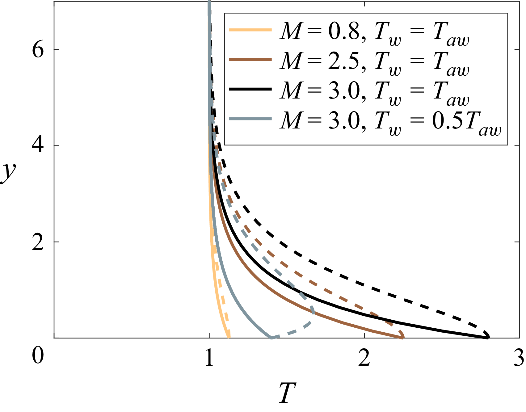

 ωi,max=maxα,βωi
 h
h ϕ
ϕ ϕ
ϕ M=4.2
M=4.2 ϕ
ϕ M=4.2
M=4.2 M=0.8
M=0.8 h
h M=0.8
M=0.8 hcrit
hcrit
 ωi,max=maxα,βωi
 h
h ϕ
ϕ h
h ϕ
ϕ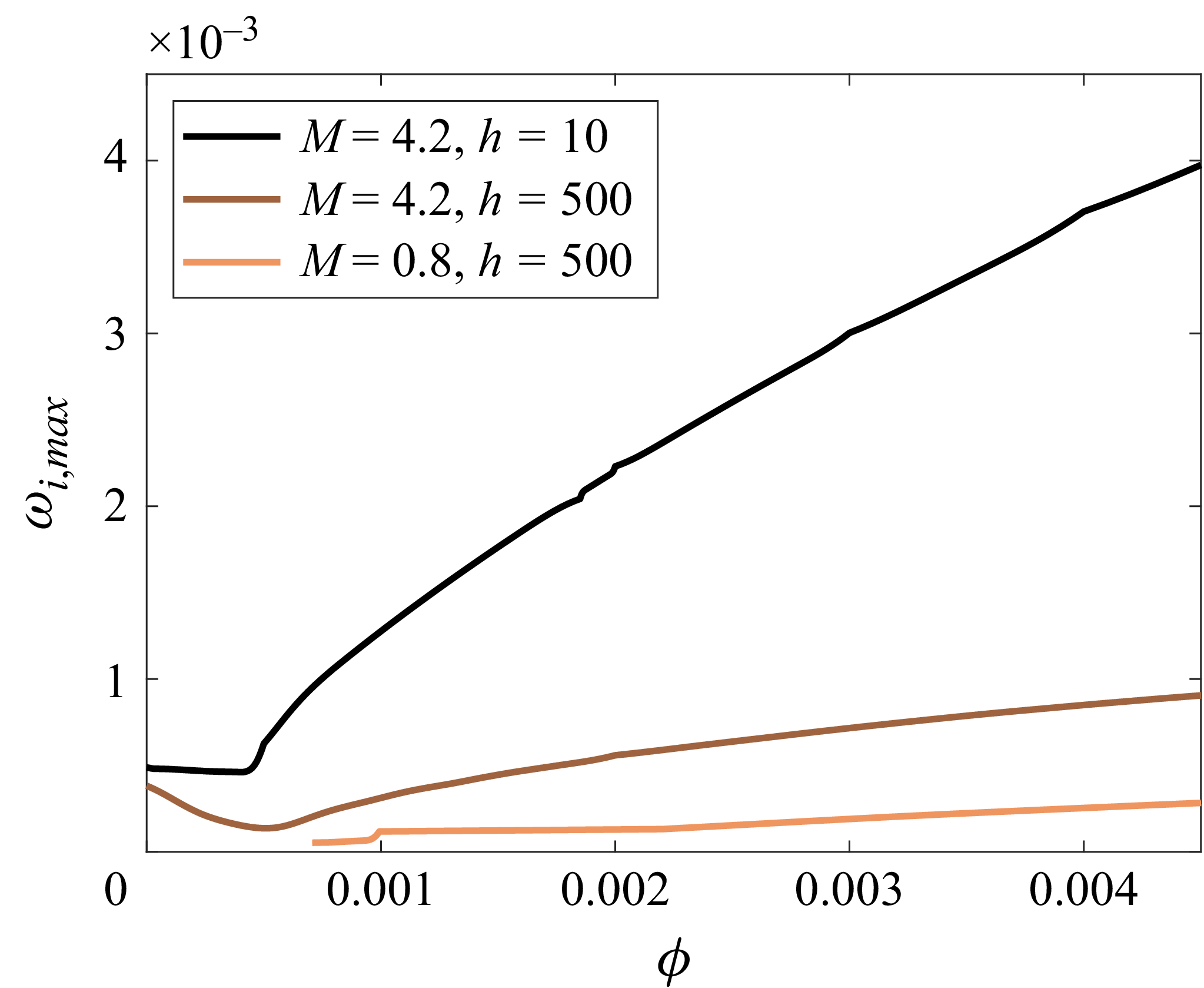
 ωi,max=maxα,βωi
 ϕ
ϕ M−h
M−h ϕ
ϕ
 ωi
ωi cx
cx α
α M=4.2
M=4.2 h=10
h=10 ϕ=0.002
 ϕ=0.1
ϕ=0.1 ϕ=0.3
ϕ=0.3 ⧫
⧫ cx=1−1/M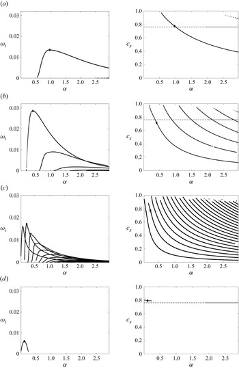
 ωi
ωi cx
cx α
α M=4.2
M=4.2 ϕ=0.1
ϕ=0.1 h=0.5
h=0.5 h=3
h=3 h=13
h=13 h=700
h=700 ⧫
⧫ cx=1−1/M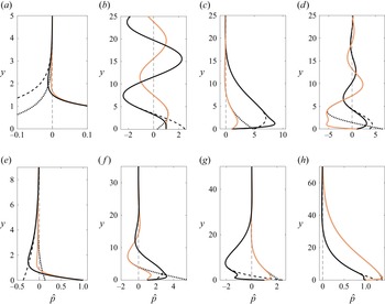
 p^
p^ (α,ω)
(α,ω) p^
p^ p^ff
p^ff α≈1.96
 ω≈1.72+0.0005i
 h=10,ϕ=0.0002
 α≈0.18
 ω≈0.08+0.0018i
 h=10,ϕ=0.3
 α≈0.33
 ω≈0.26+0.0277i
 h=10,ϕ=0.3
 α≈0.58
 ω≈0.39+0.0229i
 h=0.5,ϕ=0.1
 α≈0.97
 ω≈0.75+0.0135i
 h=3,ϕ=0.1
 α≈0.41
 ω≈0.29+0.0286i
 h=13,ϕ=0.1
 α≈0.25
 ω≈0.19+0.0171i
 h=700,ϕ=0.1
 α≈0.12
 ω≈0.10+0.0060i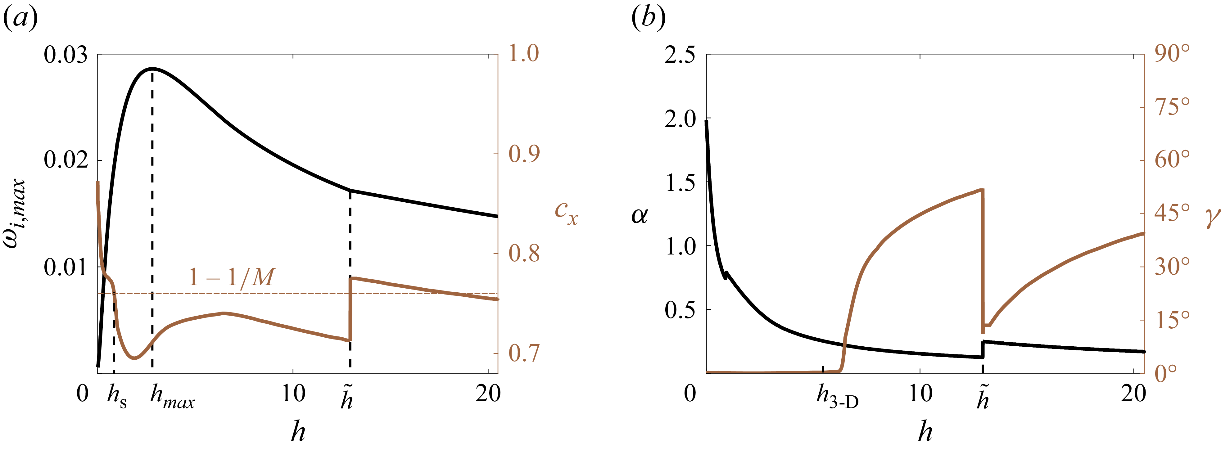
 α
α β
β h
h M=4.2
M=4.2 ϕ=0.1
ϕ=0.1 ωi,max
 cx
cx α
α γ
γ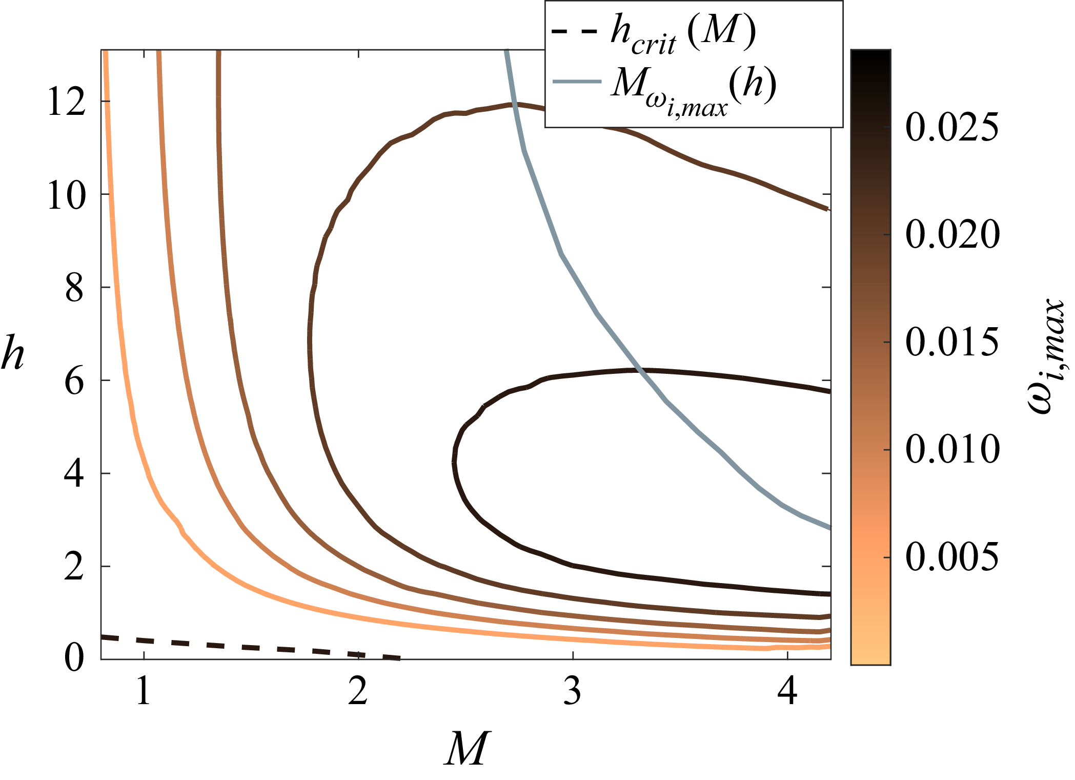
 ωi,max=maxα,βωi
 M
M h
h ϕ=0.1
ϕ=0.1 h
h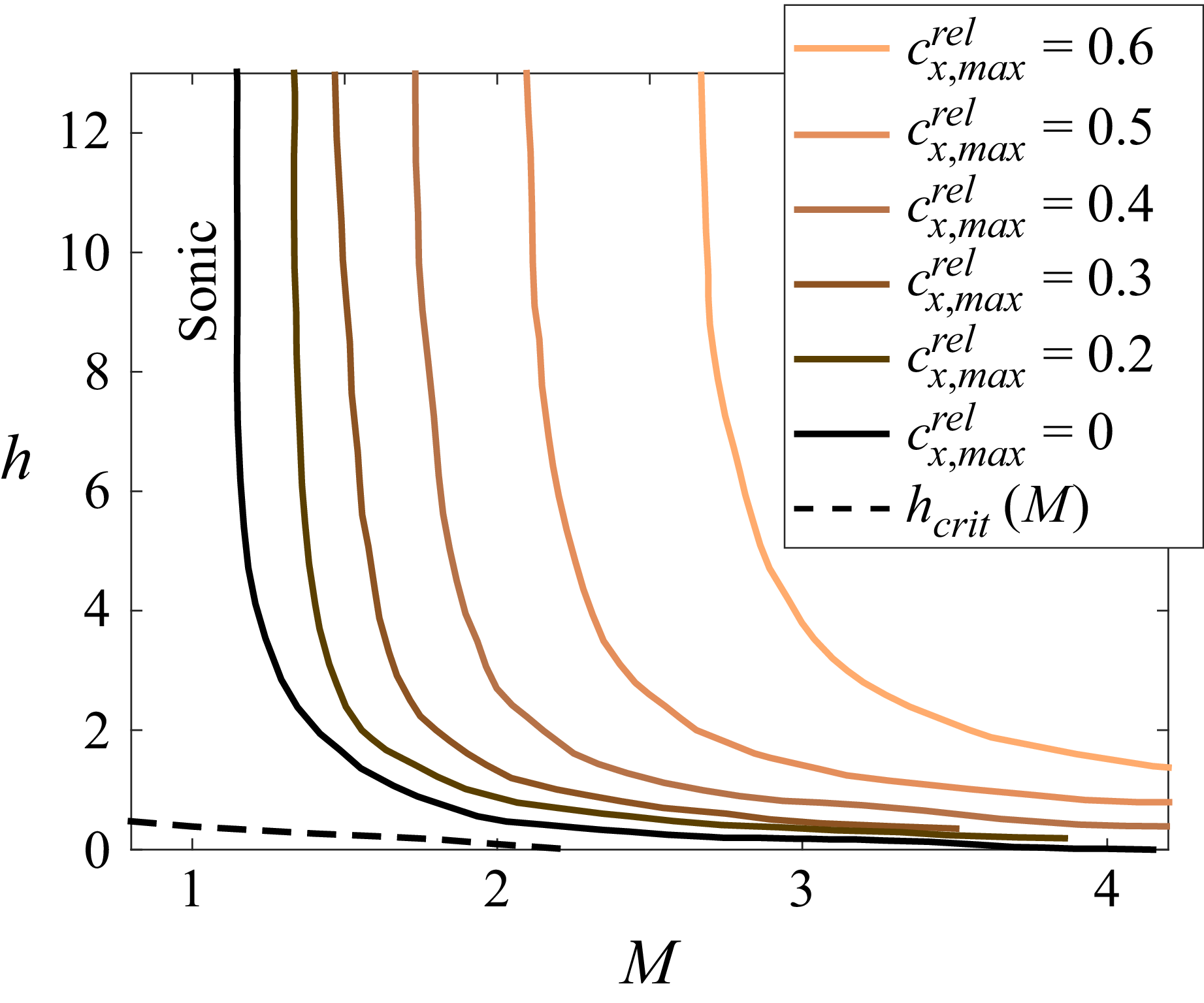
 cx,maxrel=maxα,β(1−1/M−cx)
 M
M h
h ϕ=0.1
ϕ=0.1 cx,maxrel>0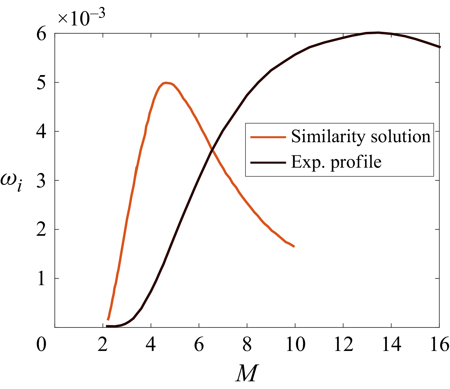
 M
M δ99
δ99
 Open access

