


1. Introduction
Faraday instability occurs when a horizontal liquid layer with a free surface is oscillated in a direction normal to the interface with an amplitude that exceeds a critical value. The instability manifests itself as interfacial waveforms of predictable wavelength that will either saturate or collapse, depending on the frequency of oscillation. The name of the instability derives from the experimental observations of Michael Faraday, who first described the ‘beautiful crispations’ formed in various fluid–air interfaces when a container housing a fluid is struck with a violin bow at different frequencies (Faraday Reference Faraday1831). These interfacial waveforms occur as a result of a resonance between the frequency at which the system is being excited and one or more natural frequencies of the system, which are governed by both fluid and geometric properties (Batson, Zoueshtiagh & Narayanan Reference Batson, Zoueshtiagh and Narayanan2013a ).
Qualitative pool boiling curve in Earth’s gravity, where $F$
is the heat flux and
$F$
is the heat flux and $\Delta T$
is the superheat, or the difference between the surface temperature and the boiling point of the liquid above; cf. Lienhard & Dhir (Reference Lienhard and Dhir1973).
$\Delta T$
is the superheat, or the difference between the surface temperature and the boiling point of the liquid above; cf. Lienhard & Dhir (Reference Lienhard and Dhir1973).

In the presence of gravity, buoyancy plays a central role in many convective heat transfer processes. Prior studies have shown that time-periodic modulation of gravity can suppress buoyancy-driven convective instabilities through resonance, or conversely destabilise otherwise buoyantly stable configurations (Gresho & Sani Reference Gresho and Sani1970; Gershuni & Lyubimov Reference Gershuni and Lyubimov1998; Shukla & Narayanan Reference Shukla and Narayanan2002). However, in reduced-gravity environments, where buoyancy-driven convection is negligible or absent, Faraday instability presents a promising alternative mechanism for enhancing heat transport. As an example, in the case of pool boiling, the shape of a characteristic boiling curve that depicts heat flux versus the temperature difference between a hot surface and the saturation temperature depends greatly on buoyancy (cf. figure 1). As the surface temperature increases, the dominant mechanism of heat transfer transitions from natural convection (region A) to nucleate boiling (region B) – characterised by steady bubble formation and detachment from the surface. The bubble flow increases until a critical heat flux is reached. This point, denoted CHF, was noted by Zuber (Reference Zuber1958) to represent the vapour outflow from the plate obstructing the returning liquid flow. Transition to lower heat flux occurs (region C) with increasing surface temperature until a vapour blanket covers the surface and significantly inhibits conductive heat transfer since the vapour’s thermal conductivity is much lower than that of the liquid. This point is known as the minimum heat flux, or MHF. Conduction continues through the vapour blanket and steadily rises as temperature increases, often until a burnout of the heater is observed (region D). In reduced-gravity conditions, there is no buoyancy forcing, thus there is no natural convection nor a mechanism by which bubbles can readily dislodge from the heating surface and commute to the liquid–vapour interface. Consequently, bubbles produce a film at lower temperatures than on Earth, causing a vapour lock and significant reduction in the efficiency of a boiling heat exchange system in space operations. The boiling curves for variable gravity systems were compared by Kim, Benton & Wisniewski (Reference Kim, Benton and Wisniewski2002) and exhibit this gravity dependence, where the critical heat flux is lowered and shifted to lower temperatures under low gravity. In response to this issue, several methods have been suggested to improve pool boiling in space environments.
A clear step to overcoming the challenge of early onset film formation during microgravity is to replace gravity’s role in the system. The use of electric fields is one such method (Patel et al. Reference Patel, Robinson, Seyed-Yagoobi and Didion2013), wherein a body force is applied to bubbles with ensuing flow that resembles natural convection. However, this can only be used with fluids with specific electrical properties such as R-123, a refrigerant. The use of forced flow boiling would be another way in which heat transfer could be improved, as in NASA’s Flow Boiling and Condensation Experiment, delivered to the International Space Station in 2021 (Mudawar et al. Reference Mudawar, Devahdhanush, Darges, Hasan, Nahra, Balasubramaniam and Mackey2023). Finally, multiple promising investigations concern the use of acoustic forcing (Park & Bergles Reference Park and Bergles1988; Chung Reference Chung1994; Hao, Oguz & Prosperetti Reference Hao, Oguz and Prosperetti2001) to provide body forces that can also drive bubbles from the surface.
While the above methods provide an opportunity to use two-phase heat transfer in microgravity operations, the main goal is to replace gravity-induced buoyancy with alternative means of flow generation and bubble removal. By contrast, the resonance effect of Faraday instability on enhanced heat transfer could lead to a method in which the unique fluid physics in reduced gravity can be utilised, rather than eliminated, thereby motivating the current study. In our work, we consider a layer of fluid with a free surface subject to a temperature gradient and oscillatory acceleration so as to induce resonance. We seek to determine how the enhancement of heat transfer changes as a function of gravity level and the interface deformation shape (waveform or mode). We will show by way of a reduced-order model that reduced gravity will substantially increase heat transfer when resonance-induced instability is employed. In addition, experiments done under Earth’s gravity reveal qualitative agreement with the theoretical predictions.
The paper is arranged as follows. In § 2, we present a mathematical model upon using a separation of length scales, and reveal the key dimensionless groups of interest. In § 3, the mathematical model is used to determine the effect of gravity on heat transfer using nonlinear simulations, which are preceded by a linear stability analysis that provides the necessary input parameters to incite the instability. We conclude the study with detailed experiments that show a significant increase in heat transfer resulting from the Faraday instability, and also show qualitative agreement with the observations made from nonlinear simulations. These findings and their importance are summarised in the last section of the paper.
2. The mathematical model
In the present study, the heat transfer and fluid instability are modelled in contexts where the depth of the fluid is less than the characteristic wavelength of instability and thus in the realm of the so-called ‘long-wave approximation’ (Kalliadasis et al. Reference Kalliadasis, Ruyer-Quil, Scheid and Velarde2011). The theoretical basis is parallel to much of the early work on falling liquid films, which incorporates a weighted residual method to the integral boundary layer model (cf. Ruyer-Quil & Manneville Reference Ruyer-Quil and Manneville1998; Rojas et al. Reference Rojas, Argentina, Cerda and Tirapegui2010; Bestehorn Reference Bestehorn2013; Dietze & Ruyer-Quil Reference Dietze and Ruyer-Quil2015).
The schematic representation of the model is shown in figure 2. The theoretical development of the model involves the following key assumptions.
-
(i) The upper fluid is hydrodynamically passive but thermally conductive.
-
(ii) The model is solved only in the $xz$
-plane, i.e. it is two-dimensional.
$xz$
-plane, i.e. it is two-dimensional. -
(iii) The height of the bottom fluid
$H$
is much less than its width
$W$
, leading to the long-wave approximation. -
(iv) Heat transfer is modelled using Newton’s law of cooling, and an infinite Biot number is assumed to simplify the final model. This implies negligible thermal resistance in the air layer, allowing the resonant flow to achieve the maximum possible heat transfer predicted by the model.
-
(v) All thermophysical properties are assumed independent of temperature, therefore the velocity fields are independent of the temperature field, while the latter is governed by both conduction and the velocity field (i.e. assuming one-way coupling).


The heat transfer system. A viscous fluid in contact with a passive fluid above is subject to a time-varying gravitational field while subjected to heating from above.

We note that a long-wave approximation assumes that the wavelength of interfacial disturbances is larger than the fluid depth, not merely that the container has a large horizontal extent $W$
. If the system is forced at frequencies that excite short-wavelength modes, then the model may no longer be valid. Therefore, a linear stability analysis should be performed first to confirm that the resulting wavelengths fall within the model’s range of applicability before proceeding with nonlinear simulations.
$W$
. If the system is forced at frequencies that excite short-wavelength modes, then the model may no longer be valid. Therefore, a linear stability analysis should be performed first to confirm that the resulting wavelengths fall within the model’s range of applicability before proceeding with nonlinear simulations.
We further note that the final two assumptions both independently eliminate the consideration of Marangoni convection. Marangoni convection occurs when there is a gradient of interfacial tension along the interface, which is driven by a temperature gradient and the temperature dependence of interfacial tension. The former is eliminated by effectively assuming an isothermal interface, and the latter is eliminated by assuming that all thermophysical properties are not functions of temperature.
The objective of the model is to forecast long-term heat flux and interface behaviour under specific fluid and geometric conditions, oscillation parameters and gravity levels. These predictions are then given physical interpretation in addition to being qualitatively compared with experimental data.
2.1. The governing equations and boundary conditions
The domain equations in the moving frame governing the fluid dynamics include the Navier–Stokes equations and the continuity equation, i.e.
 \begin{align}& \rho \left(\frac {\partial \boldsymbol{v}}{\partial t} + \boldsymbol{v} \boldsymbol{\cdot} \boldsymbol{\nabla} \boldsymbol{v}\right) = - \boldsymbol{\nabla} p + \mu\, \nabla ^2 \boldsymbol{v} - \rho \big (g + A \omega ^2 \cos (\omega t)\big ) \boldsymbol{k}\end{align}
and
 \begin{align}&\quad\,\boldsymbol{\nabla} \boldsymbol{\cdot} \boldsymbol{v} = 0,\end{align}
where the velocity field is denoted by $\boldsymbol{v}$
, the pressure field by
$\boldsymbol{v}$
, the pressure field by $p$
, the dynamic viscosity by
$p$
, the dynamic viscosity by $\mu$
, and density by
$\mu$
, and density by $\rho$
. The acceleration in the
$\rho$
. The acceleration in the $z$
-direction (indicated by unit vector
$z$
-direction (indicated by unit vector $\boldsymbol{k}$
) consists of gravity
$\boldsymbol{k}$
) consists of gravity $g$
, and the acceleration due to oscillation
$g$
, and the acceleration due to oscillation $A \omega ^2 \cos (\omega t)$
, where
$A \omega ^2 \cos (\omega t)$
, where $A$
denotes the shaking amplitude, and
$A$
denotes the shaking amplitude, and $\omega$
denotes the oscillation frequency expressed in radians per unit time.
$\omega$
denotes the oscillation frequency expressed in radians per unit time.
Added to the momentum and continuity equations is the energy conservation equation, which describes the temperature field $T$
, given by
$T$
, given by
 \begin{equation} \frac {\partial T}{\partial t} + \boldsymbol{v} \boldsymbol{\cdot} \boldsymbol{\nabla} T = \kappa\, \nabla ^2 T, \end{equation}
where the thermal diffusivity of the liquid is denoted by $\kappa$
, defined as
$\kappa$
, defined as $\kappa = {k_c}/{(\rho c_p)}$
, with
$\kappa = {k_c}/{(\rho c_p)}$
, with $k_c$
and
$k_c$
and $c_p$
the thermal conductivity and specific heat of the fluid, respectively.
$c_p$
the thermal conductivity and specific heat of the fluid, respectively.
The fluid is subject to no-slip and no-penetration at the flat bottom surface, thus we have $w=0=u$
at
$w=0=u$
at $z = 0$
, where
$z = 0$
, where $w$
and
$w$
and $u$
are the vertical and horizontal components of velocity, respectively. The bottom surface is at a constant temperature, i.e.
$u$
are the vertical and horizontal components of velocity, respectively. The bottom surface is at a constant temperature, i.e. $T = T_{cold}$
, so indicated as the fluid system is heated from above.
$T = T_{cold}$
, so indicated as the fluid system is heated from above.
The interfacial boundary conditions are comprised of a normal stress balance, a tangential stress balance, the no-mass transfer condition and Newton’s law of cooling. Thus we have the following.
The normal stress balance at $z = h(x,t)$
is
$z = h(x,t)$
is
 \begin{equation} \boldsymbol{n} \boldsymbol{\cdot} ({\unicode{x1D64F}} \boldsymbol{\cdot} \boldsymbol{n}) = - \gamma\, \boldsymbol{\nabla} _H \boldsymbol{\cdot} \boldsymbol{n}, \end{equation}
where $\boldsymbol{n}$
is the unit normal vector on the interface, in the positive
$\boldsymbol{n}$
is the unit normal vector on the interface, in the positive $z$
-direction,
$z$
-direction, $\unicode{x1D64F}$
is the total stress tensor,
$\unicode{x1D64F}$
is the total stress tensor, $\gamma$
is the interfacial tension, and
$\gamma$
is the interfacial tension, and $\boldsymbol{\nabla} _H$
is the horizontal gradient.
$\boldsymbol{\nabla} _H$
is the horizontal gradient.
The tangential stress balance at $z = h(x,t)$
is
$z = h(x,t)$
is
 \begin{equation} \boldsymbol{t}\boldsymbol{\cdot} ({\unicode{x1D64F}} \boldsymbol{\cdot} \boldsymbol{n}) = 0, \end{equation}
where $\boldsymbol{t}$
is the unit tangent vector on the interface, in the positive
$\boldsymbol{t}$
is the unit tangent vector on the interface, in the positive $x$
-direction.
$x$
-direction.
There is no flow across the interface at $z = h(x,t)$
, i.e.
$z = h(x,t)$
, i.e.
 \begin{equation} \boldsymbol{v} \boldsymbol{\cdot} \boldsymbol{n} = U, \end{equation}
where $U$
is the speed of the interface, given by
$U$
is the speed of the interface, given by
 \begin{equation} U=\frac {\dfrac{\partial {h}}{\partial {t}}}{(1+ \left(\dfrac{\partial h}{\partial x} \right)^2)^{1/2}}. \end{equation}
Newton’s law of cooling at $z = h(x,t)$
is
$z = h(x,t)$
is
 \begin{equation} - k_c\, \boldsymbol{\nabla} T \boldsymbol{\cdot} \boldsymbol{n} = - k_c \left (- \frac {\partial T}{\partial x} \frac {\partial h}{\partial x} + \frac {\partial T}{\partial z} \right ) \left (1+ \left (\frac {\partial h}{\partial x} \right )^2 \right )^{-{1}/{2}}= \alpha (T - T_{hot}), \end{equation}
where $\alpha$
represents the heat transfer coefficient at the interface.
$\alpha$
represents the heat transfer coefficient at the interface.
Characteristic scales for relevant variables used in the model.

2.2. Summary of scaled equations
Scaling is performed on the system using the characteristic scales shown in table 1, and the long-wave approximation is used to scale out small viscous terms in the governing equations using a small term $\delta = {H}/{W}$
(more detail is provided in Appendix A). A summary of the system of equations that remains after scaling according to the long-wave approximation is given below. Note that the variables
$\delta = {H}/{W}$
(more detail is provided in Appendix A). A summary of the system of equations that remains after scaling according to the long-wave approximation is given below. Note that the variables $p$
,
$p$
, $u$
,
$u$
, $w$
,
$w$
, $t$
,
$t$
, $x$
,
$x$
, $z$
,
$z$
, $\omega$
now represent scaled quantities. The important dimensionless groups that appear in the system of equations are given in table 2. Of note is the dimensionless acceleration
$\omega$
now represent scaled quantities. The important dimensionless groups that appear in the system of equations are given in table 2. Of note is the dimensionless acceleration $\Omega$
, dimensionless gravity
$\Omega$
, dimensionless gravity $G$
, capillary number
$G$
, capillary number $Ca$
, and Prandtl number
$Ca$
, and Prandtl number $Pr$
.
$Pr$
.
Relevant dimensionless groups appearing in the model.

The $x\hbox{-}$
momentum equation is
$x\hbox{-}$
momentum equation is
 \begin{equation} \delta \left (\frac {\partial u}{\partial t} + u \frac {\partial u}{\partial x} + w \frac {\partial u}{\partial z} \right ) = - \delta \frac {\partial p}{\partial x} + \frac {\partial ^2 u}{\partial z^2}, \end{equation}
and the $z$
-momentum equation is
$z$
-momentum equation is
 \begin{equation} \delta \frac {\partial p}{\partial z} = - \delta ( \Omega \cos (\omega t) + G), \end{equation}
where the velocity and pressure fields satisfy the continuity equation
 \begin{equation} \frac {\partial u}{\partial x}= - \frac {\partial w}{\partial z}. \end{equation}
The temperature field is governed by the energy equation
 \begin{equation} \delta\,\textit{Pr} \left (\frac {\partial \Theta }{\partial t} + u \frac {\partial \Theta }{\partial x} + w \frac {\partial \Theta }{\partial z} \right ) = \frac {\partial ^2 \Theta }{\partial z^2}. \end{equation}
These domain equations are subject to the following boundary conditions:
 \begin{align} u = w = \Theta = 0 & \,\quad\quad\qquad\qquad\text{at }z = 0, \end{align}
 \begin{align} \frac {\partial u}{\partial z} = 0 & \qquad\qquad \text{at }z = h(x,t), \end{align}
 \begin{align} - u \frac {\partial h}{\partial x} + w = \frac {\partial h}{\partial t} & \qquad\qquad \text{at }z = h(x,t), \end{align}
 \begin{align} \frac {\delta ^3}{Ca} \frac {\partial ^2 h}{\partial x^2} = - \delta p & \qquad\qquad \text{at }z = h(x,t),\\[6pt]\nonumber \end{align}
and
 \begin{align} \qquad\qquad\,\,\Theta = 1 & \qquad\qquad \text{at }z = h(x,t). \end{align}
The long-wave model is reduced to three dependent variables using the weighted residual integral boundary layer (WRIBL) method, as detailed in Appendix B. The WRIBL process involves integrating over the fluid depth, $z$
, with respect to suitable weight functions. This results in the system of equations below, with the following dependent variables: interface height
$z$
, with respect to suitable weight functions. This results in the system of equations below, with the following dependent variables: interface height $h(x,t)$
(distance from
$h(x,t)$
(distance from $z = 0$
to the interface), mean horizontal flow
$z = 0$
to the interface), mean horizontal flow $q(x,t) = \int _0^h u\, {\mathrm d}z$
, and the bottom-wall heat flux
$q(x,t) = \int _0^h u\, {\mathrm d}z$
, and the bottom-wall heat flux $F(x,t) = {(\partial T}/{\partial z)} |_{z=0}$
.
$F(x,t) = {(\partial T}/{\partial z)} |_{z=0}$
.
The momentum balance, serving as the evolution equation for mean horizontal flow $q(x,t)$
, is given by
$q(x,t)$
, is given by
 \begin{equation} \delta \left (\frac {\partial q}{\partial t} + \frac {17 q}{7h} \frac {\partial q}{\partial x} - \frac {9q^2}{7h^2} \frac {\partial h}{\partial x}\right ) = - \frac {5q}{2h^2} + \frac {5\delta h}{6} \left (\frac {\delta ^2}{Ca}\frac {\partial ^3 h}{\partial x^3} - (\Omega \cos (\omega t) + G) \frac {\partial h}{\partial x} \right ). \end{equation}
The evolution equation for the interface height $h(x,t)$
is derived by integrating the continuity equation over the fluid depth and using the kinematic and no-penetration conditions to obtain
$h(x,t)$
is derived by integrating the continuity equation over the fluid depth and using the kinematic and no-penetration conditions to obtain
 \begin{equation} \frac {\partial q}{\partial x} = - \frac {\partial h}{\partial t}. \end{equation}
Finally, the evolution equation for the bottom-wall heat flux $F(x,t)$
(and thereby the temperature field) is similarly created using a weighted residual method, to yield
$F(x,t)$
(and thereby the temperature field) is similarly created using a weighted residual method, to yield
 \begin{equation} \delta\, \textit{Pr} \left ( \frac {\partial F}{\partial t} + \frac {15}{14} \frac {q}{h} \frac {\partial F}{\partial x} + \frac {15}{14} \frac {F q}{h^2} \frac {\partial h}{\partial x} + \frac {5}{7h^2} \frac {\partial q}{\partial x} - \frac {27}{28} \frac {F}{h} \frac {\partial q}{\partial x} \right ) - \frac {10}{h^3} + 10 \frac {F}{h^2} = 0. \end{equation}
We refer to § 3.2 for details on how solutions are obtained to (2.14), (2.15) and (2.16).
3. The effect of gravity on heat transfer using nonlinear simulations
Gravity plays a significant role in the motion of a free fluid interface and therefore in the Faraday instability. A simple demonstration of its role can be observed in the equation for the natural frequency of an inviscid fluid with a free surface, explicitly defined in Benjamin & Ursell (Reference Benjamin and Ursell1954):
 \begin{equation} \omega _{nat} = \sqrt {\tanh {kH}\left (\frac {k^3 \gamma }{\rho } + k g\right )}, \end{equation}
where $k$
represents the wavenumber of a disturbance,
$k$
represents the wavenumber of a disturbance, $H$
is the height of the fluid,
$H$
is the height of the fluid, $\gamma$
is the surface tension,
$\gamma$
is the surface tension, $\rho$
is the density, and
$\rho$
is the density, and $g$
is the acceleration due to gravity. One can observe that, holding
$g$
is the acceleration due to gravity. One can observe that, holding $k$
constant, the natural frequency of a given waveform will decrease as gravity
$k$
constant, the natural frequency of a given waveform will decrease as gravity $g$
is reduced or eliminated. This was observed experimentally by Diwakar et al. (Reference Diwakar, Jajoo, Amiroudine, Matsumoto, Narayanan and Zoueshtiagh2018), where a significantly higher wavenumber
$g$
is reduced or eliminated. This was observed experimentally by Diwakar et al. (Reference Diwakar, Jajoo, Amiroudine, Matsumoto, Narayanan and Zoueshtiagh2018), where a significantly higher wavenumber $k$
was obtained in microgravity when compared to the same oscillation frequency and fluid geometry in ground-based experiments.
$k$
was obtained in microgravity when compared to the same oscillation frequency and fluid geometry in ground-based experiments.
The forecast difference in behaviour across gravity levels is primarily due to the fact that as gravity is reduced, interfacial tension becomes the only restoring force countering the forced oscillations imposed in exciting the Faraday instability. In this section, simulations are performed to gauge the effect of varying gravitational fields on the interface stability, the interface evolution and dynamics, and ultimately heat transfer improvement from the Faraday instability.
The system characterised in table 3 is subjected to gravitational and oscillation conditions specified in table 4 so that comparisons can be made across scenarios. That is, for the same fluid system subjected to some interfacial waveform (in this case one where there is one full wave spanning the interface), and the same relative amplitude and frequency of shaking, the flow and temperature dynamics are simulated and analysed.
Physical properties of the system used in comparing the Faraday instability in different gravitational environments.

Characteristic values for the simulation in comparing the Faraday instability in different gravitational environments.

3.1. Linear stability
Linear stability analysis gives theoretical predictions of the critical shaking amplitude $\Omega _c$
, which is used as an input in the nonlinear simulations. Defining
$\Omega _c$
, which is used as an input in the nonlinear simulations. Defining $h(x,t) = 1 + h'(x,t)$
,
$h(x,t) = 1 + h'(x,t)$
, $q(x,t) = q'(x,t)$
, and collecting prime terms, the governing WRIBL momentum equations (2.14) and (2.15) become
$q(x,t) = q'(x,t)$
, and collecting prime terms, the governing WRIBL momentum equations (2.14) and (2.15) become
 \begin{equation} \delta \frac {\partial q'}{\partial t} = - \frac {5}{2} q' + \delta \frac {1}{Ca} \frac {5}{6} \frac {\partial ^3 h'}{\partial x^3} - \delta \frac {5}{6} G \frac {\partial h'}{\partial x} - \delta \frac {5}{6} \frac {\partial h'}{\partial x} \Omega _c \cos (\omega t) \end{equation}
and
 \begin{equation} \frac {\partial q'}{\partial x} = - \frac {\partial h'}{\partial t}. \end{equation}
Taking the derivative ${\partial }/{\partial x}$
of (3.2) and replacing
${\partial }/{\partial x}$
of (3.2) and replacing ${\partial q'}/{\partial x}$
with
${\partial q'}/{\partial x}$
with $-{\partial h'}/{\partial t}$
via (3.3), we obtain
$-{\partial h'}/{\partial t}$
via (3.3), we obtain
 \begin{equation} \delta \frac {\partial ^2 h'}{\partial t^2} + \frac {5}{2} \frac {\partial h'}{\partial t} + \frac {5}{6} \frac {\delta ^3}{Ca} \frac {\partial ^4 h'}{\partial x^4} - \frac {5}{6} \delta \frac {\partial ^2 h'}{\partial x^2} (\Omega _c \cos (\omega t) + G)= 0 . \end{equation}
We then take the end conditions to be stress-free ( ${\partial h'}/{\partial x}=0$
at the vertical walls), and use a Floquet expansion to express
${\partial h'}/{\partial x}=0$
at the vertical walls), and use a Floquet expansion to express $h'$
as
$h'$
as $h' = \cos (k x) \sum _{n=-N}^{N} \hat {h}_n \exp (i n ({\omega }/{2})t)$
, using the identity
$h' = \cos (k x) \sum _{n=-N}^{N} \hat {h}_n \exp (i n ({\omega }/{2})t)$
, using the identity $\cos (\omega t) = {1}/{2} (\exp (i \omega t) + \exp (- i \omega t))$
to find a relationship between different frequency components
$\cos (\omega t) = {1}/{2} (\exp (i \omega t) + \exp (- i \omega t))$
to find a relationship between different frequency components $\hat {h}_n$
, i.e.
$\hat {h}_n$
, i.e.
 \begin{equation} - \frac {\omega ^2 n^2}{4} \hat {h}_n + \frac {5}{4} i n \omega \hat {h}_n + \frac {5}{6} \delta k^4 \hat {h}_n + \frac {5}{6} \frac {\delta ^3}{Ca} k^2 G \hat {h}_n -\frac {5}{12} \delta k^2 \Omega _c (\hat {h}_{n+2} + \hat {h}_{n-2}) = 0. \end{equation}
This is a problem with eigenvalue $\Omega _c$
and eigenvector
$\Omega _c$
and eigenvector $\hat {h_n}$
, noting that the accuracy increases with increasing ‘cut-off’
$\hat {h_n}$
, noting that the accuracy increases with increasing ‘cut-off’ $N$
. The problem takes the form
$N$
. The problem takes the form
 \begin{equation} {\unicode{x1D63C}} \hat {h} = \Omega _c {\unicode{x1D63D}} \hat {h}. \end{equation}
The eigenvalue $\Omega _c$
is calculated for a range of frequencies and parameters (fluid and geometric properties) that define the system to generate a stability threshold with a specific waveform denoted by its wavenumber
$\Omega _c$
is calculated for a range of frequencies and parameters (fluid and geometric properties) that define the system to generate a stability threshold with a specific waveform denoted by its wavenumber $k$
.
$k$
.
As an aside, one can determine the natural frequency of a given waveform by using (3.4) upon removing the forcing term, assuming $h'(x,t) = \hat {h}' \exp (\sigma t + ikx)$
, and solving for
$h'(x,t) = \hat {h}' \exp (\sigma t + ikx)$
, and solving for $\omega _{nat} = \textrm {Im}(\sigma )$
(noting that
$\omega _{nat} = \textrm {Im}(\sigma )$
(noting that $\sigma$
is complex) to find the expression
$\sigma$
is complex) to find the expression
 \begin{equation} \omega _{nat} = 2 \pi f_{nat} = \frac {1}{ \delta } \sqrt {\frac {5}{6} \delta k^2 \left (\frac {k^2 \delta ^2}{Ca} + G \right )-\frac {25}{16}}, \end{equation}
where the factor ${5}/{6}$
inside the radical arises from the low-order approximation made in the WRIBL method, and approaches unity with increasing order in
${5}/{6}$
inside the radical arises from the low-order approximation made in the WRIBL method, and approaches unity with increasing order in $\delta$
. It can be observed from (3.7) that the natural frequency is dependent on
$\delta$
. It can be observed from (3.7) that the natural frequency is dependent on $G$
. Shown in figure 3 is the stability threshold, expressed as dimensionless acceleration (the ratio of oscillation acceleration to Earth gravity
$G$
. Shown in figure 3 is the stability threshold, expressed as dimensionless acceleration (the ratio of oscillation acceleration to Earth gravity $g_e=9.8\ \mathrm m\ \mathrm s^{-2}$
) required to excite a waveform with wavelength of the container’s width (
$g_e=9.8\ \mathrm m\ \mathrm s^{-2}$
) required to excite a waveform with wavelength of the container’s width ( $k = 2 \pi$
) across the four gravity levels considered. The stability threshold is shown as a function of
$k = 2 \pi$
) across the four gravity levels considered. The stability threshold is shown as a function of ${f}/({f_{sub}})$
, where
${f}/({f_{sub}})$
, where $f_{sub}=2f_{nat}$
is the subharmonic resonant frequency, characterised by the interface oscillating one cycle for every two cycles of external oscillation. Plotting the threshold in this fashion allows one to better conceptualise the difference in stability across gravity levels around the subharmonic resonant frequency.
$f_{sub}=2f_{nat}$
is the subharmonic resonant frequency, characterised by the interface oscillating one cycle for every two cycles of external oscillation. Plotting the threshold in this fashion allows one to better conceptualise the difference in stability across gravity levels around the subharmonic resonant frequency.
To give a broader picture of the impact of gravity using linear stability, one can also plot the threshold of instability in terms of the threshold power (units $\text{W}\ \text{kg}^{-1}$
) needed to destabilise the interface, as shown in figure 4. This method of framing the system’s stability characteristics across gravity levels may give a more practical interpretation, since one may prefer to find the best heat transfer enhancement for an allotted power budget.
$\text{W}\ \text{kg}^{-1}$
) needed to destabilise the interface, as shown in figure 4. This method of framing the system’s stability characteristics across gravity levels may give a more practical interpretation, since one may prefer to find the best heat transfer enhancement for an allotted power budget.
The critical acceleration needed to destabilise the system with a waveform of $k = 2\pi$
(one full wave) described in table 3 in different gravitational environments as a function of the ratio
$k = 2\pi$
(one full wave) described in table 3 in different gravitational environments as a function of the ratio ${f}/{f_{sub}}$
, where
${f}/{f_{sub}}$
, where $f_{sub}$
is the subharmonic resonant frequency. At a given oscillation frequency, one is able to determine the threshold acceleration of shaking to produce a full wave at the interface using this linear stability analysis.
$f_{sub}$
is the subharmonic resonant frequency. At a given oscillation frequency, one is able to determine the threshold acceleration of shaking to produce a full wave at the interface using this linear stability analysis.

A comparison in linear stability framed in terms of specific power required to destabilise the system in different gravity levels. The parabolic sections represent different waveform responses on the interface at the point of instability. At a given oscillation frequency, one is able to determine the threshold power of shaking and the expected waveform response using this linear stability analysis.

3.2. Nonlinear simulation results
Nonlinear simulations are conducted for the four gravitational scenarios that produce wave height, flow and flux behaviour as functions of space and time. A snapshot of the waveforms at max deflection amplitude in varying $g$
environments is shown in figure 5.
$g$
environments is shown in figure 5.
A snapshot of the wave $k = 2\pi$
at the same relative oscillation amplitude and frequency across gravitational levels at the point of peak deflection (microgravity
$k = 2\pi$
at the same relative oscillation amplitude and frequency across gravitational levels at the point of peak deflection (microgravity $g = 0 \,\mathrm m\,\mathrm s^{-2}$
, Moon
$g = 0 \,\mathrm m\,\mathrm s^{-2}$
, Moon $g = 1.62 \,\mathrm m\,\mathrm s^-{^2}$
, Mars
$g = 1.62 \,\mathrm m\,\mathrm s^-{^2}$
, Mars $g = 3.2 \,\mathrm m\,\mathrm s^-{^2}$
, and Earth
$g = 3.2 \,\mathrm m\,\mathrm s^-{^2}$
, and Earth $g = 9.8 \,\mathrm m\,\mathrm s^-{^2}$
).
$g = 9.8 \,\mathrm m\,\mathrm s^-{^2}$
).

The nonlinear simulations are performed by solving (2.14), (2.15) and (2.16) via a Chebyshev spectral method (Guo, Labrosse & Narayanan Reference Guo, Labrosse and Narayanan2013) to resolve $x$
-dependency, and Mathematica’s NDSolve routine to solve coupled evolution equations at each nodal point. The
$x$
-dependency, and Mathematica’s NDSolve routine to solve coupled evolution equations at each nodal point. The $x$
-domain is re-scaled from
$x$
-domain is re-scaled from $[0,1]$
to
$[0,1]$
to $[-1,1]$
, and each of the dependent variables (heat flux
$[-1,1]$
, and each of the dependent variables (heat flux $F_n(t)$
, flow rate
$F_n(t)$
, flow rate $q_n(t)$
, and interface height
$q_n(t)$
, and interface height $h_n(t)$
) has nodal values at each point
$h_n(t)$
) has nodal values at each point $x_n$
, which are related to each other using
$x_n$
, which are related to each other using $x$
-derivative Chebyshev differential operators. Thus the system is defined by
$x$
-derivative Chebyshev differential operators. Thus the system is defined by $3(N + 1)$
total evolution equations, minus the equations used to implement the appropriate boundary conditions, that depend solely on the
$3(N + 1)$
total evolution equations, minus the equations used to implement the appropriate boundary conditions, that depend solely on the $3(N+1)$
nodal points.
$3(N+1)$
nodal points.
The $x$
-boundary conditions can depend upon the problem at hand, but for this system, we implement (i) free-slip (
$x$
-boundary conditions can depend upon the problem at hand, but for this system, we implement (i) free-slip ( ${\partial h}/{\partial x} = 0$
), (ii) no-flow (
${\partial h}/{\partial x} = 0$
), (ii) no-flow ( $q = 0$
), and (iii) insulated walls (
$q = 0$
), and (iii) insulated walls ( ${\partial T}/{\partial x} = 0$
) at the vertical walls. The initial conditions are accordingly defined for
${\partial T}/{\partial x} = 0$
) at the vertical walls. The initial conditions are accordingly defined for $t = 0$
and include a no-flow state
$t = 0$
and include a no-flow state $q(x,0) = 0$
, small waveform disturbance
$q(x,0) = 0$
, small waveform disturbance $h(x,0) = 1+0.01 \cos {kx}$
, and a flux governed by conduction in the base no-deflection state
$h(x,0) = 1+0.01 \cos {kx}$
, and a flux governed by conduction in the base no-deflection state $F(x,0) = 1$
.
$F(x,0) = 1$
.
The simulations are run until steady state is reached as shown by heat flux $F(x,t)$
, flow rate
$F(x,t)$
, flow rate $q(x,t)$
, and interface height
$q(x,t)$
, and interface height $h(x,t)$
behaviour. In this case, 100 spatial
$h(x,t)$
behaviour. In this case, 100 spatial $x$
-nodes are used, and the simulations are run for 200 forced oscillation cycles.
$x$
-nodes are used, and the simulations are run for 200 forced oscillation cycles.
In the results that follow, there are three primary methods in which the flow and flux behaviour characteristics are quantified, as listed below.
-
(i) The height of the so-called ‘anti-nodal’ point on the interface. The anti-node is the point that oscillates the greatest when the function is a pure cosine wave and gives a good one-dimensional interpretation of how strongly the interface is oscillating as a function of time. In this case with one full interfacial wave, the point
$x = 0$
behaves as the anti-node. -
(ii) The mean squared flow of the system. The mean squared flow is defined as the variable
$q(x,t)$
squared and integrated over
$x$
, resulting in a time-dependent function that characterises how vigorously the system is flowing. That is,(3.8)
\begin{equation} \overline {q^2} = \int _{-1}^{1} q^2(x,t)\, {\mathrm d}x. \end{equation}
-
(iii) The Nusselt number as a function of time. The variable
$F(x,t)$
is integrated over the bottom surface
$z = 0$
and divided by
$2$
(the integral value when the system is quiescent). The average long-term Nusselt number is shown for the different gravity levels in table 5.


The long-term Nusselt number at the bottom surface integrated over width for varying gravitational levels at equal relative magnitudes beyond the critical threshold ( $\Omega =1.3\Omega _c$
) and beyond the natural subharmonic frequency (
$\Omega =1.3\Omega _c$
) and beyond the natural subharmonic frequency ( $f=1.05 f_{sub}$
) for mode
$f=1.05 f_{sub}$
) for mode $k = 2 \pi$
in a 10 cSt silicone oil (
$k = 2 \pi$
in a 10 cSt silicone oil ( $\textit{Pr} = 83.3$
,
$\textit{Pr} = 83.3$
, $\delta = 0.08$
) system in contact with a passive upper layer.
$\delta = 0.08$
) system in contact with a passive upper layer.

Each metric can be used to gather information about the system. One notices from each of the graphs that they seem to generally share the same trend. The anti-node height generally correlates with the system’s flow magnitude, which correlates with an increase in flux.
The dynamics of the interface and the resulting flow are clearly distinguished across different gravitational levels. As was noted in the calculation of this system’s linear stability, the threshold amplitude and the threshold power needed to destabilise the interface generally increases with gravity. One may note in figure 10 that the amplitude of variation in heat transfer at the bottom wall as well as its time-averaged long-term value (table 5) increases as the stability of the interface decreases.
It is evident in figures 6, 7, 8 and 9 that the Nusselt number $Nu$
develops into a steady state well after the flow profile
$Nu$
develops into a steady state well after the flow profile $q^2(x,t)$
and the interface deflection
$q^2(x,t)$
and the interface deflection $h(x,t)$
. This result indicates that there is a lag time between the interface deflecting at its maximum amplitude and the flow adequately developing at the bottom wall, where the heat flux is calculated. This start-up condition of the instability could explain the temporary drop in heat transfer at the wall most strongly exhibited by the system in microgravity, shown in figure 6. This lag is also reduced by decreasing the Prandtl number
$h(x,t)$
. This result indicates that there is a lag time between the interface deflecting at its maximum amplitude and the flow adequately developing at the bottom wall, where the heat flux is calculated. This start-up condition of the instability could explain the temporary drop in heat transfer at the wall most strongly exhibited by the system in microgravity, shown in figure 6. This lag is also reduced by decreasing the Prandtl number $\textit{Pr}$
of the fluid as shown in figure 11. The 10 cSt silicone oil that was used in this work has a particularly high
$\textit{Pr}$
of the fluid as shown in figure 11. The 10 cSt silicone oil that was used in this work has a particularly high $\textit{Pr}$
of 83.3. As thermal diffusivity increases (and
$\textit{Pr}$
of 83.3. As thermal diffusivity increases (and $\textit{Pr}$
decreases), the fluid effectively becomes more conductive, and the heat transfer at the bottom wall is increasingly governed by distance to the interface (interface shape and deflection magnitude) rather than flow dynamics. In other words, the flux begins to synchronise more readily with the development of the interface and flow profile as the fluid becomes more conductive.
$\textit{Pr}$
decreases), the fluid effectively becomes more conductive, and the heat transfer at the bottom wall is increasingly governed by distance to the interface (interface shape and deflection magnitude) rather than flow dynamics. In other words, the flux begins to synchronise more readily with the development of the interface and flow profile as the fluid becomes more conductive.
Simulated dynamics of a 10 cSt silicone oil ( $\textit{Pr} = 83.3$
,
$\textit{Pr} = 83.3$
, $\delta = 0.08$
) system subject to microgravity (
$\delta = 0.08$
) system subject to microgravity ( $g = 0 \,\mathrm m\,\mathrm s^-{^2}$
) in contact with a passive upper layer that is oscillated at an amplitude beyond the critical threshold (
$g = 0 \,\mathrm m\,\mathrm s^-{^2}$
) in contact with a passive upper layer that is oscillated at an amplitude beyond the critical threshold ( $\Omega =1.3\Omega _c$
) and beyond the natural subharmonic frequency (
$\Omega =1.3\Omega _c$
) and beyond the natural subharmonic frequency ( $f=1.05 f_{sub}$
) such that the excited mode is
$f=1.05 f_{sub}$
) such that the excited mode is $k = 2 \pi$
. The dynamics is expressed using (a) the anti-node of the interface
$k = 2 \pi$
. The dynamics is expressed using (a) the anti-node of the interface $h({x}/{W} = 0.5, t)$
, (b) the
$h({x}/{W} = 0.5, t)$
, (b) the $x$
-integrated flow rate
$x$
-integrated flow rate $q^2$
, and (c)
$q^2$
, and (c) $Nu$
.
$Nu$
.

Simulated dynamics of a 10 cSt silicone oil ( $\textit{Pr} = 83.3$
,
$\textit{Pr} = 83.3$
, $\delta = 0.08$
) system subject to lunar gravity (
$\delta = 0.08$
) system subject to lunar gravity ( $g = 1.62 \,\mathrm m\,\mathrm s^-{^2}$
) in contact with a passive upper layer that is oscillated at an amplitude beyond the critical threshold (
$g = 1.62 \,\mathrm m\,\mathrm s^-{^2}$
) in contact with a passive upper layer that is oscillated at an amplitude beyond the critical threshold ( $\Omega =1.3\Omega _c$
) and beyond the natural subharmonic frequency (
$\Omega =1.3\Omega _c$
) and beyond the natural subharmonic frequency ( $f=1.05 f_{sub}$
) such that the excited mode is
$f=1.05 f_{sub}$
) such that the excited mode is $k = 2 \pi$
. The dynamics is expressed using (a) the anti-node of the interface
$k = 2 \pi$
. The dynamics is expressed using (a) the anti-node of the interface $h({x}/{W} = 0.5, t)$
, (b) the
$h({x}/{W} = 0.5, t)$
, (b) the $x$
-integrated flow rate
$x$
-integrated flow rate $q^2$
, and (c)
$q^2$
, and (c) $Nu$
.
$Nu$
.

Simulated dynamics of a 10 cSt silicone oil ( $\textit{Pr} = 83.3$
,
$\textit{Pr} = 83.3$
, $\delta = 0.08$
) system subject to Martian gravity (
$\delta = 0.08$
) system subject to Martian gravity ( $g = 3.2 \,\mathrm m\,\mathrm s^-{^2}$
) in contact with a passive upper layer that is oscillated at an amplitude beyond the critical threshold (
$g = 3.2 \,\mathrm m\,\mathrm s^-{^2}$
) in contact with a passive upper layer that is oscillated at an amplitude beyond the critical threshold ( $\Omega =1.3\Omega _c$
) and beyond the natural subharmonic frequency (
$\Omega =1.3\Omega _c$
) and beyond the natural subharmonic frequency ( $f=1.05 f_{sub}$
) such that the excited mode is
$f=1.05 f_{sub}$
) such that the excited mode is $k = 2 \pi$
. The dynamics is expressed using (a) the anti-node of the interface
$k = 2 \pi$
. The dynamics is expressed using (a) the anti-node of the interface $h({x}/{W} = 0.5, t)$
, (b) the
$h({x}/{W} = 0.5, t)$
, (b) the $x$
-integrated flow rate
$x$
-integrated flow rate $q^2$
, and (c)
$q^2$
, and (c) $Nu$
.
$Nu$
.

Simulated dynamics of a 10 cSt silicone oil ( $\textit{Pr} = 83.3$
,
$\textit{Pr} = 83.3$
, $\delta = 0.08$
) system subject to Earth’s gravity (
$\delta = 0.08$
) system subject to Earth’s gravity ( $g = 9.8 \,\mathrm m\,\mathrm s^-{^2}$
) in contact with a passive upper layer that is oscillated at an amplitude beyond the critical threshold (
$g = 9.8 \,\mathrm m\,\mathrm s^-{^2}$
) in contact with a passive upper layer that is oscillated at an amplitude beyond the critical threshold ( $\Omega =1.3\Omega _c$
) and beyond the natural subharmonic frequency (
$\Omega =1.3\Omega _c$
) and beyond the natural subharmonic frequency ( $f=1.05 f_{sub}$
) such that the excited mode is
$f=1.05 f_{sub}$
) such that the excited mode is $k = 2 \pi$
. The dynamics is expressed using (a) the anti-node of the interface
$k = 2 \pi$
. The dynamics is expressed using (a) the anti-node of the interface $h({x}/{W} = 0.5, t)$
, (b) the
$h({x}/{W} = 0.5, t)$
, (b) the $x$
-integrated flow rate
$x$
-integrated flow rate $q^2$
, and (c)
$q^2$
, and (c) $Nu$
.
$Nu$
.

The Nusselt number at the bottom surface integrated over width as a function of time for varying gravitational levels: (a) microgravity, (b) lunar gravity, (c) Martian gravity, and (d) Earth gravity, at equal relative magnitudes beyond the critical threshold ( $\Omega =1.3\Omega _c$
) and beyond the natural subharmonic frequency (
$\Omega =1.3\Omega _c$
) and beyond the natural subharmonic frequency ( $f=1.05 f_{sub}$
) for mode
$f=1.05 f_{sub}$
) for mode $k = 2 \pi$
in a 10 cSt silicone oil (
$k = 2 \pi$
in a 10 cSt silicone oil ( $\textit{Pr} = 83.3$
,
$\textit{Pr} = 83.3$
, $\delta = 0.08$
) system in contact with a passive upper layer.
$\delta = 0.08$
) system in contact with a passive upper layer.

The Nusselt number at the bottom surface integrated over width as a function of time with increasing thermal diffusivity (holding all other properties constant) at equal relative magnitudes beyond the critical threshold ( $\Omega =1.3\Omega _c$
) and beyond the natural subharmonic frequency (
$\Omega =1.3\Omega _c$
) and beyond the natural subharmonic frequency ( $f=1.05 f_{sub}$
) for mode
$f=1.05 f_{sub}$
) for mode $k = 2 \pi$
in a 10 cSt silicone oil system of
$k = 2 \pi$
in a 10 cSt silicone oil system of $\delta = 0.08$
in contact with a passive upper layer, in microgravity (
$\delta = 0.08$
in contact with a passive upper layer, in microgravity ( $g = 0$
). For the purposes of data comparison, a moving cycle-based average was used.
$g = 0$
). For the purposes of data comparison, a moving cycle-based average was used.

The analysis shows that gravitational levels significantly influence the interface dynamics and flow behaviour. The observed lag between maximum interface deflection and steady-state flow underscores an important characteristic of the heat transfer process during start-up, and demonstrates a complex interaction between the interface and the bottom wall. Simulation results also support the finding from linear stability analysis that shows, in general, that decreasing the gravity level destabilises the interface and leads to greater heat transfer.
4. The experimental study and discussion
4.1. Experimental set-up
Experiments in this work were completed using an oscillator where a fluid-containing cell is allowed to shake at a prescribed amplitude and frequency. The set-up is shown in figure 12. The figure depicts a water circuit whereby the temperature gradient was set. The cell was subjected to a gravitationally stable temperature gradient (heated from above) to minimise any natural convection that could affect heat flux measurements. The cell’s horizontal walls were held at constant temperature using the water circuits.
The experimental set-up consisting of an oscillator used to excite and monitor the Faraday instability in a fluid-containing cell hooked up to two temperature-controlled fluid loops. See the supplementary movie available at https://doi.org/10.1017/jfm.2025.10415 for the depiction of the experiment in action.

Figure 12 shows a diagram of the heat transfer cell used to monitor the heat transfer performance during the Faraday instability. Two heat flux sensors (FLUXTEQ PHFS-01) were used on the top and bottom surfaces for redundancy purposes and to ensure minimisation of heat losses in the lateral direction. Four T-type thermocouples were used to monitor the temperature of the upper and lower surfaces. The set-up was fastened to the oscillator and visualised with a camera in a fixed frame (i.e. not oscillating with the fluid cell). The cell and heat baths were constructed using 3-D-printed SLA transparent resin from FormLabs and a small acrylic window for fluid visualisation, with a 5 mm copper plate on the top and bottom serving as the conductive interface between flow loop and cell. The cell was illuminated with an LED back-light.
4.2. Experimental methods
Fluid (10 cSt silicone oil) was injected into a cell port with a volume calculated from the desired liquid height. An amplitude threshold generated by linear stability analysis as described in § 3.1 was used to assist in the experimental determination of threshold amplitude and frequency to excite the desired interfacial waveform.
The experiments measured the long-term heat flux and interfacial behaviour of two different waveforms, which can be selectively activated by changing the frequency of oscillation as determined by theoretical predictions. One frequency was selected for each waveform in this work, and the threshold oscillation amplitude was determined by iterating between amplitudes of instability and stability (cf. Batson et al. (Reference Batson, Zoueshtiagh and Narayanan2013b) for a comprehensive process description of experimental threshold determination for a given oscillation frequency).
Upon identifying the threshold oscillation amplitude, the system is allowed to return to rest (no oscillations) until a steady-state thermal profile is observed. The steady-state heat flux and temperature delta between top and bottom walls is used as the base-state reference for purposes of Nusselt number calculation. The system is then oscillated at an amplitude beyond the threshold amplitude until steady state is reached, which typically took 5–10 min. The system is allowed to come to rest after oscillating, reach steady state again while at rest, and subsequently oscillated at a yet higher amplitude, following the same procedure. This was repeated in a step-wise fashion until approximately 60 % above the observed critical threshold amplitude.
The interface was visualised in a fixed frame via high-speed imaging throughout the course of the oscillations. In other words, the camera was not oscillating along with the cell. The recording of the set-up in the fixed frame allows one to measure the amplitude and frequency of shaking through image analysis. By using a scale of known length (the thickness of the cell in this case), one can verify the amplitude of shaking used in the experiment, as illustrated in figure 13. The oscillation frequency is also verified by generating a space–time diagram extracted from an oscillation video and measuring the period of oscillation based on the frame rate of the camera, as visualised in figure 14. Experiments were operated at a single frequency while varying the amplitude between trials of oscillation. This allows for the motor to be run at a constant voltage throughout the experiment, and the frequency measurement is thus less sensitive to user error.
Determination of shaking amplitude through image analysis relies on scaling the image to a known length – in this case, the thickness of the cell, which is 9 mm.

Determination of frequency through image analysis is done via a space–time diagram depicting movement in the shaking direction, where each pixel across the $x$
-axis represents a video frame, and the
$x$
-axis represents a video frame, and the $y$
-direction is a specific line of pixels that spans the fluid interface. The frame rate
$y$
-direction is a specific line of pixels that spans the fluid interface. The frame rate $fps$
of the video and the number of frames per cycle
$fps$
of the video and the number of frames per cycle $N$
are needed to measure the oscillation frequency
$N$
are needed to measure the oscillation frequency $f$
using the formula
$f$
using the formula $f ={(fps)}/{N}$
.
$f ={(fps)}/{N}$
.

4.3. The effect of instability wavelength
In the absence of an experimental environment where the gravity can be varied, the legitimacy of the model in predicting the heat transfer improvement from the Faraday instability was supported with a set of experiments in a fluid system described by table 6 to compare the predictions of the model for different interface shapes, or modes. This was a practical parameter to test and compare, as the engineering applications of such a technology would centre around the question: what is the optimal interface shape, and consequently, how should the system be oscillated to achieve the maximum possible increase in heat transfer?
Physical properties of the system used in experiments and associated simulations. Note that these are not the same cell dimensions as used in the gravitational simulations.

The linear stability of the experimental system in the frequency range where $k = 2\pi$
and
$k = 2\pi$
and $k = 3\pi$
are the instability waveforms at onset. It is plotted as threshold amplitude in this case to provide a helpful guide for setting the experimental oscillation amplitude in searching for the point of instability.
$k = 3\pi$
are the instability waveforms at onset. It is plotted as threshold amplitude in this case to provide a helpful guide for setting the experimental oscillation amplitude in searching for the point of instability.

4.3.1. Experimental results
As discussed in § 4.2, the threshold of instability was determined for both two and three half-wave disturbances, respectively. In both cases, the threshold of instability was noted to be significantly different in experiment than what was predicted using the linear stability model, as shown in table 7. This observation has been made in Ward, Zoueshtiagh & Narayanan (Reference Ward, Zoueshtiagh and Narayanan2019) and has contributed to the non-idealities of boundary condition physics in finite rectangular geometries. This is accentuated in this case because, in addition to having relatively small horizontal extent, the fluid height was of the order of the interface deflection.
Experimental oscillation parameters used in Faraday heat transfer experiments and analogous simulations with different interface waveforms.

The experiments conducted in this work observed long-term behaviour of two waveforms in a rectangular geometry (figure 16) and compared their respective long-term Nusselt numbers. The heat transfer coefficient $\beta$
was used to derive the Nusselt number, which was calculated from experimental data using the equation
$\beta$
was used to derive the Nusselt number, which was calculated from experimental data using the equation
 \begin{equation} \beta = \frac {F}{T_{hot}-T_{cold}}. \end{equation}
The heat flux $F$
was determined by heat flux sensors, while the temperature difference was determined by the redundant temperature sensors on the top and bottom walls of the cell. The Nusselt number was then determined with reference to the steady state when the cell was not oscillating, using (4.2):
$F$
was determined by heat flux sensors, while the temperature difference was determined by the redundant temperature sensors on the top and bottom walls of the cell. The Nusselt number was then determined with reference to the steady state when the cell was not oscillating, using (4.2):
 \begin{equation} Nu=\frac {\beta _{ss, \textit{oscillating}}}{\beta _{ss,\textit{fixed}}}. \end{equation}
The results are shown in figure 17. The heat transfer improvement for the one full wave disturbance ( $k = 2\pi$
) was observed to be superior to the heat transfer improvement for the three half-wave disturbance (
$k = 2\pi$
) was observed to be superior to the heat transfer improvement for the three half-wave disturbance ( $k = 3\pi$
) as a function of relative amplitude above the instability threshold.
$k = 3\pi$
) as a function of relative amplitude above the instability threshold.
The two waveforms ( $k = 2\pi$
and
$k = 2\pi$
and $k = 3\pi$
, referred to as modes (
$k = 3\pi$
, referred to as modes ( $2,0$
) and (
$2,0$
) and ( $3,0$
), respectively) in a rectangular geometry in their theoretical form (
$3,0$
), respectively) in a rectangular geometry in their theoretical form ( $\cos(kx)$
) compared to what was observed in experiment.
$\cos(kx)$
) compared to what was observed in experiment.

A comparison of experimental long-term Nusselt numbers for two different waveforms in a 10 cSt silicone oil system as a function of the relative amplitude above the critical threshold.

4.3.2. Simulation results
A total of 240 nodes in the $x$
-direction are used to approximate the shape of the interface, and the numerical model used in § 3.2 is run until steady state is reached. This steady state typically takes approximately 200 oscillation cycles, but decreases as oscillation amplitude is increased. Therefore the simulation is run for fewer total cycles as amplitude is increased to minimise total computation time.
$x$
-direction are used to approximate the shape of the interface, and the numerical model used in § 3.2 is run until steady state is reached. This steady state typically takes approximately 200 oscillation cycles, but decreases as oscillation amplitude is increased. Therefore the simulation is run for fewer total cycles as amplitude is increased to minimise total computation time.
As seen in figure 18, the simulation results show qualitative agreement with the experiment with regard to the waveforms $k = 2 \pi$
and
$k = 2 \pi$
and $k = 3\pi$
(one full wave and three half-wave disturbances, respectively), in that the longer wavelength disturbance displays better overall heat transfer improvement as a function of relative oscillation amplitude above the critical amplitude threshold. This is supported by the small discrepancy in wave amplitudes at 10 % above the critical threshold, as shown in figure 19.
$k = 3\pi$
(one full wave and three half-wave disturbances, respectively), in that the longer wavelength disturbance displays better overall heat transfer improvement as a function of relative oscillation amplitude above the critical amplitude threshold. This is supported by the small discrepancy in wave amplitudes at 10 % above the critical threshold, as shown in figure 19.
A comparison of simulation Nusselt numbers for two different waveforms in a 10 cSt silicone oil system as a function of the relative amplitude above the critical threshold.

A comparison of the long-term interface deflection observed in simulation for (a) one full wave and (b) three half-wave disturbances in a 10 cSt silicone oil system at 10 % above the critical threshold, at the beginning of the cycle ( $t = n T$
) and halfway through a cycle (
$t = n T$
) and halfway through a cycle ( $t = (n + {1}/{2})T$
), where
$t = (n + {1}/{2})T$
), where $n$
is any integer, and
$n$
is any integer, and $T$
is the period of oscillation.
$T$
is the period of oscillation.

It is important to note that in practical terms, the comparison between the two waveforms can be analysed in various ways depending on the system constraints. If instead of plotting the data in terms of relative amplitude, one considers the long-term Nusselt number as a function of specific power (as seen in figure 20), one may arrive at the conclusion that the three half-wave disturbance may be the most optimal if the system is power-limited.
A comparison of the heat transfer performance for two waveforms ( $k = 2\pi$
and
$k = 2\pi$
and $k = 3\pi$
) when looked at in terms of specific power of oscillation, defined as
$k = 3\pi$
) when looked at in terms of specific power of oscillation, defined as $P = A^2 \omega ^3$
, for experimental and simulation results. The inset highlights the relationship between simulation results, which had much lower Nusselt number than observed in experiment.
$P = A^2 \omega ^3$
, for experimental and simulation results. The inset highlights the relationship between simulation results, which had much lower Nusselt number than observed in experiment.

A quantitative estimate of the relationship between the relative wave height ${a}/{H}$
and the resultant Nusselt number using a simple conduction-only model of the upper fluid and an isothermal lower fluid.
${a}/{H}$
and the resultant Nusselt number using a simple conduction-only model of the upper fluid and an isothermal lower fluid.

A significant difference between experimental observations and simulation predictions is noted in the Nusselt number. Experimentally determined Nusselt numbers in terrestrial gravity conditions are as high as 4.5, while simulations yield a maximum value of approximately 1.01. High-speed video analysis of the experiments reveals that the interface impinged upon the upper and lower walls, which is believed to be a primary cause of discrepancy between model and experiment.
4.4. Comparisons between simulation and experiment
The first source of discrepancy between model and experiment is the magnitude and complexity of the interface dynamics, resulting from the omission of key inertial terms in the momentum equations, and assumption of a two-dimensional, continuously differentiable interface shape. As a result, the model predicts relatively small ( $\approx0.5 \ \rm mm$
) interface deflections, while high-speed imaging reveals experimental interface amplitudes approaching the full fluid depth (
$\approx0.5 \ \rm mm$
) interface deflections, while high-speed imaging reveals experimental interface amplitudes approaching the full fluid depth ( $\approx4.5 \ \rm mm$
), leading in some cases to impingement on the upper and lower walls. To estimate the heat transfer impact of this underprediction at first order, assuming conduction-only improvement as a result of the increased interface height, a simple model is developed herein.
$\approx4.5 \ \rm mm$
), leading in some cases to impingement on the upper and lower walls. To estimate the heat transfer impact of this underprediction at first order, assuming conduction-only improvement as a result of the increased interface height, a simple model is developed herein.
We consider two fluids of equal height $H$
, of width
$H$
, of width $W=1$
, where the fluid interface height
$W=1$
, where the fluid interface height $h$
is oscillating as
$h$
is oscillating as $h(x,t) = H + a \cos (2 \pi x) \cos (2 \pi t)$
. Assuming a well-mixed bottom fluid such that it is isothermal everywhere including the interface, the cycle-averaged heat transfer (per unit depth into the page) between the interface and the upper wall would be given as
$h(x,t) = H + a \cos (2 \pi x) \cos (2 \pi t)$
. Assuming a well-mixed bottom fluid such that it is isothermal everywhere including the interface, the cycle-averaged heat transfer (per unit depth into the page) between the interface and the upper wall would be given as
 \begin{equation} Q = k_c\, \Delta T \int _0^1 \int _0^1 \frac {1}{H-a \cos (2 \pi x) \cos (2 \pi t)}\, \mathrm{d}x\, \mathrm{d}t. \end{equation}
With the base state heat transfer defined as $Q_0 = {(k_c \Delta T)}/{H}$
, the Nusselt number would therefore be given as
$Q_0 = {(k_c \Delta T)}/{H}$
, the Nusselt number would therefore be given as
 \begin{equation} Nu = \frac {Q}{Q_0} = \int _0^1 \int _0^1 \frac {1}{(1-({a}/{H}) \cos (2 \pi x) \cos (2 \pi t))}\, \mathrm{d}x\, \mathrm{d}t. \end{equation}
One can see by inspecting the integral that the time-averaged Nusselt number is dependent on the relative amplitude of the wave. (In fact, it can be shown via Taylor series expansion of the integrand to increase monotonically as a function of wave amplitude.) This behaviour is shown in figure 21. In the case of simulation, ${a}/{H} \approx 0.1$
, predicting a Nusselt number of approximately 1.0025. For experiment, however,
${a}/{H} \approx 0.1$
, predicting a Nusselt number of approximately 1.0025. For experiment, however, ${a}/{H} \approx 1$
, which therefore is predicted to lead to a Nusselt number of approximately 1.56. As intuition would suggest, this calculation is more appropriate for a gently deflecting interface and therefore would underpredict heat transfer from mixing in the upper fluid and impingement on the wall for a highly deflecting interface, but this calculation demonstrates that the nonlinear evolution of the interface is a significant contributor to the discrepancy between simulation and experiment.
${a}/{H} \approx 1$
, which therefore is predicted to lead to a Nusselt number of approximately 1.56. As intuition would suggest, this calculation is more appropriate for a gently deflecting interface and therefore would underpredict heat transfer from mixing in the upper fluid and impingement on the wall for a highly deflecting interface, but this calculation demonstrates that the nonlinear evolution of the interface is a significant contributor to the discrepancy between simulation and experiment.
The second key contributor to discrepancies between theory and experiment is the difference in threshold instability between the two scenarios. The experimental onset of Faraday instability occurs at significantly higher oscillation amplitudes than predicted by the model, largely due to additional dissipation mechanisms (e.g. meniscus waves, sidewall drag) not captured due to the assumed stress-free boundary conditions of the simulation domain (Ward et al. Reference Ward, Zoueshtiagh and Narayanan2019). This discrepancy leads to a striking difference in specific power input: as shown in figure 20, the experiment requires up to an order of magnitude greater specific power (e.g. 3.5 versus 0.5 W kg–1) to reach the instability threshold for a given waveform. More power available to the system permits a more vigorous flow state and therefore better mixing upon reaching instability, and better heat transfer performance.
To demonstrate this argument quantitatively, we present a scaling argument as follows. Recall that specific power is defined here as $P = A^2\omega ^3$
. For the purposes of this calculation, the velocity scale is assumed to be
$P = A^2\omega ^3$
. For the purposes of this calculation, the velocity scale is assumed to be $\bar {v} = \omega H$
. The Reynolds number
$\bar {v} = \omega H$
. The Reynolds number $Re$
can therefore be defined as
$Re$
can therefore be defined as
 \begin{equation} Re = \frac {\bar {v} H}{\nu } = \frac {A \omega }{\nu } = \frac {H}{\nu } \left (\frac {P}{\omega ^2}\right )^{\tfrac{1}{2}}. \end{equation}
The ratio of $Re$
between experiment and simulation can then be inferred, taking example notional points from figure 20 as
$Re$
between experiment and simulation can then be inferred, taking example notional points from figure 20 as $P_{exp} = 3.5\,\rm {W}\,{kg}^{-1}$
,
$P_{exp} = 3.5\,\rm {W}\,{kg}^{-1}$
, $P_{sim} = 0.5\,\rm {W}\,{kg}^{-1}$
, to obtain
$P_{sim} = 0.5\,\rm {W}\,{kg}^{-1}$
, to obtain
 \begin{equation} \frac {Re _{exp}}{Re _{sim}} \sim \left (\frac {P_{exp}}{P_{sim}}\right )^{\tfrac{1}{2}} = \left (\frac {3.5\ {\rm W}\ {\rm kg}^{-1}}{0.5\ {\rm W}\ {\rm kg}^{-1}}\right )^{\tfrac{1}{2}} \approx 2.65. \end{equation}
The connection between the Nusselt number and the Reynolds number can be estimated as following a relationship akin to $Nu \sim Re ^n$
, where
$Nu \sim Re ^n$
, where $n$
is an experimentally determined factor. Taking the work of Chen, Chen & Chen (Reference Chen, Chen and Chen1997) and Chen & Chen (Reference Chen and Chen1998) as a conservative analogue case reporting
$n$
is an experimentally determined factor. Taking the work of Chen, Chen & Chen (Reference Chen, Chen and Chen1997) and Chen & Chen (Reference Chen and Chen1998) as a conservative analogue case reporting $n = 0.5$
, the inferred Nusselt number ratio between experiment and simulation would be
$n = 0.5$
, the inferred Nusselt number ratio between experiment and simulation would be $2.65^{0.5} \approx 1.6$
, indicating that the nearly order of magnitude difference in specific power would be expected to drive a significant difference in heat transfer from mixing.
$2.65^{0.5} \approx 1.6$
, indicating that the nearly order of magnitude difference in specific power would be expected to drive a significant difference in heat transfer from mixing.
In addition to the above, the Biot number was assumed to be infinite in the mathematical model. This was done to provide an ‘upper bound’ performance and also eliminate any consideration of any Marangoni impacts. In reality, the Biot number of the experiment would likely be of the order of the ratio ${k_{air}}/{k_{oil}} \approx 0.1$
, considering equal fluid heights. This is, of course, not infinite, and would reduce our ability to compare results between simulation and experiment. However, considering (i) infinite Biot number would be an optimistic, high-performance case, and (ii) the fact that experimental measurements yielded much higher heat transfer than simulation, this Biot number assumption was not deemed to have a significant impact on the agreement between theory and experiment.
${k_{air}}/{k_{oil}} \approx 0.1$
, considering equal fluid heights. This is, of course, not infinite, and would reduce our ability to compare results between simulation and experiment. However, considering (i) infinite Biot number would be an optimistic, high-performance case, and (ii) the fact that experimental measurements yielded much higher heat transfer than simulation, this Biot number assumption was not deemed to have a significant impact on the agreement between theory and experiment.
As outlined here, the discrepancies observed between simulation and experiment highlight the utility of future models to include higher-order approximations to better capture the dynamics of interface motion, thereby reducing the divergence between predictions and experimental results. Specifically, the large values of the dimensionless groups for gravitational and oscillatory acceleration in this system ( $G$
and
$G$
and $\Omega$
) suggest that the inertial effects are too strong to permit a simple parabolic velocity profile. A more comprehensive model with additional parameters would serve to better capture the nonlinear evolution of the system. For instance, the incorporation of partial slip conditions at the boundaries could improve the model’s representation of the system dynamics and linear stability prediction.
$\Omega$
) suggest that the inertial effects are too strong to permit a simple parabolic velocity profile. A more comprehensive model with additional parameters would serve to better capture the nonlinear evolution of the system. For instance, the incorporation of partial slip conditions at the boundaries could improve the model’s representation of the system dynamics and linear stability prediction.
5. Summary
This study uses a model based on a weighted residual integral boundary layer method to predict heat transfer enhancement in a container exposed to forced oscillations in different gravitational environments, with the amplitude of oscillation exceeding the critical threshold for Faraday instability. Through linear stability analysis and nonlinear simulations across different gravity conditions, the model shows that the Nusselt number generally increases as the gravitational field decreases for a given waveform above the instability threshold.
Experimental results under Earth’s gravity confirm that the Faraday instability significantly boosts heat transfer across fluid interfaces. Moreover, the time-averaged Nusselt number is proportional to wavelength for the same relative oscillation amplitude above the critical threshold. Although there are quantitative differences between the model and experiments, the sources of these discrepancies are identified, and the observed qualitative alignment supports the model’s validity. These results indicate that reducing the gravitational environment enhances the Faraday instability’s potential to significantly improve heat transfer in vertically oscillating fluid layers with a free interface.
The study provides insights into the mechanics of the Faraday instability, revealing that the power required to destabilise the interface drops significantly as the gravitational field weakens. This has practical implications for designing optimised heat transfer systems in space. Future research should aim to further explore the Faraday instability’s role in heat transfer in reduced gravity settings, potentially employing alternative forcing methods such as electromagnetic, hydrodynamic or other resonant techniques to better understand and control the interface dynamics.
Supplementary movie
Supplementary movie is available at https://doi.org/10.1017/jfm.2025.10415.
Funding
Funding is acknowledged from a NASA Space Technology Research Fellowship (NASA 80NSSC18K1173) in addition to NASA grant NNX17AL27G, NSF 2025117 and 2422919, the French Space Agency, CNES, and the Fulbright Visiting Scholars Programme sponsored by the US Department of State.
Declaration of interests
The authors report no conflict of interest.
Appendix A. Scaling and the long-wave approximation
The ‘long-wave approximation’ is applied so as to retain important inertial terms and essential viscous terms via a separation of length scales. This allows for the generation of evolution equations by reducing the overall dimensionality of the model. The primary assumption is that the width of the fluid is much greater than its depth, or ${H}/{W} = \delta \ll 1$
(Kalliadasis et al. Reference Kalliadasis, Ruyer-Quil, Scheid and Velarde2011). It follows that the characteristic scales in the
${H}/{W} = \delta \ll 1$
(Kalliadasis et al. Reference Kalliadasis, Ruyer-Quil, Scheid and Velarde2011). It follows that the characteristic scales in the $z$
- and
$z$
- and $x$
-directions would be
$x$
-directions would be $H$
and
$H$
and $W = {H}/{\delta }$
, respectively. From the continuity equation, it is seen that
$W = {H}/{\delta }$
, respectively. From the continuity equation, it is seen that
 \begin{equation} \frac {\bar {u}}{W} = \frac {\bar {w}}{H}, \end{equation}
thus $\bar {w} = \delta \bar {u}$
, where the overbars refer to the velocity scales. Denoting the scale for pressure by
$\bar {w} = \delta \bar {u}$
, where the overbars refer to the velocity scales. Denoting the scale for pressure by $\bar {p}$
and performing some algebraic manipulations, the
$\bar {p}$
and performing some algebraic manipulations, the $x$
-momentum equation becomes in dimensionless form
$x$
-momentum equation becomes in dimensionless form
 \begin{equation} \delta\, Re \left (\frac {\partial u}{\partial t} + u \frac {\partial u}{\partial x} + w \frac {\partial u}{\partial z} \right ) = - \delta \frac {\partial p}{\partial x} + \delta ^2 \frac {\partial ^2 u}{\partial x^2} + \frac {\partial ^2 u}{\partial z^2}, \end{equation}
where it is assumed that ${Re} = {\bar {u} H}/{\nu },\ \bar {p} = {\mu \bar {u}}/{H}, \ \bar {t} = {H}/{\bar {u} \delta }$
. The
${Re} = {\bar {u} H}/{\nu },\ \bar {p} = {\mu \bar {u}}/{H}, \ \bar {t} = {H}/{\bar {u} \delta }$
. The $\delta ^2$
term is dropped to obtain
$\delta ^2$
term is dropped to obtain
 \begin{equation} \delta\, Re \left (\frac {\partial u}{\partial t} + u \frac {\partial u}{\partial x} + w \frac {\partial u}{\partial z} \right ) = - \delta \frac {\partial p}{\partial x} + \frac {\partial ^2 u}{\partial z^2}. \end{equation}
Performing a similar scaling on the $z$
-momentum equation, doing some algebraic manipulations and multiplying by
$z$
-momentum equation, doing some algebraic manipulations and multiplying by $\delta$
, one obtains the dimensionless equation
$\delta$
, one obtains the dimensionless equation
 \begin{equation} \delta ^3\, {Re} \left (\frac {\partial w}{\partial t} + u \frac {\partial w}{\partial x} + w \frac {\partial w}{\partial z} \right ) = - \delta \frac {\partial p}{\partial z} + \delta ^4 \frac {\partial ^2 w}{\partial x^2} + \delta ^2 \frac {\partial ^2 w}{\partial z^2} - \delta (\Omega \cos (\omega t) + G), \end{equation}
where $\Omega = {\rho A \omega ^2 H^2}/{(\mu \bar {u})}$
and
$\Omega = {\rho A \omega ^2 H^2}/{(\mu \bar {u})}$
and $G = {\rho g H^2}/{(\mu \bar {u})}$
. All terms
$G = {\rho g H^2}/{(\mu \bar {u})}$
. All terms $\delta ^2$
and higher are dropped to obtain
$\delta ^2$
and higher are dropped to obtain
 \begin{equation} \delta \frac {\partial p}{\partial z} = - \delta (\Omega \cos (\omega t) + G). \end{equation}
Scaling does not impact the continuity equation, which is still given as
 \begin{equation} \frac {\partial u}{\partial x} = -\frac {\partial w}{\partial z}. \end{equation}
Scaling the energy equation, where the temperature scale is assumed to be expressed by $\Theta = {(T - T_{cold})}/{(T_{hot}-T_{cold})}$
, yields
$\Theta = {(T - T_{cold})}/{(T_{hot}-T_{cold})}$
, yields
 \begin{equation} \delta \frac {\bar {u} H}{\kappa } \left (\frac {\partial \Theta }{\partial t} + u \frac {\partial \Theta }{\partial x} + w \frac {\partial \Theta }{\partial z} \right ) = \frac {\partial ^2 \Theta }{\partial z^2} + \delta ^2 \frac {\partial ^2 \Theta }{\partial x^2}. \end{equation}
The velocity scale $\bar {u}$
is defined here as
$\bar {u}$
is defined here as ${\nu }/{H}$
, followed by dropping small terms, to obtain
${\nu }/{H}$
, followed by dropping small terms, to obtain
 \begin{equation} \delta\, \textit{Pr} \left (\frac {\partial \Theta }{\partial t} + u \frac {\partial \Theta }{\partial x} + w \frac {\partial \Theta }{\partial z} \right ) = \frac {\partial ^2 \Theta }{\partial z^2}, \end{equation}
where $\textit{Pr}$
is the Prandtl number.
$\textit{Pr}$
is the Prandtl number.
A.1. Boundary conditions
The boundary conditions are scaled in a manner similar to the domain equations. The flow conditions at the bottom wall remain the same in scaled form ( $w = u = 0$
).
$w = u = 0$
).
The tangential stress condition stipulates that the net stress in the tangential direction is zero. The full (scaled) condition is given by
 \begin{equation} -2 \delta ^2 \frac {\partial h}{\partial x} \frac {\partial u}{\partial x} + \frac {\partial u}{\partial z} + \delta ^2 \frac {\partial w}{\partial x} + 2 \delta ^2 \frac {\partial h}{\partial x} \frac {\partial w}{\partial z} - \delta ^2 \left (\frac {\partial u}{\partial z} + \delta \frac {\partial w}{\partial x} \right ) = 0. \end{equation}
Dropping all small-order terms, one finds
 \begin{equation} \frac {\partial u}{\partial z} \bigg |_h = 0. \end{equation}
The normal stress condition stipulates that the viscous and pressure stresses in the normal direction to the interface balance the normal surface force, which is proportional to the curvature and the surface tension. Scaling this condition, one obtains
 \begin{align} ({\unicode{x1D64F}} \boldsymbol{\cdot} \boldsymbol{n}) \boldsymbol{\cdot} \boldsymbol{n} &= \delta ^2 \left(\frac {\partial h}{\partial x}\right)^2 \left(-p + 2 \delta \frac {\partial u}{\partial x}\right) - 2 \delta \left(\frac {\partial u}{\partial z} + \delta ^2 \frac {\partial w}{\partial x}\right) - p + 2 \delta \frac {\partial w}{\partial z} = \frac {\gamma \delta ^2 H}{\mu \nu } \frac {\partial ^2 h}{\partial x^2} \nonumber\\&= \frac {\delta ^2}{Ca} \frac {\partial ^2 h}{\partial x^2}, \end{align}
where $Ca = {\mu \nu }/({\gamma H})$
. The normal stress equation is multiplied by
$Ca = {\mu \nu }/({\gamma H})$
. The normal stress equation is multiplied by $\delta$
, and after dropping small-order terms, one obtains
$\delta$
, and after dropping small-order terms, one obtains
 \begin{equation} \frac {\delta ^3}{Ca} \frac {\partial ^2 h}{\partial x^2} = - \delta p |_h. \end{equation}
The no-mass transfer condition stipulates that there is no fluid flow across the interface, i.e. the velocity of the fluid normal to the interface equals the speed of the interface, which along with the kinematic condition yields
 \begin{equation} \boldsymbol{v}\boldsymbol{\cdot} \boldsymbol{n} = \left (1+\frac {\partial h}{\partial x}^2 \right )^{-\tfrac{1}{2}} \left (- u \frac {\partial h}{\partial x} + w \right ) = \left (1+\frac {\partial h}{\partial x}^2 \right )^{-\tfrac{1}{2}} \frac {\partial h}{\partial t}, \end{equation}
which in scaled form reduces to
 \begin{equation} - u \frac {\partial h}{\partial x} + w = \frac {\partial h}{\partial t}. \end{equation}
When scaled, the constant temperature at the bottom surface reduces to
 \begin{equation} \Theta (0) = 0. \end{equation}
Finally, the temperature condition at the interface is scaled to give
 \begin{equation} \frac {k_c}{H}\left (- \frac {\partial \Theta }{\partial x} \frac {\partial h}{\partial x} + \frac {\partial \Theta }{\partial z} \right ) \bigg |_h = \alpha (\Theta (h) - 1). \end{equation}
Dropping the small term and defining $Bi = {\alpha H}/{k_c}$
, one obtains
$Bi = {\alpha H}/{k_c}$
, one obtains
 \begin{equation} \frac {\partial \Theta }{\partial z} \bigg |_h = Bi\, (\Theta (h) - 1). \end{equation}
Here, $Bi$
is assumed to go to infinity, and the resulting heat transfer condition at the interface is given by
$Bi$
is assumed to go to infinity, and the resulting heat transfer condition at the interface is given by
 \begin{equation} \Theta (h) = 1. \end{equation}
A.2. Summary of scaled equations
In summary, the system of equations that remains after scaling according to the long-wave approximation is given below.
The $x\hbox{-}$
momentum equation is
$x\hbox{-}$
momentum equation is
 \begin{equation} \delta \left (\frac {\partial u}{\partial t} + u \frac {\partial u}{\partial x} + w \frac {\partial u}{\partial z} \right ) = - \delta \frac {\partial p}{\partial x} + \frac {\partial ^2 u}{\partial z^2}. \end{equation}
The $z$
-momentum equation is
$z$
-momentum equation is
 \begin{equation} \delta \frac {\partial p}{\partial z} = - \delta ( \Omega \cos (\omega t) + G). \end{equation}
The continuity equation is
 \begin{equation} \frac {\partial u}{\partial x}= - \frac {\partial w}{\partial z}. \end{equation}
The energy equation is
 \begin{equation} \delta\, \textit{Pr} \left (\frac {\partial \Theta }{\partial t} + u \frac {\partial \Theta }{\partial x} + w \frac {\partial \Theta }{\partial z} \right ) = \frac {\partial ^2 \Theta }{\partial z^2}. \end{equation}
The boundary conditions are
 \begin{align} u = w = \Theta=0 & \quad\qquad\qquad\qquad \text{at }z = 0, \end{align}
 \begin{align} \frac {\partial u}{\partial z} = 0 & \quad\qquad\qquad \text{at }z = h(x,t), \end{align}
 \begin{align} - u \frac {\partial h}{\partial x} + w = \frac {\partial h}{\partial t} & \quad\qquad\qquad \text{at }z = h(x,t), \end{align}
 \begin{align} \frac {\delta ^3}{Ca} \frac {\partial ^2 h}{\partial x^2} = - \delta p & \quad\qquad\qquad\text{at }z = h(x,t),\\[12pt]\nonumber\end{align}
and
 \begin{align} \quad\quad\quad\quad\,\,\Theta = 1 & \quad\qquad\qquad \text{at }z = h(x,t). \end{align}
Appendix B. The WRIBL method
Now that the system of governing equations and boundary conditions has been scaled, and small terms have been dropped, steps can be taken to reduce the system further to evolution equations (Kalliadasis et al. Reference Kalliadasis, Ruyer-Quil, Scheid and Velarde2011; Dietze & Ruyer-Quil Reference Dietze and Ruyer-Quil2015; Dietze, Picardo & Narayanan Reference Dietze, Picardo and Narayanan2018). The $z$
-momentum equation is first integrated from a point in the domain,
$z$
-momentum equation is first integrated from a point in the domain, $z$
, to the interface
$z$
, to the interface $h(x,t)$
:
$h(x,t)$
:
 \begin{equation} \delta (p|_h - p(z)) = - \delta (\Omega \cos (\omega t) +G) (h - z). \end{equation}
Taking the $x$
-derivative of this equation and replacing
$x$
-derivative of this equation and replacing ${{\rm d}p}/{{\mathrm d}x}$
at the interface with the normal stress equation, one obtains
${{\rm d}p}/{{\mathrm d}x}$
at the interface with the normal stress equation, one obtains
 \begin{equation} - \delta \frac {\partial p}{\partial x} = \frac {\delta ^3}{Ca} \frac {\partial ^3 h}{\partial x^3} - \delta ( \Omega \cos (\omega t) +G) \frac {\partial h}{\partial x}. \end{equation}
The term $({\partial p}/{\partial x})$
is subsequently replaced in the
$({\partial p}/{\partial x})$
is subsequently replaced in the $x$
-momentum equation to obtain
$x$
-momentum equation to obtain
 \begin{equation} \delta \left (\frac {\partial u}{\partial t} + u \frac {\partial u}{\partial x} + w \frac {\partial u}{\partial z} \right ) = \frac {\partial ^2 u}{\partial z^2} + \frac {\delta ^3}{Ca} \frac {\partial ^3 h}{\partial x^3} - \delta (\Omega \cos (\omega t) + G) \frac {\partial h}{\partial x}. \end{equation}
The $x$
-momentum,
$x$
-momentum, $z$
-momentum and normal stress conditions have now been combined. The kinematic condition, tangential stress and the no-slip/no-penetration conditions must be incorporated into this system. To do this, the horizontal velocity component is assumed to be
$z$
-momentum and normal stress conditions have now been combined. The kinematic condition, tangential stress and the no-slip/no-penetration conditions must be incorporated into this system. To do this, the horizontal velocity component is assumed to be $u = \hat {u} + \tilde {u}$
, where
$u = \hat {u} + \tilde {u}$
, where $\hat {u}$
and
$\hat {u}$
and $\tilde {u}$
are the
$\tilde {u}$
are the $O(1)$
and
$O(1)$
and $O(\delta )$
components, respectively. The form of
$O(\delta )$
components, respectively. The form of $\hat {u}$
is assumed to be
$\hat {u}$
is assumed to be
 \begin{equation} \frac {\partial ^2 \hat {u}}{\partial z^2} = K(x,t), \end{equation}
where $K(x,t)$
is a constant with respect to
$K(x,t)$
is a constant with respect to $z$
. That is, the
$z$
. That is, the $O(1)$
component of velocity is parabolic in
$O(1)$
component of velocity is parabolic in $z$
. The hats are dropped from this point on. Equation (B3) is then multiplied by a weight function
$z$
. The hats are dropped from this point on. Equation (B3) is then multiplied by a weight function $\Lambda (x,z,t)$
that has the same functional form in
$\Lambda (x,z,t)$
that has the same functional form in $z$
as the horizontal velocity component. Thus
$z$
as the horizontal velocity component. Thus $\Lambda (x,z,t)$
is defined via
$\Lambda (x,z,t)$
is defined via
 \begin{equation} \frac {\partial ^2 \Lambda }{\partial z^2} = 1. \end{equation}
After multiplication by $\Lambda (x,z,t)$
, (B3) is then integrated from
$\Lambda (x,z,t)$
, (B3) is then integrated from $z = 0$
to
$z = 0$
to $z = h(x,t)$
to obtain an averaged momentum equation. That is,
$z = h(x,t)$
to obtain an averaged momentum equation. That is,
 \begin{align} \delta \int _0^h \Lambda \left (\frac {\partial u}{\partial t} + u \frac {\partial u}{\partial x} + w \frac {\partial u}{\partial z} \right ) {\mathrm d}z &= \int _0^h \Lambda \frac {\partial ^2 u}{\partial z^2}\, {\mathrm d}z\nonumber\\&\quad + \left (\frac {\delta ^3}{Ca} \frac {\partial ^3 h}{\partial x^3} - \delta (\Omega \cos (\omega t) + G) \frac {\partial h}{\partial x}\right ) \int _0^h \Lambda\, {\mathrm d}z. \end{align}
Up to this point, the constants of integration for $u$
and
$u$
and $\Lambda$
have not been mentioned. For
$\Lambda$
have not been mentioned. For $u$
, one determines that
$u$
, one determines that $u(0) = 0$
and
$u(0) = 0$
and ${(\partial u}/{\partial z)}\big |_h = 0$
from the no-slip and tangential stress conditions. For
${(\partial u}/{\partial z)}\big |_h = 0$
from the no-slip and tangential stress conditions. For $\Lambda$
, these choices are not immediately apparent. However, the term in the weighted integration given by
$\Lambda$
, these choices are not immediately apparent. However, the term in the weighted integration given by
 \begin{equation} \int _0^h \Lambda \frac {\partial ^2 u}{\partial z^2}\, {\mathrm d}z \end{equation}
can be integrated by parts to obtain
 \begin{equation} \int _0^h \Lambda \frac {\partial ^2 u}{\partial z^2}\, {\mathrm d}z = \left (\Lambda \frac {\partial u}{\partial z} - u \frac {\partial \Lambda }{\partial z} \right )\bigg |_0^h + \int _0^hu\, {\mathrm d}z. \end{equation}
Thus the boundary conditions on $\Lambda$
can be adjusted to cancel out terms that involve terms of
$\Lambda$
can be adjusted to cancel out terms that involve terms of $O(\delta )$
or higher. These conditions are
$O(\delta )$
or higher. These conditions are $\Lambda (0)=0$
and
$\Lambda (0)=0$
and $({\partial \Lambda }/{\partial z})\big |_h = 0$
. The flow rate
$({\partial \Lambda }/{\partial z})\big |_h = 0$
. The flow rate $q(x,t)$
is also convenient to define as
$q(x,t)$
is also convenient to define as
 \begin{equation} q(x,t) = \int _0^h u\, {\mathrm d}z. \end{equation}
The explicit forms for $\hat {u}$
and
$\hat {u}$
and $\Lambda$
in terms of
$\Lambda$
in terms of $q(x,t)$
and
$q(x,t)$
and $h(x,t)$
following the application of these conditions are
$h(x,t)$
following the application of these conditions are
 \begin{align}& \hat {u}(x,z,t)= \frac {q}{h}\left (-\frac {3}{2}\frac {z^2}{h^2} + 3 \frac {z}{h}\right )\,\end{align}
and
 \begin{align}&\Lambda (x,z,t)= \frac {z^2}{2} - z h.\end{align}
The final averaged momentum equation is then
 \begin{equation} \delta \int _0^h \Lambda \left (\frac {\partial u}{\partial t} + u \frac {\partial u}{\partial x} + w \frac {\partial u}{\partial z} \right ) {\mathrm d}z = q + \left (\frac {\delta ^3}{Ca} \frac {\partial ^3 h}{\partial x^3} - \delta (\Omega \cos (\omega t) +G) \frac {\partial h}{\partial x}\right ) \int _0^h \Lambda\, {\mathrm d}z. \end{equation}
After performing the integration to obtain the first evolution equation for $q$
, one obtains
$q$
, one obtains
 \begin{equation} \delta \left (\frac {\partial q}{\partial t} + \frac {17 q}{7h} \frac {\partial q}{\partial x} - \frac {9q^2}{7h^2} \frac {\partial h}{\partial x}\right ) = - \frac {5q}{2h^2} + \frac {5\delta h}{6} \left (\frac {\delta ^2}{Ca}\frac {\partial ^3 h}{\partial x^3} - (\Omega \cos (\omega t) + G) \frac {\partial h}{\partial x} \right ). \end{equation}
An evolution equation for $h$
can be derived by integrating the continuity equation over the fluid depth and using the kinematic and no-penetration conditions to obtain
$h$
can be derived by integrating the continuity equation over the fluid depth and using the kinematic and no-penetration conditions to obtain
 \begin{equation} \frac {\partial q}{\partial x} = - \frac {\partial h}{\partial t}. \end{equation}
Thus the two equations needed for the determination of $h(x,t)$
and
$h(x,t)$
and $q(x,t)$
are (B13) and (B14) (when the system is one-way coupled).
$q(x,t)$
are (B13) and (B14) (when the system is one-way coupled).
An evolution equation for the temperature field is similarly created using a weighted residual method. Recall that the resultant energy equation after scaling is
 \begin{equation} \delta\, \textit{Pr} \left(\frac {\partial \Theta }{\partial t} + u \frac {\partial \Theta }{\partial x} + w \frac {\partial \Theta }{\partial z}\right) =\frac {\partial ^2\Theta }{\partial z^2}. \end{equation}
The temperature profile is similarly treated as max quadratic in its $O(1)$
component
$O(1)$
component $\hat {\Theta }$
, just like the horizontal velocity in the momentum equation. That is,
$\hat {\Theta }$
, just like the horizontal velocity in the momentum equation. That is,
 \begin{equation} \frac {\partial ^2 \hat {\Theta }}{\partial z^2} = K_T(x,t). \end{equation}
A weight function $\Phi (x,z,t)$
is defined that is most convenient for the governing equation. The boundary conditions that are most appropriate in this case are given by
$\Phi (x,z,t)$
is defined that is most convenient for the governing equation. The boundary conditions that are most appropriate in this case are given by
 \begin{equation} \Phi (0) = \Phi (h) = 0. \end{equation}
As an additional condition to define the temperature profile $F(x,t)$
is defined as the flux at the bottom surface:
$F(x,t)$
is defined as the flux at the bottom surface:
 \begin{equation} F(x,t) = \frac {\partial \hat {\Theta }}{\partial z} \bigg |_{z=0}. \end{equation}
Note that it was defined in this fashion (as opposed to defining an ‘average temperature’ like that done in the momentum equation) because the ultimate end product of the calculation is the flux.
The explicit forms of the temperature profile $\hat {\Theta }$
and weight function
$\hat {\Theta }$
and weight function $\Phi$
in terms of
$\Phi$
in terms of $F(x,t)$
,
$F(x,t)$
, $q(x,t)$
and
$q(x,t)$
and $h(x,t)$
following the application of these conditions are
$h(x,t)$
following the application of these conditions are
 \begin{align}& \hat{\Theta }(x,z,t) = \frac {z^2}{h^2} (1-Fh ) + z F\,\end{align}
and
 \begin{align}&\!\!\!\!\Phi (x,z,t)=\frac {1}{2} (z^2-hz ),\end{align}
thereby showing a quadratic dependence on the vertical coordinate $z$
.
$z$
.
The energy equation is multiplied by the weight function $\Phi$
and integrated over the depth of the fluid to obtain
$\Phi$
and integrated over the depth of the fluid to obtain
 \begin{equation} \delta\, \textit{Pr} \left ( \frac {\partial F}{\partial t} + \frac {15}{14} \frac {q}{h} \frac {\partial F}{\partial x} + \frac {15}{14} \frac {F q}{h^2} \frac {\partial h}{\partial x} + \frac {5}{7h^2} \frac {\partial q}{\partial x} - \frac {27}{28} \frac {F}{h} \frac {\partial q}{\partial x} \right ) - \frac {10}{h^3} + 10 \frac {F}{h^2} = 0. \end{equation}
One uses (B13), (B14) and (B21) to solve for $h(x,t)$
and
$h(x,t)$
and $q(x,t)$
, and
$q(x,t)$
, and $F(x,t)$
. In this work, this is accomplished using a Chebyshev spectral method to resolve functional dependence on
$F(x,t)$
. In this work, this is accomplished using a Chebyshev spectral method to resolve functional dependence on $x$
, and Mathematica’s NDSolve to solve the differential equations in
$x$
, and Mathematica’s NDSolve to solve the differential equations in $t$
. One has the freedom to change the boundary conditions as appropriate, but in this work we employed no-slip, no-flow, and insulated conditions at the vertical walls for
$t$
. One has the freedom to change the boundary conditions as appropriate, but in this work we employed no-slip, no-flow, and insulated conditions at the vertical walls for $h(x,t)$
,
$h(x,t)$
, $q(x,t)$
and
$q(x,t)$
and $F(x,t)$
, respectively. For initial conditions, we employed a small waveform disturbance to
$F(x,t)$
, respectively. For initial conditions, we employed a small waveform disturbance to $h(x)$
.
$h(x)$
.
Appendix C. Linear stability derivation
This appendix presents the process to obtain the linear stability of the system used in this paper. Note that for linear stability analysis of the system without the long-wave assumption and WRIBL simplifications, the reader should refer to the work of Kumar & Tuckerman (Reference Kumar and Tuckerman1994) and Batson et al. (Reference Batson, Zoueshtiagh and Narayanan2013a ) for the theoretical development and experimental validation of the model, respectively. Also note that because of the assumption of one-way coupling between temperature and velocity fields, the linear stability of the system depends solely on the equations governing the flow field (i.e. the momentum and mass balances), and not the energy equation.
C.1. Derivation of the eigenvalue problem
We refer to the equations
 \begin{align}& \delta \left (\frac {\partial q}{\partial t} + \frac {17 q}{7h} \frac {\partial q}{\partial x} - \frac {9q^2}{7h^2} \frac {\partial h}{\partial x}\right ) = - \frac {5q}{2h^2} + \frac {5\delta h}{6} \left (\frac {\delta ^2}{Ca}\frac {\partial ^3 h}{\partial x^3} - (\Omega \cos (\omega t) + G) \frac {\partial h}{\partial x} \right )\,\end{align}
and
 \begin{align}&\!\!\!\!\!\!\!\!\frac {\partial q}{\partial x} = - \frac {\partial h}{\partial t}.\end{align}
These coupled equations are solved for the dynamic behaviour of $q(x,t)$
and
$q(x,t)$
and $h(x,t)$
, and are highly nonlinear. That is, the determination of threshold instability can be done by ‘brute force’ solving of the system and iterating between points of stability and instability, evaluating where the system decays or grows, respectively, when subject to given forcing parameters. However, linear stability analysis is a tool that can bypass the need to fully resolve the long-term behaviour of the system, and can directly find the point of ‘threshold instability’ by considering only short-term dynamics and eliminating nonlinear terms.
$h(x,t)$
, and are highly nonlinear. That is, the determination of threshold instability can be done by ‘brute force’ solving of the system and iterating between points of stability and instability, evaluating where the system decays or grows, respectively, when subject to given forcing parameters. However, linear stability analysis is a tool that can bypass the need to fully resolve the long-term behaviour of the system, and can directly find the point of ‘threshold instability’ by considering only short-term dynamics and eliminating nonlinear terms.
Linear stability analysis considers a base reference state where the system is stable for a given set of parameters ( $Ca$
,
$Ca$
, $G$
,
$G$
, $k$
,
$k$
, $\omega$
,
$\omega$
, $\delta$
), and determines the minimum threshold shaking amplitude
$\delta$
), and determines the minimum threshold shaking amplitude $\Omega _c$
beyond which the system will grow over time. To this end, the dependent variables
$\Omega _c$
beyond which the system will grow over time. To this end, the dependent variables $q(x,t)$
and
$q(x,t)$
and $h(x,t)$
are perturbed with small amplitudes denoted by a prime, i.e.
$h(x,t)$
are perturbed with small amplitudes denoted by a prime, i.e.
 \begin{align}& h(x,t) = h_0 + h'(x,t) = 1 + h'(x,t)\,\end{align}
and
 \begin{align}& q(x,t)=q_0 + q'(x,t) = 0 + q'(x,t).\end{align}
That is, the base state is defined by a flat interface that has zero flow. The linear, perturbed, state is re-introduced into the governing equations, and all terms that are products of ‘primed’ variables are dropped because of their small amplitude in the limit of infinitesimal time. The governing equations thus become
 \begin{equation} \delta \frac {\partial q'}{\partial t} = - \frac {5}{2} q' + \delta \frac {1}{Ca} \frac {5}{6} \frac {\partial ^3 h'}{\partial x^3} - \delta \frac {5}{6} G \frac {\partial h'}{\partial x} - \delta \frac {5}{6} \frac {\partial h'}{\partial x} \Omega _c \cos (\omega t) \end{equation}
and
 \begin{equation} \frac {\partial q'}{\partial x} = - \frac {\partial h'}{\partial t}. \end{equation}
Demonstration of the generation of stability tongues for the system oscillated at $4.2$
$4.2$ $\rm Hz$
. Stability tongues represent the stability for a continuum of wavenumbers. The instability that manifests at the interface depends on the discrete wavenumbers that satisfy the sidewall conditions, shown as red dots.
$\rm Hz$
. Stability tongues represent the stability for a continuum of wavenumbers. The instability that manifests at the interface depends on the discrete wavenumbers that satisfy the sidewall conditions, shown as red dots.

Taking the derivative ${\partial }/{\partial x}$
of (C5), and replacing
${\partial }/{\partial x}$
of (C5), and replacing ${\partial q'}/{\partial x}$
with
${\partial q'}/{\partial x}$
with $-{\partial h'}/{\partial t}$
via (C6), we obtain
$-{\partial h'}/{\partial t}$
via (C6), we obtain
 \begin{equation} \delta \frac {\partial ^2 h'}{\partial t^2} + \frac {5}{2} \frac {\partial h'}{\partial t} + \frac {5}{6} \frac {\delta ^3}{Ca} \frac {\partial ^4 h'}{\partial x^4} - \frac {5}{6} \delta \frac {\partial ^2 h'}{\partial x^2} (\Omega _c \cos (\omega t) + G)= 0 . \end{equation}
We then take the end conditions to be stress-free ( ${\partial h'}/{\partial x}=0$
at the vertical walls) and use a Floquet expansion to express
${\partial h'}/{\partial x}=0$
at the vertical walls) and use a Floquet expansion to express $h'$
as
$h'$
as $h' = \cos (k x) \sum _{n=-N}^{N} \hat {h}_n \exp ({\rm i} n ({\omega }/{2})t)$
using the identity
$h' = \cos (k x) \sum _{n=-N}^{N} \hat {h}_n \exp ({\rm i} n ({\omega }/{2})t)$
using the identity $\cos (\omega t) = {1}/{2} (\exp ({\rm i} \omega t) + \exp (- {\rm i} \omega t))$
to find a relationship between different frequency components
$\cos (\omega t) = {1}/{2} (\exp ({\rm i} \omega t) + \exp (- {\rm i} \omega t))$
to find a relationship between different frequency components $\hat {h}_n$
:
$\hat {h}_n$
:
 \begin{equation} - \frac {\omega ^2 n^2}{4} \hat {h}_n + \frac {5}{4} i n \omega \hat {h}_n + \frac {5}{6} \delta k^4 \hat {h}_n + \frac {5}{6} \frac {\delta ^3}{Ca} k^2 G \hat {h}_n -\frac {5}{12} \delta k^2 \Omega _c (\hat {h}_{n+2} + \hat {h}_{n-2}) = 0. \end{equation}
For ease of visualisation, we collect coefficients of $\hat {h}_n$
as well as the ‘coupling’ terms
$\hat {h}_n$
as well as the ‘coupling’ terms $\hat {h}_{n+2}$
and
$\hat {h}_{n+2}$
and $\hat {h}_{n+2}$
:
$\hat {h}_{n+2}$
:
 \begin{equation} \left (- \frac {\omega ^2 n^2}{4} + \frac {5}{4} i n \omega + \frac {5}{6} \delta k^4 + \frac {5}{6} \frac {\delta ^3}{Ca} k^2 G \right ) \hat {h}_n - \left ( \frac {5}{12} \delta k^2 \right ) \Omega _c (\hat {h}_{n+2} + \hat {h}_{n-2}) = 0. \end{equation}
Rearranging and dividing by the coefficient ${5}\delta k^2/12$
gives
${5}\delta k^2/12$
gives
 \begin{equation} \frac {12}{5 \delta k^2} \left (- \frac {\omega ^2 n^2}{4} + \frac {5}{4} i n \omega + \frac {5}{6} \delta k^4 + \frac {5}{6} \frac {\delta ^3}{Ca} k^2 G \right ) \hat {h}_n = A_n \hat {h}_n = \Omega _c (\hat {h}_{n+2} + \hat {h}_{n-2}). \end{equation}
This is a problem with eigenvalue $\Omega _c$
and eigenvector
$\Omega _c$
and eigenvector $\hat {h}$
, which can be framed in the simplified form
$\hat {h}$
, which can be framed in the simplified form
 \begin{equation} {\unicode{x1D63C}} \hat {h} = \Omega _c {\unicode{x1D63D}} \hat {h}, \end{equation}
where $\unicode{x1D63D}$
is a coupling matrix. The ‘full form’ of the matrices is given by
$\unicode{x1D63D}$
is a coupling matrix. The ‘full form’ of the matrices is given by
 \begin{equation} \begin{bmatrix} A_0 & 0 & \dots & \\ 0 & A_1 & 0 & \dots \\ \vdots & 0 & \ddots & \\ & \vdots & & A_N \end{bmatrix} \begin{bmatrix} \hat {h}_0 \\ \hat {h}_1 \\ \vdots \\ \hat {h}_N \end{bmatrix} = \Omega _c \begin{bmatrix} 0 & 0 & 1 & 0 & 0 &\dots && 0 \\ 0 & 0 & 0 & 1 & 0 & \dots && 0\\ 1 & 0 & 0 & 0 & 1 & \dots && 0\\ 0 & \ddots & \ddots & \ddots & \ddots & \ddots & & \vdots \\ \vdots \\ 0 & \dots & & 1 &0 & 0 & 0 & 1 \\ 0 & \dots & & 0 & 1 & 0 & 0 & 0 \\ 0 & \dots & & 0 & 0 & 1 & 0 & 0 \\ \end{bmatrix} \begin{bmatrix} \hat {h}_0 \\ \hat {h}_1 \\ \vdots \\ \hat {h}_N \end{bmatrix}. \end{equation}
This system can be easily solved as an eigenvalue problem, where the inputs are the oscillation and system parameters, and the output is the eigensystem consisting of the eigenvalues $\Omega _c$
and eigenvectors
$\Omega _c$
and eigenvectors $\hat {h}$
. For a given oscillation frequency, this calculation is carried out for a range of wavenumbers
$\hat {h}$
. For a given oscillation frequency, this calculation is carried out for a range of wavenumbers $k$
, and the lowest eigenvalue and its eigenvector are recorded. The smallest eigenvalue
$k$
, and the lowest eigenvalue and its eigenvector are recorded. The smallest eigenvalue $\Omega _c$
represents the amplitude of shaking beyond which the system becomes unstable, the highest amplitude component of its eigenvector represents its dynamic response (as a half-integer multiple of the forcing frequency), and the wavenumber
$\Omega _c$
represents the amplitude of shaking beyond which the system becomes unstable, the highest amplitude component of its eigenvector represents its dynamic response (as a half-integer multiple of the forcing frequency), and the wavenumber $k$
defines the shape of the interface at the point of instability.
$k$
defines the shape of the interface at the point of instability.
A reproduction of figure 15 with expanded range to demonstrate the different threshold stability and determination of onset wavenumber $k$
as a function of oscillation frequency.
$k$
as a function of oscillation frequency.

The effect of frequency cut-off $N$
on the accuracy of the linear stability calculation for the system as defined in table 7.
$N$
on the accuracy of the linear stability calculation for the system as defined in table 7.

C.2. Example stability calculation
To illustrate the process of generating the linear stability threshold used for guiding experiments in this work, we will walk through a specific example. In the work, waveforms of two and three half-wave shapes were excited in the system defined in table 6 by oscillating the system at $4.2\ \text{Hz}$
and
$4.2\ \text{Hz}$
and $6.2\ \text{Hz}$
, respectively.
$6.2\ \text{Hz}$
, respectively.
Looking specifically at $4.2\ \text{Hz}$
, the stability of the system is determined by evaluating each of the possible wavenumbers
$4.2\ \text{Hz}$
, the stability of the system is determined by evaluating each of the possible wavenumbers $k$
. Performing the calculation for a continuum of wavenumbers (a situation equivalent to a system of infinite horizontal extent), one obtains what is known as stability ‘tongues’, as shown in figure 22.
$k$
. Performing the calculation for a continuum of wavenumbers (a situation equivalent to a system of infinite horizontal extent), one obtains what is known as stability ‘tongues’, as shown in figure 22.
The wavenumbers $k$
evaluated for stability are determined by the sidewall conditions of the system. In this system, the sidewalls are considered ‘stress-free’, therefore
$k$
evaluated for stability are determined by the sidewall conditions of the system. In this system, the sidewalls are considered ‘stress-free’, therefore $k$
behaves as
$k$
behaves as $n \pi$
, where
$n \pi$
, where $n$
is an integer.
$n$
is an integer.
Evaluating each of the wavenumbers over a range of frequencies results in the stability threshold that guides the operation of the experiment. See figure 23 for a demonstration of how the relative stability of each wavenumber determines which shape is manifested at the interface and the critical amplitude of oscillation. To demonstrate the convergence of this calculation, figure 24 shows the error as a function of cut-off $N$
, as reference to the value obtained at
$N$
, as reference to the value obtained at $N=100$
.
$N=100$
.
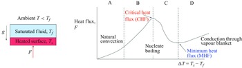


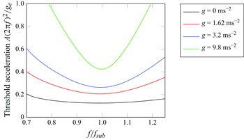


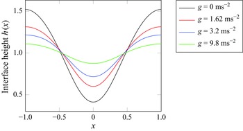


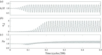


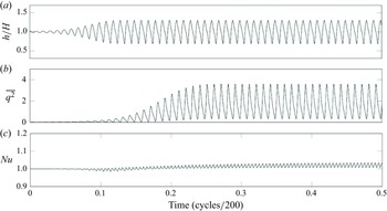


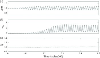


 Open access