


1. Introduction
The classic problem of ship waves has been extensively studied since Lord Kelvin's fascinating discovery in 1887 (Thomson Reference Thomson1887). Kelvin's discovery revealed a constant sector of waves, beyond which stationary ship wakes vanish in an ideal flow over deep water, as depicted in figure 1. A majority of the previous works deal with stationary waves which are seen by a moving observer together with the advancing vessel responsible for the generation of these waves (see, Wehausen Reference Wehausen1973; Reed & Milgram Reference Reed and Milgram2002; Li & Ellingsen Reference Li and Ellingsen2016b; Yuan et al. Reference Yuan, Chen, Jia, Ji and Incecik2021 among others). It has been somewhat taken for granted that investigating stationary ship waves in an Earth-fixed system only involves a transformation of the coordinate system from a moving to an Earth-fixed one. In this work, we revisit the classic problem of ship waves in the ‘eyes’ of an Earth-fixed observer and demonstrate that it is not as trivial as would have been imagined. Instead, we highlight that there are newly emerging needs for a deeper understanding of the underlying physics within an Earth-fixed coordinate system, as explained in detail in the following.

Figure 1. Wave crestlines of the Kelvin wake in the coordinate system moving with the ship composed of transverse waves (blue solid line) and divergent waves (red solid line) confined within the cusp lines (black dashed line) of Kelvin angle  $\gamma _{c}=\arctan (1/\sqrt {8})\approx 19^{\circ }28'$; $\kappa =g/U^2$ where $U$ denotes the ship's speed, and g is the gravitational acceleration.
While the importance of ship waves has been well known in many applied engineering fields because of its relevance to the wave-making resistance of vessels, see, e.g. Yeung (Reference Yeung1972), Beck, Newman & Tuck (Reference Beck, Newman and Tuck1975), Nakos & Sclavounos (Reference Nakos and Sclavounos1990), Noblesse, Huang & Yang (Reference Noblesse, Huang and Yang2013), Li, Smeltzer & Ellingsen (Reference Li, Smeltzer and Ellingsen2019) and He et al. (Reference He, Wu, Yang, Zhu, Li and Noblesse2021), it has been increasingly recognised in the community of coastal morphology and natural hazards in the sea and coastal waters in recent decades. In the semi-sheltered and coastal areas, waves generated by ship transits are a major source of impact on coastal environments (Forlini et al. Reference Forlini, Qayyum, Malej, Lam, Shi, Angelini and Sheremet2021). They can not only erode the bank of the waterway and coastal line, but also pose a potential hazardous impact on coastal structures or berthed floating bodies (Bourne Reference Bourne2000; Soomere Reference Soomere2007; Rapaglia et al. Reference Rapaglia, Zaggia, Parnell, Lorenzetti and Vafeidis2015; Gabel, Lorenz & Stoll Reference Gabel, Lorenz and Stoll2017; Scarpa et al. Reference Scarpa, Zaggia, Manfè, Lorenzetti, Parnell, Soomere, Rapaglia and Molinaroli2019). An advancing vessel can act as a source of propagating wake wash, generating wakes that force sediment transport and drive vertical mixing, which is important to aquatic ecosystems (Rapaglia et al. Reference Rapaglia, Zaggia, Parnell, Lorenzetti and Vafeidis2015; Gabel et al. Reference Gabel, Lorenz and Stoll2017; Meyers et al. Reference Meyers, Luther, Ringuet, Raulerson, Sherwood, Conrad and Basili2021). Thereby, how to quantify the impact of ship wakes on the coastal environments is an open and essential question for coastal management and protection. The answer to this question greatly relies on an in-depth physical understanding of ship wakes measured at fixed locations, which has not been fully available due to limited studies. To this end, this work aims to fill in the knowledge gaps.
There are available methods that have been developed for retrieving the physical properties of ship waves measured at fixed locations. One such, the method of short-time Fourier transform with respect to a record of time series, was pioneered by Wyatt & Hall (Reference Wyatt and Hall1988) and has been widely used in processing wave probe measurements in the last decade (Didenkulova et al. Reference Didenkulova, Sheremet, Torsvik and Soomere2013; Sheremet, Gravois & Tian Reference Sheremet, Gravois and Tian2013; Torsvik et al. Reference Torsvik, Soomere, Didenkulova and Sheremet2015; Pethiyagoda, McCue & Moroney Reference Pethiyagoda, McCue and Moroney2017). Sheremet et al. (Reference Sheremet, Gravois and Tian2013) utilised the short-time Fourier transform to investigate the statistics regarding measured ship wakes, identifying an up-chirping frequency component. Moreover, it has been used in the cases of water of finite depth (Pethiyagoda et al. Reference Pethiyagoda, Moroney, Macfarlane, Binns and McCue2018) and more general cases where the ship advances at a non-constant speed (Pethiyagoda et al. Reference Pethiyagoda, Moroney, Macfarlane and McCue2021).
Compared with other remote sensing techniques, such as satellite photography (Liu, Peng & Chang Reference Liu, Peng and Chang1997; Rabaud & Moisy Reference Rabaud and Moisy2013) and synthetic aperture radar (Lyden et al. Reference Lyden, Hammond, Lyzenga and Shuchman1988; Reed & Milgram Reference Reed and Milgram2002; Karakuş, Rizaev & Achim Reference Karakuş, Rizaev and Achim2020), a distinctive feature of the method is the simplicity at an adequate level of accuracy since it only requires one-point measurement. It can especially lead to the amplitude of waves with different frequencies. This approach relying on one-point measurements particularly facilitates the analysis of wave amplitudes across different frequencies by steadily advancing sailing ships. Torsvik et al. (Reference Torsvik, Soomere, Didenkulova and Sheremet2015) reported that the measured linear waves contain two different components: one with a constant frequency and the other with increasing frequency corresponding to transverse and divergent waves, respectively. They established a correlation between wave frequency, propagation direction, ship speed and distance from the sailing line. The second-order nonlinear ship waves can lead to four extra frequencies, according to Pethiyagoda et al. (Reference Pethiyagoda, McCue and Moroney2017). The time-frequency heat maps are obtained by Buttle et al. (Reference Buttle, Pethiyagoda, Moroney, Winship, Macfarlane, Binns and McCue2022) for waves generated by slender ships, which are validated through comparisons with the experimental findings reported by Buttle et al. (Reference Buttle, Pethiyagoda, Moroney, Winship, Macfarlane, Binns and McCue2020). The same experimental results from waves measured by an array of fixed probes are also used to validate the theory derived from this work.
When a ship passes different physical locations, ring waves are generated at each of the ship locations (Li & Ellingsen Reference Li and Ellingsen2015, Reference Li and Ellingsen2016a). These waves can pass a fixed location with different frequencies as their origins are different due to the time-varying positions of the ship relative to the fixed location which measures the (unsteady) ship waves (see, e.g. Liang, Santo & Si Reference Liang, Santo and Si2022; Liang, Li & Chen Reference Liang, Li and Chen2023). This physical process means the need for more than just measuring the amplitude and frequency of ship waves at a particular location. There are more essential physical properties that are desired, especially the fluid particle velocities and the direction of wave propagation due to passing ship waves. To this end, novel approaches are required to complement the available aforementioned methods. This study will focus on introducing a novel approximate method to address these requirements.
In summary, the objective of this work is threefold. Firstly, we aim to provide a clear explanation of the conditions under which ship waves can pass a fixed location. Secondly, based on these conditions, we derive explicit expressions for various physical properties of these waves, such as amplitude, wave incidence angle, group and phase velocity and fluid particle velocities resulting from passing ship waves. In contrast to the limitations of time–frequency spectrograms, which can only estimate wave amplitude, our analytical expressions enable straightforward estimations of multiple physical quantities. Notably, we demonstrate that the amplitudes of transverse and divergent waves measured at a fixed location can also be expressed using the Kochin function, which is associated with the geometry of the ship hull. Thirdly, leveraging the analytical expressions for physical quantities, we propose a novel method that relies on measurements from two probes fixed at distinct locations to determine the speed and direction of the vessel responsible for generating the observed waves. This approach offers an efficient and accurate means of vessel tracking, allowing for practical applications in maritime management.
The layout of the present paper is as follows. In § 2, waves generated by a ship hull are modelled by a Hogner model (Hogner Reference Hogner1923) in conjunction with the viscous-ship-wave Green function (Liang & Chen Reference Liang and Chen2019). As a sequel to § 2, a uniform Kelvin–Havelock–Peters (KHP) asymptotic approximation (Wu et al. Reference Wu, He, Zhu and Noblesse2018; Liang et al. Reference Liang, Wu, He and Noblesse2020b) is employed in § 3 to explicitly decompose the wave pattern inside the Kelvin wake into transverse and divergent waves. In § 4, physical quantities for both transverse and divergent waves propagating in an Earth-fixed frame of reference are derived, and the long-time asymptotic behaviours are discussed. Building upon the physical properties of transverse and divergent waves, a two-probe method is developed to determine the ship's speed and sailing direction in § 5. The results, particularly the underlying physics, are discussed in § 6. Concluding remarks and future perspectives are presented in § 7.
2. Description of ship waves
In this section, we focus on the description of linear surface waves generated by a steadily advancing object. We employ the viscous-ship-wave Green function, which satisfies the linear free surface boundary condition, to construct the solution as discussed in § 2.2. Additionally, we adopt the Hogner model, as presented in § 2.3, to simulate the free surface flows around the ship hull.
2.1. Statement of the problem
Stationary waves from the perspective of an observer positioned on the ship responsible for the generation of the waves are described. To distinguish these waves from those measured at fixed locations, we consider two frames of reference, as illustrated in figure 2.

Figure 2. Definition of global and local coordinate systems. The global coordinate system  $OXYZ$ is fixed in space, and the sensor is located at $(X,Y)=(0,Y_s)$. The local coordinate system moves steadily with the ship at a constant speed $U$. At $t=0$, the two coordinate systems coincide.
The first frame of reference corresponds to an Earth-fixed Cartesian coordinate system  $OXYZ$, where the $OX$ axis points in the direction of the ship's bow and the $OZ$ axis points upward. In this system, the ship moves at a constant speed $U$ along the positive $OX$ direction. The second coordinate system $oxyz$ moves with the ship, and its origin is fixed at the centre of the ship. Consequently, we establish the relationships $x=X-Ut$, $Y=y$ and $Z=z$, which relate the coordinates in the two frames of reference.
In the moving coordinate system  $oxyz$, the physical problem is steady, and can be defined as a ship hull in the presence of a uniform stream with a velocity $U$ in the direction of the negative $ox$ axis. Then, the velocity potential $\varPhi$ in the flow field is
 \begin{equation} \varPhi(x,y,z)=U[-x+\phi(x,y,z)], \end{equation}
where  $\phi$ denotes the potential disturbed by the presence of ship hull.
The perturbed potential  $\phi$ satisfies the linearised Kelvin–Michell free surface condition with viscous effects (Dias, Dyachenko & Zakharov Reference Dias, Dyachenko and Zakharov2008; Liang & Chen Reference Liang and Chen2019)
 \begin{equation} U^2\frac{\partial^2\phi}{\partial x^2} +g \frac{\partial\phi}{\partial z} + 4\nu_{0} U\frac{\partial^3\phi}{\partial x\partial z^2}=0,\quad \text{at}\ z=0, \end{equation}
where  $\nu _{0}$ denotes the kinematic fluid viscosity coefficient. The combined boundary condition on a still water surface given by (2.2) is based on the weakly damped free surface flow theory, see, e.g. Dias et al. (Reference Dias, Dyachenko and Zakharov2008) for details. The magnitude of the viscous term in this condition is negligibly small compared with the remaining terms (Liang & Chen Reference Liang and Chen2019). This suggests the flow considered is nearly irrotational, thereby the velocity potential in the statement of the (far-field) ship-wave problem is interpreted as a leading-order approximation. The body boundary condition on the hull surface is given by
 \begin{equation} \frac{\partial\phi}{\partial n}=n_{x}, \end{equation}
where the normal vector is defined as positive pointing inwards to the fluid domain. The unknown velocity potential in the viscous boundary condition on a still water surface and the wet surface of the ship hull in calm water given by (2.2) and (2.3), respectively, is solved through a viscous-ship-wave Green function presented in § 2.2 combined with a Hogner model detailed in § 2.3.
2.2. Viscous-ship-wave Green function
The viscous-ship-wave Green function derived by Liang & Chen (Reference Liang and Chen2019) is reviewed in this section, which, taking into account the fluid viscosity, represents the flow induced by a point singularity with unit strength, translating steadily along a straight path in calm water. We remark that such a Green function especially has the feature of removing non-physical behaviours of the classic ship-wave Green function, see, e.g. Ursell (Reference Ursell1960), Clarisse & Newman (Reference Clarisse and Newman1994) and Chen & Wu (Reference Chen and Wu2001). For example, unbounded wave amplitudes in the region near the course of the moving point singularity.
Following Liang & Chen (Reference Liang and Chen2019), the viscous-ship-wave Green function satisfying the free surface condition (2.2) is written as
 \begin{align} 4{\rm \pi} G(\boldsymbol{x},\boldsymbol{\xi})=-{1}/{r}+{1}/{d}+G^{F}, \quad\text{with}\ \left\{ \begin{array}{@{}c@{}} r\\ d \end{array} \right\} =\sqrt{(x-\xi)^2+(y-\eta)^2+(z\mp\zeta)^2}, \end{align}
where  $\boldsymbol {x}\equiv (x,y,z)$ and $\boldsymbol {\xi }\equiv (\xi,\eta,\zeta )$ denote the flow-field point and source point, respectively, and $G^{F}$ is the free surface term in the form of a double Fourier integral. The free surface term $G^{F}=G^{L}+G^{W}$ can be decomposed into a non-oscillatory local-flow component $G^{L}$ and a wave component $G^{W}$ dominant in the far field (see Appendix A for details). The local-flow component $G^{L}$ is
 \begin{equation} G^{L}=\frac{2\kappa}{\rm \pi} \mathrm{Im}\int_{-1}^{1} \mathrm{e}^{Z}E_{1}(Z) \,\mathrm{d} q, \end{equation}
with
 \begin{equation} Z=-\mathrm{i} \kappa\,\sqrt{1-q^2} \left[-|x-\xi| + \mathrm{i} \sqrt{1-q^2} (z+\zeta)-\mathrm{i} q(y-\eta)\right]\!, \end{equation}
and the wave component  $G^{W}$ is
 \begin{equation} G^{W}=-4 H(\xi-x) \mathrm{Im}\int_{-\infty}^{\infty} \kappa {\mathcal{E}}(\boldsymbol{x},q)\tilde{{\mathcal{E}}}(\boldsymbol{\xi},q) \,\mathrm{d} q, \end{equation}
with
 \begin{gather} {\mathcal{E}}(\boldsymbol{x},q)= \exp\left[\kappa(1+q^2)z+4\epsilon \kappa x \frac{(1 + q^2)^3}{1 + 2q^2}-\mathrm{i}\kappa\sqrt{1+q^2}(x +q y)\right]\!, \end{gather}
 \begin{gather} \tilde{{\mathcal{E}}}(\boldsymbol{\xi},q)=\exp\left[\kappa(1+q^2)\zeta-4\epsilon \kappa \xi \frac{(1 + q^2)^3}{1 + 2q^2}+\mathrm{i}\kappa\sqrt{1+q^2}(\xi +q \eta)\right]\!, \end{gather}
where  $\mathrm {e}^{u}E_{1}(u)$ is the complex exponential-integral function (Abramowitz & Stegun Reference Abramowitz and Stegun1964), $\epsilon$ is a parameter associated with viscous effects defined as $\epsilon =g\nu _{0}/U^3$ and $\kappa$ is defined as $\kappa =g/U^2$, which can be interpreted as the wavenumber along the ship's track. In (2.6a), $H(u)$ means the Heaviside step function, which equals to $1$ for $u>0$, or $0$ otherwise.
2.3. Hogner model
The Hogner model due to Hogner (Reference Hogner1923) has been widely used to express the unknown velocity potential,  $\phi$, in an explicit form. It has been tested and proven to be adequate in approximating linear ship waves (Zhang et al. Reference Zhang, He, Zhu, Yang, Li, Zhu, Lin and Noblesse2015; Wu et al. Reference Wu, He, Liang and Noblesse2019; Buttle et al. Reference Buttle, Pethiyagoda, Moroney, Winship, Macfarlane, Binns and McCue2022).
Following Hogner (Reference Hogner1923), the velocity potential due to the flow induced by an advancing ship hull is represented by a source distribution with strength  $n_{\xi }$ over the mean wetted hull surface denoted by $\varSigma ^{H}(\xi,\eta,\zeta )$
 \begin{equation} \phi(\boldsymbol{x})= \iint_{\varSigma^{H}}n_{\xi} G(\boldsymbol{x},\boldsymbol{\xi}) \,\mathrm{d} S, \end{equation}
where  $n_{\xi }$ is the component in the $x$-direction of the vector normal to the ship's hull. Introducing polar coordinates $(x,y)\equiv R(-\cos \gamma,\sin \gamma )$, where $\gamma$ is measured from the negative $x$-axis in the clockwise direction (figure 2), the free surface elevation, denoted by $E(x,y)$, at a location far away from the ship where $R/L\gg 1$, is written in the Fourier–Kochin form given by
 $$\begin{align} E(x,y)&=\frac{1}{\kappa}
\left.\frac{\partial\phi}{\partial x}\right|_{z=0} \approx
\frac{1}{4{\rm \pi}\kappa} \iint_{\varSigma^{H}}n_{\xi}
\left.\frac{\partial
G^{W}(\boldsymbol{x},\boldsymbol{\xi})}{\partial
x}\right|_{z=0} \,\mathrm{d} S\nonumber\\ &=
\frac{\kappa}{\rm \pi} \mathrm{Re}\int_{-\infty}^{\infty}
K(q,x)\exp[{\mathrm{i}\kappa R\psi(q,\gamma)}] \,\mathrm{d}
q,
\end{align}$$
$$\begin{align} E(x,y)&=\frac{1}{\kappa}
\left.\frac{\partial\phi}{\partial x}\right|_{z=0} \approx
\frac{1}{4{\rm \pi}\kappa} \iint_{\varSigma^{H}}n_{\xi}
\left.\frac{\partial
G^{W}(\boldsymbol{x},\boldsymbol{\xi})}{\partial
x}\right|_{z=0} \,\mathrm{d} S\nonumber\\ &=
\frac{\kappa}{\rm \pi} \mathrm{Re}\int_{-\infty}^{\infty}
K(q,x)\exp[{\mathrm{i}\kappa R\psi(q,\gamma)}] \,\mathrm{d}
q,
\end{align}$$
where  $G^W$ is the wave component given by (2.6a). In the wavenumber ( $q$) integral (2.8), $K(q,x)$ is the Kochin function determined by the ship hull geometry written as
 \begin{equation} K(q,x)=\sqrt{1+q^2} \exp\left[4\epsilon \kappa x\frac{(1 + q^2)^3}{1 + 2q^2}\right] \iint_{\varSigma^{H}} n_{\xi}H(\xi-x) \tilde{{\mathcal{E}}}(\boldsymbol{\xi},q) \,\mathrm{d} S, \end{equation}
and the phase function  $\psi (q,\gamma )$ by
 \begin{equation} \psi(q,\gamma)=\sqrt{1+q^2}(\cos\gamma-q \sin\gamma), \end{equation}
consistent with that in (2.6b). The velocity vector due to the ship-motion-induced flow, denoted by  $\boldsymbol {u}=[u^{x},u^{y},u^{z}]^{{\rm T}}$, can be obtained from the velocity potential through
 \begin{align} \boldsymbol{u} \equiv \boldsymbol{\nabla} \phi(\boldsymbol{x}) &= \iint_{\varSigma^{H}}n_{\xi} \boldsymbol{\nabla}_{\boldsymbol{x}}G(\boldsymbol{x},\boldsymbol{\xi}) \,\mathrm{d} S\nonumber\\ & \approx \frac{\kappa^2}{\rm \pi} \mathrm{Re}\int_{-\infty}^{\infty} \left[\begin{array}{c} 1\\ q\\ \mathrm{i}\sqrt{1+q^2} \end{array}\right] K(q,x) \exp({\kappa[(1+q^2)z+\mathrm{i} R\psi(q,\gamma)]}) \,\mathrm{d} q. \end{align}
3. Decomposition of transverse and divergent waves
As is widely known, the stationary ship wake consists of both transverse and divergent waves which have different physical features (Li Reference Li2018; Liang & Chen Reference Liang and Chen2018). Based on the surface elevation given by (2.8), we derive a new approximation to (2.8) in the far field, permitting the explicit partition of ship waves into the transverse and divergent waves. This is achieved through the use of the KHP approximation, whose advantageous features compared with other approximations can be found in other works e.g. Liang et al. (Reference Liang, Wu, He and Noblesse2020b) and Wu et al. (Reference Wu, He, Zhu and Noblesse2018). The application of the asymptotic approximation indicates that the waves in the far field are concerned. This implies that we neglect the effects of ship bow waves, which typically exhibit strong nonlinear behaviour. Nevertheless, the bow waves are confined to the vicinity of the ship, and thus it is sensible to neglect their effects in the far field (Fontaine, Faltinsen & Cointe Reference Fontaine, Faltinsen and Cointe2000).
3.1. Stationary phase points and saddle points
Within the Kelvin wake, characterised by polar angles  $\gamma <\gamma _{c}\equiv 19^{\circ }28'$, there are two distinct stationary phase points requiring the vanishing of the first-order derivative of the phase function, i.e. $\psi '(q,\gamma ) = 0$, where the prime $'$ means differentiation with variable $q$. Then, the stationary phase points are given by
 \begin{equation} q_{{\pm}}=(1\pm Q)\cot\gamma/4, \quad\text{with}\ Q=\sqrt{1-8\tan^2\gamma}, \end{equation}
and the corresponding second-order derivatives are
 \begin{equation} \psi''_{{\pm}}\equiv \frac{\partial^{2}\psi(q_{{\pm}},\gamma)}{\partial q^2} ={\mp}\frac{4}{\sqrt{3}} \frac{Q\sin\gamma}{\sqrt{(1\pm Q)(1\mp Q/3)}}, \end{equation}
where subscripts ‘ $-$’ and ‘ $+$’ correspond to transverse and divergent waves, respectively, hereafter.
At the cusp line of the Kelvin wake  $\gamma =\gamma _{c} =\arctan (1/\sqrt {8})$, two stationary phase points coalesce $q_-=q_+=q_{c}=1/\sqrt {2}$, and both first- and second-order derivatives of the phase function are nil, e.g. $\psi '(q_{c},\gamma _{c}) =\psi ''(q_{c},\gamma _{c})= 0$. The third- and fourth-order derivatives at $q_c$ are
 \begin{equation} \psi'''_{c}\equiv \frac{\partial^{3}\psi(q_{c},\gamma_{c})}{\partial q^{3}} =-4\sqrt{6}/9, \quad\text{and}\quad \psi''''_{c} \equiv\frac{\partial^{4}\psi(q_{c},\gamma_{c})}{\partial q^{4}}=8\sqrt{3}/9. \end{equation}
 Outside the Kelvin wake, when  $\gamma >\gamma _{c}$, the two stationary phase points transform into two complex saddle points, forming a complex conjugate pair. To evaluate the integral, the integration path is deformed, and only the contribution from the saddle point with an imaginary part of $\psi ''$ that is positive matters. The selected saddle point is
 \begin{equation} q_{o}=(1-{\mathcal{Q}})\cot\gamma/4, \quad\text{with}\ {\mathcal{Q}}=\mathrm{i}\sqrt{8\tan^2\gamma-1}, \end{equation}
and the corresponding second-order derivative is
 \begin{equation} \psi''_{o}\equiv \frac{\partial^{2}\psi(q_{o},\gamma)}{\partial q^2}= \frac{4}{\sqrt{3}} \frac{{\mathcal{Q}}\sin\gamma}{\sqrt{(1- {\mathcal{Q}})(1+ {\mathcal{Q}}/3)}}. \end{equation}
3.2. Decomposition via the KHP approximation
The KHP approximation has been extensively studied in Wu et al. (Reference Wu, He, Zhu and Noblesse2018) and Liang et al. (Reference Liang, Wu, He and Noblesse2020b), delving into mathematical derivations and accuracy assessments. However, these works predominantly focus on the mathematical aspects rather than investigating the physical perspective. One notable advantage of the KHP approximation over other counterparts, Chester–Friedman–Ursell (CFU) approximation (Chester, Friedman & Ursell Reference Chester, Friedman and Ursell1957), is its ability to decompose the wave pattern within the Kelvin wedge into transverse and divergent waves, a facet not considered in Wu et al. (Reference Wu, He, Zhu and Noblesse2018) and Liang et al. (Reference Liang, Wu, He and Noblesse2020b). This subsection aims to concentrate specifically on this aspect, elucidating the wave pattern decomposition via the KHP approximation.
Based on Liang et al. (Reference Liang, Wu, He and Noblesse2020b), the KHP approximations to the surface elevation,  $E$, and velocity vector $\boldsymbol {u}=[u^x,u^y,u^z]^{{\rm T}}$ in the flow region inside the cusp of the Kelvin wake $\gamma \le \gamma _{c}$ are expressed as
 $$\begin{align} \left[ \begin{array}{@{}c@{}}
E(x,y) \\ u^x(\boldsymbol{x}) \\ u^y(\boldsymbol{x}) \\
u^z(\boldsymbol{x}) \end{array} \right] &= \left[
\begin{array}{@{}c@{}} E_+(x,y) \\ u^x_+(\boldsymbol{x}) \\
u^y_+(\boldsymbol{x}) \\ u^z_+(\boldsymbol{x}) \end{array}
\right] +\left[ \begin{array}{@{}c@{}} E_-(x,y) \\
u^x_-(\boldsymbol{x}) \\ u^y_-(\boldsymbol{x}) \\
u^z_-(\boldsymbol{x}) \end{array} \right]\nonumber\\
\text{with} \left[ \begin{array}{@{}c@{}} E_{{\pm}}(x,y) \\
u^x_{{\pm}}(\boldsymbol{x}) \\ u^y_{{\pm}}(\boldsymbol{x})
\\ u^z_{{\pm}}(\boldsymbol{x}) \end{array} \right] &=
\mathrm{Re} \left\{ \left[ \begin{array}{@{}c@{}}
{\mathcal{E}}_{{\pm}} \\ {\mathcal{U}}^x_{{\pm}} \\
{\mathcal{U}}^y_{{\pm}} \\ {\mathcal{U}}^z_{{\pm}}
\end{array} \right] \exp[{\mathrm{i} (\kappa R \psi_{{\pm}}
\mp {\rm \pi}/4)}] \right\}\!,
\end{align}$$
$$\begin{align} \left[ \begin{array}{@{}c@{}}
E(x,y) \\ u^x(\boldsymbol{x}) \\ u^y(\boldsymbol{x}) \\
u^z(\boldsymbol{x}) \end{array} \right] &= \left[
\begin{array}{@{}c@{}} E_+(x,y) \\ u^x_+(\boldsymbol{x}) \\
u^y_+(\boldsymbol{x}) \\ u^z_+(\boldsymbol{x}) \end{array}
\right] +\left[ \begin{array}{@{}c@{}} E_-(x,y) \\
u^x_-(\boldsymbol{x}) \\ u^y_-(\boldsymbol{x}) \\
u^z_-(\boldsymbol{x}) \end{array} \right]\nonumber\\
\text{with} \left[ \begin{array}{@{}c@{}} E_{{\pm}}(x,y) \\
u^x_{{\pm}}(\boldsymbol{x}) \\ u^y_{{\pm}}(\boldsymbol{x})
\\ u^z_{{\pm}}(\boldsymbol{x}) \end{array} \right] &=
\mathrm{Re} \left\{ \left[ \begin{array}{@{}c@{}}
{\mathcal{E}}_{{\pm}} \\ {\mathcal{U}}^x_{{\pm}} \\
{\mathcal{U}}^y_{{\pm}} \\ {\mathcal{U}}^z_{{\pm}}
\end{array} \right] \exp[{\mathrm{i} (\kappa R \psi_{{\pm}}
\mp {\rm \pi}/4)}] \right\}\!,
\end{align}$$
where  $\boldsymbol {x}\equiv (x,y,z)$ with the horizontal coordinates further expressed by $(x,y)\equiv R(-\cos \gamma,\sin \gamma )$, and the components $[{\mathcal {E}}_{\pm },{\mathcal {U}}^x_{\pm },{\mathcal {U}}^y_{\pm },{\mathcal {U}}^z_{\pm }]^{\rm T}$ are
 \begin{align} \left[ \begin{array}{@{}c@{}} {\mathcal{E}}_{{\pm}} \\ {\mathcal{U}}^x_{{\pm}} \\ {\mathcal{U}}^y_{{\pm}} \\ {\mathcal{U}}^z_{{\pm}} \end{array} \right] = \frac{\kappa}{\rm \pi} \left[ \frac{\sqrt{2{\rm \pi}}}{\sqrt{\kappa R|\psi''_{{\pm}}|}} (1-\mathrm{e}^{-a^{4/3}}) \boldsymbol{K}(q_\pm,\boldsymbol{x})+ \frac{C_{H}^{*}\mathrm{e}^{-a^{4/3}} }{(\kappa R |\psi'''_c|)^{1/3} } (1\mp \mathscr{F})\boldsymbol{K}(q_c,\boldsymbol{x}) \right], \end{align}
with  $C_{H}^{*}\equiv \varGamma (1/3)/6^{1/6}\approx 1.987334$ and $a=3\kappa R |\psi (q_+)-\psi (q_-)|/4$. In (3.7), the vector function $\boldsymbol {K}$ is defined as
 \begin{equation} \boldsymbol{K}(q,\boldsymbol{x}) \equiv \left[ \begin{array}{@{}c@{}} {\mathcal{K}}^e(q,\boldsymbol{x}) \\ {\mathcal{K}}^x(q,\boldsymbol{x}) \\ {\mathcal{K}}^y(q,\boldsymbol{x})\\ {\mathcal{K}}^z(q,\boldsymbol{x}) \end{array} \right] = \left[ \begin{array}{@{}c@{}} K(q,x) \\ \kappa K(q,x)\,\mathrm{e}^{\kappa(1+{q^2})z} \\ \kappa q \,K(q,x)\,\mathrm{e}^{\kappa(1+{q^2})z}\\ \mathrm{i}\,\kappa\,\sqrt{1+{q^2}}\, K(q,x)\,\mathrm{e}^{\kappa(1+{q^2})z} \end{array} \right], \end{equation}
and  $\mathscr {F}$ is an operator to a function $\chi$ with $\chi ={\mathcal {K}}^e$, ${\mathcal {K}}^x$, ${\mathcal {K}}^y$ or ${\mathcal {K}}^z$, defined as
 \begin{equation} \mathscr{F}(\chi) = \frac{\varGamma(2/3)}{\varGamma(1/3)} \left(\left.\frac{\partial \chi}{\partial q}\right|_{q=q_{c}}-\frac{\psi''''_c}{6\psi'''_c}\chi\right) \left(\frac{6}{\kappa R \psi'''_c}\right)^{1/3}, \end{equation}
where  $\varGamma (u)$ denotes the gamma function (Abramowitz & Stegun Reference Abramowitz and Stegun1964).
Equation (3.6) provides an explicit decomposition of the two systems of waves consisting of transverse waves  $E_-$ and divergent waves $E_+$ as well as their induced velocity vector $\boldsymbol {u}_-$ and $\boldsymbol {u}_+$, respectively. At the cusp line of the Kelvin wake, there is a phase difference ${\rm \pi} /2$ of transverse and divergent waves.
The approximation to wave pattern and velocity components outside the cusp of the Kelvin wake  $\gamma \ge \gamma _{c}$ is written as
 \begin{equation} \left[ \begin{array}{@{}c@{}} E(x,y) \\ u^x(\boldsymbol{x}) \\ u^y(\boldsymbol{x}) \\ u^z(\boldsymbol{x}) \end{array} \right] = \mathrm{Re} \left\{ \left[ \begin{array}{@{}c@{}} {\mathcal{E}}_{o} \\ {\mathcal{U}}^x_{o} \\ {\mathcal{U}}^y_{o} \\ {\mathcal{U}}^z_{o} \end{array} \right] \exp[{\mathrm{i} (\kappa R \psi_{o} + {\rm \pi}/4)}] \right\}\!, \end{equation}
where the components  $[{\mathcal {E}}_{o},{\mathcal {U}}^x_{o},{\mathcal {U}}^y_{o},{\mathcal {U}}^z_{o}]^{\rm T}$ are
 \begin{equation} \left[ \begin{array}{@{}c@{}} {\mathcal{E}}_{o} \\ {\mathcal{U}}^x_{o} \\ {\mathcal{U}}^y_{o} \\ {\mathcal{U}}^z_{o} \end{array} \right] = \frac{\kappa}{\rm \pi} \left[ \frac{\sqrt{2{\rm \pi}}}{\sqrt{\kappa R|\psi''_{o}|}} (1-\mathrm{e}^{-b^{4/3}}) \boldsymbol{K}(q_o,\boldsymbol{x}) + \frac{(1-\mathrm{i})C_{H}^{*}\mathrm{e}^{-b^{4/3}} }{(\kappa R |\psi'''_c|)^{1/3} } (\mathrm{e}^{-2b/3}+\mathrm{i}\mathscr{F})\boldsymbol{K}(q_c,\boldsymbol{x}) \right], \end{equation}
with  $b=3\kappa R |\mathrm {Im}(\psi _{o}'')|/2$.
4. Physical properties of ship waves
In the frame of reference moving with the ship, the physics of ship waves is well understood (Lighthill Reference Lighthill1978). The wave pattern, comprising transverse and divergent waves behind the ship, is stationary, meaning it does not change with time. The phase velocity of stationary waves is observed as zero. In contrast, from the perspective of a fixed observer, ship waves are unsteady and the phase velocity in the direction at right angles to wave crests is to be evaluated. It is typical for the propagation direction of stationary ship waves to differ from the direction of the ship motion (Noblesse et al. Reference Noblesse, He, Zhu, Hong, Zhang, Zhu and Yang2014; Li Reference Li2018). Physically, this implies these stationary waves have different angular frequencies. Therefore, in the Earth-fixed coordinate system, the ship waves are time dependent and particularly short crested, as elaborated in this section. In this section, our focus is placed on deriving the physical properties of propagating transverse and divergent waves, such as wave amplitude, frequency, wave heading, phase velocity and group velocity, based on the asymptotic approximations derived in § 3.
4.1. Physical properties of transverse and divergent waves
In the Earth-fixed coordinate system  $OXYZ$, as in figure 2, the free surface elevation induced by a passing ship is
 \begin{equation} E(X,Y,t)=E_+(X,Y,t)+E_-(X,Y,t), \end{equation}
with  $E_-$ and $E_+$ denoting transverse and divergent waves given by (3.6) written in the form of
 \begin{equation} E_{{\pm}}(X,Y,t)= \lVert{\mathcal{E}}_{{\pm}}\rVert\cos[P_{{\pm}}(X,Y,t)], \end{equation}
where the phase functions  $P_{\pm }(X,Y,t)$ are
 \begin{equation} P_{{\pm}}(X,Y,t)= \kappa \sqrt{1+q_{{\pm}}^2}(Ut-X-q_{{\pm}} Y) \mp {\rm \pi}/4 +{\rm Arg}( {\mathcal{E}}^{{\pm}}), \end{equation}
where  ${\rm Arg}({\mathcal {E}}^{\pm })$ means the argument of the complex function ${\mathcal {E}}^{\pm }$ given by (3.7).
Suppose that the sensor location is at  $(X,|Y|)=(0,Y_{s})$ in the fixed coordinate system, and the coordinates in the moving frame of reference are $(x,|y|)=(-Ut,Y_{s})$. Here, $Y_s$ is larger than $0$, which means the sensor will not be located on the track. Following Pethiyagoda et al. (Reference Pethiyagoda, McCue and Moroney2017), we can define a non-dimensional time
 \begin{equation} \tau \equiv Ut/Y_{s} =-x/|y|. \end{equation}
According to the geometrical relation  $\tan \gamma _{c}=1/\sqrt {8}$, as in figure 1, the observation point is located inside the Kelvin wake when $\tau >\sqrt {8}$, and the cusp line of the Kelvin wake meets the sensor at $\tau =\sqrt {8}$.
Based on the phase function (4.3), we obtain the frequencies of transverse waves  $\omega _-$ and divergent waves $\omega _+$ measured at the sensor location $(X,Y)=(0,Y_s)$
 \begin{equation} \omega_{{\pm}}= \kappa U\sqrt{1+q_{{\pm}}^2} = \frac{\sqrt{2}g}{4U} \sqrt{\tau^2+4\pm\tau\sqrt{\tau^2-8}}, \end{equation}
which are consistent with the results by Pethiyagoda et al. (Reference Pethiyagoda, McCue and Moroney2017) obtained from the geometrical relation of the dispersion relation.
Given the non-dimensional time  $\tau$ defined in (4.4), the stationary phase points $q_{\pm }$ given by (3.1) become
 \begin{equation} q_{{\pm}}=\frac{\tau\pm\sqrt{\tau^2-8}}{4}. \end{equation}
According to the phase function given by (4.3), the wavenumbers in the  $X$- and $Y$-directions are obtained
 \begin{equation} k^X_{{\pm}}= \kappa \sqrt{1+q_{{\pm}}^2} =\kappa \sqrt{\frac{\tau^2+4\pm\tau\sqrt{\tau^2-8}}{8}}, \end{equation}
and
 \begin{equation} k^Y_{{\pm}}= \kappa q_{{\pm}}\sqrt{1+q_{{\pm}}^2} = \kappa\frac{\tau\pm\sqrt{\tau^2-8}}{4} \sqrt{\frac{\tau^2+4\pm \tau\sqrt{\tau^2-8}}{8}}, \end{equation}
where superscripts ‘ $X$’ and ‘ $Y$’ indicate the $X$- and $Y$-directions, respectively, hereafter. Furthermore, we can rewrite the frequencies (4.5) as
 \begin{equation} \omega_\pm= \sqrt{g\sqrt{(k_\pm^X)^2+(k_\pm^Y)^2}} =\sqrt{gk_\pm}, \end{equation}
by using (4.7), and with
 \begin{equation} k_\pm=\sqrt{(k_\pm^X)^2+(k_\pm^Y)^2}, \end{equation}
called the wavenumber modulus. Equation (4.8) indicates that both transverse and divergent waves satisfy the deep water dispersion relation  $\omega ^2=gk$ (Newman Reference Newman1977).
According to (4.7), the heading angles of transverse and divergent waves can be determined
 \begin{equation} \beta_{{\pm}}=\arctan\left(\frac{k_{{\pm}}^{Y}}{k_{{\pm}}^{X}}\right) =\arctan\left(\frac{\tau\pm\sqrt{\tau^2-8}}{4}\right)\!. \end{equation}
Equation (4.10) is consistent with the results by Torsvik et al. (Reference Torsvik, Soomere, Didenkulova and Sheremet2015), which are obtained from the analysis of the dispersion relation.
Given the dispersion relation (4.8), i.e. the relationship between frequency and wavenumbers, the phase velocity vector is obtained
 \begin{align}
\boldsymbol{c}_{{\pm}}&=(c_{{\pm}}^{X},c_{{\pm}}^{Y})
=\frac{\omega_{{\pm}}}{k_{{\pm}}}
\frac{(k_{{\pm}}^{X},k_{{\pm}}^{Y})}{k_\pm} =
\frac{U}{1+q_{{\pm}}^2} (1, q_{{\pm}})\notag\\ &=
\frac{8U}{\tau^2+4\pm\tau\sqrt{\tau^2-8}}
\left(1,\frac{\tau\pm\sqrt{\tau^2-8}}{4}\right)\!,
\end{align}
\begin{align}
\boldsymbol{c}_{{\pm}}&=(c_{{\pm}}^{X},c_{{\pm}}^{Y})
=\frac{\omega_{{\pm}}}{k_{{\pm}}}
\frac{(k_{{\pm}}^{X},k_{{\pm}}^{Y})}{k_\pm} =
\frac{U}{1+q_{{\pm}}^2} (1, q_{{\pm}})\notag\\ &=
\frac{8U}{\tau^2+4\pm\tau\sqrt{\tau^2-8}}
\left(1,\frac{\tau\pm\sqrt{\tau^2-8}}{4}\right)\!,
\end{align}and the group velocity vector according to Lighthill (Reference Lighthill1978) is written as
 \begin{equation} \boldsymbol{v}_{{\pm}}=\left(\frac{\partial\omega_{{\pm}}}{\partial k_{{\pm}}^{X}}, \frac{\partial\omega_{{\pm}}}{\partial k_{{\pm}}^{Y}}\right) = \frac{U}{2(1+q_{{\pm}}^2)} (1, q_{{\pm}}) \equiv \dfrac{\boldsymbol{c}_{{\pm}} }{2}, \end{equation}
by differentiating the dispersion relation (4.8).
Consistent with the deep water wave theory, (4.11) and (4.12) indicate that, in the fixed coordinate system, the phase velocity of both transverse and divergent waves aligns with the direction of the group velocity and is twice the magnitude of the group velocity. These results are consistent with the theory of gravity waves in deep water, further reinforcing the validity of the derived expressions for phase and group velocities in the present study.
It is worth mentioning that (4.5) is consistent with the results determined by the geometrical analysis of the dispersion relation in Pethiyagoda et al. (Reference Pethiyagoda, McCue and Moroney2017). This work has in addition offered an analytical expression for the two components of the wave vectors of the ship waves passing a fixed position, i.e. (4.7a,b). Doing so permits wave directions to be readily resolved, and thereby builds a foundation for the inverse method presented in § 5. Moreover, Torsvik et al. (Reference Torsvik, Soomere, Didenkulova and Sheremet2015) have also derived a geometric relation of the wave dispersion relation, the advancing direction of ship motion and the distance of a fixed location to a ship's sailing line in the Earth-fixed coordinate. How the various frequencies measured at the fixed position are related to the transverse and diverging ship waves was not revealed in Torsvik et al. (Reference Torsvik, Soomere, Didenkulova and Sheremet2015) but has been derived analytically by this work, see, e.g. (4.8).
4.2. Long-time asymptotic expressions
The long-time asymptotic approximations for physical quantities derived in § 4.1 are considered here. The long-time asymptotic expressions for frequencies given by (4.5) are
 \begin{align} \omega_-=g/U+O(\tau^{-2}),\quad \text{and}\quad \omega_+=g\tau/(2U)+O(\tau^{-3})=gt/(2Y_{s})+O(\tau^{-3}). \end{align}
 Figure 3 displays the normalised frequencies due to transverse waves  $\omega _-U/g$ and divergent waves $\omega _+U/g$ at a sensor location as a function of non-dimensional time $\tau =Ut/Y_s$, as determined by (4.5).

Figure 3. Normalised frequencies due to transverse waves  $\omega _-U/g$ and divergent waves $\omega _+U/g$ determined by (4.5) vs non-dimensional time $\tau =Ut/Y_s$.
At  $\tau =2\sqrt {2}$, the time instant when the cusp line of the Kelvin wake intersects the sensor, the frequencies of transverse and divergent waves are identical, with a normalised frequency of $\omega _- U/g=\omega _+ U/g=\sqrt {3/2}$.
With the time marching, the scaled frequency  $\omega _- U/g$ of transverse waves remains nearly constant, as indicated by (4.13a,b). On the other hand, the scaled frequency of divergent waves $\omega _+ U/g$ keeps increasing, in a manner linearly proportional to $\tau$.
When  $\tau$ is large, as in (4.13a,b), we have $\omega _-=g/U$, which indicates that the frequency of transverse waves is independent of time $t$, and inversely proportional to the ship's speed $U$. For divergent waves, however, the frequency is $\omega _+=gt/(2Y_{s})$, linearly proportional to the time $t$ but independent of the ship's speed $U$. These long-time properties offer valuable insights into the dynamics of transverse and divergent waves over time and enable us to better analyse the time–frequency spectrogram, which will be elucidated in § 5.
In the same manner, the long-time asymptotic expressions for wave incidence angles are
 \begin{equation} \tan(\beta_-)=0+O(\tau^{-1}) \quad\text{and}\quad \tan(\beta_+)=\tau/2+O(\tau^{-1}). \end{equation}
 Figure 4 shows the heading angles of transverse and divergent waves at a fixed location varying with the non-dimensional time. When the sensor meets the cusp line of the Kelvin wake at  $\tau =2\sqrt {2}$, denoted by the vertical dashed line, the wave heading angles for transverse and divergent waves are identical, and equal to $\arctan (\sqrt {2}/2) \approx 35.26^{\circ }$, which agrees with the study by Torsvik et al. (Reference Torsvik, Soomere, Didenkulova and Sheremet2015). With the time marching, the incidence angle of transverse waves decreases, while that of divergent waves increases. At large non-dimensional times, the long-time asymptotic expressions in (4.14a,b) apply. Accordingly, the transverse waves eventually propagate along the sailing direction, while the divergent waves propagate perpendicular to the sailing line.

Figure 4. Heading angles of transverse waves  $\beta _-$ and divergent waves $\beta _+$ determined by (4.10) as a function of the non-dimensional time $\tau =Ut/Y_s$.
Then, the long-time asymptotic expressions for phase velocities given by (4.3) are
 \begin{equation} \boldsymbol{c}_-=U(1,1/\tau)+O(\tau^{-2}) \quad\text{and}\quad \boldsymbol{c}_+=U(4/\tau^2,2/\tau)+O(\tau^{-3}), \end{equation}
and those for group velocities given by (4.12) are
 \begin{equation} \boldsymbol{v}_-=U[1/2,1/(2\tau)]+O(\tau^{-2}) \quad\text{and}\quad \boldsymbol{v}_+=U(2/\tau^2,1/\tau)+O(\tau^{-3}). \end{equation}
 Due to the fact that the group velocity is in alignment with the phase velocity, and is half the phase velocity in magnitude, only the phase velocity is discussed here. Figure 5 depicts the phase velocity of transverse and divergent waves, determined by (4.11), with respect to the non-dimensional time  $\tau =Ut/Y_{s}$. Notably, when the cusp line intersects the sensor $\tau =2\sqrt {2}$, the in-line and lateral phase velocity components become identical for both transverse and divergent waves. Specifically, the normalised in-line component of the phase velocity is $2/3$, while the lateral component is $\sqrt {2}/3$.

Figure 5. Phase velocity of transverse waves  $\boldsymbol {c}_-$ and divergent waves $\boldsymbol {c}_+$ determined by (4.11) vs the non-dimensional time $\tau =Ut/Y_s$.
As the time progresses, as shown in (4.15a,b), the in-line phase velocity of transverse waves ( $c_-^{X}$) at the sensor location eventually becomes identical to the ship's translating speed. Meanwhile, the lateral phase velocity ( $c_-^{Y}$) decreases in proportion to the inverse of the non-dimensional time ( $\tau =Ut/Y_s$) for transverse waves. However, for divergent waves, both the longitudinal and lateral phase velocities at the sensor location decrease over time. Specifically, the longitudinal phase velocity of divergent waves ( $c_+^{X}$) decreases with the inverse square of the non-dimensional time, leading to a rapid decay rate, as illustrated in figure 5. This decrease indicates a significant change in the behaviour of divergent waves as time advances.
4.3. Velocity components of the fluid particle
Let the time-dependent velocity component of a fluid particle in the Earth-fixed coordinate system be  $\boldsymbol {U}=(u^{X},u^{Y},u^{Z})$.
By applying the explicit expressions for the velocity components presented in § 3.2 in the moving coordinate system, the velocity components in the Earth-fixed coordinate system, when  $Ut-X<2\sqrt {2}|Y|$, are written as
 \begin{equation} \left[ \begin{array}{@{}c@{}}
u^X \\ u^Y \\ u^Z \end{array} \right] = \mathrm{Re}
\left\langle \left[ \begin{array}{@{}c@{}} {\mathcal{U}}^x_{o} \\
{\mathcal{U}}^y_{o} \\ {\mathcal{U}}^z_{o} \end{array}
\right] \exp\left\{\mathrm{i} \left[\kappa\,
\sqrt{1+q_{o}^2}\, (Ut-X-q_{o}Y)+ {\rm \pi}/4\right]\right\}
\right\rangle.
\end{equation}
\begin{equation} \left[ \begin{array}{@{}c@{}}
u^X \\ u^Y \\ u^Z \end{array} \right] = \mathrm{Re}
\left\langle \left[ \begin{array}{@{}c@{}} {\mathcal{U}}^x_{o} \\
{\mathcal{U}}^y_{o} \\ {\mathcal{U}}^z_{o} \end{array}
\right] \exp\left\{\mathrm{i} \left[\kappa\,
\sqrt{1+q_{o}^2}\, (Ut-X-q_{o}Y)+ {\rm \pi}/4\right]\right\}
\right\rangle.
\end{equation}
As  $Ut-X\ge 2\sqrt {2}|Y|$, the measured location is inside the Kelvin wedge and then the velocity components can be decomposed into components due to transverse and divergent waves
 \begin{equation} \left[ \begin{array}{@{}c@{}}
u^X \\ u^Y \\ u^Z \end{array} \right] = \left[
\begin{array}{@{}c@{}} u_+^X \\ u_+^Y \\ u_+^Z \end{array}
\right] +\left[ \begin{array}{@{}c@{}} u_-^X \\ u_-^Y \\ u_-^Z
\end{array} \right]
\end{equation}
\begin{equation} \left[ \begin{array}{@{}c@{}}
u^X \\ u^Y \\ u^Z \end{array} \right] = \left[
\begin{array}{@{}c@{}} u_+^X \\ u_+^Y \\ u_+^Z \end{array}
\right] +\left[ \begin{array}{@{}c@{}} u_-^X \\ u_-^Y \\ u_-^Z
\end{array} \right]
\end{equation}with
 \begin{equation} \left[ \begin{array}{@{}c@{}}
u_{{\pm}}^X \\ u_{{\pm}}^Y \\ u_{{\pm}}^Z \end{array}
\right] = \mathrm{Re} \left\langle \left[ \begin{array}{@{}c@{}}
{\mathcal{U}}^x_{{\pm}} \\ {\mathcal{U}}^y_{{\pm}} \\
{\mathcal{U}}^z_{{\pm}} \end{array} \right]
\exp\left\{\mathrm{i} \left[\kappa\, \sqrt{1+q_{{\pm}}^2}\,
(Ut-X-q_{{\pm}}Y)\mp {\rm \pi}/4\right]\right\} \right\rangle,
\end{equation}
\begin{equation} \left[ \begin{array}{@{}c@{}}
u_{{\pm}}^X \\ u_{{\pm}}^Y \\ u_{{\pm}}^Z \end{array}
\right] = \mathrm{Re} \left\langle \left[ \begin{array}{@{}c@{}}
{\mathcal{U}}^x_{{\pm}} \\ {\mathcal{U}}^y_{{\pm}} \\
{\mathcal{U}}^z_{{\pm}} \end{array} \right]
\exp\left\{\mathrm{i} \left[\kappa\, \sqrt{1+q_{{\pm}}^2}\,
(Ut-X-q_{{\pm}}Y)\mp {\rm \pi}/4\right]\right\} \right\rangle,
\end{equation}
where vectors  $[{\mathcal {U}}^x_{o} ,{\mathcal {U}}^y_{o},{\mathcal {U}}^z_{o}]^{{\rm T}}$ and $[{\mathcal {U}}^x_{\pm } ,{\mathcal {U}}^y_{\pm },{\mathcal {U}}^z_{\pm }]^{{\rm T}}$ are given by (3.11) and (3.7), respectively, and they are dependent on time $t$.
$t$.
5. The inverse method
Based on the physical properties of the ship wake obtained in § 4, we present in this section an inverse method called the two-probe method for obtaining the moving speed and direction of the sailing ship. In contrast to the synthetic aperture radar image which can produce similar information (Reed & Milgram Reference Reed and Milgram2002; Zilman, Zapolski & Marom Reference Zilman, Zapolski and Marom2014; Karakuş et al. Reference Karakuş, Rizaev and Achim2020), the method presented here is much simpler, because it builds upon the time record of the surface elevation at two fixed locations.
We assume that the surface elevation induced by waves generated by a ship moving at a constant speed has been recorded by two single-point probes located at points A and B, as depicted in figure 6. The distance between A and B is denoted by  $\lambda$, and the angle between the ship's sailing line and the straight line crossing A and B is represented by $\theta$, which is currently unknown and needs to be determined. Let $t_{A}$ and $t_{B}$ be the time instants when the cusp of the ship waves reaches probe A and B, respectively. By definition, we set $T = t_{B}-t_{A}$. At time instants $t_{A}$ and $t_{B}$, the centre of the ship is located at points P and Q, respectively, as indicated in figure 6.

Figure 6. Diagram of the two-probe method for the ship's moving speed and direction. A and B are the locations of two fixed with a distance denoted by  $\lambda$. The sailing direction with respect to the sensor deployment line is $\theta$, which is to be determined. The cusp of the Kelvin wedge meets probes A and B when sailing at locations P and Q, respectively.
By utilising the short-time Fourier transform, one can effectively separate components of different frequencies (Sheremet et al. Reference Sheremet, Gravois and Tian2013; Torsvik et al. Reference Torsvik, Soomere, Didenkulova and Sheremet2015; Pethiyagoda et al. Reference Pethiyagoda, McCue and Moroney2017; Liang et al. Reference Liang, Santo, Shao, Law and Chan2020a; Pethiyagoda et al. Reference Pethiyagoda, Moroney, Macfarlane and McCue2021; Buttle et al. Reference Buttle, Pethiyagoda, Moroney, Winship, Macfarlane, Binns and McCue2022). This allows us to create an amplitude heat map representing the time and frequency variation of the waves. As a result, we can obtain the time-dependent wave frequencies  $\omega _{\pm }^{A}$ and $\omega _{\pm }^{B}$ measured at locations A and B, respectively. Here, the subscripts $-$’ and $+$’ correspond to transverse and divergent waves, respectively. By obtaining the time difference $T$ between the measurements at A and B, as defined earlier, we can proceed to determine the ship's speed denoted by $U$ and its angle of motion relative to the straight line AB.
Based on the long-time asymptotic expression of transverse waves given by (4.13a,b), the ship's speed can be given by
 \begin{equation} U = g/\omega_-^{A,B}\quad \text{when transverse waves are in a steady state}, \end{equation}
due to the fact that the frequency of transverse waves is approximately independent of time according to figure 3.
To determine the sailing angle  $\theta$, we introduce the following geometric relation:
 \begin{equation} |\mathrm{MP}|+UT =|\mathrm{MN}|+|\mathrm{NQ}|. \end{equation}
The difference  $|\mathrm {NQ}|-|\mathrm {MP}|$ can be replaced by
 \begin{equation} |\mathrm{NQ}|-|\mathrm{MP}|=2\sqrt{2} (|\mathrm{BN}|-|\mathrm{AM}|),\quad \text{with}\ |\mathrm{BN}|-|\mathrm{AM}|=\lambda\sin\theta, \end{equation}
where the relation  $\tan \gamma _c=1/\sqrt {8}$ has been used. Then, the geometric relation (5.2) gives rise to the following relation:
 \begin{equation} UT=\lambda\cos\theta+2\sqrt{2} \lambda\sin\theta, \end{equation}
which sets up a relation among  $\lambda$, $UT$ and $\theta$. As a consequence, the angle between the deployment line and sailing line $\theta$ is obtained
 \begin{equation} \theta=\arcsin\left(\frac{UT}{3\lambda}\right)-\gamma_{c}, \end{equation}
which gives  $\theta =0$ for $UT=\lambda$, i.e. the ship track in parallel with the line $|AB|$.
Based on (4.13a,b), the frequency for divergent waves is linearly increasing with time at a slope defined as  $S=g/(2Y_{s})$. The measurement of the slope of the upper branch associated with divergent waves gives $S_{A}=g/(2Y_{s}^{A})$ and $S_{B}=g/(2Y_{s}^{B})$, and then the lateral distances from the sailing line $Y_{s}^{A}$ and $Y_{s}^{B}$ can be obtained. Suppose that the cusp line meets the probes A and B at time instants $t_{A}$ and $t_{B}$, respectively. Then, we have
 \begin{equation} \frac{U(t_{A}-t_{0})}{Y_{s}^{A}} =2\sqrt{2} =\frac{U(t_{B}-t_{0})-\lambda\cos\theta}{Y_{s}^{B}}, \end{equation}
where  $t_{0}$ means the time instant when the midship is in alignment with probe A. Combining with (5.5), we obtain an equation with respect to $\theta$
 \begin{equation} \theta=\arcsin\left[\frac{g}{2\lambda}\left(\frac{1}{S_{B}}-\frac{1}{S_{A}}\right)\right]\!, \end{equation}
which determines the direction of the ship's course.
In summary, using the short-time Fourier transform in the two-point measurement method allows us to extract the relevant wave frequencies at locations A and B. This information, combined with the time difference  $T$, enables us to determine the ship's velocity and its sailing direction with respect to the line AB. The two-point measurement method provides a simple but reliable and practical approach for estimating essential navigation parameters based on wave measurements at two distinct locations.
6. Results and discussions
For illustrative purposes, wave patterns generated by a parabolic Wigley hull model are considered, and the geometry of the Wigley hull is defined as
 \begin{equation} y={\pm}\frac{L}{20}\left[1-(2x/L)^2\right] \left[1-(15z/L)^2\right]\!, \end{equation}
which is applied in Buttle et al. (Reference Buttle, Pethiyagoda, Moroney, Winship, Macfarlane, Binns and McCue2022). In (6.1),  $L$ denotes the length of the Wigley hull, and the Froude number associated with the ship's speed is defined as $F=U/\sqrt {gL}$. It is noted that this model is applicable to ships of arbitrary geometry. This is made possible by utilising the Kochin function (2.9), which is directly linked to the wetted surface of the ship's hull. The application of the Hogner model for describing waves generated by a realistic ship hull can be found in Zhang et al. (Reference Zhang, He, Zhu, Yang, Li, Zhu, Lin and Noblesse2015) and Wu et al. (Reference Wu, He, Liang and Noblesse2019).
6.1. Comparison with experiments and verification of the numerical model
We compare the results obtained from the numerical computation of the wavenumber integral (2.8) with experimental measurements reported in Buttle et al. (Reference Buttle, Pethiyagoda, Moroney, Winship, Macfarlane, Binns and McCue2020). Figure 7 illustrates the time history of waves generated by a translating Wigley hull, as described in (6.1), at two distinct sensor locations. The lateral distances from the sailing line to the sensors are  $Y_s=2L$ (a) and $Y_s=3L$ (b), respectively, and the Froude number is $F=0.3259$. Despite the presence of noise in the experimental data, the agreement at both sensor locations is satisfactory, indicating the validity of the present numerical model. The good agreement between the numerical results and experimental measurements further indicates the reliability of the numerical model in capturing the wave patterns induced by a translating ship hull at sensor locations.

Figure 7. Time signal of the free surface elevation created by a Wigley hull at a forward speed  $F=0.3259$. Panels (a,b) correspond to the measurements at $Y_s=2L$ and $Y_{s}=3L$, respectively, from the sailing line. Comparison is made with the experiments reported in Buttle et al. (Reference Buttle, Pethiyagoda, Moroney, Winship, Macfarlane, Binns and McCue2020). Experiments: red solid line, numerical: blue dashed line.
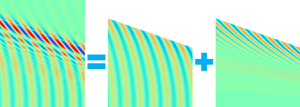
To examine the accuracy of the KHP approximation elucidated in § 3, figure 8 exhibits the coloured plots of wave pattern created by a translating Wigley hull within the rectangular region  $-30\le x/L \le -20$, $0\le y/L\le 12$ at a Froude number $F=0.5$. The free surface elevation is normalised with respect to ship's length ( $E/L$). Results determined by direct numerical integration, CFU approximation (Chester et al. Reference Chester, Friedman and Ursell1957) and KHP approximation (Wu et al. Reference Wu, He, Zhu and Noblesse2018; Liang et al. Reference Liang, Wu, He and Noblesse2020b) are displayed in panels (a,b,c), respectively. It is evident from the plots that there is no significant difference among the three panels, indicating that the KHP approximation accurately approximates the wavenumber integral (2.8).

Figure 8. Wave patterns ( $E/L$) generated by a translating Wigley hull at a Froude number $F=0.5$ determined by direct numerical computation (a), CFU approximation (b) and KHP approximation (c).
In figure 9, the induced velocity components  $\boldsymbol {U}=(u^{X},u^{Y},u^{Z})$ measured at an Earth-fixed location $(X,Y,Z)/L=(0,5,0)$ are presented as a function of non-dimensional time $\tau$ for the Froude number $F=0.5$. The velocity components are non-dimensionalised with respect to the translating speed $U$. Comparison is made between the direction numerical integration of the wavenumber integral and the corresponding KHP approximation, and good agreement between the two methods is obtained.

Figure 9. Non-dimensional induced velocity components  $(u^{X},u^{Y},u^{Z})/U$ measured at the Earth-fixed location $(X,Y,Z)/L=(0,5,0)$ varying with the non-dimensional time $\tau$ for $F=0.5$. Comparison is made between the direction numerical integration (blue solid line) and the KHP approximation (red dotted line).
The good agreement observed in figures 8 and 9 confirms the reliability of the KHP approximation for accurately predicting both the wave pattern and fluid particle velocities induced by a translating ship hull.
6.2. Decomposition into transverse and divergent waves
Figures 10, 11 and 12 exhibit coloured contour plots of wave patterns generated by the Wigley hull at Froude numbers  $F=0.2$, $0.5$ and $0.7$, respectively. The selected Froude numbers are associated with low-speed, medium-speed and high-speed vessels, respectively (Faltinsen Reference Faltinsen2005). The free surface elevation is normalised with respect to ship's length ( $E/L$). Wave patterns, together with their decomposition into transverse and divergent waves inside the Kelvin wedge, are displayed in panels (a,b,c), respectively. The white dashed line in panel (a) corresponds to the cusp line of the Kelvin wake.

Figure 10. Wave patterns (a) as well as decomposition into transverse waves (b) and divergent waves (c) generated by a translating Wigley hull defined in (6.1) at a Froude number  $F=0.2$.

Figure 11. Same as figure 10, but  $F=0.5$.

Figure 12. Same as figure 10, but  $F=0.7$.
At  $F=0.2$, the amplitude of transverse waves is appreciably larger than that of divergent waves, whereas the tendency is reversed at $F=0.7$. The amplitudes of the two wave systems are comparable at $F=0.5$. Therefore, divergent waves play an increasingly dominant role with increasing ship velocity, consistent with the conclusion that divergent waves are dominant for high-speed vessels (Faltinsen Reference Faltinsen2005; Darmon, Benzaquen & Raphaël Reference Darmon, Benzaquen and Raphaël2014). In the panels (b,c), where transverse and divergent waves are displayed, respectively, the profiles are consistent with the iso-phase lines plotted in figure 1, and the wave crests are appreciably deflected near the cusp. In panel (a), wave patterns exhibit short-crested features as a consequence of superposition of transverse and divergent waves.
In figures 10–12, it is observed from the right panels that divergent waves vanish near the ship's track. This is because divergent waves near the track are associated with large wavenumbers, resulting in very short wavelengths according to the asymptotic analysis (Chen Reference Chen2004; Liang & Chen Reference Liang and Chen2018). Consequently, these short waves are significantly damped out under the influence of fluid viscosity effects (Liang & Chen Reference Liang and Chen2019). This observation explains the disappearance of divergent waves near the ship's track in the presented figures.

Figure 13. Time history of the ship wake  $E$ in panel (a) and the decomposition into transverse waves $E_-$ (blue solid line) and divergent waves $E_+$ (red solid line) when $\tau \ge 2\sqrt {2}$ in panel (b). The corresponding amplitude functions $\lVert E_-\rVert$ and $\lVert E_+\rVert$ are plotted by dashed lines. The signal is measured at $(X,Y)=(0,5L)$, and the Froude number is $F=0.2$.
6.3. Time responses at a fixed sensor location
Figures 13, 14 and 15 depict the time histories of the ship wake measured at a fixed sensor location  $(X,Y)=(0,5L)$ for Froude numbers $F=0.2$, $0.5$ and $0.7$, respectively. In panel (a) in each figure, the total signal $E$ is displayed. When $\tau >2\sqrt {2}$, the signal is further decomposed into transverse waves $E_-$ and divergent waves $E_+$, which are shown in panel (b) in each figure. Additionally, the corresponding amplitude functions (envelopes) $\lVert {\mathcal {E}}_-\rVert$ and $\lVert {\mathcal {E}}_+\rVert$, are plotted in panel (b) of each figure as dashed lines.

Figure 14. Same as figure 13, but  $F=0.5$.

Figure 15. Same as figure 13, but  $F=0.7$.
In the vicinity of the time instant  $\tau =2\sqrt {2}$, when the cusp line intersects the sensor, divergent waves play an increasingly significant role with higher ship speeds (larger Froude numbers). With time marching, the frequency of divergent waves increases steadily, as depicted in figure 3. However, despite this increase, divergent waves eventually decay to zero. At the sensor location, the lateral distance from the ship's sailing line remains constant, while the in-line distance consistently increases, resulting in a decreasing polar angle $\gamma$. As explained in Liang & Chen (Reference Liang and Chen2019), divergent waves experience considerable damping for small polar angles due to the influence of fluid viscosity effects. Consequently, the sensor can only measure divergent waves over a finite period of time. By comparing figures 13–15, we observe that the duration of divergent waves increases with the ship's speed. Consequently, the divergent waves generated by a high-speed ship may lead to highly transient responses of near-shore floating structures, which should be taken into account for engineering and safety considerations.
In contrast to divergent waves, the frequency of transverse waves remains nearly constant with time, and their wave amplitude decreases slowly, as depicted by the blue dashed line. Therefore, the influence of transverse waves at the sensor location will persist for an extended period. In panel (b) of the figures, it is observed that the envelope of divergent waves (red dashed line) undergoes modulation, leading to vanishing amplitude at certain locations. These locations correspond to the low-intensity regions in the divergent wave branch of time–frequency spectrograms, which are evident in both numerical simulations and experimental measurements (Pethiyagoda et al. Reference Pethiyagoda, Moroney, Macfarlane, Binns and McCue2018; Buttle et al. Reference Buttle, Pethiyagoda, Moroney, Winship, Macfarlane, Binns and McCue2022). This modulation phenomenon contributes to the intermittent presence of divergent waves, causing variations in their amplitudes over time.
To explore the occurrence of vanishing amplitude in divergent waves at the probed location, we present two sets of plots. In panel (a), we show the time variation of the stationary phase points  $q_{\pm }$ and the corresponding modulus of the Kochin functions $\lVert K_{\pm }\rVert$. Simultaneously, in panel (b), we present the time–frequency spectrograms obtained from the short-time Fourier transform using the scipy library in Python.
Figures 16, 17 and 18 correspond to Froude numbers  $F=0.2$, $0.5$ and $0.7$, respectively. When $\tau >2\sqrt {2}$, the sensor is located within Kelvin's wedge, giving rise to the presence of two distinct stationary phase points, $q_-$ and $q_+$, associated with transverse and divergent waves, respectively, as described in (3.1).

Figure 16. Stationary phase points  $q_{\pm }$ defined by (3.1) and the corresponding Kochin functions $\lVert K_{\pm }\rVert$ in panel (a) and the time–frequency spectrogram obtained from the short-time Fourier transform in panel (b) at $F=0.2$. The physical quantities associated with transverse waves are plotted by solid lines (——), and those with divergent waves are by dashed lines (- - - -). The cyan full circles ( $\bullet$, cyan) denote the locations where the amplitude of divergent waves is diminishing.

Figure 17. Same as figure 16, but  $F=0.5$.

Figure 18. Same as figure 16, but  $F=0.7$.
With the progression of time, the stationary phase point  $q_-$ gradually approaches zero, resulting in a mild variation of the Kochin function for transverse waves, $\lVert K_-\rVert$ with $K_{\pm }=K(q_{\pm },-Ut)$ given by (2.9). In contrast, the stationary phase point $q_+$ continues to increase with time. As a consequence, the corresponding Kochin function $\lVert K_+\rVert$ undergoes modulation, leading to the occurrence of vanishing amplitude in divergent waves.
These locations, where the amplitude of divergent waves disappears, are denoted by cyan full circles, and they cause a discontinuity in the upper branch of the time–frequency spectrograms. This phenomenon provides insight into the intermittent presence of divergent waves and the patterns of amplitude variation in the vicinity of the sensor location.
6.4. Velocity components of the fluid particle
We now focus on examining the velocity components of fluid particles, measured at an Earth-fixed location  $(X, Y, Z)/L = (0, 5, 0)$, induced by ship waves as a function of the non-dimensional time $\tau = Ut/Y$. These velocity components are normalised with respect to the ship's speed $U$. The results corresponding to Froude numbers $F = 0.2$, $0.5$ and $0.7$ are depicted in figures 19, 20 and 21, respectively. Within each figure, the velocity components $u^X$, $u^Y$ and $u^Z$ are respectively exhibited in panels (a), (b) and (c).

Figure 19. Time series of non-dimensional induced velocity components  $(u^{X},u^{Y},u^{Z})/U$ and their decomposition into the components due to transverse waves (blue solid line) and divergent waves (red dashed line). The velocity components are measured at an Earth-fixed location $(X,Y,Z)/L=(0,5,0)$ for the Froude number $F=0.2$.

Figure 20. Same as figure 19, but  $F=0.5$.

Figure 21. Same as figure 19, but  $F=0.7$.
The directional characteristics of transverse and divergent waves, as depicted in figure 4, reveal that transverse waves eventually propagate towards the ship's sailing direction, while divergent waves exhibit an increasing angle until they approach perpendicularity to the ship's course.
At a low Froude number  $F = 0.2$, as in figure 19, the wave pattern predominantly comprises transverse waves that propagate in alignment with the ship's sailing path. Consequently, the velocity field is primarily influenced by components $u^X$ and $u^Z$, while the lateral velocity component $u^Y$, mainly contributed by divergent waves, remains negligible. Upon reaching a Froude number of $F = 0.5$, as in figure 20, the significances of transverse and divergent waves become comparable, resulting in all three velocity components displaying comparable magnitudes. At a higher Froude number $F = 0.7$, as in figure 21), despite the existence of divergent waves within a finite period, their dominant influence is elucidated in § 6.2. Consequently, the velocity field is predominantly influenced by components $u^Y$ and $u^Z$, while the in-line velocity component $u^X$, mainly attributed to transverse waves, becomes inconsequential.
6.5. Showcase of the two-probe method
To demonstrate the effectiveness of the two-point measurement method elucidated in § 5, we devise a problem with a ship model of length  $L=1$ m sailing at a speed $U=1.6\ {\rm m}\ {\rm s}^{-1}$. Two wave probes A and B are at a distance $\lambda =2$ m, and the sailing direction with respect to the deployment line is $\theta =30^{\circ }$.
Figures 22 and 23 exhibit the time histories and the corresponding time–frequency spectrograms obtained from the measurements at probes A and B, respectively. By analysing the frequency of the lower branch of the spectrogram heat map, we determine the frequency of transverse waves as  $\omega _-\approx 6.1\ {\rm rad}\ {\rm s}^{-1}$. Consequently, using (5.1), we compute the corresponding velocity $U_{cal}\approx 1.61\ {\rm m}\ {\rm s}^{-1}$, which is in close agreement with the true value of $1.6\ {\rm m}\ {\rm s}^{-1}$.

Figure 22. Free surface elevation measured at probe A (a), and the corresponding time–frequency spectrogram (b). Grey dashed lines in panel (b) correspond to asymptotic expressions (4.13a,b) for transverse and divergent waves.

Figure 23. Same as figure 22, but at probe B.
By measuring the upper branch associated with divergent waves, we can obtain the slopes  $S_{A}=g/(2Y_{s}^{A})\approx 1.6$ and $S_{B}=g/(2Y_{s}^{B})\approx 1.2$ of frequencies for divergent waves measured at probes A and B. Then, using the relation (5.7), we compute the sailing angle as $\theta _{cal}\approx 30.7^{\circ }$, which shows good agreement with the true value $\theta _{true}=30^{\circ }$. The successful estimation of both the ship's speed and sailing angle through measurements of two branches in the heat map of the time–frequency spectrograms validates the effectiveness of the developed two-point method.
In conclusion, the two-probe method presented here provides a simple but reliable means to estimate the ship's speed and sailing angle by analysing two branches in the time–frequency spectrogram heat map. This method offers a practical solution for obtaining essential navigation information from wave measurements at two distinct locations, proving its potential for real-world applications.
7. Conclusions
This paper investigates the waves observed at fixed locations caused by the passage of a vessel moving at a constant speed. The study derives the physical properties of these waves, which have significant implications for coastal management and protection in the context of climate change and sea-level rise. By employing a combination of the Hogner model and the viscous-ship-wave Green function, we find that the waves are unsteady and exhibit short-crested features, despite the vessel's steady advancement.
The numerical model's validity has been confirmed through comparisons with experimental measurements, demonstrating good agreement. A uniform KHP approximation is used to represent the far-field waves generated by the ship and for the decomposition of the transverse and divergent waves. The physical properties of the transverse and divergent waves are explicitly obtained, including the amplitude, frequency, wavenumber, wave direction, phase velocity and group velocity.
We find that the physical properties of transverse and divergent waves measured at a fixed location can be summarised as follows.
(i) The frequency of transverse waves remains almost constant over time but is inversely proportional to the ship's speed. The frequency of divergent waves is independent of the ship's speed but increases linearly with time.
(ii) Both transverse and divergent waves exhibit that group velocities propagate in the same direction as the phase velocity. The magnitude of the group velocity is half that of the phase velocity, consistent with deep water wave theory.
(iii) When the sensor encounters the cusp line of the Kelvin wake, the heading angles for transverse and divergent waves are identical, both measuring $35.26^{\circ }$. However, as time progresses, the wave propagation angle changes. Specifically, transverse waves will propagate in the direction of the ship's sailing, while divergent waves will propagate towards perpendicularity to the ship's sailing line. Therefore, the induced velocity component aligned with the ship's course is primarily influenced by transverse waves, while the lateral velocity component is dominated by divergent waves.
(iv) A sensor fixed at a particular location can only measure divergent waves for a finite period, with the duration increasing as the ship's speed rises. On the other hand, transverse waves persist for an extended time and decay slowly with the passage of time.

The present study is focused on ship waves in deep water, which can be readily extended to more general cases, e.g. a finite water depth (Yang, Faltinsen & Zhao Reference Yang, Faltinsen and Zhao2006; Zhu et al. Reference Zhu, He, Zhang, Wu, Wan, Zhu and Noblesse2015), ship waves in a background current (Ellingsen Reference Ellingsen2014; Li & Ellingsen Reference Li and Ellingsen2016b), ship waves in the ambient ocean waves (Noblesse & Hendrix Reference Noblesse and Hendrix1992; Chen Reference Chen2004), etc. That being said, the main results obtained from this work are limited to linear and asymptotic waves sufficiently far away from the ship.
Acknowledgements
H.L. warmly thanks Dr R. Pethiyagoda for providing raw data of experiments.
Funding
This work is supported by A*STAR under its RIE 2020 Industry Alignment Fund, grant no. A19F1a0104 (ENSURE), and the National Research Foundation, Singapore and Singapore Maritime Institute under the Maritime Transformation Programme White Space Fund (Centre of Excellence for Autonomous and Remotely Operated Vessels (CEAOPS), Project ID SMI-2019-MTP-01). Y. Li acknowledges the support from the research council of Norway through the Fripro mobility grant (project no. 287389) and the POS-ERC project 342480.
Declaration of interests
The authors report no conflict of interest.
Appendix A. Decomposition of the free surface term
In this appendix, the decomposition of the free surface term  $G^{F}$ into the local-flow and far-field wave components is considered. For convenience, physical variables are non-dimensionalised with respect to the translating speed $U$ and gravitational acceleration $g$
$g$
 \begin{equation} (\tilde{x},\tilde{y},\tilde{z})=\kappa(x-\xi,y-\eta, z+\zeta), \quad {\mathcal{G}}^F=G^F/\kappa, \end{equation}
and then, the free surface term in the form of the double Fourier integral is expressed as (Liang & Chen Reference Liang and Chen2019)
 \begin{equation} {\mathcal{G}}^F=\frac{2}{\rm \pi} \mathrm{Re}\int_{-\infty}^{\infty} \int_{0}^{\infty} \frac{\exp({\tilde{z}\sqrt{\alpha^2+\beta^2}-\mathrm{i}(\alpha \tilde{x}+\beta \tilde{y})})}{\alpha^2-\sqrt{\alpha^2+\beta^2}-4\mathrm{i}\epsilon\alpha(\alpha^2+\beta^2)} \,\mathrm{d}\alpha\,\mathrm{d}\beta. \end{equation}
 The decomposition is realised by means of the Cauchy residue theorem. Equivalent but different from the analysis (Chen Reference Chen2023) based on the polar coordinates  $(k,\theta )$ with $(\alpha,\beta )=k(\cos \theta,\sin \theta )$ for the general case of the ship-motion Green function, here, we perform directly in $(\alpha,\beta )$ plan and take the $\alpha$-integral as the inner integral. The root to the complex dispersion relation in the denominator of (A2) is (Lu & Chwang Reference Lu and Chwang2007)
 \begin{equation} \alpha(\beta)\approx a_0 + \mathrm{i} \epsilon a_1, \end{equation}
where
 \begin{equation} a_0=\sqrt{\frac{1+m}{2}}, \quad\text{and}\quad a_{1}=\frac{(1+m)^3}{2m}, \quad \text{with}\ m=\sqrt{1+4\beta^2}. \end{equation}
 The wave component dominant in the far field is associated with the residue of the  $\alpha$-integral, and it is written in the form of a wavenumber integral (Liang & Chen Reference Liang and Chen2019)
 \begin{align} {\mathcal{G}}^{W}=-4 H(-\tilde{x}) \mathrm{Im}\int_{-\infty}^{\infty} \exp\left[(1+q^2)\tilde{z}+4\epsilon \tilde{x} \frac{(1 + q^2)^3}{1 + 2q^2}-\mathrm{i}\sqrt{1+q^2}(\tilde{x} +q \tilde{y})\right] \,\mathrm{d} q. \end{align}
 Then, we are focused on the simplification of the local-flow component  ${\mathcal {G}}^{L}$, which is missing in Liang & Chen (Reference Liang and Chen2019). Following Noblesse (Reference Noblesse1977), we simplify the integral with respect to $\alpha$, and the corresponding $\alpha$-integral is illustrated in figure 24. We may construct a closed contour including the integration path, a quarter circle with a radius $R\rightarrow \infty$ and a path along the imaginary axis. It can be verified that the integral along the quarter circle vanishes as the radius $R$ tends to infinity. As for the selection of the path along the imaginary axis, it depends on the location of the flow field point upstream or downstream.

Figure 24. Integration contour in the complex  $\alpha -$plane for $\tilde {x}<0$ (a) and $\tilde {x}\ge 0$ (b).
A.1. The case $\tilde {x} < 0$

When  $\tilde {x} < 0$, i.e. downstream, the integration path is deformed to the imaginary axis integrating from $0$ to $\mathrm {i} \infty$, as illustrated in figure 24(a), and the local-flow component in this case is expressed as
 \begin{equation} {\mathcal{G}}^{L} = \frac{2}{\rm \pi} \mathrm{Re} \int_{-\infty}^{\infty} \int_{0}^{\mathrm{i}\infty} \frac{\exp({\tilde{z}\sqrt{\alpha^2+\beta^2} -\mathrm{i} (\alpha\tilde{x}+\beta\tilde{y})})} {\alpha^2-\sqrt{\alpha^2+\beta^2}-4\mathrm{i}\epsilon\alpha(\alpha^2+\beta^2)} \,\mathrm{d} \alpha \,\mathrm{d} \beta. \end{equation}
Introducing  $\alpha = \mathrm {i} t$, (A5) is rewritten as
 \begin{equation} {\mathcal{G}}^{L} = {\mathcal{G}}^{L}_{1} +{\mathcal{G}}^{L}_{2}, \end{equation}
where  ${\mathcal {G}}^{L}_{1}$ and ${\mathcal {G}}^{L}_{2}$ are written as
 \begin{gather} {\mathcal{G}}^{L}_{1} = \frac{2}{\rm \pi} \mathrm{Re} \int_{-\infty}^{\infty} \int_{0}^{\left|\beta\right|} \frac{\mathrm{i}\exp({\tilde{z}\sqrt{\beta^2- t^2} -\mathrm{i} (\mathrm{i} t\tilde{x}+\beta\tilde{y})})} {-t^2-\sqrt{\beta^2- t^2}+4\epsilon t(\beta^2-t^2)} \,\mathrm{d} t\,\mathrm{d} \beta, \end{gather}
 \begin{gather} {\mathcal{G}}^{L}_{2} = \frac{2}{\rm \pi} \mathrm{Re} \int_{-\infty}^{\infty} \int_{\left|\beta\right|}^{\infty} \frac{\mathrm{i}\exp({\mathrm{i} \tilde{z}\sqrt{t^2-\beta^2} -\mathrm{i} (\mathrm{i} t\tilde{x}+\beta\tilde{y})})}{-t^2-\mathrm{i}\sqrt{t^2-\beta^2}+4\epsilon t(t^2-\beta^2)} \,\mathrm{d} t \,\mathrm{d} \beta. \end{gather}
The integrand of  ${\mathcal {G}}^{L}_{1}$ is an odd function with respect to $\beta$, and thus the component ${\mathcal {G}}^{L}_{1}$ is nil. By performing the variable of change $a=\sqrt {t^2-\beta ^2}$, the representation of ${\mathcal {G}}^L$ is
 \begin{equation} {\mathcal{G}}^{L} = \frac{2}{\rm \pi} \mathrm{Re} \int_{-\infty}^{\infty} \int_{0}^{\infty} \frac{\mathrm{i} a\exp({\mathrm{i} a \tilde{z} -\mathrm{i} (\mathrm{i} \tilde{x} \sqrt{a^2+\beta^2}+\tilde{y}\beta)})} {[-(a^2+\beta^2)-\mathrm{i} a+4\epsilon a^2\sqrt{a^2+\beta^2}] \sqrt{a^2+\beta^2}} \,\mathrm{d} a \,\mathrm{d} \beta. \end{equation}
Converting the Cartesian coordinates  $(a,\beta )$ to polar coordinates via introducing $a = \varrho \cos \theta$ and $\beta = \varrho \sin \theta$, (A7) becomes
 $$\begin{gather} {\mathcal{G}}^{L} = \frac{2}{\rm \pi} \mathrm{Re} \int_{-{\rm \pi}/2}^{{\rm \pi}/2} \int_{0}^{\infty} \frac{\mathrm{i} \cos \theta}{\sqrt{1+16\mathrm{i} \epsilon^2\cos^3\theta}} \left(\frac{1}{\varrho-\varrho_+}-\frac{1}{\varrho-\varrho_-}\right)\nonumber\\ \times \exp({\varrho (\tilde{x} + \mathrm{i} \tilde{z} \cos \theta -\mathrm{i} \tilde{y} \sin \theta)}) \,\mathrm{d} \varrho \,\mathrm{d} \theta, \end{gather}$$
where  $\varrho _+$ and $\varrho _-$ are defined as
 \begin{equation} \varrho_+= \frac{1+\sqrt{1+16\mathrm{i}\epsilon\cos^3\theta}}{8\epsilon\cos^2\theta} \approx \frac{1+4\mathrm{i}\epsilon\cos^3\theta}{4\epsilon\cos^2\theta}, \end{equation}
and
 \begin{equation} \varrho_-= \frac{1-\sqrt{1+16\mathrm{i}\epsilon\cos^3\theta}}{8\epsilon\cos^2\theta} \approx-\mathrm{i}\cos\theta. \end{equation}
Using the relation in appendix C in Liang & Chen (Reference Liang and Chen2019), the double integral in (A2) reduces to a single integral
 \begin{equation} {\mathcal{G}}^{L} = \frac{2}{\rm \pi} \mathrm{Re} \int_{-{\rm \pi}/2}^{{\rm \pi}/2} \frac{\mathrm{i} \cos \theta}{\sqrt{1+16\mathrm{i} \epsilon^2\cos^3\theta}} \left[\mathrm{e}^{Z_+}E_{1}(Z_+)-\mathrm{e}^{Z_-}E_{1}(Z_-)\right] \,\mathrm{d} \theta, \end{equation}
where  $\mathrm {e}^{u}E_{1}(u)$ denotes the exponential-integral function, and $Z_{\pm }$ are defined as
 \begin{equation} Z_{{\pm}}= \varrho_{{\pm}} (\tilde{x} + \mathrm{i} \tilde{z} \cos \theta -\mathrm{i} \tilde{y} \sin \theta). \end{equation}
A.2. The case $\tilde {x} \ge 0$

Similar as the deformation of the contour integration performed in (A5), the integration path is deformed to the negative imaginary axis when  $\tilde {x} \ge 0$, as illustrated in figure 24(b), and the corresponding local-flow component is
 \begin{equation} {\mathcal{G}}^{L} = \frac{2}{\rm \pi} \mathrm{Re} \int_{-\infty}^{\infty} \int_{0}^{-\mathrm{i}\infty} \frac{\exp({\tilde{z}\sqrt{\alpha^2+\beta^2} -\mathrm{i} (\alpha\tilde{x}+\beta\tilde{y})})} {\alpha^2-\sqrt{\alpha^2+\beta^2}-4\mathrm{i}\epsilon\alpha(\alpha^2+\beta^2)} \,\mathrm{d} \alpha \,\mathrm{d} \beta. \end{equation}
Introducing  $\alpha = -\mathrm {i} t$, (A10) is rewritten as
 \begin{equation} {\mathcal{G}}^{L} = {\mathcal{G}}^{L}_{1} + {\mathcal{G}}^{L}_{2}, \end{equation}
where
 \begin{gather} {\mathcal{G}}^{L}_{1} = \frac{2}{\rm \pi} \mathrm{Re} \int_{-\infty}^{\infty} \int_{0}^{\left|\beta\right|} \frac{-\mathrm{i}\exp({\tilde{z}\sqrt{\beta^2- t^2} -\mathrm{i} (-\mathrm{i} t\tilde{x}+\beta\tilde{y})})} {-t^2-\sqrt{\beta^2- t^2}-4\epsilon t(\beta^2-t^2)} \,\mathrm{d} t \,\mathrm{d} \beta, \end{gather}
 \begin{gather} {\mathcal{G}}^{L}_{2} = \frac{2}{\rm \pi} \mathrm{Re} \int_{-\infty}^{\infty} \int_{\left|\beta\right|}^{\infty} \frac{-\mathrm{i}\exp({-\mathrm{i} \tilde{z}\sqrt{t^2- \beta^2} -\mathrm{i} (-\mathrm{i} t\tilde{x}+\beta\tilde{y})})} {- t^2+\mathrm{i}\sqrt{t^2- \beta^2}+4\epsilon t(t^2- \beta^2)} \,\mathrm{d} t \,\mathrm{d} \beta. \end{gather}
The same as (A6b), the integrand of  ${\mathcal {G}}^{L}_{1}$ is an odd function with respect to $\beta$, and thus we have ${\mathcal {G}}^{L}_{1}=0$. By performing successive change of variable as in (A7) and (A8a) and applying the relation in appendix C in Liang & Chen (Reference Liang and Chen2019), the local-flow component for $\tilde {x}\ge 0$ becomes
 \begin{equation} {\mathcal{G}}^{L} =-\frac{2}{\rm \pi} \mathrm{Re} \int_{-{\rm \pi}/2}^{{\rm \pi}/2} \frac{\mathrm{i} \cos\theta}{\sqrt{1-16\mathrm{i}\epsilon^2\cos^3\theta}} \left[\mathrm{e}^{Z'_+}E_{1}(Z'_+)-\mathrm{e}^{Z'_-}E_{1}(Z'_-)\right] \,\mathrm{d} \theta, \end{equation}
where  $Z'_{\pm }$ are defined as
 \begin{equation} Z'_{{\pm}}= \varrho'_{{\pm}}(- \tilde{x} -\mathrm{i} \tilde{z}\cos\theta -\mathrm{i} \tilde{y} \sin\theta), \end{equation}
with  $\varrho '_+$ and $\varrho '_-$ defined as
 \begin{equation} \varrho'_+= \frac{1+\sqrt{1-16\mathrm{i}\epsilon\cos^3\theta}}{8\epsilon\cos^2\theta} \approx \frac{1-4\mathrm{i}\epsilon\cos^3\theta}{4\epsilon\cos^2\theta}, \end{equation}
and
 \begin{equation} \varrho'_-= \frac{1-\sqrt{1-16\mathrm{i}\epsilon\cos^3\theta}}{8\epsilon\cos^2\theta} \approx \mathrm{i}\cos\theta. \end{equation}
A.3. Summary
From (A9b) and (A12b), we note  $Z_{\pm }^{*}=Z'_{\pm }$, where an asterisk means the complex conjugate. Recalling the following relation (Abramowitz & Stegun Reference Abramowitz and Stegun1964):
 \begin{equation} [\mathrm{e}^{Z}E_1(Z)]^{*} =\mathrm{e}^{Z^{*}}E_1(Z^{*}), \end{equation}
we can obtain a consistent local-flow component representation valid for both  $\tilde {x}<0$ and $\tilde {x} \ge 0$, and it is expressed as
 \begin{equation} {\mathcal{G}}^{L}=-\frac{2}{\rm \pi} \mathrm{Im}\int_{-{\rm \pi}/2}^{{\rm \pi}/2} \cos \theta\left[\mathrm{e}^{Z_+}E_{1}(Z_+)-\mathrm{e}^{Z_-}E_{1}(Z_-)\right] \,\mathrm{d} \theta, \end{equation}
where  $Z_{\pm }$ are defined as
 \begin{equation} Z_{{\pm}}=\varrho_{{\pm}} (-|\tilde{x}| + \mathrm{i} \tilde{z} \cos \theta -\mathrm{i} \tilde{y} \sin \theta). \end{equation}
 Performing the change of variable  $u=\sin \theta$, representation (A14a) becomes
 \begin{equation} {\mathcal{G}}^{L}=-\frac{2}{\rm \pi} \mathrm{Im}\int_{-1}^{1} \left[\mathrm{e}^{{\mathcal{Z}}_+}E_{1}({\mathcal{Z}}_+)-\mathrm{e}^{{\mathcal{Z}}_-}E_{1}({\mathcal{Z}}_-)\right] \,\mathrm{d} u, \end{equation}
where  ${\mathcal {Z}}_{\pm }$ are defined as
 \begin{gather} {\mathcal{Z}}_+=\frac{1+4\mathrm{i}\epsilon(1-u^2)^{3/2}}{4\epsilon(1-u^2)} (-|\tilde{x}| + \mathrm{i} \tilde{z}\sqrt{1-u^2}-\mathrm{i} \tilde{y} u), \end{gather}
 \begin{gather} {\mathcal{Z}}_-=-\mathrm{i}\sqrt{1-u^2} (-|\tilde{x}| + \mathrm{i} \tilde{z}\sqrt{1-u^2}-\mathrm{i} \tilde{y} u). \end{gather}
Accounting for the asymptotic approximation for exponential-integral function of a large argument (Abramowitz & Stegun Reference Abramowitz and Stegun1964)
 \begin{equation} \mathrm{e}^{u} E_1(u) =\frac{1}{u} \sum_{n=0}^{\infty} \frac{n!}{(-u)^{n}}, \end{equation}
the local-flow component is approximated as
 \begin{equation} {\mathcal{G}}^{L}= \frac{2}{\rm \pi} \mathrm{Im}\int_{-1}^{1} \mathrm{e}^{{\mathcal{Z}}}E_{1}({\mathcal{Z}}) \,\mathrm{d} u +O(\epsilon), \end{equation}
with
 \begin{equation} {\mathcal{Z}}=-\mathrm{i}\sqrt{1-u^2} (-|\tilde{x}| + \mathrm{i} \tilde{z}\sqrt{1-u^2}-\mathrm{i} \tilde{y} u). \end{equation}


 Open access