


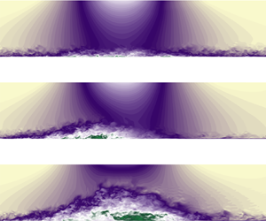





1. Introduction
Almost all turbulent boundary-layer (TBL) flows of practical relevance are subject to pressure gradients, usually introduced by changes in geometry. The pressure gradient might be favourable (FPG) or adverse (APG), and both conditions are ubiquitous in engineering and physical systems such as wings, turbomachinery and geophysical applications. A strong APG may lead to flow separation. In diffusers and turbine blades, for instance, the formation of a closed recirculation region (referred to as a ‘turbulent separation bubble’, TSB) caused when the flow suddenly separates and reattaches on the wall, is associated with a loss of efficiency and a drop in performance. In many cases, however, (e.g. helicopter blades, turbine blades, swimming fish, pitching airfoils etc.) the pressure gradient varies both spatially and temporally. The study of the separating flow caused by an unsteady pressure gradient on a flat plate will be the focus of this paper. In the rest of this section, the literature most closely related to the present work will be reviewed, first for the steady, and then for the unsteady case. Subsequently, the objectives of this study will be discussed, followed by an outline of the rest of the paper.
1.1. Steady pressure-induced separation
Many experiments focused on investigating geometry-induced separating flows (e.g. flow over a backward-facing step or a bluff body) in which the separation point is fixed in space (Simpson Reference Simpson1989). We will focus, instead, on pressure-induced separating flows, in which the free-stream velocity distribution causes strong pressure gradients on the wall, leading eventually to the formation of a closed separation bubble. For instance, Samuel & Joubert (Reference Samuel and Joubert1974) investigated a spatially developing TBL under increasing APG and noted that the mean-velocity profile develops a larger outer-wake region as the strength of the APG increases. Perry & Fairlie (Reference Perry and Fairlie1975) fixed the shape of the flexible roof of the duct and generated a pressure field that induced the formation of a closed separation bubble. Their inviscid model for turbulent separation was shown to be capable of predicting the gross properties of the flow fields. Another example involves extensive measurements of a separating turbulent boundary layer under an airfoil-type pressure distribution; see Simpson, Strickland & Barr (Reference Simpson, Strickland and Barr1977). Here, important features caused by the APG on a TBL were highlighted. It was found that the law-of-the-wall velocity-profile scaling is valid up to the intermittent separation region, and that the separated flow shares common characteristics with a free-shear mixing layer.
Results from early experiments on separated turbulent boundary layers and their underlying physical features were collected in the comprehensive and complete review papers by Simpson (Reference Simpson1981, Reference Simpson1985, Reference Simpson1987, Reference Simpson1989). It is now widely accepted that the word separation refers to an entire process that extends in space. Three regions can be identified: intermittent detachment (instantaneous backflow  $1\,\%$ of the time); transitory detachment (instantaneous backflow $50\,\%$ of the time); and detachment, which occurs (on a smooth surface) when the time-averaged wall shear stress goes to zero ( $\bar {\tau }_w=0$). Na & Moin (Reference Na and Moin1998) among others also used the mean dividing streamline ( $\psi =0$) to identify the separation point, and found good agreement with the location corresponding to zero wall shear stress.
Patrick (Reference Patrick1985) performed an experimental study of a large-scale separation bubble on a flat plate. It was observed that the reattachment region was highly unstable and characterized by low-frequency, non-periodic flapping caused by the advection of large eddies downstream of the reattachment location. This analysis was taken further by the recent investigations by Weiss, Mohammed-Taifour & Schwaab (Reference Weiss, Mohammed-Taifour and Schwaab2015) and Mohammed-Taifour & Weiss (Reference Mohammed-Taifour and Weiss2016) who analysed the unsteady behaviour of an incompressible, massively separated TBL generated by a combination of FPG and APG. They corroborated the findings of Patrick (Reference Patrick1985) and observed that the TSB was characterized by two distinct, unsteady time-dependent phenomena: a breathing motion (contraction–expansion) of the TSB at low frequency, and a medium-frequency shedding motion of turbulent structures downstream of the TSB.
Coleman & Spalart (Reference Coleman and Spalart1993) were among the first to perform a direct numerical simulation (DNS) of a weakly separated turbulent boundary layer on a flat plate. Although their inflow velocity profile was not perfectly developed (due to Reynolds number limitations), they were able to draw significant conclusions: the severe effects of flow separation on the flow physics not only affect the boundary-layer assumption but also several assumptions often used in turbulence modelling, therefore highlighting the urge of a thorough study of this type of flows.
Of particular note is the work conducted by Na & Moin (Reference Na and Moin1998) on a massively separated TBL with an inflow Reynolds number (based on momentum thickness) of  $Re_\theta =300$. The generation of a steady, closed TSB was achieved by imposing a suction–blowing velocity profile at the top boundary of the domain, a condition that set the standard for many following studies (Abe Reference Abe2017; Wu & Piomelli Reference Wu and Piomelli2018). They found that both detachment and reattachment points were not fixed in space but fluctuating upstream and downstream, and observed that flow detachment occurred over a region rather than a point. Using different definitions of the mean separation point from Simpson (Reference Simpson1989), they found good agreement between the mean dividing streamline ( $\psi =0$) and the location of zero mean wall shear stress.
More recent simulations of separated TBLs have reached higher Reynolds numbers, and use longer computational domains to promote flow development. Abe (Reference Abe2017) analysed wall-pressure fluctuations of a TSB over a flat plate for a range of Reynolds numbers up to  $Re_\theta = 900$, using a numerical methodology similar to that of Na & Moin (Reference Na and Moin1998). Particular importance was given to the Reynolds number dependence of wall-pressure fluctuations.
Wu & Piomelli (Reference Wu and Piomelli2018) performed a large-eddy simulation (LES) of a TBL over smooth and rough walls. They observed that streamline detachment occurred earlier for the rough case, and that due to the momentum deficit caused by the roughness, the separation region was significantly larger compared with the smooth case.
Continuing their early work in 1997, Coleman, Rumsey & Spalart (Reference Coleman, Rumsey and Spalart2018) performed DNS of several TBL cases with the formation of a small closed TSB in the domain. By changing both the magnitude of the pressure gradients and the Reynolds number, they were able to generate an extensive dataset with the objective of improving turbulence modelling capabilities. Extra care this time was put to have a well-developed turbulent inflow boundary condition and a longer domain to allow flow development downstream of the pressure-gradient region.
1.2. Unsteady pressure-induced separation
While the studies cited above consider pressure gradients that vary only spatially, in many cases the pressure gradient is unsteady. As described by Simpson (Reference Simpson1989) the term unsteady here refers to an organized time-dependent motion, in contrast to the inherently unsteady aperiodic character of turbulence. The focus here is on flows in which the unsteadiness is generated by applying a periodic boundary condition on the TBL.
Based on dimensional analysis the most important parameter governing the unsteadiness is the reduced frequency,  $k$, defined as
 \begin{equation} k = {{\rm \pi} f L}/{U}, \end{equation}
where  $f$ is the imposed frequency of the perturbation, $L$ represents the characteristic length scale of the problem and $U$ the velocity scale. The reduced frequency represents the ratio between the convective time scale of the flow, and the imposed unsteady time scale (Schatzman & Thomas Reference Schatzman and Thomas2017).
The response of the flow to the unsteadiness is greatly dependent on the reduced frequency,  $k$, and threshold values have been identified by Leishman (Reference Leishman2006) in his work on helicopter aerodynamics. A reduced frequency $k=0$ corresponds to nominally steady flow. When $0< k<0.05$ the flow is generally considered to be quasi-steady. As the reduced frequency grows larger the effects associated with acceleration dominate the flow physics. To be noted is the existence of two sources of ambiguity: (i) the length scale $L$ is highly dependent on the specific problem, and its choice is arbitrary in the case of a flat-plate TBL, (ii) the velocity scale $U$, in the case of rotor dynamics, is continuously changing. Therefore, the specific numbers for reduced frequency limits mentioned above should not be considered universal.
Many researchers, starting in the late 1950s worked on quantifying unsteady effects on the flow field by carrying out experiments using free-stream perturbations and by varying the reduced frequency  $k$. The common conclusion reached by several investigations (Karlsson Reference Karlsson1959; Schachenmann & Rockwell Reference Schachenmann and Rockwell1976; Kenison Reference Kenison1978; Parikh, Reynold & Jayaraman Reference Parikh, Reynold and Jayaraman1982; Simpson, Shivaprasad & Chew Reference Simpson, Shivaprasad and Chew1983; Brereton, Reynolds & Jayaraman Reference Brereton, Reynolds and Jayaraman1990) was that the mean-velocity profile is nearly unaffected by the free-stream unsteadiness over a wide range of reduced frequencies, testifying to the robustness of the mean structure of a TBL.
Covert & Lorber (Reference Covert and Lorber1984) performed measurements of an unsteady TBL over a NACA0012 airfoil for a wide range of reduced frequencies and several APGs. They found that mean profiles were nearly independent of the reduced frequency in a mild APG. However, for an APG strong enough to cause incipient separation, differences arose in the velocity profile as the frequency was increased.
In their recent work Schatzman & Thomas (Reference Schatzman and Thomas2017) experimentally investigated an unsteady APG turbulent boundary layer at a reduced frequency  $k\approx 0.12$. They showed that, for an APG strong enough to generate an inflectional velocity profile, the flow was then dominated by the existence of an embedded shear layer closely related to the inviscid instability of the outer inflection point. Using the scaling parameters of the embedded shear layer, they were able to obtain similarity of both mean and phase-averaged velocity profiles. Finally, they conjectured that the embedded shear layer might be a generic characteristic of all APG turbulent boundary layers.
One important feature of unsteady separating TBLs is that an oscillating cycle of APG and FPG can generate transient (or dynamic) flow separation that is significantly different from the steady case. Common to airfoils in manoeuvring procedures, turbine blades and helicopter rotor blades, dynamic flow separation is associated with a drop in performance and the onset of dynamic stall (Leishman Reference Leishman2006; Rival & Tropea Reference Rival and Tropea2010; Williams et al. Reference Williams, An, Iliev, King and Reißner2015). Transient separation has been the subject of many experimental studies and was found to be the reason behind the existence of dynamic hysteresis in the lift-force and pitching-moment curves (Williams et al. Reference Williams, An, Iliev, King and Reißner2015). From a fluid dynamics perspective, dynamic hysteresis is observed when a physical quantity assumes two different values at corresponding phases in a periodic cycle, and it is often used in unsteady aerodynamics to characterize the behaviour of the lift and drag coefficients for a cycle of varying angle of attack (Rival & Tropea Reference Rival and Tropea2010; Williams et al. Reference Williams, Reßiner, Greenblatt, Müller-Vahl and Strangfeld2017).
McCroskey (Reference McCroskey1982) reviewed results of experiments and numerical simulations of unsteady flows over pitching airfoils with particular emphasis on unsteady separation and dynamic stall. He showed that dynamic stall will occur on any airfoil (or other lifting device) subject to sufficiently fast, time-dependent motions (e.g. pitching, plunging, etc.) that takes the angle of attack rapidly above its static stall value. The flow physics in these conditions has been shown to be drastically different from the same airfoil under steady flow conditions. Moreover, if the angle of attack oscillates about the static stall angle, the characteristic fluid dynamic forces and moments are affected by large hysteresis effects (McCroskey Reference McCroskey1982; Simpson Reference Simpson1989).
The presence of hysteresis effects, and the associated deterioration of aerodynamic performance, have been the subject of several subsequent studies (Lissaman Reference Lissaman1983; Selig et al. Reference Selig, Guglielmo, Broern and Giguere1996; Ekaterinaris & Platzer Reference Ekaterinaris and Platzer1998). It was found that, depending on the Reynolds number, two types of separation bubble were formed over the airfoil denoted as long and short bubbles for low and high Reynolds numbers, respectively. The increasing hysteresis effects were found to have different characteristics depending on whether they were generated by long or short separation bubbles. Moreover, the magnitude of the hysteresis, and the shape of the hysteresis loops varied in a highly nonlinear manner with the amplitude of the oscillation, mean angle of attack and reduced frequency of the airfoil.
Rival & Tropea (Reference Rival and Tropea2010) experimentally analysed the effects of reduced frequency  $k$ and angle of attack on a dynamic airfoil for simple and combined pitching and plunging motions. When $k$ was increased from 0.05 to 0.1 the hysteresis curve was observed to switch from clockwise to the counter-clockwise rotation, representing an increase in the total aerodynamic lag.
Williams et al. (Reference Williams, An, Iliev, King and Reißner2015) carried out wind tunnel experiments of a pitching airfoil and showed that the lift coefficient, when transient separation occurs, exhibits dynamic hysteresis. The hysteresis was found to be highly dependent on the pitching manoeuvre, pitching frequency and flow separation. Moreover, the hysteresis loop was observed to change its shape as the frequency was increased and was present at both high and low pitching rates, which justifies the conclusion that dynamic stall (happening at high frequencies) is not a necessary condition for dynamic hysteresis (Williams et al. Reference Williams, An, Iliev, King and Reißner2015).
The onset of dynamic stall influences the behaviour of the detached flow region. In many cases the stalled flow region was found to be highly unstable: Mullin, Greated & Grant (Reference Mullin, Greated and Grant1980) reported that Lebouche and Martin performed an experiment in which the unsteadiness was tested by pulsating the incoming flow in a duct with enlargements on both sides to generate symmetric flow separation. They found a limiting value of reduced frequency  $k$ below which the recirculation vortex was shed downstream. In their own experiment of a pulsating flow over a backward-facing step, Mullin et al. (Reference Mullin, Greated and Grant1980) corroborated the findings by Lebouche and Martin and found that the separated-flow region behind the step was strongly perturbed by the free-stream oscillation, and then finally advected downstream.
In a review paper on separated flows, Simpson (Reference Simpson1989) described the occurrence of dynamic stall in a diffuser. Even in this case, the stalled-fluid region grows in the wall-normal direction, becomes unstable and is washed out of the diffuser.
The literature on unsteady flows studied via numerical simulations is also quite substantial, especially for the case of a pitching airfoil. However, the spatially developing TBL under the effect of unsteady pressure gradients, with alternating APG and FPG has been the subject of fewer studies. In the following, we summarize only those most relevant to our work.
Spalart & Baldwin (Reference Spalart and Baldwin1989) performed a DNS of a turbulent, oscillatory boundary layer in which the free-stream velocity  $U_\infty$ varied sinusoidally around a zero mean. A variety of flow behaviours, including the reversal of the Reynolds shear stress, were observed. Attention was given to develop a theory for the velocity and Reynolds-stress profiles at high Reynolds numbers that could improve turbulence models.
Scotti & Piomelli (Reference Scotti and Piomelli2001) carried out direct and LESs of a turbulent pulsating flow in a periodic channel. They examined a wide range of frequencies and pressure gradients. From the study of the phase-averaged quantities they noticed the presence of waves that originate in the viscous and buffer layers and propagate away from the wall. They also introduced the concept of the turbulent Stokes length  $l_{t}$, which defines how far vorticity waves, generated near the wall, penetrate into the flow.
In their very recent investigation, Park, Ha & Donghyun (Reference Park, Ha and Donghyun2021) analysed a TBL under unsteady APGs at a reduced frequency  $k=0.625$ with the aim of testing several turbulence models ( $\mathcal {K}{-}\omega$, where $\mathcal {K}$ is the turbulent kinetic energy and $\omega$ the turbulent frequency, and Spalart–Allmaras) and provide insights into their accuracy of predicting unsteady separated flows. The APG was periodically varied to obtain dynamic separation and reattachment but the pressure-gradient distribution was always adverse to favourable and the TSB never disappeared. They found that turbulence models can qualitatively predict the formation of the separation bubble, but discrepancies were found on the phase response and near-wall behaviour.
1.3. Objectives and outline
Although much effort has been invested to shed light on the complexity of separated flows, many questions still remain unanswered. Among them are: (i) How does the reduced frequency  $k$ affect the transient separation cycle of a flat-plate TBL? (ii) What are the underling physical characteristics behind dynamic hysteresis and their consequences for the flow behaviour? (iii) Can a simulation of a TBL under unsteady pressure gradients provide valuable insights into the dynamic stall process?
The present work aims at tackling these issues, with the additional objective of creating a dataset that can be used to assess the accuracy of turbulence models. The configuration studied, a flat-plate turbulent boundary layer with imposed pressure gradient, is much simpler than what is found in practical applications, which may include streamwise and/or spanwise curvature, roughness, etc. Isolating the effect of the pressure gradient in a simplified geometry can, however, yield useful information, relevant to more complex cases. This approach has been demonstrated to give valuable insight into the physics of separation in previous studies (Na & Moin Reference Na and Moin1998; Abe Reference Abe2017; Wu & Piomelli Reference Wu and Piomelli2018). We will show, in fact, that many phenomena that characterize unsteady separation in realistic flows can be observed in this simplified configuration as well.
The paper is structured as follows. Section 2 describes the numerical set-up (governing equations, boundary conditions, unsteadiness and simulation parameters). Section 3 presents the simulation results, both for steady and unsteady pressure gradients. Results are shown for a wide range of reduced frequencies  $k$ and compared with the corresponding steady cases. Finally, § 4 contains concluding remarks and highlights possible directions for future investigations.
2. Problem formulation
2.1. Governing equations and boundary conditions
In the present work, simulations are performed using the LES technique. The incompressible Navier–Stokes equations are solved for filtered quantities (here indicated with an bar)
 $$\begin{gather} \frac{\partial \bar{u}_i}{\partial x_j}=0, \end{gather}$$
 $$\begin{gather}\frac{\partial\bar{u}_i}{\partial t} + \frac{\partial}{\partial x_j}\left(\bar{u}_i\bar{u}_j\right) ={-}\frac{\partial\bar{p}}{\partial x_i} + \nu\nabla^{2}\bar{u}_i - \frac{\partial \tau_{ij}}{\partial x_j}, \end{gather}$$
where,  $x_1$, $x_2$ and $x_3$ (or $x$,
$x$,  $y$,
$y$,  $z$) are the streamwise, wall-normal and spanwise directions, ${{\bar {u}_i}}$ (or $\bar {u}$, $\bar {v}$, $\bar {w}$) the velocity components in the coordinate directions, $\bar {p}$ is the pressure (divided by the constant density), $\nu$ is the kinematic viscosity, and $\tau _{ij} = \overline {u_i u_j} - \bar {u}_i\bar {u}_j$ is the subfilter-scale stress tensor. In the present study $\tau _{ij}$ is modelled using the Vreman eddy-viscosity model (Vreman Reference Vreman2004). The computational domain is shown in figure 1 (a black arrow denoting the flow direction). The length and velocity scales used for normalization are the boundary-layer displacement thickness and the free-stream velocity at the inflow plane, $\delta _o^{*}$ and $U_o$. The Reynolds number based on $\delta _o^{*}$ and $U_o$ is $Re_*=1000$. In the following the overline will be dropped, and $u_i$, $p$ will be used to represent the filtered velocity and pressure.
Sketch of the computational domain. A parallel auxiliary simulation is used to generate the inflow boundary condition at the desired  $Re_*$.

The inflow boundary condition is generated using an auxiliary simulation as proposed by Lund, Wu & Squires (Reference Lund, Wu and Squires1998) (figure 1). The auxiliary simulation uses the recycling/rescaling boundary conditions (also proposed in that paper) in the streamwise direction. A plane at the desired Reynolds number is extracted from the auxiliary calculation and interpolated to match the resolution and domain size of the main simulation. A convective boundary condition is prescribed at the outlet (Orlanski Reference Orlanski1976). On the bottom wall, the no-slip boundary condition is applied.
The unsteady pressure gradient is generated by imposing a vertical velocity  $V_\infty (x,t)$ at the free stream, that changes both in space and time
 \begin{equation} V_\infty (x,t)= V_o(x)\sin\left( 2{\rm \pi}\frac{t}{T}\right) = U_\infty(x,t) \frac{{\rm d}\delta^{*}}{{\rm d}\kern0.7pt x}+(\delta^{*}-L_y)\frac{{\rm d}U_\infty}{{\rm d}\kern0.7pt x}, \end{equation}
where  $T$ is the oscillation period, and $V_o$ is the streamwise distribution of wall-normal velocity, which was chosen to match the case studied by Na & Moin (Reference Na and Moin1998). Here, $\delta ^{*}$ is the displacement thickness, and $L_y$ is the domain height. This approach is analogous to the use of a contoured wind tunnel ceiling in experiments, with the far-field streamlines representative of the wind tunnel shape. The free-stream velocity in the streamwise direction, $U_\infty$, is obtained by imposing a zero-vorticity condition on the top boundary (Na & Moin Reference Na and Moin1998; Abe Reference Abe2017; Wu & Piomelli Reference Wu and Piomelli2018)
 \begin{equation} \left.\frac{\partial u}{\partial y}\right\vert_{y=L_y} =\frac{{\rm d}V_\infty}{{\rm d}\kern0.7pt x} ; \quad \left.\frac{\partial w}{\partial y}\right\vert_{y=L_y}=0. \end{equation}
2.2. Numerical method
The computational domain is  $L_x \times L_y \times L_z = 600\delta _o^{*} \times 64\delta _o^{*}\times 55\delta _o^{*}$ in all cases. The dimensions of the domain were chosen based on cases studied in the literature; the domain length, in particular, is significantly longer than that used by Na & Moin (Reference Na and Moin1998) and Abe (Reference Abe2017). This length is sufficient to ensure a relaxation of the boundary layer towards equilibrium in all the steady cases. A uniform grid in the streamwise and spanwise directions, and a stretched grid in the wall-normal direction, are employed. A grid-convergence study was performed (which will be described momentarily) and the final grid uses $N_x\times N_y\times N_z = 1536\times 192\times 256$ points. In wall units (defined using the friction velocity $u_{\tau }$ at the inflow plane) we have $\Delta x^{+}=18.7$, $\Delta y^{+}_{min}=0.7$ and $\Delta z^{+}=10$, values comparable to direct numerical simulations for both APGs (Na & Moin Reference Na and Moin1998) and zero pressure gradient (ZPG) (Spalart Reference Spalart1988; Schlatter & Örlü Reference Schlatter and Örlü2010).
The governing equations (2.1)–(2.2) are solved using second-order accurate central differences in space on a staggered grid. The fractional-step method is used for time advancement (Chorin Reference Chorin1968; Kim & Moin Reference Kim and Moin1985). A second-order accurate semi-implicit time-advancement method is used in which the Crank–Nicolson scheme is employed for the wall-normal diffusive terms, while a low-storage third-order Runge–Kutta scheme is applied to the remaining terms. The Poisson equation is solved directly using a fast Fourier transform in the spanwise direction, a fast cosine transform in the streamwise direction and a direct solver for the resulting tridiagonal matrix in the wall-normal direction. The code is parallelized using the message-passing interface and has been well validated and previously applied to similar cases (Keating et al. Reference Keating, Piomelli, Bremhorst and Nešić2004; Yuan & Piomelli Reference Yuan and Piomelli2015; Wu & Piomelli Reference Wu and Piomelli2018).
A grid-convergence study has been carried out for a steady APG case, with the free-stream wall-normal velocity corresponding to the strongest APG. Figure 2 shows the free-stream velocity  $U_\infty$ and the streamwise mean-velocity profiles at three locations in the domain. The grid mentioned above was compared with a coarser one using $1152\times 129\times 152$ points; the difference in the mean velocity is less than $2\,\%$. Reynolds stresses were also compared (not shown here) and showed good agreement. Finally, figure 3 shows the wall-pressure and skin-friction coefficients
 \begin{equation} C_p = \frac{2\left(P_{w} - P_{w,o}\right)}{U_o^{2}};\quad C_f = \frac{2\tau_w}{\rho U_o^{2}} \end{equation}
for the two grids compared with reference data from the literature; the present LES results are within  $4\,\%$ of the DNS data; the difference from the pressure coefficient measured by Weiss et al. (Reference Weiss, Mohammed-Taifour and Schwaab2015) using a low-speed, open-circuit, blower boundary-layer wind tunnel is probably due to a slight difference in the blowing section of the transpiration velocity profile $V_\infty$. The difference in $C_f$ between the present data and those by Abe (Reference Abe2017) is probably due to the chosen length of the computational domain. In the present study $100\delta _o^{*}$ are left for flow development before and after the pressure gradient region. The domain used by Abe (Reference Abe2017), on the other hand, was considerably shorter, and most importantly did not include a recovery length in which the pressure gradient was nominally zero.
(a) Free-stream velocity  $U_\infty$ (black lines represent the locations where the velocity profiles are extracted), and (b) mean velocity at three different streamwise locations. Blue lines denote the $1536\times 192\times 256$ grid; red lines denote the $1152\times 129\times 152$ grid.

Distribution of (a) the mean pressure coefficient  $C_p$ and (b) the skin-friction coefficient $C_f$. Blue dashed line, $1536\times 192\times 256$ mesh; red dashed line, $1152\times 129\times 152$ mesh; $\square$ Abe (Reference Abe2017); $\circ$ Weiss et al. (Reference Weiss, Mohammed-Taifour and Schwaab2015).

2.3. Simulation parameters
The unsteadiness was imposed by modulating the wall-normal free-stream velocity using a sine function. We define a phase angle  $\varPhi =2{\rm \pi} (t+nT)/T$ (with integer $n$). Figure 4 shows the free-stream streamwise velocity distribution at four phases. At $t=nT$ or $\varPhi =0^{\circ }$ and $t=(n+1/2)T$ or $\varPhi =180^{\circ }$ the pressure gradient is nominally zero. For $180<\varPhi <360^{\circ }$ the free-stream velocity first decreases (causing an APG) and then returns to its inflow value (causing a FPG). The maximum APG is achieved at $\varPhi =270^{\circ }$. Conversely, for $0<\varPhi <180^{\circ }$ a FPG is followed by an APG, the maximum FPG occurring at $\varPhi =90^{\circ }$.
Free-stream velocity at four phases in the cycle. Black arrows denoting the direction of incrementing phase angle  $\varPhi$.

For post-processing, the oscillation period was divided into 20 equally spaced phases; figure 4 shows the phase angle  $\varPhi$ and the free-stream streamwise velocity $U_\infty$ profiles at four different phases during one complete cycle. For brevity, we will refer to the phases $0^{\circ }<\varPhi <90^{\circ }$ as the ‘ZPG–FPG phases’ (although an APG is present following the FPG). Similarly, the ‘FPG–ZPG phases’ correspond to $90^{\circ }<\varPhi <180^{\circ }$, the ‘ZPG–APG phases’ to $180^{\circ }<\varPhi <270^{\circ }$ and the ‘APG–ZPG phases’ to $270^{\circ }<\varPhi <360^{\circ }$. We will also refer to the ‘separation side’ and ‘acceleration side’ of the cycle, for $180^{\circ }<\varPhi <360^{\circ }$ and $0^{\circ }<\varPhi <180^{\circ }$, respectively.
As previously mentioned, the non-dimensional parameter that characterizes the unsteadiness in our problem is the reduced frequency  $k$, defined here as
 \begin{equation} k=\frac{{\rm \pi} f L_{PG}}{U_{o}}, \end{equation}
where  $f=1/T$ is the imposed frequency, $L_{PG}$ is a characteristic length and $U_{o}$ is the free-stream velocity at the inflow plane. In many cases the length-scale definition is clear: for a pitching airfoil, for instance, it is the chord length; for a swimming fish it would be the length of the body. Here, on the other hand, some arbitrariness exists. We have chosen to use the length over which the pressure gradient varies as the analogue of the chord length. Some arbitrariness still remains (we chose $L_{PG}$ as the distance over which $|V_o|>0.06 \max (|V_o|)$, so that a direct comparison with the literature is not possible. However, the results do show trends that are in agreement with the literature, as will be shown in the following sections. We performed numerical simulations for $k=0.2$, $1$ and $10$ to represent a wide range of physical behaviours; from a very fast flutter-like motion, to a slower quasi-steady flapping. As mentioned in § 1, the non-dimensional reduced frequency represents the ratio between the convective time scale of the flow, and the imposed unsteady time scale of the perturbation. Given that in our case the convective time scale is constant, the reduced frequency is the only parameter that governs the unsteady pressure gradient. Leishman (Reference Leishman2006) found that a reduced frequency $k>0.05$, when the imposed time scale is less than 20 convective time scales, was the threshold beyond which the boundary layer was clearly unsteady, and many experimental studies have been carried out for a wide range of reduced frequencies $0.1< k<82$ (Karlsson Reference Karlsson1959; Brunton & Rowley Reference Brunton and Rowley2009).
To analyse the results all quantities were first averaged in the homogeneous spanwise direction. Then two averaging procedures were used: time averaging (indicated with an overline), and phase averaging (indicated with angle brackets). The time- and phase-averaging operators are defined respectively as
 \begin{align} \bar{f}(x,y) = \lim_{T\longrightarrow\infty} \frac{1}{T}\int_{0}^{T}f\left(x,y,t\right){\rm d}t; \quad \left\langle f\left(x,y,t\right)\right\rangle = \lim_{N\longrightarrow\infty} \frac{1}{N}\sum_{n=0}^{N}f\left(x,y,t+n\tau\right). \end{align}
Using these averaging operators, triple decomposition (Hussain & Reynolds Reference Hussain and Reynolds1970) could be employed. Every instantaneous quantity is decomposed into a time-averaged component, a coherent (or periodic) component and a stochastic (or turbulent) component
 \begin{equation} f\left(x,y,z,t\right) = \bar{f}\left(x,y\right) + \tilde{f}\left(x,y,t\right) + f'\left(x,y,z,t\right), \end{equation}
where the tilde denotes the coherent component. From (2.8), several relations follow that connect the various components of the field
 \begin{equation} \left\langle f\right\rangle=\bar{f}+\tilde{f}; \quad f=\left\langle f\right\rangle+f'; \quad f'=f-\left\langle f\right\rangle ; \quad \tilde{f}=\left\langle f\right\rangle-\bar{f}. \end{equation}
We also carried out numerical simulations with a steady pressure gradient corresponding to that imposed at  $\varPhi =0^{\circ }$, $54^{\circ }$, $90^{\circ }$, $270^{\circ }$ and $306^{\circ }$. The Reynolds number chosen for the present numerical simulation: $Re_{*}=1000$ was consistent with similar previous investigations (Abe Reference Abe2017; Coleman et al. Reference Coleman, Rumsey and Spalart2018). Phase-averaged statistics were accumulated over several periods, dependent on the reduced frequency. To estimate the uncertainty of the results in terms of sample convergence, we compared the phase-averaged velocity obtained by using only half of the cycles with that obtained using all the available ones. For the $k=0.2$ case (which is the most critical one, since the period is longer and fewer cycles could be computed) the difference is less than 3 %, whereas in the other cases it is less than 1 %.
3. Results
3.1. Steady pressure-gradient calculations
To characterize the influence of the unsteady pressure gradient on the flow physics, five cases in which the pressure gradient is steady have been analysed for direct comparison. Following the notation introduced in the previous section, and as illustrated in figure 4, these cases correspond to the pressure gradients imposed at  $\varPhi =270^{\circ }$, $306^{\circ }$, $0^{\circ }$, $54^{\circ }$ and $90^{\circ }$, and will be referred to as SC-1 through SC-5. In cases SC-1 and 2 an APG is followed by an FPG, whereas in cases SC-4 and 5 the reverse happens. SC-3 is the ZPG case.
Figure 5 shows contours of the streamwise time-averaged velocity  $\bar {u}$ for the steady cases characterized by a non-zero pressure gradient (SC-1, SC-2, SC-4, SC-5). In both SC-1 and SC-2 cases the APG generated by the suction side of the $V_\infty$ velocity profile leads to flow separation. In the SC-1 case, the closed separation bubble formed has characteristics similar to those described in previous numerical studies (Na & Moin Reference Na and Moin1998; Abe Reference Abe2017; Wu & Piomelli Reference Wu and Piomelli2018).
Contours of streamwise time-averaged velocity  $\bar {u}$ for the steady calculations corresponding to the following phases: (a) SC-1 $\varPhi =270^{\circ }$; (b) SC-2 $\varPhi =306^{\circ }$; (c) SC-4 $\varPhi =54^{\circ }$; (d) SC-5 $\varPhi =90^{\circ }$. Solid and dashed lines denote positive and negative values of the streamfunction, respectively.

For the SC-1 case, the height of the separation bubble is approximately  $23\delta _o^{*}$ and its length, identified by the mean separation streamline, is approximately $120\delta _o^{*}$. SC-4 and SC-5 cases both experience a strong FPG given by the blowing side of the velocity profile before the APG section, as can be clearly observed by the streamline curvature in figure 5(c,d). As a result, in both cases no reversed flow is observed.
Figure 6 shows the streamwise distribution of the time-averaged skin-friction coefficient  $C_f$. In both SC-1 and SC-2 cases $C_f$ is negative over a portion of the domain. In the SC-1 case the length over which $C_f\leqslant 0$ is approximately $120\delta _o^{*}$, consistent with the separated-flow region length estimated using the mean separation streamline.
Spatial distribution of the skin-friction coefficient  $C_f$ for the steady calculations corresponding to the following phases: blue solid line, SC-1 $\varPhi =270^{\circ }$; red dashed line, SC-2 $\varPhi =306^{\circ }$; green dotted line, SC-3 $\varPhi =0^{\circ }$; orange dotted line, SC-4 $\varPhi =54^{\circ }$; purple dash-dotted line, SC-5 $\varPhi =90^{\circ }$.

The SC-4 and SC-5 cases are characterized by an initial increase of the skin-friction coefficient due to the acceleration. The SC-3 case (symbols) has the characteristic behaviour of a ZPG TBL in equilibrium conditions. In the  $100\delta _o^{*}$ upstream of the pressure-gradient region, subject to a ZPG, all the cases match, indicating that the pressure gradient imposed by the free-stream vertical velocity $V_\infty$ does not affect the inflow region.
While the SC-1 and SC-2 cases recover to roughly the ZPG value of  $C_f$ after the reattachment point, the SC-4 and SC-5 cases show a drastic drop in the $C_f$ magnitude of approximately 38 %. The acceleration induced by the FPG side of the velocity profile $V_\infty$ gives the flow enough energy to resist flow separation, but the following APG is strong enough that the flow does not completely recover and the boundary-layer characteristics are still changing in the outflow region. A common characteristic, resulting from the imposed pressure gradient, is that every case is significantly far from the equilibrium condition, even in the outflow region.
3.2. Dynamic pressure-gradient calculations
3.2.1. Time-averaged velocity field
As mentioned in § 2, a total of three unsteady pressure-gradient cases have been analysed. They are denoted as UPG-1 (with  $k=10.0$), UPG-2 ( $k=1.0$) and UPG-3 ( $k=0.2$). The first result that will be presented here is the time-averaged behaviour of the velocity over the cycle. As discussed in § 1, many researchers found that the time-averaged quantities are insensitive to the reduced frequency $k$. Figure 7 shows the time-averaged streamwise velocity $\bar {u}$ in wall units (indicated by $+$) for the dynamic cases compared with the steady ZPG case at three different streamwise locations, one upstream of the recirculation region, one at its centre and one downstream of the pressure-gradient region. Wall units are obtained by normalizing the velocity field using the friction velocity $u_\tau =(\tau _w/\rho )^{1/2}$ and the viscosity $\nu$.
Time-averaged profiles of streamwise velocity in wall units for the dynamic cases compared with the steady ZPG case at three streamwise locations. Symbols denote the steady calculations. Colours are as follows:  $\bullet$ steady case; green solid line, $k=10$; blue dashed line, $k=1$; orange dash-dotted line, $k=0.2$.

First, we observe that the time-varying free-stream pressure distribution does not affect the region upstream of the pressure gradient, indicating that the ZPG region is fully developed, and unaffected by the pressure gradient. Secondly, in contrast with previous studies, the effect of the unsteady pressure gradient on the time-averaged fields at the centre of the pressure-gradient region is significant. The discrepancy with previous experimental observations is mainly due to a Reynolds number effect. The acceleration parameter,
 \begin{equation} K=\frac{\nu}{U_\infty^{2}}\frac{{\rm d}U_\infty}{{\rm d}\kern0.7pt x}, \end{equation}
which characterizes the strength of the APG, depends on the viscosity (or, equivalently, the Reynolds number). For a given free-stream velocity distribution, an intermediate- $Re$ simulation will present much stronger pressure-gradient effects than observed in the experiments, which are at much higher $Re$.
$Re$.
The UPG-1 case maintains the conventional shape of a TBL but the logarithmic region is shifted downwards compared with the steady ZPG case. This effect is often associated with the presence of an APG (Spalart & Watmuff Reference Spalart and Watmuff1993; Monty, Harun & Marusic Reference Monty, Harun and Marusic2011). Furthermore, both the medium-frequency (UPG-2) and the low-frequency (UPG-3) cases display an intensification of the wake region in the centre of the pressure-gradient region, another common consequence of the APG. Unlike the UPG-1 case, the logarithmic region for the UPG-2 case is shifted above the classic TBL log law. Finally, close to the end of the computational domain (in a region in which the free-stream velocity does not change with time) significant differences can still be observed. The high-frequency case has returned to the equilibrium, ZPG profile, and the low-frequency one is approaching it. The intermediate-frequency case, on the other hand, still displays some discrepancies in the wake region; the physical reasons behind this behaviour will be explained in the following section.
3.2.2. Flow evolution
Figure 8 shows profiles of streamwise and wall-normal phase-averaged velocity at the free stream,  $\langle U_\infty \rangle,\langle V_\infty \rangle$ for each frequency for four equally spaced phases $\varPhi$ in the cycle: $0^{\circ }$ (ZPG – corresponding to SC-3 case), $90^{\circ }$ (corresponding to the SC-5 case), $180^{\circ }$ (ZPG – corresponding to the SC-3 case) and $270^{\circ }$ (corresponding to the SC-1 case). Comparison is made with steady calculations at the same phases.
Profiles of free-stream streamwise  $\langle U_\infty \rangle$ and wall-normal $\langle V_\infty \rangle$ phase-averaged velocity. Only the main four phases of the cycle are shown (see figure 4). Symbols denote the steady calculations, lines represent dynamic results at different reduced frequencies $k$. Solid lines $U_\infty$, dashed lines $V_\infty$. Colours are as follows: $\bullet$ steady case; green lines, $k=10$; blue lines, $k=1$; orange lines, $k=0.2$.

The medium-frequency case (UPG-2) shows some differences in  $\langle U_\infty \rangle$ at the centre of the domain for $\varPhi =0^{\circ }$, and further downstream for $\varPhi =90^{\circ }$. To explain this behaviour, figures 9, 10 and 11 show contours of phase-averaged streamwise velocity $\langle u\rangle$ for the same four phases in the cycle. It should be noted here that, in the unsteady simulations, the size of the recirculation bubble is not the same as in the steady ones. This results in a different value of the mean velocity in the region of the recirculation bubble, and a different development of $\delta ^{*}$. Although the forcing (the wall-normal velocity) is the same for steady and unsteady cases, the free-stream velocity $U_\infty$ may be different; this is especially noticeable for the intermediate frequency.
Contours of phase-averaged streamwise velocity  $\langle u\rangle$ for $k=10$. Only the main 4 phases of the cycle are shown.

Contours of phase-averaged streamwise velocity  $\langle u\rangle$ for $k=1$. Only the main four phases of the cycle are shown.

Contours of phase-averaged streamwise velocity  $\langle u\rangle$ for $k=0.2$. Only the main four phases of the cycle are shown.

In the UPG-1 case, the two ZPG phases ( $0^{\circ }$ and $180^{\circ }$) show the usual behaviour of a flat-plate TBL and there is little difference in the outer layer and in the far stream. At phase $\varPhi =90^{\circ }$, we observe the accelerating flow region due to the FPG and the corresponding decrease of the boundary-layer thickness, which increases again in the APG section; the flow then redevelops towards a ZPG TBL at the outlet. At phase $\varPhi =270^{\circ }$, the rate of change of the free-stream forcing $V_\infty$ is fast enough to prevent the growth of the separation bubble to dimensions comparable to the steady case SC-1. However, flow separation occurs in a very small region close to the wall and the length of the separation region is comparable to the one observed in SC-1.
Figure 10 shows the phase-averaged streamwise velocity  $\langle u\rangle$ for the medium-frequency case UPG-2. As the reduced frequency $k$ decreases, the thickness of the separation bubble increases but the length of the separation region is significantly reduced (see $\varPhi =270^{\circ }$ figure 10). The separation region is highly unsteady, and the stalled fluid generated by the reversed flow is advected downstream and periodically washed out of the domain (Simpson Reference Simpson1989). This behaviour is consistent with experimental observations by Mullin et al. (Reference Mullin, Greated and Grant1980) who analysed a flow over a backward-facing step using a sinusoidal oscillation of the free stream with an amplitude $12\,\%$ of the average velocity. The reduced frequency $F^{*}=fh/\bar {U}$, defined as a function of the step height $h$ and mean velocity $\bar {U}$, was specifically chosen to be smaller than the threshold value of $F^{*}=0.07$. Mullin et al. (Reference Mullin, Greated and Grant1980) in fact mentioned a previous experiment carried out by Lebouche and Martin of a similar pulsating flow in which it was observed that when the frequency was reduced below $F^{*}=0.07$ the re-circulation vortex was shed (Mullin et al. Reference Mullin, Greated and Grant1980; Simpson Reference Simpson1989). Present results corroborate findings by Mullin et al. (Reference Mullin, Greated and Grant1980) and Lebouche and Martin and show that there is a limiting reduced frequency $1 < k < 10$ below which the stalled-fluid region is advected downstream, causing the hysteresis effects to move away from the wall. The fact that the two ZPG phases ( $\varPhi =0^{\circ }$ and $\varPhi =180^{\circ }$) differ indicates the presence of hysteresis, which will be discussed later.
As the reduced frequency is further decreased (figure 11), the separation bubble (at  $\varPhi =270^{\circ }$) grows to dimensions comparable (both in height and length) to the steady case, indicating a trend towards a quasi-steady state. Some differences between the two ZPG phases ( $\varPhi =0^{\circ }$ and $\varPhi =180^{\circ }$), however, indicate that hysteresis effects are still present as the thickness of the boundary layer is significantly different. In this case, the separation region appears to be more stable, compared with the UPG-2 case; however, advection of turbulent structures downstream of the reattachment point is still a dominant physical mechanism and causes the aforementioned hysteresis. Figure 12 shows contours of phase-averaged streamwise velocity $\langle u\rangle$ at phase $\varPhi =270^{\circ }$ for the unsteady cases and the corresponding steady case SC-1, panel (d).
Contours of phase-averaged streamwise velocity  $\langle u\rangle$ for the phase $\varPhi =270^{\circ }$: (a) $k=10$; (b) $k=1$; (c) $k=0.2$; (d) steady calculation (SC-1). Solid and dashed lines denote positive and negative values of the streamfunction, respectively.

Table 1 summarizes the dimensions of the separation bubbles; here,  $X_S$ and $X_R$ are the averaged separation and reattachment locations.
Dimensions of the four separation bubbles for the unsteady and steady (SC-1) cases.

To quantify the strength of the pressure gradient we used the ratio of the pressure velocity  $U_p=[({\rm d}P_{\infty }/{{\rm d}\kern0.7pt x})\delta ^{*}]^{1/2}$ to the free-stream streamwise velocity $U_\infty$, as defined in Kitsios et al. (Reference Kitsios, Sekimoto, Atkinson, Sillero, Borrell, Gungor, Jiménez and Soria2017), shown in figure 13. We observe the persistence of pressure-gradient effects, in the region where the flow separates, even in the two ZPG phases. This behaviour will be explained in a following section. At $\varPhi =90^{\circ }$, where the FPG precedes the APG and $U_\infty > 1$, there is very good agreement between dynamic and steady cases, and we observe that in the pressure-gradient region ( $150< x/\delta _o^{*}<450$) the ratio $U_p/U_\infty$ is positive but lower than 1, implying that convection effects overcome the pressure gradient. On the other hand, at phase $\varPhi =270^{\circ }$, where the APG precedes the FPG and $U_\infty <1$ the opposite occurs. The UPG-3 case shows very good agreement with the corresponding steady case, and in the separation region pressure-gradient effects mildly overcome the convection ones. At high and intermediate frequencies (UPG-1, UPG-2) there is a very good match with the corresponding steady case upstream and downstream of the separation region; however, pressure-gradient effects are significantly greater than convection effects in the centre of the domain. This behaviour is closely related to that shown in figure 8, and deeply affects the flow physics, as will be shown momentarily.
Streamwise distribution  $U_p/U_\infty$. Only the main four phases of the cycle are shown. Colours are as follows: $\bullet$ steady case; green solid line, $k=10$; blue dashed line, $k=1$; orange dash-dotted line, $k=0.2$.

Finally, figure 14 shows the streamwise phase-averaged velocity profile at four phases in the cycle for the different reduced frequencies at three streamwise locations:  $x/\delta _o^{*}=270$, $300$ and $450$, upstream, at the centre and downstream of the pressure-gradient region. The phenomena described above can be more clearly visualized. At $\varPhi =90^{\circ }$, where the FPG precedes the APG, the dynamic cases match reasonably well the steady calculations, with the best agreement being the quasi-steady low-frequency (UPG-3) case. At $\varPhi =0^{\circ }$ and $\varPhi =180^{\circ }$, the two ZPG phases, we observe again that the high and low frequencies (UPG-1, UPG-3) are in agreement with SC-3 whereas the intermediate-frequency case (UPG-2) shows significant hysteresis effects, especially in the location at the centre of the separation region ( $x/\delta _o^{*}=300$). Once again, this is due to the advection of the stalled-fluid region downstream of the separation bubble, which will be discussed momentarily. Hysteresis effects will be analysed in depth in the following section.
Streamwise phase-averaged  $\langle u\rangle$ velocity profile for four phases in the cycle for the different reduced frequencies $k$ (colours) and streamwise locations (line styles). Comparison is made with steady calculations (symbols) at the same streamwise locations. Each profile is shifted by one unit for clarity. Solid line, $x/\delta _o^{*}=270$ dashed line, $x/\delta _o^{*}=300$; dotted line, $x/\delta _o^{*}=450$.

Significant differences between steady and dynamic calculations can be observed when flow separation occurs ( $\varPhi =270^{\circ }$). First, we observe the difference between the dynamic cases, which is due to the different size and development of the separation bubbles. Second, even though UPG-3 case is approaching a quasi-steady state, displaying a good match with the steady calculation, it is characterized by a stronger backflow in the centre of the separation region, indicating the persistence of transient effects. Of specific interest is the comparison between the high and intermediate frequencies (UPG-1 and UPG-2) for $\varPhi =270^{\circ }$ in the centre of the separation region (figure 14). We previously showed (figure 8) that both $\langle U_\infty \rangle$ and $\langle V_\infty \rangle$ for these cases are roughly the same throughout the domain, which suggests that the free-stream pressure gradient imposed on the flow is the same. The discrepancies in the velocity profiles near the free stream observed in figure 14 can be explained considering (2.3). While $V_\infty$ is the same for all cases, $\delta ^{*}$ changes due to the blockage caused by the separation bubble, and $U_\infty$ adjusts to ensure global mass conservation.
To highlight the transient effects present in every unsteady case, we consider the phase-averaged skin-friction coefficient  $\langle C_f\rangle$ plotted in figure 15 as a function of the streamwise direction $x/\delta _o^{*}$ and phase $\varPhi$. Phases $\varPhi =90^{\circ }$ and $\varPhi =270^{\circ }$ are the two extreme FPG and APG phases, respectively, while $\varPhi =0^{\circ }$ and $\varPhi =180^{\circ }$ are the two ZPG phases. The separated flow appears as a green elongated elliptical region, while the region of high wall stress corresponding to the acceleration phases is darker purple. At very high frequency (UPG-1 case) these two regions are tilted, indicating that the regions of high positive and negative wall stress are not only growing in magnitude, but also moving upstream in time. Also, the maximum and minimum wall stresses are shifted in $x$ with respect to each other, and areas of negative wall stress are observed in the ZPG phases. At this frequency the near-wall flow is decoupled from the free-stream forcing.
Contours of phase-averaged skin-friction coefficient  $\langle C_f\rangle$ as a function of the streamwise direction $x$ and phase $\varPhi$. Black dashed-dotted lines denote the ZPG phases: (a) $k=10$; (b) $k=1$; (c) $k=0.2$.

At  $k=1$ the contours of $\langle C_f\rangle$ are now enclosed between the two ZPG phases, and the locations of maximum and minimum correspond to $\varPhi =90^{\circ }$ and $\varPhi =270^{\circ }$, respectively. However, the shedding of the recirculation region observed at this frequency causes the $\langle C_f\rangle$ to be very small after the reattachment, and the contours of $\langle C_f\rangle$ to be tilted in the downstream region. The washing out of the slow-moving fluid appears as a lighter diagonal streak starting in the recirculation zone and propagating downstream. The convection speed of this propagation can be estimated from figure 15(b) to be approximately $0.5\,U_o$. This result is consistent with the convection velocity of the vortical disturbance over the chord length of an airfoil when dynamic stall occurs (Leishman Reference Leishman2006).
At low frequency the contours are symmetric in time, and the shedding disappeared. However, due to flow impinging the wall in the reattachment region, the location of minimum  $\langle C_f\rangle$ is now shifted downstream, occurring at $x/\delta _o^{*}=330$.
Figure 16 shows the spatial distribution of the phase-averaged skin-friction coefficient  $\langle C_f\rangle$ for four phases in the cycle for the different reduced frequencies $k$, compared with steady cases (see figure 6). First, we see that $\langle C_f\rangle$ profiles for the dynamic cases match reasonably well the steady calculation in the acceleration side of the cycle ( $\varPhi =90^{\circ }$), with the best agreement being the UPG-3 case. This trend is now consistent with previous presented results. At the two ZPG phases, both the medium (UPG-2) and low (UPG-3) frequencies match very well the steady calculation, whereas the very high-frequency case (UPG-1) displays significant differences. As mentioned earlier, at this frequency the near-wall flow behaviour is completely decoupled from the free-stream forcing, and it is interesting to note that, as opposed to the other cases, UPG-1 case is not characterized by a phase of quasi-uniform (or monotonically decreasing) $\langle C_f\rangle$.
Distribution of phase-averaged skin-friction coefficient  $\langle C_f\rangle$ for four phases in the cycle for the different reduced frequencies $k$.
$k$.  $\bullet$ Steady case; green solid line, $k=10$; blue dashed line, $k=1$; red dash-dotted line, $k=0.2$.

3.2.3. Hysteresis effects
As mentioned in § 1, dynamic hysteresis is observed when a physical quantity assumes two different values at corresponding phases in a periodic cycle. The TBL experiences the same pressure gradient twice in one cycle and, since we consider 20 equally spaced phases, we have nine matching phases (plus the two extreme ones). The phases are divided into three groups, as shown in figure 17: the first includes phases in the separation side of the cycle, where the APG precedes the FPG, and the free-stream velocity  $U_\infty < 1$. The second includes the two phases characterized by a ZPG. The third group includes the phases in the acceleration side of the cycle, where the FPG precedes the APG, and $U_\infty > 1$.
Schematic representation of all matching phases in one complete cycle. Following the black solid line from the extreme phase  $\varPhi =270^{\circ }$ the cycle reaches the opposite extreme $\varPhi =90^{\circ }$ and goes back following the black dashed line towards completion of the cycle. Enclosed in the blue square, all the matching phases for which $U_\infty < 1$; enclosed in the black square, the matching phases for which $U_\infty = 1$; enclosed in the red square, all the matching phases for which $U_\infty > 1$.

In order to visualize hysteresis effects we can observe the behaviour of the velocity profile at one streamwise location for every phase in the cycle. If there were no hysteresis, the velocity profiles for matching phases would be the same. Figure 18 shows the results for the UPG-1 case at the streamwise location  $x/\delta _o^{*}=300$. Due to the high frequency, the convective time scale of the flow is dominant over the imposed unsteady time scale. Hysteresis is present, but its effects are confined to a very thin layer close to the wall, and practically absent in the outer layer and free stream. The flow in the near-wall region is in phase with the forcing, although the effect of viscosity causes a small lag in the response to the acceleration and deceleration. Starting from the extreme phase $\varPhi, 270^{\circ }$ (black solid line in figure 18), as the APG decreases the intensity of the backflow decreases. Flow separation, on average, stops at phase $\varPhi =306^{\circ }$ and the flow starts to accelerate towards the $\varPhi =90^{\circ }$ phase (black dashed line in figure 18). When the cycle comes back (symbols), hysteresis effects on the acceleration side are very small when compared with the separation side, and the flow starts to slow down in phase with the free stream. As soon as the $V_\infty$ profile turns from blowing–suction to suction–blowing the flow separates until it reaches the extreme phase $\varPhi =270^{\circ }$, again justifying the conclusion that, for the UPG-1 case, the flow is synchronized with the free-stream forcing everywhere except in a very small near-wall region where friction generates dynamic hysteresis.
Phase-averaged streamwise velocity for the  $k=10$ case at the streamwise location $x/\delta _o^{*}=300$. Black solid and dashed lines represent the extreme phases $\varPhi =270^{\circ }$ and $\varPhi =90^{\circ }$, respectively, corresponding to APG–FPG and FPG–APG. Colours represent the intermediate phases in the cycle. The solid line represent the phases between $270^{\circ }$ and $90^{\circ }$ (APG–ZPG and ZPG–FPG phases), and symbols represent the matching phases from $90^{\circ }$ to $270^{\circ }$ (FPG–ZPG and ZPG–APG phases). Black solid line, $\varPhi =270^{\circ }$; black dashed line, $\varPhi =90^{\circ }$; blue solid line and circle, $\varPhi =288^{\circ }$, $252^{\circ }$; red solid line and circle, $\varPhi =306^{\circ }$, $234^{\circ }$; green solid line and circle, $\varPhi =324^{\circ }$, $216^{\circ }$; aqua solid line and circle, $\varPhi =342^{\circ }$, $198^{\circ }$; magenta solid line and circle, $\varPhi =0^{\circ }$, $180^{\circ }$; yellow solid line and circle, $\varPhi =18^{\circ }$, $162^{\circ }$; olive green solid line and circle, $\varPhi =36^{\circ }$, $144^{\circ }$; light blue solid line and circle, $\varPhi =54^{\circ }$, $126^{\circ }$; brown solid line and circle, $\varPhi =72^{\circ }$, $108^{\circ }$.

For the UPG-2 case (figure 19) at the same streamwise location, the effects of hysteresis are moving away from the wall towards the centre of the separated shear layer. At this reduced frequency  $k=1$, the convective time scale and the imposed unsteady time scale are comparable, resulting in a significant lag in the response of the near-wall fluid to the free-stream forcing. In fact, we observe that when the cycle comes back from the acceleration side (close to $\varPhi =90^{\circ }$), even though the free-stream $U_\infty$ is decelerating, the velocity is significantly higher and flow separation does not occur until $\varPhi =234^{\circ }$ when the magnitude of $V_\infty$ reaches $70\,\%$ of its maximum value. As will be shown momentarily, this lag plays an important role in the behaviour of the dynamic hysteresis at this frequency.
Phase-averaged streamwise velocity for the  $k=1$ case at the streamwise location $x/\delta _o^{*}=300$. The same notation as in figure 18 is used.

As the reduced frequency is further decreased in the UPG-3 case (figure 20), the imposed unsteady time scale is now dominant over the convective time scale of the flow, and given the long oscillation period, the flow has time to respond to the perturbation. Although the flow is moving towards a quasi-steady state, as shown in figure 14, dynamic hysteresis effects persist, in agreement with the results obtained by Williams et al. (Reference Williams, An, Iliev, King and Reißner2015) in their experiment of a pitching airfoil at very low frequency. A crucial difference from the other two cases is that, at this frequency, dynamic hysteresis seems confined to the separation side of the cycle, whereas all the matching phases in the acceleration side are in very good agreement.
Phase-averaged streamwise velocity for the  $k=0.2$ case at the streamwise location $x/\delta _o^{*}=300$. The same notation as in figure 18 is used.

Figures 18–20 show dynamic hysteresis effects at a given streamwise location. As previously discussed, in the UPG-2 case the region of stalled fluid generated by the flow reversal is advected downstream and periodically washed out of the domain (Simpson Reference Simpson1989). It is interesting to see how this behaviour affects the hysteresis at other locations in the flow, and the associated implications of changing the reduced frequency. We try to quantify the effects of hysteresis by evaluating the percentage difference between matching phases, defined as
 \begin{equation} \Delta U = \frac{\langle u\left(x,y,\varPhi_i\right)\rangle - \langle u\left(x,y,\varPhi_i^{*}\right))\rangle}{\max(\langle u\left(x,y,\varPhi_i\right))\rangle)}\times 100 , \end{equation}
where  $\varPhi _i$ and $\varPhi _i^{*}$ represent two matching phases and the maximum is calculated over the entire cycle. As defined in (3.2), $\Delta U$ allows us to generate a map of the hysteresis throughout the domain. Only results for UPG-2 and UPG-3 cases will be analysed, since the UPG-1 case did not show significant hysteresis in the outer layer.
Figure 21 shows results for the UPG-2 case. White regions indicate that no significant hysteresis occurs; areas in green indicate that the return phase has lower velocity than the matching case. With reference to figures 19 and 20, this occurs when the symbols are to the left of the lines. In purple are regions in which the opposite is true. The panels on the left side show the velocity difference between the ZPG–APG phases, during which the flow approaches the maximum APG, and the APG–ZPG ones. In the recirculation region ( $200< x/\delta ^{*}_o<400$) the flow is faster during the ZPG–APG phases than during the APG–ZPG ones, when $U_\infty$ is increasing and the flow moves towards a ZPG boundary layer. During the ZPG–APG phases the fluid moving towards the separation zone is faster than it would be in a steady APG boundary layer, while during APG–ZPG it is slower than in a steady case. The green region observed in panels (a–d), therefore, appears to be due to the inertia of the fluid. As the flow begins to accelerate (ZPG–FPG) the opposite is true (see panels f–i): the fluid approaching the recirculation region is slower than it would be in a steady case, while for the FPG–ZPG phases it is faster. The velocity difference therefore decreases, resulting in the green region becoming smaller and moving downstream. In figure 19, this is shown by the velocity profiles during the ZPG–FPG phases, which more closely match those from the FPG–ZPG part of the cycle. In the recovery region the velocity during the APG–ZPG phases is always greater than that during the ZPG–APG ones, panels (a–d), because of the low-speed fluid from the recirculation region that is advected downstream (see figure 10). As this low-speed region is washed out of the domain this zone moves downstream, and the difference between matching phases decreases.
Contours of the percentage difference  $\Delta u$ (3.2) for the case $k=1$. Axis colours follow the schematic in figure 17: (a) $\varPhi =288^{\circ },252^{\circ }$; (b) $\varPhi =306^{\circ },234^{\circ }$; (c) $\varPhi =324^{\circ },216^{\circ }$; (d) $\varPhi =342^{\circ },198^{\circ }$; (e) $\varPhi =0^{\circ },180^{\circ }$; ( f) $\varPhi =18^{\circ },162^{\circ }$; (g) $\varPhi =36^{\circ },144^{\circ }$; (h) $\varPhi =54^{\circ },126^{\circ }$; (i) $\varPhi =72^{\circ },108^{\circ }$.

Figure 22 shows the same analysis for the UPG-3 case. As the reduced frequency decreases, dynamic hysteresis effects appear again created during the separation side of the cycle (panels a–d). Because of the longer period, more fluid is affected by this phenomenon, so that the region where  $\Delta U<0$ becomes larger. Note, however, a small region near the wall where $\Delta U>0$ (also visible in figure 20).
Contours of the percentage difference  $\Delta u$ (3.2) for the case $k=0.2$. Axis colours follow the schematic in figure 17: (a) $\varPhi =288^{\circ },252^{\circ }$; (b) $\varPhi =306^{\circ },234^{\circ }$; (c) $\varPhi =324^{\circ },216^{\circ }$; (d) $\varPhi =342^{\circ },198^{\circ }$; (e) $\varPhi =0^{\circ },180^{\circ }$; ( f) $\varPhi =18^{\circ },162^{\circ }$; (g) $\varPhi =36^{\circ },144^{\circ }$; (h) $\varPhi =54^{\circ },126^{\circ }$; (i) $\varPhi =72^{\circ },108^{\circ }$.

3.2.4. Phase relationship
The analysis carried out so far indicates that the near-wall flow may become decoupled from the outer region and free stream, depending on the frequency. We have shown, for instance, that, for the UPG-1 case (figure 18), the outer layer and free stream are synchronized with the imposed forcing, but a very thin region close to the wall exhibits a lag in the response, which generates dynamic hysteresis effects. On the other hand the UPG-2 case was characterized by a phase lag downstream of the pressure-gradient region due to the periodic washing out of the stalled fluid.
To quantify this lag (or phase shift) we consider the coherent component of the velocity  $\tilde {u}$ defined in (2.9a–d), which represents the oscillations around the time-averaged quantity. It is common, when hysteresis effects occur, to show the hysteresis loop, in which a physical quantity is plotted as a function of the phase angle. If the two halves of the period match, then hysteresis effects are absent or negligible, but if there is an area enclosed between the two halves, that area is sign of hysteresis. Since the phase-averaged velocity is two-dimensional, however, we modified this approach by showing instead contours of $\tilde {u}$ as a function of streamwise position $x$ and phase $\varPhi$ (figure 23), at three wall-normal positions in the near wall, outer layer and free stream, respectively. A vertical line in this figure is a straightened-out hysteresis loop. If the contours are symmetric with respect to the $\varPhi =\pm 90^{\circ }$ phase, no hysteresis is present. The vertical and horizontal red lines in figure 23 represent the location of the maximum positive $\tilde {u}$ at the free stream, and the phase of maximum FPG ( $\varPhi =90^{\circ }$), respectively. The intersection between these two lines will serve as a reference point for the following analysis.
Contours of coherent component  $\tilde {u}$ as a function of the phase angle $\varPhi$ for the three reduced frequencies $k$ and three wall-normal locations corresponding to: wall ( $y/\delta _o^{*}$=0.0076), outer layer ( $y/\delta _o^{*}$=15) and free stream ( $y/\delta _o^{*}$=50).

At the free stream ( $y/\delta _o^{*}=50$) the contours for the UPG-1 and UPG-3 cases are nearly circular; their symmetry with respect to $\varPhi =90^{\circ }$ reflects the lack of hysteresis in this region. Moreover, the flow response to the free-stream forcing is in phase for all cases as the maximum value of $\tilde {u}$ happens exactly at $\varPhi =90^{\circ }$, corresponding to the maximum FPG region. For the UPG-2 case, although the contours are circular at the centre of the domain (as the other two cases), the diagonal contours at an approximately $45^{\circ }$ angle indicate that the hysteresis, which is more pronounced inside the boundary layer, propagates into the free stream at this frequency.
As we move closer to the wall, in the outer layer ( $x/\delta _o^{*}=15$) contours become of elliptical shape, but in the UPG-1 and UPG-3 cases they remain symmetric; for all cases the flow response is again in phase with the free-stream forcing. The UPG-2 case, however, displays hysteresis effects downstream of the pressure-gradient region. If we compare the time behaviour of $\tilde {u}$ at two streamwise locations in this region ( $x/\delta _o^{*}=400$ and $x/\delta _o^{*}=500$ for instance), we see that at the first location $\tilde {u}$ becomes positive around $\varPhi =45^{\circ }$ whereas at the second location this occurs only at $\varPhi =135^{\circ }$. The inclination of the $\tilde {u}$ contours is an indication of the magnitude of the phase lag, which here increases linearly with $x$. While at the two boundary-layer locations this inclination is nearly the same (indicating that the phase lag is the same at all $y$ locations in this region), in the far field the inclination is significantly reduced, as the hysteresis effects die down (and would eventually disappear far enough from the wall). The fact that the phase lag depends on $y$ also indicates a decorrelation between the free stream and the boundary layer.
At the wall the behaviour is quite different; hysteresis always occurs, but its character depends on the reduced frequency. For the UPG-1 case, the location of maximum  $\tilde {u}$ is now shifted to approximately $45^{\circ }$ with respect to the maximum of the forcing, indicating a phase lag between the forcing and the near-wall region. Furthermore, the contours still maintain an elliptic shape but are tilted with respect to the $x$-axis. As mentioned earlier, this is a sign of phase lag. In the UPG-2 and UPG-3 cases, the location of maximum $\tilde {u}$ is still at $\varPhi =90^{\circ }$, but is shifted in space: the maximum $\tilde {u}$ occurs approximately $34\delta ^{*}_o$ upstream of the maximum forcing. The UPG-2 case is again characterized by a phase lag that depends linearly on the distance between points, whereas in the UPG-3 case, although the flow downstream of the pressure-gradient region is characterized by a negative $\tilde {u}$, dynamic hysteresis only occurs in the ZPG–APG part of the cycle, and is quite weak in comparison.
4. Concluding remarks
We have carried out LESs of spatially developing TBLs with space- and time-dependent pressure gradients. The maximum APG imposed was strong enough to generate a large-scale TSB. The unsteady pressure gradient was generated by imposing an oscillating suction blowing velocity profile at the top boundary. The alternating FPG and APG caused the flow to separate from and reattach to the wall periodically. This study has focused on the response of the mean flow to this transient separation cycle. The most important parameter governing the unsteadiness is the reduced frequency  $k$. We performed simulations for a range of reduced frequencies ( $k=10,~1$ and $0.2$), and these results have been compared with equivalent steady calculations with the same instantaneous pressure gradient.
Three main questions have been driving our research: (i) How does the reduced frequency  $k$ affect the transient separation process in a flat-plate TBL? (ii) Under what conditions does dynamic hysteresis occur, and what are the consequences? (iii) Can a simulation of a TBL under unsteady pressure gradients provide valuable insights into the dynamic stall process? Although our problem configuration is greatly simplified when compared with realistic cases, some of the phenomena observed, and insights gained, are relevant to more complex applications as well.
The reduced frequency  $k$ plays an important role in this configuration, as well as in the more commonly considered ones (e.g. a pitching airfoil). When the reduced frequency is high enough ( $k=10$) the separation bubble formed in the centre of the domain does not have time to grow as per the corresponding steady case, although its length is comparable to that in the steady case. In the medium-frequency case, the separation region grows in the wall-normal direction but its length is significantly reduced compared with the steady case. Furthermore, at this frequency the stalled region is highly unstable, and is periodically advected downstream and washed out of the domain. This behaviour is consistent with previous observations (Mullin et al. Reference Mullin, Greated and Grant1980; Simpson Reference Simpson1989). Although the lowest-frequency case ( $k=0.2$) tends towards a quasi-steady solution, transient effects are still present in the backflow region.
Dynamic hysteresis was observed in all cases. When the convective time scale of the flow was dominant over the unsteady imposed time scale (large  $k$) its effects are confined to a very thin layer close to the wall, and the flow is synchronized with the free-stream forcing. A small lag in the response to the acceleration and deceleration is observed only very near the wall, and is due to viscous effects. As the frequency is reduced, hysteresis is observed away from the wall and in the separated shear layer. When the convective and the unsteady imposed time scale are comparable (for $k=1$) the response of the near-wall fluid lags significantly the free-stream forcing. Depending on the reduced frequency, the near-wall flow may be decoupled from the outer region. For the lowest frequency the time scale of the forcing is now dominant, and the flow has time to respond and adjust to the imposed pressure gradient. However, hysteresis is still observed (in agreement with the experimental observations by Williams et al. (Reference Williams, An, Iliev, King and Reißner2015) for a low-frequency pitching airfoil). At this frequency it remains confined to the separation side of the cycle.
Finally, a very common and undesirable characteristic of rotor blades, diffusers and lifting bodies is the occurrence of dynamic stall at high angles of attack. In the present investigation we isolated the effect of the dynamic pressure gradient on the flow physics of a spatially developing TBL over a flat plate. Our configuration does not include the effect of the leading and trailing edges of the airfoil, but a connection to dynamic stall in real configurations can still be drawn. For instance, we observed the shedding of a vortical disturbance for the intermediate-frequency case (UPG-2) only, similar to what occurs in realistic geometries. This behaviour may be due to a resonance-like phenomenon; an analysis of cases with  $k$ close to unity, and the identification of a critical frequency, could thus lead to a better understanding of dynamic stall.
The present work gives the overall picture of the flow, and of the effects of the reduced frequency on dynamic separation and hysteresis; it does not go into the causes of such phenomena. Ongoing work includes an analysis of how the unsteadiness affects the Reynolds stresses, their budgets and the turbulent eddies. This may shed further light on the flow dynamics, and on the causes of the behaviours described here. Calculations of further cases with  $k\simeq 1$, as discussed above, should also be performed. The database generated in the course of this study can also provide useful insight into the behaviour of turbulence models for the Reynolds-averaged Navier–Stokes equations in flows with unsteady separation.
Funding
U.P. and D.E.R. acknowledge the financial support by the Natural Sciences and Engineering Research Council of Canada (NSERC-CRNSG) under the Discovery Grant program. This research was enabled in part by computational support provided by Compute Ontario (www.computeontario.ca) and Compute Canada (www.computecanada.ca).
Declaration of interests
The authors report no conflict of interest.


 Open access

