


Impact Statement
Exposure to ground-level ozone harms humans and vegetation, but the prediction of ozone time series, especially by machine learning, encounters problems due to the superposition of different oscillation patterns from long-term to short-term scales. Decomposing the input time series into long-term and short-term signals with the help of climatology and statistical filtering techniques can improve the prediction of various neural network architectures due to an improved recognition of different temporal patterns. More reliable and accurate forecasts support decision-makers and individuals in taking timely and necessary countermeasures to air pollution episodes.
1. Introduction
Human health and vegetation growth are impaired by ground-level ozone (REVIHAAP, 2013; US EPA, 2013; Monks et al., Reference Monks, Archibald, Colette, Cooper, Coyle, Derwent, Fowler, Granier, Law and Mills2015; Maas and Grennfelt, Reference Maas and Grennfelt2016; Fleming et al., Reference Fleming, Doherty, von Schneidemesser, Malley, Cooper, Pinto, Colette, Xu, Simpson, Schultz, Lefohn, Hamad, Moolla, Solberg and Feng2018). High short-term ozone exposures cause worsening of symptoms, a need for stronger medication, and an increase in emergency hospital admissions, for people with asthma or chronic obstructive pulmonary diseases in particular (US EPA, 2020). More broadly, ozone exposure also increases susceptibility to respiratory diseases such as pneumonia in general, which in turn leads to an increased likelihood of hospitalization (US EPA, 2020). Findings of Di et al. (Reference Di, Dai, Wang, Zanobetti, Choirat, Schwartz and Dominici2017) further support earlier research that short-term exposure to ozone, even below regulatory limits, is highly likely to increase the risk of premature death, particularly for the elderly. Since the 1990s, there have been major changes in the global distribution of anthropogenic emissions (Richter et al., Reference Richter, Burrows, Nüß, Granier and Niemeier2005; Granier et al., Reference Granier, Bessagnet, Bond, D’Angiola, van Der Gon, Frost, Heil, Kaiser, Kinne and Klimont2011; Russell et al., Reference Russell, Valin and Cohen2012; Hilboll et al., Reference Hilboll, Richter and Burrows2013; Zhang et al., Reference Zhang, Cooper, Gaudel, Thompson, Nédélec, Ogino and West2016), which in turn has an influence on the ozone concentrations. Although reductions in peak concentrations have been achieved (Simon et al., Reference Simon, Reff, Wells, Xing and Frank2015; Lefohn et al., Reference Lefohn, Malley, Simon, Wells, Xu, Zhang and Wang2017; Fleming et al., Reference Fleming, Doherty, von Schneidemesser, Malley, Cooper, Pinto, Colette, Xu, Simpson, Schultz, Lefohn, Hamad, Moolla, Solberg and Feng2018), the negative effects of ground-level ozone remain (Cohen et al., Reference Cohen, Brauer, Burnett, Anderson, Frostad, Estep, Balakrishnan, Brunekreef, Dandona, Dandona, Feigin, Freedman, Hubbell, Jobling, Kan, Knibbs, Liu, Martin, Morawska and Forouzanfar2017; Seltzer et al., Reference Seltzer, Shindell, Faluvegi and Murray2017; Zhang et al., Reference Zhang, West, Mathur, Xing, Hogrefe, Roselle, Bash, Pleim, Gan and Wong2018; Shindell et al., Reference Shindell, Faluvegi, Kasibhatla and Van Dingenen2019). Recent studies show that within the European Union, for example, ozone has the greatest impact on highly industrialized countries such as Germany, France, or Spain (Ortiz and Guerreiro, Reference Ortiz and Guerreiro2020). For all these reasons, it is therefore of utmost importance to be able to predict ozone as accurately as possible in the short term.
In light of these impacts, it is desirable to accurately forecast ozone concentrations for a couple of days so that protection measures can be initiated in time. Chemical transport models (CTMs), which explicitly solve the underlying chemical and physical equations, are commonly used to predict ozone (e.g., Collins et al., Reference Collins, Stevenson, Johnson and Derwent1997; Wang et al., Reference Wang, Jacob and Logan1998a, Reference Wang, Logan and Jacob1998b; Horowitz et al., Reference Horowitz, Stacy, Mauzerall, Emmons, Rasch, Granier, Tie, Lamarque, Schultz, Tyndall, Orlando and Brasseur2003; von Kuhlmann et al., Reference von Kuhlmann, Lawrence, Crutzen and Rasch2003; Grell et al., Reference Grell, Peckham, Schmitz, McKeen, Frost, Skamarock and Eder2005; Donner et al., Reference Donner, Wyman, Hemler, Horowitz, Ming, Zhao, Golaz, Ginoux, Lin, Schwarzkopf, Austin, Alaka, Cooke, Delworth, Freidenreich, Gordon, Griffies, Held, Hurlin, Klein, Knutson, Langenhorst, Lee, Lin, Magi, Malyshev, Milly, Naik, Nath, Pincus, Ploshay, Ramaswamy, Seman, Shevliakova, Sirutis, Stern, Stouffer, Wilson, Winton, Wittenberg and Zeng2011). Even though CTMs are equipped with the most up-to-date knowledge of research, the resulting estimates for exposure to and impacts of ozone may vary enormously between different CTM studies (Seltzer et al., Reference Seltzer, Shindell, Kasibhatla and Malley2020). Since CTMs operate on a computational grid and are thus always dependent on simplification of processes, parameterizations, and further assumptions, CTMs are themselves affected by large uncertainties (Manders et al., Reference Manders, van Meijgaard, Mues, Kranenburg, van Ulft and Schaap2012). The deviations in the output of CTMs result accordingly from chemical and physical processes, fluxes such as emissions or deposition, as well as meteorological phenomena (Vautard et al., Reference Vautard, Moran, Solazzo, Gilliam, Matthias, Bianconi, Chemel, Ferreira, Geyer, Hansen, Jericevic, Prank, Segers, Silver, Werhahn, Wolke, Rao and Galmarini2012; Bessagnet et al., Reference Bessagnet, Pirovano, Mircea, Cuvelier, Aulinger, Calori, Ciarelli, Manders, Stern, Tsyro, García Vivanco, Thunis, Pay, Colette, Couvidat, Meleux, Rouíl, Ung, Aksoyoglu, Baldasano, Bieser, Briganti, Cappelletti, D’Isidoro, Finardi, Kranenburg, Silibello, Carnevale, Aas, Dupont, Fagerli, Gonzalez, Menut, Prévôt, Roberts and White2016; Young et al., Reference Young, Naik, Fiore, Gaudel, Guo, Lin, Neu, Parrish, Rieder, Schnell, Tilmes, Wild, Zhang, Ziemke, Brandt, Delcloo, Doherty, Geels, Hegglin, Hu, Im, Kumar, Luhar, Murray, Plummer, Rodriguez, Saiz-Lopez, Schultz, Woodhouse and Zeng2018). Finally, in order to use the predictions of the CTMs at the level of measuring stations, either model output statistics have to be applied (Fuentes and Raftery, Reference Fuentes and Raftery2005) or statistical methods are required (Lou Thompson et al., Reference Lou Thompson, Reynolds, Cox, Guttorp and Sampson2001).
In addition to simpler methods such as multilinear regressions, statistical methods that can map the relationship between time and observations in the time series are also suitable for this purpose. In general, time series can be characterized by the fact that values that are close in time tend to be similar or correlated (Wilks, Reference Wilks2006) and that the temporal ordering of these values forms an essential property of the time series (Bagnall et al., Reference Bagnall, Lines, Bostrom, Large and Keogh2017). Autoregressive models (ARs) use this relationship and calculate the next value of a series $ {x}_{i+1} $
as a function
$ {x}_{i+1} $
as a function $ \phi $
of past values
$ \phi $
of past values $ {x}_i,{x}_{i-1},\dots, {x}_{i-n} $
where
$ {x}_i,{x}_{i-1},\dots, {x}_{i-n} $
where $ \phi $
is simply a linear regression. Autoregressive moving average models extend this approach by additionally considering the error of past values, which is not described by the AR model. In the case of nonstationary time series, autoregressive integrated moving average models are used. However, these approaches are mostly limited to univariate problems and can only represent linear relationships (Shih et al., Reference Shih, Sun and Lee2019). Alternative developments of nonlinear statistical models, such as Monte Carlo simulations or bootstrapping methods, have therefore been used for nonlinear predictions (De Gooijer and Hyndman, Reference De Gooijer and Hyndman2006).
$ \phi $
is simply a linear regression. Autoregressive moving average models extend this approach by additionally considering the error of past values, which is not described by the AR model. In the case of nonstationary time series, autoregressive integrated moving average models are used. However, these approaches are mostly limited to univariate problems and can only represent linear relationships (Shih et al., Reference Shih, Sun and Lee2019). Alternative developments of nonlinear statistical models, such as Monte Carlo simulations or bootstrapping methods, have therefore been used for nonlinear predictions (De Gooijer and Hyndman, Reference De Gooijer and Hyndman2006).
In times of high availability of large data and increasingly efficient computing systems, machine learning (ML) has become an excellent alternative to classical statistical methods (Reichstein et al., Reference Reichstein, Camps-Valls, Stevens, Jung, Denzler and Carvalhais2019). ML is a generic term for data-driven algorithms like decision trees, random forests, or neural networks (NNs), which usually determine their parameters in a data-hungry and time-consuming learning process and can then be applied to new data at relatively low cost in terms of time and computational effort.
Fully connected networks (FCNs) are the pioneers of NNs and were already successfully applied around the turn of the millennium, for example, for the prediction of meteorological and air quality problems (Comrie, Reference Comrie1997; Gardner and Dorling, Reference Gardner and Dorling1999; Elkamel et al., Reference Elkamel, Abdul-Wahab, Bouhamra and Alper2001; Kolehmainen et al., Reference Kolehmainen, Martikainen and Ruuskanen2001). Simply put, FCNs extend the classical method of multilinear regression by adding the properties of nonlinearity as well as learning of knowledge. From a theoretical point of view, a sufficiently large network can be assumed to be a universal approximator of any function (Hornik et al., Reference Hornik, Stinchcombe and White1989). Nevertheless, it also shows that the application of FCNs is limited because they ignore the topology of the inputs (LeCun et al., Reference LeCun, Haffner, Bottou and Bengio1999). In terms of time series, this means that FCNs will not be able to understand the abstract concept of unidirectional time.
These shortcomings have been overcome to some extent by deep learning (DL). In general, any NN that has a more sophisticated architecture or is based on more than three layers is classified as a deep NN. As Schultz et al. (Reference Schultz, Betancourt, Gong, Kleinert, Langguth, Leufen, Mozaffari and Stadtler2021) describe, the history of DL has been marked by highs and lows, as both computational cost and the size of datasets have always been tough adversaries. Since the 2010s, DL’s more recent advances can be attributed to three main points: First, the acquisition of new knowledge has been drastically accelerated by massive parallel computation using graphics processing units. Second, so-called convolutional neural networks (CNNs; LeCun et al., Reference LeCun, Haffner, Bottou and Bengio1999) became popular, whose strength lies in their ability to contextualize individual data points better than previous neural networks by sharing weights within the network and thus learning more information while maintaining the same network size. Finally, due to ever-increasing digitization, more and more data are available in ever-improving quality. Since DL methods are purely data-based compared to classical statistics, greater knowledge can be built up within a neural network simply through the greater availability of data.
Various newer NN architectures have been developed and also applied to time series forecasting in recent years. In this study, we focus on CNNs and recurrent neural networks (RNNs) as competitors to an FCN. For the prediction of time series, CNNs offer an advantage over FCNs due to their ability to better map relationships between neighboring data points. In Earth sciences, time series are typically multivariate, since a single time series is rarely considered in isolation, but always in interaction with other variables. However, multivariate time series should not be treated straightforwardly as two-dimensional images, since a causal relationship between different time series does not necessarily exist at all times and a different order of these time series would influence the result. Multivariate time series are therefore better to be understood as a composite of different one-dimensional data series (Zheng et al., Reference Zheng, Liu, Chen, Ge, Zhao, Li, Li, Hwang, Yao and Zhang2014). Following this fact, multivariate time series can best be considered as a one-dimensional picture with different color channels. To extract temporal information with a CNN, so-called inception blocks (Szegedy et al., Reference Szegedy, Liu, Jia, Sermanet, Reed, Anguelov, Erhan, Vanhoucke and Rabinovich2015) are frequently used, as, for example, in Fawaz et al. (Reference Fawaz, Lucas, Forestier, Pelletier, Schmidt, Weber, Webb, Idoumghar, Muller and Petitjean2020) and Kleinert et al. (Reference Kleinert, Leufen and Schultz2021). These blocks consist of individual convolutional elements with different filter sizes that are applied in parallel and are intended to learn features with different temporal localities.
RNNs offer the possibility to model nonlinear behavior in temporal sequences in a nonparametric way. Frequently used RNNs are long short-term memory (LSTM) networks (Hochreiter and Schmidhuber, Reference Hochreiter and Schmidhuber1997) and gated recurrent unit networks (Chung et al., Reference Chung, Gulcehre, Cho and Bengio2014) or hybrids of RNNs and CNNs such as in Liang and Hu (Reference Liang and Hu2015) and Keren and Schuller (Reference Keren and Schuller2016). RNNs find intensive application in natural language processing, speech recognition, and signal processing, although they appear to have been largely replaced by transformer architectures more recently. However, these applications are mostly analysis problems and not predictive tasks. For time series prediction, especially for the prediction of multiple time steps into the future, there is little research evaluating the predictive performance of RNNs (Chandra et al., Reference Chandra, Goyal and Gupta2021). Moreover, Zhao et al. (Reference Zhao, Huang, Lv, Duan, Qin, Li and Tian2020) question the term long in LSTMs, as their research shows that LTSMs do not have long-term memory from a purely statistical point of view because their behavior hardly differs from that of a first-order AR. Furthermore, Cho et al. (Reference Cho, Van Merriënboer, Bahdanau and Bengio2014) were able to show that these network types, for example, have difficulties in reflecting an annual pattern in daily-resolved data. Thus, the superposition of different periodic patterns remains a critical issue in time series prediction, as RNNs have fundamental difficulties with extrapolating and predicting periodic signals (Ziyin et al., Reference Ziyin, Hartwig, Ueda, Larochelle, Ranzato, Hadsell, Balcan and Lin2020) and therefore tend to focus on short-term signals only (Shih et al., Reference Shih, Sun and Lee2019).
In order to deal with the superposition of different periodic signals and thus help the learning process of the NN, digital filters can be used. So-called finite impulse response (FIR) filters are realized by convolution of the time series with a window function (Oppenheim and Schafer, Reference Oppenheim and Schafer1975). In fact, FIR filters are widely used in meteorology without being labeled as such, since a moving average is nothing more than a convolution with a rectangular window function. With the help of such FIR filters, it is possible to extract or remove a long-term signal from a time series or to directly divide the time series into several components with different frequency ranges, as applied, for example, in Rao and Zurbenko (Reference Rao and Zurbenko1994), Wise and Comrie (Reference Wise and Comrie2005), and Kang et al. (Reference Kang, Hogrefe, Foley, Napelenok, Mathur and Rao2013). In these studies, so-called Kolmogorov–Zurbenko (KZ) filters (Žurbenko, Reference Žurbenko1986) are used, which were specially developed for use in meteorology and promise a good separation between long-term and short-term variations of meteorological and air quality time series (Rao and Zurbenko, Reference Rao and Zurbenko1994).
There are examples of the use of filters in combination with NNs, for example, in Cui et al. (Reference Cui, Chen and Chen2016) and Jiang et al. (Reference Jiang, He, Yan and Xie2019), but these are limited purely to analysis problems. The application of filters in a predictive setting is more complicated, because, for a prediction, filters may only be applied causally to past values, which inevitably produces a phase shift and thus a delay in the filtered signal (Oppenheim and Schafer, Reference Oppenheim and Schafer1975). The lower the chosen cutoff frequency of the low-pass filter, for example, to extract the seasonal cycle, the more the resulting signal becomes delayed. This in turn leads to the fact that values in the recent past cannot be separated, as no information is yet available on the long-term components.
In this work, we propose an alternative way to filter the input time series using a composite of observations and climatological statistics to be able to separate long-term and short-term signals with the smallest possible delay. By dividing the input variables into different frequency ranges, different NN architectures are able to improve their understanding of both short-term and long-term patterns.
This paper is structured as follows: First, in Section 2, we explain and formalize the decomposition of the input time series and give details about the NN architecture used. Then, in Section 3, we describe our conducted experiments in detail, describing the data used, their preparation, the training setup, and the evaluation procedures. This is followed by the results in Section 4. Finally, we discuss our results in Section 5 and draw our conclusions in Section 6.
2. Methodology
In this paper, we combine actual observation data and a meteorologically and statistically motivated estimate of the future to overcome the issue of delay and causality (see Section 1). The estimate about the future is composed of climatological information about the seasonal as well as diurnal cycle, whereby the latter is also allowed to vary over the year. For each observation point $ {t}_0 $
, these two time series, the observation for time steps with
$ {t}_0 $
, these two time series, the observation for time steps with $ {t}_i\le {t}_0 $
and the statistical estimation for
$ {t}_i\le {t}_0 $
and the statistical estimation for $ {t}_i>{t}_0 $
, are concatenated. By doing this, noncausal filters can be applied to the composite time series in order to separate the oscillation components of the time series such as the dominant seasonal and diurnal cycle.
$ {t}_i>{t}_0 $
, are concatenated. By doing this, noncausal filters can be applied to the composite time series in order to separate the oscillation components of the time series such as the dominant seasonal and diurnal cycle.
The decomposition of the time series is obtained by the iterative application of several low-pass filters with different cutoff frequencies. The signal resulting from a first filter run, which only has frequencies below a given cutoff frequency, is then subtracted from the original composite signal. The next filter iteration with a higher cutoff frequency then starts on this residual, the result of which is again subtracted. By applying this cycle several times, a time series with the long-term components, multiple series covering certain frequency ranges, and a last residual time series containing all remaining short-term components are generated. Here, we test filter combinations with four and two frequency bands. The exact cycle of filtering is described in Section 2.1.
Each filtered component is finally used as an input branch of a so-called multibranch NN (MB-NN), which first processes the information of each input branch separately and then combines it in a subsequent layer. In Section 2.2, we go into more detail about the architecture of the MB-NN.
2.1. Time series filter
For each time step $ {t}_0 $
, a composite time series
$ {t}_0 $
, a composite time series
![]() ,
,
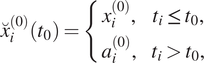
can be created that is composed of the true observation $ {x}_i^{(0)} $
for past time steps and a climatological estimate
$ {x}_i^{(0)} $
for past time steps and a climatological estimate
 $$ {a}_i^{(0)}={\overline{x}}_{\mathrm{month}}^{(0)}\left({t}_i\right)+{\Delta}_{\mathrm{hour}}^{(0)}\left({t}_i\right) $$
for future values. The composite time series
![]() is always a function of the current observation time
is always a function of the current observation time $ {t}_0 $
. The climatological estimate is derived from a monthly mean value
$ {t}_0 $
. The climatological estimate is derived from a monthly mean value $ {\overline{x}}_{\mathrm{month}}^{(0)}\left({t}_i\right) $
with
$ {\overline{x}}_{\mathrm{month}}^{(0)}\left({t}_i\right) $
with
 $$ {\overline{x}}_{\mathrm{month}}^{(0)}\left({t}_i\right)={f}^{(0)}\left({x}_i^{(0)}\right) $$
and a daily anomaly $ {\Delta}_{\mathrm{hour}}^{(0)}\left({t}_i\right) $
of it with
$ {\Delta}_{\mathrm{hour}}^{(0)}\left({t}_i\right) $
of it with
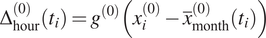 $$ {\Delta}_{\mathrm{hour}}^{(0)}\left({t}_i\right)={g}^{(0)}\left({x}_i^{(0)}-{\overline{x}}_{\mathrm{month}}^{(0)}\left({t}_i\right)\right) $$
that may vary over the year. $ {f}^{(0)} $
and
$ {f}^{(0)} $
and $ {g}^{(0)} $
are arbitrary functions used to calculate these estimates. The composite time series
$ {g}^{(0)} $
are arbitrary functions used to calculate these estimates. The composite time series
![]() can then be convolved with an FIR filter with given properties
can then be convolved with an FIR filter with given properties $ {b}_i^{(0)} $
. The result of this convolution is a low-pass filtered time series:
$ {b}_i^{(0)} $
. The result of this convolution is a low-pass filtered time series:
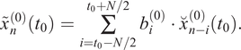
It should be noted again that $ {\tilde{x}}_i^{(0)} $
is still a function of the current observation time
$ {\tilde{x}}_i^{(0)} $
is still a function of the current observation time $ {t}_0 $
. From the composite time series and its filtered result, a residual
$ {t}_0 $
. From the composite time series and its filtered result, a residual
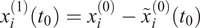 $$ {x}_i^{(1)}\left({t}_0\right)={x}_i^{(0)}-{\tilde{x}}_i^{(0)}\left({t}_0\right) $$
can be calculated, which represents the equivalent high-pass signal.
A new filtering step can now be applied to the residual $ {x}_i^{(1)}\left({t}_0\right) $
. For this, the a priori information, which is used to estimate the future, is first newly calculated. Ideally, if the first filter application in equation (5) has already completely removed the seasonal cycle, the climatological mean
$ {x}_i^{(1)}\left({t}_0\right) $
. For this, the a priori information, which is used to estimate the future, is first newly calculated. Ideally, if the first filter application in equation (5) has already completely removed the seasonal cycle, the climatological mean $ {\overline{x}}_{\mathrm{month}}^{(1)}\left({t}_i\right) $
is zero, and based on our assumption in equation (2), only an estimate of the hourly daily anomaly
$ {\overline{x}}_{\mathrm{month}}^{(1)}\left({t}_i\right) $
is zero, and based on our assumption in equation (2), only an estimate of the hourly daily anomaly $ {\Delta}_{\mathrm{hour}}^{(1)}\left({t}_i\right) $
remains. With this information, a composite time series
$ {\Delta}_{\mathrm{hour}}^{(1)}\left({t}_i\right) $
remains. With this information, a composite time series
![]() can now be formed, which can separate higher frequency oscillation components using another low-pass filter with a higher cutoff frequency. A time series
can now be formed, which can separate higher frequency oscillation components using another low-pass filter with a higher cutoff frequency. A time series $ {\tilde{x}}_n^{(1)}\left({t}_0\right) $
created in this way corresponds to the application of a band-pass filter. On the residual
$ {\tilde{x}}_n^{(1)}\left({t}_0\right) $
created in this way corresponds to the application of a band-pass filter. On the residual $ {x}_i^{(2)}\left({t}_0\right) $
, the next filter iteration with corresponding a priori information can be carried out. Generalized, equations (1)–(6) result in
$ {x}_i^{(2)}\left({t}_0\right) $
, the next filter iteration with corresponding a priori information can be carried out. Generalized, equations (1)–(6) result in
 $$ \hskip-8.3em {\overline{x}}_{\mathrm{month}}^{(j)}\left({t}_i\right)={f}^{(j)}\left({x}_i^{(j)}\right), $$
 $$ {\Delta}_{\mathrm{hour}}^{(j)}\left({t}_i\right)={g}^{(j)}\left({x}_i^{(j)}-{\overline{x}}_{\mathrm{month}}^{(j)}\left({t}_i\right)\right), $$
 $$ \hskip2.6em {a}_i^{(j)}={\overline{x}}_{\mathrm{month}}^{(j)}\left({t}_i\right)+{\Delta}_{\mathrm{hour}}^{(j)}\left({t}_i\right), $$
 $$ \hskip-3.95em {x}_i^{\left(j+1\right)}\left({t}_0\right)={x}_i^{(j)}-{\tilde{x}}_i^{(j)}\left({t}_0\right). $$
If a time series was decomposed according to this procedure using equations (7)–(12) with $ J $
filters, it now consists of a component
$ J $
filters, it now consists of a component $ {\tilde{x}}^{(0)} $
, that contains all low-frequency components,
$ {\tilde{x}}^{(0)} $
, that contains all low-frequency components, $ J-1 $
components
$ J-1 $
components $ {\tilde{x}}^{(j)} $
with oscillations on different frequency intervals, and a residual term
$ {\tilde{x}}^{(j)} $
with oscillations on different frequency intervals, and a residual term $ {x}^{(J)} $
that only covers the high-frequency components. The original signal can be completely reconstructed at any time
$ {x}^{(J)} $
that only covers the high-frequency components. The original signal can be completely reconstructed at any time $ {t}_i $
by summing up the individual components.
$ {t}_i $
by summing up the individual components.
In this study, oscillation patterns that have a periodicity of months or years are separated from the series in the first filter iteration by using a cutoff period of 21 days, which is motivated by the work of Kang et al. (Reference Kang, Hogrefe, Foley, Napelenok, Mathur and Rao2013). We also consider a cutoff period of around 75 days, as used, for example, in Rao et al. (Reference Rao, Zurbenko, Neagu, Porter, Ku and Henry1997) and Wise and Comrie (Reference Wise and Comrie2005), and evaluate the impact of this low-frequency cutoff. For the further decomposition of the time series, we first follow the cutoff frequencies proposed in Kang et al. (Reference Kang, Hogrefe, Foley, Napelenok, Mathur and Rao2013) and divide the time series into the four components baseline (BL, period >21 days), synoptic (SY, period >2.7 days), diurnal (DU, period >11 hr), and intraday (ID, residuum). Since Kang et al. (Reference Kang, Hogrefe, Foley, Napelenok, Mathur and Rao2013) found that a clear separation of the individual components is not possible for the short-term components, but can be achieved between the long-term and short-term components, we conduct a second series of experiments in which the input data are only divided into long term (LT, period >21 days) and short term (ST, residuum).
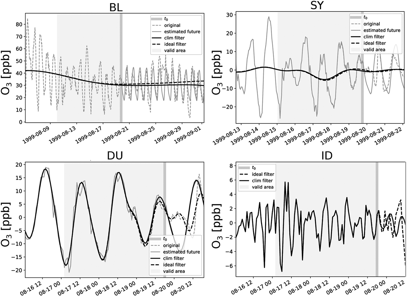
Figure 1 shows the result of such a decomposition into four components. It can be seen that the BL component decreases with time. The SY component fluctuates around zero with a moderate oscillation between August 16 and 20. In the DU component, the day-to-day variability and diurnal oscillation patterns are visible, and in the ID series, several positive and negative peaks are apparent. Overall, it can be seen that the climatological statistical estimation of the future provides a reliable prediction. However, since a slightly higher ozone episode from August 25 onward cannot be covered by the climatology, the long-term component BL is slightly underestimated, but for time points up to $ {t}_0 $
, this has hardly any effect. This small difference of a few parts per billion (ppb) is covered by the SY and DU components, so that the residual component ID no longer contains any deviations.
$ {t}_0 $
, this has hardly any effect. This small difference of a few parts per billion (ppb) is covered by the SY and DU components, so that the residual component ID no longer contains any deviations.
Decomposition of an ozone time series into baseline (BL), synoptic (SY), diurnal (DU), and intraday (ID) components at $ {t}_0= $
August 19, 1999 (dark gray background) at an arbitrary sample site (here DEMV004). Shown are the true observations
$ {t}_0= $
August 19, 1999 (dark gray background) at an arbitrary sample site (here DEMV004). Shown are the true observations $ {x}_i^{(j)} $
(dashed light gray), the a priori estimation
$ {x}_i^{(j)} $
(dashed light gray), the a priori estimation $ {a}_i^{(j)} $
about the future (solid light gray), the filtering of the time series composed of observation and a priori information
$ {a}_i^{(j)} $
about the future (solid light gray), the filtering of the time series composed of observation and a priori information $ {\tilde{x}}_i^{(j)}\left({t}_0\right) $
(solid black), and the response of a noncausal filter with access to future values (dashed black) as a reference for a perfect filtering. Because of boundary effects, only values inside the marked area (light gray background) are valid.
$ {\tilde{x}}_i^{(j)}\left({t}_0\right) $
(solid black), and the response of a noncausal filter with access to future values (dashed black) as a reference for a perfect filtering. Because of boundary effects, only values inside the marked area (light gray background) are valid.
2.2. Multibranch NN
The time series divided into individual components according to Section 2.1 serves as the input of an MB-NN. In this work, we investigate three different types of MB-NNs based on fully connected, convolutional, or recurrent layers. We therefore refer to the corresponding NNs in the following as MB-FCN, MB-CNN, and MB-RNN. The respective filter components of all input variables are presented together to one branch each. Thereby, each filter component leads to a distinct input branch in the NN. A branch first learns the local characteristics of the oscillation patterns and can therefore also be understood as its own subnetwork. Afterward, the MB-NN can learn global links, that is, the interaction of the different scales, by a learned (nonlinear) combination of the individual branches in a subsequent network. However, the individual branches are not trained separately, but the error signal propagates from the very last layer backward through the entire network and then splits up between the individual branches.
The sample MB-NN shown on the left in Figure 2 consists of four input branches, each receiving a component from the long-term $ {\tilde{x}}^{(0)} $
(BL) to the residual
$ {\tilde{x}}^{(0)} $
(BL) to the residual $ {x}^{(3)} $
(ID) of the filter decomposition. Here, the data presented as example input are the same as in Figure 1, but each component has already been scaled to a mean of zero and a standard deviation of 1, taking into account several years of data. In addition to the characteristics of the example already discussed in Section 2.1, it can be seen from the scaling that the BL component is above the mean, indicating a slightly increased long-term ozone concentration. The SY component, on the other hand, shows only a weak fluctuation. The data are fed into four different branches, each of which consists of an arbitrary architecture based on fully connected, convolutional, or recurrent layers. Subsequently, the information of these four subnetworks is concatenated and parsed in the tail to a concluding neural block, which finally results in the output layer.
$ {x}^{(3)} $
(ID) of the filter decomposition. Here, the data presented as example input are the same as in Figure 1, but each component has already been scaled to a mean of zero and a standard deviation of 1, taking into account several years of data. In addition to the characteristics of the example already discussed in Section 2.1, it can be seen from the scaling that the BL component is above the mean, indicating a slightly increased long-term ozone concentration. The SY component, on the other hand, shows only a weak fluctuation. The data are fed into four different branches, each of which consists of an arbitrary architecture based on fully connected, convolutional, or recurrent layers. Subsequently, the information of these four subnetworks is concatenated and parsed in the tail to a concluding neural block, which finally results in the output layer.
Sketching of two arbitrary MB-NNs with inputs divided into four components (BL, SY, DU, and ID) on the left and two components (LT and ST) on the right. The input example shown here corresponds to the data shown in Figure 1, whereby the components SY, DU, and ID on the right-hand side have not been decomposed, but rather grouped together as the short-term component ST. Moreover, the data have already been scaled. Each input component of a branch consists of several variables, indicated schematically by the boxes in different shades of gray. The boxes identified by the branch name, also in gray, each represent an independent neuronal block with user-defined layer types such as fully connected, convolutional, or recurrent layers and any number of layers. Subsequently, the branches are then combined via a concatenation layer marked as “C.” This is followed by a final neural block labeled as “Tail,” which can also have any configuration and finally ends in the output layer of the NN indicated by the tag “O3.” The sketches are based on a visualization with the Net2Vis tool (Bauerle et al., Reference Bauerle, van Onzenoodt and Ropinski2021).
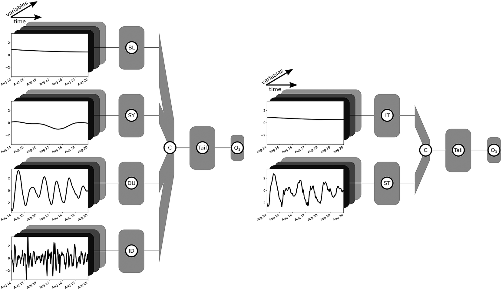
On the right side in Figure 2, only the decomposition into the two components LT and ST is applied. Since the cutoff frequency is the same for LT and BL, the LT input is equal to the BL input. All short-term components are combined and fed to the NN in the form of the ST component. This arbitrary MB-NN again uses a specified type of neural layers in each branch before the information is interconnected in the concatenate layer and then processed in the subsequent neural block, which finally leads to the output again. Figure 2 shows a generic view of the four-branch and two-branch NNs. The specific architectures employed in this study are depicted in Section 3.3, Tables B2 and B3 in Appendix B, and Figures D1– D5 in Appendix D.
3. Experiment Setup
For data preprocessing and model training and evaluation, we employ the software MLAir (version 2.0.0; Leufen et al., Reference Leufen, Kleinert, Weichselbaum, Gramlich and Schultz2022). MLAir is a tool written in Python that was developed especially for the application of ML to meteorological time series. The program executes a complete life cycle of an ML training, from preprocessing to training and evaluation. A detailed description of MLAir can be found in Leufen et al. (Reference Leufen, Kleinert and Schultz2021).
3.1. Data
In this study, data from the Tropospheric Ozone Assessment Report database (TOAR DB; Schultz et al., Reference Schultz, Schröder, Lyapina, Cooper, Galbally, Petropavlovskikh, Von Schneidemesser, Tanimoto, Elshorbany and Naja2017) are used. This database collects global in situ observation data with a special focus on air quality and in particular on ozone. As part of the Tropospheric Ozone Assessment Report (TOAR, 2021), over 10,000 air quality measuring stations worldwide were inserted into the database. For the area over Central Europe, these observations are supplemented by model reanalysis data interpolated to the measuring stations, which originate from the consortium for small-scale modeling (COSMO) reanalysis with 6-km horizontal resolution (COSMO-REA6; Bollmeyer et al., Reference Bollmeyer, Keller, Ohlwein, Wahl, Crewell, Friederichs, Hense, Keune, Kneifel, Pscheidt, Redl and Steinke2015). The measured data provided by the German Environment Agency (Umweltbundesamt) are available in hourly resolution.
By following Kleinert et al. (Reference Kleinert, Leufen and Schultz2021), we choose a set of nine input variables. As regards chemistry, we use the observation of O3 as well as the measured values of NO and NO2, which are important precursors for ozone formation. In this context, it would be desirable to include other chemical variables and especially volatile organic compounds (VOCs), such as isoprene and acetaldehyde, which have a crucial influence on the ozone production regime (Kumar and Sinha, Reference Kumar and Sinha2021). However, the measurement coverage of VOCs is very low, so that only very sporadic recordings are available, which would result in a rather small dataset. Concerning meteorology, in addition to the wind in its individual components as well as the height of the planetary boundary layer as an indicator for advection and mixing, we use temperature and the cloud cover as a proxy for solar irradiance, and the relative humidity. All meteorological variables are extracted from COSMO-REA6, but are treated in the following as if they were observations at the measuring stations. Table 1 provides an overview of the observation and model variables used. The target variable ozone is also obtained directly from the TOAR DB. Rather than using the hourly values, however, the daily aggregation to the daily maximum 8-hr average value according to the European Union definition (dma8eu) is performed by the TOAR DB and extracted directly in daily resolution. It is important to note that the calculation of dma8eu includes observations from 5 p.m. of the previous day (cf. European Parliament and Council of the European Union, 2008). Care must therefore be taken that ozone values from 5 p.m. on the day of $ {t}_0 $
may no longer be used as inputs to ensure a clear separation, as they are already included in the calculation of the target value.
$ {t}_0 $
may no longer be used as inputs to ensure a clear separation, as they are already included in the calculation of the target value.
Input and target variables with respective temporal resolution and origin. Data labeled with UBA originate from measurement sites provided by the German Environment Agency, and data with flag COSMO-REA6 have been taken from reanalysis.

Abbreviations: COSMO-REA6, consortium for small-scale modeling reanalysis with 6-km horizontal resolution; UBA, Umweltbundesamt.
This study is based on a relatively homogeneous dataset, so that the NNs can learn better and thus the effect due to time series filtering becomes clearer. In order to obtain such a dataset of observations, we restrict our investigations to the area of the North German Plain, which includes all areas in Germany north of 52.5°N. We choose this area because of the rather flat terrain; no station is located higher than 150 m above sea level. In addition, we restrict ourselves to measurement stations that are classified as background according to the European Environmental Agency AirBase classification (European Parliament and Council of the European Union, 2008), which means that no industry or major road is located in the direct proximity of the stations and consequently the pollution level of this station is not dominated by a single source. All stations are located in a rural or suburban environment. These restrictions result in a total number of 55 stations distributed over the entire area of the North German Plain. A geographical overview can be found in Figure A2 in Appendix A. It should be noted that no measuring station provides complete time series, so that gaps within the data occur. However, since the filter approach requires continuous data, gaps of up to 24 consecutive hours on the input side and gaps of 2 days on the target side are filled by linear interpolation along time.
3.2. Preparing of input and target data
The entire dataset is split along the temporal axis into training, validation, and test data. For this purpose, all data in the period from January 1, 1997 to December 31, 2007 are used for training. The a priori information of the time series filter about seasonal and diurnal cycles is calculated based on this set. The following 2 years, January 1, 2008 to December 31, 2009, are used for the validation of the training, and all data from January 1, 2010 onward are used for the final evaluation and testing of the trained model. For the meteorological data, there are no updates in the TOAR DB since January 1, 2015, so more recent air quality measurements cannot be used in this study.
For each time step $ {t}_0 $
, the time series is decomposed using the filter approach as defined in Section 2.1. The a priori information is obtained from the training dataset alone so that validation and test datasets remain truly independent. Afterward, the input variables are standardized so that each filter component of each variable has a mean of zero and a standard deviation of 1 (Z-score normalization). For the target variable dma8eu ozone, we choose the Z-score normalization as well. All transformation properties for both inputs and targets are calculated exclusively on the training data and applied to the remaining subsets. Moreover, these properties are not determined individually per station, but jointly across all measuring stations.
$ {t}_0 $
, the time series is decomposed using the filter approach as defined in Section 2.1. The a priori information is obtained from the training dataset alone so that validation and test datasets remain truly independent. Afterward, the input variables are standardized so that each filter component of each variable has a mean of zero and a standard deviation of 1 (Z-score normalization). For the target variable dma8eu ozone, we choose the Z-score normalization as well. All transformation properties for both inputs and targets are calculated exclusively on the training data and applied to the remaining subsets. Moreover, these properties are not determined individually per station, but jointly across all measuring stations.
In this work, we choose the number of past time steps for the input data as 65 hr. This corresponds to the three preceding days minus the measurements starting at 5 p.m. on the current day of $ {t}_0 $
due to the calculation procedure of dma8eu as already mentioned. The number of time steps to be predicted is set to the next 4 days for the target. All in all, we use almost 100,000 training samples and 20,000 and 30,000 samples for validation and testing, respectively (see Table 2 for exact numbers). The data availability at individual stations, as well as the total number of different stations at each point in time, is shown in Figures A1 and A3 in Appendix A, respectively. The visible larger data gaps are caused by a series of missing values that exceed the maximum interpolation length.
$ {t}_0 $
due to the calculation procedure of dma8eu as already mentioned. The number of time steps to be predicted is set to the next 4 days for the target. All in all, we use almost 100,000 training samples and 20,000 and 30,000 samples for validation and testing, respectively (see Table 2 for exact numbers). The data availability at individual stations, as well as the total number of different stations at each point in time, is shown in Figures A1 and A3 in Appendix A, respectively. The visible larger data gaps are caused by a series of missing values that exceed the maximum interpolation length.
Number of measurement stations and resulting number of samples used in this study. All stations are classified as background and situated either in a rural or suburban surrounding in the area of the North German Plain. Data are split along the temporal axes into three subsequent blocks for training, validation, and testing.

3.3. Training setup and hyperparameter search
First, we search for an optimal decomposition of the input time series for the NNs by optimizing the hyperparameters for the MB-FCN. Second, we use the most suitable decomposition and train different MB-CNNs and MB-RNNs on these data. Finally, we train equivalent network architectures without decomposition of the input time series to obtain a direct comparison of the decomposition approach as outlined in Section 3.4. All experiments are assessed based on the mean square error (MSE), as presented in Section 3.5. Since we are testing a variety of different models, we have summarized the most relevant abbreviations in Table 3.
Summary of model acronyms used in this study depending on their architecture and the number of input branches. The abbreviations for the branch types refer to the unfiltered original raw data and either to the temporal decomposition into the four components baseline (BL, period >21 days), synoptic (SY, period >2.7 days), diurnal (DU, period >11 hr), and intraday (ID, residuum), or to the decomposition into two components long term (LT, period >21 days) and short term (ST, residuum). When multiple input components are used, as indicated in the column labeled Count, the NNs are constructed with multiple input branches, each receiving a single component, and are therefore referred to as multibranch (MB). For technical reasons, this MB approach is not applicable to the OLS model, which instead uses a flattened version of the decomposed inputs and is therefore not specified as MB.
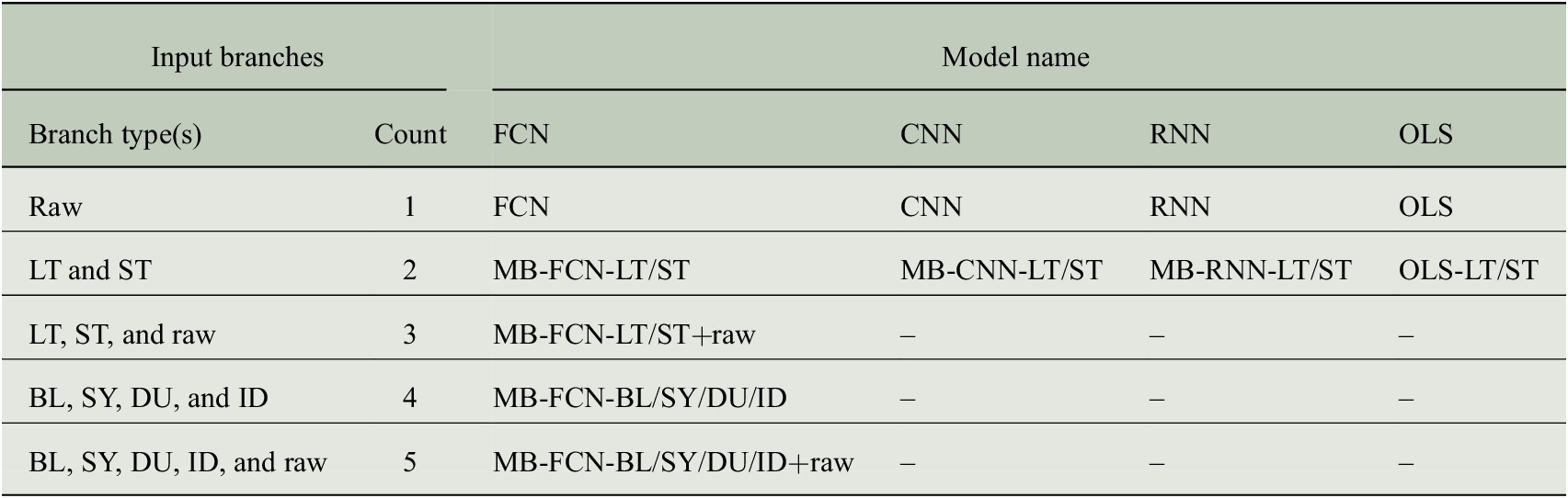
Abbreviations: CNN, convolutional neural network; FCN; fully connected network; OLS, least squares regression.
The experiments to find an optimal decomposition of the inputs and best hyperparameters for the MB-FCN start with the same cutoff frequencies for decomposition as used in Kang et al. (Reference Kang, Hogrefe, Foley, Napelenok, Mathur and Rao2013), who divide their data into the four components BL, SY, DU, and ID, as explained in Section 2.1. Since there is generally no optimal a priori choice for a filter (Oppenheim and Schafer, Reference Oppenheim and Schafer1975) and furthermore this is likely to vary from one application to another, we choose a Kaiser filter (Kaiser, Reference Kaiser, Kuo and Kaiser1966) with a beta parameter of $ \beta =5 $
for the decomposition of the time series. We prefer this filter for practical considerations, as a filter with a Kaiser window features a sharper gain reduction in the transition area at the cutoff frequency in comparison to the KZ filter. Based on this, we test a large number of combinations of the hyperparameters (see Table B1 in Appendix B for details). The trained MB-FCN with the lowest MSE on the validation in this experiment is referred to as MB-FCN-BL/SY/DU/ID in the following. Since, as already mentioned in Section 2.1, a clear decomposition in individual components is not always possible, we start a second series of experiments in which the input data are only divided into long term (LT) and short term (ST). We tested cutoff periods of 75 (Rao et al., Reference Rao, Zurbenko, Neagu, Porter, Ku and Henry1997; Wise and Comrie, Reference Wise and Comrie2005) and 21 days (Kang et al., Reference Kang, Hogrefe, Foley, Napelenok, Mathur and Rao2013), and found no difference with respect to the MSE of the trained networks. Hence, we selected the cutoff period of 21 days and refer to the trained network as MB-FCN-LT/ST in the following. After finding an optimal set of hyperparameters for both experiments, we vary the input data and study the resulting effect on the prediction skill. In two extra experiments, we add an additional branch with the unfiltered raw data to the inputs. According to the previous labels, these experiments result in the NNs labeled MB-FCN-BL/SY/DU/ID+raw and MB-FCN-LT/ST+raw. We have summarized the optimal hyperparameters for each of the MB-FCN architectures in Table B2 in Appendix B.
$ \beta =5 $
for the decomposition of the time series. We prefer this filter for practical considerations, as a filter with a Kaiser window features a sharper gain reduction in the transition area at the cutoff frequency in comparison to the KZ filter. Based on this, we test a large number of combinations of the hyperparameters (see Table B1 in Appendix B for details). The trained MB-FCN with the lowest MSE on the validation in this experiment is referred to as MB-FCN-BL/SY/DU/ID in the following. Since, as already mentioned in Section 2.1, a clear decomposition in individual components is not always possible, we start a second series of experiments in which the input data are only divided into long term (LT) and short term (ST). We tested cutoff periods of 75 (Rao et al., Reference Rao, Zurbenko, Neagu, Porter, Ku and Henry1997; Wise and Comrie, Reference Wise and Comrie2005) and 21 days (Kang et al., Reference Kang, Hogrefe, Foley, Napelenok, Mathur and Rao2013), and found no difference with respect to the MSE of the trained networks. Hence, we selected the cutoff period of 21 days and refer to the trained network as MB-FCN-LT/ST in the following. After finding an optimal set of hyperparameters for both experiments, we vary the input data and study the resulting effect on the prediction skill. In two extra experiments, we add an additional branch with the unfiltered raw data to the inputs. According to the previous labels, these experiments result in the NNs labeled MB-FCN-BL/SY/DU/ID+raw and MB-FCN-LT/ST+raw. We have summarized the optimal hyperparameters for each of the MB-FCN architectures in Table B2 in Appendix B.
Based on the findings with the MB-FCNs, we choose the best MB-FCN and the corresponding preprocessing and temporal decomposition of the input time series for the second part of the experiments, in which we test more sophisticated network architectures. With the data remaining the same, we investigate to what extent using MB-CNN or MB-RNN leads to an improvement compared to MB-FCN and also in relation to their counterparts without temporal decomposition (CNN and RNN). For this purpose, we test different architectures for CNN and RNN with and without temporal decomposition separately and compare the best representative found by the experiment, respectively. The optimal hyperparameters given by this experiments are outlined in Table B3 in Appendix B, and a visualization of the best NNs can be found in Figures D1– D5 in Appendix D. Regarding the CNN architecture, we varied the total number of layers and filters in each layer, the filter size, the use of pooling layers, as well as the application of convolutional blocks after the concatenate layer and the layout of the final dense layers. For the RNNs, during hyperparameter search, we used different numbers of LSTM cells per layer and tried stacked LSTM layers. Furthermore, we added recurrent layers after the concatenate layer in some experiments. In general, we tested different dropout rates, learning rates, a decay of the learning rate, and several activation functions.
3.4. Reference forecasts
We compare the results of the trained NNs with a persistence forecast, which generally performs well on short-term predictions (Murphy, Reference Murphy1992; Wilks, Reference Wilks2006). The persistence consists of the last observation, in this case the value of dma8eu ozone on the day of $ {t}_0 $
, which serves as a prediction for all future days. We also compare the results with climatological reference forecasts following Murphy (Reference Murphy1988). Details are given in Section 3.5. Furthermore, we compare the MB-NNs to an ordinary least squares regression (OLS), an FCN, a CNN, and an RNN. The basis for these competitors is hourly data without special preparation, that is, without prior decomposition into the individual components. The parameters of the OLS are created analogously to the NNs on the training data only. For the FCN, CNN, and RNN, sets of optimal parameters were determined experimentally in preliminary experiments also on training data. Only the NNs with the lowest MSE on the validation data are shown here. Furthermore, as with MB-NNs, we apply an OLS method to the temporally decomposed input data. For technical reasons, the OLS approach is not able to work with branched data and therefore uses flattened inputs instead. Finally, we draw a comparison with the IntelliO3-ts model from Kleinert et al. (Reference Kleinert, Leufen and Schultz2021). IntelliO3-ts is a CNN based on inception blocks (see Section 1). In contrast to the study here, IntelliO3-ts was trained for the entire area of Germany. It should be noted that IntelliO3-ts is based on daily aggregated input data, whereas all NNs trained in this study use an hourly resolution of input data. For all models, the temporal resolution of the targets is daily, so that the NNs of this study have to deal with different temporal resolutions, which does not apply for IntelliO3-ts.
$ {t}_0 $
, which serves as a prediction for all future days. We also compare the results with climatological reference forecasts following Murphy (Reference Murphy1988). Details are given in Section 3.5. Furthermore, we compare the MB-NNs to an ordinary least squares regression (OLS), an FCN, a CNN, and an RNN. The basis for these competitors is hourly data without special preparation, that is, without prior decomposition into the individual components. The parameters of the OLS are created analogously to the NNs on the training data only. For the FCN, CNN, and RNN, sets of optimal parameters were determined experimentally in preliminary experiments also on training data. Only the NNs with the lowest MSE on the validation data are shown here. Furthermore, as with MB-NNs, we apply an OLS method to the temporally decomposed input data. For technical reasons, the OLS approach is not able to work with branched data and therefore uses flattened inputs instead. Finally, we draw a comparison with the IntelliO3-ts model from Kleinert et al. (Reference Kleinert, Leufen and Schultz2021). IntelliO3-ts is a CNN based on inception blocks (see Section 1). In contrast to the study here, IntelliO3-ts was trained for the entire area of Germany. It should be noted that IntelliO3-ts is based on daily aggregated input data, whereas all NNs trained in this study use an hourly resolution of input data. For all models, the temporal resolution of the targets is daily, so that the NNs of this study have to deal with different temporal resolutions, which does not apply for IntelliO3-ts.
3.5. Evaluation methods
The evaluation of the NNs takes place exclusively on the test data that are unknown to the models. To assess the performance of the NNs, we examine both absolute and relative measures of accuracy. Accuracy measures generally represent the relationship between a prediction and the value to be predicted. Typically, for an absolute measure of the predictive quality on continuous values, the MSE is used. The MSE is a good choice as a measure because it takes into account the bias as well as the variances and the correlation between prediction and observation. To determine the uncertainty of the MSE, we choose a resampling test procedure (cf. Wilks, Reference Wilks2006). Due to the large amount of data, a bootstrap approach is suitable. Synthetic datasets are generated from the test data by repeated blockwise resampling with replacement. For each set, the error, in our case the MSE, is calculated. With a sufficiently large number of repetitions (here $ n=1,000 $
), we can access an estimate of the error uncertainty. To reduce misleading effects caused by autocorrelation, we divide the test data along the time axis into monthly blocks and draw from these instead of the individual values.
$ n=1,000 $
), we can access an estimate of the error uncertainty. To reduce misleading effects caused by autocorrelation, we divide the test data along the time axis into monthly blocks and draw from these instead of the individual values.
To compare individual models directly with each other, we derive a skill score from the MSE as a relative measure of accuracy. In this study, the skill score always consists of the MSE of the actual forecast as well as the MSE of the reference forecast and is given by
 $$ \mathrm{SS}=1-\frac{\mathrm{MSE}}{{\mathrm{MSE}}_{\mathrm{ref}}}. $$
Accordingly, a value around zero means that no improvement over a reference could be achieved. If the skill score is positive, an improvement can generally be assumed, and if it is negative, the prediction accuracy is below the reference.
For the climatological analysis of the NN, we refer to Murphy (Reference Murphy1988), who determines the climatological quality of a model by breaking down the information into four cases. In Case 1, the forecast is compared with an annual mean calculated on data that are known to the model. For this study, we consider both the training and validation data to be internal data, since the NN used these data during training and hyperparameter search. Case 2 extends a climatological consideration by differentiating into 12 individual monthly averages. Cases 3 and 4, respectively, are the corresponding transfers of the aforementioned analyses, but on test data that are unknown to the model.
Another helpful method for the verification of predictions is the consideration of the joint distribution $ p\left({y}_i,{o}_j\right) $
of prediction
$ p\left({y}_i,{o}_j\right) $
of prediction $ {y}_i $
and observation
$ {y}_i $
and observation $ {o}_j $
(Murphy and Winkler, Reference Murphy and Winkler1987). The joint distribution can be factorized to shed light on particular facets. With the calibration-refinement factorization
$ {o}_j $
(Murphy and Winkler, Reference Murphy and Winkler1987). The joint distribution can be factorized to shed light on particular facets. With the calibration-refinement factorization
 $$ p\left({y}_i,{o}_j\right)=p\left({o}_j|{y}_i\right)\cdot p\left({y}_i\right), $$
the conditional probability $ p\left({o}_j|{y}_i\right) $
and the marginal distribution of the prediction
$ p\left({o}_j|{y}_i\right) $
and the marginal distribution of the prediction $ p\left({y}_i\right) $
are considered.
$ p\left({y}_i\right) $
are considered. $ p\left({o}_j|{y}_i\right) $
provides information on the probability of each possible event
$ p\left({o}_j|{y}_i\right) $
provides information on the probability of each possible event $ {o}_j $
occurring when a value
$ {o}_j $
occurring when a value $ {y}_i $
is predicted, and thus how well the forecast is calibrated.
$ {y}_i $
is predicted, and thus how well the forecast is calibrated. $ p\left({y}_i\right) $
indicates the relative frequency of the predicted value. It is desirable to have a distribution of
$ p\left({y}_i\right) $
indicates the relative frequency of the predicted value. It is desirable to have a distribution of $ y $
with a width equal to that for
$ y $
with a width equal to that for $ o $
.
$ o $
.
3.6. Feature importance analysis
Due to the NN’s nonlinearity, the influence of individual inputs or variables on the model is not always directly obvious. Therefore, we again use a bootstrap approach to gain insight into the feature importance. In general, we remove a certain piece of information and examine the skill score in comparison to the original prediction to see whether the prediction quality of the NN decreases or increases as a result. If the skill score remains constant, this is an indication that the examined information does not provide any additional benefit for the NN. The more negative the skill score becomes in the feature importance analysis, the more likely it is that the examined variable contains important information for the NN. In the unlikely case of a positive skill score, it can be inferred that the context of this variable was learned incorrectly and thus disturbs the prediction.
For the feature importance analysis, we take a look at three different cases. First, we analyze the influence of the temporal decomposition by destroying the information of an entire input branch, for example, all low-frequent components (BL resp. LT). This yields information about the effect of the different time scales from long term to short term and the residuum. In the second step, we adopt a different perspective and look at complete variables with all temporal components (e.g., both LT and ST components of temperature). In the third step, we drive down one tier and consider each input separately to get information about whether a single input has a very strong influence on the prediction (e.g., BL component of NO2).
To break down the information for the feature importance analysis, we randomly draw the quantity to be examined from its observations. Statistically, a test variable obtained in this way is sampled from the same distribution as the original variable. However, the test variable is detached from its temporal context as well as from the context of other variables. This procedure is repeated 100 times to reduce random effects.
The feature importance analysis considers only the influence of a single quantity and no pairwise or further correlations. However, the isolated approach already provides relevant information about the feature importance. It is important to note that this analysis can only show the importance of the inputs for the trained NN and that no physical or causal relationships can be deduced from this kind of analysis in general.
4. Results
Since a comparison of all models against each other would quickly become incomprehensible, we first look at the results of the resampling in order to obtain a ranking of MB-FCNs (see Table 3 for a summary of model acronyms). The results of the bootstrapping are shown in Figure 3 and listed also in Table C1 in Appendix C. With a block length of 1 month and 1,000 repetitions of the bootstrapping, it can be seen that the simple FCN cannot adequately represent the relationships between inputs and targets in comparison to the other models. Moreover, it is visible that the performance of the MB-FCN-BL/SY/DU/ID falls behind in comparison to the other MB-FCNs with an average $ \mathrm{MSE}>70\hskip0.22em {\mathrm{ppb}}^2 $
. The smallest resampling errors could be achieved with the models MB-FCN-BL/SY/DU/ID+raw, MB-FCN-LT/ST, and MB-FCN-LT/ST+raw.
$ \mathrm{MSE}>70\hskip0.22em {\mathrm{ppb}}^2 $
. The smallest resampling errors could be achieved with the models MB-FCN-BL/SY/DU/ID+raw, MB-FCN-LT/ST, and MB-FCN-LT/ST+raw.
Results of the uncertainty estimation of the MSE using a bootstrap approach represented as box-and-whiskers. For each model, the median is shown as a black vertical line, the mean as a green triangle, the upper and lower quartiles in the form of the box, the upper and lower whiskers, which correspond to 1.5 times the interquartile range, and outliers beyond the whiskers as individual data points. The models are ordered from top to bottom with ascending average MSE. A total of 1,000 bootstrap samples were created by resampling with the replacement of single-month blocks.
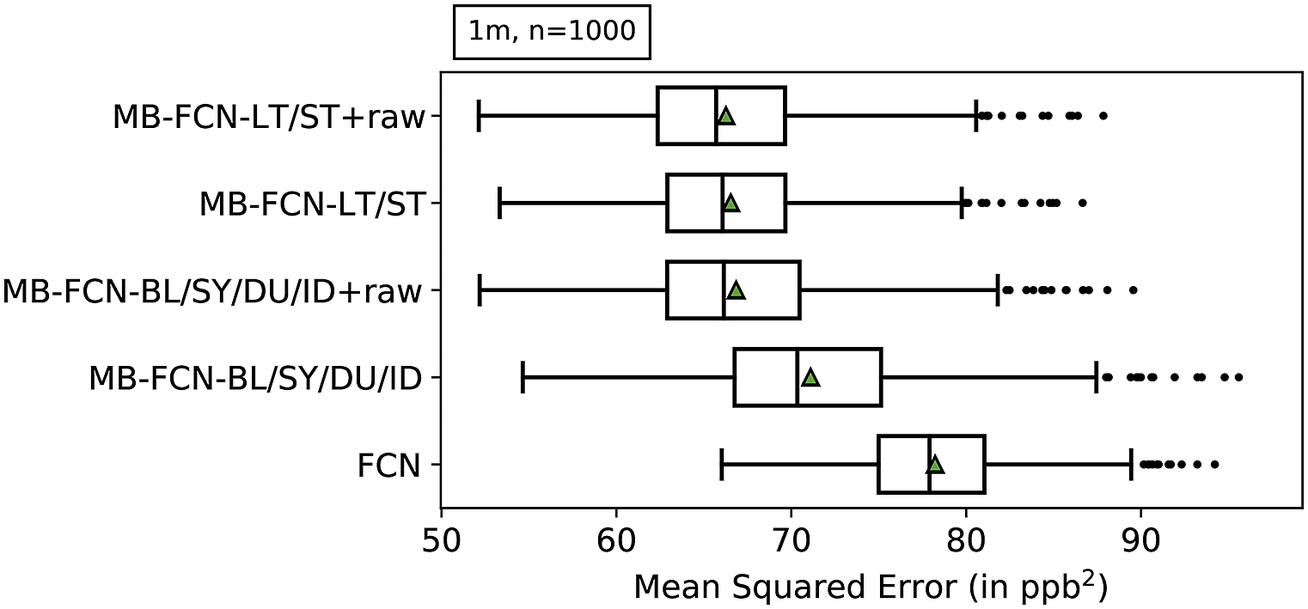
When comparing the decomposition into BL/SY/DU/ID and the decomposition into LT/ST components, the latter decomposition tends to yield a lower error. Alternatively, it is possible to achieve comparative performance by adding the raw data to both variants of decomposition. For the LT/ST decomposition, however, this improvement is marginal.
Since the forecast accuracy of the top three NNs is nearly indistinguishable, especially for the two models with the LT/ST split, we choose the MB-FCN-LT/ST network and so the LT/ST decomposition for further analysis, since, of the three winning candidates, this is the network with the smallest number of trainable parameters (see Table B2 in Appendix B).
So far, we have shown the advantages of an LT/ST decomposition during preprocessing for FCNs. Therefore, in the following, we apply our proposed decomposition to more elaborated network architectures, namely a CNN and an RNN architecture. We again consider the uncertainty estimation of the MSE using the bootstrap approach and calculate the skill score with respect to the MSE in pairs for an NN type that was trained once as an MB-NN with temporally decomposed inputs and once with the raw hourly data. Similarly, we consider the skill score of OLS on decomposed and raw data, respectively. The results are shown in Figure 4. It can be seen that the skill score is always positive for all models. This in turn means that using our proposed time decomposition of the input time series improves all the models analyzed here. When looking at the individual models, it can be differentiated that the FCN architecture in particular benefits from the decomposition, whereas the improvement is smaller for RNN and smallest but still significant for OLS and CNN.
Pairwise comparison of different models running with temporal decomposed or raw data by calculating the skill score on the results from the uncertainty estimation of the mean square error using a bootstrap approach represented as box-and-whiskers. For each model, the median is shown as a black vertical line, the mean as a green triangle, the upper and lower quartiles in the form of the box, the upper and lower whiskers, which correspond to 1.5 times the interquartile range, and outliers beyond the whiskers as individual data points. A total of 1,000 bootstrap samples were created by resampling with the replacement of single-month blocks.

Based on the uncertainty estimation of the MSE shown in Figure 5 and also listed in Table C2 in Appendix C, the models can be roughly divided into three groups according to their average MSE. The last group consists solely of the persistence prediction, which delivers a significantly worse prediction than all other methods and lies at an MSE of 107 $ {\mathrm{ppb}}^2 $
on average. In the intermediate group with an MSE between 70 and 80
$ {\mathrm{ppb}}^2 $
on average. In the intermediate group with an MSE between 70 and 80 $ {\mathrm{ppb}}^2 $
, only approaches that do not use temporally decomposed inputs are found, including the IntelliO3-ts-v1 model. Overall, the FCN performs worst with a mean MSE of 78
$ {\mathrm{ppb}}^2 $
, only approaches that do not use temporally decomposed inputs are found, including the IntelliO3-ts-v1 model. Overall, the FCN performs worst with a mean MSE of 78 $ {\mathrm{ppb}}^2 $
, and the best results in this group are achieved with the CNN. In the leading group are exclusively methods that rely on the decomposition of the input time series. The OLS with the LT/ST decomposition has the highest error within this group with 68
$ {\mathrm{ppb}}^2 $
, and the best results in this group are achieved with the CNN. In the leading group are exclusively methods that rely on the decomposition of the input time series. The OLS with the LT/ST decomposition has the highest error within this group with 68 $ {\mathrm{ppb}}^2 $
. The lowest errors can be obtained with the MB-FCN and the MB-RNN, whereby the MSE for both NNs is around 66
$ {\mathrm{ppb}}^2 $
. The lowest errors can be obtained with the MB-FCN and the MB-RNN, whereby the MSE for both NNs is around 66 $ {\mathrm{ppb}}^2 $
.
$ {\mathrm{ppb}}^2 $
.
The same as Figure 3, but for a different set of models. Results of the uncertainty estimation of the MSE using a bootstrap approach represented as box-and-whiskers. For each model, the median is shown as a black vertical line, the mean as a green triangle, the upper and lower quartiles in the form of the box, the upper and lower whiskers, which correspond to 1.5 times the interquartile range, and outliers beyond the whiskers as individual data points. The models are ordered from top to bottom with ascending average MSE. A total of 1,000 bootstrap samples were created by resampling with the replacement of single-month blocks. Note that the uncertainty estimation shown here is independent of the results shown in Figure 3, and therefore numbers may vary for statistical reasons.

In order to understand why the decomposition consistently brings about an improvement for all methods considered here, we look exemplarily at the MB-FCN-LT/ST in more detail in the following. However, it should be mentioned that the discussed aspects are also basically valid for the other NN types.
First, we have a look at the calibration-refinement factorization of the joint distribution (Figure 6) according to equation (14). It can be seen that the distribution of the forecasted concentration of ozone becomes narrower toward the mean with increasing lead time. While the MB-FCN-LT/ST is still able to predict values of >70 ppb for the 1-day forecast, it is limited to values below 60 ppb for the 4-day forecast and tends to underestimate larger concentrations with increasing lead time. According to the conditional probability of observing an issued forecast, the MB-FCN-LT/ST is best calibrated for the first forecast day and especially in the value range from 20 to 60 ppb. However, observations of high ozone concentrations, starting from values above 60 ppb, are generally underestimated by the NN. Coupled with the already mentioned narrowing of the forecast’s distribution, the underestimation of high ozone concentrations increases with lead time.
Joint distribution of prediction and observation in the calibration-refinement factorization $ p\left({y}_i,{o}_j\right) $
for the MB-FCN-LT/ST for all four lead times. On the one hand, the marginal distribution
$ p\left({y}_i,{o}_j\right) $
for the MB-FCN-LT/ST for all four lead times. On the one hand, the marginal distribution $ p\left({y}_i\right) $
of the prediction is shown as a histogram in gray colors with the axis on the right, and on the other hand, the conditional probability
$ p\left({y}_i\right) $
of the prediction is shown as a histogram in gray colors with the axis on the right, and on the other hand, the conditional probability $ p\left({o}_j|{y}_i\right) $
is expressed by quantiles in the form of differently dashed lines. The reference line of a perfectly calibrated forecast is also shown as a solid line.
$ p\left({o}_j|{y}_i\right) $
is expressed by quantiles in the form of differently dashed lines. The reference line of a perfectly calibrated forecast is also shown as a solid line.

The shortcomings with the prediction of the tails of the distribution of observations are also evident when looking at the seasonal behavior of the MB-FCN-LT/ST. Figure 7 summarizes the distribution of observations and predictions of the NN for each month. The narrowing toward the mean with increasing lead time is also clearly visible here in the whiskers and the interquartile range in the form of the box. However, it can already be observed that, from a climatological perspective, the forecasts are in the range of the observations, and the annual cycle of the ozone concentration can be modeled. Yet the month of July stands out in particular, where it is clearly recognizable that the NN is not able to represent the large variability of values from 20 ppb to values over 100 ppb that occur during summer.
Overview of the climatological behavior of the MB-FCN-LT/ST forecast shown as a monthly distribution of the observation and forecasts on the left and the analysis of the climatological skill score according to Murphy (Reference Murphy1988) differentiated into four cases on the right. The observations are highlighted in green and the forecasts in blue. As in Figure 3, the data are presented as box-and-whiskers, with the black triangle representing the mean.
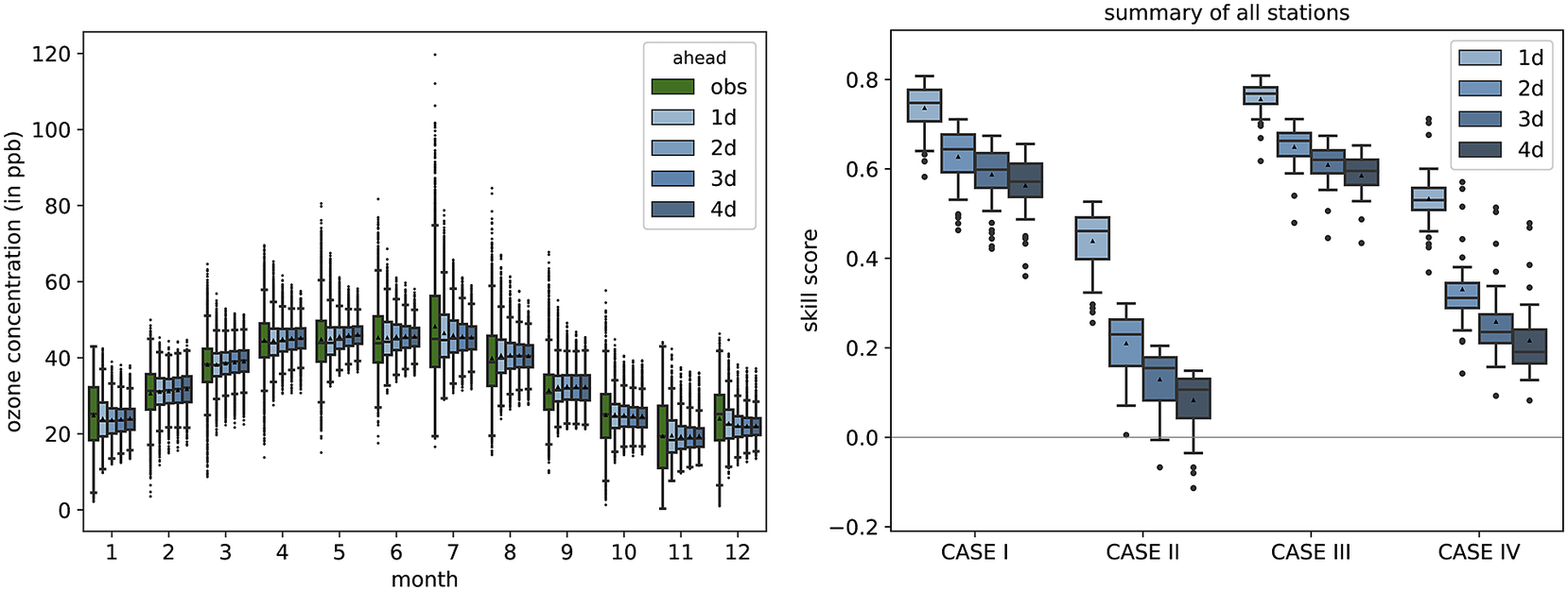
The direct comparison according to Murphy (Reference Murphy1988) between the climatological annual mean of the observation and the forecast of the NN for the training and validation data (Case 1) as well as for the test data (Case 3) shows a high skill score in favor of the NN compared to the single-valued climatological reference as the NN captures the seasonal cycle (Figure 7). Furthermore, in direct comparison with the climatological monthly means (Cases 2 and 4), the MB-FCN-LT/ST can achieve an added value in terms of information. However, the skill score on all datasets decreases gradually with longer lead times. Nonetheless, a nearly continuously positive skill score shows that the seasonal pattern of the observations can be simulated by the NN.
The feature importance analysis provides insight on which variables the MB-FCN-LT/ST generally relies upon. An examination of the importance of the individual branches, as shown in Figure 8, shows that, for the first forecast day, both LT and ST have a significant influence on the forecast accuracy. For longer forecast horizons, this influence decreases visibly, especially for ST. It is worth noting here that the influence of LT decreases less for Days 2–4, remaining at an almost constant level. Consequently, the long-term components of the decomposed time series have an important influence on all forecasts.
Importance of single branches (left) and single variables (right) for the MB-FCN-LT/ST using bootstrapping. In blue colors, the skill score for lead times from 1 day (light blue) to 4 days (dark blue) is shown. A negative skill score indicates a strong influence on the forecast performance. The skill score is calculated with the original undisturbed prediction of the same NN as reference. Note that due to the significantly stronger dependence, ozone is visualized on a separate scale.

Looking at the importance of each variable with its components shows first of all that the NN is strongly dependent on the input ozone concentration. This dependence decreases continuously with lead time. Important meteorological drivers are temperature, relative humidity, and planetary boundary layer height. All these variables diminish in importance with increasing forecast horizon, analogously to the importance of the ozone concentration. On the chemical side, NO2 also has an influence. Here, it must be emphasized that, in contrast to the other variables, the influence does not decrease with lead time, but remains constant over all forecast days. From the feature importance, we can see that the trained model does not make extensive use of information from wind, NO, or cloud cover.
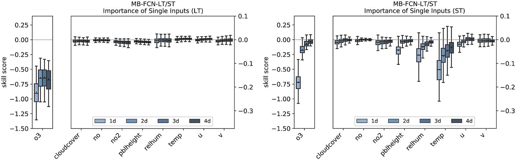
Isolating the effects of the individual inputs in the LT branch shows that the NN is hardly dependent on the long-term components of the input variables apart from ozone (see Figure 9). The importance of ozone is higher on Day 1 than on the following days, but then remains at a constant level. For the short-term components, the concentration of ozone is also decisive. However, its influence decreases rapidly from the 1-day to the 2-day forecast. The individual importance of the ST components of the other input variables behaves in the same way as the overall importance of these variables.
Importance of single inputs for the LT branch (left) and the ST branch (right) for the MB-FCN-LT/ST using a bootstrap approach. In blue colors, the skill score for lead times from 1 day (light blue) to 4 days (dark blue) is shown. A negative skill score indicates a dependence. The skill score is calculated with the original undisturbed prediction of the same NN as reference.
As previously mentioned, the points discussed before can be more or less transferred to the other NN architectures. The feature importance analysis of the branches and the individual variables for MB-CNN and MB-RNN is shown in Figures E1– E3 in Appendix E. In particular, the LT for all forecast days and the ST for the first day contain important information, with the ST branch being less relevant for the MB-RNN. Moreover, MB-CNN and MB-RNN also show a narrowing of the distribution of issued forecasts with increasing lead time, as was also observed for MB-FCN.
5. Discussion
The experimental results described in the previous section indicate that the NNs learn oscillation patterns on different time scales, and in particular climatological properties, better when the input time series are explicitly decomposed into different temporal components. The MB-NNs outperform all reference models, such as simple statistical regression methods as well as the naïve persistence forecasts and climatological references. The MB-NNs are also preferable to their corresponding counterparts without temporal decomposition, considered individually but also as a collective.
The uncertainty estimate of the MSE of the forecast shows that FCNs that either use a decomposition into a long-term and a short-term component or access unfiltered raw data as a supplementary source of information have the highest forecast accuracy. Separating the input signals into more than two components without adding the unfiltered raw data cannot improve the performance of the FCNs, with respect to the architectures chosen in this study. This recognition coincides with the findings of Kang et al. (Reference Kang, Hogrefe, Foley, Napelenok, Mathur and Rao2013), who show that a clear separation of the short-term components is generally not possible due to the superposition of multiple oscillation patterns.
With regard to the network architecture, several key points can be identified in this study. Without special processing of the input data, the best results were achieved with a CNN architecture. This could be explained by the fact that the convolutional layers of the CNN already filter the time series. However, it must also be mentioned that with a filter size of only 5 hr, there is no chance to extract an annual cycle, so that the explicit decomposition into LT and ST components also offers added value for the CNN. However, due to the higher baseline level, the MB-CNN cannot benefit as much from the data processing compared to the MB-FCN and MB-RNN and is moreover behind the other two MB-NNs in terms of prediction quality in absolute terms. The RNN also achieves better results on the unfiltered data than the FCN, for example, because it can benefit from a more specific understanding of time. The FCN is therefore inferior to the CNN and RNN due to its comparatively simple architecture and the lack of possibility to relate neighboring data points explicitly. However, it benefits most from the temporal decomposition of the inputs, so that these disadvantages disappear, and overall, the smallest errors can be achieved with MB-FCN and MB-RNN. These finding therefore highlight the importance of jointly optimizing data preprocessing and NN model architecture, which is taught in many ML courses, but not always followed in practical applications.
The difficulties of NNs to recognize annual patterns in daily resolved data noted by Cho et al. (Reference Cho, Van Merriënboer, Bahdanau and Bengio2014) did not apply to the MB-NNs. However, the networks still encounter difficulties in anticipating very low and very high ozone concentrations. As the lead time increases, the NN’s forecast strategy becomes more cautious about extremes, leading to a narrowing of the distribution of issued forecasts. Despite this circumstance, the NNs always retain within an optimal range from a climatological point of view, so that the forecast has higher accuracy than a climatological forecast. The analysis of the feature importance can provide an explanation for this. For the first day of the forecast, both long-term and short-term components have an equally strong influence on the MB-FCN forecast, but for a longer forecast horizon, the long-term components are given more weight. Accordingly, the LT branch in particular enables the NN to generate a climatologically meaningful forecast. In addition, the NN remains strongly dependent on the ozone concentrations from the inputs. Learning a form of autocorrelation is advantageous for climatological accuracy, but at the same time leads to a poorer representation of scarcer events such as sudden and strong increases in the daily maximum concentration from one day to the next.
In addition, it must be mentioned that strong deviations from climatological norm states also have an impact on the filter decomposition of the inputs, since climatology can only be an estimate of a long-term mean state, which can deviate strongly from the actual weather in individual cases. For example, the long-term signal of temperature in the case of a very warm summer would be weakened by the added climatology, since such a deviation represents an exceptional case from a climatological point of view. In this case, the second filter component, which should actually be free of an annual variation, also contains a proportion of an annual oscillation. However, as discussed in Section 2, this combination allows to apply noncausal filters in a forecasting situation, where generally only causal filters are applicable, which lead to phase shifts in the data and show larger errors.
A look at the importance of the individual inputs for the MB-FCN yields two views. First, it becomes apparent that the dependency of the LT and ST components are each strongly based on the corresponding component of the ozone concentration and that the MB-FCN accordingly learns the connection between observed hourly ozone values and the target ozone statistic. Second, all other variables seem to have an influence only on the short-term scale. Since the ST component by definition represents the deviation from the climatological normal state, it can be seen that the MB-FCN relies on the deviation from normal states as a forecasting strategy.
Finally, we would like to discuss the filters used for the decomposition. Since there are many different types of filters with various advantages and disadvantages, we have limited this work to the use of a Kaiser window and have not carried out any further experiments with different types of filters, such as the KZ filter, which could possibly lead to an improved separation of individual components as stated in Rao and Zurbenko (Reference Rao and Zurbenko1994) in the presence of a weather forecast. Furthermore, we have not undertaken any in-depth investigations into which separation frequencies lead to an optimal decomposition of the time series.
6. Conclusion
In this work, we explored the potential of training different NNs, namely FCN, CNN, and RNN, for dma8eu ozone forecasting using inputs decomposed into different frequency components from long term to short term with noncausal filters in order to improve the forecast accuracy of the NNs. The temporal decomposition of the inputs not only improves the different NN architectures and the linear OLS model, but also offers an overall added value for the prediction of ozone compared to all reference models using raw hourly inputs and naïve approaches based on persistence and climatology. As exemplary shown with the MB-FCN, the MB-NNs work better with a decomposition into two components compared to four and they rely on both long-term and short-term components for their prediction, with a strong dependence on past ozone observations and a decreasing importance of the short-term components with lead time. In order to realize a valid decomposition in a forecast setup without time delay of the signal introduced by the filter itself, a combination of observations and a priori information in the form of climatology was chosen.
Acknowledgements
The authors gratefully acknowledge the Jülich Supercomputing Centre for providing the infrastructure and resources to run all experiments. We are also thankful to all air quality data providers that made their data available in the TOAR DB.
Author Contributions
Conceptualization: All authors; Data curation: L.H.L. and F.K.; Formal analysis: L.H.L.; Funding acquisition: M.G.S.; Investigation: L.H.L.; Methodology: L.H.L.; Project administration: M.G.S.; Resources: M.G.S.; Software: L.H.L. and F.K.; Supervision: M.G.S.; Validation: All authors; Visualization: L.H.L. and F.K.; Writing—original draft: L.H.L.; Writing—review and editing: All authors.
Data Availability Statement
Replication data and code can be found on b2share: https://doi.org/10.34730/decca0f4bbfc42c693812f7a648b2d6f.
Funding Statement
This research was supported by grants from the European Research Council, H2020 Research Infrastructures (Grant No. 787576 [IntelliAQ]).
Ethical Standards
The research meets all ethical guidelines, including adherence to the legal requirements of the study country.
Competing Interests
The authors declare none.
Appendix A: Details on Data
Graphical representation of the number of samples available for training (orange), validation (green), and testing (blue) per time step. Apart from three periods in which the data cannot meet the requirements, more than 20 stations are available at each time step, and for training in particular, more than 30 stations for the most time. The graph does not show the available raw data, but indicates for which time steps $ {t}_0 $
a sample with fully processed input and target values is available.
$ {t}_0 $
a sample with fully processed input and target values is available.
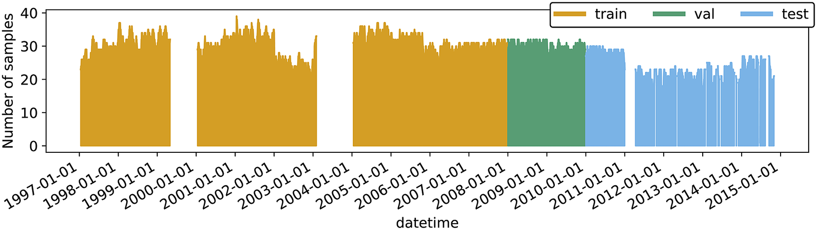
Geographical location of all rural and suburban monitoring stations used in this study divided into training (orange), validation (green), and test (blue) data represented by triangles in the corresponding colors. The tip of the triangles points to the exact location of the station.

Detailed overview of the availability of station data broken down for all individual stations as a timeline separated by color for training (orange), validation (green), and test (blue) data. Individual gaps are caused by missing observation data that exceed the interpolation limit of 24 hr for inputs or 2 days for targets.
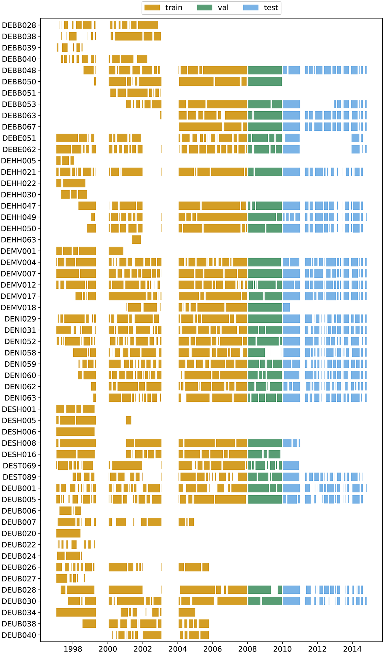
Appendix B: Details on Hyperparameter Search
Details on tested hyperparameters for the MB-FCNs. The square brackets indicate a continuous parameter range, and the curly brackets indicate a fixed set of parameters. Parameter spaces covering different orders of magnitude were sampled on a logarithmic scale. For details on the activation functions, we refer to rectified linear unit (ReLU) and leaky rectified linear unit (LeakyReLU, Maas et al., Reference Maas, Hannun and Ng2013), exponential linear unit (ELU, Clevert et al., Reference Clevert, Unterthiner and Hochreiter2016), scaled exponential linear unit (SELU, Klambauer et al., Reference Klambauer, Unterthiner, Mayr and Hochreiter2017), and parametric rectified linear unit (PReLU, He et al., Reference He, Zhang, Ren and Sun2015).
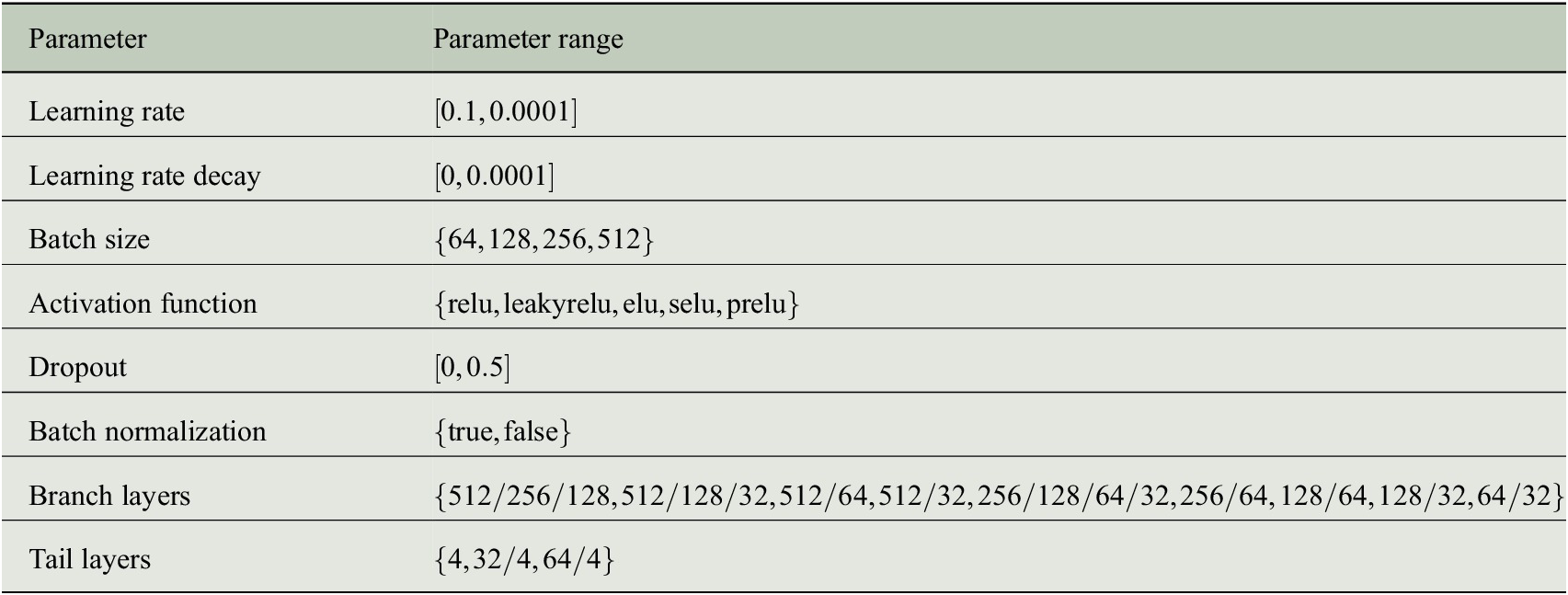
Summary of best hyperparameters and fixed parameters for different setups with MB-FCN. The entire parameter ranges of all hyperparameters are given in Table B1. Details on the activation functions can be found in He et al. (Reference He, Zhang, Ren and Sun2015) for the parametric rectified linear unit (PReLU) and in Clevert et al. (Reference Clevert, Unterthiner and Hochreiter2016) for the exponential linear unit (ELU). A visualization of MB-FCN-LT/ST can be found in Figure D1 in addition.

Abbreviation: FCN, fully connected network.
Summary of best hyperparameters and fixed parameters for experiments with the CNN, MB-CNN, RNN, and MB-RNN. The entire parameter ranges of all hyperparameters are not listed. Details on the activation functions can be found in Maas et al. (Reference Maas, Hannun and Ng2013) for the rectified linear unit (ReLU) and the leaky rectified linear unit (LeakyReLU) and in He et al. (Reference He, Zhang, Ren and Sun2015) for the parametric rectified linear unit (PReLU).
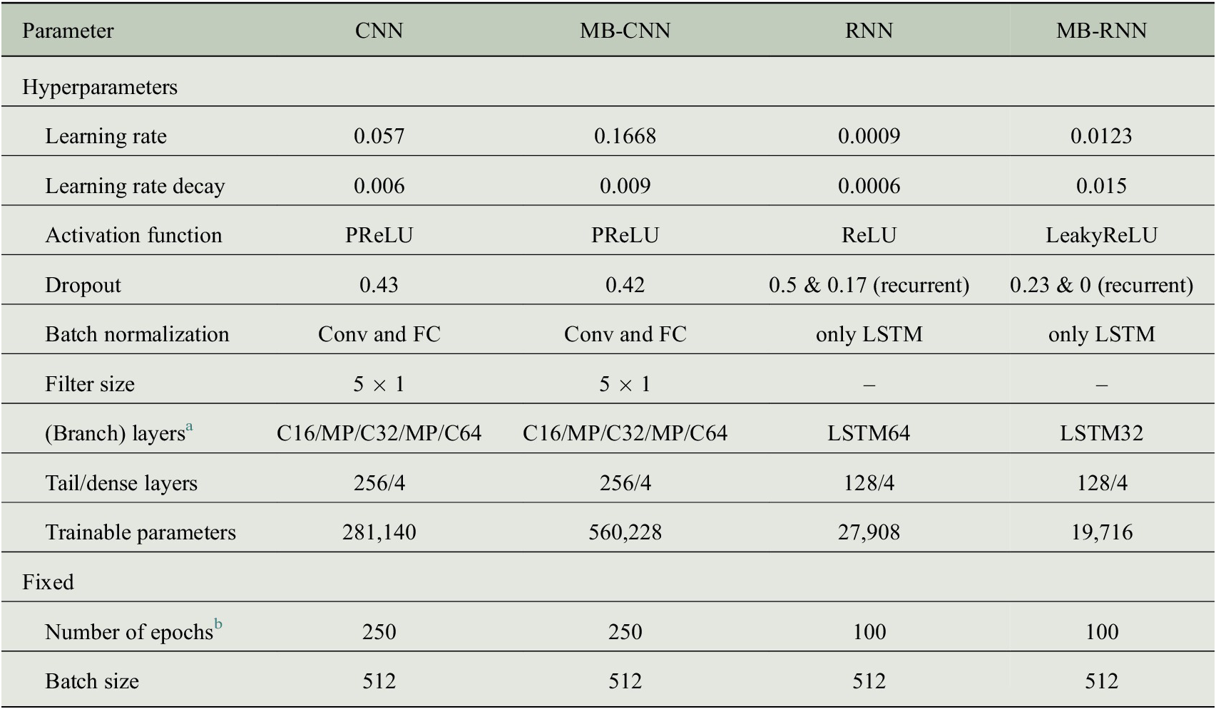
Abbreviations: CNN, convolutional neural network; LSTM, long short-term memory.
Appendix C: Tabular Results
Key numbers of the uncertainty estimation of the MSE for all MB-FCNs as an average over all prediction days using the bootstrap approach visualized in Figure 3. All reported numbers are in the unit of square parts per billion. Numbers in percentage point to the corresponding percentile of the error distribution.
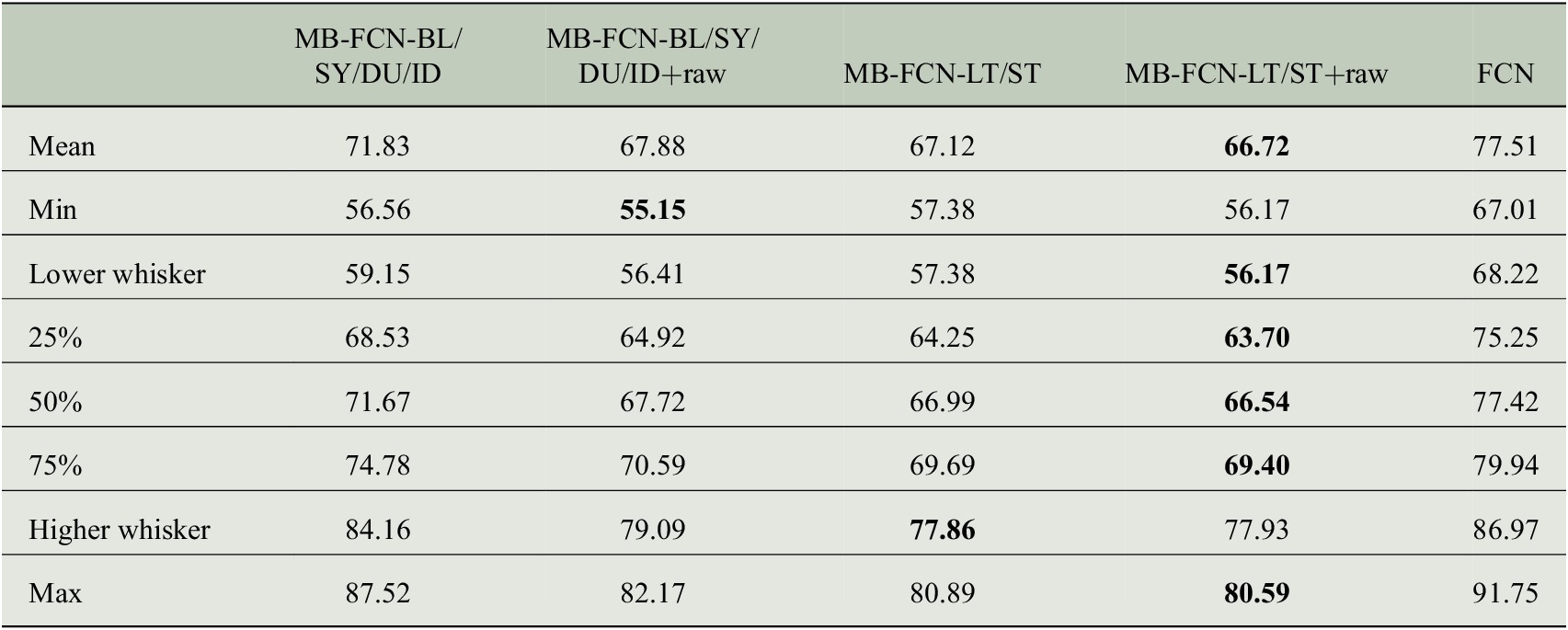
Abbreviations: FCN, fully connected network; MSE, mean square error.
Key numbers of the uncertainty estimation of the MSE as an average over all prediction days using the bootstrap approach visualized in Figure 5. All reported numbers are in the unit of square parts per billion. Numbers in percentage point to the corresponding percentile of the error distribution. Note that the uncertainty estimation reported here is independent of the results shown in Table C1, and therefore numbers may vary for statistical reasons.

Abbreviations: CNN, convolutional neural network; FCN, fully connected network; MSE, mean square error; OLS, least squares regression.
Appendix D: Model Architecture
Visualization of MB-FCN-LT/ST using the tool Net2Vis (Bauerle et al., Reference Bauerle, van Onzenoodt and Ropinski2021). Shown from left to right are the input data, followed by the flattened layer and two fully connected layers (FC) with 128 and 64 neurons. In total, the neural network has two such branches, whose weights can be trained independently of each other. All branches are concatenated and bounded by the output layer with four neurons. The orange FC block consists of a fully connected layer, a batch normalization layer, and an exponential linear unit activation. The output layer contains only a fully connected layer followed by a linear activation. The dropout layers are highlighted in purple, and all other remaining layers with nontrainable parameters are shown in gray.
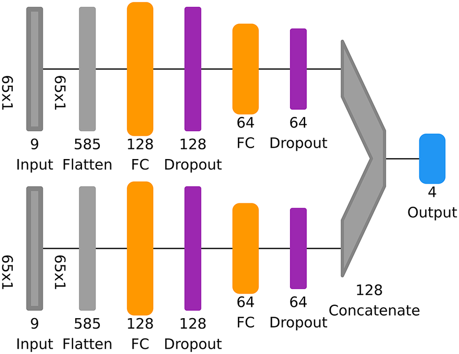
Visualization of a convolutional neural network as in Figure D1. In addition, this neural network consists of convolutional blocks highlighted in blue and MaxPooling layers shown in yellow. Each convolutional block consists of a convolutional layer with a kernel size of 5 × 1 and the same padding, followed by a batch normalization layer and a parametric rectified linear unit (PreLU) activation. The MaxPooling layers use a pooling size of 2 × 1 and strides with 2 × 1. The FC blocks in this model consist of the fully connected layer, batch normalization, and a PReLU activation.

Visualization of a multibranch convolutional neural network as in Figure D2.

Visualization of RNN as in Figure D1. In addition, the neural network shown here consists of long short-term memory layer (LSTM) blocks indicated in green. Each LSTM block includes an LSTM layer with a given number of LSTM cells within followed by a batch normalization layer and a rectified linear unit (ReLU) activation function. Note that the dropout shown here is not the recurrent dropout, but the regular dropout that is applied on the activation of a layer. The FC block also uses a ReLU activation function, but no batch normalization.

Visualization of MB-RNN as in Figure D4. Deviating here, the activation is LeakyReLU both for the long short-term memory layer and the FC layer.

Appendix E: Feature Importance of MB-CNN and MB-RNN
Importance of single branches for multibranch convolutional neural network (left) and multibranch recurrent neural network (right) as in Figure 8.
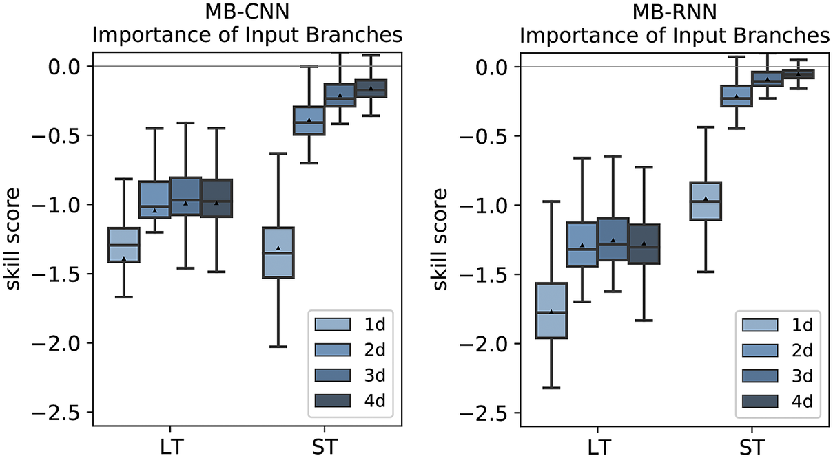
Importance of single inputs for the LT branch (left) and the ST branch (right) for the multibranch convolutional neural network.
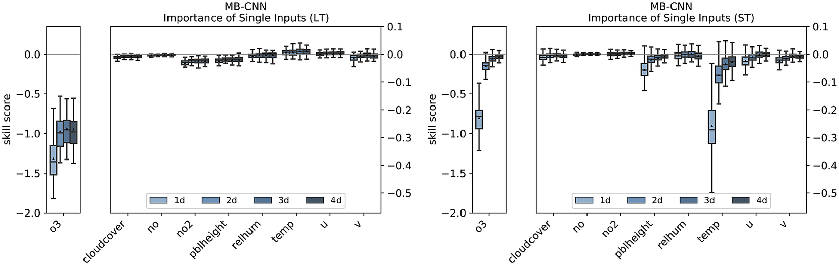
Importance of single inputs for the LT branch (left) and the ST branch (right) for the multibranch recurrent neural network.


 Open access