


1. Introduction
Over the last thirty years, microfluidic research has impacted a wide variety of fields including biology, biotechnology, physics and engineering, among others (Nunes & Stone Reference Nunes and Stone2022). Although varied in their application, all microfluidic devices are concerned with the motion of fluids at scales of the order of tens to hundreds of micrometres. At these scales traditional pressure-driven pumping mechanisms lose their efficacy and alternative ways of transporting fluids become viable. In particular, because surface area dominates over volume, numerous means of using fluid interfaces to drive flow have been suggested. These include application of electric fields to drive electrosomotic flow (Anderson Reference Anderson1989) and control leaky dielectric fluids (Melcher & Taylor Reference Melcher and Taylor1969), and the use of electric fields to induce interfacial oscillations to facilitate pumping or mixing (Cimpeanu & Papageorgiou Reference Cimpeanu and Papageorgiou2014, Reference Cimpeanu and Papageorgiou2015). Others use surface tension in the form of capillary wicking pumps such as those used in rapid COVID-19 tests (Aghajanloo et al. Reference Aghajanloo, Losereewanich, Pastras and Inglis2024). Finally, gradients of surface tension along gas–liquid interfaces are known to drive flows through the formation of viscous stresses, or Marangoni stresses, in fluids.
Marangoni stresses were first discussed by Thomson (Reference Thomson1855) who noted that the upward force responsible for the formation of tears of wine on the side of a glass was due to gradients in the surface tension in the liquid. Later this idea was discussed by Marangoni (Reference Marangoni1871), whose name is associated with the phenomenon. These gradients can be caused by any gradient in some variable that affects surface tension. For wine, which is essentially a combination of water and ethanol, higher rates of evaporation of the volatile alcohol in the thin film of wine on a glass leads to lower concentrations higher up on the glass. Surface tension is therefore largest at the top of the glass, generating a force that pulls liquid upwards, resisting gravity. A detailed experimental and theoretical study of such evaporative instabilities can be found in Hosoi & Bush (Reference Hosoi and Bush2001). Surface tension can also be affected by temperature and surfactant concentrations on gas–liquid interfaces. Both have an inverse relationship with surface tension, i.e. higher temperatures and interfacial surfactant concentrations tend to decrease surface tension. Hence, the forces generated are directed opposite field gradients and fluid will be pushed towards colder and less packed regions where the surface tension is greatest. These are sometimes referred to as thermocapillary and solutocapillary stresses to differentiate the underlying physics.
In microfluidics, both thermal and surfactant-driven Marangoni stresses have been considered as potential sources of flow control; however, they seem to excel in different roles. Thermocapillary stresses often appear as a means to pump or control fluids via some external source. For example Baier, Steffes & Hardt (Reference Baier, Steffes and Hardt2010) recognised that a superhydrophobic geometry could be transformed into a fluid pump by incorporating a temperature gradient along the length of a microfludic device. This idea was explored and verified experimentally by Amador et al. (Reference Amador, Ren, Tabak, Alapan, Yasa and Sitti2019), but flow rates were less than expected from the theory. Crowdy et al. (Reference Crowdy, Mayer and Hodes2023a ) carried out a theoretical investigation of a new design for a thermocapillary pump that uses physical asymmetry to drive fluid without requiring a macroscale temperature gradient. In another application, Miniewicz et al. (Reference Miniewicz, Bartkiewicz, Orlikowska and Dradrach2016) showed that by externally exciting a liquid film with a laser pointer, gas bubble formation and transport of that bubble through the liquid can be induced, highlighting the role of induced heat for active flow control.
On the other hand, the focus of research on surfactant-induced stresses has generally been on propulsion, that is, the self-driven motion of a floating particle. The motivation behind this is many-fold. For instance, it is an effect that occurs in nature where some species of beetles secrete surfactant to move around water surfaces (Bush & Hu Reference Bush and Hu2006). It is also of direct interest for the study of so-called Janus particles (Golestanian, Liverpool & Ajdari Reference Golestanian, Liverpool and Ajdari2005; Masoud & Stone Reference Masoud and Stone2014; Yariv & Crowdy Reference Yariv and Crowdy2020), which self-propel due to non-uniformity in surface properties. These particles directly translate chemical energy into mechanical motion, as in the self-propulsion of dissolving metals in hydrogen peroxide (Suematsu & Nakata Reference Suematsu and Nakata2018). Moreover self-propelled objects considered in a group enable better understanding of complex biological, chemical and physical systems. For example, Frenkel et al. (Reference Frenkel, Multanen, Grynyov, Musin, Bormashenko and Bormashenko2017) used camphor boats to develop so-called chemical gardens, complex tubular structures formed by a complex combination of chemical and hydrodynamic events. Along these lines, Crowdy (Reference Crowdy2021a ) used complex analysis to look at the motion of a flotilla of two-dimensional camphor boats moving at constant speed.
It is noteworthy that thermocapillary stresses seem adequate for pumping applications while surfactants are limited to particle propulsion. We conjecture that the reason for this is due to the significantly different transport properties between heat and surfactant. First, it is far easier to set up the macroscopic gradients necessary to pump using heat, accomplished by imposing a linear temperature field across the length of a channel, as done by Amador et al. (Reference Amador, Ren, Tabak, Alapan, Yasa and Sitti2019). The analogue for surfactant would require constant surfactant concentrations upstream and downstream which is difficult at steady state as the surfactant will begin to deplete from the source of higher concentration. Conversely, for particle propulsion it is advantageous for each particle to carry its fuel with it as opposed to either carrying a heating device or heating each particle externally.
Moreover, heat excels at active flow control because its larger diffusivity makes it far easier to induce rapid changes. Thermal diffusivity in water is roughly 1000 times faster than that of a typical surfactant, so it can be used as in the experiments of Miniewicz et al. (Reference Miniewicz, Bartkiewicz, Orlikowska and Dradrach2016), for example, where they heat a liquid near an interface with a laser. The heat diffuses rapidly to the interface, which sets up a thermocapillary flow that bends the interface, forms a gas bubble and traps the bubble onto the trailing edge of a moving laser pointer. There is no real analogue to this with surfactants as it would require point additions of surfactant and be severely limited by the slow transport of surfactant to the interface.
It is important, however, to study surfactants as a viable source of active interface control. One valuable characteristic is that even traces of surfactant often have extremely large effects on the surface tension of water. For example, only a $10^{-4}$
M (
$10^{-4}$
M ( $\approx 28$
ppm) concentration of the common surfactant sodium dodecylsulphate reduces the surface tension of water by about 10 mN m−1 (Castro et al. Reference Castro, Gálvez-Borrego, de and Calero1998), a substantial amount at small length scales. For comparison, to accomplish this with temperature would require an increase of about 40 K (Lemmon et al. Reference Lemmon, Bell, Huber and McLinden2025).
$\approx 28$
ppm) concentration of the common surfactant sodium dodecylsulphate reduces the surface tension of water by about 10 mN m−1 (Castro et al. Reference Castro, Gálvez-Borrego, de and Calero1998), a substantial amount at small length scales. For comparison, to accomplish this with temperature would require an increase of about 40 K (Lemmon et al. Reference Lemmon, Bell, Huber and McLinden2025).
To achieve technological goals, therefore, it is desirable to combine the benefits derived from heat (ability to easily maintain gradients without depleting a source and induce rapid changes to the system), while maintaining the benefits of surfactants (large impacts of surfactants on surface tension). One solution that may support such benefits are photosurfactants. These are amphiphilic surfactant molecules consisting of hydrophobic and hydrophilic elements separated by some light-actuated group such as an azobenzene (Shin & Abbott Reference Shin and Abbott1999). Upon appropriate light illumination these surfactants can convert back and forth between two stable orientations, trans and cis, in a wavelength-dependent process called photoisomerisation. For example, under ultraviolet (UV) light the azobenzene-based surfactants studied by Shang, Smith & Hatton (Reference Shang, Smith and Hatton2003) and Chevallier et al. (Reference Chevallier, Mamane, Stone, Tribet, Lequeux and Monteux2011) preferentially switch to cis such that the UV-illuminated solutions are between 80 % and 90 % cis isomers. Conversely, under blue light the opposite is true and in solution there are about 66 % trans isomers. Crucially, one of the orientations is almost always significantly less surface active then the other, leading to differences in surface tension between the same solution illuminated by different wavelengths, by as much as 20 mN m−1 (Shang et al. Reference Shang, Smith and Hatton2003). The advantages of a photosurfactant system are that it can be seeded with a fixed amount of surfactant and, because the surface tension will depend on local concentrations of surfactants, it can be directly controlled by light as in Miniewicz et al. (Reference Miniewicz, Bartkiewicz, Orlikowska and Dradrach2016). This can happen rapidly since surfactant directly next to or on interfaces can be altered. Because of these properties, a photosurfactant system can be viewed as a surfactant analogue to thermal energy, at least in regards to the rapid and active manipulation of surface tension.
Photosurfactants have already been considered as a source of flow control, especially for free surfaces; the stresses generated are termed chromocapillary stresses. For example, Chevallier et al. (Reference Chevallier, Mamane, Stone, Tribet, Lequeux and Monteux2011) examined analytically and experimentally a layer of water seeded with photosurfactants illuminated with constant blue light. In addition, a single spot on the fluid interface was illuminated more brightly either with blue light or with UV light. In both cases they saw radially inward flow, indicating a cleaner interface under the more intense light spot. This was followed by Varanakkottu et al. (Reference Varanakkottu, George, Baier, Hardt, Ewald and Biesalski2013) who showed that for a photosurfactant-laden liquid in a background of constant visible light, a spot of blue light drove flow radially outward, while UV illumination drove it inwards with speeds of nearly 0.5 mm s−1. This clearly showed an enormous advantage of photosurfactant systems, namely that the direction of flow can be controlled. A follow-up study by Lv et al. (Reference Lv, Varanakkottu, Baier and Hardt2018) showed that by moving a laser pointer particles could be dragged around the liquid surface. Another demonstration of light-driven transport of liquid marble particles on interfaces has been carried out by Kavokine et al. (Reference Kavokine, Anyfantakis, Morel, Rudiuk, Bickel and Baigl2016), who also demonstrate an interesting ‘anti-Marangoni’ phenomenon when the liquid layer is below a critical thickness. Beyond free surfaces, work has been done that shows chromocapillary effects can aid in the release of gas bubbles from solid substrates (Zhao et al. Reference Zhao2022) and can be used to manipulate and move liquid droplets (Liang et al. Reference Liang2024).
One application of heat used in a microfluidic context to induce liquid sculpting has been proposed by Eshel et al. (Reference Eshel, Frumkin, Nice, Luria, Ferdman, Opatovski, Gommed, Shusteff, Shechtman and Bercovici2022). In that work a liquid film was placed upon an array of metal pads that could be externally heated. These pads then propagate their heat through the liquid where it interacts with the liquid–gas interface, causing Marangoni stresses and affecting the interface shape. Their idea was to programme interface shapes with the goal of using polymeric liquids and curing them to produce desired solid shapes for lens applications, for example. Since photosurfactants are in some ways the temperature analogue of surfactants as outlined above, it is natural to consider their ability to change interfacial shapes. This work expounds on existing photosurfactant models from Mayer, Kirk & Papageorgiou (Reference Mayer, Kirk and Papageorgiou2024) by considering small spatially non-uniform perturbations to a state of constant illumination. The resulting linear models are advantageous as they are readily solvable for any value of the numerous dimensionless parameters and also allow for solution of an inverse problem which gives the required profile of incident light as a function of interface shape. To demonstrate our model we investigate three potential applications. The first is so-called ‘Marangoni tweezers’ as investigated by Varanakkottu et al. (Reference Varanakkottu, George, Baier, Hardt, Ewald and Biesalski2013) and Lv et al. (Reference Lv, Varanakkottu, Baier and Hardt2018), in which a laser pointer generates flow inward, used to capture particles. The second is a demonstration of cellular mixing to highlight the potential of photosurfactants as a micromixing technology. Mixing in microfludic contexts is challenging and therefore a multitude of such technologies have been developed (see Li et al. (Reference Li, Zhang, Dang, Yang, Yang and Liang2022) for a comprehensive review article on the subject). As a (nearly) surface phenomenon, electro-osmotic mixing is perhaps the best analogue to the current chromocapillary investigation. In electro-osmotic mixers an external electric field is used to induce Lorentz forces on thin electric double layers that accumulate at channel walls. This drives flow tangential to the wall direction with velocities often of the order of 1 mm s−1 (see Aghajanloo et al. Reference Aghajanloo, Losereewanich, Pastras and Inglis2024) and can be used to set up complicated flow patterns that enhance mixing. Photosurfactant systems, with demonstrated velocities of 0.5 mm s−1 (Varanakkottu et al. Reference Varanakkottu, George, Baier, Hardt, Ewald and Biesalski2013), may offer an alternative mixing path, particularly as it can be used in systems with a free surface and controlled dynamically by altering the incident light. Finally, in the third example we present the inverse problem to calculate the required light profile for specific desired interface shapes.
The remainder of this paper is organised as follows. In § 2 we formulate the problem. Section 3 provides the fully nonlinear mathematical models that are used to study two-species photosurfactant problems. In § 4 we describe our analytical solutions for small light intensity variations and provide the leading-order and first-order asymptotic systems. Section 5 solves these problems in a semi-analytical way to produce essentially closed-form solutions that can be quantified readily, a major advantage given the large number of parameters involved. Section 6 provides the results including a detailed discussion of the physical mechanism, and our three representative applications: ‘Marangoni tweezers’ to drive flows that capture particles, cellular mixing and the inverse problem that finds the light distribution needed for a desired target interface shape. It also contains a discussion on parameter sweeps of some important variables. Section 7 contains our conclusions and a perspective to future investigations.
2. Problem formulation
We consider the scenario of a layer of fluid seeded with photosurfactants below their critical micelle concentration and resting inside a container as illustrated in figure 1. This layer is illuminated by light with some intensity $I^*(t^*, \boldsymbol{x}^*)$
and wavelength
$I^*(t^*, \boldsymbol{x}^*)$
and wavelength $\lambda ^*$
, where
$\lambda ^*$
, where $\boldsymbol{x}^*=(x^*,y^*)$
is the position vector in a familiar Cartesian two-dimensional coordinate system. We use asterisks to indicate dimensional variables and parameters. Due to the ability of light to locally induce changes to both bulk and interfacial surfactant concentrations, surfactant diffusion, interfacial kinetics and induced Marangoni flows may be relevant, as depicted schematically in figure 1. This creates a complicated system where the volumetric concentration of two species of bulk surfactant (denoted by
$\boldsymbol{x}^*=(x^*,y^*)$
is the position vector in a familiar Cartesian two-dimensional coordinate system. We use asterisks to indicate dimensional variables and parameters. Due to the ability of light to locally induce changes to both bulk and interfacial surfactant concentrations, surfactant diffusion, interfacial kinetics and induced Marangoni flows may be relevant, as depicted schematically in figure 1. This creates a complicated system where the volumetric concentration of two species of bulk surfactant (denoted by $c^*_{\textit{ci}}$
and
$c^*_{\textit{ci}}$
and $c^*_{\textit{tr}}$
) and interfacial concentration of two species of interfacial surfactant (denoted by
$c^*_{\textit{tr}}$
) and interfacial concentration of two species of interfacial surfactant (denoted by $\varGamma ^*_{\textit{ci}}$
and
$\varGamma ^*_{\textit{ci}}$
and $\varGamma ^*_{\textit{tr}}$
) must be tracked.
$\varGamma ^*_{\textit{tr}}$
) must be tracked.
Artist’s rendition of liquid resting inside a container. An external light source may be used to incite photosurfactant transitions between the two isomer types cis and trans and lead to so-called chromocapillary flows. The magnified image depicts relevant phenomena including photoconversion between the two species, adsorption and desorption to and from the liquid–gas interface and induced Marangoni flows due to gradients in surfactant concentrations. Not depicted is both bulk and surface diffusion which also play a significant role.

To simplify the geometry slightly we remove the lateral walls and consider an infinite layer of fluid resting on a flat substrate at $y^*=0$
. The gas above is of negligible viscosity as would be the case with air–water systems, for instance. The liquid–gas interface is denoted by the graph
$y^*=0$
. The gas above is of negligible viscosity as would be the case with air–water systems, for instance. The liquid–gas interface is denoted by the graph $y^*=S^*(t^*,x^*)$
and in its undisturbed state the liquid has constant depth
$y^*=S^*(t^*,x^*)$
and in its undisturbed state the liquid has constant depth $H^*$
. Furthermore, we illuminate the system with an incident light profile which is
$H^*$
. Furthermore, we illuminate the system with an incident light profile which is $2L^*$
-periodic. Since this is the only forcing in the problem all other variables are also
$2L^*$
-periodic. Since this is the only forcing in the problem all other variables are also $2L^*$
-periodic and we restrict our analysis to the range
$2L^*$
-periodic and we restrict our analysis to the range $x^* \in [ -L^*, L^* ]$
. The induced velocity of the fluid in our two-dimensional set-up is denoted by
$x^* \in [ -L^*, L^* ]$
. The induced velocity of the fluid in our two-dimensional set-up is denoted by $\boldsymbol{u}^* = (u^*, v^*)$
, where
$\boldsymbol{u}^* = (u^*, v^*)$
, where $u^*$
and
$u^*$
and $v^*$
are the fluid velocities in the
$v^*$
are the fluid velocities in the $x^*$
and
$x^*$
and $y^*$
directions, respectively. The pressure in the liquid is denoted by
$y^*$
directions, respectively. The pressure in the liquid is denoted by $p^*$
. An illustrative schematic of the model is presented in figure 2.
$p^*$
. An illustrative schematic of the model is presented in figure 2.
Schematic of the fluid layer seeded with photosurfactant under a spatially varying light intensity $I^*$
(blue arrows). The trans surfactant isomers are illustrated with straight tails and the cis isomers with angled tails.
$I^*$
(blue arrows). The trans surfactant isomers are illustrated with straight tails and the cis isomers with angled tails.

The dimensional system of equations was provided in full in Mayer et al. (Reference Mayer, Kirk and Papageorgiou2024), but we briefly discuss it here for completeness – the dimensionless coupled nonlinear equations are presented later. The velocity field (governed by the Navier–Stokes equations) is coupled to the interfacial surfactant concentrations via a Marangoni stress balance at the liquid–gas interface. The bulk surfactants satisfy two convection–reaction–diffusion equations that are coupled to the interfacial surfactant concentrations via a balance between bulk diffusion and kinetic adsorption and desorption at the interface. The interfacial surfactants are modelled by transport equations derived in Stone (Reference Stone1990) and Wong, Rumschitzki & Maldarelli (Reference Wong, Rumschitzki and Maldarelli1996), with additional reaction terms due to photoisomerisation. Finally, the two bulk surfactant equations and two interfacial equations are coupled together through first-order photoisomerisation reaction terms. The result for our two-dimensional system yields a total of seven equations.
The main difference in the formulation between this study and that of Mayer et al. (Reference Mayer, Kirk and Papageorgiou2024) is the definition of an integral that constrains the total amount of surfactant in the system. In Mayer et al. (Reference Mayer, Kirk and Papageorgiou2024) the total amount of bulk surfactant was constrained, but the interfacial concentrations were not; thus, the total amount of surfactant varied depending on interfacial surfactant behaviour (i.e. whether the surfactant was more surface active or not). This means that comparisons were not between solutions with the same amount of surfactant, but rather with the same amount of bulk surfactant. This constraint is mathematically sound, but makes comparisons less valuable in generating physical intuition. Here we adopt the more useful constraint of conservation of surfactants in the system, namely
 \begin{align} \int _{x^*=-L^*}^{L^*}{ \left ( \int _{y^*=0}^{S^*}{\left ( c^*_{\textit{tr}} + c^*_{\textit{ci}} \right ) \textrm{d}y^*} \right ) \textrm{d}{\kern1pt}x^*} + \int _{\partial V}{\left ( \varGamma ^*_{\textit{tr}} + \varGamma ^*_{\textit{ci}} \right ) \textrm{d}{\kern1pt}s^*} = 2c_0^*L^*H^*, \end{align}
where $S^*$
is the shape of the interface (see figure 2),
$S^*$
is the shape of the interface (see figure 2), $\partial V$
is the interfacial boundary and the parameter
$\partial V$
is the interfacial boundary and the parameter $c_0^*$
is the average concentration of surfactant if all of the surfactant were in the bulk. It is the ‘laboratory’ concentration of a large vial of photosurfactant-laden liquid and gives a sensible way to control the total amount of surfactant in the system.
$c_0^*$
is the average concentration of surfactant if all of the surfactant were in the bulk. It is the ‘laboratory’ concentration of a large vial of photosurfactant-laden liquid and gives a sensible way to control the total amount of surfactant in the system.
3. Mathematical model
3.1. Physical assumptions
Before presenting the model we outline a few simplifying assumptions. It is known that photoisomerisation rates are decreased in micelles (Titov et al. Reference Titov, Sharma, Lomadze, Saalfrank, Santer and Bekir2021) and monolayers adhered to solids (Valley et al. Reference Valley, Onstott, Malyk and Benderskii2013) due to the dense packing of molecules. This is not caused by a decrease in the excitation of surfactant molecules by photons, but in a decrease of the quantum yield, that is, the percentage of excited molecules that successfully transition to the alternative orientation. Valley et al. (Reference Valley, Onstott, Malyk and Benderskii2013) even showed that a monolayer of only trans isomer will not undergo any photoisomerisation due to space constraints. However, on liquid–gas interfaces, Cicciarelli, Hatton & Smith (Reference Cicciarelli, Hatton and Smith2007) showed that photoisomerisation occurs even for interfaces fully packed with trans monomers due to the extra degree of freedom added by desorption. Motivated by this and in lieu of any experiments (to the best of our knowledge) on the light-switching behaviour on gas–liquid interfaces, we make the assumption that interfacial molecules and bulk surfactant molecules of the same orientation have the same photoisomerisation rate constants, as done by Grawitter & Stark (Reference Grawitter and Stark2018). Relaxing this assumption would lower photoisomerisation rates at the interface, and we expect that this would in turn reduce the induced velocities.
Next, we assume that the two isomers have the same maximum packing density, given by $\varGamma ^*_\infty$
. This is true for some photosurfactants, including those synthesised by Shang et al. (Reference Shang, Smith and Hatton2003), but is generally not true. Often photosurfactants take up markedly different amounts of area on a fluid interface due to their differing shapes; however, they are rarely more that 10 %–20 % different and we assume this effect to be secondary. This assumption significantly reduces the complexity of the equation of state for surface tension, but could fairly easily be incorporated using models of mixed surfactant systems such as those proposed by Fainerman, Miller & Aksenenko (Reference Fainerman, Miller and Aksenenko2002). In addition we assume that the diffusion coefficients of the surfactants, denoted by
$\varGamma ^*_\infty$
. This is true for some photosurfactants, including those synthesised by Shang et al. (Reference Shang, Smith and Hatton2003), but is generally not true. Often photosurfactants take up markedly different amounts of area on a fluid interface due to their differing shapes; however, they are rarely more that 10 %–20 % different and we assume this effect to be secondary. This assumption significantly reduces the complexity of the equation of state for surface tension, but could fairly easily be incorporated using models of mixed surfactant systems such as those proposed by Fainerman, Miller & Aksenenko (Reference Fainerman, Miller and Aksenenko2002). In addition we assume that the diffusion coefficients of the surfactants, denoted by $D^*_{\textit{tr}}$
and
$D^*_{\textit{tr}}$
and $D^*_{\textit{ci}}$
, are the same in the bulk and on the interface. This is a common, but potentially flawed, assumption about certain surfactants. For example, Valkovska & Danov (Reference Valkovska and Danov2000) discuss the role of surface coverage in diffusion coefficient on interfaces. Work by Shmyrov & Mizev (Reference Shmyrov and Mizev2019) indicates that interfacial diffusion may be orders of magnitude slower than that in the bulk – as an aside we note that such disparities could explain the detrimental retardation role of trace amounts of surfactants in applications such as superhydrophobic surfaces (see Peaudecerf et al. Reference Peaudecerf, Landel, Goldstein and Luzzatto-Fegiz2017). In this study we adopt the assumption of equal bulk and interfacial diffusion coefficients for simplicity of the presentation. Our models can be readily modified by allocating different diffusion coefficients for the interface and the bulk. Finally, we assume that the absorption of light is weak enough so that the incident intensity does not diminish as the light moves through the liquid. This is motivated by the thinness of the liquid layer which will usually not be thicker than a few centimetres. Consequently, the light intensity
$D^*_{\textit{ci}}$
, are the same in the bulk and on the interface. This is a common, but potentially flawed, assumption about certain surfactants. For example, Valkovska & Danov (Reference Valkovska and Danov2000) discuss the role of surface coverage in diffusion coefficient on interfaces. Work by Shmyrov & Mizev (Reference Shmyrov and Mizev2019) indicates that interfacial diffusion may be orders of magnitude slower than that in the bulk – as an aside we note that such disparities could explain the detrimental retardation role of trace amounts of surfactants in applications such as superhydrophobic surfaces (see Peaudecerf et al. Reference Peaudecerf, Landel, Goldstein and Luzzatto-Fegiz2017). In this study we adopt the assumption of equal bulk and interfacial diffusion coefficients for simplicity of the presentation. Our models can be readily modified by allocating different diffusion coefficients for the interface and the bulk. Finally, we assume that the absorption of light is weak enough so that the incident intensity does not diminish as the light moves through the liquid. This is motivated by the thinness of the liquid layer which will usually not be thicker than a few centimetres. Consequently, the light intensity $I^*(t^*, \boldsymbol{x}^*)$
only depends spatially on
$I^*(t^*, \boldsymbol{x}^*)$
only depends spatially on $x^*$
and not on the depth coordinate
$x^*$
and not on the depth coordinate $y^*$
. This assumption is discussed in more detail in Appendix A in the context of the small perturbations encountered in the linear problem presented here.
$y^*$
. This assumption is discussed in more detail in Appendix A in the context of the small perturbations encountered in the linear problem presented here.
3.2. Governing equations and boundary conditions
The full dimensional model of two-species photosurfactant systems was presented in Mayer et al. (Reference Mayer, Kirk and Papageorgiou2024); we only present the dimensionless system here for the problem and geometry at hand. Dimensionless quantities are defined as follows. Lengths in both the $x^*$
and
$x^*$
and $y^*$
directions are scaled by the uniform undisturbed height of the fluid layer
$y^*$
directions are scaled by the uniform undisturbed height of the fluid layer $H^*$
; velocities are scaled using the capillary scaling
$H^*$
; velocities are scaled using the capillary scaling $U^* = \gamma _0^* / \mu ^*$
, where
$U^* = \gamma _0^* / \mu ^*$
, where $\gamma _0^*$
is a typical surface tension scale and
$\gamma _0^*$
is a typical surface tension scale and $\mu ^*$
is the fluid’s viscosity; time is scaled by
$\mu ^*$
is the fluid’s viscosity; time is scaled by $H^* \mu ^* / \gamma _0^*$
. The bulk surfactant concentrations
$H^* \mu ^* / \gamma _0^*$
. The bulk surfactant concentrations $c_{\textit{tr}}^*$
and
$c_{\textit{tr}}^*$
and $c_{\textit{ci}}^*$
are scaled by
$c_{\textit{ci}}^*$
are scaled by $c_0^*$
which is connected to the total mass of surfactant within the system (see (2.1)). The interfacial surfactant concentrations
$c_0^*$
which is connected to the total mass of surfactant within the system (see (2.1)). The interfacial surfactant concentrations $\varGamma _{\textit{tr}}^*$
and
$\varGamma _{\textit{tr}}^*$
and $\varGamma _{\textit{ci}}^*$
are scaled by the maximum packing density
$\varGamma _{\textit{ci}}^*$
are scaled by the maximum packing density $\varGamma _{\infty }^*$
. Finally, the pressure
$\varGamma _{\infty }^*$
. Finally, the pressure $p^*$
is scaled by
$p^*$
is scaled by $\mu ^*U^*/H^*$
and the stress tensor
$\mu ^*U^*/H^*$
and the stress tensor $\tau ^*$
is scaled by
$\tau ^*$
is scaled by $\gamma _0^* / H^*$
. Naturally, these scalings result in numerous dimensionless parameters (a total of 11 even under our assumptions in § 3.1); we discuss these after presenting the equations.
$\gamma _0^* / H^*$
. Naturally, these scalings result in numerous dimensionless parameters (a total of 11 even under our assumptions in § 3.1); we discuss these after presenting the equations.
Using the scalings above, the Navier–Stokes equations are cast into
 \begin{align} \boldsymbol {\nabla }\boldsymbol {\cdot }\boldsymbol{u} = 0, \\[-28pt] \nonumber \end{align}
 \begin{align} \textit{Re}\! \left ( \frac {\partial \boldsymbol{u}}{\partial t} + \boldsymbol{u} \boldsymbol {\cdot }\boldsymbol {\nabla }\boldsymbol{u} \right ) = -\boldsymbol {\nabla }\!p + {\nabla} ^2 \boldsymbol{u}. \\[2pt] \nonumber \end{align}
The convection–diffusion–reaction equations governing bulk surfactant concentrations become
 \begin{align} \frac {\partial c_{\textit{tr}}}{\partial t} + \boldsymbol{u} \boldsymbol {\cdot }\boldsymbol {\nabla }c_{\textit{tr}} &= \frac {1}{\textit{Pe}_{\textit{tr}}} {\nabla} ^2 c_{\textit{tr}} - \textit{Da}_{\textit{tr}} f c_{\textit{tr}} + \textit{Da}_{\textit{ci}} f c_{\textit{ci}}, \\[-12pt] \nonumber \end{align}
 \begin{align} \frac {\partial c_{\textit{ci}}}{\partial t} + \boldsymbol{u} \boldsymbol {\cdot }\boldsymbol {\nabla }c_{\textit{ci}} &= \frac {1}{\textit{Pe}_{\textit{ci}}} {\nabla} ^2 c_{\textit{ci}} - \textit{Da}_{\textit{ci}} f c_{\textit{ci}} + \textit{Da}_{\textit{tr}} f c_{\textit{tr}}. \\[9pt] \nonumber\end{align}
The function $f(t,x)$
represents the dimensionless light intensity (see later).
$f(t,x)$
represents the dimensionless light intensity (see later).
There are numerous boundary conditions to be satisfied by (3.1)–(3.4). We begin with the equations governing interfacial surfactant concentrations $\varGamma _{\textit{tr}}, \varGamma _{\textit{ci}}$
:
$\varGamma _{\textit{tr}}, \varGamma _{\textit{ci}}$
:
 \begin{align} \frac {\partial \varGamma _{\textit{tr}}}{\partial t} + \boldsymbol {\nabla} _{\!{s}} \boldsymbol {\cdot }\left ( \boldsymbol{u}{\kern-1pt}\varGamma _{\textit{tr}} \right ) - \kappa \left ( \boldsymbol{n} \boldsymbol {\cdot }\boldsymbol{u} \right ) \varGamma _{\textit{tr}} &= \frac {1}{\textit{Pe}_{ {{tr}}}} {\nabla} _{{s}}^2 \varGamma _{\textit{tr}} + J_{\textit{tr}} - \textit{Da}_{ {{tr}}} f \varGamma _{\textit{tr}} + \textit{Da}_{\textit{ci}} f \varGamma _{\textit{ci}}, \\[-12pt] \nonumber \end{align}
 \begin{align} \frac {\partial \varGamma _{\textit{ci}}}{\partial t} + \boldsymbol {\nabla} _{\!{s}} \boldsymbol {\cdot }\left ( \boldsymbol{u}{\kern-1pt}\varGamma _{\textit{ci}} \right ) - \kappa \left ( \boldsymbol{n} \boldsymbol {\cdot }\boldsymbol{u} \right ) \varGamma _{\textit{ci}} &= \frac {1}{\textit{Pe}_{ {{ci}}}} \boldsymbol{\nabla} _{{s}}^2 \varGamma _{\textit{ci}} + J_{\textit{ci}} - \textit{Da}_{ {{ci}}} f \varGamma _{\textit{ci}} + \textit{Da}_{\textit{tr}} f \varGamma _{\textit{tr}}. \\[9pt] \nonumber \end{align}
In the boundary conditions (3.5)–(3.6), the surface gradient $\boldsymbol {\nabla} _{\!{s}}=(\unicode{x1D644}-\boldsymbol{n}\boldsymbol{n}) \boldsymbol {\cdot }\boldsymbol {\nabla}$
is the projection of the gradient operator onto the liquid–gas interface and
$\boldsymbol {\nabla} _{\!{s}}=(\unicode{x1D644}-\boldsymbol{n}\boldsymbol{n}) \boldsymbol {\cdot }\boldsymbol {\nabla}$
is the projection of the gradient operator onto the liquid–gas interface and $\kappa = - \boldsymbol {\nabla} _{\!{s}} \boldsymbol {\cdot }\boldsymbol{n}$
is the mean surface curvature. The vector
$\kappa = - \boldsymbol {\nabla} _{\!{s}} \boldsymbol {\cdot }\boldsymbol{n}$
is the mean surface curvature. The vector $\boldsymbol{n} = (-\partial S/\partial x, 1)/[1+(\partial S/\partial x)^2]^{1/2}$
is the outward-pointing unit normal to the gas–liquid interface
$\boldsymbol{n} = (-\partial S/\partial x, 1)/[1+(\partial S/\partial x)^2]^{1/2}$
is the outward-pointing unit normal to the gas–liquid interface $y=S(t,x)$
.
$y=S(t,x)$
.
The kinetic fluxes $J_{\textit{tr}}$
,
$J_{\textit{tr}}$
, $J_{\textit{ci}}$
appearing in (3.5)–(3.6) represent the flux of surfactants coming on and off the interface and are given by the balance laws
$J_{\textit{ci}}$
appearing in (3.5)–(3.6) represent the flux of surfactants coming on and off the interface and are given by the balance laws
 \begin{align} J_{\textit{tr}} = \textit{Bi}_{\textit{tr}} \left [ k_{\textit{tr}} c_{\textit{tr}} \left ( 1 - \varGamma _{\textit{tr}} - \varGamma _{\textit{ci}} \right ) - \varGamma _{\textit{tr}} \right ] \end{align}
for trans isomers and
 \begin{align} J_{\textit{ci}} = \textit{Bi}_{\textit{ci}} \left [ k_{\textit{ci}} c_{\textit{ci}} \left ( 1 - \varGamma _{\textit{tr}} - \varGamma _{\textit{ci}} \right ) - \varGamma _{\textit{ci}} \right ] \end{align}
for cis isomers. The mass balances coupling the interfacial quantities to those in the bulk are given by
 \begin{align} \frac {k_{\textit{tr}} \chi _{\textit{tr}}}{\textit{Pe}_{\textit{tr}}} \left ( \boldsymbol{n} \boldsymbol {\cdot }\boldsymbol {\nabla }c_{\textit{tr}} \right ) = -J_{\textit{tr}},\qquad \textrm {on}\qquad y=S, \\[-12pt] \nonumber \end{align}
 \begin{align} \frac {k_{\textit{ci}} \chi _{\textit{ci}}}{\textit{Pe}_{\textit{ci}}} \left ( \boldsymbol{n} \boldsymbol {\cdot }\boldsymbol {\nabla }c_{\textit{ci}} \right ) = -J_{\textit{ci}},\qquad \textrm {on}\qquad y=S. \\[9pt] \nonumber \end{align}
To accommodate this choice of kinetic scheme the surface tension equation is given by a Langmuir-type equation as
 \begin{align} \gamma = 1 + {\textit{Ma}} \ln {\left ( 1 - \varGamma _{\textit{tr}} - \varGamma _{\textit{ci}} \right )}. \end{align}
The expression (3.11) appears in both a normal stress balance at the interface, given by
 \begin{align} \boldsymbol{n \boldsymbol{\cdot }\tau \boldsymbol{\cdot }n} = \gamma \kappa , \end{align}
and a tangential one, given by
 \begin{align} \boldsymbol{t \boldsymbol{\cdot }\tau \boldsymbol{\cdot }n} = \boldsymbol{t \boldsymbol{\cdot }} \boldsymbol {\nabla} _{\!{s}} \gamma , \end{align}
where $\boldsymbol{\tau }$
is the usual stress tensor which reads, in our non-dimensionalisation,
$\boldsymbol{\tau }$
is the usual stress tensor which reads, in our non-dimensionalisation, $\tau _{\textit{ij}}=-p\delta _{\textit{ij}}+({\partial u_i}/{\partial x_j}+{\partial u_j}/{\partial x_i})$
. The boundary condition (3.13) captures Marangoni stresses. The final interfacial boundary condition is the kinematic equation
$\tau _{\textit{ij}}=-p\delta _{\textit{ij}}+({\partial u_i}/{\partial x_j}+{\partial u_j}/{\partial x_i})$
. The boundary condition (3.13) captures Marangoni stresses. The final interfacial boundary condition is the kinematic equation
 \begin{align} v = \frac {\partial S}{\partial t} + u \frac {\partial S}{\partial x},\qquad \textrm {on}\qquad y=S. \end{align}
At the wall $y=0$
we impose
$y=0$
we impose
 \begin{align} \boldsymbol{u}=\boldsymbol{0},\qquad \frac {\partial c_{\textit{tr}}}{\partial y } =\frac {\partial c_{\textit{ci}}}{\partial y } =0, \end{align}
stating that the wall is a no-slip surface and is impenetrable to the surfactants. This completes the listing of the necessary boundary conditions required to solve the field (3.1)–(3.4).
Finally, the dimensionless form of the conservation integral (2.1) becomes
 \begin{align} \int _{x=-L}^{L}{ \left ( \int _{y=0}^{S}{\left ( c_{\textit{tr}} + c_{\textit{ci}} \right ) \textrm{d}y} \right ) \textrm{d}{\kern1pt}x} + \frac {1}{k_{\textit{tr}} \chi _{\textit{tr}}} \int _{\partial V}{\left ( \varGamma _{\textit{tr}} + \varGamma _{\textit{ci}} \right ) \textrm{d}{\kern1pt}s} = 2L, \end{align}
where $L=L^*/H^*$
is the dimensionless length of the non-uniformity induced by the irradiation.
$L=L^*/H^*$
is the dimensionless length of the non-uniformity induced by the irradiation.
3.3. Dimensionless parameters
There are numerous dimensionless parameters that control the system and these are introduced next. A Reynolds number appears in the Navier–Stokes equation (3.2), given by
 \begin{align} \textit{Re} = \frac {\rho ^* U^* H^*}{\mu ^*}. \end{align}
We have kept $\textit{Re}$
for completeness of the model, but note that in our perturbation in § 4, the first-order problem is inertialess since the leading-order problem is quiescent. In the bulk surfactant equations (3.3)–(3.4) and the interfacial surfactant equations (3.5)-(3.6), Péclet numbers arise that represent the ratio of advection to diffusion; noting that we take bulk and interfacial Péclet numbers to be the same (see § 3.1), these are given by
$\textit{Re}$
for completeness of the model, but note that in our perturbation in § 4, the first-order problem is inertialess since the leading-order problem is quiescent. In the bulk surfactant equations (3.3)–(3.4) and the interfacial surfactant equations (3.5)-(3.6), Péclet numbers arise that represent the ratio of advection to diffusion; noting that we take bulk and interfacial Péclet numbers to be the same (see § 3.1), these are given by
 \begin{align} \textit{Pe}_{\textit{tr}} = \frac {U^* H^*}{D_{\textit{tr}}^*}, && \textit{Pe}_{\textit{ci}} = \frac {U^* H^*}{D_{\textit{ci}}^*}. \end{align}
The ratio of the photoisomerisation rates to the advective flux of surfactants, both in the bulk and on the interface, produces the Damköhler numbers $\textit{Da}_{\textit{tr}},\,\textit{Da}_{\textit{ci}}$
that appear in (3.3)–(3.6). From Chevallier et al. (Reference Chevallier, Mamane, Stone, Tribet, Lequeux and Monteux2011) photosurfactant switching for a particular incident light wavelength
$\textit{Da}_{\textit{tr}},\,\textit{Da}_{\textit{ci}}$
that appear in (3.3)–(3.6). From Chevallier et al. (Reference Chevallier, Mamane, Stone, Tribet, Lequeux and Monteux2011) photosurfactant switching for a particular incident light wavelength $\lambda ^*$
and light intensity
$\lambda ^*$
and light intensity $I^*(t^*, x^*)$
has rates that can be written as
$I^*(t^*, x^*)$
has rates that can be written as
 \begin{align} k^*_{{tr \rightarrow ci}} \left (\lambda ^*,I^*\right )&= \frac {\epsilon ^*_{\textit{tr}}\left (\lambda ^*\right ) \phi _{{tr-ci}}\,\lambda ^*I^*(t^*,x^*)}{N^*_{{A}}h^*c^*_{{\ell }}}, \\[-12pt] \nonumber \end{align}
 \begin{align} k^*_{{ci \rightarrow tr}}\left (\lambda ^*,I^*\right ) &= \frac {\epsilon ^*_{\textit{ci}}\left (\lambda ^*\right ) \phi _{{ci-tr}}\,\lambda ^*I^*(t^*,x^*)}{N^*_{{A}}h^*c^*_{{\ell }}}, \\[9pt] \nonumber \end{align}
where $\epsilon _{\textit{tr}}^*$
and
$\epsilon _{\textit{tr}}^*$
and $\epsilon _{\textit{ci}}^*$
represent the molar absorptivity of the two isomers,
$\epsilon _{\textit{ci}}^*$
represent the molar absorptivity of the two isomers, $N_A^*$
is Avogadro’s number,
$N_A^*$
is Avogadro’s number, $h^*$
is Planck’s constant and
$h^*$
is Planck’s constant and $c^*_{{\ell }}$
is the speed of light. The dimensionless parameters
$c^*_{{\ell }}$
is the speed of light. The dimensionless parameters $\phi _{{tr-ci}}$
and
$\phi _{{tr-ci}}$
and $\phi _{{ci-tr}}$
are the quantum yields that capture the percentage of successful transitions between the two states upon absorption of an incoming photon. Crucially, the switching rate parameters (3.19)-(3.20) can be separated into the product of wavelength-dependent parameters
$\phi _{{ci-tr}}$
are the quantum yields that capture the percentage of successful transitions between the two states upon absorption of an incoming photon. Crucially, the switching rate parameters (3.19)-(3.20) can be separated into the product of wavelength-dependent parameters $h_{{\textit{tr}} \rightarrow {{ci}}}^*$
,
$h_{{\textit{tr}} \rightarrow {{ci}}}^*$
, $h_{{{ci}}\rightarrow {{tr}}}^*$
and the light intensity, so that
$h_{{{ci}}\rightarrow {{tr}}}^*$
and the light intensity, so that
 \begin{align} k^*_{{tr \rightarrow ci}} = h_{{\textit{tr}} \rightarrow {{ci}}}^*I^*, && k^*_{{{{ci}} \rightarrow {{tr}}}} = h_{{{ci}}\rightarrow {{tr}}}^*I^*. \end{align}
Proceeding by non-dimensionalising with a typical value $I_0^*$
of the light intensity yields a crucial parameter for our purposes, namely the spatio-temporal dimensionless light intensity
$I_0^*$
of the light intensity yields a crucial parameter for our purposes, namely the spatio-temporal dimensionless light intensity
 \begin{align} f(t, x) = \frac {I^*}{I_0^*} \end{align}
that appears in (3.3)–(3.6). (Recall the assumption $I^*(t^*,\boldsymbol{x}^*)\equiv I^*(t^*,x^*)$
stated and justified at the end of § 3.1.) This decomposition in turn gives the constant Damköhler numbers
$I^*(t^*,\boldsymbol{x}^*)\equiv I^*(t^*,x^*)$
stated and justified at the end of § 3.1.) This decomposition in turn gives the constant Damköhler numbers
 \begin{align} \textit{Da}_{\textit{tr}} = \frac {h_{{\textit{tr}} \to {{ci}}}^* I_0^* H^*}{U^*}, && \textit{Da}_{\textit{ci}} = \frac {h_{{{ci}} \to {{tr}}}^* I_0^* H^*}{U^*} \end{align}
that appear in (3.3)–(3.6). In the kinetic flux equations (3.7)–(3.8), the Biot numbers that appear compare the desorption rate of surfactant with its advective flux, and are given by
 \begin{align} \textit{Bi}_{\textit{tr}} = \frac {k_{{d}}^{{{tr}} *} H^*}{U^*}, && \textit{Bi}_{\textit{ci}} = \frac {k_{{d}}^{{{ci}} *} H^*}{U^*}. \end{align}
Within the kinetic model (3.7)–(3.8), as well as the mass balance (3.9)–(3.10), there also arise the normalised bulk surfactant concentrations given by
 \begin{align} k_{\textit{tr}} = \frac {k_{{a}}^{{{tr}} *} c_0^*}{k_{{d}}^{{{tr}} *}}, && k_{\textit{ci}} = \frac {k_{{a}}^{{{ci}} *} c_0^*}{k_{{d}}^{{{ci}} *}}, \end{align}
which compare adsorption to desorption for each isomer.
In the equation of state for the surface tension (3.11) and the tangential stress balance (3.13), we have the Marangoni number that measures the strength of interfacial stresses due to surface tension gradients relative to viscous stresses, and is given by
 \begin{align} \textit{Ma} = \frac {n R_{{g}}^* T^* \varGamma _{\infty }^*}{\mu ^* U^*}, \end{align}
where $n$
is a surfactant-dependent constant,
$n$
is a surfactant-dependent constant, $R_{{g}}^*$
the universal gas constant and
$R_{{g}}^*$
the universal gas constant and $T^*$
the liquid temperature. The parameter
$T^*$
the liquid temperature. The parameter $n$
is kept in the model for generality and is usually taken as
$n$
is kept in the model for generality and is usually taken as $n=1$
for non-ionic surfactants (as is the case here),
$n=1$
for non-ionic surfactants (as is the case here), $n=2$
for ionic surfactants and rarely as
$n=2$
for ionic surfactants and rarely as $n=3$
for bis(quaternary ammonium) surfactants (Chang & Franses Reference Chang and Franses1995).
$n=3$
for bis(quaternary ammonium) surfactants (Chang & Franses Reference Chang and Franses1995).
Finally, kinetic parameters arise in the mass balances (3.9)–(3.10), given by
 \begin{align} \chi _{\textit{tr}} = \frac {k_{{d}}^{{{tr}} *} H^*}{k_{{a}}^{{{tr}} *} \varGamma _{\infty }^*}, && \chi _{\textit{ci}} = \frac {k_{{d}}^{{{ci}} *} H^*}{k_{{a}}^{{{ci}} *} \varGamma _{\infty }^*}. \end{align}
In view of (3.25), we see that these parameters are not independent but must satisfy the relationship
 \begin{align} k_{\textit{tr}} \chi _{\textit{tr}} = k_{\textit{ci}} \chi _{\textit{ci}}. \end{align}
The quantity $k_{\textit{tr}} \chi _{\textit{tr}}=c_0^*H^*/\varGamma _\infty ^*$
can be understood as an alternative non-dimensionalisation of the bulk surfactant concentration. It denotes the fraction of the fluid depth with concentration
$k_{\textit{tr}} \chi _{\textit{tr}}=c_0^*H^*/\varGamma _\infty ^*$
can be understood as an alternative non-dimensionalisation of the bulk surfactant concentration. It denotes the fraction of the fluid depth with concentration $c_0^*$
that contains enough surfactant to fully pack the meniscus, i.e.
$c_0^*$
that contains enough surfactant to fully pack the meniscus, i.e. $\varGamma _\infty ^*/c_0^*$
. For example,
$\varGamma _\infty ^*/c_0^*$
. For example, $k_{\textit{tr}} \chi _{\textit{tr}}=5$
indicates that all the surfactant in 1/5 of the liquid’s depth would be sufficient to pack the interface. The parameters
$k_{\textit{tr}} \chi _{\textit{tr}}=5$
indicates that all the surfactant in 1/5 of the liquid’s depth would be sufficient to pack the interface. The parameters $\chi$
were also introduced and used by Palaparthi, Papageorgiou & Maldarelli (Reference Palaparthi, Papageorgiou and Maldarelli2006) in their bubble remobilisation study involving a single species of surfactant.
$\chi$
were also introduced and used by Palaparthi, Papageorgiou & Maldarelli (Reference Palaparthi, Papageorgiou and Maldarelli2006) in their bubble remobilisation study involving a single species of surfactant.
4. Linear models: constant light intensity with small spatial variations
The mathematical model presented in § 3 is a complicated nonlinear free-surface problem that contains numerous parameters. Hence, it is difficult to make analytical progress in relevant physical scenarios. We also note that surfactant diffusion coefficients can be quite low, often yielding moderate to high Péclet numbers even when the Reynolds numbers are small, adding challenges to the analytical and computational tractability of the full system. However, much of the physics relevant to the system can be explored linearly by considering sufficiently small forcing about a stationary state illuminated by a constant light intensity.
More precisely we consider small, non-uniform perturbations to the light intensity $f$
, and investigate their effect on the system with particular attention to the possibility of inducing controlled flows and non-uniform interfacial patterns. In the present study we analyse the set-up when
$f$
, and investigate their effect on the system with particular attention to the possibility of inducing controlled flows and non-uniform interfacial patterns. In the present study we analyse the set-up when $f$
is only a function of
$f$
is only a function of $x$
– the introduction of time-dependent actuation is of considerable interest and will be reported on elsewhere. Taking the uniform background intensity of light to be
$x$
– the introduction of time-dependent actuation is of considerable interest and will be reported on elsewhere. Taking the uniform background intensity of light to be $f_0$
, we introduce non-uniform perturbations of size
$f_0$
, we introduce non-uniform perturbations of size $\epsilon \ll 1$
by writing
$\epsilon \ll 1$
by writing
 \begin{align} f=f_0+\epsilon f_1(x), \end{align}
and expanding all other dependent variables in powers of $\epsilon$
:
$\epsilon$
:
 \begin{align} \boldsymbol{u}(x,y) = \epsilon \,\boldsymbol{u}_1(x,y)+ \cdots ,\quad p(x,y)=\epsilon \,p_1(x,y)+\cdots , \\[-28pt] \nonumber \end{align}
 \begin{align} c_{\textit{tr}}(x,y) = c_{{\textit{tr}},0}(y) + \epsilon \, c_{{\textit{tr}},1} + \cdots , \quad c_{\textit{ci}}(x,y) = c_{{{ci}},0}(y) + \epsilon \, c_{{{ci}},1} + \cdots , \\[-28pt] \nonumber \end{align}
 \begin{align} \varGamma _{\textit{tr}} (x) = \varGamma _{{\textit{tr}},0} + \epsilon \, \varGamma _{{\textit{tr}},1}(x) + \cdots ,\quad \varGamma _{\textit{ci}} (x) = \varGamma _{{{ci}},0} + \epsilon \, \varGamma _{{{ci}},1}(x) + \cdots , \\[-28pt] \nonumber \end{align}
 \begin{align} S(x)=1+\epsilon \,S_1(x)+\cdots . \\[2pt] \nonumber \end{align}
Since $f_0$
is constant and there are no other forcings, the leading-order problem is independent of
$f_0$
is constant and there are no other forcings, the leading-order problem is independent of $x$
. Substituting these expansions into the governing equations generates a leading-order problem governing the uniform but vertically varying solutions, and a first-order problem that determines the forced perturbation. We describe these next.
$x$
. Substituting these expansions into the governing equations generates a leading-order problem governing the uniform but vertically varying solutions, and a first-order problem that determines the forced perturbation. We describe these next.
4.1. Leading-order system
At leading order, which without loss of generality corresponds to a system illuminated at dimensionless intensity $f_0=1$
, the system is stationary since there is no driving pressure gradient and no light gradients that could generate Marangoni stresses. Moreover, since there is no induced flow the interface remains flat at
$f_0=1$
, the system is stationary since there is no driving pressure gradient and no light gradients that could generate Marangoni stresses. Moreover, since there is no induced flow the interface remains flat at $y=1$
as depicted in the schematic in figure 3(a). The only relevant dependent variables are the surfactant
$y=1$
as depicted in the schematic in figure 3(a). The only relevant dependent variables are the surfactant $c_{{\textit{tr}},0}$
and
$c_{{\textit{tr}},0}$
and $c_{{{ci}},0}$
that depend on
$c_{{{ci}},0}$
that depend on $y$
alone, and the constant interfacial concentrations
$y$
alone, and the constant interfacial concentrations $\varGamma _{{\textit{tr}},0}$
and
$\varGamma _{{\textit{tr}},0}$
and $\varGamma _{{{ci}},0}$
.
$\varGamma _{{{ci}},0}$
.
(a) Schematic of the leading-order problem about which we linearise. There is a constant light at a dimensionless intensity $f_0=1$
. Because this is constant, no horizontal surfactant gradients are present. Consequentially the interface is flat with height
$f_0=1$
. Because this is constant, no horizontal surfactant gradients are present. Consequentially the interface is flat with height $S_0=1$
. (b) Schematic of the first-order problem where
$S_0=1$
. (b) Schematic of the first-order problem where $f_1 = -\cos (4 \pi x/L)$
. Here we see impacts on the surfactant concentrations which can manifest as changes to the liquid film height.
$f_1 = -\cos (4 \pi x/L)$
. Here we see impacts on the surfactant concentrations which can manifest as changes to the liquid film height.

In the bulk there is a balance between photoisomerisation of the two surfactants and their diffusion, given by
 \begin{align} \frac {1}{\textit{Pe}_{\textit{tr}}} \frac {\textrm{d}^2 c_{{\textit{tr}}, 0}}{\textrm{d} y^2} = \textit{Da}_{\textit{tr}}\, c_{{\textit{tr}}, 0} - \textit{Da}_{\textit{ci}}\, c_{{{ci}}, 0},\qquad 0\lt y\lt 1, \\[-28pt] \nonumber \end{align}
 \begin{align} \frac {1}{\textit{Pe}_{\textit{ci}}} \frac {\textrm{d}^2 c_{{{ci}}, 0}}{\textrm{d} y^2} = \textit{Da}_{\textit{ci}}\, c_{{{ci}}, 0} - \textit{Da}_{\textit{tr}}\, c_{{\textit{tr}}, 0},\qquad 0\lt y\lt 1, \\[2pt] \nonumber \end{align}
subject to the no-flux conditions at the substrate
 \begin{align} \left . \frac {\textrm{d}{\kern1pt}c_{{tr}, 0}}{\textrm{d} y} \right |_{y=0} = \left . \frac {\textrm{d}{\kern1pt}c_{{ci}, 0}}{\textrm{d} y} \right |_{y=0} = 0. \end{align}
At leading order the interfacial surfactant equations (3.5)–(3.6) produce a balance between interfacial photoconversion and kinetic fluxes onto the surface from the bulk, i.e. at $y=1$
we have
$y=1$
we have
 \begin{align} J_{{\textit{tr}}, 0} = \textit{Da}_{\textit{tr}} \varGamma _{{\textit{tr}}, 0} - \textit{Da}_{\textit{ci}} \varGamma _{{{ci}}, 0}, \\[-28pt] \nonumber \end{align}
 \begin{align} J_{{{ci}}, 0} = \textit{Da}_{\textit{ci}} \varGamma _{{{ci}}, 0} - \textit{Da}_{\textit{tr}} \varGamma _{{\textit{tr}}, 0}, \\[2pt] \nonumber \end{align}
where the fluxes come from (3.7) and (3.8), evaluated at $y=1$
:
$y=1$
:
 \begin{align} J_{{\textit{tr}}, 0} = \textit{Bi}_{\textit{tr}} \left [ k_{\textit{tr}}\, c_{{\textit{tr}}, 0} \left ( 1 - \varGamma _{{\textit{tr}}, 0} - \varGamma _{{{ci}}, 0} \right ) - \varGamma _{{\textit{tr}}, 0} \right ], \\[-28pt] \nonumber \end{align}
 \begin{align} J_{{{ci}}, 0} = \textit{Bi}_{\textit{ci}} \left [ k_{\textit{ci}}\, c_{{{ci}}, 0} \left ( 1 - \varGamma _{{\textit{tr}}, 0} - \varGamma _{{{ci}}, 0} \right ) - \varGamma _{{{ci}}, 0} \right ]. \\[2pt] \nonumber \end{align}
In addition, the interfacial and bulk equations are coupled via the leading-order forms of the mass balances (3.9) and (3.10):
 \begin{align} \frac {k_{\textit{tr}} \chi _{\textit{tr}}}{\textit{Pe}_{\textit{tr}}}\, \left .\frac {\textrm{d}{\kern1pt}c_{{\textit{tr}}, 0}}{\textrm{d} y}\right |_{y=1} = -J_{{\textit{tr}}, 0}, \\[-28pt] \nonumber \end{align}
 \begin{align} \frac {k_{\textit{ci}} \chi _{\textit{ci}}}{\boldsymbol{Pe}_{\textit{ci}}}\, \left .\frac {\textrm{d}{\kern1pt}c_{{{ci}}, 0}}{\textrm{d} y}\right |_{y=1} = -J_{{{ci}}, 0}. \\[2pt] \nonumber \end{align}
The system (4.6)–(4.7) requires four boundary conditions, two of which are explicit in (4.8). At first glance the other two conditions can be expected to arise as follows: eliminate $J_{{\textit{tr}},0}$
and
$J_{{\textit{tr}},0}$
and $J_{{{ci}},0}$
between (4.9)–(4.10) and (4.11)–(4.12), and solve for
$J_{{{ci}},0}$
between (4.9)–(4.10) and (4.11)–(4.12), and solve for $\varGamma _{{\textit{tr}},0}$
and
$\varGamma _{{\textit{tr}},0}$
and $\varGamma _{{{ci}},0}$
in terms of
$\varGamma _{{{ci}},0}$
in terms of $c_{{\textit{tr}},0}$
and
$c_{{\textit{tr}},0}$
and $c_{{{ci}},0}$
; then (4.13)–(4.14) provide two Robin-type boundary conditions for
$c_{{{ci}},0}$
; then (4.13)–(4.14) provide two Robin-type boundary conditions for $c_{{tr},0}$
and
$c_{{tr},0}$
and $c_{{ci},0}$
at
$c_{{ci},0}$
at $y=1$
. This fails, however, because (4.13)–(4.14) are not independent and hence only one of them can be used. As we explain below, the reason is due to the condition
$y=1$
. This fails, however, because (4.13)–(4.14) are not independent and hence only one of them can be used. As we explain below, the reason is due to the condition $J_{{tr}, 0} + J_{{ci}, 0} = 0$
that follows by adding (4.9) and (4.10). Hence, either of (4.13) or (4.14) is redundant and replaced with the surfactant conservation integral (3.16) at leading order as explained next.
$J_{{tr}, 0} + J_{{ci}, 0} = 0$
that follows by adding (4.9) and (4.10). Hence, either of (4.13) or (4.14) is redundant and replaced with the surfactant conservation integral (3.16) at leading order as explained next.
We start by adding the bulk equations (4.6) and (4.7) to find
 \begin{align} \frac {1}{\textit{Pe}_{\textit{tr}}} \frac {\textrm{d}^2 c_{{tr}, 0}}{\textrm{d} y^2} + \frac {1}{\textit{Pe}_{\textit{ci}}} \frac {\textrm{d}^2 c_{{ci}, 0}}{\textrm{d} y^2} = 0,\qquad 0\lt y\lt 1. \end{align}
On integration we obtain
 \begin{align} \frac {1}{\boldsymbol{Pe}_{\textit{tr}}} \frac {\textrm{d}{\kern1pt}c_{{tr}, 0}}{\textrm{d} y} + \frac {1}{\boldsymbol{Pe}_{\textit{ci}}} \frac {\textrm{d}{\kern1pt}c_{{ci}, 0}}{\textrm{d} y} = A, \end{align}
for some constant $A$
. Using the no-flux conditions (4.8) implies
$A$
. Using the no-flux conditions (4.8) implies $A = 0$
and the following relation between the
$A = 0$
and the following relation between the $y$
derivatives of the bulk surfactant concentrations:
$y$
derivatives of the bulk surfactant concentrations:
 \begin{align} \frac {1}{\boldsymbol{Pe}_{\textit{tr}}} \frac {\textrm{d}{\kern1pt}c_{{tr}, 0}}{\textrm{d} y} + \frac {1}{\boldsymbol{Pe}_{\textit{ci}}} \frac {\textrm{d}{\kern1pt}c_{{ci}, 0}}{\textrm{d} y} = 0, \qquad 0 \lt y \lt 1. \end{align}
To show that (4.13) is identical to (4.14), we use the solution (4.17) evaluated at $y=1$
, along with the fact that
$y=1$
, along with the fact that $k_{\textit{tr}} \chi _{\textit{tr}} = k_{\textit{ci}} \chi _{\textit{ci}}$
(see (3.28)) to express (4.13) as
$k_{\textit{tr}} \chi _{\textit{tr}} = k_{\textit{ci}} \chi _{\textit{ci}}$
(see (3.28)) to express (4.13) as $-({k_{\textit{ci}} \chi _{\textit{ci}}}/{\textit{Pe}_{\textit{ci}}}) \, (\left . {\textrm{d}{\kern1pt}c_{{{ci}}, 0}}/{\textrm{d} y})\right |_{y=1}=-J_{{\textit{tr}}, 0}$
, which is identical to (4.14) on using
$-({k_{\textit{ci}} \chi _{\textit{ci}}}/{\textit{Pe}_{\textit{ci}}}) \, (\left . {\textrm{d}{\kern1pt}c_{{{ci}}, 0}}/{\textrm{d} y})\right |_{y=1}=-J_{{\textit{tr}}, 0}$
, which is identical to (4.14) on using $J_{{\textit{tr}}, 0}=-J_{{{ci}}, 0}$
. To fix the solution we need an extra equation and this comes from the conservation integral (3.16) taken at leading order:
$J_{{\textit{tr}}, 0}=-J_{{{ci}}, 0}$
. To fix the solution we need an extra equation and this comes from the conservation integral (3.16) taken at leading order:
 \begin{align} \int _{y=0}^{1}{\left ( c_{{tr, 0}} + c_{{{ci}}, 0} \right ) \textrm{d}y} + \frac {1}{k_{\textit{tr}} \chi _{\textit{tr}}} {\left ( \varGamma _{{\textit{tr}}, 0} + \varGamma _{{{ci}}, 0} \right )}=1. \end{align}
Finally, although it plays no role in the solution of the above system, the leading-order surface tension is given by
 \begin{align} \gamma _0 = 1 + {Ma} \ln {\left ( 1 - \varGamma _{{tr}, 0} - \varGamma _{{ci}, 0} \right )}, \end{align}
and this will appear in the first-order system of equations considered next.
4.2. First-order system
At order $\epsilon$
the system is forced by the incident light intensity
$\epsilon$
the system is forced by the incident light intensity $f_1(x)$
as illustrated schematically in figure 3(b). The light intensity variations cause gradients in the surfactant concentrations which in turn drive flow due to Marangoni stresses. Substitution of (4.2)–(4.5) into the Navier–Stokes equations (3.1)–(3.2) gives an inertialess flow at
$f_1(x)$
as illustrated schematically in figure 3(b). The light intensity variations cause gradients in the surfactant concentrations which in turn drive flow due to Marangoni stresses. Substitution of (4.2)–(4.5) into the Navier–Stokes equations (3.1)–(3.2) gives an inertialess flow at $O(\epsilon )$
:
$O(\epsilon )$
:
 \begin{align} {\boldsymbol {\nabla }}\boldsymbol {\cdot }{\boldsymbol{u}}_1=0,\qquad {\nabla} ^2{\boldsymbol{u}}_1=\boldsymbol {\nabla }\!p_1, \end{align}
with the equations valid in the rectangular domain $-L\lt x\lt L$
,
$-L\lt x\lt L$
, $0\lt y\lt 1$
after carrying out the usual domain perturbation expansion. The steady bulk surfactant equations (3.3)–(3.4) give, at order
$0\lt y\lt 1$
after carrying out the usual domain perturbation expansion. The steady bulk surfactant equations (3.3)–(3.4) give, at order $\epsilon$
,
$\epsilon$
,
 \begin{align} v_1 \frac {\textrm{d}{\kern1pt}c_{{\textit{tr}}, 0}}{\textrm{d} y} &= \frac {1}{\textit{Pe}_{\textit{tr}}} {\nabla} ^2 c_{{\textit{tr}}, 1} - \textit{Da}_{\textit{tr}} (c_{{\textit{tr}}, 1} + f_1 c_{{\textit{tr}}, 0}) + \textit{Da}_{\textit{ci}} (c_{{{ci}}, 1} + f_1 c_{{{ci}}, 0}), \\[-12pt] \nonumber \end{align}
 \begin{align} v_1\frac {\textrm{d}{\kern1pt}c_{{{ci}}, 0}}{\textrm{d} y} &= \frac {1}{\textit{Pe}_{\textit{ci}}} {\nabla} ^2 c_{{{ci}}, 1} - \textit{Da}_{\textit{ci}} (c_{{{ci}}, 1} + f_1 c_{{{ci}}, 0}) + \textit{Da}_{\textit{tr}} (c_{{\textit{tr}}, 1} + f_1 c_{{\textit{tr}}, 0}). \\[9pt] \nonumber \end{align}
Because of the dependence of the leading-order bulk surfactant concentrations $c_{{\textit{tr}}, 0}$
and
$c_{{\textit{tr}}, 0}$
and $c_{{{ci}}, 0}$
on
$c_{{{ci}}, 0}$
on $y$
, convective terms appear in (4.21)–(4.22) above, and produce important effects such as flow mixing at these small scales.
$y$
, convective terms appear in (4.21)–(4.22) above, and produce important effects such as flow mixing at these small scales.
To analyse the interfacial boundary conditions we first note the expansion of the normal vector $\boldsymbol{n}=(0,1)+\epsilon \boldsymbol{n}_1+O(\epsilon ^2)$
, where
$\boldsymbol{n}=(0,1)+\epsilon \boldsymbol{n}_1+O(\epsilon ^2)$
, where $\boldsymbol{n}_1=(-\textrm{d}{\kern0.5pt}S_1/\textrm{d}{\kern1pt}x,0)$
. Crucially, interfacial shape variations enter at order
$\boldsymbol{n}_1=(-\textrm{d}{\kern0.5pt}S_1/\textrm{d}{\kern1pt}x,0)$
. Crucially, interfacial shape variations enter at order $\epsilon$
, and domain perturbation allows us to project all dependent variables to rectangular domains as already mentioned earlier. In what follows, therefore, all variables in the interfacial conditions are evaluated at
$\epsilon$
, and domain perturbation allows us to project all dependent variables to rectangular domains as already mentioned earlier. In what follows, therefore, all variables in the interfacial conditions are evaluated at $y=1$
unless otherwise noted. At order
$y=1$
unless otherwise noted. At order $\epsilon$
the interfacial surfactant balance equations (3.5)–(3.6) yield
$\epsilon$
the interfacial surfactant balance equations (3.5)–(3.6) yield
 \begin{align} \varGamma _{{\textit{tr}}, 0} \left .\frac {\partial u_1}{\partial x}\right |_{y=1} &= \frac {1}{\textit{Pe}_{\textit{tr}}} \frac {\textrm{d}^2 \varGamma _{{\textit{tr}}, 1}}{\textrm{d}{\kern1pt}x^2} + J_{{\textit{tr}}, 1} - \textit{Da}_{\textit{tr}} (\varGamma _{{\textit{tr}}, 1} + f_1 \varGamma _{{\textit{tr}}, 0}) + \textit{Da}_{\textit{ci}} (\varGamma _{{{ci}}, 1} + f_1 \varGamma _{{{ci}}, 0}), \\[-12pt] \nonumber \end{align}
 \begin{align} \varGamma _{{{ci}}, 0} \left .\frac {\partial u_1}{\partial x}\right |_{y=1} &= \frac {1}{\textit{Pe}_{\textit{ci}}} \frac {\textrm{d}^2 \varGamma _{{{ci}}, 1}}{\textrm{d}{\kern1pt}x^2} + J_{{{ci}}, 1} - \textit{Da}_{\textit{ci}} (\varGamma _{{{ci}}, 1} + f_1 \varGamma _{{{ci}}, 0}) + \textit{Da}_{\textit{tr}} (\varGamma _{{\textit{tr}}, 1} + f_1 \varGamma _{{\textit{tr}}, 0}), \\[9pt] \nonumber \end{align}
where the kinetic fluxes are, from the order- $\epsilon$
contribution of (3.7) and (3.8),
$\epsilon$
contribution of (3.7) and (3.8),
 \begin{align} J_{{\textit{tr}}, 1} &= \textit{Bi}_{\textit{tr}} \left [ k_{\textit{tr}} \left ( c_{{\textit{tr}}, 1} + S_1 \frac {\textrm{d}{\kern1pt}c_{{\textit{tr}}, 0}}{\textrm{d} y} \right ) \left ( 1 - \varGamma _{{\textit{tr}}, 0} - \varGamma _{{{ci}}, 0} \right ) - k_{\textit{tr}} c_{{\textit{tr}}, 0} \left ( \varGamma _{{\textit{tr}}, 1} + \varGamma _{{{ci}}, 1} \right ) - \varGamma _{{\textit{tr}}, 1} \right ] \!, \\[-12pt] \nonumber \end{align}
 \begin{align} J_{{{ci}}, 1} &= \textit{Bi}_{\textit{ci}} \! \left [ \! k_{\textit{ci}} \! \left ( c_{{{ci}}, 1} + S_1 \frac {\textrm{d}{\kern1pt}c_{{{ci}}, 0}}{\textrm{d} y} \right ) \left ( 1 - \varGamma _{{\textit{tr}}, 0} - \varGamma _{{{ci}}, 0} \right ) - k_{\textit{ci}} c_{{{ci}}, 0} \left ( \varGamma _{{\textit{tr}}, 1} + \varGamma _{{{ci}}, 1} \right ) - \varGamma _{{{ci}}, 1} \! \right ]\!. \\[9pt] \nonumber \end{align}
Once again we observe convective transport, thus producing a fully coupled system. Note that the terms containing $S_1$
in (4.25) and (4.26) are a consequence of domain perturbation due to the Taylor expansion of
$S_1$
in (4.25) and (4.26) are a consequence of domain perturbation due to the Taylor expansion of $S$
about
$S$
about $1$
, namely
$1$
, namely
 \begin{align} \left .c_{{\textit{tr}},0}\right |_{y=1+\epsilon S_1(x)} = \left .c_{{\textit{tr}},0}\right |_{y=1}+\epsilon S_1(x) \left .\frac {\textrm{d}{\kern1pt}c_{{\textit{tr}},0}}{\textrm{d} y}\right |_{y=1} + O(\epsilon ^2). \end{align}
The contribution to surface tension at this order is given by
 \begin{align} \gamma _1 = -{Ma} \frac {\varGamma _{{\textit{tr}}, 1} + \varGamma _{{{ci}}, 1}}{1 - \varGamma _{{\textit{tr}}, 0} - \varGamma _{{{ci}}, 0}}, \end{align}
with its constant leading-order counterpart $\gamma _0$
appearing in the normal stress balance (3.12) at order
$\gamma _0$
appearing in the normal stress balance (3.12) at order $\epsilon$
:
$\epsilon$
:
 \begin{align} -p_1 + 2 \frac {\partial v_1}{\partial y} = \gamma _0 \frac {\textrm{d}^2 S_1}{\textrm{d}{\kern1pt}x^2},\qquad y=1. \end{align}
The tangential stress balance (3.13) at order $\epsilon$
couples the fluid dynamics with the surfactant gradients as follows:
$\epsilon$
couples the fluid dynamics with the surfactant gradients as follows:
 \begin{align} \frac {\partial u_1}{\partial y} + \frac {\partial v_1}{\partial x} = \frac {\textrm{d} \gamma _1}{\textrm{d}{\kern1pt}x},\qquad y=1. \end{align}
The mass balances (3.9)–(3.10) coupling bulk and interfacial surfactants give at order $\epsilon$
 \begin{align} \frac {k_{\textit{tr}} \chi _{\textit{tr}}}{\textit{Pe}_{\textit{tr}}} \left ( \frac {\partial c_{{\textit{tr}}, 1}}{\partial y} + S_1 \frac {\textrm{d}^2 c_{{\textit{tr}}, 0}}{\textrm{d} y^2} \right ) &= -J_{{\textit{tr}}, 1},\qquad y=1, \\[-12pt] \nonumber \end{align}
 \begin{align} \frac {k_{\textit{ci}} \chi _{\textit{ci}}}{\textit{Pe}_{\textit{ci}}} \left ( \frac {\partial c_{{{ci}}, 1}}{\partial y} + S_1 \frac {\textrm{d}^2 c_{{{ci}}, 0}}{\textrm{d} y^2} \right ) &= -J_{{{ci}}, 1},\qquad y=1. \\[9pt] \nonumber \end{align}
The kinematic condition (3.14) at $O(\epsilon )$
states that
$O(\epsilon )$
states that
 \begin{align} \left .v_1\right |_{y=1} = 0. \end{align}
Finally, mass conservation requires that
 \begin{align} \int _{x=-L}^{L}{S_1(x)\, \textrm{d}{\kern1pt}x} = 0, \end{align}
to ensure no liquid enters or leaves the domain, and this, along with the surfactant conservation integral (3.16) at $O(\epsilon )$
, requires that
$O(\epsilon )$
, requires that
 \begin{align} \int _{x=-L}^{L}\int _{y=0}^{1}\left (c_{{\textit{tr}}, 1} + c_{{{ci}}, 1}\right ) \,\textrm{d}y \,\textrm{d}{\kern1pt}x + \frac {1}{k_{\textit{tr}} \chi _{\textit{tr}}}\int _{x=-L}^{L}\left (\varGamma _{{\textit{tr}}, 1} + \varGamma _{{{ci}}, 1}\right )\textrm{d}{\kern1pt}x = 0. \end{align}
5. Analytical determination of the solutions
5.1. Solution of the leading-order problem
We begin with the bulk surfactant concentration equations (4.6)–(4.7) and rewrite them in matrix form as
 \begin{align} \frac {\textrm{d}^2}{\textrm{d} y^2} \begin{pmatrix} c_{{\textit{tr}}, 0} \\ c_{{{ci}}, 0} \end{pmatrix} = \unicode{x1D63C} \begin{pmatrix} c_{{\textit{tr}}, 0} \\ c_{{{ci}}, 0} \end{pmatrix}\!,\qquad \unicode{x1D63C} = \begin{pmatrix} \textit{Pe}_{\textit{tr}} \textit{Da}_{\textit{tr}} & -\textit{Pe}_{\textit{tr}} \textit{Da}_{\textit{ci}} \\ -\textit{Pe}_{\textit{ci}} \textit{Da}_{\textit{tr}} & \textit{Pe}_{\textit{ci}} \textit{Da}_{\textit{ci}} \end{pmatrix}\!. \end{align}
One way to solve the system (5.1) is to diagonalise $\unicode{x1D63C}$
using its eigenvalues
$\unicode{x1D63C}$
using its eigenvalues $0$
and
$0$
and $\zeta$
defined below in (5.4):
$\zeta$
defined below in (5.4):
 \begin{align} \unicode{x1D63C} = \unicode{x1D651} \mathsf{\boldsymbol{\varLambda}} \unicode{x1D651}^{{\kern1pt}-1},\qquad \mathsf{\boldsymbol{\varLambda}} = \begin{pmatrix} 0 & 0 \\ 0 & \zeta \end{pmatrix}\!,\qquad \unicode{x1D651} = \begin{pmatrix} \alpha & \eta \\ 1 & -1 \\ \end{pmatrix}\!, \end{align}
where $\alpha$
and
$\alpha$
and $\eta$
are defined as ratios of the Damköhler numbers and Péclet numbers, respectively,
$\eta$
are defined as ratios of the Damköhler numbers and Péclet numbers, respectively,
 \begin{align} \alpha = \frac {\textit{Da}_{\textit{ci}}}{\textit{Da}_{\textit{tr}}},\qquad \eta = \frac {\textit{Pe}_{\textit{tr}}}{\textit{Pe}_{\textit{ci}}}, \end{align}
and
 \begin{align} \zeta = \textit{Pe}_{\textit{tr}}\, \textit{Da}_{\textit{tr}} + \textit{Pe}_{\textit{ci}}\, \textit{Da}_{\textit{ci}} = \textit{Da}_{\textit{tr}}\, \textit{Pe}_{\textit{ci}}\, ( \alpha + \eta ). \end{align}
Note that as $\zeta$
is a strictly positive parameter, there is no risk of a repeated eigenvalue, and hence the matrix is always diagonalisable. The system (5.1) can now be readily solved to give
$\zeta$
is a strictly positive parameter, there is no risk of a repeated eigenvalue, and hence the matrix is always diagonalisable. The system (5.1) can now be readily solved to give
 \begin{align} \begin{pmatrix} c_{{\textit{tr}}, 0} \\[5pt] c_{{{ci}}, 0} \end{pmatrix} = \begin{pmatrix} \alpha (A_0 + B_0 y) + \eta (A_1 \cosh {(y \sqrt {\zeta })} + B_1 \sinh {(y \sqrt {\zeta })}) \\[5pt] A_0 + B_0 y - (A_1 \cosh {(y \sqrt {\zeta })} + B_1 \sinh {(y \sqrt {\zeta })}) \end{pmatrix}\!, \end{align}
where the constants $A_0, A_1, B_0, B_1$
are to be determined. Applying the no-flux conditions (4.8) on the lower wall, it can be shown that
$A_0, A_1, B_0, B_1$
are to be determined. Applying the no-flux conditions (4.8) on the lower wall, it can be shown that $B_0 = B_1 = 0$
, reducing (5.5) to
$B_0 = B_1 = 0$
, reducing (5.5) to
 \begin{align} \begin{pmatrix} c_{{\textit{tr}}, 0} \\[5pt] c_{{{ci}}, 0} \end{pmatrix} = \begin{pmatrix} \alpha A_0 + \eta A_1 \cosh {(y \sqrt {\zeta })} \\[5pt] A_0 - A_1 \cosh {(y \sqrt {\zeta })} \end{pmatrix}\!. \end{align}
To determine the constants $A_0, A_1$
we begin by solving for
$A_0, A_1$
we begin by solving for $\varGamma _{{\textit{tr}},0}$
and
$\varGamma _{{\textit{tr}},0}$
and $\varGamma _{{{ci}},0}$
after eliminating
$\varGamma _{{{ci}},0}$
after eliminating $J_{{\textit{tr}},0}$
and
$J_{{\textit{tr}},0}$
and $J_{{{ci}},0}$
between the sets of (4.9)–(4.10) and (4.11)–(4.12). It should be understood that whenever the quantities
$J_{{{ci}},0}$
between the sets of (4.9)–(4.10) and (4.11)–(4.12). It should be understood that whenever the quantities $c_{{\textit{tr}},0}$
and
$c_{{\textit{tr}},0}$
and $c_{{{ci}},0}$
appear in the boundary conditions that follow, they have been evaluated at
$c_{{{ci}},0}$
appear in the boundary conditions that follow, they have been evaluated at $y=1$
– we use the same notation to avoid introducing more intermediate quantities. The resulting equations are written compactly as
$y=1$
– we use the same notation to avoid introducing more intermediate quantities. The resulting equations are written compactly as
 \begin{align} \unicode{x1D648} \begin{pmatrix} \varGamma _{{\textit{tr}}, 0} \\[5pt] \varGamma _{{{ci}}, 0} \end{pmatrix} = \unicode{x1D64B} \unicode{x1D63D} \unicode{x1D646} \begin{pmatrix} c_{{\textit{tr}}, 0} \\[5pt] c_{{{ci}}, 0} \end{pmatrix}\!, \end{align}
where the $2\times 2$
matrices introduced above are
$2\times 2$
matrices introduced above are
 \begin{align} \unicode{x1D648} = \unicode{x1D63C} + \unicode{x1D64B} \unicode{x1D63D} \begin{pmatrix} k_{\textit{tr}} c_{{\textit{tr}}, 0} + 1 & k_{\textit{tr}} c_{{\textit{tr}}, 0} \\[5pt] k_{\textit{ci}} c_{{{ci}}, 0} & k_{\textit{ci}} c_{{{ci}}, 0} + 1 \end{pmatrix} \end{align}
and
 \begin{align} \unicode{x1D64B} = \begin{pmatrix} \textit{Pe}_{\textit{tr}} & 0 \\ 0 & \textit{Pe}_{\textit{ci}} \end{pmatrix}\!, && \unicode{x1D63D} = \begin{pmatrix} \textit{Bi}_{\textit{tr}} & 0 \\ 0 & \textit{Bi}_{\textit{ci}} \end{pmatrix}\!, && \unicode{x1D646}= \begin{pmatrix} k_{\textit{tr}} & 0 \\ 0 & k_{\textit{ci}} \end{pmatrix}\!. \end{align}
By inspection of the determinant
 \begin{align} \det {\unicode{x1D648}} = \textit{Pe}_{\textit{tr}} \textit{Pe}_{\textit{ci}} [ &(\textit{Da}_{\textit{tr}} + \textit{Da}_{\textit{ci}}) (\textit{Bi}_{\textit{tr}} k_{\textit{tr}} c_{{\textit{tr}}, 0} + \textit{Bi}_{\textit{ci}} k_{\textit{ci}} c_{{{ci}}, 0}) \nonumber \\ &+ \textit{Bi}_{\textit{tr}} \textit{Bi}_{\textit{ci}} (k_{\textit{tr}} c_{{\textit{tr}}, 0} + k_{\textit{ci}} c_{{{ci}}, 0} + 1) + \textit{Da}_{\textit{tr}} \textit{Bi}_{\textit{ci}} + \textit{Da}_{\textit{ci}} \textit{Bi}_{\textit{tr}}], \end{align}
it is clear that the matrix $\unicode{x1D648}$
is invertible for all physical choices of the many dimensionless parameters; solving (5.7) gives
$\unicode{x1D648}$
is invertible for all physical choices of the many dimensionless parameters; solving (5.7) gives
 \begin{align} \begin{pmatrix} \varGamma _{{tr}, 0} \\ \varGamma _{{ci}, 0} \end{pmatrix} = \frac {\textit{Pe}_{\textit{tr}} \textit{Pe}_{\textit{ci}}}{\det {\unicode{x1D648}}} \left [ (\textit{Bi}_{\textit{tr}} k_{\textit{tr}} c_{{tr}, 0} + \textit{Bi}_{\textit{ci}} k_{\textit{ci}} c_{{ci}, 0}) \begin{pmatrix} \textit{Da}_{\textit{ci}} \\ \textit{Da}_{\textit{tr}} \end{pmatrix} + \textit{Bi}_{\textit{tr}} \textit{Bi}_{\textit{ci}} \begin{pmatrix} k_{\textit{tr}} c_{{tr}, 0} \\ k_{\textit{ci}} c_{{ci}, 0} \end{pmatrix} \right ]\!. \end{align}
The two conditions needed to determine $A_0$
and
$A_0$
and $A_1$
consist of either of the mass balances (4.13) or (4.14), and the surfactant conservation condition (4.18). Starting with the latter, from (5.11) we calculate
$A_1$
consist of either of the mass balances (4.13) or (4.14), and the surfactant conservation condition (4.18). Starting with the latter, from (5.11) we calculate
 \begin{align} \varGamma _{{\textit{tr}}, 0} + \varGamma _{{{ci}}, 0} = 1 - \frac {\textit{Pe}_{\textit{tr}} \textit{Pe}_{\textit{ci}} (\textit{Da}_{\textit{tr}} \textit{Bi}_{\textit{ci}} + \textit{Da}_{\textit{ci}} \textit{Bi}_{\textit{tr}} + \textit{Bi}_{\textit{tr}} \textit{Bi}_{\textit{ci}})}{\det {\unicode{x1D648}}}, \end{align}
and on substitution into (4.18) we obtain
 \begin{align} (\alpha + 1) A_0 &+ \frac {\eta - 1}{\sqrt {\zeta }} \sinh {\left(\sqrt {\zeta }\right)} A_1 \nonumber \\ &+ \frac {1}{k_{\textit{tr}} \chi _{\textit{tr}}} {\left ( 1 - \frac {\textit{Pe}_{\textit{tr}} \textit{Pe}_{\textit{ci}} (\textit{Da}_{\textit{tr}} \textit{Bi}_{\textit{ci}} + \textit{Da}_{\textit{ci}} \textit{Bi}_{\textit{tr}} + \textit{Bi}_{\textit{tr}} \textit{Bi}_{\textit{ci}})}{\det {\unicode{x1D648}}} \right )}=1. \end{align}
As the determinant (5.10) is linear in $A_0$
and
$A_0$
and $A_1$
, (5.13) leads to a bivariate quadratic in
$A_1$
, (5.13) leads to a bivariate quadratic in $A_0$
and
$A_0$
and $A_1$
:
$A_1$
:
 \begin{align} a A_0^2 + b A_0 A_1 + c A_1^2 + d A_0 + e A_1 + f = 0, \end{align}
where the constants $a, b, c, d, e, f$
are given in Appendix B. A similar calculation for the mass balance (4.14) produces
$a, b, c, d, e, f$
are given in Appendix B. A similar calculation for the mass balance (4.14) produces
 \begin{align} p A_1^2 + q A_0 A_1 + r A_0 + s A_1 = 0\quad \Rightarrow \,\,\,A_0 = -\frac {p A_1 + s}{q A_1 + r} A_1, \end{align}
with the constants $p, q, r, s$
also given in Appendix B. Substitution of
$p, q, r, s$
also given in Appendix B. Substitution of $A_0$
from (5.15) into (5.14) produces the following quartic equation for
$A_0$
from (5.15) into (5.14) produces the following quartic equation for $A_1$
:
$A_1$
:
 \begin{align} & \big(ap^2 - bpq + cq^2 \big) A_1^4 \nonumber \\&+ \big(2aps - bpr - bqs + 2cqr - dpq + eq^2\big) A_1^3 \nonumber \\&+ \big(as^2 - brs + cr^2 - dpr - dqs + 2eqr + fq^2\big) A_1^2 \nonumber \\&+ \big(-drs + er^2 + 2fqr \big) A_1 + fr^2\,=\,0, \end{align}
which is readily solved by numerical means. Hence, we have four solution branches to consider. We found that for a selection of physically relevant parameters, only one solution branch is physically meaningful. The other branches yield either complex solutions or unphysical solutions with negative concentrations. It is also noteworthy that when the Péclet numbers for the bulk surfactants are equal, then $ap^2 - bpq + cq^2=0$
and the quartic reduces to a cubic equation for
$ap^2 - bpq + cq^2=0$
and the quartic reduces to a cubic equation for $A_1$
.
$A_1$
.
5.2. Solution of the first-order problem
Since inertial terms to do not appear at this order, introduction of a streamfunction $\psi _1$
reduces (4.20) to a biharmonic equation for
$\psi _1$
reduces (4.20) to a biharmonic equation for $\psi _1$
. The domain is taken to be
$\psi _1$
. The domain is taken to be $2L$
-periodic and using Fourier series we write
$2L$
-periodic and using Fourier series we write $\psi _1(x, y) = \sum _{n=-\infty }^{\infty }{\textrm{e}^{{\textrm{i}} k_n x} \psi ^{(n)}(y)}$
, where
$\psi _1(x, y) = \sum _{n=-\infty }^{\infty }{\textrm{e}^{{\textrm{i}} k_n x} \psi ^{(n)}(y)}$
, where $k_n = n \pi / L$
are the wavenumbers, with analogous expressions for the other dependent variables. Here, superscripts denote the
$k_n = n \pi / L$
are the wavenumbers, with analogous expressions for the other dependent variables. Here, superscripts denote the $n$
th Fourier coefficient, dropping the subscripts which indicate the first order as the meaning is clear. The expansion of the forcing is given by
$n$
th Fourier coefficient, dropping the subscripts which indicate the first order as the meaning is clear. The expansion of the forcing is given by $f_1(x)=\sum _{n=-\infty }^{\infty }\textrm{e}^{{\textrm{i}} k_n x}f^{(n)}$
, where
$f_1(x)=\sum _{n=-\infty }^{\infty }\textrm{e}^{{\textrm{i}} k_n x}f^{(n)}$
, where $f^{(n)}$
are known complex constants. Equating the Fourier coefficients of each mode produces a family of decoupled systems. Hence (4.20) give
$f^{(n)}$
are known complex constants. Equating the Fourier coefficients of each mode produces a family of decoupled systems. Hence (4.20) give
 \begin{align} \left ( \frac {{\textrm{d}}^2}{{\textrm{d}} y^2} - k_n^2 \right )^2 \psi ^{(n)} = 0,\qquad 0\lt y\lt 1, \end{align}
with the appropriate boundary conditions stated below. In Fourier space, the bulk surfactant concentration equations (4.21)–(4.22) can be written compactly as
 \begin{align} \left [ \frac {{\textrm{d}}^2}{{\textrm{d}} y^2} - \bigl ( \unicode{x1D63C} + k_n^2 \unicode{x1D644} \bigr ) \right ] \begin{pmatrix} c_{\textit{tr}}^{(n)} \\[5pt] c_{\textit{ci}}^{(n)} \end{pmatrix} = \left [ f^{(n)} \unicode{x1D63C} - \textrm{i} k_n \psi ^{(n)} \unicode{x1D64B} \frac {{\textrm{d}}}{{\textrm{d}} y} \right ] \begin{pmatrix} c_{{\textit{tr}}, 0} \\ c_{{{ci}}, 0} \end{pmatrix}\!, \end{align}
where the matrices $\unicode{x1D63C}$
and
$\unicode{x1D63C}$
and $\unicode{x1D64B}$
have been given in (5.9).
$\unicode{x1D64B}$
have been given in (5.9).
At $y=1$
we need to satisfy the surface excess concentration equations (4.23)–(4.24) and the kinetic flux equations (4.25)–(4.26), which reduce to
$y=1$
we need to satisfy the surface excess concentration equations (4.23)–(4.24) and the kinetic flux equations (4.25)–(4.26), which reduce to
 \begin{align} \textrm{i} k_n \frac {{\textrm{d}} \psi ^{(n)}}{{\textrm{d}} y} \varGamma _{{\textit{tr}}, 0} & = -\frac {k_n^2}{\textit{Pe}_{\textit{tr}}} \varGamma _{\textit{tr}}^{(n)} + J_{\textit{tr}}^{(n)} - \textit{Da}_{\textit{tr}} \left ( \varGamma _{\textit{tr}}^{(n)} + f^{(n)} \varGamma _{{\textit{tr}}, 0} \right ) \nonumber \\ & \quad + \textit{Da}_{\textit{ci}} \left ( \varGamma _{\textit{ci}}^{(n)} + f^{(n)} \varGamma _{{{ci}}, 0} \right )\!, \\[-28pt] \nonumber \end{align}
 \begin{align} \textrm{i} k_n \frac {{\textrm{d}} \psi ^{(n)}}{{\textrm{d}} y} \varGamma _{{{ci}}, 0} & = -\frac {k_n^2}{\textit{Pe}_{\textit{ci}}} \varGamma _{\textit{ci}}^{(n)} + J_{\textit{ci}}^{(n)} - \textit{Da}_{\textit{ci}} \left ( \varGamma _{\textit{ci}}^{(n)} + f^{(n)} \varGamma _{{{ci}}, 0} \right ) \nonumber \\ & \quad + \textit{Da}_{\textit{tr}} \left ( \varGamma _{\textit{tr}}^{(n)} + f^{(n)} \varGamma _{{\textit{tr}}, 0} \right ) \\[2pt] \nonumber \end{align}
and
 \begin{align} J_{\textit{tr}}^{(n)} = \textit{Bi}_{\textit{tr}} \! \left [ \! k_{\textit{tr}} \! \left ( c_{\textit{tr}}^{(n)} + S^{(n)} \frac {{\textrm{d}}{\kern1pt}c_{{\textit{tr}}, 0}}{{\textrm{d}} y} \right ) \! \left ( 1 - \varGamma _{{\textit{tr}}, 0} - \varGamma _{{{ci}}, 0} \right ) - k_{\textit{tr}} c_{{\textit{tr}}, 0} \left ( \varGamma _{\textit{tr}}^{(n)} + \varGamma _{\textit{ci}}^{(n)} \right ) - \varGamma _{\textit{tr}}^{(n)} \! \right ] \!, \\[-28pt] \nonumber \end{align}
 \begin{align} J_{\textit{ci}}^{(n)} = \textit{Bi}_{\textit{ci}} \! \left [\! k_{\textit{ci}} \! \left ( c_{\textit{ci}}^{(n)} + S^{(n)} \frac {{\textrm{d}}{\kern1pt}c_{{{ci}}, 0}}{{\textrm{d}} y} \right ) \! \left ( 1 - \varGamma _{{\textit{tr}}, 0} - \varGamma _{{{ci}}, 0} \right ) - k_{\textit{ci}} c_{{{ci}}, 0} \left ( \varGamma _{\textit{tr}}^{(n)} + \varGamma _{\textit{ci}}^{(n)} \right ) - \varGamma _{\textit{ci}}^{(n)} \! \right ]\!. \\[2pt] \nonumber \end{align}
The contribution to the surface tension correction (4.28) yields in Fourier space
 \begin{align} \gamma ^{(n)} = -{Ma} \frac {\varGamma _{\textit{tr}}^{(n)} + \varGamma _{\textit{ci}}^{(n)}}{1 - \varGamma _{{\textit{tr}}, 0} - \varGamma _{{{ci}}, 0}}, \end{align}
while the normal stress balance (4.29), tangential stress balance (4.30), mass balances (4.31)–(4.32) and kinematic condition (4.33) transform into
 \begin{align} -p^{(n)} - 2 \textrm{i} k_n \frac {{\textrm{d}} \psi ^{(n)}}{{\textrm{d}} y} = -\gamma _0 k_n^2 S^{(n)},\qquad y=1, \\[-28pt] \nonumber \end{align}
 \begin{align} \left ( \frac {{\textrm{d}}^2}{{\textrm{d}} y^2} + k_n^2 \right ) \psi ^{(n)} = \textrm{i} k_n \gamma ^{(n)},\qquad y=1, \\[-28pt] \nonumber \end{align}
 \begin{align} \frac {k_{\textit{tr}} \chi _{\textit{tr}}}{\textit{Pe}_{\textit{tr}}} \left ( \frac {{\textrm{d}}{\kern1pt}c_{\textit{tr}}^{(n)}}{{\textrm{d}} y} + S^{(n)} \frac {{\textrm{d}}^2 c_{{\textit{tr}}, 0}}{{\textrm{d}} y^2} \right ) = -J_{\textit{tr}}^{(n)},\qquad y=1, \\[-28pt] \nonumber \end{align}
 \begin{align} \frac {k_{\textit{ci}} \chi _{\textit{ci}}}{\textit{Pe}_{\textit{ci}}} \left ( \frac {{\textrm{d}}{\kern1pt}c_{\textit{ci}}^{(n)}}{{\textrm{d}} y} + S^{(n)} \frac {{\textrm{d}}^2 c_{{{ci}}, 0}}{{\textrm{d}} y^2} \right ) = -J_{\textit{ci}}^{(n)},\qquad y=1, \\[-28pt] \nonumber \end{align}
 \begin{align} -\textrm{i} k_n \psi ^{(n)} = 0,\qquad y=1. \\[-2pt] \nonumber \end{align}
Finally, the no-slip conditions at the substrate $y=0$
become
$y=0$
become
 \begin{align} \frac {{\textrm{d}}\psi ^{(n)}}{{\textrm{d}}y}=0,\qquad \psi ^{(n)}=0,\qquad y=0, \end{align}
and the conditions of zero flux of surfactant at the lower wall are
 \begin{align} \frac {{\textrm{d}}{\kern1pt}c_{{\textit{tr}}}^{(n)}}{{\textrm{d}} y} = 0, \qquad \frac {{\textrm{d}}{\kern1pt}c_{{{ci}}}^{(n)}}{{\textrm{d}} y} = 0, \qquad y = 0. \end{align}
For the system corresponding to the zero Fourier mode $k_n = 0$
, we also have the two additional constraints (4.34) and (4.35) arising from conservation of mass and surfactant in the system:
$k_n = 0$
, we also have the two additional constraints (4.34) and (4.35) arising from conservation of mass and surfactant in the system:
 \begin{align} S^{(0)} = 0, \\[-28pt] \nonumber \end{align}
 \begin{align} \frac {1}{k_{\textit{tr}} \chi _{\textit{tr}}} \left ( \varGamma _{\textit{tr}}^{(0)} + \varGamma _{\textit{ci}}^{(0)} \right ) + \int _{y=0}^{1} \left (c_{\textit{tr}}^{(0)} + c_{\textit{ci}}^{(0)}\right ) {\textrm{d}}y = 0. \\[2pt] \nonumber \end{align}
For $n\ne 0$
the solution to (5.17) is
$n\ne 0$
the solution to (5.17) is
 \begin{align} \psi ^{(n)} = \big (A^{(n)} y + B^{(n)}\big ) \textrm{e}^{k_n y} + \big (C^{(n)} y + D^{(n)}\big ) \textrm{e}^{-k_n y}, \end{align}
while for $n=0$
we have
$n=0$
we have
 \begin{align} \psi ^{(0)} = A^{(0)} y^3 + B^{(0)} y^2 + C^{(0)} y + D^{(0)}, \end{align}
where $A^{(n)}, B^{(n)}, C^{(n)}, D^{(n)}$
are constants to be found.
$A^{(n)}, B^{(n)}, C^{(n)}, D^{(n)}$
are constants to be found.
To solve (5.18) for $n\ne 0$
we note the diagonalisation
$n\ne 0$
we note the diagonalisation
 \begin{align} \unicode{x1D63C} + k_n^2 \unicode{x1D644} = \unicode{x1D651} (\mathsf{\boldsymbol{\varLambda}} + k_n^2 \unicode{x1D644}) \unicode{x1D651}^{{\kern1pt}-1} = \unicode{x1D651} \mathsf{\boldsymbol{\varLambda}}^{(n)} \unicode{x1D651}^{{\kern1pt}-1}, \end{align}
where $\mathsf{\boldsymbol{\varLambda}}^{(n)} = \mathsf{\boldsymbol{\varLambda}} + k_n^2 \unicode{x1D644}$
, with
$\mathsf{\boldsymbol{\varLambda}}^{(n)} = \mathsf{\boldsymbol{\varLambda}} + k_n^2 \unicode{x1D644}$
, with $\mathsf{\boldsymbol{\varLambda}}$
and
$\mathsf{\boldsymbol{\varLambda}}$
and $\unicode{x1D651}$
given by (5.2). Introducing a new variable
$\unicode{x1D651}$
given by (5.2). Introducing a new variable
 \begin{align} \boldsymbol{p}^{(n)} = \unicode{x1D651}^{{\kern1pt}-1} \begin{pmatrix} c_{\textit{tr}}^{(n)} \\[5pt] c_{\textit{ci}}^{(n)} \end{pmatrix} \end{align}
reduces (5.18) to
 \begin{align} \left ( \frac {{\textrm{d}}^2}{{\textrm{d}} y^2} - \mathsf{\boldsymbol{\varLambda}}^{(n)} \right ) \boldsymbol{p}^{(n)} = f^{(n)} A_1 \zeta \cosh {\bigl ( y \sqrt {\zeta } \bigr )} \begin{pmatrix} 0 \\ 1 \end{pmatrix} + \textrm{i} k_n \psi ^{(n)} \frac {{\textrm{d}}{\kern1pt}c_{{{ci}}, 0}}{{\textrm{d}} y} \frac {\textit{Pe}_{\textit{ci}}}{\alpha + \eta } \begin{pmatrix} \eta ^2 - \eta \\ \eta ^2 + \alpha \end{pmatrix} \!, \end{align}
where we have used the results of § 5.1. The solution can be written as a homogeneous part $\boldsymbol{p}_{{CF}}^{(n)}$
and particular solutions
$\boldsymbol{p}_{{CF}}^{(n)}$
and particular solutions $\boldsymbol{p}_1^{(n)}$
,
$\boldsymbol{p}_1^{(n)}$
, $\boldsymbol{p}_2^{(n)}$
corresponding to the terms on the right-hand side of (5.37):
$\boldsymbol{p}_2^{(n)}$
corresponding to the terms on the right-hand side of (5.37):
 \begin{align} \boldsymbol{p}^{(n)} = \boldsymbol{p}_{{CF}}^{(n)} + \boldsymbol{p}_1^{(n)} + \boldsymbol{p}_2^{(n)}, \\[-28pt] \nonumber \end{align}
 \begin{align} \boldsymbol{p}_{{CF}}^{(n)} = \begin{pmatrix} E^{(n)} \sinh {(k_n y)} + F^{(n)} \cosh {(k_n y)} \\[5pt] G^{(n)} \sinh {\bigl ( y \sqrt {\zeta + k_n^2} \bigr )} + H^{(n)} \cosh {\bigl ( y \sqrt {\zeta + k_n^2} \bigr )} \end{pmatrix}\!, \\[-28pt] \nonumber \end{align}
 \begin{align} \boldsymbol{p}_1^{(n)} = -f^{(n)} A_1 \frac {\zeta }{k_n^2} \cosh {(y \sqrt {\zeta })} \begin{pmatrix} 0 \\ 1 \end{pmatrix}\!, \\[-28pt] \nonumber \end{align}
 \begin{align} \boldsymbol{p}_2^{(n)} = -\frac {\textrm{i} k_n \textit{Pe}_{\textit{ci}} A_1}{2} \frac {\sqrt {\zeta }}{\alpha + \eta } \begin{pmatrix} p_2^1 & 0 \\ 0 & p_2^2 \end{pmatrix} \begin{pmatrix} \eta ^2 - \eta \\ \eta ^2 + \alpha \end{pmatrix}\!, \\[2pt] \nonumber \end{align}
where the constants $E^{(n)}, F^{(n)}, G^{(n)}, H^{(n)}$
are to be found, and the functions
$E^{(n)}, F^{(n)}, G^{(n)}, H^{(n)}$
are to be found, and the functions $p_2^1, p_2^2$
are given by
$p_2^1, p_2^2$
are given by
 \begin{align} p_{2}^{1,2}(y) = \; \big(&a^{1, 2} y + b^{1, 2} \big) e^{(k_n + \sqrt {\zeta }) y} + \big(c^{1, 2} y + d^{1, 2}\big) e^{(k_n - \sqrt {\zeta }) y} \nonumber \\ &+ \big(e^{1, 2} y + f^{1, 2}\big) e^{-(k_n - \sqrt {\zeta }) y} + \big(g^{1, 2} y + h^{1, 2}\big) e^{-(k_n + \sqrt {\zeta }) y}. \end{align}
The coefficients $a^{1,2}, b^{1,2}, \ldots , g^{1,2}, h^{1,2}$
are listed in Appendix C. When
$a^{1,2}, b^{1,2}, \ldots , g^{1,2}, h^{1,2}$
are listed in Appendix C. When $n=0$
we have
$n=0$
we have
 \begin{align} \boldsymbol{p}^{(0)} = \begin{pmatrix} E^{(0)} y + F^{(0)} \\[5pt] G^{(0)} \sinh {(y \sqrt {\zeta })} + H^{(0)} \cosh {(y \sqrt {\zeta })} \end{pmatrix} + f^{(0)} \frac {A_1 \sqrt {\zeta }}{2} y \sinh {(y \sqrt {\zeta })} \begin{pmatrix} 0 \\ 1 \end{pmatrix}\!. \end{align}
With $\boldsymbol{p}^{(n)}$
determined, the solution for the bulk concentrations follows readily from (5.36):
$\boldsymbol{p}^{(n)}$
determined, the solution for the bulk concentrations follows readily from (5.36):
 \begin{align} \begin{pmatrix} c_{\textit{tr}}^{(n)} \\[5pt] c_{\textit{ci}}^{(n)} \end{pmatrix} = \unicode{x1D651} \boldsymbol{p}^{(n)}. \end{align}
Our semi-analytical solution casts the problem into a linear algebraic one. For any $n\ne 0$
there are nine Fourier coefficients, four for each of solutions (5.33) and (5.38), plus
$n\ne 0$
there are nine Fourier coefficients, four for each of solutions (5.33) and (5.38), plus $S^{(n)}$
, and exactly nine boundary conditions to apply, five at
$S^{(n)}$
, and exactly nine boundary conditions to apply, five at $y=1$
namely (5.24)–(5.28) (note that (5.19)–(5.22) are used to eliminate
$y=1$
namely (5.24)–(5.28) (note that (5.19)–(5.22) are used to eliminate $J_{\textit{tr}}^{(n)}, J_{\textit{ci}}^{(n)}, \varGamma _{\textit{tr}}^{(n)}, \varGamma _{\textit{ci}}^{(n)}$
in (5.26)–(5.27)), and the four boundary conditions (5.29)–(5.30).
$J_{\textit{tr}}^{(n)}, J_{\textit{ci}}^{(n)}, \varGamma _{\textit{tr}}^{(n)}, \varGamma _{\textit{ci}}^{(n)}$
in (5.26)–(5.27)), and the four boundary conditions (5.29)–(5.30).
The $n=0$
mode requires special treatment. From (5.31) we have
$n=0$
mode requires special treatment. From (5.31) we have $S^{(0)}=0$
. Adding (5.19) and (5.20) gives
$S^{(0)}=0$
. Adding (5.19) and (5.20) gives $J_{\textit{tr}}^{(0)} + J_{\textit{ci}}^{(0)} = 0$
. Manipulation of (5.18), one integration and use of (5.30), yields
$J_{\textit{tr}}^{(0)} + J_{\textit{ci}}^{(0)} = 0$
. Manipulation of (5.18), one integration and use of (5.30), yields
 \begin{align} \frac {1}{\textit{Pe}_{\textit{tr}}} \frac {{\textrm{d}}^2 c_{\textit{tr}}^{(0)}}{{\textrm{d}} y^2} + \frac {1}{\textit{Pe}_{\textit{ci}}} \frac {{\textrm{d}}^2 c_{\textit{ci}}^{(0)}}{{\textrm{d}} y^2} = 0 \end{align}
as in the leading-order problem. Hence the two mass balances are identical and one is dropped, with the integral constraint (5.32) used in its place. For completeness we also note that the normal stress balance (5.24) when $n=0$
becomes
$n=0$
becomes $p^{(0)}=0$
and this can be shown to be equivalent to
$p^{(0)}=0$
and this can be shown to be equivalent to ${\textrm{d}}^3\psi ^{(0)}/{\textrm{d}}y^3=0$
, which is used instead. The complete linear system for a given number of Fourier modes (truncated appropriately) is inverted to find the Fourier coefficients from which the physical-space solutions described next, follow.
${\textrm{d}}^3\psi ^{(0)}/{\textrm{d}}y^3=0$
, which is used instead. The complete linear system for a given number of Fourier modes (truncated appropriately) is inverted to find the Fourier coefficients from which the physical-space solutions described next, follow.
6. Results
The solutions described above allow us to probe in detail the resulting Marangoni flows that can arise from non-uniform distributions of light intensity acting on thin liquid layers. All cases presented are motivated by experimental applications such as non-mechanical mixing on the microscale. We emphasise that our Marangoni-induced flows are isothermal and are not the result of temperature gradients induced by other means – see below.
For our first example we consider the so-called ‘Marangoni tweezers’ illustrated experimentally by Chevallier et al. (Reference Chevallier, Mamane, Stone, Tribet, Lequeux and Monteux2011) and Varanakkottu et al. (Reference Varanakkottu, George, Baier, Hardt, Ewald and Biesalski2013). This mechanism is different from that of ‘optical tweezers’ demonstrated by Miniewicz et al. (Reference Miniewicz, Bartkiewicz, Orlikowska and Dradrach2016), who showed that thermal Marangoni stresses generated by heating via laser pointers could form and transport bubbles of gas. Optical tweezers rely on the temperature difference between the hot light spot and that far away, and induce a radially outward flow. Consequently, optical tweezers would not be effective in transporting particles floating on or submerged between a liquid–gas interface. The photosurfactant-driven mechanism has the advantage of tuning the light colour and intensity to induce flow inwardly or outwardly, opening the way for an effective way to trap and manipulate objects which are suspended on a fluid interface.

The second example focuses on cellular mixing forced by a spatially periodic light intensity. We present solutions for a simple harmonic spatially periodic intensity profile, showcasing the presence of convective cells which drive mixing within the fluid.
The final example is a consideration of the following inverse problem: given a desired target interface shape, what is the required light distribution needed to generate this deflection? The importance of such inverse problems has been revealed by Eshel et al. (Reference Eshel, Frumkin, Nice, Luria, Ferdman, Opatovski, Gommed, Shusteff, Shechtman and Bercovici2022) in their studies of using inhomogeneous heating on liquid-film-coated substrates to induce Marangoni flows and desired shapes in lens manufacture applications. We demonstrate a method to find solutions to the inverse problem with no more difficulty than is posed by the forward problem.
Each of the above problems differs only in the functional form of the first-order light intensity that is forcing the system out of a trivial equilibrium. As a result we can use the same values of dimensionless parameters and the same leading-order solution. The dimensionless parameters used in the results that follow are listed in table 1. These are inspired by the values for adsorption and desorption rate constants presented in Chevallier et al. (Reference Chevallier, Mamane, Stone, Tribet, Lequeux and Monteux2011). Before we proceed with each of the individual cases outlined above, we present the results of the underlying base state from which each of the various problems will be perturbed and discuss the physical mechanism responsible for generating flow.
6.1. Mechanism of photosurfactant-induced Marangoni flows
Chevallier et al. (Reference Chevallier, Mamane, Stone, Tribet, Lequeux and Monteux2011) showed experimentally that illuminating a spot of a photosurfactant-laden interface with light of higher intensity, but the same wavelength, can lead to radially inward flows, indicating a cleaner interface and thus higher surface tension. They discussed briefly the reason for this mechanism, which we expound on here. To do so we examine the impact of light intensity on the leading-order undisturbed state, one illuminated with uniform light. Crucially, although there is no spatial non-uniformity of light in this example, the mechanism for cleaning the interface remains the same when light intensity is varied spatially.
Profiles of leading-order bulk surfactant concentration across the depth of the liquid layer. The ratio of Damköhler numbers as trans to cis is kept fixed at $1:2$
, corresponding to blue light, with remaining parameters as per table 1. Dashed black lines highlight profiles corresponding to the base state used in §§ 6.2–6.4.
$1:2$
, corresponding to blue light, with remaining parameters as per table 1. Dashed black lines highlight profiles corresponding to the base state used in §§ 6.2–6.4.

Figure 4 plots the bulk concentration profiles $c_{{\textit{tr}},0}(y), c_{{{ci}},0}(y)$
as a function of the depth for various light intensities. Immediately obvious, particularity in viewing
$c_{{\textit{tr}},0}(y), c_{{{ci}},0}(y)$
as a function of the depth for various light intensities. Immediately obvious, particularity in viewing $c_{{ci,0}}$
, is the existence of two limiting cases at small and large intensity (measured by the Damköhler number
$c_{{ci,0}}$
, is the existence of two limiting cases at small and large intensity (measured by the Damköhler number ${Da} := Da_{\textit{tr}}$
) that are constant-valued and correspond to kinetically and photoisomerically dominated states. In between these states, as light intensity increases, sharper gradients in the bulk appear as the interface attempts to return the system back to kinetic equilibrium.
${Da} := Da_{\textit{tr}}$
) that are constant-valued and correspond to kinetically and photoisomerically dominated states. In between these states, as light intensity increases, sharper gradients in the bulk appear as the interface attempts to return the system back to kinetic equilibrium.
At small intensity, the system is dominated by the interfacial kinetics. In this regime there is essentially zero kinetic flux of either surfactant species, i.e. they are in kinetic equilibrium. Since trans isomers are significantly more surface active than cis isomers, a relatively large amount of trans exists on the interface, as seen in figure 5, leading to a ‘dirty’ interface and relatively depleted trans in the bulk. This is the scenario of lowest surface tension and the exact solution at zero light intensity can be determined by solving the algebraic system
 \begin{align} \varGamma _{{\textit{tr}},0} = \frac {k_{\textit{tr}} c_{{\textit{tr}},0}}{1 + k_{\textit{tr}} c_{{\textit{tr}},0} + k_{\textit{ci}} c_{{{ci}},0}}, && \varGamma _{{{ci}},0} = \frac {k_{\textit{ci}} c_{{{ci}},0}}{1 + k_{\textit{tr}} c_{{\textit{tr}},0} + k_{\textit{ci}} c_{{{ci}},0}}, \\[-12pt] \nonumber \end{align}
 \begin{align} c_{{\textit{tr}},0} + c_{{{ci}},0} + \frac {1}{k_{\textit{tr}} \chi _{\textit{tr}}}\left (\varGamma _{{\textit{tr}},0}+ \varGamma _{{{ci}},0}\right )=1, && \frac { c_{{\textit{tr}},0} + \frac {1}{k_{\textit{tr}} \chi _{\textit{tr}}}\varGamma _{{\textit{tr}},0}}{c_{{{ci}},0} + \frac {1}{k_{\textit{ci}} \chi _{\textit{ci}}}\varGamma _{{{ci}},0}} = \frac { Da_{\textit{ci}}}{ Da_{\textit{tr}}}, \\[9pt] \nonumber \end{align}
which is outlined in Appendix D.1.
Leading-order interfacial surfactant concentrations $\varGamma _{{\textit{tr}}, 0}$
and
$\varGamma _{{\textit{tr}}, 0}$
and $\varGamma _{{{ci}}, 0}$
, and surface tension
$\varGamma _{{{ci}}, 0}$
, and surface tension $\gamma _0$
as functions of light intensity. The ratio of Damköhler numbers as trans to cis is kept fixed at
$\gamma _0$
as functions of light intensity. The ratio of Damköhler numbers as trans to cis is kept fixed at $1:2$
, corresponding to blue light, with remaining parameters as per table 1. Coloured diamonds highlight values of the base state used in scenarios considered in §§ 6.2–6.4. Dotted lines mark asymptotes for the zero- and infinite-intensity limits of the respective interfacial concentrations as calculated in Appendix D.
$1:2$
, corresponding to blue light, with remaining parameters as per table 1. Coloured diamonds highlight values of the base state used in scenarios considered in §§ 6.2–6.4. Dotted lines mark asymptotes for the zero- and infinite-intensity limits of the respective interfacial concentrations as calculated in Appendix D.

Conversely, the second limiting case occurs at large light intensity, i.e. $\textit{Da}_{\textit{tr}}, \textit{Da}_{\textit{ci}}\gg 1$
. Here since the thickness of the reaction–diffusion layer is of order
$\textit{Da}_{\textit{tr}}, \textit{Da}_{\textit{ci}}\gg 1$
. Here since the thickness of the reaction–diffusion layer is of order $1/\sqrt {\textit{Da}_{\textit{tr}}+\textit{Da}_{\textit{ci}}}$
(see (5.6)) the bulk surfactant also tends to a constant value. The large intensity sets the ratio between both the bulk surfactant species and interfacial surfactants, i.e.
$1/\sqrt {\textit{Da}_{\textit{tr}}+\textit{Da}_{\textit{ci}}}$
(see (5.6)) the bulk surfactant also tends to a constant value. The large intensity sets the ratio between both the bulk surfactant species and interfacial surfactants, i.e. $c_{{{ci}},0}=(\textit{Da}_{\textit{tr}}/\textit{Da}_{\textit{ci}})c_{{\textit{tr}},0}$
and
$c_{{{ci}},0}=(\textit{Da}_{\textit{tr}}/\textit{Da}_{\textit{ci}})c_{{\textit{tr}},0}$
and $\varGamma _{{{ci}},0}=(\textit{Da}_{\textit{tr}}/\textit{Da}_{\textit{ci}})\varGamma _{{\textit{tr}},0}$
. To solve this system fully the surfactant conservation integral constraint still holds and the fourth condition needed can be derived via perturbation analysis as shown in Appendix D.2. Most importantly this is the state where the interfacial concentrations are as far as possible from kinetic equilibrium and, crucially, the ratio of trans to cis isomers on the interface is at its minimum. Moreover, the larger Biot number for cis isomers implies that they are always closer to kinetic equilibrium than the trans isomers, suggesting that the actual amount of cis on the interface only increases modestly, while the trans concentration decreases drastically leading to a significantly cleaner interface.
$\varGamma _{{{ci}},0}=(\textit{Da}_{\textit{tr}}/\textit{Da}_{\textit{ci}})\varGamma _{{\textit{tr}},0}$
. To solve this system fully the surfactant conservation integral constraint still holds and the fourth condition needed can be derived via perturbation analysis as shown in Appendix D.2. Most importantly this is the state where the interfacial concentrations are as far as possible from kinetic equilibrium and, crucially, the ratio of trans to cis isomers on the interface is at its minimum. Moreover, the larger Biot number for cis isomers implies that they are always closer to kinetic equilibrium than the trans isomers, suggesting that the actual amount of cis on the interface only increases modestly, while the trans concentration decreases drastically leading to a significantly cleaner interface.
The mechanism for an intensity-varying chromocapillary flow is essentially this: for any finite light intensity there is a competition where the interface is trying to force the system to kinetic equilibrium while the light is forcing it towards a photoisomeric equilibrium. Between these states there may be differences in interfacial shapes caused by variations in interfacial surfactant concentration. Hence, by modifying the intensity of the light source, we can change the interfacial concentration, and hence surface tension. While changes in individual isomer concentrations between the two states are monotonic, the total interfacial concentration, and hence surface tension, may not be. Conversely, it is not necessary for the two limiting states to have a difference in surface tension for variations to occur between them. For the parameters considered here, the effect on surface tension is monotonic (see figure 5), but more generally there could be a single peak (or trough) between the two limiting states.
The mechanism for spatially varying intensities is essentially captured by the observations outlined above for uniform but different intensities. By perturbing the intensity locally, we are able to influence the local balance of these two effects, driving the interfacial concentrations between one of two limits, which in turn has an effect on the surface tension. The ability to control the direction of flow with varying intensities can produce interesting flow fields, even for this linear problem.
In what follows it is important to recall that the first-order solutions are small perturbations of the base state presented in figure 4. As a result, when discussing a negative first-order flux (and analogously negative concentrations and light intensities), we imply that surfactant is being depleted from the interface, when in reality the rate at which surfactant is being drawn onto the interface has marginally decreased.
6.2. `Marangoni tweezer': driving flows to capture particles
We begin by using our model to demonstrate theoretically the experimental observations of Chevallier et al. (Reference Chevallier, Mamane, Stone, Tribet, Lequeux and Monteux2011) and Varanakkottu et al. (Reference Varanakkottu, George, Baier, Hardt, Ewald and Biesalski2013). We consider a light source of uniform background intensity and superimpose a weak-intensity compactly supported light source to model a laser pointer by assuming a super-Gaussian distribution $f_1(x) := \textrm{e}^{-x^4}$
, common in models of intensity of laser sources.
$f_1(x) := \textrm{e}^{-x^4}$
, common in models of intensity of laser sources.
As described in § 6.1, the system exists in a balance between the competing effects of interfacial kinetics and photoisomerisation. By increasing the light intensity, we increase the switching rates which in turn push the system further towards the photoisomerically dominated state. As a result any localised variations in light intensity should have the effect of linearly perturbing the system towards a higher intensity base state. As outlined in § 6.1, this description gives us much of the physical reasoning to explain the effects which are quantified next.
Starting from figure 5, a positive perturbation to the light intensity about the marked base state has the effect of increasing cis concentration on the interface, while decreasing trans concentration. The decrease in trans isomers should offset the small increase in cis, giving a net ‘pumping out’ of the interface which leads to a localised rise in surface tension that drives the Marangoni flows. This is exactly what we witness near the origin in figure 6(a), with a small increase in cis concentration that is offset by a far larger decrease in trans concentration. As for the kinetic flux, the one-dimensional leading-order model predicts equal and opposite flux, with positive flux for the trans isomers and negative flux for the cis isomers. While the sign of the fluxes in figure 6(b) is correctly predicted by the mechanism, the difference in magnitude is substantial and the reversal in the net flux of cis isomers cannot be explained by simple one-dimensional arguments; two-dimensional effects complicate matters since diffusion and Marangoni flows must be accounted for in order to completely explain the fluxes calculated here.
Profiles of first-order corrections to the trans, cis and total (a) interfacial surfactant concentrations and (b) kinetic flux under illumination by a laser-like light source. (c) Profiles of first-order corrections to the horizontal component of the interfacial velocity $u_1$
and surface tension
$u_1$
and surface tension $\gamma _1$
for the same light source, illustrated by blue arrows.
$\gamma _1$
for the same light source, illustrated by blue arrows.

In the uniform setting, such as in our leading-order problem, there are no tangential gradients of surfactant and hence surfactant conservation dictates that any net desorption of one isomer must be equally balanced by the adsorption of the other. This is not the case for the first-order problem, as the space left by the desorption of a cis isomer can be filled either by the adsorption of a trans isomer from the bulk, as before, or by the flux of surfactant along the interface. In this example, transport of trans surfactant along the interface, through both diffusion and Marangoni flows, happens at shorter time scales than exchange with the bulk. This manifests itself as a ‘pumping out’ of the interface, a region where on balance there is more desorption of surfactant into the bulk than adsorption onto the interface, creating a sink for interfacial surfactant.
(a) First-order corrections to the bulk trans, cis and total surfactant concentration fields under illumination by a laser-like light source. (b) Streamlines and velocity field for the first-order correction to the velocity $\boldsymbol{u}_1$
for the same light source. Solid black lines denote streamlines in the counterclockwise orientation and dashed lines those in the clockwise orientation. Shading depicts the magnitude of the velocity at each point in the bulk.
$\boldsymbol{u}_1$
for the same light source. Solid black lines denote streamlines in the counterclockwise orientation and dashed lines those in the clockwise orientation. Shading depicts the magnitude of the velocity at each point in the bulk.

Having explained the ‘pumping out’ of surfactant from the centre of the interface, we turn our attention to the phenomenon of the reversal of the cis surfactant flux at the edges of the light beam. We recall from the mechanism of § 6.1 that increased intensity should lead to an increase in flux, positive for trans, negative for cis. As the light intensity perturbation is non-negative, we would then anticipate that $J_{{{ci}}, 1}$
remains negative, but this is not the case as seen in figure 6(b). This can be explained using reasoning of surfactant conservation. At the peak of intensity, there is a sink of trans isomers, which leads to a transport of trans surfactant from the periphery to the centre in order to maintain equilibrium. Marangoni flows and diffusion drive this transport, leading to a smooth decrease in trans concentration, reaching a minimum at the centre of the domain. This gradual variation leads to regions outside of the beam which have decreased concentrations of trans surfactant and the absence of elevated photoswitching. As a result, in these regions the equilibrium concentrations lie closer to the leading-order values, leading to a net increase in switching from cis to trans, acting to decrease the local cis concentration. This explains the transition region on the edge of the laser, present in both figures 6(a) and 6(b), where the cis concentration is seen to decrease and the kinetic flux reverses.
$J_{{{ci}}, 1}$
remains negative, but this is not the case as seen in figure 6(b). This can be explained using reasoning of surfactant conservation. At the peak of intensity, there is a sink of trans isomers, which leads to a transport of trans surfactant from the periphery to the centre in order to maintain equilibrium. Marangoni flows and diffusion drive this transport, leading to a smooth decrease in trans concentration, reaching a minimum at the centre of the domain. This gradual variation leads to regions outside of the beam which have decreased concentrations of trans surfactant and the absence of elevated photoswitching. As a result, in these regions the equilibrium concentrations lie closer to the leading-order values, leading to a net increase in switching from cis to trans, acting to decrease the local cis concentration. This explains the transition region on the edge of the laser, present in both figures 6(a) and 6(b), where the cis concentration is seen to decrease and the kinetic flux reverses.
From the equation of state (3.11) we see that a decrease in interfacial surfactant concentration leads to a rise in surface tension. Thus, the localised ‘pumping out’ of surfactant from the interface in figure 6(a) leads to an increase in surface tension close to the laser pointer. As a direct consequence, gradients in surface tension, plotted in figure 6(c), give rise to Marangoni flows along the interface, drawing fluid from the extremities of the domain towards the centre. The interfacial velocity, also shown in figure 6(c), provides a shear stress which couples to the bulk to drive the vortical motion depicted in figure 7(b).
Notably, the profile of the slip velocity qualitatively matches that observed in the experiments of Varanakkottu et al. (Reference Varanakkottu, George, Baier, Hardt, Ewald and Biesalski2013). The reader is specifically directed to their figures 2 and 3 which depict interfacial velocity profiles for experiments of a laser source directed at a fluid seeded with photosurfactant in a similar setting to the one considered here. Tracers suspended on the liquid–air interface were seen to converge to a stagnation point at the centre of the laser source, with velocities achieving a maximum at some distance away from the centre of the beam before decaying again with distance. Such features are also captured by our results in figure 6(c), with the stagnation point as well as the peak in velocity both being clearly present.
Turning our attention to the bulk, we observe that an increase in intensity has an opposite effect of surfactant concentrations as compared to the interface. That is, higher intensities cause an increase in bulk trans concentration and a decrease in cis. At first it appears as if opposite effects are occurring on either side of the interface; however, we note that increasing intensity does not favour one isomer conformation over the other, but is instead driving the system towards a new equilibrium. These effects are still captured completely by the mechanism presented in § 6.1. Inspecting figure 4, we are presented with concentration profiles for each isomer at various intensities, with the base state which we are perturbing from indicated with black dashed curves. By increasing intensity, our mechanism proposes that the first-order correction should act to perturb the profile of the base state towards the profile of higher intensity. In this instance, we anticipate a global increase in trans concentration, with the largest change seen below the interface, and a decrease of cis isomers close to the interface, with a smaller increase in concentration deeper into the bulk. This is exactly the pattern in figure 7(a), with increases in trans concentration across the bulk, as well as the change in sign of the cis concentration correction at about $1/3$
of the fluid depth.
$1/3$
of the fluid depth.
6.3. Cellular mixing
In the example of § 6.2, we demonstrated how a variation in light intensity can lead to Marangoni flows along an interface which can drive flow within the bulk (see figure 7
b). In the next example we present solutions for a constant light intensity modulated by a spatially periodic variation which is capable of driving cellular mixing in the bulk. Experimentally, this could be achieved by an array of lights directed over the fluid with spatial variations in intensity across the length of the fluid layer. Mathematically we use $f_1(x) := \cos {({2 \pi x}/{L})}$
.
$f_1(x) := \cos {({2 \pi x}/{L})}$
.
Profiles of first-order corrections to the trans, cis and total (a) interfacial surfactant concentrations and (b) kinetic flux under illumination by a light source of sinusoidal intensity.

The mechanism is the same as that discussed in § 6.1, and the only contrast with the tweezers of § 6.2 being that reduced intensity drives the system away from the photoisomerically dominated state towards the kinetically dominated limit instead. As a result, changes in the sign of the intensity cause oscillations in interfacial surfactant concentrations and generate variations in surface tension that drive motion in the bulk. Starting with the interfacial surfactant concentrations of figure 8(a), we see clear oscillations between regions of elevated intensity and regions of reduced intensity. Variations in cis concentration are seen to occur at much lower amplitudes than that for trans, again explained through small perturbations around the marked values of figure 4.
The kinetic fluxes of figure 8(b) are less intricate than those for the laser pointer and feature smooth oscillations between the two intensity regions. There is again a difference in the magnitude of the fluxes, and the mechanism for this is as discussed in § 6.2. In this instance, however, the fluxes always share the sign predicted through the mechanism of § 6.1 and there are no unexpected reversals in flux or interfacial concentration. While all the same effects are at play, we do not witness any strong correction in flux necessary to preserve conservation of mass, and this is due to the symmetry of the light intensity. Any regions of increased intensity lead to ‘pumping out’ as discussed in § 6.2, which is offset in equal measure by ‘pumping in’ in regions of reduced intensity, leading to sinusoidal profiles without the complexities of figure 6(b).
The results presented in figure 9(a) demonstrate the clear division of the bulk into counter-rotating cells. The most intense velocities are seen along the interface, where the driving force, through the Marangoni effect, is applied. The mixing generated by this forcing is seen to penetrate deep into the bulk, with flow occurring across the depth of the layer. The centre of the vortices are found at approximately a third of the layer thickness from the interface, with fluid velocities of about half that of the interface still being achieved in the lower third of the layer.
(a) Streamlines and velocity field for the first-order correction velocity $\boldsymbol{u}_1$
under illumination by a light source of sinusoidal intensity. Solid black lines denote streamlines in the counterclockwise orientation and dashed lines those in the clockwise orientation. Shading depicts the magnitude of the velocity at each point in the bulk. Additionally, first-order corrections to the bulk (b) trans, (c) cis and (d) total surfactant concentration fields for the same light source.
$\boldsymbol{u}_1$
under illumination by a light source of sinusoidal intensity. Solid black lines denote streamlines in the counterclockwise orientation and dashed lines those in the clockwise orientation. Shading depicts the magnitude of the velocity at each point in the bulk. Additionally, first-order corrections to the bulk (b) trans, (c) cis and (d) total surfactant concentration fields for the same light source.

As the variations in intensity are localised, so too is the direction of the forcing away from the base state, smoothly oscillating between the two competing limits. In this instance, sign changes in all variables, bar the vertical velocity, are perfectly aligned. This is not a generic feature but rather only occurs for light intensities which feature only a single spatial mode. Additionally, it can also be shown that the $x$
dependence of all variables (with the exception of the horizontal velocity, which will be phase-shifted appropriately) is exactly the light intensity perturbation
$x$
dependence of all variables (with the exception of the horizontal velocity, which will be phase-shifted appropriately) is exactly the light intensity perturbation $f_1(x)$
, up to some rescaling. Consequently, a light intensity with wavenumber
$f_1(x)$
, up to some rescaling. Consequently, a light intensity with wavenumber $k_n = 2\pi n / L$
will lead to precisely
$k_n = 2\pi n / L$
will lead to precisely $2n$
counter-rotating cells.
$2n$
counter-rotating cells.
6.4. Liquid sculpting
In the context of the theory developed here, we consider next the following question: given a target interfacial shape, can we find the distribution of light intensity required to produce this? In theory this is feasible analytically due to the linearity of the first-order system (4.20)–(4.35). To construct a solution with arbitrary interfacial shape, we solve the auxiliary forward problems for unit Fourier components of the forcing light intensity, and use linearity to rescale these to match the target profile. More details are provided below.
Spatial periodicity of the linear first-order system (4.20)–(4.35) implies that light intensity perturbations of the form $f_1(x) = \textrm{e}^{\textrm{i}k_nx}+\text{c.c.}$
(
$f_1(x) = \textrm{e}^{\textrm{i}k_nx}+\text{c.c.}$
( $k_n=n\pi /L$
) will elicit a response of the form
$k_n=n\pi /L$
) will elicit a response of the form $F_1(x,y) = F^{(n)}(y) \textrm{e}^{\textrm{i}k_nx}+\text{c.c.}$
in the other variables, denoted by
$F_1(x,y) = F^{(n)}(y) \textrm{e}^{\textrm{i}k_nx}+\text{c.c.}$
in the other variables, denoted by $F_1$
for brevity; for interfacial variables, e.g. surfactant concentrations, wave shape
$F_1$
for brevity; for interfacial variables, e.g. surfactant concentrations, wave shape $F^{(n)}$
is a complex constant. By linearity, these Fourier modes can be combined, with different weights, to form new solutions to the first-order system. The construction is as follows. Consider a target interface shape
$F^{(n)}$
is a complex constant. By linearity, these Fourier modes can be combined, with different weights, to form new solutions to the first-order system. The construction is as follows. Consider a target interface shape $S_T(x)$
with Fourier series
$S_T(x)$
with Fourier series
 \begin{align} S_T(x) = \sum _{n=-\infty }^{\infty }{S_T^{(n)} \textrm{e}^{\textrm{i}k_nx}}. \end{align}
By solving the forward problem with $f_1(x)=\textrm{e}^{\textrm{i}k_n x}+\text{c.c.}$
we calculate, among other variables,
$f_1(x)=\textrm{e}^{\textrm{i}k_n x}+\text{c.c.}$
we calculate, among other variables, $S_1(x) = S^{(n)} \textrm{e}^{\textrm{i}k_nx}+\text{c.c.}$
. The
$S_1(x) = S^{(n)} \textrm{e}^{\textrm{i}k_nx}+\text{c.c.}$
. The $n$
th Fourier component of the target shape is
$n$
th Fourier component of the target shape is $S_T^{(n)}$
, and it follows by linearity that a rescaled light intensity
$S_T^{(n)}$
, and it follows by linearity that a rescaled light intensity
 \begin{align} f^{(n)} = \frac {S_T^{(n)}}{S^{(n)}} \end{align}
will produce the desired shape provided $S^{(n)} \neq 0$
. Clearly if any of
$S^{(n)} \neq 0$
. Clearly if any of $S_T^{(n)}$
are zero, then so will be the corresponding modes in
$S_T^{(n)}$
are zero, then so will be the corresponding modes in $f_1(x)$
. We have not encountered a case that produces
$f_1(x)$
. We have not encountered a case that produces $S^{(n)}=0$
from
$S^{(n)}=0$
from $f_1(x)=\textrm{e}^{\textrm{i}k_nx}+\text{c.c.}$
but do not have a proof of this. We note the sole exception of
$f_1(x)=\textrm{e}^{\textrm{i}k_nx}+\text{c.c.}$
but do not have a proof of this. We note the sole exception of $n = 0$
, as it is necessary that any interface shape
$n = 0$
, as it is necessary that any interface shape $S_1(x)$
has zero mean due to conservation of mass (4.34) – mass cannot be created by shining light in our model. To restore uniqueness we consider the mean of
$S_1(x)$
has zero mean due to conservation of mass (4.34) – mass cannot be created by shining light in our model. To restore uniqueness we consider the mean of $f_1(x)$
to be zero; a non-zero mean can always be absorbed into the uniform leading-order background intensity through a renormalisation. It is also worth pointing out the degenerate case
$f_1(x)$
to be zero; a non-zero mean can always be absorbed into the uniform leading-order background intensity through a renormalisation. It is also worth pointing out the degenerate case ${Ma}=0$
which would result in no flow and a flat interface for non-zero light intensity. This case is physically uninteresting for us and is not considered further. Once the light intensity distribution
${Ma}=0$
which would result in no flow and a flat interface for non-zero light intensity. This case is physically uninteresting for us and is not considered further. Once the light intensity distribution $f_1(x)$
required to obtain a target shape
$f_1(x)$
required to obtain a target shape $S_T(x)$
has been found, the remaining variables are readily available from the appropriate forward problem.
$S_T(x)$
has been found, the remaining variables are readily available from the appropriate forward problem.
Profiles of first-order corrections to the (a) surface shape $S_1$
from (6.5) and (b) corresponding solution for the light intensity
$S_1$
from (6.5) and (b) corresponding solution for the light intensity $f_1$
found by solving the inverse problem, where
$f_1$
found by solving the inverse problem, where $f_1$
is selected to have zero mean.
$f_1$
is selected to have zero mean.

To illustrate the process, we prescribe a relatively simple target shape, having zero mean and consisting of three Fourier modes (see figure 10 a):
 \begin{align} S_T(x) = \cos {\left ( \frac {\pi x}{L} \right )} + \frac {1}{2} \cos {\left ( \frac {2 \pi x}{L} \right )} - \frac {1}{3} \cos {\left ( \frac {3 \pi x}{L} \right )}. \end{align}
Using the method described above we found the light distribution $f_1(x)$
, presented in figure 11(b), that produces the desired target shape
$f_1(x)$
, presented in figure 11(b), that produces the desired target shape $S_T(x)$
.
$S_T(x)$
.
The theory can be generalised to produce smooth target shapes that have convergent Fourier series. To demonstrate a more complex example, we consider the zero-mean target shape
 \begin{align} S_T(x; a) = \frac {1}{2} \left ( \frac {\sinh {(a)}}{\cosh {(a)} - \cos {(\pi x / L)}} - 1 \right )\!,\qquad a\gt 0, \end{align}
whose Fourier series is
 \begin{align} S_T(x; a) = \sum _{n=1}^{\infty }{e^{-an} \cos {(k_nx)}}. \end{align}
(The simplest way to find (6.6) is to start from the generating function (6.7) and note that $1+\sum _{n=1}^{\infty }{\textrm{e}^{-an} \cos {(k_nx)}}=\mathcal{R} [ {1}/({1-\textrm{e}^{-a} \textrm{e}^{\textrm{i}\pi x/L}}) ]$
. Algebraic manipulation leads directly to
$1+\sum _{n=1}^{\infty }{\textrm{e}^{-an} \cos {(k_nx)}}=\mathcal{R} [ {1}/({1-\textrm{e}^{-a} \textrm{e}^{\textrm{i}\pi x/L}}) ]$
. Algebraic manipulation leads directly to $S_T(x; a)$
in (6.6).) The theory presented above was used to calculate the required light intensity distribution
$S_T(x; a)$
in (6.6).) The theory presented above was used to calculate the required light intensity distribution $f_1(x)$
that is needed to produce the shape given by (6.6) for the case
$f_1(x)$
that is needed to produce the shape given by (6.6) for the case $a=1$
. The required intensity is found sequentially for all Fourier modes starting with
$a=1$
. The required intensity is found sequentially for all Fourier modes starting with $n=1$
, using the scaling (6.4), and truncating the Fourier series at
$n=1$
, using the scaling (6.4), and truncating the Fourier series at $n=30$
. The results given in figure 11(a) depict the target shape (by construction identical to
$n=30$
. The results given in figure 11(a) depict the target shape (by construction identical to $S_T(x; 1)$
with spectral accuracy) along with the appropriate light intensity distribution given in figure 11(b).
$S_T(x; 1)$
with spectral accuracy) along with the appropriate light intensity distribution given in figure 11(b).
Profiles of first-order corrections to the (a) surface shape $S_1$
from (6.6) with
$S_1$
from (6.6) with $a = 1$
and (b) corresponding solution for the light intensity
$a = 1$
and (b) corresponding solution for the light intensity $f_1$
found by solving the inverse problem, where
$f_1$
found by solving the inverse problem, where $f_1$
is selected to have zero mean.
$f_1$
is selected to have zero mean.

Not all target shapes can be recovered with light intensities that remain bounded. Such hurdles arise when the high-frequency features in a given target shape do not decay sufficiently fast with wavenumber. The issue is not necessarily connected with loss of analyticity (e.g. asking for target shapes that are discontinuous) but is intrinsic and can be understood using physical intuition. For a given set of parameters as used in the examples presented here and tabulated in table 1, a wavy light intensity forcing $f_1(x)=\cos (k_n x)$
produces a shape with amplitude
$f_1(x)=\cos (k_n x)$
produces a shape with amplitude $S^{(n)}$
where we find numerically that
$S^{(n)}$
where we find numerically that $|S^{(n)}|\sim \textrm{e}^{-0.68n}$
, approximately (changing physical parameters will alter the large-
$|S^{(n)}|\sim \textrm{e}^{-0.68n}$
, approximately (changing physical parameters will alter the large- $n$
behaviour). It can be concluded, therefore, that if we picked a target shape
$n$
behaviour). It can be concluded, therefore, that if we picked a target shape $S_T(x; a=1/2)$
, the scaling ratio
$S_T(x; a=1/2)$
, the scaling ratio $f^{(n)}$
given by (6.4) has
$f^{(n)}$
given by (6.4) has $|f^{(n)}|\sim \textrm{e}^{0.18 n}$
for large
$|f^{(n)}|\sim \textrm{e}^{0.18 n}$
for large $n$
and hence is unbounded as higher modes enter, even for a smooth, analytic target shape. We suggest a physical reason for this: surface tension in the physical problem acts to smooth out short-wave features, and if the target shape includes such features then an exponentially large variation in intensity is required to support them, at least within the linear framework given here. Of course with
$n$
and hence is unbounded as higher modes enter, even for a smooth, analytic target shape. We suggest a physical reason for this: surface tension in the physical problem acts to smooth out short-wave features, and if the target shape includes such features then an exponentially large variation in intensity is required to support them, at least within the linear framework given here. Of course with $f_1(x)$
large, the linear approximation fails. Such mathematical limitations can be overcome in practice by taking the first few Fourier modes of a target shape, especially in experimental situations where noisy data are unavoidable in many cases.
$f_1(x)$
large, the linear approximation fails. Such mathematical limitations can be overcome in practice by taking the first few Fourier modes of a target shape, especially in experimental situations where noisy data are unavoidable in many cases.
6.5. Parameter sweep for Biot, Damköhler and Marangoni numbers
Maximal values of the first-order correction to the interfacial velocity $u_1$
plotted over sweeps of (a)
$u_1$
plotted over sweeps of (a) $\textit{Bi}_{\textit{tr}}$
, (b)
$\textit{Bi}_{\textit{tr}}$
, (b) $\textit{Da}_{\textit{tr}}$
and (c)
$\textit{Da}_{\textit{tr}}$
and (c) $Ma$
for discrete values of
$Ma$
for discrete values of $k_{\textit{tr}}$
ranging from
$k_{\textit{tr}}$
ranging from $10^{-4}$
to
$10^{-4}$
to $1$
.
$1$
.

The results above considered the parameter set given in table 1. Here we extend the results for the Marangoni tweezers application, to evaluate the effect of a wide range of parameters on the maximum interfacial velocity. The results are given in figure 12.
Figure 12(a) depicts the maximum interfacial velocity as a function of $\textit{Bi}_{{\textit{tr}}}$
for five values of
$\textit{Bi}_{{\textit{tr}}}$
for five values of $k_{{\textit{tr}}}=10^{-4}, 10^{-3}, 10^{-2}, 10^{-1}, 10^0$
. The values of
$k_{{\textit{tr}}}=10^{-4}, 10^{-3}, 10^{-2}, 10^{-1}, 10^0$
. The values of $\textit{Bi}_{{{ci}}}$
and
$\textit{Bi}_{{{ci}}}$
and $k_{{{ci}}}$
are maintained in the ratios given in table 1. The limit as
$k_{{{ci}}}$
are maintained in the ratios given in table 1. The limit as $\textit{Bi}_{\textit{tr}}\rightarrow 0$
is one where there is zero kinetic flux. This removes the mechanism that locally cleans the meniscus, resulting in zero induced Marangoni stress and zero flow. Conversely, the limit where
$\textit{Bi}_{\textit{tr}}\rightarrow 0$
is one where there is zero kinetic flux. This removes the mechanism that locally cleans the meniscus, resulting in zero induced Marangoni stress and zero flow. Conversely, the limit where $\textit{Bi}_{\textit{tr}}\rightarrow \infty$
represents the diffusion-limited scenario where there is zero kinetic resistance to adsorption or desorption. Interestingly, contrary to prior work on the remobilisation of surfactant caps (Crowdy et al. Reference Crowdy, Curran and Papageorgiou2023b
), this limit does not yield the largest velocities. Rather, the largest velocities occur when
$\textit{Bi}_{\textit{tr}}\rightarrow \infty$
represents the diffusion-limited scenario where there is zero kinetic resistance to adsorption or desorption. Interestingly, contrary to prior work on the remobilisation of surfactant caps (Crowdy et al. Reference Crowdy, Curran and Papageorgiou2023b
), this limit does not yield the largest velocities. Rather, the largest velocities occur when $\textit{Bi}_{\textit{tr}}\sim O(1)$
indicating that there is an intricate interplay between kinetics and other transport mechanisms to maximise impact.
$\textit{Bi}_{\textit{tr}}\sim O(1)$
indicating that there is an intricate interplay between kinetics and other transport mechanisms to maximise impact.
Figure 12(b) shows the variation in maximum interfacial velocity with the trans Damköhler number $\textit{Da}_{\textit{tr}}$
, for the same values of
$\textit{Da}_{\textit{tr}}$
, for the same values of $k_{\textit{tr}}$
used in figure 12(a). This is a particularly interesting parametric sweep as it represents one that is easily replicated in a laboratory setting. This is because
$k_{\textit{tr}}$
used in figure 12(a). This is a particularly interesting parametric sweep as it represents one that is easily replicated in a laboratory setting. This is because $\textit{Da}_{\textit{tr}}$
and
$\textit{Da}_{\textit{tr}}$
and $k_{\textit{tr}}$
(and their cis counterparts) are the only variables that depend on incident light intensity and average bulk concentration, respectively. Therefore for a technician with a single surfactant type, figure 12(b) can be matched by performing experiments at increasing light intensities and total surfactant concentrations. Interestingly, induced velocities go to zero in both limits
$k_{\textit{tr}}$
(and their cis counterparts) are the only variables that depend on incident light intensity and average bulk concentration, respectively. Therefore for a technician with a single surfactant type, figure 12(b) can be matched by performing experiments at increasing light intensities and total surfactant concentrations. Interestingly, induced velocities go to zero in both limits $\textit{Da}_{\textit{tr}}\rightarrow 0$
and
$\textit{Da}_{\textit{tr}}\rightarrow 0$
and $\textit{Da}_{\textit{tr}} \rightarrow \infty$
. The former case is easily explained since when zero light is incident on the fluid there can be no induced surfactant gradients. The latter case characterised by large incident light intensity is surprising, especially given that experimental work by Varanakkottu et al. (Reference Varanakkottu, George, Baier, Hardt, Ewald and Biesalski2013) showed increasing velocity magnitudes with light intensity. We believe it can be explained by reference to the large
$\textit{Da}_{\textit{tr}} \rightarrow \infty$
. The former case is easily explained since when zero light is incident on the fluid there can be no induced surfactant gradients. The latter case characterised by large incident light intensity is surprising, especially given that experimental work by Varanakkottu et al. (Reference Varanakkottu, George, Baier, Hardt, Ewald and Biesalski2013) showed increasing velocity magnitudes with light intensity. We believe it can be explained by reference to the large $\textit{Da}_{{\textit{tr}}}$
limit in our discussion of the leading-order problem in § 6.1. At large light intensities, the entire system is determined by the Damköhler numbers, leaving no space for significant surfactant gradients to develop in the bulk and precluding cleaning of the interface.
$\textit{Da}_{{\textit{tr}}}$
limit in our discussion of the leading-order problem in § 6.1. At large light intensities, the entire system is determined by the Damköhler numbers, leaving no space for significant surfactant gradients to develop in the bulk and precluding cleaning of the interface.
Finally in figure 12(c) we show the maximum interfacial velocity as a function of the Marangoni number for the same five values of $k_{{\textit{tr}}}$
used above. In all cases the ranges are selected to produce a positive value of the surface tension given by (3.11). It is notable that in every case the interfacial velocity increases with increasing Marangoni number. This is different from the case with passive (not photosensitive) soluble surfactants where in this limit the interface becomes incompressible, i.e. the surface divergence becomes zero at steady state (Manikantan & Squires Reference Manikantan and Squires2020). This happens because as surfactant strength grows, even the smallest change in local surfactant gradient caused by interfacial bending or stretching generates a flow sufficient to resist the dilatation. Surface incompressibility usually has the impact of greatly reducing velocities or even immobilising interfaces (Baier & Hardt Reference Baier and Hardt2022). However, because the external light source maintains surfactant gradients, surface incompressibility does not occur here, allowing the interface to move based on the induced gradient. The Marangoni number still acts as measure of surfactant potency; however, in this case it increases the effect of the gradients enforced by the light.
$k_{{\textit{tr}}}$
used above. In all cases the ranges are selected to produce a positive value of the surface tension given by (3.11). It is notable that in every case the interfacial velocity increases with increasing Marangoni number. This is different from the case with passive (not photosensitive) soluble surfactants where in this limit the interface becomes incompressible, i.e. the surface divergence becomes zero at steady state (Manikantan & Squires Reference Manikantan and Squires2020). This happens because as surfactant strength grows, even the smallest change in local surfactant gradient caused by interfacial bending or stretching generates a flow sufficient to resist the dilatation. Surface incompressibility usually has the impact of greatly reducing velocities or even immobilising interfaces (Baier & Hardt Reference Baier and Hardt2022). However, because the external light source maintains surfactant gradients, surface incompressibility does not occur here, allowing the interface to move based on the induced gradient. The Marangoni number still acts as measure of surfactant potency; however, in this case it increases the effect of the gradients enforced by the light.
In all three sets of results in figures 12(a)–12(c), the effect of increasing $k_{{\textit{tr}}}$
is similar, and increases the maximum interfacial velocity regardless of the other parameters. This velocity increase can be understood by noting the increase in the total amount of surfactant in the system as
$k_{{\textit{tr}}}$
is similar, and increases the maximum interfacial velocity regardless of the other parameters. This velocity increase can be understood by noting the increase in the total amount of surfactant in the system as $k_{{\textit{tr}}}$
increases, leading to more rapid diffusive transport of the surfactant near the interface and thereby increasing the magnitude of potential surfactant gradients.
$k_{{\textit{tr}}}$
increases, leading to more rapid diffusive transport of the surfactant near the interface and thereby increasing the magnitude of potential surfactant gradients.
7. Conclusions
This study considered the problem of using non-uniform-intensity light sources to generate chromocapillary forces that can be used to induce interfacial shapes and bulk flow in a layer of fluid that would otherwise remain uniform and stagnant. Such interfacial sculpting and mixing phenomena were demonstrated theoretically by using an asymptotic expansion for small-magnitude light intensity non-uniformity, and solving for the first two orders, the background state (dependent on the liquid-layer depth) and the leading-order two-dimensional correction. The solutions are semi-analytical in the sense that they involve steps such as root finding of fourth-degree polynomials. The solutions were used to quantify three different scenarios: (i) locally confined light pulse to generate inward or outward flow reminiscent of the ‘Marangoni tweezer’ of Varanakkottu et al. (Reference Varanakkottu, George, Baier, Hardt, Ewald and Biesalski2013) (see § 6.2); (ii) cellular mixing where vortices are generated in the bulk by sinusoidal intensity distributions (see § 6.3); and (iii) the inverse problem to determine the light intensity distribution that would produce a target interfacial shape (see § 6.4). The mechanism underpinning the reported phenomena is based on the leading-order solution and is described in § 6.1. Moreover, parametric sweeps were described in § 6.5 to better understand the physical ramifications of the system.
The study was restricted to investigating steady states. The unsteady evolution that would lead to these solutions is of intrinsic interest in many physical phenomena (e.g. switching intensity between UV and blue light). The present work has been extended to allow for time dependence – these will be reported elsewhere. Our efficient computational framework could benefit further studies in using photosurfactants and laser actuators in feedback control problems, for example.
Linear theories such as the one used here have been quite successful in different contexts. For liquid-film flow over topographically structured substrates, it has been shown by Tseluiko et al. (Reference Tseluiko, Blyth, Papageorgiou and Vanden-Broeck2009, Reference Tseluiko, Blyth, Papageorgiou and Vanden-Broeck2011) that the leading-order linear solution (in substrate topography amplitude) can capture the nonlinear solution for relatively large order-one amplitudes. We expect such behaviour in the present problem also, and work is under way to extend the analysis to the nonlinear regime.
It is worth noting that analytical progress can be made in insoluble surfactant systems (Crowdy Reference Crowdy2021b ; Temprano-Coleto & Stone Reference Temprano-Coleto and Stone2024), where a non-uniform distribution of surfactant on a flat interface produces a flow in the bulk, typically a set of counter-rotating vortices for appropriate surfactant distributions. Intriguingly, exact nonlinear solutions can be found via analysis of complex Burgers equations.
Funding
The work of D.T.P. and M.G.M. was supported by CBET-EPSRC grant EP/V062298/1. N.J.O. was funded by the EPSRC Doctoral Training Centre on the Mathematics for our Future Climate at Imperial College.
Declaration of interests
The authors report no conflict of interest.
Data availability statement
A code repository containing the numerical solvers used in this work is available at https://github.com/NiallOswald/photosurfactant. The specific version used for the results presented in this paper has been archived at https://doi.org/10.5281/zenodo.18461595.
Appendix A. Assumption of zero light attenuation
Our assumption of zero attenuation of light is motivated primarily by the thinness of our liquid layer; however, since the linear problem here is concerned with small perturbations to a uniform state, care needs to be taken to ensure that attenuation of light is a small effect even in the first-order problem. Light attenuation can be modelled using Beer’s law that states that the intensity of light at wavelength $\lambda ^*$
in a dilute aqueous solution of species
$\lambda ^*$
in a dilute aqueous solution of species $c^*$
and depth
$c^*$
and depth $S^*$
is given by
$S^*$
is given by
 \begin{align} I^*=I^*_{\textit{ind}}\exp \left [-\left (\sigma _{w\textit{ater}}+\varepsilon c^*\right )S^*\right ]\!, \end{align}
where $I_{\textit{ind}}^*$
is the incident light intensity,
$I_{\textit{ind}}^*$
is the incident light intensity, $\sigma _{w\textit{ater}}$
is the absorptivity coefficient of water and
$\sigma _{w\textit{ater}}$
is the absorptivity coefficient of water and $\varepsilon$
is the molar extinction coefficient of the solute. This work is focused on the situation when the incident light is blue (440 nm). At this wavelength azobenzene-type photosurfactant cis isomers are the more absorbent with a value
$\varepsilon$
is the molar extinction coefficient of the solute. This work is focused on the situation when the incident light is blue (440 nm). At this wavelength azobenzene-type photosurfactant cis isomers are the more absorbent with a value $\varepsilon =920$
m
$\varepsilon =920$
m $^2$
mol−1 (Shang et al. Reference Shang, Smith and Hatton2003). Therefore we can focus on a fictional solution of only cis isomers to obtain the case of maximum attenuation.
$^2$
mol−1 (Shang et al. Reference Shang, Smith and Hatton2003). Therefore we can focus on a fictional solution of only cis isomers to obtain the case of maximum attenuation.
Non-dimensionalising (A1) using characteristic lengths $H^*$
and concentration
$H^*$
and concentration $c_0^*$
, as in the main part of the paper, yields
$c_0^*$
, as in the main part of the paper, yields
 \begin{align} I=I_{\textit{ind}}\exp \left [-\left (\sigma _{w\textit{ater}}H^*+\varepsilon c^*H^*\right )S\right ]\!, \end{align}
where $\sigma H^*$
and
$\sigma H^*$
and $\varepsilon c_0^*H^*$
are dimensionless groups. For light at 440 nm,
$\varepsilon c_0^*H^*$
are dimensionless groups. For light at 440 nm, $\sigma _{w\textit{ater}} = 0.00635$
m
$\sigma _{w\textit{ater}} = 0.00635$
m $^{-1}$
(Pope & Fry Reference Pope and Fry1997), and in order to compare the relative absorptivity of the solute and solvent we assume that
$^{-1}$
(Pope & Fry Reference Pope and Fry1997), and in order to compare the relative absorptivity of the solute and solvent we assume that $c_0^*=10^{-3}$
mol m
$c_0^*=10^{-3}$
mol m $^{-3}$
, or roughly the critical micelle concentration of these surfactants (Shang et al. Reference Shang, Smith and Hatton2003). In this case
$^{-3}$
, or roughly the critical micelle concentration of these surfactants (Shang et al. Reference Shang, Smith and Hatton2003). In this case $\varepsilon c_0^* = 0.92$
m
$\varepsilon c_0^* = 0.92$
m $^{-1}$
meaning absorbance by the water can safely be ignored and reducing (A2) to
$^{-1}$
meaning absorbance by the water can safely be ignored and reducing (A2) to
 \begin{align} I(y)=I_0\exp \left [-\alpha c S\right ]\!, \end{align}
where $\alpha =\varepsilon c_0^* H^*$
.
$\alpha =\varepsilon c_0^* H^*$
.
If we now assume a small perturbation of order $\epsilon$
to all parameters, i.e.
$\epsilon$
to all parameters, i.e. $I_{\textit{ind}} = I_{{ind,0}} + \epsilon I_{{ind,1}}$
,
$I_{\textit{ind}} = I_{{ind,0}} + \epsilon I_{{ind,1}}$
, $c=c_0+\epsilon c_1$
and
$c=c_0+\epsilon c_1$
and $S=S_0+\epsilon S_1$
, then
$S=S_0+\epsilon S_1$
, then
 \begin{align} I_0 + \epsilon I_1 =\left (I_{{ind,0}} + \epsilon I_{{ind,1}}\right )\exp \left [-\alpha \left (c_0+\epsilon c_1\right )\left ( S_0+\epsilon S_1\right )\right ]\!. \end{align}
This means that attenuation is negligible at the first order when the exponential function is constant up to order $\epsilon$
, something that is possible provided
$\epsilon$
, something that is possible provided $\alpha \ll \epsilon \ll 1$
. For a 1 mm thick layer, large for microfluidics,
$\alpha \ll \epsilon \ll 1$
. For a 1 mm thick layer, large for microfluidics, $\alpha \approx 10^{-3}$
and this provides good justification for ignoring attenuation even when
$\alpha \approx 10^{-3}$
and this provides good justification for ignoring attenuation even when $\epsilon$
is itself small.
$\epsilon$
is itself small.
Appendix B. The coefficients in (5.16)
Explicit forms of the coefficients $a$
to
$a$
to $s$
used in (5.16) are provided below:
$s$
used in (5.16) are provided below:
 \begin{align} a &= a_0 (\alpha + 1) ,\\[-12pt] \nonumber \end{align}
 \begin{align} b &= a_0 \frac {\eta - 1}{\sqrt {\zeta }} \sinh {\bigl ( \sqrt {\zeta } \bigr )} + b_0 (\alpha + 1) \cosh {\bigl ( \sqrt {\zeta } \bigr )}, \\[-12pt] \nonumber \end{align}
 \begin{align} c &= b_0 \frac {\eta - 1}{\sqrt {\zeta }} \sinh {\bigl ( \sqrt {\zeta } \bigr )} \cosh {\bigl ( \sqrt {\zeta } \bigr )} , \\[-12pt] \nonumber\end{align}
 \begin{align} d &= a_0 \frac {1 - k_{\textit{tr}} \chi _{\textit{tr}}}{k_{\textit{tr}} \chi _{\textit{tr}}} + c_0 (\alpha + 1), \\[-12pt] \nonumber \end{align}
 \begin{align} e &= b_0 \frac {1 - k_{\textit{tr}} \chi _{\textit{tr}}}{k_{\textit{tr}} \chi _{\textit{tr}}} \cosh {\bigl ( \sqrt {\zeta } \bigr )} + c_0 \frac {\eta - 1}{\sqrt {\zeta }} \sinh {\bigl ( \sqrt {\zeta } \bigr )} \\[-12pt] \nonumber \end{align}
 \begin{align} f &= -c_0, \\[-12pt] \nonumber \end{align}
 \begin{align} p &= b_0 k_{\textit{tr}} \chi _{\textit{tr}} \frac {\alpha + \eta }{\sqrt {\zeta }} \sinh {\bigl ( \sqrt {\zeta } \bigr )} \cosh {\bigl ( \sqrt {\zeta } \bigr )}, \\[-12pt] \nonumber \end{align}
 \begin{align} q &= a_0 k_{\textit{tr}} \chi _{\textit{tr}} \frac {\alpha + \eta }{\sqrt {\zeta }} \sinh {\bigl ( \sqrt {\zeta } \bigr )}, \\[-12pt] \nonumber \end{align}
 \begin{align} r &= \alpha \textit{Bi}_{\textit{tr}} \textit{Bi}_{\textit{ci}} (k_{\textit{tr}} - k_{\textit{ci}}), \\[-12pt] \nonumber \end{align}
 \begin{align} s &= c_0 k_{\textit{tr}} \chi _{\textit{tr}} \frac {\alpha + \eta }{\sqrt {\zeta }} \sinh {\bigl ( \sqrt {\zeta } \bigr )} + \textit{Bi}_{\textit{tr}} \textit{Bi}_{\textit{ci}} (\eta k_{\textit{tr}} + \alpha k_{\textit{ci}}) \cosh {\bigl ( \sqrt {\zeta } \bigr )}. \\[9pt] \nonumber \end{align}
With the additional constants used for brevity:
 \begin{align} a_0 &= (\textit{Da}_{\textit{tr}} + \textit{Da}_{\textit{ci}})(\alpha \textit{Bi}_{\textit{tr}} k_{\textit{tr}} + \textit{Bi}_{\textit{ci}} k_{\textit{ci}}) + \textit{Bi}_{\textit{tr}} \textit{Bi}_{\textit{ci}} (\alpha k_{\textit{tr}} + k_{\textit{ci}}), \\[-12pt] \nonumber \end{align}
 \begin{align} b_0 &= (\textit{Da}_{\textit{tr}} + \textit{Da}_{\textit{ci}})(\eta \textit{Bi}_{\textit{tr}} k_{\textit{tr}} - \textit{Bi}_{\textit{ci}} k_{\textit{ci}}) + \textit{Bi}_{\textit{tr}} \textit{Bi}_{\textit{ci}} (\eta k_{\textit{tr}} - k_{\textit{ci}}), \\[-12pt] \nonumber \end{align}
 \begin{align} c_0 &= \textit{Da}_{\textit{tr}} \textit{Bi}_{\textit{ci}} + \textit{Da}_{\textit{ci}} \textit{Bi}_{\textit{tr}} + \textit{Bi}_{\textit{tr}} \textit{Bi}_{\textit{ci}}. \\[9pt] \nonumber \end{align}
Appendix C. The coefficients in (5.42)
The coefficients present in $p_2^{1, 2}$
(5.42) are stated explicitly below:
$p_2^{1, 2}$
(5.42) are stated explicitly below:
 \begin{align} a^1 &= \frac {A^{(n)}}{2 k_n \sqrt {\zeta } + \zeta }, & b^1 &= \frac {B^{(n)} - 2 a^1 (k_n + \sqrt {\zeta })}{2 k_n \sqrt {\zeta } + \zeta }, \\[-12pt] \nonumber \end{align}
 \begin{align} c^1 &= \frac {A^{(n)}}{2 k_n \sqrt {\zeta } - \zeta }, & d^1 &= \frac {B^{(n)} + 2 c^1 (k_n - \sqrt {\zeta })}{2 k_n \sqrt {\zeta } - \zeta }, \\[-12pt] \nonumber \end{align}
 \begin{align} e^1 &= -\frac {C^{(n)}}{2 k_n \sqrt {\zeta } - \zeta }, & f^1 &= -\frac {D^{(n)} + 2 e^1 (k_n - \sqrt {\zeta })}{2 k_n \sqrt {\zeta } - \zeta }, \\[-12pt] \nonumber \end{align}
 \begin{align} g^1 &= -\frac {C^{(n)}}{2 k_n \sqrt {\zeta } + \zeta }, & h^1 &= -\frac {D^{(n)} - 2 g^1 (k_n + \sqrt {\zeta })}{2 k_n \sqrt {\zeta } + \zeta }, \\[-12pt] \nonumber \end{align}
 \begin{align} a^2 &= \frac {A^{(n)}}{2 k_n \sqrt {\zeta }}, & b^2 &= \frac {B^{(n)} - 2 a^2 (k_n + \sqrt {\zeta })}{2 k_n \sqrt {\zeta }}, \\[-12pt] \nonumber \end{align}
 \begin{align} c^2 &= \frac {A^{(n)}}{2 k_n \sqrt {\zeta }}, & d^2 &= \frac {B^{(n)} + 2 c^2 (k_n - \sqrt {\zeta })}{2 k_n \sqrt {\zeta }}, \\[-12pt] \nonumber \end{align}
 \begin{align} e^2 &= -\frac {C^{(n)}}{2 k_n \sqrt {\zeta }}, & f^2 &= -\frac {D^{(n)} + 2 e^2 (k_n - \sqrt {\zeta })}{2 k_n \sqrt {\zeta }}, \\[-12pt] \nonumber \end{align}
 \begin{align} g^2 &= -\frac {C^{(n)}}{2 k_n \sqrt {\zeta }}, & h^2 &= -\frac {D^{(n)} - 2 g^2 (k_n + \sqrt {\zeta })}{2 k_n \sqrt {\zeta }}. \\[9pt] \nonumber \end{align}
Appendix D. Asymptotics for low and high light intensity
We now consider the two limiting cases of low and high light intensity for a uniform distribution of light. For this purpose, we change the values of the Damköhler numbers while keeping their ratio fixed. Physically, this allows us to modulate the intensity of the light while maintaining a fixed wavelength. Mathematically we define $\textit{Da}_{\textit{tr}} = {Da}$
and
$\textit{Da}_{\textit{tr}} = {Da}$
and $\textit{Da}_{\textit{ci}} = \alpha {Da}$
, and consider the two limits of
$\textit{Da}_{\textit{ci}} = \alpha {Da}$
, and consider the two limits of ${Da} \ll 1$
and
${Da} \ll 1$
and ${Da} \gg 1$
for fixed
${Da} \gg 1$
for fixed $\alpha$
. Both of these limits are singular and require analysis of the first-order corrections in order to determine uniquely the leading-order behaviour.
$\alpha$
. Both of these limits are singular and require analysis of the first-order corrections in order to determine uniquely the leading-order behaviour.
We remark that in the instance of a uniform light distribution, the leading-order equations from § 4.1 are exact, giving the system
 \begin{align} &\frac {1}{\textit{Pe}_{\textit{tr}}} \frac {\textrm{d}^2 c_{\textit{tr}}}{\textrm{d} y^2} = {Da} (c_{\textit{tr}} - \alpha c_{\textit{ci}}), && 0 \lt y \lt 1, \\[-12pt] \nonumber \end{align}
 \begin{align} &\frac {1}{\textit{Pe}_{\textit{ci}}} \frac {\textrm{d}^2 c_{\textit{ci}}}{\textrm{d} y^2} = -{Da} (c_{\textit{tr}} - \alpha c_{\textit{ci}}), && 0 \lt y \lt 1, \\[9pt] \nonumber \end{align}
subject to zero-flux conditions at the solid boundary:
 \begin{align} \frac {\textrm{d}{\kern1pt}c_{\textit{tr}}}{\textrm{d}y}=\frac {\textrm{d}{\kern1pt}c_{\textit{ci}}}{\textrm{d}y}=0,\quad \rm {on}\quad y=0, \end{align}
and the following interfacial conditions at $y=1$
:
$y=1$
:
 \begin{align} J_{\textit{tr}} = {Da} (\varGamma _{\textit{tr}} - \alpha \varGamma _{\textit{ci}}), \\[-28pt] \nonumber \end{align}
 \begin{align} J_{\textit{ci}} = -{Da} (\varGamma _{\textit{tr}} - \alpha \varGamma _{\textit{ci}}), \\[-28pt] \nonumber \end{align}
 \begin{align} J_{\textit{tr}} = \textit{Bi}_{\textit{tr}} \left [ k_{\textit{tr}} c_{\textit{tr}} (1 - \varGamma _{\textit{tr}} - \varGamma _{\textit{ci}}) - \varGamma _{\textit{tr}} \right ], \\[-28pt] \nonumber \end{align}
 \begin{align} J_{\textit{ci}} = \textit{Bi}_{\textit{ci}} \left [ k_{\textit{ci}} c_{\textit{ci}} (1 - \varGamma _{\textit{tr}} - \varGamma _{\textit{ci}}) - \varGamma _{\textit{ci}} \right ], \\[-28pt] \nonumber \end{align}
 \begin{align} \left .\frac {k_{\textit{tr}} \chi _{\textit{tr}}}{\textit{Pe}_{\textit{tr}}} \frac {\textrm{d}{\kern1pt}c_{\textit{tr}}}{\textrm{d} y} \right |_{y=1} &= -J_{\textit{tr}}, \\[-28pt] \nonumber \end{align}
 \begin{align} \left . \frac {k_{\textit{ci}} \chi _{\textit{ci}}}{\textit{Pe}_{\textit{ci}}} \frac {\textrm{d}{\kern1pt}c_{\textit{ci}}}{\textrm{d} y} \right |_{y=1} &= -J_{\textit{ci}}, \\[-28pt] \nonumber \end{align}
 \begin{align} \int _{y=0}^{1}{(c_{\textit{tr}} + c_{\textit{ci}}) \,\textrm{d} y} + \frac {1}{k_{\textit{tr}} \chi _{\textit{tr}}} (\varGamma _{\textit{tr}} + \varGamma _{\textit{ci}}) = 1. \\[9pt] \nonumber \end{align}
D.1 Limit in low light intensity
Starting with the low-intensity limit of ${Da} \ll 1$
, we write the bulk concentrations as a regular perturbation expansion in powers of
${Da} \ll 1$
, we write the bulk concentrations as a regular perturbation expansion in powers of $Da$
,
$Da$
, $c_{\textit{tr}}=c_{{\textit{tr}}, 0} + {Da}\,c_{{\textit{tr}}, 1} +\cdots$
,
$c_{\textit{tr}}=c_{{\textit{tr}}, 0} + {Da}\,c_{{\textit{tr}}, 1} +\cdots$
, $c_{\textit{ci}}=c_{{{ci}}, 0} + {Da}\,c_{{{ci}}, 1} +\cdots$
,
$c_{\textit{ci}}=c_{{{ci}}, 0} + {Da}\,c_{{{ci}}, 1} +\cdots$
, $\varGamma _{\textit{tr}}=\varGamma _{{\textit{tr}},0}+{Da}\,\varGamma _{{\textit{tr}},1}+\cdots$
,
$\varGamma _{\textit{tr}}=\varGamma _{{\textit{tr}},0}+{Da}\,\varGamma _{{\textit{tr}},1}+\cdots$
, $\varGamma _{\textit{ci}}=\varGamma _{{{ci}},0}+{Da}\,\varGamma _{{{ci}},1}+\cdots$
, and find that at leading order
$\varGamma _{\textit{ci}}=\varGamma _{{{ci}},0}+{Da}\,\varGamma _{{{ci}},1}+\cdots$
, and find that at leading order
 \begin{align} &\frac {\textrm{d}^2 c_{{\textit{tr}}, 0}}{\textrm{d} y^2} = \frac {\textrm{d}^2 c_{{\textit{tr}}, 0}}{\textrm{d} y^2} = 0, && 0 \lt y \lt 1, \\[-12pt] \nonumber \end{align}
 \begin{align} &\frac {\textrm{d}{\kern1pt}c_{{\textit{tr}}, 0}}{\textrm{d} y} = \frac {\textrm{d}{\kern1pt}c_{{\textit{tr}}, 0}}{\textrm{d} y} = 0, && y = 0, \,1, \\[9pt] \nonumber \end{align}
along with the surfactant conservation condition (D10) at leading order. The interfacial surfactant concentrations can be determined in terms of their constant bulk counterparts $c_{{\textit{tr}},0}, c_{{{ci}},0}$
, by eliminating
$c_{{\textit{tr}},0}, c_{{{ci}},0}$
, by eliminating $J_{\textit{tr}}, J_{\textit{ci}}$
from the surface excess concentration (D4)–(D5) via (D6)–(D7), yielding
$J_{\textit{tr}}, J_{\textit{ci}}$
from the surface excess concentration (D4)–(D5) via (D6)–(D7), yielding
 \begin{align} \varGamma _{{\textit{tr}}, 0} = \frac {k_{\textit{tr}} c_{{\textit{tr}}, 0}}{1 + k_{\textit{tr}} c_{{\textit{tr}}, 0} + k_{\textit{ci}} c_{{{ci}}, 0}}, \qquad \varGamma _{{{ci}}, 0} = \frac {k_{\textit{ci}} c_{{{ci}}, 0}}{1 + k_{\textit{tr}} c_{{\textit{tr}}, 0} + k_{\textit{ci}} c_{{{ci}}, 0}}. \end{align}
At this stage we could apply the surfactant conservation condition (D10) and eliminate one of the bulk concentrations. However, this would still leave us with one degree of freedom with no further constraints to apply. In order to remove this final degree of freedom we must continue our analysis to the next order. At $O({Da})$
we find
$O({Da})$
we find
 \begin{align} &\frac {1}{\textit{Pe}_{\textit{tr}}} \frac {\textrm{d}^2 c_{{\textit{tr}}, 1}}{\textrm{d} y^2} = c_{{\textit{tr}}, 0} - \alpha c_{{{ci}}, 0}, && 0 \lt y \lt 1, \\[-12pt] \nonumber \end{align}
 \begin{align} &\frac {1}{\textit{Pe}_{\textit{ci}}} \frac {\textrm{d}^2 c_{{{ci}}, 1}}{\textrm{d} y^2} = -c_{{\textit{tr}}, 0} + \alpha c_{{{ci}}, 0}, && 0 \lt y \lt 1. \\[9pt] \nonumber \end{align}
Integrating this system once, and applying the no-flux conditions on the lower wall, we find
 \begin{align} \frac {\textrm{d}}{\textrm{d} y} \begin{pmatrix} c_{{\textit{tr}}, 1} \\ c_{{{ci}}, 1} \end{pmatrix} = y\begin{pmatrix} \textit{Pe}_{\textit{tr}} & -\alpha \textit{Pe}_{\textit{tr}} \\ -\textit{Pe}_{\textit{ci}} & \alpha \textit{Pe}_{\textit{ci}} \end{pmatrix} \begin{pmatrix} c_{{\textit{tr}}, 0} \\ c_{{{ci}}, 0} \end{pmatrix}\!. \end{align}
Substituting these into the mass balances (D8)–(D9), we are left with an algebraic equation in terms of a singular matrix and a pair of vectors:
 \begin{align} \begin{pmatrix} 1 & -\alpha \\ -1 & \alpha \end{pmatrix} \left [ \begin{pmatrix} c_{{\textit{tr}}, 0} \\ c_{{{ci}}, 0} \end{pmatrix} + \frac {1}{k_{\textit{tr}} \chi _{\textit{tr}}} \begin{pmatrix} \varGamma _{{\textit{tr}}, 0} \\ \varGamma _{{{ci}}, 0} \end{pmatrix} \right ] = 0. \end{align}
This system has a 1-parameter family of solutions, which we express as
 \begin{align} \begin{pmatrix} c_{{\textit{tr}}, 0} \\ c_{{{ci}}, 0} \end{pmatrix} + \frac {1}{k_{\textit{tr}} \chi _{\textit{tr}}} \begin{pmatrix} \varGamma _{{\textit{tr}}, 0} \\ \varGamma _{{{ci}}, 0} \end{pmatrix} = \lambda \begin{pmatrix} \alpha \\ 1 \end{pmatrix} \end{align}
in terms of the scalar parameter $\lambda$
.
$\lambda$
.
Turning our attention to the integral constraint (D10) from the leading-order problem, we note that the sum of the two entries from (D18) can be replaced by the total mass of surfactant within the system. Solving this equation for $\lambda$
then yields
$\lambda$
then yields
 \begin{align} \lambda = \frac {1}{1 + \alpha }. \end{align}
The final system then takes the form of a pair of algebraic equations, all expressible in terms of the cis and trans surfactant concentrations at leading order:
 \begin{align} \begin{pmatrix} c_{{\textit{tr}}, 0} \\ c_{{{ci}}, 0} \end{pmatrix} + \frac {1}{k_{\textit{tr}} \chi _{\textit{tr}}(1 + k_{\textit{tr}} c_{{\textit{tr}}, 0} + k_{\textit{ci}} c_{{{ci}}, 0})} \begin{pmatrix} k_{\textit{tr}} c_{{\textit{tr}}, 0} \\ k_{\textit{ci}} c_{{{ci}}, 0} \end{pmatrix} = \frac {1}{1 + \alpha } \begin{pmatrix} \alpha \\ 1 \end{pmatrix}\!. \end{align}
The first of these equations can be solved to find an expression for $c_{{{ci}}, 0}$
in terms of
$c_{{{ci}}, 0}$
in terms of $c_{{\textit{tr}}, 0}$
:
$c_{{\textit{tr}}, 0}$
:
 \begin{align} c_{{{ci}}, 0} = -\frac {1}{k_{\textit{ci}}} \left [ k_{\textit{tr}} c_{{\textit{tr}}, 0} + 1 + \frac {k_{\textit{tr}}}{k_{\textit{tr}} \chi _{\textit{tr}}} \frac {c_{{\textit{tr}}, 0}}{c_{{\textit{tr}}, 0} - \frac {\alpha }{1 + \alpha }} \right ]\!. \end{align}
This expression can then be substituted into the second equation to give a single cubic equation for the trans surfactant concentration, taking the form
 \begin{align} a c_{{\textit{tr}}, 0}^3 + b c_{{\textit{tr}}, 0}^2 + c c_{{\textit{tr}}, 0} + d = 0, \end{align}
with coefficients
 \begin{align} a &= k_{\textit{tr}} (k_{\textit{ci}} - k_{\textit{tr}}), \\[-12pt] \nonumber \end{align}
 \begin{align} b &= -k_{\textit{tr}} k_{\textit{ci}} + \left [ 1 + \left ( \frac {1}{1 + \alpha } + \frac {1 - k_{\textit{tr}} \chi _{\textit{tr}}}{k_{\textit{tr}} \chi _{\textit{tr}}} \right ) k_{\textit{tr}} \right ](k_{\textit{ci}} - k_{\textit{tr}}), \\[-12pt] \nonumber \end{align}
 \begin{align} c &= \frac {\alpha }{1 + \alpha } \left [ k_{\textit{tr}} - \left ( 2 + \frac {1 - k_{\textit{tr}} \chi _{\textit{tr}}}{k_{\textit{tr}} \chi _{\textit{tr}}} k_{\textit{tr}} \right ) k_{\textit{ci}} \right ]\!, \\[-12pt] \nonumber \end{align}
 \begin{align} d &= \frac {\alpha ^2}{(1 + \alpha )^2} k_{\textit{ci}}. \\[9pt] \nonumber \end{align}
Solving the cubic and selecting roots for which all concentrations are real and non-negative yields a unique solution for the leading-order problem, determining the physical limit as ${Da} \to 0$
.
${Da} \to 0$
.
D.2 Limit in high light intensity
Inspection of (D1)–(D2) for ${Da}\gg 1$
shows that a boundary layer of thickness
${Da}\gg 1$
shows that a boundary layer of thickness ${Da}^{-1/2}$
develops at the interface. We analyse it by introducing a new local variable
${Da}^{-1/2}$
develops at the interface. We analyse it by introducing a new local variable $Y$
in the usual way, namely
$Y$
in the usual way, namely $y = 1 - {Da}^{-1/2} Y$
. The bulk region outside the boundary layer is approached in a standard matching procedure as
$y = 1 - {Da}^{-1/2} Y$
. The bulk region outside the boundary layer is approached in a standard matching procedure as $Y\to \infty$
. Upper-case characters are used for variables inside the boundary layer and lower-case characters for the bulk.
$Y\to \infty$
. Upper-case characters are used for variables inside the boundary layer and lower-case characters for the bulk.
The equations in the bulk away from the boundary layer reduce to two equations which relate the concentrations of the two isomer types. The first is an explicit algebraic relation,
 \begin{align} c_{\textit{tr}} = \alpha c_{\textit{ci}}, \end{align}
and the second being an ordinary differential equation (arising by adding (D1) to (D2)),
 \begin{align} \frac {\textrm{d}^2 c_{\textit{tr}}}{\textrm{d} y^2} + \eta \frac {\textrm{d}^2 c_{\textit{ci}}}{\textrm{d} y^2} = 0, \end{align}
with $\eta$
given by (5.3). Integrating (D28) and applying no-flux conditions on the lower wall, we reduce to a first-order ordinary differential equation,
$\eta$
given by (5.3). Integrating (D28) and applying no-flux conditions on the lower wall, we reduce to a first-order ordinary differential equation,
 \begin{align} \frac {\textrm{d}{\kern1pt}c_{\textit{tr}}}{\textrm{d} y} + \eta \frac {\textrm{d}{\kern1pt}c_{\textit{ci}}}{\textrm{d} y} = 0, \end{align}
which, through substitution of (D27), can be simplified further to
 \begin{align} \frac {\textrm{d}{\kern1pt}c_{\textit{tr}}}{\textrm{d} y} = \frac {\textrm{d}{\kern1pt}c_{\textit{ci}}}{\textrm{d} y} = 0. \end{align}
Hence, at each order, the outer solutions are constant and are determined purely by matching with the inner expansion.
Inside the boundary layer (D1)–(D2) become
 \begin{align} \frac {\textrm{d}^2 C_{\textit{tr}}}{\textrm{d} Y^2} &= \textit{Pe}_{\textit{tr}} (C_{\textit{tr}} - \alpha C_{\textit{ci}}), \\[-12pt] \nonumber \end{align}
 \begin{align} \frac {\textrm{d}^2 C_{\textit{ci}}}{\textrm{d} Y^2} &= -\textit{Pe}_{\textit{ci}} (C_{\textit{tr}} - \alpha C_{\textit{ci}}). \\[9pt] \nonumber \end{align}
To match to the outer variables, we require a contribution at leading order. As the leading-order system is homogeneous with Neumann-type boundary conditions, the sole surfactant conservation condition (D10) is insufficient to uniquely determine the solution without continuing to the next order. To determine the scale of the next correction, we must refer to the mass balances (D8)–(D9) which in the local coordinates now take the form
 \begin{align} \left . {Da}^{1/2} \frac {k_{\textit{tr}} \chi _{\textit{tr}}}{\textit{Pe}_{\textit{tr}}} \frac {\textrm{d} C_{\textit{tr}}}{\textrm{d} Y} \right |_{Y=0} &= J_{\textit{tr}}, \\[-12pt] \nonumber \end{align}
 \begin{align} \left . {Da}^{1/2} \frac {k_{\textit{ci}} \chi _{\textit{ci}}}{\textit{Pe}_{\textit{ci}}} \frac {\textrm{d} C_{\textit{ci}}}{\textrm{d} Y} \right |_{Y=0} &= J_{\textit{ci}}. \\[9pt] \nonumber \end{align}
From the definition of the kinetic fluxes in (D6)–(D7), we find that $J_{\textit{tr}}, J_{\textit{ci}} = O(1)$
. Hence, the next non-trivial solution occurs at
$J_{\textit{tr}}, J_{\textit{ci}} = O(1)$
. Hence, the next non-trivial solution occurs at $C_{\textit{tr}}, C_{\textit{ci}} = O({Da}^{-1/2})$
, leading to the expansions
$C_{\textit{tr}}, C_{\textit{ci}} = O({Da}^{-1/2})$
, leading to the expansions
 \begin{align} C_{\textit{tr}} &= C_{{\textit{tr}}, 0} + {Da}^{-1/2} C_{{\textit{tr}}, 1} + O({Da}^{-1}), \\[-12pt] \nonumber \end{align}
 \begin{align} C_{\textit{ci}} &= C_{{{ci}}, 0} + {Da}^{-1/2} C_{{{ci}}, 1} + O({Da}^{-1}). \\[9pt] \nonumber \end{align}
The leading-order solutions are two constants, having no explicit $Y$
dependence. Matching to the outer solutions, we find that
$Y$
dependence. Matching to the outer solutions, we find that $C_{{\textit{tr}}, 0} = c_{{\textit{tr}}, 0}$
and
$C_{{\textit{tr}}, 0} = c_{{\textit{tr}}, 0}$
and $C_{{{ci}}, 0} = c_{{{ci}}, 0}$
. Recalling the relation of the two outer concentrations (D27), we can extend this to the inner variables at leading order:
$C_{{{ci}}, 0} = c_{{{ci}}, 0}$
. Recalling the relation of the two outer concentrations (D27), we can extend this to the inner variables at leading order:
 \begin{align} C_{{\textit{tr}}, 0} = \alpha C_{{{ci}}, 0}. \end{align}
At first order, the solutions take the form
 \begin{align} C_{{\textit{tr}}, 1} &= \alpha A_0 + \eta A_1 \textrm{e}^{-Y \sqrt {\zeta }}, \\[-12pt] \nonumber \end{align}
 \begin{align} C_{{{ci}}, 1} &= A_0 - A_1 \textrm{e}^{-Y \sqrt {\zeta }}, \\[9pt] \nonumber \end{align}
with $\zeta$
now taken as
$\zeta$
now taken as $\zeta = \textit{Pe}_{\textit{ci}} (\alpha + \eta )$
and constants of integration
$\zeta = \textit{Pe}_{\textit{ci}} (\alpha + \eta )$
and constants of integration $A_0$
and
$A_0$
and $A_1$
to be determined. Substituting the expressions for the kinetic flux into the mass balances and expanding at the first order, we obtain
$A_1$
to be determined. Substituting the expressions for the kinetic flux into the mass balances and expanding at the first order, we obtain
 \begin{align} \left . \frac {k_{\textit{tr}} \chi _{\textit{tr}}}{\textit{Pe}_{\textit{tr}}} \frac {\textrm{d} C_{{\textit{tr}}, 1}}{\textrm{d} Y} \right |_{Y=0} &= \textit{Bi}_{\textit{tr}} \left [ k_{\textit{tr}} C_{{\textit{tr}}, 0} (1 - \varGamma _{{\textit{tr}}, 0} - \varGamma _{{{ci}}, 0}) - \varGamma _{{\textit{tr}}, 0} \right ]\!, \\[-12pt] \nonumber \end{align}
 \begin{align} \left . \frac {k_{\textit{ci}} \chi _{\textit{ci}}}{\textit{Pe}_{\textit{ci}}} \frac {\textrm{d} C_{{{ci}}, 1}}{\textrm{d} Y} \right |_{Y=0} &= \textit{Bi}_{\textit{ci}} \left [ k_{\textit{ci}} C_{{{ci}}, 0} (1 - \varGamma _{{\textit{tr}}, 0} - \varGamma _{{{ci}}, 0}) - \varGamma _{{{ci}}, 0} \right ]\!. \\[9pt] \nonumber \end{align}
Substituting (D38)–(D39) into (D40)–(D41) we arrive at a pair of equations in terms of $A_1$
and the leading-order bulk and interfacial concentrations. We can further eliminate
$A_1$
and the leading-order bulk and interfacial concentrations. We can further eliminate $A_1$
to give a single equation that relates the leading-order concentrations:
$A_1$
to give a single equation that relates the leading-order concentrations:
 \begin{align} \textit{Bi}_{\textit{tr}} &\left [ k_{\textit{tr}} C_{{\textit{tr}}, 0} (1 - \varGamma _{{\textit{tr}}, 0} - \varGamma _{{{ci}}, 0}) - \varGamma _{{\textit{tr}}, 0} \right ] \nonumber \\ &+ \textit{Bi}_{\textit{ci}} \left [ k_{\textit{ci}} C_{{{ci}}, 0} (1 - \varGamma _{{\textit{tr}}, 0} - \varGamma _{{{ci}}, 0}) - \varGamma _{{{ci}}, 0} \right ] = 0. \\[9pt] \nonumber \end{align}
The leading-order solutions for the surface excess concentrations follow a similar relation to the bulk concentrations, with
 \begin{align} \varGamma _{{\textit{tr}}, 0} = \alpha \varGamma _{{{ci}}, 0}. \end{align}
With this relation, the surfactant conservation condition (D10) can then be used to express the bulk concentrations in terms of a single interfacial surfactant concentration:
 \begin{align} C_{{{ci}}, 0} = \frac {1}{1 + \alpha } - \frac {1}{k_{\textit{tr}} \chi _{\textit{tr}}} \varGamma _{{{ci}}, 0}. \end{align}
Using the relations (D37)–(D43) and substituting the expression (D44) into (D42), we arrive at a single equation in terms of the cis interfacial surfactant concentration:
 \begin{align} a \varGamma _{{{ci}}, 0}^2 + b \varGamma _{{{ci}}, 0} + c = 0 \end{align}
with coefficients
 \begin{align} a &= \frac {1}{k_{\textit{tr}} \chi _{\textit{tr}}} (\alpha \textit{Bi}_{\textit{tr}} k_{\textit{tr}} + \textit{Bi}_{\textit{ci}} k_{\textit{ci}}), \\[-12pt] \nonumber \end{align}
 \begin{align} b &= -\frac {\alpha }{1 + \alpha } \textit{Bi}_{\textit{tr}} \left [ 1 + \left ( 1 + \frac {1}{k_{\textit{tr}} \chi _{\textit{tr}}} \right ) k_{\textit{tr}} \right ] - \frac {1}{1 + \alpha } \textit{Bi}_{\textit{ci}} \left [ 1 + \left ( 1 + \frac {1}{k_{\textit{tr}} \chi _{\textit{tr}}} \right ) k_{\textit{ci}} \right ]\!, \\[-12pt] \nonumber \end{align}
 \begin{align} c &= \frac {1}{(1 + \alpha )^2} (\alpha \textit{Bi}_{\textit{tr}} k_{\textit{tr}} + \textit{Bi}_{\textit{ci}} k_{\textit{ci}}). \\[9pt] \nonumber \end{align}
As before, we select the root for which all the variables are physically meaningful. In this case it is enough for the concentrations to be non-negative. In all previous cases bounding the various solution branches is tedious, but in this simpler case it is possible for us to determine the exact branch on which the physical solution lies.
Both roots of this equation are non-negative, and so we need to turn to the expressions for the bulk concentrations to determine which branch is physical. Substituting the solution for $\varGamma _{{{ci}}, 0}$
into (D44), we can reduce it to the form
$\varGamma _{{{ci}}, 0}$
into (D44), we can reduce it to the form
 \begin{align} C_{{{ci}}, 0} = \frac {-A \mp \sqrt {A^2 + 4(\alpha \textit{Bi}_{\textit{tr}} + \textit{Bi}_{\textit{ci}})(\alpha \textit{Bi}_{\textit{tr}} k_{\textit{tr}} + \textit{Bi}_{\textit{ci}} k_{\textit{ci}})}}{2(1 + \alpha )(\alpha \textit{Bi}_{\textit{tr}} k_{\textit{tr}} + \textit{Bi}_{\textit{ci}} k_{\textit{ci}})}, \end{align}
where the constant $A$
is given by
$A$
is given by
 \begin{align} A = \alpha \textit{Bi}_{\textit{tr}} \left [ 1 - \left (1 - \frac {1}{k_{\textit{tr}} \chi _{\textit{tr}}} \right ) k_{\textit{tr}} \right ] + \textit{Bi}_{\textit{ci}} \left [ 1 - \left ( 1 - \frac {1}{k_{\textit{tr}} \chi _{\textit{tr}}} \right ) k_{\textit{ci}} \right ]\!. \end{align}
From (D49) it is clear to see that one branch always leads to negative bulk concentrations while the other always yields a positive bulk concentration.


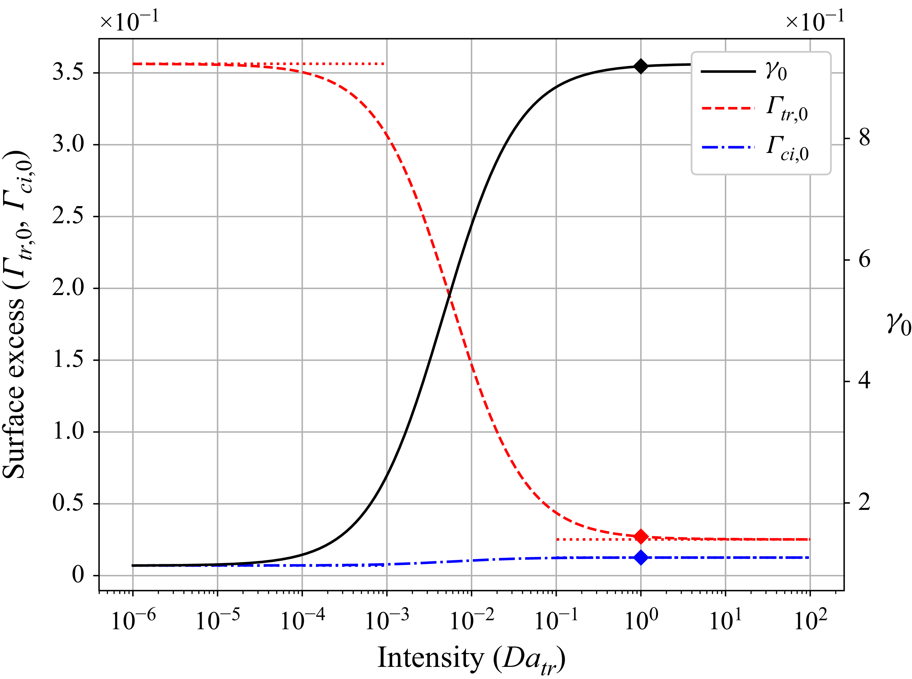


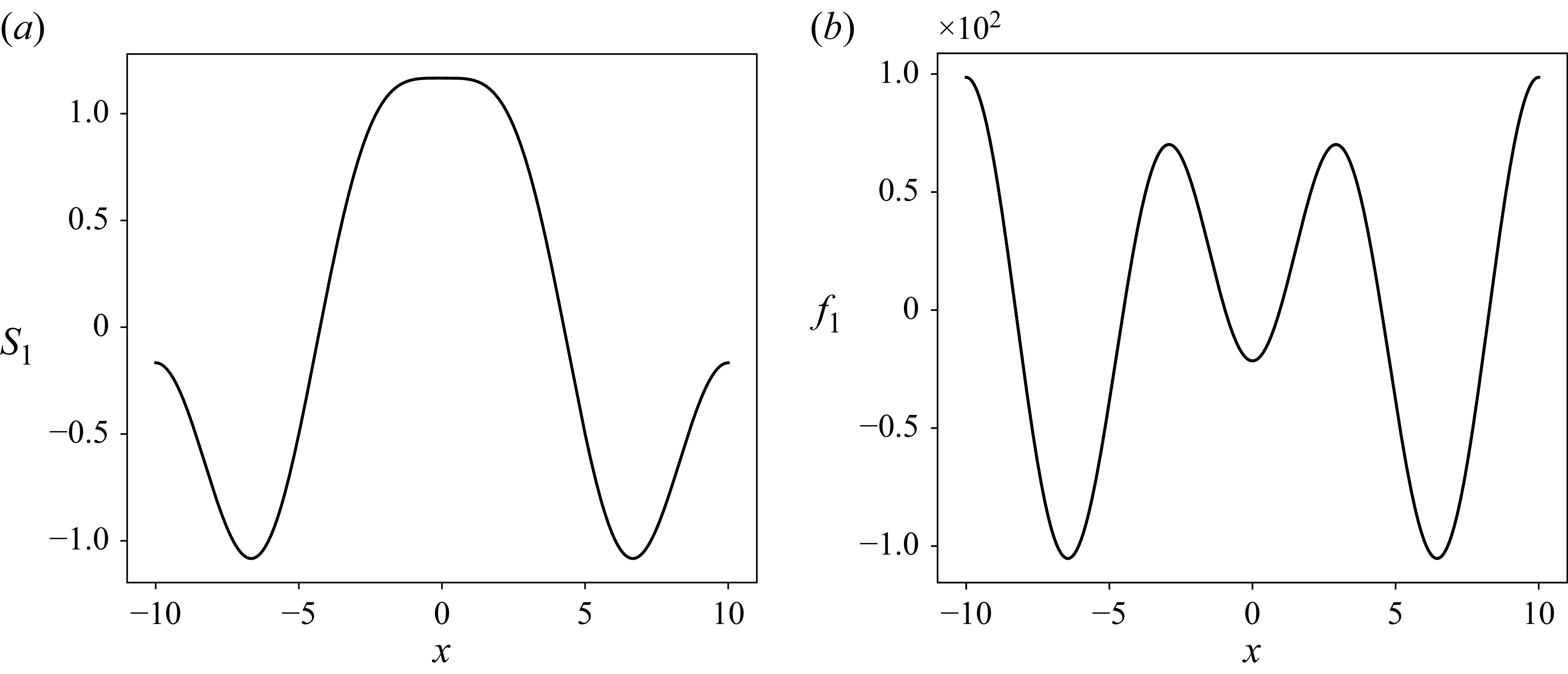


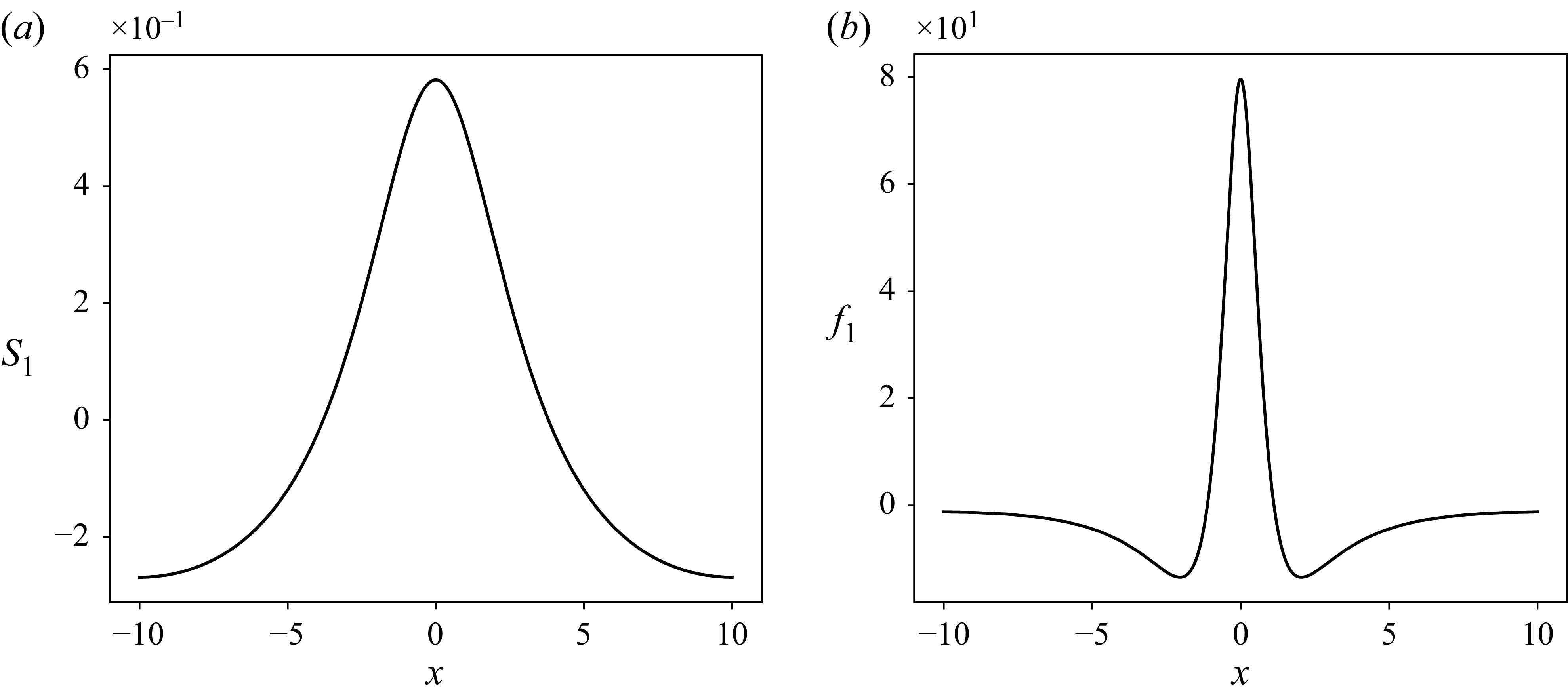


 Open access